Classification and Geometry of General Perceptual Manifolds

SueYeon Chung1,2, Daniel D. Lee2,3, and Haim Sompolinsky2,4,5

1Program in Applied Physics, School of Engineering and Applied Sciences,Harvard University, Cambridge, MA 02138, USA

2Center for Brain Science, Harvard University, Cambridge, MA 02138, USA3School of Engineering and Applied Science, University of Pennysylvania, Philadelphia, PA 19104, USA

4Racah Institute of Physics, Hebrew University, Jerusalem 91904, Israel5Edmond and Lily Safra Center for Brain Sciences, Hebrew University, Jerusalem 91904, Israel

Perceptual manifolds arise when a neural population responds to an ensemble of sensory signalsassociated with different physical features (e.g., orientation, pose, scale, location, and intensity) ofthe same perceptual object. Object recognition and discrimination require classifying the manifoldsin a manner that is insensitive to variability within a manifold. How neuronal systems give riseto invariant object classification and recognition is a fundamental problem in brain theory as wellas in machine learning. Here we study the ability of a readout network to classify objects fromtheir perceptual manifold representations. We develop a statistical mechanical theory for the linearclassification of manifolds with arbitrary geometry revealing a remarkable relation to the mathe-matics of conic decomposition. We show how special anchor points on the manifolds can be usedto define novel geometrical measures of radius and dimension which can explain the classificationcapacity for manifolds of various geometries. The general theory is demonstrated on a number ofrepresentative manifolds, including `2 ellipsoids prototypical of strictly convex manifolds, `1 ballsrepresenting polytopes with finite samples, and ring manifolds exhibiting non-convex continuousstructures that arise from modulating a continuous degree of freedom. The effects of label sparsityon the classification capacity of general manifolds are elucidated, displaying a universal scaling re-lation between label sparsity and the manifold radius. Theoretical predictions are corroborated bynumerical simulations using recently developed algorithms to compute maximum margin solutionsfor manifold dichotomies. Our theory and its extensions provide a powerful and rich frameworkfor applying statistical mechanics of linear classification to data arising from perceptual neuronalresponses as well as to artificial deep networks trained for object recognition tasks.

PACS numbers: 87.18.Sn, 87.19.lv, 42.66.Si, 07.05.Mh

I. INTRODUCTION

A fundamental cognitive task performed by animals andhumans is the invariant perception of objects, requir-ing the nervous system to discriminate between differ-ent objects despite substantial variability in each ob-jects physical features. For example, in vision, themammalian brain is able to recognize objects despitevariations in their orientation, position, pose, lightingand background. Such impressive robustness to physi-cal changes is not limited to vision; other examples in-clude speech processing which requires the detection ofphonemes despite variability in the acoustic signals asso-ciated with individual phonemes; and the discriminationof odors in the presence of variability in odor concen-trations. Sensory systems are organized as hierarchiesconsisting of multiple layers transforming sensory signalsinto a sequence of distinct neural representations. Stud-ies of high level sensory systems, e.g., the inferotempo-ral cortex (IT) in vision [1], auditory cortex in audition[2], and piriform cortex in olfaction [3], reveal that eventhe late sensory stages exhibit significant sensitivity ofneuronal responses to physical variables. This suggeststhat sensory hierarchies generate representations of ob-jects that although not entirely invariant to changes inphysical features, are still readily decoded in an invari-

ant manner by a downstream system. This hypothesis isformalized by the notion of the untangling of perceptualmanifolds [4–6]. This viewpoint underlies a number ofstudies of object recognition in deep neural networks forartificial intelligence [7–10].

To conceptualize perceptual manifolds, consider a set ofN neurons responding to a specific sensory signal asso-ciated with an object as shown in Fig. 1. The neuralpopulation response to that stimulus is a vector in RN .Changes in the physical parameters of the input stimu-lus that do not change the object identity modulate theneural state vector. The set of all state vectors corre-sponding to responses to all possible stimuli associatedwith the same object can be viewed as a manifold in theneural state space. In this geometrical perspective, ob-ject recognition is equivalent to the task of discriminatingmanifolds of different objects from each other. Presum-ably, as signals propagate from one processing stage tothe next in the sensory hierarchy, the geometry of themanifolds is reformatted so that they become “untan-gled,” namely they are more easily separated by a bi-ologically plausible decoder [1]. In this paper, we modelthe decoder as a simple single layer network (the per-ceptron) and ask how the geometrical properties of theperceptual manifolds influence their ability to be sepa-rated by a linear classifier.

arX

iv:1

710.

0648

7v2

[co

nd-m

at.d

is-n

n] 2

6 Fe

b 20

18

2

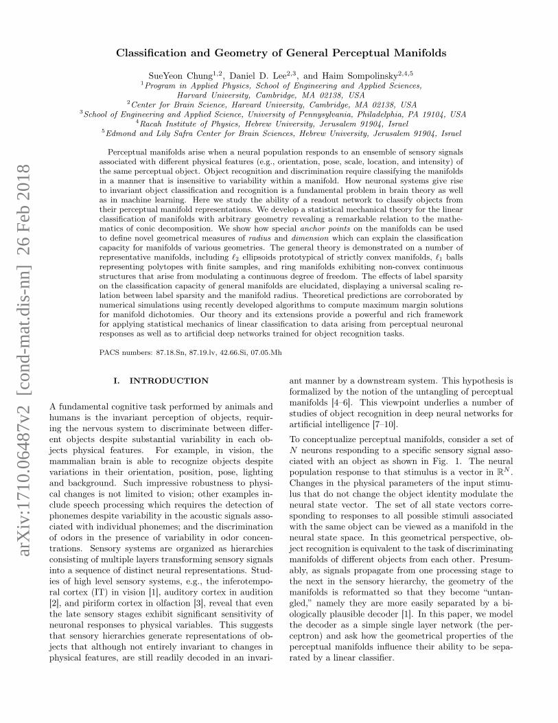
Figure 1. Perceptual manifolds in neural state space. (a)Firing rates of neurons responding to images of a dog shownat various orientations θ and scales s. The response to aparticular orientation and scale can be characterized by anN -dimensional population response. (b) The population re-sponses to the images of the dog form a continuous manifoldrepresenting the complete set of invariances in the RN neu-ral activity space. Other object images, such as those corre-sponding to a cat in various poses, are represented by othermanifolds in this vector space.

Linear separability has previously been studied in thecontext of the classification of points by a perceptron, us-ing combinatorics [11] and statistical mechanics [12, 13].Gardner’s statistical mechanics theory is extremely im-portant as it provides accurate estimates of the percep-tron capacity beyond function counting by incorporatingrobustness measures. The robustness of a linear classifieris quantified by the margin, which measures the distancebetween the separating hyperplane and the closest point.Maximizing the margin of a classifier is a critical objec-tive in machine learning, providing Support Vector Ma-chines (SVM) with their good generalization performanceguarantees [14].

The above theories focus on separating a finite set ofpoints with no underlying geometrical structure and arenot applicable to the problem of manifold classificationwhich deals with separating infinite number of points geo-metrically organized as manifolds. This paper addressesthe important question of how to quantify the capac-ity of the perceptron for dichotomies of input patternsdescribed by manifolds. In an earlier paper, we havepresented the analysis for classification of manifolds ofextremely simple geometry, namely balls [15]. However,the previous results have limited applicability as the neu-ral manifolds arising from realistic physical variations ofobjects can exhibit much more complicated geometries.Can statistical mechanics deal with the classification ofmanifolds with complex geometry, and what specific ge-ometric properties determine the separability of mani-folds?

In this paper, we develop a theory of the linear separa-

bility of general, finite dimensional manifolds. The sum-mary of our key results is as follows:

• We begin by introducing a mathematical modelof general manifolds for binary classification (Sec.II). This formalism allows us to generate genericbounds on the manifold separability capacity fromthe limits of small manifold sizes (classification ofisolated points) as that of large sizes (classificationof entire affine subspaces). These bounds highlightthe fact that for large ambient dimension N , themaximal number P of separable finite-dimensionalmanifolds is proportional to N , even though eachconsists of infinite number of points, setting thestage for a statistical mechanical evaluation of themaximal α = P

N .

• Using replica theory, we derive mean field equa-tions for the capacity of linear separation of finitedimensional manifolds (Sec. III) and for the sta-tistical properties of the optimal separating weightvector. The mean-field solution is given in the formof self consistent Karush-Kuhn-Tucker (KKT) con-ditions involving the manifold anchor point. Theanchor point is a representative support vector forthe manifold. The position of the anchor point ona manifold changes as the orientations of the othermanifolds are varied, and the ensuing statistics ofthe distribution of anchor points play a key role inour theory. The optimal separating plane intersectsa fraction of the manifolds (the supporting mani-folds). Our theory categorizes the dimension of thespan of the intersecting sets (e.g., points, edges,faces, or full manifolds) in relation to the positionof the anchor points in the manifolds’ convex hulls.

• The mean field theory motivates a new definitionof manifold geometry, which is based on the mea-sure induced by the statistics of the anchor points.In particular, we define the manifold anchor radiusand dimension, RM and DM, respectively. Thesequantities are relevant since the capacity of generalmanifolds can be well approximated by the capacityof `2 balls with radii RM and dimensions DM . In-terestingly, we show that in the limit of small man-ifolds, the anchor point statistics are dominatedby points on the boundary of the manifolds whichhave minimal overlap with Gaussian random vec-tors. The resultant Gaussian radius, Rg and dimen-sion, Dg, are related to the well-known Gaussianmean-width of convex bodies (Sec. IV). Beyondunderstanding fundamental limits for classificationcapacity, these geometric measures offer new quan-titative tools for assessing how perceptual mani-folds are reformatted in brain and artificial systems.

• We apply the general theory to three examples,representing distinct prototypical manifold classes.

3

One class consists of manifolds with strictly smoothconvex hulls, which do not contain facets and areexemplified by `2 ellipsoids. Another class is thatof convex polytopes, which arise when the mani-folds consists of a finite number of data points, andare exemplified by `1 ellipsoids. Finally, ring man-ifolds represent an intermediate class: smooth butnonconvex manifolds. Ring manifolds are continu-ous nonlinear functions of a single intrinsic variable,such as object orientation angle. The differencesbetween these manifold types show up most clearlyin the distinct patterns of the support dimensions.However, as we show, they share common trends.As the size of the manifold increases, the capac-ity and geometrical measures vary smoothly, ex-hibiting a smooth cross-over from small radius anddimension with high capacity to large radius anddimension with low capacity. This crossover oc-curs as Rg ∝ 1√

Dg. Importantly, for many realistic

cases, when the size is smaller than the crossovervalue, the manifold dimensionality is substantiallysmaller than that computed from naive second or-der statistics, highlighting the saliency and signifi-cance of our measures for the anchor geometry.

• Finally, we treat the important case of the classi-fication of manifolds with imbalanced (sparse) la-bels, which commonly arise in problems of objectrecognition. It is well known that in highly sparselabels, the classification capacity of random pointsincreases dramatically as (f |log f |)−1, where f � 1is the fraction of the minority labels. Our analysisof sparsely labeled manifolds highlights the inter-play between manifold size and sparsity. In par-ticular, it shows that sparsity enhances the capac-ity only when fR2

g � 1, where Rg is the (Gaus-sian) manifold radius. Notably, for a large regimeof parameters, sparsely labeled manifolds can ap-proximately be described by a universal capacityfunction equivalent to sparsely labeled `2 balls withradii Rg and dimensions Dg, as demonstrated byour numerical evaluations (Sec. VI). Conversely,when fR2

g � 1 , the capacity is low and close to1D where D is the dimensionality of the manifoldaffine subspace, even for extremely small f .

• Our theory provides for the first time, quantita-tive and qualitative predictions for the perceptronclassification of realistic data structures. However,application to real data may require further exten-sions of the theory and are discussed in Section VII.Together, the theory makes an important contri-bution to the development of statistical mechanicaltheories of neural information processing in realis-tic conditions.

Figure 2. Model of manifolds in affine subspaces. D = 2manifold embedded in RN . c is the orthogonal translationvector for the affine space and x0 is the center of the manifold.As the scale r is varied, the manifold shrinks to the point x0,or expands to fill the entire affine space.

II. MODEL OF MANIFOLDS

Manifolds in affine subspaces: We model a set ofP perceptual manifolds corresponding to P perceptualobject. Each manifold Mµ for µ = 1, . . . , P consists of acompact subset of an affine subspace of RN with affinedimension D with D < N . A point on the manifoldxµ ∈Mµ can be parameterized as:

xµ(~S) =

D+1∑i=1

Siuµi , (1)

where the uµi are a set of orthonormal bases of the (D+1)-dimensional linear subspace containing Mµ. The D + 1components Si represents the coordinates of the manifoldpoint within this subspace and are constrained to be inthe set ~S ∈ S. The bold notation for xµ and uµi indicatesthey are vectors in RN whereas the arrow notation for ~Sindicates it is a vector in RD+1. The set S defines theshape of the manifolds and encapsulates the affine con-straint. For simplicity, we will first assume the manifoldshave the same geometry so that the coordinate set S isthe same for all the manifolds; extensions that considerheterogeneous geometries are provided in Sec. VIA.We study the separability of P manifolds into two classes,denoted by binary labels yµ = ±1, by a linear hyperplanepassing through the origin. A hyperplane is described bya weight vector w ∈ RN , normalized so ‖w‖2 = N andthe hyperplane correctly separates the manifolds with amargin κ ≥ 0 if it satisfies,

yµw · xµ ≥ κ (2)

4

for all µ and xµ ∈ Mµ. Since linear separability isa convex problem, separating the manifolds is equiv-alent to separating the convex hulls, conv (Mµ) ={xµ(~S) | ~S ∈ conv(S)

}, where

conv (S) =

{D+1∑i=1

αi~Si | ~Si ∈ S, αi ≥ 0,

D+1∑i=1

αi = 1

}.

(3)The position of an affine subspace relative to the origincan be defined via the translation vector that is closestto the origin. This orthogonal translation vector cµ isperpendicular to all the affine displacement vectors inMµ, so that all the points in the affine subspace haveequal projections on cµ, i.e., ~xµ · cµ = ‖cµ‖ for all xµ ∈Mµ (Fig. 2). We will further assume for simplicity thatthe P norms‖cµ‖ are all the same and normalized to 1.To investigate the separability properties of manifolds, itis helpful to consider scaling a manifoldMµ by an overallscale factor r without changing its shape. We define thescaling relative to a center ~S0 ∈ S by a scalar r > 0, by

rMµ =

{D+1∑i=1

[S0i + r

(Si − S0

i

)]uµi | ~S ∈ S

}(4)

When r → 0, the manifold rMµ converges to a point:xµ0 =

∑i S

0i u

µi . On the other hand, when r → ∞, the

manifold rMµ spans the entire affine subspace. If themanifold is symmetric (such as for an ellipsoid), thereis a natural choice for a center. We will later providean appropriate definition for the center point for general,asymmetric manifolds. In general, the translation vector~c and center ~S0 need not coincide as shown in Fig. 2.However, we will also discuss later the special case ofcentered manifolds in which the translation vector andcenter do coincide.Bounds on linear separability of manifolds: Fordichotomies of P input points in RN at zero margin, κ =0, the number of dichotomies that can be separated by alinear hyperplane through the origin is given by [11]:

C0(P,N) = 2

N−1∑k=0

CP−1k ≤ 2P (5)

where Cnk = n!k!(n−k)! is the binomial coefficient for n ≥

k, and zero otherwise. This result holds for P inputvectors that obey the mild condition that the vectorsare in general position, namely that all subsets of inputvectors of size p ≤ N are linearly independent.For large P and N , the probability 1

2PC0(P,N) of a di-

chotomy being linearly separable depends only upon theratio P

N and exhibits a sharp transition at the criticalvalue of α0 = 2. We are not aware of a comprehen-sive extension of Cover’s counting theorem for generalmanifolds; nevertheless, we can provide lower and upper

bounds on the number of linearly realizable dichotomiesby considering the limit of r → 0 and r → ∞ under thefollowing general conditions.

First, in the limit of r → 0, the linear separability of Pmanifolds becomes equivalent to the separability of the Pcenters. This leads to the requirement that the centers ofthe manifolds, xµ0 , are in general position in RN . Second,we consider the conditions under which the manifolds arelinearly separable when r → ∞ so that the manifoldsspan complete affine subspaces. For a weight vector wto consistently assign the same label to all points on anaffine subspace, it must be orthogonal to all the displace-ment vectors in the affine subspace. Hence, to realize adichotomy of P manifolds when r →∞, the weight vec-torw must lie in a null space of dimensionN−Dtot whereDtot is the rank of the union of affine displacement vec-tors. When the basis vectors uµi are in general position,then Dtot = min (DP,N). Then for the affine subspacesto be separable, PD < N is required and the projec-tions of the P orthogonal translation vectors need alsobe separable in the N−Dtot dimensional null space. Un-der these general conditions, the number of dichotomiesfor D-dimensional affine subspaces that can be linearlyseparated, CD(P,N), can be related to the number ofdichotomies for a finite set of points via:

CD(P,N) = C0(P,N − PD). (6)

From this relationship, we conclude that the ability tolinearly separate D-dimensional affine subspaces exhibitsa transition from always being separable to never beingseparable at the critical ratio P

N = 21+2D for large P and

N (see Supplementary Materials, SM, Sec. S1).

For general D-dimensional manifolds with finite size, thenumber of dichotomies that are linearly separable willbe lower bounded by CD(P,N) and upper bounded byC0(P,N). We introduce the notation, αM(κ), to denotethe maximal load P

N such that randomly labeled mani-folds are linearly separable with a margin κ, with highprobability. Therefore, from the above considerations, itfollows that the critical load at zero margin, αM(κ = 0),is bounded by,

1

2≤ α−1

M (κ = 0) ≤ 1

2+D. (7)

These bounds highlight the fact that in the large N limit,the maximal number of separable finite-dimensional man-ifolds is proportional to N , even though each consists ofan infinite number of points. This sets the stage of astatistical mechanical evaluation of the maximal α = P

N, where P is the number of manifolds, and is describedin the following Section.

5

III. STATISTICAL MECHANICAL THEORY

In order to make theoretical progress beyond the boundsabove, we need to make additional statistical assump-tions about the manifold spaces and labels. Specifically,we will assume that the individual components of uµi aredrawn independently and from identical Gaussian distri-butions with zero mean and variance 1

N , and that thebinary labels yµ = ±1 are randomly assigned to eachmanifold with equal probabilities. We will study the ther-modynamic limit where N,P →∞, but with a finite loadα = P

N . In addition, the manifold geometries as speci-fied by the set S in RD+1, and in particular their affinedimension, D, is held fixed in the thermodynamic limit.Under these assumptions, the bounds in Eq. (7) can beextended to the linear separability of general manifoldswith finite margin κ, and characterized by the reciprocalof the critical load ratio α−1

M (κ),

α−10 (κ) ≤ α−1

M (κ) ≤ α−10 (κ) +D (8)

where α0(κ) is the maximum load for separation of ran-dom i.i.d. points with a margin κ given by the Gardnertheory [12],

α−10 (κ) =

∫ κ

−∞Dt (t− κ)2 (9)

with Gaussian measure Dt = 1√2πe−

t2

2 . For many inter-esting cases, the affine dimension D is large and the gapin Eq. (8) is overly loose. Hence, it is important to de-rive an estimate of the capacity for manifolds with finitesizes and evaluate the dependence of the capacity andthe nature of the solution on the geometrical propertiesof the manifolds as shown below.

A. Mean field theory of manifold separationcapacity

Following Gardner’s framework [12, 13], we compute thestatistical average of logZ, where Z is the volume of thespace of the solutions, which in our case can be writtenas:

Z =

∫dNwδ

(‖w‖2 −N

)Πµ,xµ∈MµΘ (yµw · xµ − κ) ,

(10)Θ (·) is the Heaviside function to enforce the margin con-straints in Eq. (2), along with the delta function to en-sure ‖w‖2 = N . In the following, we focus on the proper-ties of the maximummargin solution, namely the solutionfor the largest load αM for a fixed margin κ, or equiva-lently, the solution when the margin κ is maximized fora given αM.

As shown in Appendix A, we prove that the general formof the inverse capacity, exact in the thermodynamic limit,is:

α−1M (κ) = 〈F (~T )〉~T (11)

where F (~T ) = min~V

{∥∥∥~V − ~T∥∥∥2

| ~V · ~S − κ ≥ 0, ∀~S ∈ S}

and 〈. . .〉~T is an average over random D+ 1 dimensionalvectors ~T whose components are i.i.d. normally dis-tributed Ti ∼ N (0, 1). The components of the vector~V represent the signed fields induced by the solutionvector w on the D+1 basis vectors of the manifold. TheGaussian vector ~T represents the part of the variabilityin ~V due to quenched variability in the manifolds basisvectors and the labels, as will be explained in detailbelow.The inequality constraints in F can be written equiv-alently, as a constraint on the point on the mani-fold with minimal projection on ~V . We thereforeconsider the concave support function of S, gS(~V ) =

min~S

{~V · ~S | ~S ∈ S

}, which can be used to write the

constraint for F (~T ) as

F (~T ) = min~V

{∥∥∥~V − ~T∥∥∥2

| gS(~V )− κ ≥ 0

}(12)

Note that this definition of gS(~V ) is easily mapped tothe conventional convex support function defined via themax operation[16].Karush-Kuhn-Tucker (KKT) conditions: To gaininsight into the nature of the maximum margin solution,it is useful to consider the KKT conditions of the convexoptimization in Eq. 12 [16]. For each ~T , the KKT condi-tions that characterize the unique solution of ~V for F (~T )is given by:

~V = ~T + λS(~T ) (13)

where

λ ≥ 0 (14)

gS(~V )− κ ≥ 0

λ[gS(~V )− κ

]= 0

The vector S(~T ) is a subgradient of the support functionat ~V , S(~T ) ∈ ∂gS

(~V)[16], i.e., it is a point on the convex

hull of S with minimal overlap with ~V . When the sup-port function is differentiable, the subgradient ∂gS

(~V)

is unique and is equivalent to the gradient of the supportfunction,

S(~T ) = ∇gS(~V ) = arg min~S∈S

~V · ~S (15)

6

Since the support function is positively homogeneous,gS(γ~V ) = γgS(~V ) for all γ > 0; thus, ∇gS(~V ) dependsonly on the unit vector V . For values of ~V such thatgS(~V ) is not differentiable, the subgradient is not unique,but S(~T ) is defined uniquely as the particular subgradi-ent that obeys the KKT conditions, Eq. 13-14. In thelatter case, S(~T ) ∈ conv (S) may not reside in S itself.From Eq. (13), we see that the capacity can be writtenin terms of S(~T ) as,

F (~T ) =∥∥∥λS(~T )

∥∥∥2

. (16)

The scale factor λ is either zero or positive, correspondingto whether gS(~V )− κ is positive or zero. If gS(~V )− κ ispositive , then λ = 0 meaning that ~V = ~T and ~T · S(~T )−κ > 0. If ~T · S(~T ) − κ < 0 , then, λ > 0 and ~V 6= ~T . In

this case, multiplying 13 with S(~T ) yields λ∥∥∥S(~T )

∥∥∥2

=

~T · S(~T )− κ. Thus, λ obeys the self consistent equation,

λ =

[~T · S(~T )− κ

]+∥∥∥S(~T )

∥∥∥2 (17)

where the function [x]+ = max(x, 0).

B. Mean field interpretation of the KKT relations

The KKT relations have a nice interpretation within theframework of the mean field theory. The maximum mar-gin solution vector can always be written as a linear com-bination of a set of support vectors. Although there areinfinite numbers of input points in each manifold, the so-lution vector can be decomposed into P vectors, one permanifold,

w =

P∑µ=1

λµyµxµ, λµ ≥ 0 (18)

where xµ ∈ conv (Mµ) is a vector in the convex hull ofthe µ-th manifold. In the large N limit, these vectorsare uncorrelated with each other. Hence, squaring thisequation yields,

‖w‖2 = N =

P∑µ=1

λ2µ

∥∥∥Sµ∥∥∥2

(19)

where Sµ are the coordinates of xµ in the µ-th affinesubspace of the µ-th manifold, see Eq. (1). From this

equation, it follows that α−1 = NP =

⟨λ2∥∥∥S∥∥∥2

⟩which

yields the KKT expression for the capacity, see Eqs. 11and 16.The KKT relations above, are self-consistent equationsfor the statistics of λµand Sµ. The mean field theory de-rives the appropriate statistics from self-consistent equa-tions of the fields on a single manifold. To see this,consider projecting the solution vector w onto the affinesubspace of one of the manifolds, say µ = 1 . We de-fine a D + 1 dimensional vector, ~V 1, as V 1

i = y1w · u1i ,

i = 1, ..., D+1, which are the signed fields of the solutionon the affine basis vectors of the µ = 1 manifold. Then,Eq. (18) reduces to ~V 1 = λ1S

1 + ~T where ~T representsthe contribution from all the other manifolds and sincetheir subspaces are randomly oriented, this contributionis well described as a random Gaussian vector. Finally,self consistency requires that for fixed ~T , S1 is such thatit has a minimal overlap with ~V 1 and represents a pointresiding on the margin hyperplane, otherwise it will notcontribute to the max margin solution. Thus Eq. 13is just the decomposition of the field induced on a spe-cific manifold decomposed into the contribution inducedby that specific manifold along with the contributionscoming from all the other manifolds. The self consis-tent equations 14 as well as 17 relating λ to the Gaussianstatistics of ~T then naturally follow from the requirementthat S1 represents a support vector.

C. Anchor points and manifold supports

The vectors xµ contributing to the solution, Eq. (18),play a key role in the theory. We will denote them orequivalently their affine subspace components, Sµ, as themanifold anchor points. For a particular configuration ofmanifolds, the manifolds could be replaced by an equiv-alent set of P anchor points to yield the same maximummargin solution. It is important to stress, however, thatan individual anchor point is determined not only by theconfiguration of its associated manifold but also by therandom orientations of all the other manifolds. For afixed manifold, the location of its anchor point will varywith the relative configurations of the other manifolds.This variation is captured in mean field theory by thedependence of the anchor point S on the random Gaus-sian vector ~T .In particular, the position of the anchor point in the con-vex hull of its manifold reflects the nature of the relationbetween that manifold and the margin planes. In general,a fraction of the manifolds will intersect with the marginhyperplanes, i.e., they have non-zero λ; these manifoldsare the support manifolds of the system. The nature ofthis support varies and can be characterized by the di-mension, k, of the span of the intersecting set of conv (S)

7

S

�S

S

cone(S)

S�=0

= 0 > 0

S

�S

S

cone(S)

S�>0

(a) (b)

�~c

�~V�~V

�~T �~T

Figure 3. Conic decomposition of −~T = −~V + λS at (a) zeromargin κ = 0 and (b) non-zero margin κ > 0. Given a randomGaussian ~T , ~V is found such that

∥∥∥~V − ~T∥∥∥ is minimized while

−~V being on the polar cone S◦κ. λS is in cone(S) and S isthe anchor point, a projection on the convex hull of S.

with the margin planes. Some support manifolds, whichwe call touching manifolds, intersect with the margin hy-perplane only with their anchor point. They have a sup-port dimension k = 1, and their anchor point S is on theboundary of S. The other extreme is fully supportingmanifolds which completely reside in the margin hyper-plane. They are characterized by k = D+1. In this case,~V is parallel to the translation vector ~c of S. Hence, allthe points in S are support vectors, and all have thesame overlap, κ, with ~V . The anchor point, in this case,is the unique point in the interior of conv(S) which obeysthe self consistent equation, 13, namely that it balancesthe contribution from the other manifolds to zero outthe components of ~V that are orthogonal to ~c. In thecase of smooth convex hulls (i.e., when S is strongly con-vex), no other manifold support configurations exist. Forother types of manifolds, there are also partially support-ing manifolds, whose convex hull intersection with themargin hyperplanes consist of k dimensional faces with1 < k < D+ 1. The associated anchor points then resideinside the intersecting face. For instance, k = 2 impliesthat S lies on an edge whereas k = 3 implies that S lieson a planar 2-face of the convex hull. Determining thedimension of the support structure that arises for various~T is explained below.

D. Conic decomposition

The KKT conditions can also be interpreted in terms ofthe conic decomposition of ~T , which generalizes the no-tion of the decomposition of vectors onto linear subspacesand their null spaces via Euclidean projection. The con-vex cone of the manifold S is defined as cone (S) =

{∑D+1i=1 αi~Si | ~Si ∈ S, αi ≥ 0

}, see Fig. 3. The shifted

polar cone of S, denoted S◦κ, is defined as the convex setof points given by,

S◦κ ={~U ∈ RD+1 | ~U · ~S + κ ≤ 0, ∀~S ∈ S

}(20)

and is illustrated for κ = 0 and κ > 0 in Fig. 3. Forκ = 0, Eq. (20) is simply the conventional polar coneof S [17]. Equation (13) can then be interpreted asthe decomposition of −~T into the sum of two compo-nent vectors: one component is −~V , i.e., its Euclideanprojection onto S◦κ; the other component λS(~T ) is lo-cated in cone (S). When κ = 0, the Moreau decom-position theorem states that the two components areperpendicular: ~V ·

(λS(~T )

)= 0 [18]. For non-zero κ,

the two components need not be perpendicular but obey~V ·(λS(~T )

)= κλ.

The position of vector ~T in relation to the cones, cone(S)and S◦κ, gives rise to qualitatively different expressionsfor F

(~T)and contributions to the solution weight vec-

tor and inverse capacity. These correspond to the differ-ent support dimensions mentioned above. In particular,when -~T lies inside S◦κ , ~T = ~V and λ = 0 so the sup-port dimension, k = 0. On the other hand, when −~Tlies inside cone (S), ~V = κ~c and the manifold is fullysupporting, k = D + 1.

E. Numerical solution of the mean field equations

The solution of the mean field equations consists of twostages. First, S is computed for a particular ~T and thenthe relevant contributions to the inverse capacity are av-eraged over the Gaussian distribution of ~T . For simplegeometries such as `2 ellipsoids, the first step may besolved analytically. However, for more complicated ge-ometries, both steps need to be performed numerically.The first step involves determining ~V and S for a given ~Tby solving the quadratic semi-infinite programming prob-lem (QSIP), Eq. (12), over the manifold S which maycontain infinitely many points. A novel “cutting plane”method has been developed to efficiently solve the QSIPproblem, see SM (Sec. S4). Expectations are computedby sampling Gaussian ~T in D+ 1 dimensions and takingthe appropriate averages, similar to procedures for othermean field methods. The relevant quantities correspond-ing to the capacity are quite concentrated and convergequickly with relatively few samples.In following Sections, we will also show how the meanfield theory compares with computer simulations thatnumerically solve for the maximum margin solution ofrealizations of P manifolds in RN , given by Eq. (2), fora variety of manifold geometries. Finding the maximum

8

margin solution is challenging as standard methods tosolving SVM problems are limited to a finite number ofinput points. We have recently developed an efficientalgorithm for finding the maximum margin solution inmanifold classification and have used this method in thepresent work (see [19] and SM (Sec. S5)).

IV. MANIFOLD GEOMETRY

A. Longitudinal and intrinsic coordinates

In this section, we address how the capacity to sepa-rate a set of manifolds can be related to their geome-try, in particular to their shape within the D-dimensionalaffine subspace. Since the projections of all points in amanifold onto the translation vector, cµ, are the same,~xµ · cµ = ‖cµ‖ = 1, it is convenient to parameterize theD+ 1 affine basis vectors such that uµD+1 = cµ. In thesecoordinates, the D+ 1 dimensional vector representationof cµ is ~C = (0, 0, . . . , 0, 1). This parameterization is con-venient since it constrains the manifold variability to bein the first D components of ~S while the D+1 coordinateis a longitudinal variable measuring the distance of themanifold affine subspace from the origin. We can thenwrite the D + 1 dimensional vectors ~T = (~t, t0) wheret0 = ~T · ~C, ~V = (~v, v0), ~S =(~s, 1), S = (s, 1) , wherelower case vectors denote vectors in RD. We will also re-fer to the D-dimensional intrinsic vector, s, as the anchorpoint. In this notation, the capacity, Eq. (16)-(17) canbe written as,

α−1M (κ) =

∫D~t

∫Dt0

[−t0 − ~t · s(~t, t0) + κ

]2+

1 +∥∥s(~t, t0)

∥∥2 (21)

It is clear from this form that when D = 0, or when allthe vectors in the affine subspace obey s(~t, t0) = 0 , thecapacity reduces to the Gardner result, Eq. (9). Since~V · S=~v · s + v0, for all S , g(~V ) = g(~v) + v0 , and thesupport function can be expressed as,

g(~v) = min~s{~v · ~s | ~s ∈ S} . (22)

The KKT relations can be written as ~v = ~t +λ~s where λ = v0 − t0 ≥ 0, g(~v) ≥ κ − v0,λ [g(~v) + v0 − κ] = 0, and s minimizes the over-lap with ~v. The resultant equation for λ (or v0)

is λ =[−t0 − ~t · s(~t, t0) + κ

]+/(

1 +∥∥s(~t, t0)

∥∥2)

whichagrees with Eq. 17.

B. Types of supports

Using the above coordinates, we can elucidate the condi-tions for the different types of support manifolds defined

in the previous section. To do this, we fix the randomvector ~t and consider the qualitative change in the anchorpoint, s(~t, t0) as t0 decreases from +∞ to −∞.Interior manifolds (k = 0): For sufficiently positive t0,the manifold is interior to the margin plane, i.e., λ = 0with corresponding support dimension k = 0. Althoughnot contributing to the inverse capacity and solution vec-tor, it is useful to associate anchor points to these mani-folds defined as the closest point on the manifold to themargin plane: s(~t) = arg min~s∈S ~t ·~s = ∇g(~t) since ~v = ~t.This definition ensures continuity of the anchor point forall λ ≥ 0.This interior regime holds when g(~t) > κ− t0, or equiva-lently for t0 − κ > ttouch(~t) where

ttouch(~t) = −g(~t) (23)

Non-zero contributions to the capacity only occur outsidethis interior regime when g(~t) + t0−κ < 0, in which caseλ > 0. Thus, for all support dimensions k > 0, thesolution for ~v is active, satisfying the equality condition,g(~v) + v0 − κ = 0, so that from Eq. (13):

g(~v) + t0 − κ− λ = 0, (24)

outside the interior regime.Fully supporting manifolds (k = D + 1): When t0is sufficiently negative, v0 = κ, ~v = 0 and λ = t0 − κ.The anchor point s(~T ) which obeys the KKT equationsresides in the interior of conv (S),

s(~t, t0) =−~t

κ− t0(25)

For a fixed ~t, t0 must be negative enough, t0 − κ < tfs,where

tfs(~t) = arg max

{t0 |

−~tκ− t0

∈ conv(S)

}(26)

guaranteeing that s(~t, t0) ∈ conv (S). The contributionof this regime to the capacity is

F (~T ) =∥∥~v − ~t∥∥2

+ (v0 − t0)2 =∥∥~t∥∥2

+ (κ− t0)2, (27)

see Eq. (12). Finally, for values of t0 such that tfs(~t) ≤t0 − κ ≤ ttouch(~t), the manifolds are partially support-ing with support dimension 1 ≤ k ≤ D. Examples ofdifferent supporting regimes are illustrated in Figure 4.

C. Effects of size and margin

We now discuss the effect of changing manifold size andthe imposed margin on both capacity and geometry. As

9

described by Eq. (4), change in the manifold size corre-sponds to scaling every s by a scalar r.Small size: If r → 0, the manifold shrinks to a point(the center), whose capacity reduces to that of isolatedpoints. However, in the case where D � 1 , the capacitymay be affected by the manifold structure even if r � 1,see section IVF. Nevertheless, the underlying supportstructure is simple. When r is small, the manifolds haveonly two support configurations. For t0 − κ > 0, themanifold is interior with: λ = 0 , v0 = t0 and ~v = ~t.When t0 − κ < 0, the manifold becomes touching withsupport dimension k = 1. In that case, because s has asmall magnitude, ~v ≈ ~t, λ ≈ κ − t0, and v0 ≈ κ. Thus,in both cases, ~v is close to the Gaussian vector ~t. Theprobability of other configurations vanishes.Large size: In the large size limit r → ∞, separat-ing the manifolds is equivalent to separating the affinesubspaces. As we show in Appendix C, when r � 1,there are two main support structures. With probabil-ity H (−κ) =

∫∞−κDt0 the manifolds are fully supporting,

namely the underlying affine subspaces are parallel to themargin plane. This regime contributes to the inverse ca-pacity an amountH (−κ)D+α−1

0 (κ). The other regimes(touching or partially supporting) are such that the an-gle between the affine subspace and the margin plane isalmost zero, and contribute an amount H(κ)D to theinverse capacity. Combining the two contributions, weobtain for large sizes, α−1

M = D+α−10 (κ), consistent with

Eq. (8).

Large margin: For a fixed ~T , Eq. (26) implies thatlarger κ increases the probability of being in the support-ing regimes. Increasing κ also shrinks the magnitude of saccording to Eq. (25). Hence, when κ� 1, the capacitybecomes similar to that of P random points and the cor-responding capacity is given by αM ≈ κ−2, independentof manifold geometry.Manifold centers: The theory of manifold classificationdescribed in Sec. III does not require the notion of amanifold center. However, understanding how scalingthe manifold sizes by a parameter r in (4) affects theircapacity, the center points about which the manifoldsare scaled need to be defined. For many geometries, thecenter is a point of symmetry such as for an ellipsoid.For general manifolds, a natural definition would be thecenter of mass of the anchor points S(~T ) averaging overthe Gaussian measure of ~T . We will adopt here a simplerdefinition for the center provided by the Steiner point forconvex bodies [20], ~S0 = (~s0, 1) with

~s0 =⟨∇gS(~t)

⟩~t

(28)

and the expectation is over the Gaussian measure of~t ∈ RD. This definition coincides with the center of massof the anchor points when the manifold size is small. Fur-thermore, it is natural to define the geometric properties

Interior (k=0) Touching (k=1) Fully supporting (k=3)

(a1)

s ss

(a2) (a3)�~v = �~t �~v �~t �~t

�~v = 0

�~v

Interior (k=0) Touching (k=1) Fully supporting (k=3)Partially supporting (k=2)

(b1)

s s ss

(b2) (b3) (b4)�~v = �~t �~v�~t

�~t�~v �~t

�~v = 0

Figure 4. Determining the anchor points of the Gaussiandistributed vector (~t, t0) onto the convex hull of the mani-fold, denoted as s(~t, t0). Here we show for the same vector~t, the change in s(~t, t0) as t0 decreases from +∞ to −∞.(a) D = 2 strictly convex manifold. For sufficiently nega-tive −t0 the vector −~t obeys the constraint g(~t) − t0 > κ,hence −~t = −~v and the configuration corresponds to an in-terior manifold (support dimension k = 0). For intermediatevalues where (ttouch > t0 − κ > tfs), (−~t,−t0) violates theabove constraints and s is a point on the boundary of themanifold that maximizes the projection on the manifold ofa vector (−~v,−v0) that is the closest to (−~t,−t0) and obeysg(~v) + t0 − λ = κ. Finally, for larger values of −t0, ~v = 0and s is a point in the interior of the manifold in the direc-tion of −~t (fully supporting with k = 3). (b) D = 2 squaremanifold. Here, in both the interior and touching regimes, sis a vertex of the square. In the fully supporting regime, theanchor point is in the interior and collinear to −~t. There isalso a partially supporting regime when −t0 is slightly belowtfs. In this regime, −~v is perpendicular to one of the edgesand s resides on an edge, corresponding to manifolds whoseintersection with the margin planes are edges (k = 2).

of manifolds in terms of centered manifolds where themanifolds are shifted within their affine subspace so thatthe center and orthogonal translation vector coincide, i.e.~s0 = ~c with

∥∥~s0∥∥ = ‖~c‖ = 1. This means that all lengths

are defined relative to the distance of the centers fromthe origin and the D-dimensional intrinsic vectors ~s givethe offset relative to the manifold center.

D. Manifold anchor geometry

The capacity equation (21) motivates defining geomet-rical measures of the manifolds, which we call manifoldanchor geometry. Manifold anchor geometry is based onthe statistics of the anchor points s(~t, t0) induced by theGaussian random vector (~t, t0) which are relevant to thecapacity in Eq. (21). These statistics are sufficient fordetermining the classification properties and supportingstructures associated with the maximummargin solution.We accordingly define the manifold anchor radius and di-mension as:Manifold anchor radius: denoted RM, is defined bythe mean squared length of s(~t, t0),

R2M =

⟨∥∥s(~t, t0)∥∥2⟩~t,t0

(29)

10

Manifold anchor dimension: DM, is given by

DM =⟨(~t · s(~t,t0)

)2⟩~t,t0

(30)

where s is a unit vector in the direction of s. The anchordimension measures the angular spread between ~t andthe corresponding anchor point s in D dimensions. Notethat the manifold dimension obeys DM ≤

⟨∥∥~t∥∥2⟩

= D.Whenever there is no ambiguity, we will call RM and DMthe manifold radius and dimension, respectively.These geometric descriptors offer a rich description ofthe manifold properties relevant for classification. Since~v and s depend in general on t0−κ, the above quantitiesare averaged not only over ~t but also over t0. For thesame reason, the manifold anchor geometry also dependsupon the imposed margin.

E. Gaussian geometry

We have seen that for small manifold sizes, ~v ≈ ~t, and theanchor points s can be approximated by s(~t) = ∇gS(t).Under these conditions, the geometry simplifies as shownin Fig. 5. For each Gaussian vector ~t ∈ RD, s(~t) isthe point on the manifold that first touches a hyper-plane normal to -~t as it is translated from infinity to-wards the manifold. Aside from a set of measure zero,this touching point is a unique point on the boundary ofconv(S). This procedure is similar to that used to definethe well known Gaussian mean-width, which in our nota-tion equals w(S) = −2

⟨gS(~t)

⟩~t[21]. Note that for small

sizes, the touching point does not depend on t0 or κ so itsstatistics are determined only by the shape of conv (S)relative to its center. This motivates defining a simplermanifold Gaussian geometry denoted by the subscript g,which highlights its dependence over a D dimensionalGaussian measure for ~t.Gaussian radius: denoted by Rg, measures the meansquare amplitude of the Gaussian anchor point, sg(~t) =∇gS(t):

R2g =

⟨∥∥sg (~t)∥∥2⟩~t

(31)

where the expectation is over D-dimensional Gaussian ~t.Gaussian dimension: Dg, is defined by,

Dg =⟨(~t · sg

(~t))2⟩

~t(32)

where sg is the unit vector in the direction of sg. WhileR2

g measures the total variance of the manifold, Dg mea-sures the angular spread of the manifold, through thestatistics of the angle between ~t and its Gaussian anchorpoint. Note that Dg ≤

⟨∥∥~t∥∥2⟩

= D.

sg(~t) sg(~t)sg(~t)

�~t �~t �~t(a) (b) (c)

Figure 5. Gaussian anchor points: Mapping from ~t to pointssg(~t), showing the relation between −~t and the point on themanifold that touches a hyperplane orthogonal to ~t . D =2 manifolds shown: (a) circle; (b) `2 ellipsoid; (c) polytopemanifold. In (c), only for values of ~t of measure zero (when~t is exactly perpendicular to an edge), sg(~t) will lie along theedge, otherwise it coincides with a vertex of the polytope. Inall cases, sg(~t) will be in the interior of the convex hulls onlyfor ~t = 0. Otherwise, it is restricted to their boundary.

It is important to note that even in this limit, our ge-ometrical definitions are not equivalent to conventionalgeometrical measures such as the longest chord or sec-ond order statistics induced from a uniform measure overthe boundary of conv (S). For the special case of D-dimensional `2 balls with radius R, sg

(~t)is the point

on the boundary of the ball in the direction of ~t so thatRg = R andDg = D. However, for general manifolds, Dgcan be much smaller than the manifold affine dimensionD as illustrated in some examples later.

We recapitulate the essential difference between theGaussian geometry and the full manifold anchor geome-try. In the Gaussian case, the radius is an intrinsic prop-erty of the shape of the manifold in its affine subspaceand is invariant to changing its distance from the ori-gin. Thus, scaling the manifold by a global scale factorr as defined in Eq. (4) results in scaling Rg by the fac-tor r. Likewise, the dimensionality Dg is invariant to aglobal scaling of the manifold size. In contrast, the an-chor geometry does not obey such invariance for largermanifolds. The reason is that the anchor point dependson the longitudinal degrees of freedom, namely on thesize of the manifold relative to the distance from the cen-ter. Hence, RM need not scale linearly with r, and DMwill also depend on r. Thus, the anchor geometry canbe viewed as describing the general relationship betweenthe signal (center distance) to noise (manifold variability)in classification capacity. We also note that the manifoldanchor geometry automatically accounts for the rich sup-port structure described in Section IVD. In particular,as t0 decreases, the statistics of the anchor points changefrom being concentrated on the boundary of conv(S) toits interior. Additionally for manifolds which are notstrictly convex and intermediate values of t0, the anchorstatistics become concentrated on k-dimensional facetsof the convex hull corresponding to partially supportedmanifolds.

We illustrate the difference between the two geometries

11

GaussianPolar-constrained

0 2.5 50

0.02

0.96

0.98

1(a) (b)

!" #

$% = ', $) = ). ' $% = ', $) = ). '$% = ', $) = ' (c)

!"

2DEllipsoidDistributionofS,theta

0 2.5 50

0.05

0.1

0.15

0.2GaussianPolar-constrained

0 10 20 30 400

0.1

0.2

0.3

0.4GaussianPolar-constrained

Gaussian

Manifold Anchor

Figure 6. Distribution of ‖s‖ (norm of manifold anchor vec-tors) and θ = ∠(−~t, s) for D = 2 ellipsoids. (a) Distributionof s for `2 ball with R = 5. The Gaussian geometry is peakedat ‖s‖ = r (blue), while ‖s‖ < r has non-zero probability forthe manifold anchor geometry (red). (b-c) D = 2 ellipsoids,with radii R1 = 5 and R2 = 1

2R1. (b) Distribution of ‖s‖

for Gaussian geometry (blue) and anchor geometry (red). (c)Corresponding distribution of θ = ∠(−~t, s).

in Fig. 6 with two simple examples: a D = 2 `2 ball anda D = 2 `2 ellipse. In both cases we consider the distri-bution of ‖s‖ and θ = cos−1

(−t · s

), the angle between

−~t and s. For the ball with radius r, the vectors −~t and sare parallel so the angle is always zero. For the manifoldanchor geometry, s may lie inside the ball in the fullysupporting region. Thus the distribution of ‖s‖ consistsof a mixture of a delta function at r corresponding tothe interior and touching regions and a smoothly varyingdistribution corresponding to the fully supporting region.Fig. 6 also shows the corresponding distributions for atwo dimensional ellipsoid with major and minor radius,R1 = r and R2 = 1

2r. For the Gaussian geometry, thedistribution of ‖s‖ has finite support between R1 and R2,whereas the manifold anchor geometry has support alsobelow R2. Since ~t and s need not be parallel, the dis-tribution of the angle varies between zero and π

4 , withthe manifold anchor geometry being more concentratednear zero due to contributions from the fully supportingregime. In Section (VI), we will show how the Gaus-sian geometry becomes relevant even for larger manifoldswhen the labels are highly imbalanced, i.e. sparse classi-fication.

F. Geometry and classification of high dimensionalmanifolds

In general, linear classification as expressed in Eq. (21)depends on high order statistics of the anchor vectorss(~t, t0). Surprisingly, our analysis shows that for high di-mensional manifolds, the classification capacity can bedescribed in terms of the statistics of RM and DM alone.This is particularly relevant as we expect that in manyapplications, the affine dimension of the manifolds islarge. More specifically, we define high-dimensional man-ifolds as manifolds where the manifold dimension is large,i.e., DM � 1 (but still finite in the thermodynamic limit).

In practice we find that DM & 5 is sufficient. Our anal-ysis below elucidates the interplay between size and di-mension, namely, how small RM needs to be for high di-mensional manifolds to have a substantial classificationcapacity.In the high-dimensional regime, the mean field equationssimplify due to self averaging of terms involving sumsof components ti and si. The two quantity, ~t · s, thatappears in the capacity, (21), can be approximated as−~t · s ≈ κM where we introduce the effective manifoldmargin κM = RM

√DM . Combined with ‖s‖2 ≈ R2

M ,we obtain

αM(κ) ≈ α0

(κ+ κM√1 +R2

M

)(33)

where α0 is the capacity for P random points, Eq. (9).To gain insight into this result we note that the effectivemargin on the center is its mean distance from the pointclosest to the margin plane, s, which is roughly the meanof ~t·s ≈ RM

√DM. The denominator in Eq. (33) indicates

that the margin needs to be scaled by the input norm,√1 +R2

M. In Appendix B, we show that Eq. (33) canalso be written as

αM(κ) ≈ αBall (κ, RM, DM) (34)

namely, the classification capacity of a general high di-mensional manifold is well approximated by that of `2balls with dimension DM and radius RM.Scaling regime: Eq. (33) implies that to obtain a fi-nite capacity in the high-dimensional regime, the effectivemargin κM = RM

√DM needs to be of order unity which

requires the radius to be small, scaling for large DM asRM = O

(D− 1

2

M

). In this scaling regime, the calculation

of the capacity and geometric properties are particularlysimple. As argued above, when the radius is small, thecomponents of s are small, hence ~v ≈ ~t, and the Gaus-sian statistics for the geometry suffice. Thus, we canreplace RM and DM in Eqs. (33)- (34) by Rg and Dg,respectively. Note that in the scaling regime, the factorproportional to 1 +R2

g in Eq. (33) is the next order cor-rection to the overall capacity since Rg is small. Notably,the margin in this regime, κg = Rg

√Dg, is equal to half

the Gaussian mean width of convex bodies, κg ≈ 12w(S)

[22]. As for the support structure, since the manifold sizeis small, the only significant contributions arise from theinterior (k = 0) and touching (k = 1) supports.Beyond the scaling regime: When Rg is not small,the anchor geometry, RM and DM, cannot be adequatelydescribed by the Gaussian statistics, Rg and Dg. In thiscase, the manifold margin κM = RM

√DM is large and

Eq. (33) reduces to :

12

αM ≈1 +R−2

MDM

(35)

where we have used α0 (κ) ≈ κ−2 for large margins andassumed that κ � κM. For strictly convex high dimen-sional manifolds with RM = O(1), only the touchingregime (k = 1) contributes significantly to the geome-try and hence to the capacity. For manifolds that arenot strictly convex, partially supporting solutions withk � D can also contribute to the capacity.Finally, when RM is large, fully supporting regimes withk ≈ D contribute to the geometry, in which case, themanifold anchor dimension approaches the affine dimen-sion DM → D and Eqs. (33) and (35)reduce to αM ≈ 1

D ,as expected.

V. EXAMPLES

A. Strictly convex manifolds: `2 ellipsoids

The family of `2 ellipsoids are examples of manifoldswhich are strictly convex. Strictly convex manifold havesmooth boundaries that do not contain corners, edges, orflats (see Appendix B). Thus, the description of the an-chor geometry and support structures is relatively simple.The reason is that the anchor vectors s(~t, t0) correspondto either interior (k = 0), touching (k = 1), or fully sup-porting (k = D+1), while partial support (1 < k < D+1)is not possible. The `2 ellipsoid geometry can be solvedanalytically; nevertheless, because it has less symmetrythan the sphere, it exhibits some salient properties ofmanifold geometry such as nontrivial dimensionality andnon-uniform measure of the anchor points.We assume the ellipsoids are centered relative to theirsymmetry centers as described in Sec. IV, and can beparameterized by the set of points: Mµ = xµ0 +

∑Di=1 siu

µi

where

S =

{~s |

D∑i=1

(siRi

)2

≤ 1

}. (36)

The components of uµi and of the ellipsoid centers x0µ

are i.i.d. Gaussian distributed with zero mean and vari-ance 1√

Nso that they are orthonormal in the large N

limit. The radii Ri represent the principal radii of the el-lipsoids relative to the center. The anchor points s(~t, t0)can be computed explicitly (details in the Appendix B),corresponding to three regimes.Interior (k = 0), occurs when t0 − κ ≥ ttouch(~t) where,

ttouch(~t) =

√√√√ D∑i=1

R2i t

2i (37)

Here λ = 0, resulting in zero contribution to the inversecapacity.The touching regime (k = 1) holds when ttouch(~t) > t0 −κ > tfs(~t) and

tfs(~t) = −

√√√√ D∑i=1

(tiRi

)2

(38)

Finally, the fully supporting regime (k = D + 1) occurswhen tfs(~t) > t0−κ. The full expression for the capacityfor `2 ellipsoids is given in Appendix, Section B. Below,we focus on the interesting cases of ellipsoids withD � 1.High-dimensional ellipsoids: It is instructive to ap-ply the general analysis of high dimensional manifolds toellipsoids with D � 1. We will distinguish between dif-ferent size regimes by assuming that all the radii of theellipsoid are scaled by a global factor r. In the high di-mensional regime, due to self-averaging, the boundariesof the touching and fully supporting transitions can beapproximated by,

ttouch =

√√√√ D∑i=1

R2i (39)

tfs = −

√√√√ D∑i=1

R−2i (40)

both independent of ~t. Then as long as Ri√D are not

large (see below), tfs → −∞, and the probability of fullysupporting vanishes. Discounting the fully supportingregime, the anchor vectors s(~t, t0) are given by,

si = −λiti (41)

λi =R2i

Z(1 +R2i )

(42)

where the normalization factor Z2 =∑Di=1

R2i

(1+R2i )

2 (seeAppendix B) . The capacity for high-dimensional ellip-soids, is determined via Eq. (33) with manifold anchorradius,

R2M =

D∑i=1

λ2i (43)

and anchor dimension,

DM =

(∑Di=1 λi

)2

∑Di=1 λ

2i

(44)

13

Note that RM/r and DM are not invariant to scaling theellipsoid by a global factor r, reflecting the role of thefixed centers.The anchor covariance matrix: We can also computethe covariance matrix of the anchor points. This matrixis diagonal in the principal directions of the ellipsoid, andits eigenvalues are λ2

i . It is interesting to compare DMwith a well known measure of an effective dimension of acovariance matrix, the participation ratio [23, 24]. Givena spectrum of eigenvalues of the covariance matrix, in ournotation λ2

i , we can define a generalized participation

ratio as PRq =(∑Di=1 λ

qi )

2∑Di=1 λ

2qi

, q > 0. The conventionalparticipation ratio uses q = 2, whereas DM uses q = 1 .Scaling regime: In the scaling regime where the radiiare small, the radius and dimension are equivalent to theGaussian geometry:

R2g =

∑Di=1R

4i∑D

i=1R2i

(45)

Dg =

(∑Di=1R

2i

)2

∑Di=1R

4i

(46)

and the effective margin is given as,

κg =

(D∑i=1

R2i

)1/2

(47)

As can be seen, Dg and Rgr are invariant to scaling all the

radii by r, as expected. It is interesting to compare theabove Gaussian geometric parameters with the statisticsinduced by a uniform measure on the surface of the ellip-soid. In this case, the covariance matrix has eigenvaluesλ2i = R2

i and the total variance is equal to∑iR

2i . In

contrast, in the Gaussian geometry, the eigenvalues ofthe covariance matrix, λ2

i , are proportional to R4i . This

and the corresponding expression (45) for the squaredradius is the result of a non-uniform induced measure onthe surface of the ellipse in the anchor geometry, even inits Gaussian limit.Beyond the scaling regime: When Ri = O(1), thehigh dimensional ellipsoids all become touching manifoldssince ttouch → −∞ and tfs → ∞. The capacity is smallbecause κM � 1, and is given by Eq. (35) with Eqs.(43)-(44). Finally, when all Ri � 1, we have,

R2M =

D∑Di=1R

−2i

=1

〈R−2i 〉i

(48)

Here RM scales with the global scaling factor, r, DM = D,and α−1 = D. Although the manifolds are touching,their angle relative to the margin plane is near zero.

10-2 10-1 100 101 102

R0

0

0.5

1

1.5

2EllipsoidsNumerics (Bimodal)

(a) (b)

(c) (d)

0

0.2

0.4

0.6

0 1 D+1

R0=1.00e-02

0

0.5

1

0 1 D+1

R0=1.00e+02

0

0.5

1

0 1 D+1

R0=1.00e+00(e1) (e2) (e3)

r=0.01 r=1 r=100

R0

10-2 100 102

RM/R0

0

0.2

0.4

0.6

0.8

1

r

R "/$

10-2 10-1 100 101 102

r

0

50

100

150

200

D M

r

% = 200

50 100 150 2000

0.2

0.4

0.6

0.8

1

Dimension

R )

r = 1

r

%*

Figure 7. Bimodal `2 ellipsoids. (a) Ellipsoidal radii Ri withr = 1 (b) Classification capacity as a function of scaling factorr: (blue lines) full mean field theory capacity, (black dashed)approximation of the capacity given by equivalent ball withRM and DM, (circles) simulation capacity, averaged over 5repetitions, measured with 50 dichotomies per each repeti-tion. (c) Manifold dimension DM as a function of r. (d)Manifold radius RM relative to r. (e) Fraction of manifoldswith support dimension k for different values of r: k = 0 (in-terior), k = 1 (touching), k = D + 1 (fully supporting). (e1)Small r = 0.01, where most manifolds are interior or touching(e2) r = 1, where most manifolds are in the touching regime(e3) r = 100, where the fraction of fully supporting manifolds

is 0.085, predicted by H(−tfs) = H(√∑

iR−2i ) (Eq. 40).

When Ri ≈√D or larger, the fully supporting transi-

tion tfs becomes order one and the probability of fullysupporting is significant.

In Fig. 7 we illustrate the behavior of highD-dimensionalellipsoids, using ellipsoids with a bimodal distribution oftheir principal radii, Ri: Ri = r, for 1 ≤ i ≤ 10 andRi = 0.1r, for 11 ≤ i ≤ 200 (Fig. 7(a)). Their proper-ties are shown as a function of the overall scale r. Fig.7(b) shows numerical simulations of the capacity, the fullmean field solution as well as the spherical high dimen-sional approximation (with RM and DM). These calcu-lations are all in good agreement, showing the accuracyof the mean field theory and spherical approximation.As seen in (b)-(d), the system is in the scaling regimefor r < 0.3. In this regime, the manifold dimension isconstant and equals Dg ≈ 14, as predicted by the par-

14

10-3 10-2 10-1 100 101 102

r

024681012

RM/r

10-3 10-2 10-1 100 101 102r

10-2

10-1

100

toR_MorR_Ewhatever]

(a) (b)

Dimension200 400 600 800 1000

Ri

10-1

100

101

(c) (d)

10-2 100 102

r

0

250

500

750

1000

DM

! = 1023

r = 1

!'

Figure 8. Ellipsoids with radii computed from realistic imagedata. (a) SVD spectrum, Ri, taken from the readout layer ofGoogLeNet from a class of ImageNet images with N = 1024and D = 1023. The radii are scaled by a factor r: R′i = rRifor (b) Classification capacity as a function of r. (blue lines)full mean field theory capacity, (black dashed) approximationof the capacity as that of a ball with RM and DM from thetheory for ellipsoids, (circles) simulation capacity, averagedover 5 repetitions, measured with 50 random dichotomies pereach repetition. (c) Manifold dimension as a function of r.(d) Manifold radius relative to the scaling factor r, RM/r asa function of r.

ticipation ratio, Eq. (46), and the manifold radius Rgis linear with r, as expected from Eq. (45). The ratioRgr ≈ 0.9 is close to unity, indicating that in the scalingregime, the system is dominated by the largest radii. Forr > 0.3 the effective margin is larger than unity and thesystem becomes increasingly affected by the full affinedimensionality of the ellipsoid, as seen by the marked in-crease in dimension as well as a corresponding decreasein RM

r . For larger r, DM approaches D and α−1M = D.

Fig. 7(e1)-(e3) shows the distributions of the supportdimension 0 ≤ k ≤ D + 1. In the scaling regime, theinterior and touching regimes each have probability closeto 1

2 and the fully supporting regime is negligible. Asr increases beyond the scaling regime, the interior prob-ability decreases and the solution is almost exclusivelyin the touching regime. For very high values of r, thefully supporting solution gains a substantial probability.Note that the capacity decreases to approximately 1

D fora value of r below where a substantial fraction of solutionsare fully supporting. In this case, the touching ellipsoidsall have very small angle with the margin plane.

Until now, we have assumed that the manifold affine sub-space dimension D is finite in the limit of large ambientdimension, N . In realistic data, it is likely that the datamanifolds are technically full rank, i.e. D+1 = N , raising

the question whether our mean field theory is still valid insuch cases. We investigate this scenario by computing thecapacity on ellipsoids containing a realistic distributionof radii. We have taken as examples, a class of imagesfrom the ImageNet dataset [25], and analyzed the SVDspectrum of the representations of these images in thelast layer of a deep convolutional network, GoogLeNet[26]. The computed radii are shown in Fig. 8(a) andyield a value D = N − 1 = 1023. In order to explore theproperties of such manifolds, we have scaled all the radiiby an overall factor r in our analysis. Because of the de-cay in the distribution of radii, the Gaussian dimensionfor the ellipsoid is only about Dg ≈ 15, much smallerthan D or N , implying that for small r the manifoldsare effectively low dimensional and the geometry is dom-inated by a small number of radii. As r increases abover & 0.03, κM becomes larger than 1 and the solutionleaves the scaling regime, resulting in a rapid increasein DM and a rapid falloff in capacity as shown in Fig.8(b-c). Finally, for r > 10, we have α−1

M ≈ DM ≈ Dapproaching the lower bound for capacity as expected.The agreement between the numerical simulations andthe mean field estimates of the capacity illustrates therelevance of the theory for realistic data manifolds thatcan be full rank.

B. Convex polytopes: `1 ellipsoids

The family of `2 ellipsoids represent manifolds that aresmooth and strictly convex. On the other hand, thereare other types of manifolds whose convex hulls arenot strictly convex. In this section, we consider a D-dimensional `1 ellipsoids. They are prototypical of convexpolytopes formed by the convex hulls of finite numbers ofpoints in RN . The D-dimensional `1 ellipsoid, is param-eterized by radii {Ri} and specified by the convex setMµ = xµ0 +

∑Di=1 siu

µi , with:

S =

{~s |

D∑i=1

∣∣si∣∣Ri≤ 1

}. (49)

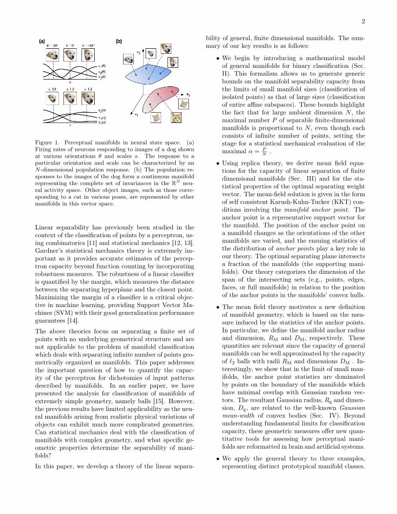
Each manifold Mµ ∈ RN is centered at xµ0 and consistsof a convex polytope with a finite number (2D) of ver-tices: {xµ0 ±Rkuµk , k = 1, ..., D}. The vectors uµi specifythe principal axes of the `1 ellipsoids. For simplicity, weconsider the case of `1 balls when all the radii are equal:Ri = R. We will concentrate on the cases when `1 ballsare high-dimensional; the case for `1 balls with D = 2was briefly described in [15]. The analytical expressionof the capacity is complex due to the presence of con-tributions from all types of supports, 1 ≤ k ≤ D + 1.We address important aspects of the high dimensionalsolution below.

15

High-dimensional `1 balls, scaling regime: In thescaling regime, we have ~v ≈ ~t. In this case, we can writethe solution for the subgradient as:

si(~t) =

{R sign (ti) , |ti| > |tj | ∀j 6= i

0 otherwise (50)

In other words, s(~t) is a vertex of the polytope corre-sponding to the component of ~t with the largest mag-nitude, see Fig. 5(c). The components of ~t are i.i.d.Gaussian random variables, and for large D, its maxi-mum component, tmax, is concentrated around

√2 logD.

Hence, Dg = 〈(s · ~t)2〉 = 〈t2max〉 = 2 logD which ismuch smaller than D. This result is consistent with thefact that the Gaussian mean width of a D-dimensional`1 ball scales with

√logD and not with D [22]. Since

all the points have norm R, we have Rg = R, andthe effective margin is then given by κg = R

√2 logD

, which is order unity in the scaling regime. In thisregime, the capacity is given by simple relation αM =α0

([κ+R

√2 logD

]/√

1 +R2).

High-dimensional `1 balls, R = O(1): When the ra-dius R is small as in the scaling regime, the only con-tributing solution is the touching solution (k = 1). WhenR increases, solutions with all values of k, 1 ≤ k ≤ D+ 1occur, and the support can be any face of the convexpolytope with dimension k. As R increases, the probabil-ity distribution p(k) over k of the solution shifts to largervalues. Finally, for large R, only two regimes dominate:fully supporting (k = D+1) with probability H (−κ) andpartially supporting with k = D with probability H(κ).

We illustrate the behavior of `1 balls with radius r andaffine dimension D = 100. In Fig. 9, (a) shows thelinear classification capacity as a function of r. Whenr → 0, the manifold approaches the capacity for isolatedpoints, αM ≈ 2, and when r → ∞, αM ≈ 1

D = 0.01.The numerical simulations demonstrate that despite thedifferent geometry, the capacity of the `1 polytope is sim-ilar to that of a `2 ball with radius RM and dimensionDM. In (b), for the scaling regime when r < 0.1 = 1√

D,

we see RM ≈ r, but when r � 1, RM is much smallerthan r, despite the fact that all Ri of the polytope areequal. This is because when r is not small, the variousfaces and eventually interior of the polytope contributeto the anchor geometry. In (c), we see DM ≈ 2 logD inthe scaling regime, while DM → D as r → ∞. In termsof the support structures, when r = 0.001 in the scalingregime (d1), most manifolds are either interior or touch-ing. For intermediate sizes (d2), the support dimensionis peaked at an intermediate value, and finally for verylarge manifolds (d3), most polytope manifolds are nearlyfully supporting.

R10-2 100 102

DM

0

50

100

r10-2 100 102

,M

0

0.5

1

1.5

2

L1balls(new)– (d1)canbeR=1e-2

R10-2 100 102

RM/R

0

0.2

0.4

0.6

0.8

(a) (b) (c)

!

2#$%!

Embedding dimension-1 0 1 2 3

Frac

tion

0

0.2

0.4

L1 balls, R=1.00e-03

Embedding dimension0 10 20 30 40

Frac

tion

0

0.02

0.04

0.06

0.08

L1 balls, R=2.50e+00

Embedding dimension90 95 100

Frac

tion

0

0.1

0.2

L1 balls, R=1.00e+02(d2) (d3)(d1)

& & &

ℓ(*+,,-, & = (0 − 2 ℓ(*+,,-, & = 3. 5 ℓ(*+,,-, & = (66

7 8/&

Support dimension (:) Supporting dimensionSupport dimension (:) Support dimension (:)

Figure 9. Separability of `1 balls. (a) Linear classificationcapacity of `1 balls as function of radius r with D = 100and N = 200: (blue) MFT solution, (black dashed) sphericalapproximation, (circle) full numerical simulations. (Inset) Il-lustration of `1 ball. (b) Manifold radius RM relative to theactual radius r. (c) Manifold dimensionDM as a function of r.In small r limit, DM is approximately 2 logD , while in larger, DM is close to D, showing how the solution is orthogonal tothe manifolds when their sizes are large. (d1-d3) Distributionof support dimensions: (d1) r = 0.001, where most mani-folds are either interior or touching, (d2) r = 2.5, where thesupport dimension has a peaked distribution, (d3) r = 100,where most manifolds are close to being fully supporting.

C. Smooth nonconvex manifolds: Ring manifolds

Many neuroscience experiments measure the responses ofneuronal populations to a continuously varying stimulus,with one or a small number of degrees of freedom. A pro-totypical example is the response of neurons in visual cor-tical areas to the orientation (or direction of movement)of an object. When a population of neurons respond bothto an object identity as well as to a continuous physicalvariation, the result is a set of smooth manifolds eachparameterized by a single variable, denoted θ, describingcontinuous curves in RN . Since in general the neural re-sponses are not linear in θ, the curve spans more than onelinear dimension. This smooth curve is not convex, andis endowed with a complex non-smooth convex hull. It isthus interesting to consider the consequences of our the-ory on the separability of smooth but non-convex curves.

The simplest example, considered here is the case where θcorresponds to a periodic angular variable such as orien-tation of an image, and we call the resulting non-convexcurve a ring manifold. We model the neuronal responsesas smooth periodic functions of θ, which can be parame-terized by decomposing the neuronal responses in Fouriermodes. Here, for each object, Mµ = xµ0 +

∑Di=1 siu

µi

where xµ0 represents the mean (over θ) of the popula-tion response to the object. The different D componentscorrespond to the different Fourier components of the an-

16

gular response, so that

s2n(θ) =Rn√

2cos(nθ) (51)

s2n−1(θ) =Rn√

2sin(nθ)

where Rn is the magnitude of the n-th Fourier componentfor 1 ≤ n ≤ D

2 . The neural responses in Eq. (1) aredetermined by projecting onto the basis:

uµi2n =√

2 cos(nθµi) (52)

uµi2n−1 =√

2 sin(nθµi)

The parameters θµi are the preferred orientation anglesfor the corresponding neurons and are assumed to beevenly distributed between −π ≤ θµi ≤ π (for simplicity,we assume that the orientation tuning of the neurons areall of the same shape and are symmetric around the pre-ferred angle). The statistical assumptions of our analysisassume that the different manifolds are randomly posi-tioned and oriented with respect to the others. For thering manifold model, this implies that the mean responsesxµ0 are independent random Gaussian vectors and alsothat the preferred orientation θµi angles are uncorrelated.With this definition, all the vectors ~s ∈ S obey the nor-malization ‖~s‖ = r where r2 =

∑D2n=1R

2n. Thus, for

each object the ring manifold is a closed non-intersectingsmooth curve residing on the surface of a D-dimensionalsphere with radius r .For the simplest case with D = 2, the ring manifoldis equivalent to a circle in two dimensions. However,for larger D, the manifold is not convex and its convexhull is composed of faces with varying dimensions. InFig. 10, we investigate the geometrical properties of thesemanifolds relevant for classification as a function of theoverall scale factor r, where for simplicity we have chosenRn = r for all n. The most striking feature is the smalldimension in the scaling regime, scaling roughly as Dg ≈2 logD. This logarithmic dependence is similar to that ofthe `1 ball polytopes. Then, as r increases, DM increasesdramatically from 2 logD to D.The similarity of the ring manifold to a convex poly-tope is also seen in the support dimension k of the man-ifolds. Support faces of dimension k 6= 0, 1, D + 1 areseen, implying the presence of partially supporting solu-tions. Interestingly, D2 < k ≤ D are excluded, indicatingthat the maximal face dimension of the convex hull is D

2 .Each face is the convex hull of a set of k ≤ D

2 pointswhere each point resides in the 2D subspace spanned bya pair of (real and imaginary) Fourier harmonics. Thering manifolds are closely related to the trigonometricmoment curve, whose convex hull geometrical propertieshave been extensively studied [27, 28].In conclusion, the smoothness of the convex hulls be-comes apparent in the distinct patterns of the support

2log(D)6 8 10 12

DM

6

8

10

12

r10-2 10-1 100 101 102

DM

0

5

10

15

20

r10-2 10-1 100 101 102

,

0

0.5

1

1.5

2

D=20, Uniform Rn

(d)(c)

(b)(a)

2!"#$r10-2 10-1 100 101 102

R M/r

0

0.2

0.4

0.6

0.8

1

%

k0 10 200

0.2

0.4

R = 0.01

k0 10 200

0.1

0.2

0.3

R = 20.00

k0 10 200

0.2

0.4

0.6R = 200.00

(e1) (e2) (e3)

Support dimension (k) Support dimension (k) Support dimension (k)

& = (. (* & = +( & = +((

Figure 10. Linear classification of D-dimensional ring mani-folds, with uniform Rn =

√2Dr. (a) Classification capacity

for D = 20 as function of r with m = 200 test samples (de-tails of numerical simulations in SM, Sec. S9): (blue) meanfield theory, (black dashed) spherical approximation, (blackcircles) numerical simulations. (Inset) Illustration of a ringmanifold. (b) Manifold dimension DM, which shows DM ∼ Din the large r limit, showing the orthogonality of the solution.(c) Manifold radius relative to the scaling factor r, RM

r, as

a function of r. Fact that RMr

becomes small implies thatthe manifolds are “fully supporting” to the hyperplane, show-ing the small radius structure. (d) Manifold dimension growswith affine dimension, D , as 2 logD for small r = 1

2√2 logD

in the scaling regime.(e1-e3) Distribution of support dimen-sions. (d1) r = 0.01, where most manifolds are either interioror touching, (d2) r = 20, where the support dimension hasa peaked distribution, truncated at D

2(d3) r = 200, where

most support dimensions are D2or fully supporting at D+ 1.

dimensions (compare Figs. 8(d) and 10(e)). However,we see that all manifolds with Dg ∼ 5 or larger sharecommon trends. As the size of the manifold increases,the capacity, and geometry vary smoothly, exhibiting asmooth cross-over from high capacity with low radius anddimension, to low capacity with large radius and dimen-sion. This crossover occurs as Rg ∝ 1/

√Dg. Also, our

examples demonstrate, in many cases when the size issmaller than the crossover value, the manifold dimen-sionality is substantially smaller than that expected fromnaive second order statistics, highlighting the saliency

17

and significance of our anchor geometry.

VI. MANIFOLDS WITH SPARSE LABELS

So far, we have assumed that the number of manifoldswith positive labels is approximately equal to the num-ber of manifolds with negative labels. In this section, weconsider the case where the two classes are unbalancedsuch that the number of positively-labeled manifolds isfar less than the negatively-labeled manifolds (the oppo-site scenario is equivalent). This is a special case of theproblem of classification of manifolds with heterogenousstatistics, where manifolds have different geometries orlabel statistics. We begin by addressing the capacity ofmixtures of manifolds and then focus on sparsely labeledmanifolds.

A. Mixtures of manifold geometries

Our theory of manifold classification is readily extendedto heterogeneous ensemble of manifolds, consisting of Ldistinct classes. In the replica theory, the shape of themanifolds appear only in the free energy term, G1 (seeAppendix, Eq. (A13)). For a mixture statistics, the com-bined free energy is given by simply averaging the indi-vidual free energy terms over each class l. Recall that thisfree energy term determines the capacity for each shape,giving an individual inverse critical load α−1

l . The inversecapacity of the heterogeneous mixture is then,

α−1 =⟨α−1l

⟩l

(53)

where the average is over the fractional proportions ofthe different manifold classes. This remarkably simplebut generic theoretical result enables analyzing diversemanifold classification problems, consisting of mixturesof manifolds with varying dimensions, shapes and sizes.Eq. (53) is adequate for classes that differ in their geome-try independent of the assigned labels. In general, classesmay differ in the label statistics (as in the sparse casestudied below) or in geometry that is correlated with la-bels. For instance, the positively labelled manifolds mayconsist of one geometry and the negatively labelled man-ifolds may have a different geometry. How do structuraldifferences between the two classes affect the capacity ofthe linear classification? A linear classifier can take ad-vantage of these correlations by adding a non-zero bias.Previously, it was assumed that the optimal separatinghyperplane passes through the origin; this is reasonablewhen the two classes are statistically the same. How-ever, when there are statistical differences between thelabel assignments of the two classes, Eq. (2) should be

replaced by yµ(w ·xµ− b) ≥ κ where the bias b is chosento maximize the mixture capacity, 53. The effect of opti-mizing the bias is discussed in detail in the next sectionfor the sparse labels and in other scenarios in SM (Sec.S3).

B. Manifolds with sparse labels

We define the sparsity parameter f as the fraction ofpositively-labeled manifolds so that f = 0.5 correspondsto having balanced labels. From the theory of the clas-sification of a finite set of random points, it is knownthat having sparse labels with f � 0.5 can drasticallyincrease the capacity [12]. In this section, we investigatehow the sparsity of manifold labels improves the manifoldclassification capacity.If the separating hyperplane is constrained to go throughorigin and the distribution of inputs is symmetric aroundthe origin, the labeling yµ is immaterial to the capacity.Thus, the effect of sparse labels is closely tied to having anon-zero bias. We thus consider inequality constraints ofthe form yµ(w·xµ−b) ≥ κ, and define the bias-dependentcapacity of general manifolds with label sparsity f , mar-gin κ and bias b, as αM(κ, f, b). Next, we observe thatthe bias acts as a positive contribution to the marginfor the positively-labeled population and as a negativecontribution to the negatively-labeled population. Thus,the dependence of αM(κ, f, b) on both f and b can beexpressed as,

α−1M (κ, f, b) ≡ fα−1

M (κ+ b) + (1− f)α−1M (κ− b) (54)

where αM(x) is the classification capacity with zero bias(and hence equivalent to the capacity with f = 0.5) forthe same manifolds. Note that Eq. (54) is similar to Eq.(53) for mixtures of manifolds. The actual capacity withsparse labels is given by optimizing the above expressionwith respect to b, i.e.,

αM(κ, f) = maxbαM(κ, f, b) (55)

In the following, we consider for simplicity the effect ofsparsity for zero margin, κ = 0.Importantly, if D is not large, the effect of the mani-fold geometry in sparsely labeled manifolds can be muchlarger than that for non-sparse labels. For non-sparse la-bels, the capacity ranges between 2 and (D+0.5)−1, whilefor sparse manifolds the upper bound can be much larger.Indeed, small-sized manifolds are expected to have ca-pacity that increases upon decreasing f as αM(0, f) ∝

1f |log f | , similar to P uncorrelated points [12]. This po-tential increase in capacity of sparse labels is howeverstrongly constrained by the manifold size, since when themanifolds are large, the solution has to be orthogonal tothe manifold directions so that αM(0, f) ≈ 1

D . Thus,

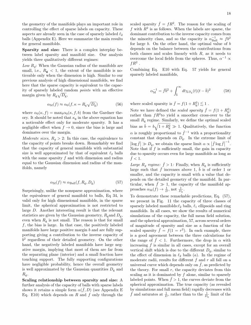
18

the geometry of the manifolds plays an important role incontrolling the effect of sparse labels on capacity. Theseaspects are already seen in the case of sparsely labeled `2balls (Appendix E). Here we summarize the main resultsfor general manifolds.Sparsity and size: There is a complex interplay be-tween label sparsity and manifold size. Our analysisyields three qualitatively different regimes:Low Rg: When the Gaussian radius of the manifolds aresmall, i.e., Rg < 1, the extent of the manifolds is no-ticeable only when the dimension is high. Similar to ourprevious analysis of high dimensional manifolds, we findhere that the sparse capacity is equivalent to the capac-ity of sparsely labeled random points with an effectivemargin given by Rg

√Dg,

αM(f) ≈ α0(f, κ = Rg√Dg) (56)

where α0(κ, f) = maxbα0(κ, f, b) from the Gardner the-ory. It should be noted that κg in the above equation hasa noticeable effect only for moderate sparsity. It has anegligible effect when f → 0, since the bias is large anddominates over the margin.Moderate sizes, Rg > 2: In this case, the equivalence tothe capacity of points breaks down. Remarkably we findthat the capacity of general manifolds with substantialsize is well approximated by that of equivalent `2 ballswith the same sparsity f and with dimension and radiusequal to the Gaussian dimension and radius of the man-ifolds, namely

αM(f) ≈ αBall(f,Rg, Dg) (57)

Surprisingly, unlike the nonsparse approximation, wherethe equivalence of general manifold to balls, Eq 34, isvalid only for high dimensional manifolds, in the sparselimit, the spherical approximation is not restricted tolarge D. Another interesting result is that the relevantstatistics are given by the Gaussian geometry, Rgand Dg,even when Rg is not small. The reason is that for smallf , the bias is large. In that case, the positively labeledmanifolds have large positive margin b and are fully sup-porting giving a contribution to the inverse capacity ofb2 regardless of their detailed geometry. On the otherhand, the negatively labeled manifolds have large neg-ative margin, implying that most of them are far fromthe separating plane (interior) and a small fraction havetouching support. The fully supporting configurationshave negligible probability, hence the overall geometryis well approximated by the Gaussian quantities Dg andRg.Scaling relationship between sparsity and size: Afurther analysis of the capacity of balls with sparse labelsshows it retains a simple form α(f , D) (see Appendix EEq. E10) which depends on R and f only through the

scaled sparsity f = fR2. The reason for the scaling off with R2 is as follows. When the labels are sparse, thedominant contribution to the inverse capacity comes fromthe minority class, and so the capacity is α−1

Ball ≈ fb2

for large b. On the other hand, the optimal value of bdepends on the balance between the contributions fromboth classes and scales linearly with R, as it needs toovercome the local fields from the spheres. Thus, α−1 ∝fR2 .Combining Eq. E10 with Eq. 57 yields for generalsparsely labeled manifolds,

α−1M = f b2 +

∫ ∞b

dtχDg(t)(t− b)2 (58)

where scaled sparsity is f = f(1 +R2g) . 1 .

Note we have defined the scaled sparsity f = f(1 + R2g)

rather than fR2to yield a smoother cross-over to thesmall Rg regime. Similarly, we define the optimal scaledbias as b = b

√1 +R2

g � 1. Qualitatively, the function

α is roughly proportional to f−1 with a proportionalityconstant that depends on Dg. In the extreme limit of∣∣log f

∣∣� Dg, we obtain the sparse limit α ∝∣∣f log f

∣∣−1.Note that if f is sufficiently small, the gain in capacitydue to sparsity occurs even for large manifolds as long asf < 1.Large Rg regime: f > 1: Finally, when Rg is sufficientlylarge such that f increases above 1, b is of order 1 orsmaller, and the capacity is small with a value that de-pends on the detailed geometry of the manifold. In par-ticular, when f � 1, the capacity of the manifold ap-proaches αM(f)→ 1

D , not 1Dg

.

To demonstrate these remarkable predictions, Eq. (57),we present in Fig. 11 the capacity of three classes ofsparsely labeled manifolds:`2 balls, `1 ellipsoids and ringmanifolds. In all cases, we show the results of numericalsimulations of the capacity, the full mean field solution,and the spherical approximation, 57, across several ordersof magnitude of sparsity and size as a function of thescaled sparsity f = f(1 = r2). In each example, thereis a good agreement between the three calculations forthe range of f < 1. Furthermore, the drop in α withincreasing f is similar in all cases, except for an overallvertical shift which is due to the different Dg, similar tothe effect of dimension in `2 balls (a). In the regime ofmoderate radii, results for different f and r all fall on auniversal curve which depends only on f , as predicted bythe theory. For small r, the capacity deviates from thisscaling as it is dominated by f alone, similar to sparselylabeled points. When f > 1, the curves deviate from thespherical approximation. The true capacity (as revealedby simulations and full mean field) rapidly decreases withf and saturates at 1

D , rather than to the 1Dg

limit of the

19

10-2 100 102 10410-2

10-1

100

101

102

10-4 10-2 100 10210-2

100

102

Sparsityforvariousmanifolds

(a)

!

D=10D=100

'( = 10)*

( = 10)+

( = 10),

( = 10)-

ℓ2 balls (c) (b)

/)-

Ring Manifolds ℓ1 Ellipsoids

0

((10-3 10-2 10-1 100 101

10-1

100

101

102

103 f=1e-04f=1e-03f=1e-02f=1e-01

( = 10)*

( = 10)+

( = 10),

( = 10)-

( = 10)+

( = 10),

( = 10)-

!

'

!

'

/1)-

Figure 11. (a-b) Classification of `2 balls with sparse labels:(a) Capacity of `2 balls as a function of f = f(1 + r2), forD = 100 (red) and D = 10 (blue): (solid lines) mean field the-ory, (dotted lines) is an approximation interpolating betweenEqs. 56 and 58 (details in SM, Sec. S9). (b–c) Classificationof general manifolds with sparse labels: (b) Capacity of `1ellipsoids with D = 100, where the first 10 components areequal to r, and the remaining 90 components are 1

2r, as a

function of f = (1 + R2g). r is varied from 10−3 to 103: (cir-

cles) numerical simulations, (lines) mean field theory, (dottedlines) spherical approximation. (c) Capacity of ring manifoldswith a Gaussian fall-off spectrum with σ = 0.1 and D = 100(; details in SM). Fig. 11(c) shows the capacity of ring mani-folds whose Fourier components have a Gaussian fall-off, i.e.Rn = A exp

[− 1

2(2π(n− 1)σ)2

].

spherical approximation. Finally, we note that our choiceof parameters in (c) (SM Section 7) were such that Rg(entering in the scaled sparsity) was significantly differentfrom simply an average radius. Thus, the agreement withthe theory illustrates the important role of the Gaussiangeometry in the sparse case.

As discussed above, in the (high and moderate) sparseregimes, a large bias alters the geometry of the two classesin different ways. To illustrate this important aspect, weshow in Fig. 12, the effect of sparsity and bias on thegeometry of the `1ellipsoids studied in Fig. 11(c). Herewe show the evolution of RM and DM for the majorityand minority classes as f increases. Note that despite thefact that the shape of the manifolds is the same for allf, their manifold anchor geometry depends on both classmembership and sparsity levels because these measuresdepend on the margin. When f is small, the minorityclass has DM = D as seen in Fig. 12(c), i.e., the minorityclass manifolds are close to be fully supporting due tothe large positive margin. This can also be seen in thedistributions of support dimension shown in Fig.12(a)-(b). On the other hand, the majority class has DM ≈Dg = 2logD1 � D, and these manifolds are mostly in theinterior regime. As f increases, the geometrical statisticsfor the two classes become more similar. This is seen inFig.12(c)-(d) where DM and RM for both majority andminority classes converge to the zero margin value forlarge f = f

(1 +R2

g).

20 40 600

0.05

0.1

0

0.2

0.4

0.6

0.8

0 5 95 100Support dimension (")

f(1+Rg2)

10-5 10-4 10-3 10-2 10-1 100

RM/R0

0

0.5

1

MinorMajor

f(1+Rg2)

10-5 10-4 10-3 10-2 10-1 100

DM

0

50

100

MinorMajor

Majority

f=$%&$ f=$%&'

Minority

Majority Minority

(a) (b)

(c) (d)

R )/r

f f

Support dimension (")

Figure 12. Manifold configurations and geometries for classi-fication of `1 ellipsoids with sparse labels, analyzed separatelyin terms of the majority and minority classes. The radii for`1 ellipsoids are Ri = r for 1 ≤ i ≤ 10 and Ri = 1

2r for

11 ≤ i ≤ 100 with r = 10. (a) Histogram of support di-mensions for moderate sparsity f = 0.1: (blue) minority and(red) majority manifolds. (b) Histogram of support dimen-sions for high sparsity f = 10−3: (blue) minority and (red)majority manifolds. (c) Manifold dimension as a function off = f(1 + R2

g) as f is varied: (blue) minority and (red) ma-jority manifolds. (d) Manifold radius relative to the scalingfactor r as a function of f : (blue) minority and (red) majoritymanifolds.

VII. SUMMARY AND DISCUSSION

Summary: We have developed a statistical mechanicaltheory for linear classification of inputs organized in per-ceptual manifolds, where all points in a manifold sharethe same label. The notion of perceptual manifolds iscritical in a variety of contexts in computational neuro-science modeling and in signal processing. Our theory isnot restricted to manifolds with smooth or regular geome-tries; it applies to any compact subset of aD-dimensionalaffine subspace. Thus, the theory is applicable to man-ifolds arising from any variation in neuronal responseswith a continuously varying physical variable, or fromany sampled set arising from experimental measurementson a limited number of stimuli.

The theory describes the capacity of a linear classifierto separate a dichotomy of general manifolds (with agiven margin) by a universal set of mean field equations.These equations may be solved analytically for simple ge-ometries, but for more complex geometries, we have de-veloped iterative algorithms to solve the self-consistentequations. The algorithms are efficient and converge fastas they involve only solving for O(D) variables of a sin-gle manifold, rather than invoking simulations of a full

20

system of P manifolds embedded in RN .Our theory provides for the first time, quantitative andqualitative predictions for the binary classification of re-alistic data structures. However, application to real datamay require further extensions of the theory as presentedhere. The most important ones (currently the subject ofon going work) include:Correlations: In the present work we have assumedthat the directions of the affine subspaces of the differ-ent manifolds are uncorrelated. In realistic situationswe expect to see correlations in the manifold geometries,mainly of two types: One is center-center correlations.Such correlations can be harmful for linear separabil-ity [29, 30]. Another is correlated variability in whichthe directions of the affine subspaces are correlated butnot the centers. Positive correlations of the latter formare beneficial for separability. In the extreme case whenthe manifolds share a common affine subspace, the rankof the union of the subspaces is Dtot = D rather thanDtot = PD, and the solution weight vector need only liein the null space of this smaller subspace. Further work isneeded to extend the present theory to incorporate moregeneral correlations.Generalization performance: We have studied theseparability of manifolds with known geometries. Inmany realistic problems, this information is not readilyavailable and only samples reflecting the natural variabil-ity of input patterns are provided. These samples can beused to estimate the underlying manifold model (usingmanifold learning techniques [31, 32]) and/or to train aclassifier based upon a finite training set. Generalizationerror describes how well a classifier trained on a finitenumber of samples would perform on other test pointsdrawn from the manifolds [33]. It would be importantto extend our theory to calculate the expected general-ization error achieved by the maximum margin solutiontrained on point cloud manifolds, as a function of the sizeof the training set and the geometry of the underlying fullmanifolds.Unrealizable classification: Throughout the presentwork, we have assumed that the manifolds are sepa-rable by a linear classifier. In realistic problems, theload may be above the capacity for linear separation,i.e. α > αM(κ = 0). Alternatively, neural noise maycause the manifolds to be unbounded in extent, with thetails of their distribution overlapping so that they arenot separable with zero error. There are several ways tohandle this issue in supervised learning problems. Onepossibility is to nonlinearly map the unrealizable inputsto a higher dimensional feature space, via a multi-layernetwork or nonlinear kernel function, where the classifi-cation can be performed with zero error. The design ofmultilayer networks could be facilitated using manifoldprocessing principles uncovered by our theory.Another possibility is to introduce an optimization prob-

lem allowing a small training error, for example, usingan SVM with complementary slack variables [14]. Theseprocedures raise interesting theoretical challenges, in-cluding understanding how the geometry of manifoldschange as they undergo nonlinear transformations, aswell as investigating by statistical mechanics, the perfor-mance of a linear classifier of manifolds with slack vari-ables [34].Concluding remarks: The statistical mechanical the-ory of perceptron learning has long provided a basis forunderstanding the performance and fundamental limita-tions of single layer neural architectures and their kernelextensions. However, the previous theory only consid-ered a finite number of random points with no underly-ing geometric structure, and could not explain the per-formance of linear classifiers on large, possibly infinitenumber of inputs organized as distinct manifolds by thevariability due to changes in physical parameters of ob-jects. The statistical mechanical theory presented in thiswork can explain the capacity and limitations of linearclassification of general manifolds, and be used to eluci-date changes in neural representations across hierarchi-cal sensory systems. We believe the application of thistheory and its corollary extensions will precipitate novelinsights into how perceptual systems, biological or artifi-cial, can efficiently code and process sensory information.We would like to thank Uri Cohen, Ryan Adams, LeslieValiant, David Cox, Jim DiCarlo, Doris Tsao, and YoramBurak for helpful discussions. The work is partially sup-ported by the Gatsby Charitable Foundation, the SwartzFoundation, the Simons Foundation (SCGB Grant No.325207), the NIH, and the Human Frontier Science Pro-gram (Project RGP0015/2013). D. D. Lee also acknowl-edges the support of the US National Science Foundation,Army Research Laboratory, Office of Naval Research, AirForce Office of Scientific Research, and Department ofTransportation.

Appendix A: Replica Theory of Manifold Capacity

In this section, we outline the derivation of the meanfield replica theory summarized in Eqs. (11)-12. Wedefine the capacity of linear classification of manifolds,αM(κ), as the maximal load, α = P

N , for which withhigh probability a solution to yµw · xµ ≥ κ exists fora given κ. Here xµ are points on the P manifolds Mµ,Eq. (1), and we assume that all NP (D+ 1) componentsof {uµi } are drawn independently from a Gaussian dis-tribution with zero mean and variance 1

N , and that thebinary labels yµ = ±1 are randomly assigned to eachmanifold with equal probabilities. We consider the ther-modynamic limit where N, P → ∞ but α = P

N , and Dare finite.Note that the geometric margin, κ′, defined as the dis-

21

tance from the solution hyperplane is given by yµw ·xµ ≥κ′ ‖w‖ = κ′

√N . However, this distance depends on the

scale of the input vectors xµ. The correct scaling of themargin in the thermodynamic limit is κ′ = ‖x‖√

Nκ. Since

we adopted the normalization of ‖xµ‖ = O(1), the cor-rect scaling of the margin is yµw · xµ ≥ κ .

Evaluation of solution volume: Following Gardner’sreplica framework, we first consider the volume Z of thesolution space for α < αM(κ) . We define the signed pro-jections of the the ith direction vector uµi on the solutionweight as Hµ

i =√Nyµw · uµi , where i = 1, ..., D + 1 and

µ = 1, ..., P . Then, the separability constraints can bewritten as

∑D+1i=1 SiH

µi ≥ κ . Hence the volume can be

written as

Z =

∫dNwδ(w2 −N) ΠP

µ=1Θµ

(gS( ~Hµ)− κ

)(A1)

where Θ(x) is a Heaviside step function. gS is thesupport function of S defined for Eq. 12 as gS(~V ) =

min~S

{~V · ~S | ~S ∈ S

}.

The volume defined above depends on the the quenchedrandom variables uµi and yµ throughHµ

i . It is well knownthat in order to obtain the typical behavior in the thermo-dynamic limit, we need to average logZ, which we carryout using the replica trick, 〈logZ〉 = limn→0

〈Zn〉−1n ,

where 〈〉 refers to the average over uµi and yµ. For naturaln, we need to evaluate,

〈Zn〉 =

∫ n∏α

dwαδ(w2α −N)

P∏µ

∫D ~Hµα (A2)

〈D+1∏i

√2πδ(Hµα

i − yµwTαuµi )〉uµi ,yµ

where we have used the notation,

D ~H = ΠD+1i=1

dHi√2π

Θ(gS( ~H)− κ

)(A3)

Using Fourier representation of the delta functions, weobtain

〈Zn〉 =

∫ n∏α

dwαδ(w2α −N)

P∏µ

∫D ~Hµα (A4)

D+1∏i=1

∫dHµα

i√2π

⟨exp

{iHµα

i (Hµαi − yµwT

αuµi )}⟩

uµi ,yµ

Performing the average over the Gaussian distributionof uµi (each of the N components has zero mean and

variance 1N ) yields,⟨

expD+1∑i=1

∑µα

iHµαi (−yµ

N∑j=1

wjαuµi,j)

⟩uµi ,y

µ

(A5)

= exp

−1

2

∑αβ

qαβ∑iµ

Hµαi Hµβ

i

where, qαβ = 1

N

∑Nj=1 w

jαw

jβ . Thus, integrating the vari-

ables Hµαi yields

〈Zn〉 =

∫ n∏α=1

dwαδ(w2α −N)

∫dqαβΠαβ (A6)

· δ(Nqαβ −wT

αwβ

) [exp

(− (D + 1)

2logdetq

)X

]Pwhere

X =

∫ ∏α

D ~Hα exp

−1

2

∑i,α,β

Hαi (q−1)αβH

βi

(A7)

and we have used the fact that all manifolds contributethe same factor.We proceed by making the replica symmetric ansatz onthe order parameter qαβ at its saddle point, qαβ = (1 −q)δαβ + q, from which one obtains in the n→ 0 limit:

q−1αβ =

1

1− q δαβ −q

(1− q)2(A8)

and

logdetq = n log(1− q) +nq

1− q (A9)

Thus the exponential term in X can be written as

exp

−1

2

∑αi

(Hαi )

2

1− q +1

2

∑i

( √q

1− q∑α

Hαi

)2 (A10)

Using the Hubbard–Stratonovich transformation, we ob-tain

X =

∫D~T

[∫D ~H exp

{−1

2

~H2

1− q +

√q

1− q~H · ~T

}]n(A11)

where D~T = ΠidTi√

2πexp

(−T

2i

2

). Completing the

square in the exponential and using∫D~TAn =

expn∫D~T logA in the n → 0 limit, we obtain, X =

exp(nq(D+1)2(1−q) + n

∫D~T log z(~T )

)with

z(~T ) =

∫D ~H exp

{− 1

2(1− q) ||~H −√q ~T ||2

}(A12)

22

Combining these terms, we write the last factor in Eq.(A6) as expnPG1 where,

G1 =

∫D~T log z(~T )− (D + 1)

2log(1− q) (A13)

The first factors in 〈Zn〉, Eq. (A6), can be written asexpnNG0, where as in the Gardner theory, the entropicterm in the thermodynamic limit is

G0(q) =1

2ln(1− q) +

q

2(1− q) (A14)

and represents the constraints on the volume of wαdueto normalization and the order parameter q. Combiningthe G0 and G1contributions, we have

〈Zn〉t0,t = eNn[G0(q)+αG1(q)] (A15)

The classification constraints contribute αG1, with Eq.(A13), and

z(~T ) =

∫ΠD+1i=1

dYi√2π(1− q)

exp

(−

~Y 2

2(1− q)

)(A16)

Θ(gS(√q ~T + ~Y )− κ

)where, we have written the fields Hi as

Hi =√qTi + Yi (A17)

Note that √qTi represents the quenched random com-ponent due to the randomness in the uµi , and Yi is the“thermal” component due to the variability within thesolution space. The order parameter q is calculated via0 = ∂G0

∂q + α∂G1

∂q .

Capacity: In the limit where α → αM(κ) , the over-lap between the solutions become unity and the volumeshrinks to zero. It is convenient to define Q = q

1−q andstudy the limit of Q→∞. In this limit the leading orderis

〈logZ〉 =Q

2

[1− α〈F (~T )〉~T

](A18)

where the first term is the contribution from G0 → Q2 .

The second term comes from G1 → −Q2 α〈F (~T )〉~T , wherethe average is over the Gaussian distribution of the D+1dimensional vector ~T , and

F (~T )→ − 2

Qlog z(~T ) (A19)

is independent ofQ and is given by replacing the integralsin Eq. (A16) by their saddle point, which yields

F (~T ) = min~V

{∥∥∥~V − ~T∥∥∥2

| gS(~V)− κ ≥ 0

}(A20)

At the capacity, logZ vanishes, the capacity of a generalmanifold with margin κ, is given by,

α−1M (κ) = 〈F (~T )〉~T (A21)

F (~T ) = min~V

{∥∥∥~V − ~T∥∥∥2

| gS(~V )− κ ≥ 0

}(A22)

Finally, we note that the mean squared ’annealed’ vari-ability in the fields due to the entropy of solutions van-ishes at the capacity limit, as 1/Q , see Eq. (A16) . Thus,

the quantity∥∥∥~V − ~T

∥∥∥2

in the above equation representsthe annealed variability times Q which remains finite inthe limit of Q→∞.

Appendix B: Strictly Convex Manifolds

B.1. General

Here we evaluate the capacity of strictly convex mani-folds, starting from the expression for general manifolds,Eq. 21. In a strictly convex manifold, S , any point inthe line segment connecting two points ~x and ~y, ~x, ~y ∈ S, other than ~x and ~y, belongs to the interior of S . Thus,the boundary of the manifold does not contain edges orflats with spanning dimension k > 1 except of the en-tire manifold, k = D + 1 . Therefore, there are exactlycontributions to the inverse capacity. When t0 obeysttouch(~t) > t0 − κ > tfs(~t), the integrand of Eq. 21 con-tributes (−~t·s(~T )−t0+κ)2

1+‖s(~T )‖2 , When t0 < κ+ tfs(~t), the man-

ifold is fully embedded. In this case, ~v = 0, and theintegrand reduces to Eq. 27. In summary, the capacityfor convex manifolds can be written as

α−1(κ) =

∫D~t

∫ κ+ttouch(~t)

κ+tfs(~t)

Dt0(−~t · s(~t, t0)− t0 + κ)2

1 +∥∥s(~t, t0)

∥∥2

(B1)

+

∫D~t

∫ κ+tfs(~t)

−∞Dt0

[(t0 − κ)

2+∥∥~t∥∥2

]

where ttouch(~t) and tfs(~t) are given by Eqs. 23 and 26,respectively, and s(~t, t0) = arg min~s(~v · ~s), with ~v = ~t +(v0 − t0)s.

B.2. `2 Balls

In the case of `2 balls with D and radius R, g(~v) =−R ‖~v‖ . Hence, ttouch(~t) = R

∥∥~t∥∥ and tfs(~t) = −R−1∥∥~t∥∥

23

. Thus, Eq. B1 reduces to hat the capacity of balls is

α−1Ball =

∫ ∞0

dtχD(t)

∫ κ+tR

κ−tR−1

Dt0(−t0 + tR+ κ)2

(1 +R2)

+

∫ ∞0

dtχD(t)

∫ κ−tR−1

−∞Dt0

[(t0 − κ)2 + t2

](B2)

where,

χD(t) =21−D2

Γ(D2 )tD−1e−

12 t

2

, t ≥ 0 (B3)

is the D-dimensional Chi probability density function,reproducing the results of [15]. Furthermore, Eq. B2 canbe approximated by the capacity of points with a marginincrease of R

√D, i.e. αBall (κ,RM, DM) ≈ (1+R2)α0(κ+

R√D) (details in [15]).

B.2. `2 Ellipsoids

a. Anchor points and support regimes

With ellipsoids, Eq. 36, the support function in Eq. 15can be computed explicitly as follows. For a vector ~V =(~v, v0), with non zero ~v, the support function g(~v) isminimized by a vector ~s which occurs on the boundary ofthe ellipsoid, i.e. it obeys the equality constraint f(~s) = 0

with ρ(~s) =∑Di=1

(siRi

)2

− 1 , Eq. (36). To evaluate g,

we differentiate −∑Di=1 si~vi + ρf(~s) with respect to ~si,

where ρ is a Lagrange multiplier enforcing the constraint,yielding

si = −viR2i

g(~v)(B4)

and

g(~v) = −∥∥∥~v ◦ ~R∥∥∥ (B5)

where ~R is the D dimensional vector of the ellipsoid prin-cipal radii, and we denote ◦refers to pointwise product ofvectors, (~v ◦ ~R)i = viRi. For a given (~t, t0), the vector(~v, v0) is determined by Eq. (13) and the analytic solu-tion above can be used to derive explicit expressions fors(~t, t0) in the different regimes as follows.Interior regime:In the interior regime λ = 0 , ~v = ~t, resulting in zerocontribution to the inverse capacity. The anchor pointis given by the following boundary point on the ellipse,given by Eq. B4 with ~v = ~t. This regime holds for t0

obeying the inequality t0 − κ ≥ ttouch(~t) with Eq. 23,yielding

ttouch(~t) =∥∥∥~t ◦ ~R∥∥∥ (B6)

Touching regime: Here the anchor point is given by Eq.B4 where ~v = ~t + λs. Substituting ti + λsi for vi in thenumerator of that equation, and g(~v) = κ−v0 = κ−t0−λ, yields,

stouch,i(~t, t0) = − tiR2i

λ(1 +R2i ) + (−t0 + κ)

, (B7)

where the parameter λ is determined by the ellipsoidalconstraint,

1 =

D∑i=1

t2iR2i

[λ(1 +R2i ) + (−t0 + κ)]

2 . (B8)

In this regime, the contribution to the capacity is givenby Eq. 16-17 with s in Eq. (B7).The touching regime holds for ttouch > t0 − κ > tfs ,where λ → κ − t0 , ~v vanishes, and the anchor point isthe point on the boundary of the ellipsoid antiparallel to~t . Substituting this value of λ in Eq. B8 , yields,

tfs(~t) = −

√√√√∑i

(tiRi

)2

(B9)

Fully supporting regime: When t0−κ < tfs , we have~v = 0, v0 = κ, and λ = t0 − κ, implying that the centeras well as the entire ellipsoid is fully supporting the maxmargin solution. In this case, the anchor point is antipar-allel to ~t at the interior point, 25, and its contribution tothe capacity is as in Eq. 27.

Appendix C: Limit of Large Manifolds

In the large size limit, ‖s‖ → ∞ , linear separationof manifolds reduces to linear separation of P randomD-dimensional affine subspaces. When separating sub-spaces, all of them must be fully embedded in the mar-gin plane, otherwise they would intersect it and violatethe classification constraints. However, the way large sizemanifolds approach this limit is subtle. To analyze thislimit, we note that when ‖s‖ is large, g(~v) < ‖s‖ ‖~v‖ andfrom the condition that g(~v) ≥ (−v0 +κ), we have ‖~v‖ ≤(−v0+κ)‖s‖ , i.e., ‖~v‖ is O(‖s‖−1

). A small ‖~v‖ implies thatthe affine basis vectors, except the center direction, are alleither exactly or almost orthogonal to the solution weightvector. Since λs = −~t+~v ≈ −~t, it follows that s is almostantiparallel to the gaussian vector ~t, hence DM → D, see

24

Eq. 30. To elucidate the manifold support structure,we note first that by Eq. 23 ttouch ∝ −||~t||||s|| → −∞hence the fractional volume of the interior regime is neg-ligible, and the statistics is dominated by the embed-ded regimes. In fact, the fully embedded transition isgiven by tembed ≈ −κ , see Eq.26, so that the frac-tional volume of the fully embedded regime is H(−κ) =∫∞−κDt0 and its contribution to inverse capacity is there-

fore∫∞−κDt0

[〈∥∥~t∥∥2〉+ (t0 + κ)2

]= H(−κ)D + α−1

0 (κ) .The remaining summed probability of the touching andpartially embedded regimes (k ≥ 1) is therefore H(κ).In these regimes, λ2 ‖s‖2 ≈ λ2 ‖s‖2 ≈

∥∥~t∥∥2, so that this

regime contributes a factor of∫ −κ−∞Dt0〈

∥∥~t∥∥2〉 = H(κ)D.Combining these two contributions, we obtain for largesizes, α−1

M = D + α−10 (κ), consistent with Eq. (8).

Appendix D: High Dimensional Manifolds

D.1. High Dimensional `2 ball

Before we discuss general manifolds in high dimension,we focus on the simple case of high dimensional balls,the capacity of which is given by Eq. B2. When D � 1, χD(t) , B3, is centered around t =

√D. Substituting

χD(t) ≈ δ(t−√D) yields

α−1Ball(κ,R,D) =

∫ κ+R√D

κ−√DR

Dt0(R√D + κ− t)2

0

R2 + 1+

∫ κ−√DR

−∞Dt0([t0−κ]2+D)

(D1)As long as R �

√D , the second term in Eq. (D1)

vanishes and yields

α−1Ball(κ,R,D) =

∫ κ+R√D

−∞Dt0

(R√D + κ− t0)2

R2 + 1(D2)

Here we note that the t0 term in the numerator is signif-icant only if R = O(D−1/2) or smaller, in which case thedenominator is just 1 . When R is of order 1 the termt0 in the integrand is negligible. Hence, in both cases wecan write,

α−1Ball(κ,R,D) ≈ α−1

0

(κ+R

√D√

1 +R2

)(D3)

In this form, the intuition beyond the factor√

1 +R2

is clear, stemming from the fact that the distance of apoint from the margin plane scales with its norm, hencethe margin entering the capacity should factor out thisnorm.

As stated above, Eq, D3 implies a finite capacity only inthe scaling regime, where R

√D = O(1). If, on the other

hand, R√D � 1, Eq. (D2) implies

α−1Ball =

R2D

1 +R2(D4)

(where we have used the asymptote α−10 (x) → x2 for

large x), reducing to α−1 = D for large R.The analysis above also highlights the support structureof the balls at large D. As long as R�

√D the

fraction of balls that lie fully in the margin plane, is neg-ligible, as implied by the fact that tsf ≈ −

√D/R →

−∞.The overall fraction of interior balls is H(κ+R√D)

whereas the fraction that touch the margin planes is1 − H(κ + R

√D) . Despite the fact that there are no

fully supporting balls, the touching balls are almost par-allel to the margin planes if R � 1 hence the capacityreaches its lower bound.Finally, the large manifold limit discussed in AppendixC is realized for as R �

√D . Here, tsf = −κ and

the system is either touching or fully supporting withprobabilities H(κ) and H(−κ), respectively.

D.2. General manifolds.

To analyze the limit of large dimensional general mani-folds we utilize the self averaging of terms in Eq. (21),involving sums of the D components of ~t and s, i.e.,

~t · s ≈ 〈||s||〉〈~t · s〉 ≈ RM√DM = κM

(D5)

Also, ttouch ≈ ~t · s ≈ κM , hence, we obtain for the capac-ity,

α−1M (κ) ≈ 〈[κM + κ− t0]2+〉t0

R2M + 1

≈ α−1Ball(κ,RM, DM) (D6)

where the average is wrt the gaussian t0. Evaluating RMand DM involves calculations of the self consistent statis-tics of the anchor points. This calculation is simplifiedin high dimension. In particular, λ, Eq. 17 , reduces to

λ ≈ 〈[κM + κ− t0]+〉t01 +R2

M(D7)

hence it is approximately constant, independent of ~T .In deriving the above approximations we used self-averaging in summations involving theD intrinsic coordi-nates. The full dependence on the longitudinal gaussian

25

t0 should remain. Thus, RMand DM should in fact besubstituting by RM(t0) and DM(t0) denoting 29-30 withaveraging only over ~t. This would yield a more compli-cated expressions than Eq.D6- D7.

The reason why we can replace them by average quan-tities is the following: the potential dependence of theanchor radius and dimension on t0 is via λ(t0). However,inspecting Eq. D7 we note two scenarios: One in whichRM is small and κM of order 1 . In this case, becausethe manifold radius is small the contribution λs is smalland can be neglected. This is the same argument why inthis case, the geometry can be replaced by the Gaussiangeometry which does not depend on t0 or κ . The secondscenario is that RM is of order 1 and κM � 1, in whichcase the order 1 contribution from t0 is negligible.

Appendix E: Capacity of `2 Balls with Sparse Labels

We begin by writing the capacity of random points withsparse labels [12], as α0(f, κ) = maxbα0(f, κ, b), where

First, we note that the capacity of sparsely labeled pointsis α0(f, κ) = maxbα0(f, κ, b), where

α−10 (f, κ, b) = f

∫ κ+b

−∞Dt(−t+ κ+ b)2

+ (1− f)

∫ κ−b

−∞Dt(−t+ κ− b)2 (E1)

Optimizing b yields the following equation for b,

0 = f

∫ b+κ

−∞Dt(−t+κ+ b) + (1−f)

∫ b−κ

−∞Dt(−t+κ− b)

(E2)

In the limit of f → 0, b� 1 . The first equation reducesto

α−10 ≈ fb2 + exp

(−b2/2

)(E3)

yielding for the optimal b ≈√

2| log f | . With this b, theinverse capacity is dominated by the first term which isα−1

0 ≈ 2f | log f | .

The capacity for `2 balls of radius R with sparse labels

with sparsity f (Eq. (54) and Eq. B2) is given by,

α−1Ball = f

∫ ∞0

dtχD(t)x[∫ κ+tR+b

κ−tR−1+b

Dt0(−t0 + tR+ b+ κ)2

(1 +R2)

+

∫ b+κ−tR−1

−∞Dt0((t0 − b− κ)2 + t2)

]

+ (1− f)

∫ ∞0

dtχD(t)x[∫ κ+tR−b

κ−tR−1−bDt0

(−t0 + tR+ κ− b)2

(1 +R2)

+

∫ −b+κ−tR−1

−∞Dt0((t0 − κ+ b)2 + t2)

](E4)

and the optimal bias b is given by ∂αB/∂b = 0. Here weanalyze these equations in various size regimes assumingκ = 0.Small R: For balls with small radius, the capacity isthat of points, unless the dimensionality is high. Thus,if D is large but R

√D . 1,

α−1Ball = f

∫ R√D+b

−∞Dt0

(−t0 +R√D + b)2

(1 +R2)

+ (1− f)

∫ R√D−b

−∞Dt0

(−t0 +R√D + b)2

(1 +R2)

(E5)

that is,

αBall(f,R,D) ≈ α0(f, κ = R√D) (E6)

As noted above when f → 0 the optimal bias di-verges, hence the presence of order 1 the induced mar-gin is noticeable only for moderate f such that R

√D =

O(| log f |).Small f and large R: Here we analyze the above equa-tions in the limit of small f and large R. We assume thatf is sufficiently small so that the optimal bias b is large.The contribution of the minority class to the inverse ca-pacity α−1

B is dominated by

f

∫ ∞0

dtχD(t)

∫ b

−∞Dt0((−t0 + b)2 + t2) ≈ fb2 (E7)

The dominant contribution of the majority class to α−1B

is,

26

(1− f)

∫ ∞0

dtχD(t)

∫ −b+tR−b−Rt−1

Dt0(−t0 + tR− b)2

(1 +R2)(E8)

≈ (1− f)

∫ ∞b

dtχD(t)(t− b)2 (E9)

where b = b/R . In deriving the last equation we used(−t0+tR−b)2

(1+R2) → (t−b)2as R, b→∞ . Second, the integralsare of substantial value only if t ≥ b in which case theintegral of t0 is

∫ b−R(b−t)Dt0 ≈ 1 and the integral over

t is from b to ∞. Combining the two results yields thefollowing simple expression for the inverse capacity,

α−1Ball = f b2 +

∫ ∞b

dtχD(t)(t− b)2 (E10)

where scaled sparsity is f = fR2. The optimal scaledbias is given by,

f b =

∫ ∞b

dtχD(t)(t− b) (E11)

Note that R and f affect the capacity only through thescaled sparsity. When f → 0, capacity is proportionalto (f | log f |)−1. In a realistic regime of small f (between10−4to 1) capacity decreases with f roughly as 1/f witha proportionality constant which depends onD, as shownin the examples of Fig. 12 (a). Finally, when R is suffi-ciently large that f > 1, b is order 1 or smaller. In thiscase, the second term in Eq. E10 dominates and con-tributes 〈t2〉 = D yielding a capacity that saturates asD−1 as shown in Fig. 11(a). It should be noted how-ever, that when b is not large, the approximations Eq.E10-E11 don’t hold anymore.

[1] James J DiCarlo and David D Cox. Untangling in-variant object recognition. Trends in cognitive sciences,11(8):333–341, 2007.

[2] Jennifer K Bizley and Yale E Cohen. The what, whereand how of auditory-object perception. Nature ReviewsNeuroscience, 14(10):693–707, 2013.

[3] Kevin A Bolding and Kevin M Franks. Complementarycodes for odor identity and intensity in olfactory cortex.eLife, 6:e22630, 2017.

[4] H Sebastian Seung and Daniel D Lee. The manifold waysof perception. Science, 290(5500):2268–2269, 2000.

[5] James J DiCarlo, Davide Zoccolan, and Nicole C Rust.How does the brain solve visual object recognition? Neu-ron, 73(3):415–434, 2012.

[6] Ben Poole, Subhaneil Lahiri, Maithreyi Raghu, JaschaSohl-Dickstein, and Surya Ganguli. Exponential expres-sivity in deep neural networks through transient chaos.

In Advances In Neural Information Processing Systems,pages 3360–3368, 2016.

[7] Marc Aurelio Ranzato, Fu Jie Huang, Y-Lan Boureau,and Yann LeCun. Unsupervised learning of invariantfeature hierarchies with applications to object recogni-tion. In Computer Vision and Pattern Recognition, 2007.CVPR’07. IEEE Conference on, pages 1–8. IEEE, 2007.

[8] Yoshua Bengio. Learning deep architectures for ai. Foun-dations and trends R© in Machine Learning, 2(1):1–127,2009.

[9] Ian Goodfellow, Honglak Lee, Quoc V Le, Andrew Saxe,and Andrew Y Ng. Measuring invariances in deep net-works. In Advances in neural information processing sys-tems, pages 646–654, 2009.

[10] Charles F Cadieu, Ha Hong, Daniel LK Yamins, NicolasPinto, Diego Ardila, Ethan A Solomon, Najib J Majaj,and James J DiCarlo. Deep neural networks rival therepresentation of primate it cortex for core visual objectrecognition. PLoS Comput Biol, 10(12):e1003963, 2014.

[11] Thomas M Cover. Geometrical and statistical propertiesof systems of linear inequalities with applications in pat-tern recognition. IEEE transactions on electronic com-puters, (3):326–334, 1965.

[12] Elizabeth Gardner. The space of interactions in neuralnetwork models. Journal of physics A: Mathematical andgeneral, 21(1):257, 1988.

[13] E. Gardner. Maximum storage capacity in neural net-works. EPL (Europhysics Letters), 4(4):481, 1987.

[14] Vladimir Vapnik. Statistical learning theory. Wiley NewYork, 1998.

[15] SueYeon Chung, Daniel D Lee, and Haim Sompolinsky.Linear readout of object manifolds. Physical Review E,93(6):060301, 2016.

[16] Stephen Boyd and Lieven Vandenberghe. Convex opti-mization. Cambridge university press, 2004.

[17] Ralph Tyrell Rockafellar. Convex analysis. Princetonuniversity press, 2015.

[18] Jean-Jacques Moreau. Décomposition orthogonale d’unespace hilbertien selon deux cônes mutuellement polaires.CR Acad. Sci. Paris, 225:238–240, 1962.

[19] SueYeon Chung, Uri Cohen, Haim Sompolinsky, andDaniel D Lee. Learning data manifolds with a cuttingplane method. Neural Computation (Accepted), 2018.

[20] Branko Grünbaum and Geoffrey C Shephard. Convexpolytopes. Bulletin of the London Mathematical Society,1(3):257–300, 1969.

[21] AA Giannopoulos, VDMilman, and M Rudelson. Convexbodies with minimal mean width. In Geometric aspectsof functional analysis, pages 81–93. Springer, 2000.

[22] Roman Vershynin. Estimation in high dimensions: a ge-ometric perspective. In Sampling theory, a renaissance,pages 3–66. Springer, 2015.

[23] Kanaka Rajan, LF Abbott, and Haim Sompolinsky.Stimulus-dependent suppression of chaos in recurrentneural networks. Physical Review E, 82(1):011903, 2010.

[24] Ashok Litwin-Kumar, Kameron Decker Harris, RichardAxel, Haim Sompolinsky, and LF Abbott. Optimal de-grees of synaptic connectivity. Neuron, 93(5):1153–1164,2017.

[25] Jia Deng, Wei Dong, Richard Socher, Li-Jia Li, Kai Li,and Li Fei-Fei. Imagenet: A large-scale hierarchical im-age database. In Computer Vision and Pattern Recog-nition, 2009. CVPR 2009. IEEE Conference on, pages248–255. IEEE, 2009.

27

[26] Christian Szegedy, Wei Liu, Yangqing Jia, Pierre Ser-manet, Scott Reed, Dragomir Anguelov, Dumitru Er-han, Vincent Vanhoucke, and Andrew Rabinovich. Goingdeeper with convolutions. In Proceedings of the IEEEConference on Computer Vision and Pattern Recogni-tion, pages 1–9, 2015.

[27] Seung-Hyeok Kye. Faces for two qubit separable statesand the convex hulls of trigonometric moment curves.arXiv preprint arXiv:1302.2226, 2013.

[28] Zeev Smilansky. Convex hulls of generalized momentcurves. Israel Journal of Mathematics, 52(1):115–128,1985.

[29] Rémi Monasson. Properties of neural networks stor-ing spatially correlated patterns. Journal of Physics A:Mathematical and General, 25(13):3701, 1992.

[30] B Lopez, M Schroder, and M Opper. Storage of corre-

lated patterns in a perceptron. Journal of Physics A:Mathematical and General, 28(16):L447, 1995.

[31] Sam T Roweis and Lawrence K Saul. Nonlinear dimen-sionality reduction by locally linear embedding. Science,290(5500):2323–2326, 2000.

[32] Joshua B Tenenbaum, Vin De Silva, and John C Lang-ford. A global geometric framework for nonlinear dimen-sionality reduction. science, 290(5500):2319–2323, 2000.

[33] Shun-ichi Amari, Naotake Fujita, and Shigeru Shi-nomoto. Four types of learning curves. Neural Com-putation, 4(4):605–618, 1992.

[34] Sebastian Risau-Gusman and Mirta B Gordon. Statis-tical mechanics of learning with soft margin classifiers.Physical Review E, 64(3):031907, 2001.