Class Notes Fall 2020 - user.engineering.uiowa.edu

ME:5160 Chapter 1

Professor Fred Stern Fall 2020 1

ME:5160

Intermediate Mechanics of Fluids

Class Notes

Fall 2020

Prepared by:

Professor Fred Stern

Typed by:

Derek Schnabel (Fall 2004)

Nobuaki Sakamoto (Fall 2006)

Hamid Sadat-Hosseini (Fall 2006)

Maysam Mousaviraad (Fall 2006)

Corrected by:

Jun Shao (Fall 2004)

Mani Kandasamy (Fall 2005)

Tao Xing, Hyun Se Yoon (Fall 2006)

Hamid Sadat-Hosseini (Fall 2007-2010)

Maysam Mousaviraad (Fall 2013-2016)

Timur Kent Dogan (Fall 2017-2018)

Sungtek Park (Fall 2019-2020)

ME:5160 Chapter 1


Chapter 1: Introduction Definition of a fluid:

A fluid cannot resist an applied shear stress and remain

at rest, whereas a non-fluid (i.e., solid) can.

Solids resist shear by static deformation up to an

elastic limit of the material, after which they undergo

fracture.

Fluids deform continuously (undergo motion) when

subjected to shear stress. Consider a fluid between two

parallel plates, with the lower one fixed and the upper

moving at speed U, which is an example of Couette flow

(i.e, wall/shear driven flows)

𝑉 = 𝑢(𝑦) 𝑖 𝑑𝑢(𝑦)

𝑑𝑦=

𝑈

ℎ

1-D flow velocity

profile

u(y)

x

y

u=0

u=U

h

ME:5160 Chapter 1


No slip condition:

Length scale of molecular mean free path λ << length scale

of fluid motion ℓ; therefore, macroscopically there is no

relative motion or temperature between the solid and fluid

in contact.

Knudsen number = Kn = λ/ℓ << 1

Exceptions are rarefied gases and gas/liquid contact line.

Newtonian fluids:

Rate of Strain:

(u+uy dy)dt

x

y

dy dӨ = tan-1 uydt

Fluid element with sides parallel to the

coordinate axes at time t=0.

Fluid element deformation at

time t + dt

y

x

dy

u+uydy

u

u dt

ME:5160 Chapter 1


dy

dydtud

ytan yu

dt

d

.

dy

du

.

(rate of strain = velocity gradient)

For 3D flow, rate of strain is a second order symmetric

tensor: 1

2

jiij

j i

uu

x x

= εji

Diagonal terms are elongation/contraction in x,y,z and off

diagonal terms are shear in (x,y), (x,z), and (y,z).

Liquids vs. Gases:

Liquids Gases

Closely spaced with large

intermolecular cohesive

forces

Widely spaced with small

intermolecular cohesive

forces

Retain volume but take

shape of container

Take volume and shape of

container

β << 1

ρ ~ constant

β >> 1

ρ = ρ(p,T)

Where β = coefficient of compressibility =change in

volume/density with external pressure

pp

11

ME:5160 Chapter 1


Bulk modulus 1p p

K

Liquids: K large, i.e. large Δp causes small ΔV Gases: K≈p for T=constant, i.e. p=ρRT

Recall p-v-T diagram from thermodynamics:

Single phase, two phase, triple point (point at which solid,

liquid, and vapor are all in equilibrium), critical point

(maximum pressure at which liquid and vapor are both in

equilibrium).

Liquid, gases, and two-phase liquid-vapor behave as fluids.

ME:5160 Chapter 1


Continuum Hypothesis

Fluids are composed of molecules in constant motion and

collision; however, in most cases, molecular motion can be

disregarded and the assumption is made that the fluid

behaves as a continuum, i.e., the number of molecules

within the smallest region of interest (a point) are sufficient

that all fluid properties are point functions (single valued at

a point).

For example:

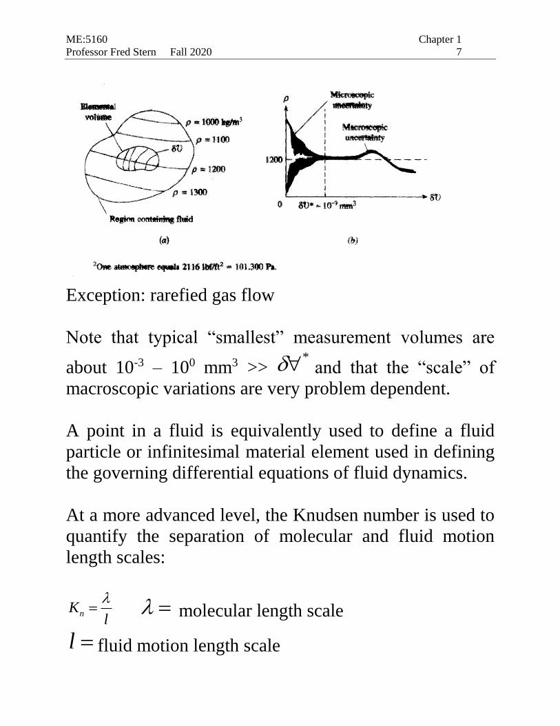
Consider definition of density of a fluid

V

M

VV

limt,x

*

V* = limiting volume below which molecular variations

may be important and above which macroscopic variations

may be important

V* 10-9 mm3 for all liquids and for gases at atmospheric

pressure

10-9 mm3 air (at standard conditions, 20C and 1 atm)

contains 3x107 molecules such that M/V = constant =

x = position vector x y z i j k

t = time

M=mass

ME:5160 Chapter 1


Exception: rarefied gas flow

Note that typical “smallest” measurement volumes are

about 10-3 – 100 mm3 >> * and that the “scale” of

macroscopic variations are very problem dependent.

A point in a fluid is equivalently used to define a fluid

particle or infinitesimal material element used in defining

the governing differential equations of fluid dynamics.

At a more advanced level, the Knudsen number is used to

quantify the separation of molecular and fluid motion

length scales:

nKl

molecular length scale

l fluid motion length scale

ME:5160 Chapter 1


Molecular scales:

Air atmosphere conditions: 86 10 m = mean free path

tλ =10-10 s = time between collisions

Smallest fluid motion scales:

ℓ = 0.1 mm = 10-4 m

Umax ~ 100 m/s incompressible flow 0.3aM

tℓ = 10-6 s

Thus Kn~10-3 << 1, and ℓ scales larger than 3 order of

magnitude scales.

An intermediate scale is used to define a fluid particle

λ << ℓ* << ℓ

And continuum fluid properties are an average over

mmmlmml 63*393** 101010

Previously given smallest fluid motion scales are rough

estimates for incompressible flow. Estimates are VERY

conservative for laminar flow since for laminar flow, l is

usually taken as smallest characteristic length of the flow

domain and Umax can not exceed Re restriction imposed by

transition from laminar to turbulent flow.

For turbulent flow, the smallest fluid motion scales are

estimated by the Kolmogorov scales, which define the

ME:5160 Chapter 1


length, velocity, and time scales at which viscous

dissipation takes place i.e. at which turbulent kinetic

energy is destroyed.

1 4

3 1 2

1 4

u

= kinematic viscosity; =dissipation rate

0

3

00

2

0 // luu is determined by largest scales but occurs at smallest

scales and is independent on v.

Kolmogorov scales can also be written:

4/3

0 Re l Ll 0

4/1

0 Re uu

ULlu 00

0Re

1 2

0 Re

Which even for large Re of interest

*l

For example:

100 watt mixer in 1 kg water: 2 3100 100watt kg m s

6 210 m s for water *210 lmm

ME:5160 Chapter 1


The smallest fluid motion scales for ship and airplane:

U(m/s) L(m) v (m2/s) Re (m)

u

(m/s)

(s)

Ship

(Container: ALIANCA MAUA)

11.8 ( 23.3

knots)

272 9.76E-7 3.3E09 2E-5 0.05 4E-4

Airplane

(Airbus A300)

216.8

(Ma=0.64)

56.2 3.7E-5

(z=10Km)

0.3E09 2.3E-5 1.64 1.4E-

5

Fluid Properties:

(1) Kinematic: linear (V) angular (ω/2) velocity, rate of

strain (εij), vorticity (ω), and acceleration (a).

(2) Transport: viscosity (μ), thermal conductivity (k),

and mass diffusivity (D).

(3) Thermodynamic: pressure (p), density (ρ),

temperature (T), internal energy (û), enthalpy (h

= û + p/ρ), entropy (s), specific heat (Cv, Cp, γ = Cp/

Cv, etc).

(4) Miscellaneous: surface tension (σ), vapor pressure

(pv), etc.

http://www.containership-info.com/vessel_9283239.html

ME:5160 Chapter 1


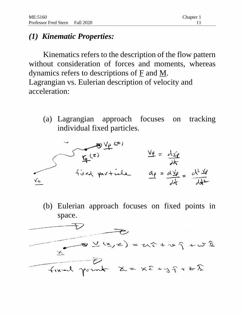
(1) Kinematic Properties:

Kinematics refers to the description of the flow pattern

without consideration of forces and moments, whereas

dynamics refers to descriptions of F and M.

Lagrangian vs. Eulerian description of velocity and

acceleration:

(a) Lagrangian approach focuses on tracking

individual fixed particles.

(b) Eulerian approach focuses on fixed points in

space.

ME:5160 Chapter 1


(u,v,w) = V(x,t) are velocity components in (x,y,z)

directions.

𝑑𝑉(𝑥, 𝑡) =𝜕𝑉

𝜕𝑡𝑑𝑡 +

𝜕𝑉

𝜕𝑥𝑖𝑑𝑥𝑖

However, dxi and dt are not independent since deriviative

is assumed to follow a fluid particle i.e.

𝑑𝑥𝑖 = 𝑢𝑖𝑑𝑡

𝑑𝑉(𝑥, 𝑡)

𝑑𝑡=

𝜕𝑉

𝜕𝑡+

𝜕𝑉

𝜕𝑥𝑖𝑢𝑖

In fluid mechanics special notation is used to define

substantial/material derivative, which follows a fluid

particle:

wz

Vv

y

Vu

x

V

t

V

Dt

VD

VVt

V

Dt

VD)(

, k

zj

yi

xgradient

V

tDt

D = substantial/material derivative = derivative

following motion of particle

Dt

VD = Lagrangian time rate of change of velocity

VVt

V

= local & convective acceleration in terms of

Eulerian derivatives

ME:5160 Chapter 1


𝑎 = 𝑎𝑥𝑖 + 𝑎𝑦𝑗 + 𝑎𝑧𝑘

𝑎𝑥 =𝜕𝑢

𝜕𝑡+ 𝑢

𝜕𝑢

𝜕𝑥+ 𝑣

𝜕𝑢

𝜕𝑦+ 𝑤

𝜕𝑢

𝜕𝑧

𝑎𝑦 =𝜕𝑣

𝜕𝑡+ 𝑢

𝜕𝑣

𝜕𝑥+ 𝑣

𝜕𝑣

𝜕𝑦+ 𝑤

𝜕𝑣

𝜕𝑧

𝑎𝑧 =𝜕𝑤

𝜕𝑡+ 𝑢

𝜕𝑤

𝜕𝑥+ 𝑣

𝜕𝑤

𝜕𝑦+ 𝑤

𝜕𝑤

𝜕𝑧

The Eulerian approach is more convenient since we are

seldom interested in simultaneous time history of

individual fluid particles, but rather time history of fluid

motion (and F, M) in fixed regions in space (control

volumes). However, three fundamental laws of fluid

mechanics (i.e. conservation of mass, momentum, and

energy) are formulated for systems (i.e. particles) and not

control volumes (i.e. regions) and therefore must be

converted from system to CV: Reynolds Transport

Theorem.

V(x,t) is a vector field. Vector operators divergence and

curl lead to other kinematics properties:

z

w

y

v

x

uVdivergenceV

ME:5160 Chapter 1


Dt

D

Dt

D

dd

dddM

particlefluidofvolumeM

11

0

)(

(1)

Continuty: Dt

DVV

Dt

D

10

(2)

(1) and (2): Dt

DV

Dt

D

11

rate of change per unit = - rate of change ρ per unit ρ

For incompressible fluids, ρ = constant

0 V i.e. fluid particles have constant , but not

necessarily shape

ME:5160 Chapter 1


kjiVcurlV zyxˆˆˆ

= vorticity = 2 * angular velocity of fluid particle

ˆˆ ˆi j k

x y z

u v w

ˆˆ ˆw v w u v ui j k

y z x z x y

For irrotational flow 0V

i.e. kz

jy

ix

kwjviuV ˆˆˆˆˆˆ

and for ρ = constant,

0. 2 V Potential Flow Theory

ME:5160 Chapter 1


Other useful kinematic properties include volume and mass

flow-rate (Q,m

), average velocity (V ), and circulation (Γ)

dAnVQ

A

where Q = volume of fluid per unit time

through A ( flux of Vn through A

bounded by S:”flux” generally used to

mean surface integral of variable)

A

dAnVm where m

= mass of fluid per unit time

through A

V = Q/A where V = average velocity through A

A

dAA where A = surface area

ME:5160 Chapter 1


AS

dAVdsV (Stokes theorem - relates line

and area integrals)

line integral for tangential

velocity component = A

dAn

= flux (surface integral) of

normal vorticity

component

Kutta-Joukowski Theorem: lift (L) per unit span for an

aribitrary 2D cylinder in uniform stream U with density ρ

is L = ρUΓ, with direction of L perpendicular to U.

ME:5160 Chapter 1


(2) Transport Properties

There is a close analogy between momentum, heat, and

mass transport; therefore, coefficient of viscosity (μ),

thermal conductivity (k), and mass diffusivity (D) are

referred to as transport properties.

Heat Flux:

Fourier’s Law: q k T 2

J

m s

(rate of heat flux is proportional to the temperature gradient

per unit area; flux is from higher to lower T)

W

kmK

= f(x,y,z) solid

= constant liquid {isotropic}

ME:5160 Chapter 1


Mass Flux:

Fick’s Law: CDq 2

kg

m s

(rate of mass flux is proportional to concentration (C)

gradient per unit area; flux is from higher to lower C)

D

2m

s

Momentum Flux:

Newtonian Fluid: dy

du 2

N

m

1D flow

(rate of momentum flux/shear stress is proportional to the

velocity gradient per unit area, which tends to smooth out

the velocity profile)

ms

kg

m

Ns2

For 3D flow, the shear/rate of strain relationship is more

complex, as will be shown later in the derivation of the

momentum equation.

Vx

u

x

up ij

i

j

j

i

ijij

Where , ,iu u v w , , ,ix x y z

ME:5160 Chapter 1


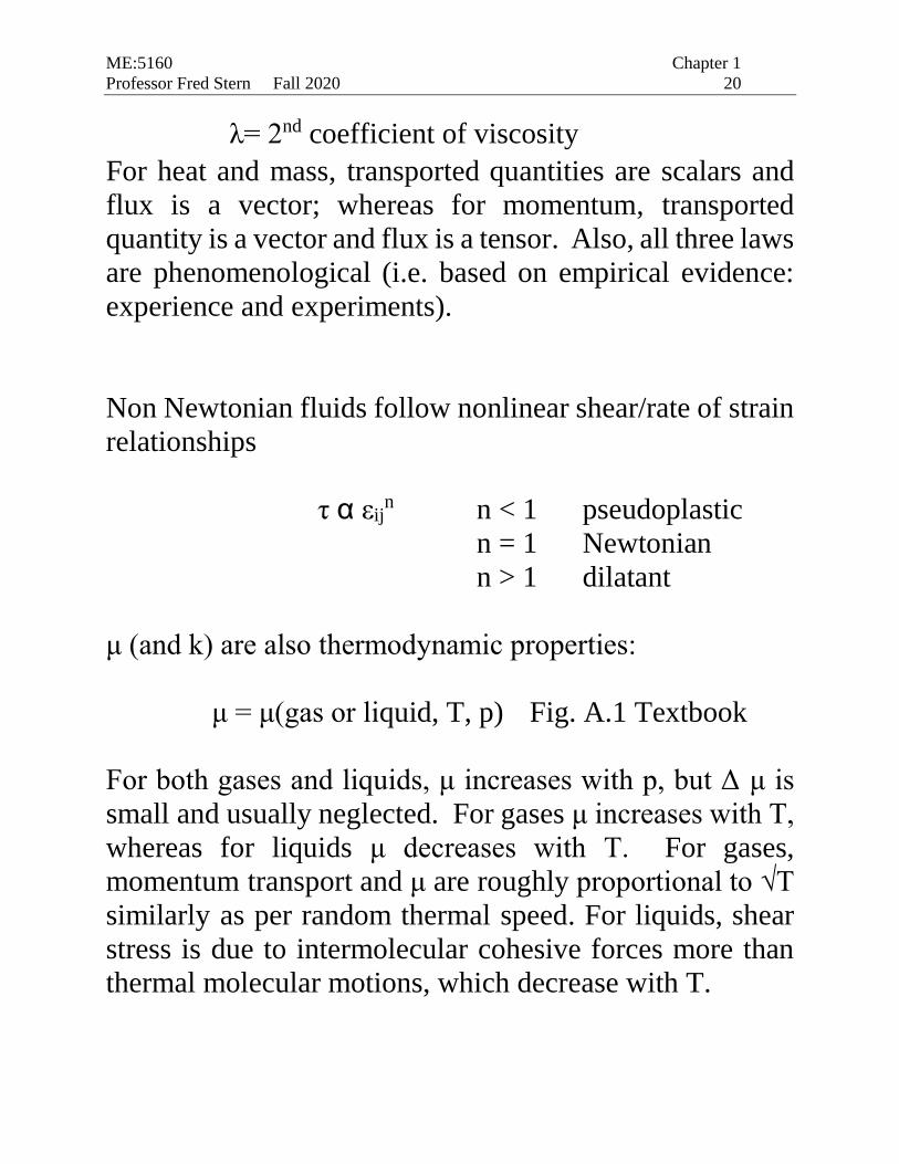
λ= 2nd coefficient of viscosity

For heat and mass, transported quantities are scalars and

flux is a vector; whereas for momentum, transported

quantity is a vector and flux is a tensor. Also, all three laws

are phenomenological (i.e. based on empirical evidence:

experience and experiments).

Non Newtonian fluids follow nonlinear shear/rate of strain

relationships

τ α εijn n < 1 pseudoplastic

n = 1 Newtonian

n > 1 dilatant

μ (and k) are also thermodynamic properties:

μ = μ(gas or liquid, T, p) Fig. A.1 Textbook

For both gases and liquids, μ increases with p, but Δ μ is

small and usually neglected. For gases μ increases with T,

whereas for liquids μ decreases with T. For gases,

momentum transport and μ are roughly proportional to √T

similarly as per random thermal speed. For liquids, shear

stress is due to intermolecular cohesive forces more than

thermal molecular motions, which decrease with T.

ME:5160 Chapter 1


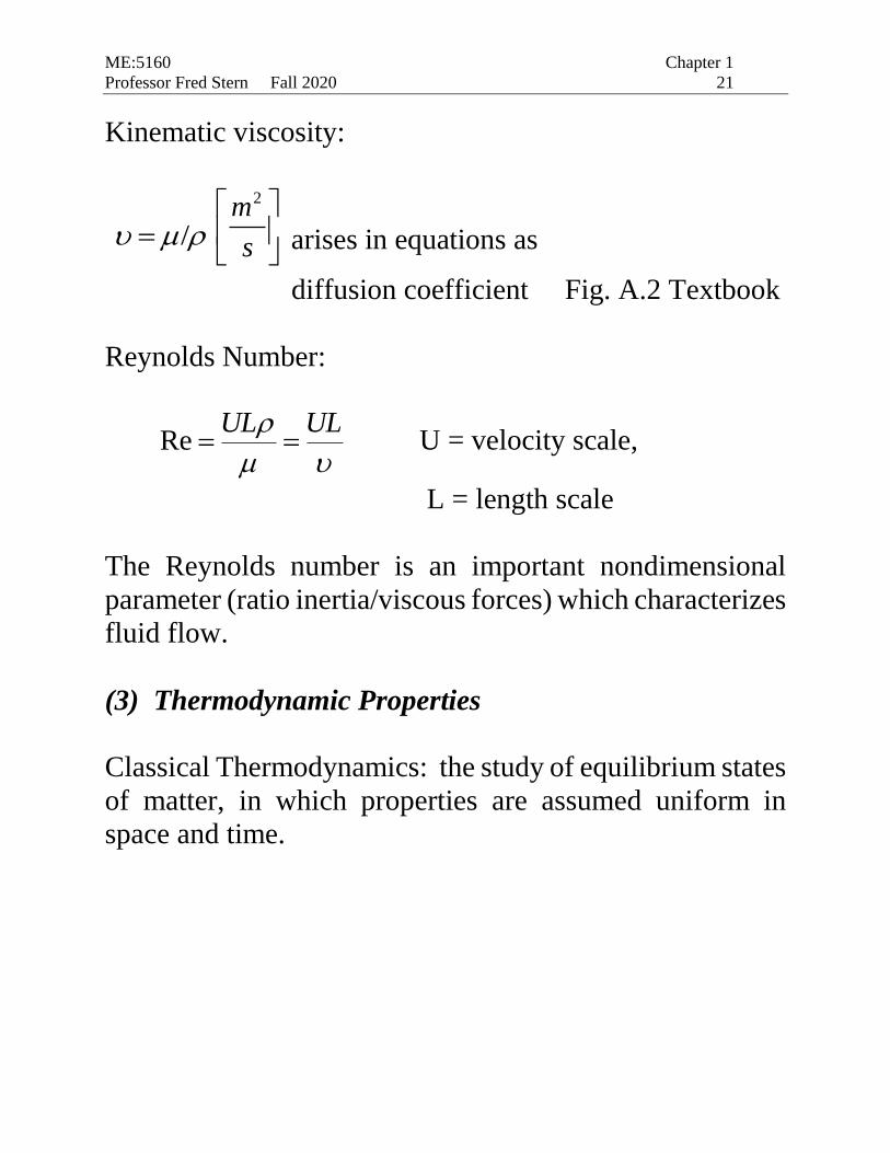
Kinematic viscosity:

/

2m

s

arises in equations as

diffusion coefficient Fig. A.2 Textbook

Reynolds Number:

ULULRe U = velocity scale,

L = length scale

The Reynolds number is an important nondimensional

parameter (ratio inertia/viscous forces) which characterizes

fluid flow.

(3) Thermodynamic Properties

Classical Thermodynamics: the study of equilibrium states

of matter, in which properties are assumed uniform in

space and time.

ME:5160 Chapter 1


Thermodynamic system = fixed mass separated from

surroundings by boundary through which heat and work

are exchanged (but not mass). Properties are state

functions (i.e. depend on current state only and not path),

whereas heat transfer and work are path functions.

A classical thermodynamic system is assumed static,

whereas fluids are often in motion; however, if the

relaxation time (time it takes material to adjust to a new

state) is small compared to the time scale of fluid motion,

an assumption is made that thermodynamic properties are

point functions and that laws and state relations of static

equilibrium thermodynamics are valid. In gases and

liquids at normal pressure, relaxation time is very small;

hence, only a few molecular collisions are needed for

adjustment. Exceptions are rarefied gases, chemically

reacting flows, sudden changes such as shock waves, etc.

For single-phase pure substances, only two properties are

independent and all others follow through equations of

state, which are determined experimentally or

theoretically. Some mixtures, such as air, can also be

considered a pure substance, whereas others such as salt

water cannot and require additional numbers of

independent properties, e.g., sea water requires three

(salinity, T and p)

ME:5160 Chapter 1


Pressure p [N/m2]

Temperature T [K]

Density ρ [kg/m3]

Internal Energy û [Nm/kg] = [J/kg]

Enthalpy h = û + p/ ρ [Nm/kg] = [J/kg]

Entropy s [J/kg K]

ρ = ρ(p,T) û = û(p,T) h = h(p,T) s = s(p,T)

Specific weight γ = ρg [N/m3]

ρair = 1.205 kg/m3 γair = 11.8 N/m3

ρwater = 1000 kg/m3 γwater = 9790 N/m3

ρmercury = 13580 kg/m3 γmercury = 132,948 N/m3

𝑆𝐺𝑔𝑎𝑠 =𝜌𝑔𝑎𝑠

𝜌𝑎𝑖𝑟 (20°𝐶)=

𝜌𝑔𝑎𝑠

1.205 𝑘𝑔/𝑚3 SGair = 1; SGHe = 0.138

3

(4 )1000o

liquid liquid

liquid

water C

SGkg m

SGwater = 1; SGHg = 13.6

ME:5160 Chapter 1


Total stored energy per unit mass (e):

e = û + 1/2V2 + gz

û = energy due to molecular activity and bonding

forces (internal energy)

1/2V2 = work required to change speed of mass from

0 to V per unit mass (kinematic energy)

gz = work required to move mass from 0 to

ˆˆ ˆr xi yj zk against ˆg gk per unit mass

( mrgm / ) (potential energy)

(4) Miscellaneous Properties

Surface Tension:

Two non-mixing liquids or liquids and gases form an

interface across which there is a discontinuity in

density. The interface behaves like a stretched

membrane under tension. The tension originates due

to strong intermolecular cohesive forces in the liquid

that are unbalanced at the interface due to loss of

neighbors, i.e., liquid molecules near the interface pull

the molecules on the interface inward; resulting in

contraction of the interface called surface tension per

unit length.

σ = coefficient of surface tension N/m

ME:5160 Chapter 1


Line force = Fσ = σL where L = length of cut

through interface

σ =f (two fluids, T)

Effects of surface tension (γf not considered):

(1) Pressure jump across curved interfaces

(a) Cylindrical interface

Force Balance:

2σL = 2(pi-po)RL

Δp = σ/R

pi > po , i.e. pressure is larger on concave vs.

convex side of interface

Fluid 1

L Fσ

Fluid 2 Direction of Fσ is normal to

cut

ME:5160 Chapter 1


(b) Spherical interface (droplet)

2πRσ = πR2 Δp Δp = 2σ/R

(c) Bubble

2πRσ+2πRσ = πR2 Δp Δp = 4σ/R

(d) General interface

Δp = σ(R1-1 + R2

-1)

R1,2 = principle radii of curvature

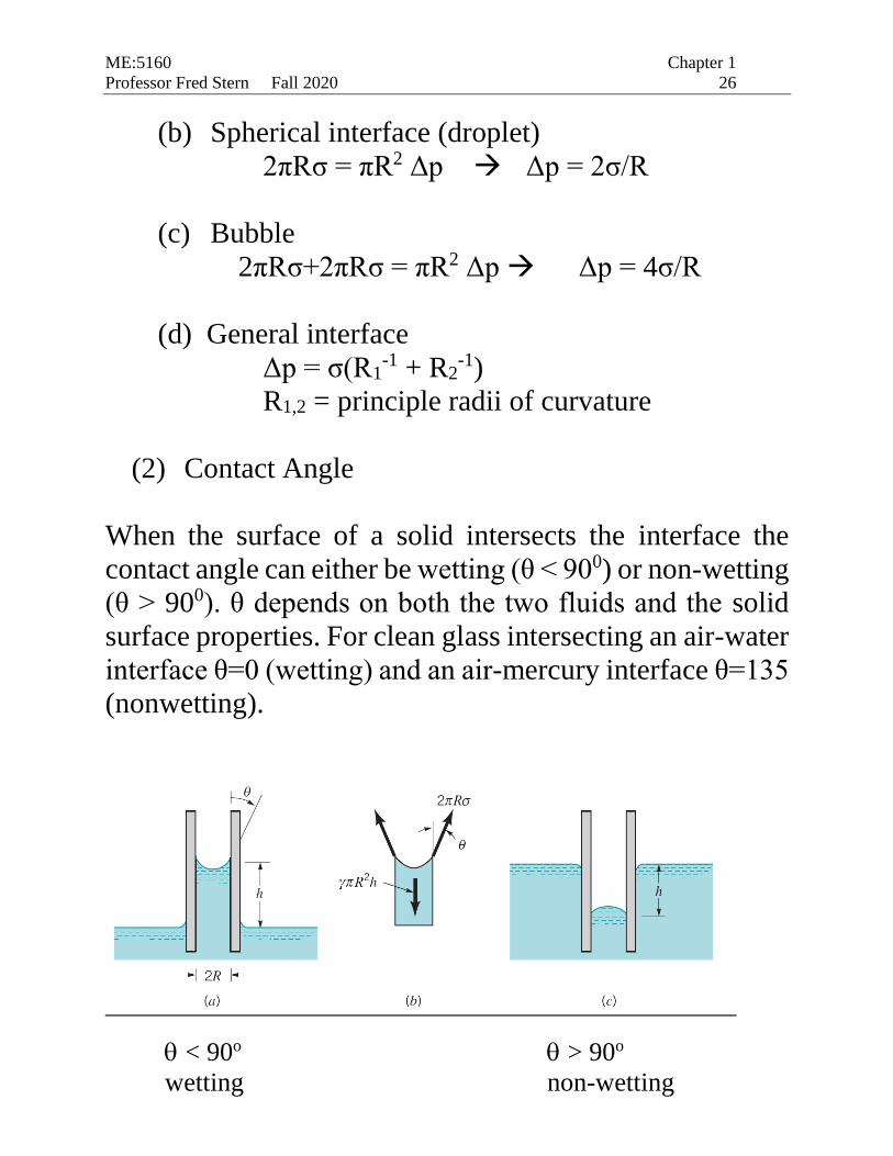
(2) Contact Angle

When the surface of a solid intersects the interface the

contact angle can either be wetting (θ < 900) or non-wetting

(θ > 900). θ depends on both the two fluids and the solid

surface properties. For clean glass intersecting an air-water

interface θ=0 (wetting) and an air-mercury interface θ=135

(nonwetting).

< 90o

wetting

> 90o

non-wetting

ME:5160 Chapter 1


Capillary tube

Surface Tension Force = Weight of fluid

2πRσ cos θ = ρghπR2

R

h

cos2 h α R-1 (i.e. larger h for smaller R)

h > 0 = wetting, h < 0 = non-wetting

patm

p(z)

Jump across

boundary

due to σ

h

patm

patm patm

Pressure jump

due to σ

p=patm+γh p(z)

p=patm – γh

p > concave, i.e. air side

Non-wetting

drives liquid

down tube

p > concave, i.e. water side

ME:5160 Chapter 1


(b) Parallel plates

For two parallel plates 2R apart with depth b:

Surface Tension Force = Weight of fluid

2bσ cos θ = ρgh2Rb Rh

cos

(c) Pressure jump

wetting-non

wetting

h

h

ppppzczpdz

dpatmhzhzatatm

For general interface:

h>0 (wetting):

1 1

1 2( ) 0 water airp R R h p p concave

shape

h<0 (non-wetting): 1 1

1 2( ) 0 water airp R R h p p convex

shape

ME:5160 Chapter 1


(3) Transformation liquid jet into droplets

(4) Binding of wetted granular material such as sand

(5) Capillary waves

Similar to stretched membrane (string) waves, surface

tension acts as restoring force resulting in interfacial waves

called capillary waves.

Cavitation:

When the pressure in a liquid falls below the vapor

pressure, it will evaporate (i.e. become a gas). If due to

temperature changes alone, the process is called boiling,

whereas if due to liquid velocity, the process is called

cavitation.

22/1 U

ppCa va

Ca = Cavitation #

pv = vapor pressure

pa = ambient pressure

U = characteristic velocity

If the local pressure coefficient Cp ( 21/ 2

ap pCp

U

) falls

below the cavitation number Ca, the liquid will cavitate.

ME:5160 Chapter 1


Ca = f (liquid/properties, T)

Effects of cavitation:

(1) erosion

(2) vibration

(3) noise

ME:5160 Chapter 1


Flow Classification:

(1) Spatial dimensions: 1D, 2D, 3D

(2) Steady or unsteady: 0

t or 0

t

(3) Compressible (ρ constant) or incompressible (ρ =

constant)

(4) Inviscid or Viscous: μ = 0 or μ 0.

(5) Rotational or Irrotational: ω 0 or ω = 0.

(6) Inviscid/Irrotational: potential flow

(7) Viscous, laminar or turbulent: Retrans

(8) Viscous, low Re: Stokes flow

(9) Viscous, high Re external flow: boundary layer

(10) Etc.

Depending on flow classification, different approximations

can be made to exact governing differential equations

resulting in different forms of approximate equations and

analysis techniques.

ME:5160 Chapter 1


Flow Analysis Techniques:

“Reality”

Fluids Eng. Systems Components Idealized

EFD

Mathematical Physics Problem Formulation

AFD

CFD

Class Notes Fall 2020 - user.engineering.uiowa.edu

Documents

Transcript of Class Notes Fall 2020 - user.engineering.uiowa.edu