Cladogram Building - 1
33
Cladogram Cladogram Building - 1 Building - 1 How complex is this problem anyway ? # taxa # cladograms 3 3 4 15 5 105 6 945 10 34.459.425 20 > 8.200 E18 NP-complete: Time needed to find solution in-creases exponentially with size of problem -> t = c n
-
Upload
basia-santiago -
Category
Documents
-
view
62 -
download
5
description
Cladogram Building - 1. How complex is this problem anyway ?. NP-complete: Time needed to find solution in-creases exponentially with size of problem -> t = c n. Computational Complexity. How do we proceed ? What about the quality of the solution ? Optimality criterion - PowerPoint PPT Presentation
Transcript of Cladogram Building - 1
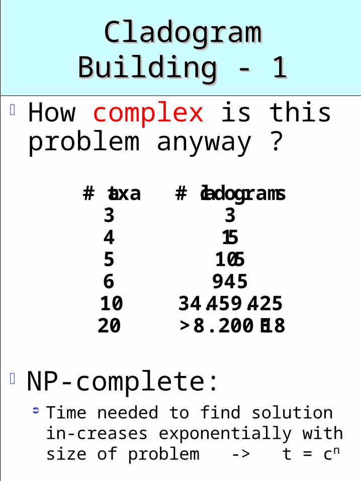
Cladogram Building Cladogram Building - 1- 1
How complex is this problem anyway ?
# taxa # cladograms3 34 155 1056 94510 34.459.42520 > 8.200 E18
NP-complete: Time needed to find solution in-
creases exponentially with size of problem -> t = cn
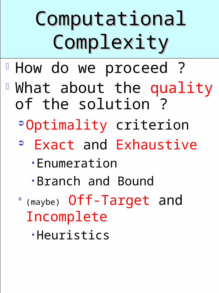
Computational Computational ComplexityComplexity
How do we proceed ?What about the quality of the solution ?Optimality criterion Exact and Exhaustive
•Enumeration•Branch and Bound
(maybe) Off-Target and Incomplete•Heuristics
Optimality - 1Optimality - 1
Parsimony analysis:comprises a group of related methods, united by the goal of optimizing some evolutionary significant quantity but differing in their underlying evolutionary assumptions.
Optimality - 2Optimality - 2
How good is the solution : What is its score [relative to
alternatives]?. Relation of score to
evolutionary assumptions Fitch and Wagner Parsimony Dollo Parsimony Camin-Sokal Parsimony Generalized Parsimony Constrained Parsimony
• Group / Component Compatibility
• Character Compatibility
Exact and Exact and ExhaustiveExhaustive
Enumeration is computationally unfeasible if # taxa is over, say, 10.
Branch and Bound is computationally feasible for over 20 taxa (50 may even work).
(maybe) Off-Target (maybe) Off-Target andand IncompleteIncomplete
HeuristicsStep-wise AdditionStar DecompositionBranch Swapping

Step-wise Addition Step-wise Addition - 1- 1
D
A
E C
B
E
A
D C
B
A
B
C
BA
CDBA
CDB
A C
D
A
D
B E
C
DE
A
B C B E
C
DA
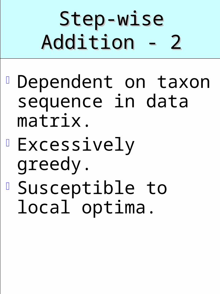
Step-wise Addition Step-wise Addition - 2- 2
Dependent on taxon sequence in data matrix.
Excessively greedy.Susceptible to local optima.
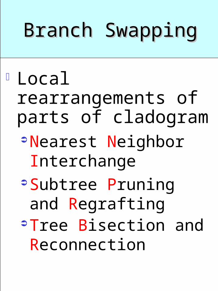
Branch SwappingBranch Swapping
Local rearrangements of parts of cladogramNearest Neighbor Interchange
Subtree Pruning and Regrafting
Tree Bisection and Reconnection
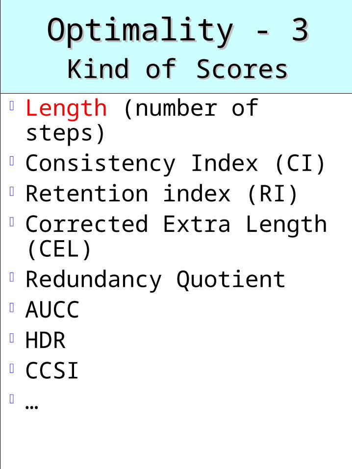
Optimality - 3 Optimality - 3 Kind Kind
ofof ScoresScores Length (number of steps) Consistency Index (CI) Retention index (RI) Corrected Extra Length
(CEL) Redundancy Quotient AUCC HDR CCSI …
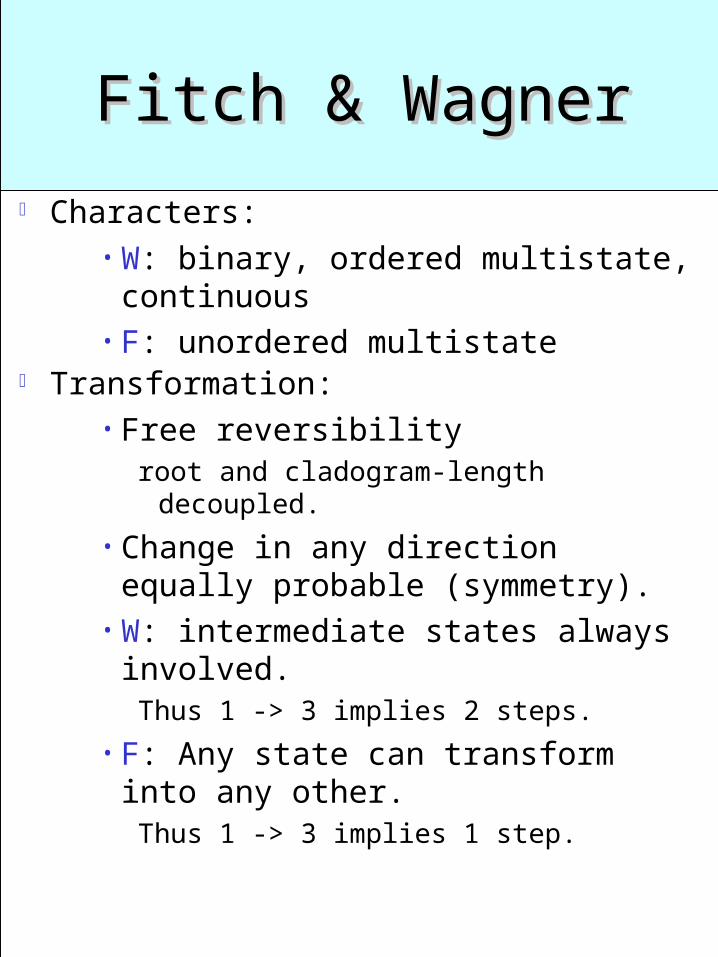
Fitch & WagnerFitch & Wagner
Characters:• W: binary, ordered multistate,
continuous• F: unordered multistate
Transformation:• Free reversibility
root and cladogram-length decoupled.
• Change in any direction equally probable (symmetry).
• W: intermediate states always involved.Thus 1 -> 3 implies 2 steps.
• F: Any state can transform into any other.Thus 1 -> 3 implies 1 step.

Wagner:Wagner:Cladogram length - 1Cladogram length - 1
B
C
A D
E
B C
A
D E0B C
2 1 3
0A
D E
0,2 1,3
1,2
? ?
?
0 2 1 3
0
0B C
2 1 3
0A
D E
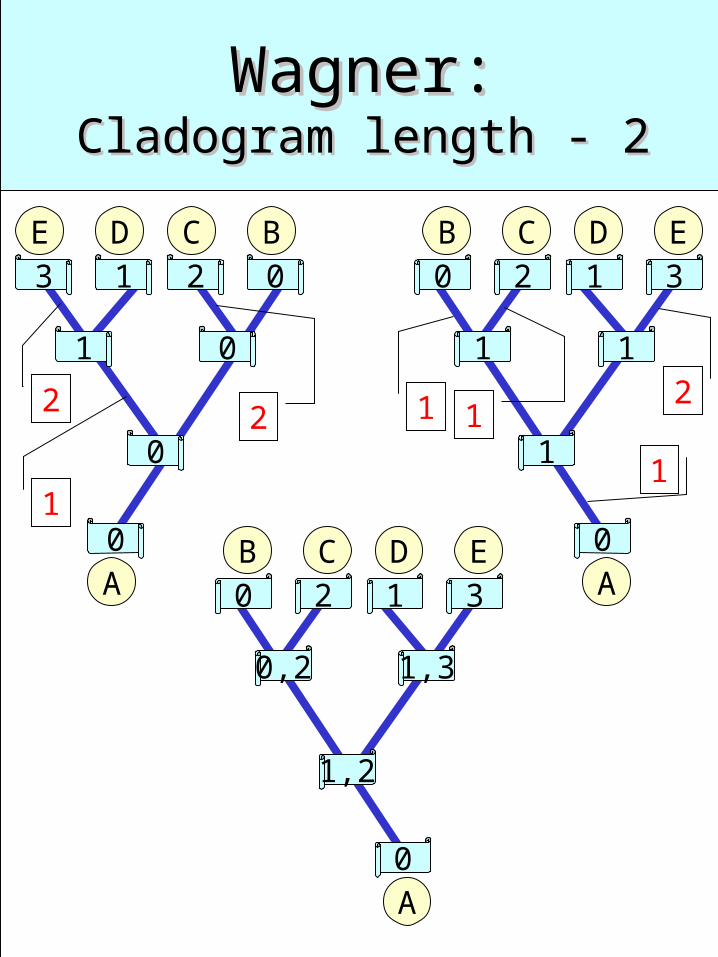
Wagner:Wagner:Cladogram length - 2Cladogram length - 2
0B C
2 1 3
0A
D E
0,2 1,3
1,2
1
1
0BC
213
0A
DE
1 0
0
1
2
1
1 1
1
22

Fitch:Fitch:Cladogram lengthCladogram length
A
E
D B
C
0 2 0 3
2
B C
A
D E
0,2
0
0,3
0 2 0 3
2
B C
A
D E
0
0
0
1
1
1

A B
C
D
E
Dollo:Dollo:Multiple origins not allowedMultiple origins not allowed
0 1
0
1
0
A B
C
D
E
0 1
0
1
0
0
0
0
1
1
1

Generalized Generalized ParsimonyParsimony
1 2 31 2
1
a b c d
abcd
12 13 2 1
Wagner
1 1 11 1
1
a b c d
abcd
11 11 1 1
Fitch
M 2M 3MM 2M
M
a b c d
abcd
12 13 2 1
Dollo
5 1 55 1
5
A C G T
ACGT
51 55 1 5
T-sition/T-version
1Gain vs
Loss
0 1
01
1
Models Models of Evolutionary Changeof Evolutionary Change
Molecular DataMaximum Likelihood: “Given the phylogeny, what is the probability to find the data as I did ?”
Substitution TypesSubstitution Probabilities
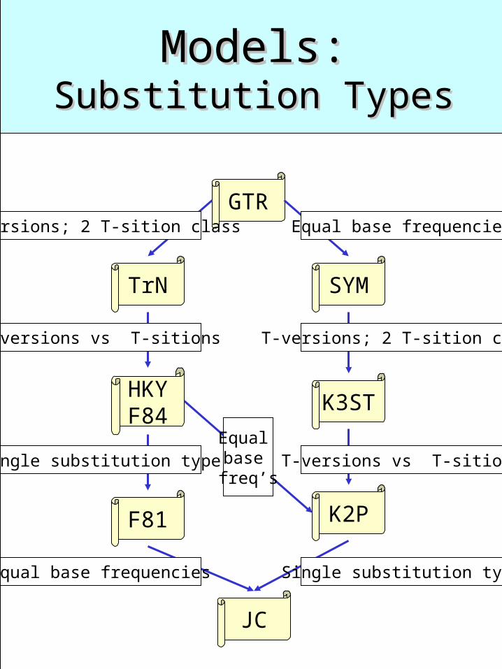
Models:Models:Substitution TypesSubstitution Types
GTR
TrN SYM
HKYF84
K3ST
F81 K2P
JC
T-versions; 2 T-sition class
T-versions vs T-sitions
Single substitution type
Single substitution typeEqual base frequencies
Equal base frequencies
T-versions; 2 T-sition class
T-versions vs T-sitionsEqual base freq’s

Substitution Types: Substitution Types: What do they all mean ?What do they all mean ?
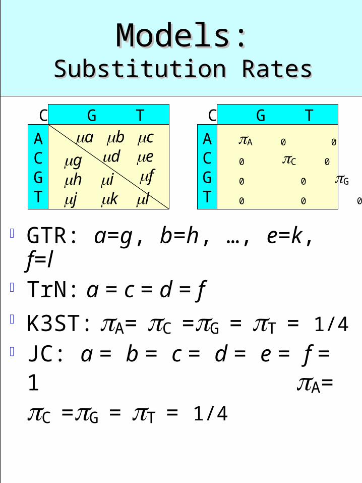
GTR, e.g., stands for Generalized Time Reversible, meaning that the overall rate of change from base i to base j in a given length of time is the same as the rate of change from base j to base i.
Each type corresponds to a table of substitution rates for all pairs of the nucleotides A, C, G, and T
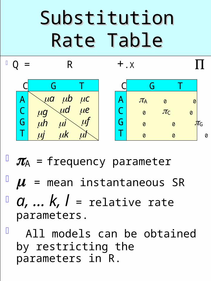
Substitution Rate Substitution Rate TableTable
Q = R +.X
A0 0 0
0C0 0
0 0G 0
0 0 0T
ACGT
A C G T a b c
def
A C G T
ACGT
gh ij k l
A = frequency parameter
= mean instantaneous SR
a, … k, l = relative rate parameters.
All models can be obtained by restricting the parameters in R.
Models:Models:Substitution RatesSubstitution Rates
GTR: a=g, b=h, …, e=k, f=l TrN: a = c = d = f K3ST: A= C =G = T = 1/4 JC: a = b = c = d = e = f =
1 A= C =G
= T = 1/4
A0 0 0
0C0 0
0 0G 0
0 0 0T
ACGT
A C G T a b c
def
A C G T
ACGT
gh ij k l
Models:Models:Substitution ProbabilitiesSubstitution Probabilities
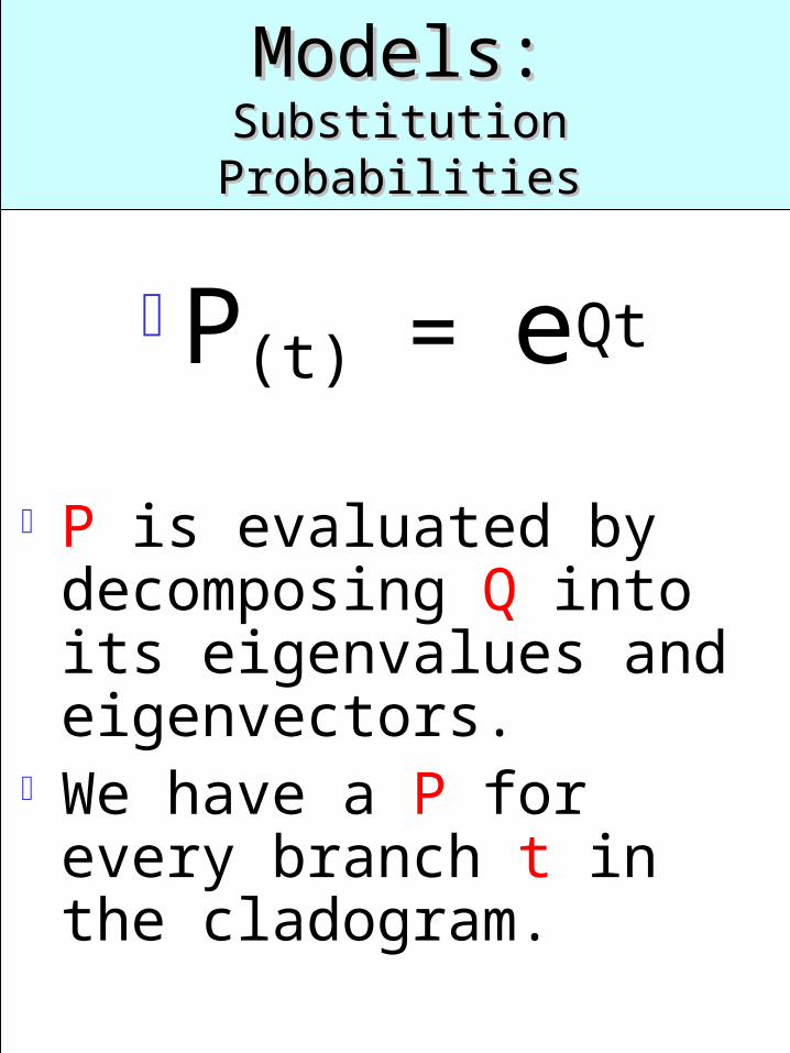
P(t) = eQt
P is evaluated by decomposing Q into its eigenvalues and eigenvectors.
We have a P for every branch t in the cladogram.
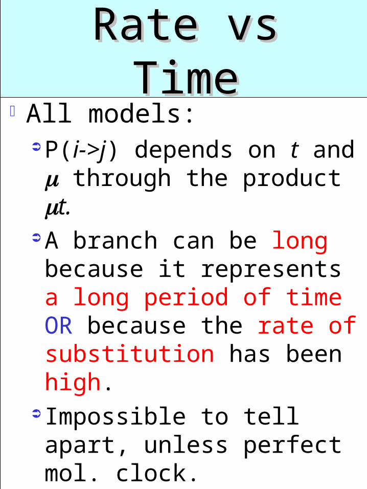
Rate vs TimeRate vs TimeAll models:
P(i->j) depends on t and through the product t.
A branch can be long because it represents a long period of time OR because the rate of substitution has been high.
Impossible to tell apart, unless perfect mol. clock.
Rate + Time =Rate + Time =
Branch LengthBranch Length
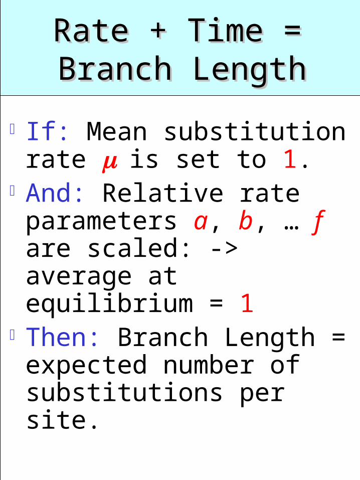
If: Mean substitution rate is set to 1.
And: Relative rate parameters a, b, … f are scaled: -> average at equilibrium = 1
Then: Branch Length = expected number of substitutions per site.
Recap.Recap.
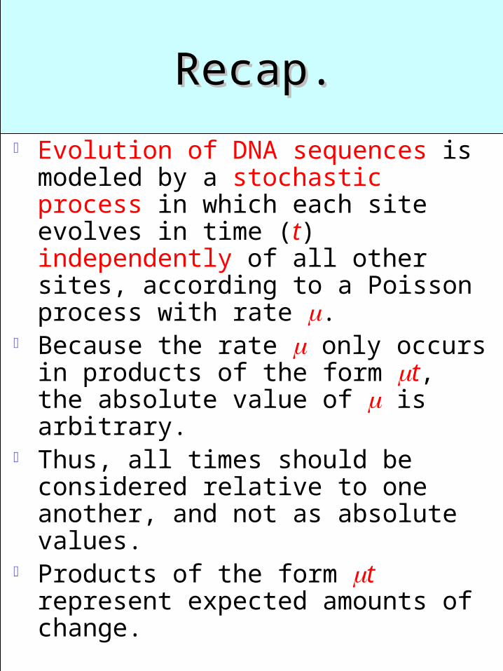
Evolution of DNA sequences is modeled by a stochastic process in which each site evolves in time (t) independently of all other sites, according to a Poisson process with rate .
Because the rate only occurs in products of the form t, the absolute value of is arbitrary.
Thus, all times should be considered relative to one another, and not as absolute values.
Products of the form t represent expected amounts of change.
Likelihood of a Likelihood of a Cladogram - 1Cladogram - 1
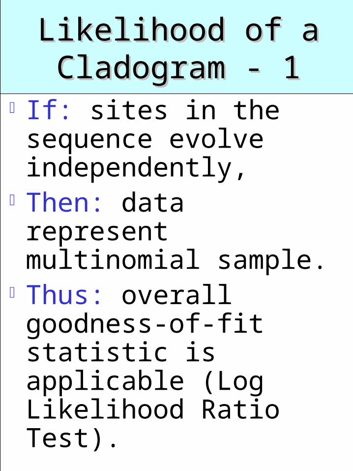
If: sites in the sequence evolve independently,
Then: data represent multinomial sample.
Thus: overall goodness-of-fit statistic is applicable (Log Likelihood Ratio Test).
Likelihood of a Likelihood of a Cladogram - 2Cladogram - 2
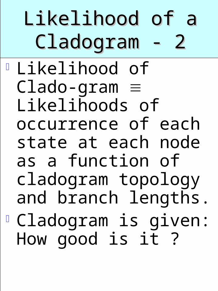
Likelihood of Clado-gram Likelihoods of occurrence of each state at each node as a function of cladogram topology and branch lengths.
Cladogram is given: How good is it ?
Likelihood of a Likelihood of a Cladogram - 3Cladogram - 3
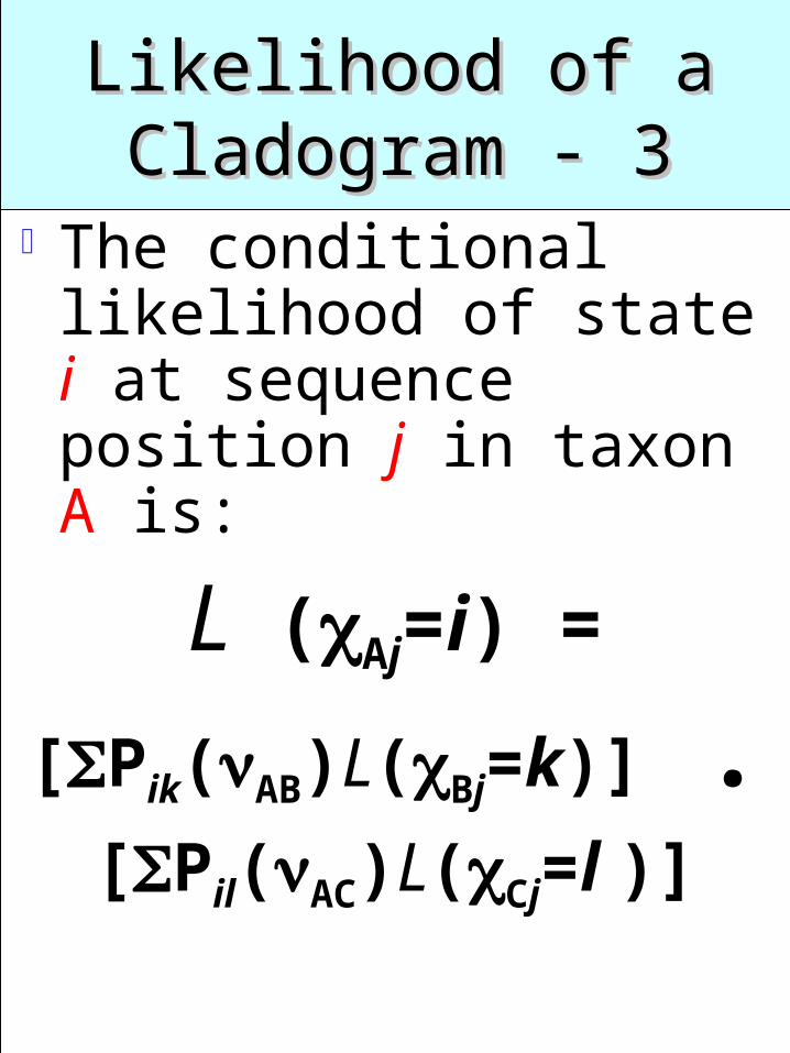
The conditional likelihood of state i at sequence position j in taxon A is:
L (Aj=i) =
[Pik(AB)L(Bj=k)] .
[Pil(AC)L(Cj=l )]
Likelihood of a Likelihood of a Cladogram - 4Cladogram - 4
See figure 10 in SOWH.
Maximum Maximum LikelihoodLikelihood
Pro: Consistency As the number of items of
data (n) increases, the probability that the estimator is far from the true value of the parameter (cladogram structure) decreases to zero.
But: Inferential consistency
depends on the model. Only finite amounts of data
are considered, thus a ‘long-term’ property is not necessary.
Maximum Maximum Likelihood - 2Likelihood - 2
“Anyone who considers this model (Poisson Process Model of DNA substitution) complex should bear in mind that it is the simplest mathematical model of state change with constant probabilities per unit time, and that a particular case (that of a very low rate of change) is used to justify parsimony methods.
The model does not allow for insertions, deletions, and inversions.

When does ML = When does ML = Parsimony ?Parsimony ?
They estimate different parameters, therefore the estimates cannot match exactly.
For cladogram structure alone: If PPM is correct, and we
assume the expected amount of change, t, to be very small, then the probability structures become the same.
For realistic values of t, the two models do not behave identically.
Extensions of MLExtensions of ML
Rate heterogeneity among sites
Other data types (except sequences)gene frequenciesrestriction sites
Pairwise Distance Methods immunological dataDNA-DNA hybridizations