COST-EFFECTIVENESS AND PERFORMANCE OF OVERLAY SYSTEMS IN ILLINOIS

VOLUME 2: GUIDELINES FOR INTERLAYER SYSTEM SELECTION DECISION WHEN USED

IN HMA OVERLAYS

Prepared By Imad L. Al-Qadi

William G. Buttlar Jongeun Baek

University of Illinois at Urbana-Champaign

Research Report ICT-09-045

A report of the findings of

ICT-R58 Cost-Effectiveness and Performance of Overlay Systems in Illinois

Illinois Center for Transportation

May 2009

CIVIL ENGINEERING STUDIES Illinois Center for Transportation Series No. 09-045

UILU-ENG-2009-2016 ISSN: 0197-9191

Technical Report Documentation Page 1. Report No.

FHWA-ICT-09-045

2. Government Accession No. 3. Recipient's Catalog No.

4. Title and Subtitle

Cost-Effectiveness and Performance of Overlay Systems in Illinois Volume 2:Guidelines for Interlayer System Selection Decision When Used in HMA Overlays

5. Report Date

May 2009 6. Performing Organization Code

8. Performing Organization Report N o. 7. Author(s)

Imad L. Al-Qadi, William G. Buttlar, and Jongeun Baek

ICT-009-045 UILU-ENG-2009-2016

9. Performing Organization Name and Address 10. Work Unit ( TRAIS)

Illinois Center for Transportation Department of Civil and Environmental Engineering

11. Contract or Grant No.

ICT-R58

University of Illinois at Urbana-Champaign 205 N. Mathews Ave., MC-250 Urbana, IL 61801

13. Type of Report and Period Covered

Project Report 2005-2008

12. Sponsoring Agency Name and Address

Illinois Department of Transportation Bureau of Materials and Physical Research

126 East Ash Street Springfield, IL 62704-4766

14. Sponsoring Agency Code

15. Supplementary Notes

16. Abstract

In an effort to control reflective cracking in hot-mix asphalt (HMA) overlays placed over Portland Cement Concrete (PCC) pavements, several reflective crack control (RCC) systems, including interlayer systems, have been used. However, the cost-effectiveness of interlayer systems is still in doubt due their performance and additional costs. In this project, a decision making procedure to aid in the selection of cost-effective interlayer systems was developed. As a core step in evaluating the benefit-cost ratio (B/C) of interlayer systems, a user-friendly life-cycle cost analysis (LCCA) program, CIND (Cost-effective INterlayer system Decision program) was developed. Based on sensitivity analysis, a B/C prediction model was proposed, which takes into account a performance benefit ratio (PBR) parameter, a material cost ratio (MCR), and a construction time ratio (CTR). Using the B/C model, a table was developed which allows the user to determine the most cost-effective interlayer system in a rehabilitation project for a given equivalent single-axle load (ESAL) level, representative low temperature (TL), and existing concrete pavement joint spacing (JS). Finally, a decision making tree was constructed to simplify the process of determining the most cost-effective and compatible interlayer system for a given project. Depending on project significance and/or information availability, pavement engineers can select from one of three newly developed B/C evaluation tools (in order of sophistication): application tables, B/C prediction model, and the CIND computer program. Using these tools, it was found that B/C increases as PBR increases or MCR and CTR decrease. In general, System D is cost-effective in a wide range of ESALs and TL values; especially in a cold region with lower traffic volume. The application range is reduced with the increase of JS, however. System E is relatively cost-effective only in warm regions having higher traffic volume.

17. Key Words

18. Distribution Statement

No restrictions. This document is available to the public through the National Technical Information Service, Springfield, Virginia 22161.

19. Security Classif. (of this report)

Unclassified

20. Security Classif. (of this page)

Unclassified

21. No. of Pages

88

22. Price

Form DOT F 1700.7 (8-72) Reproduction of completed page authorized

ii

ACKNOWLEDGMENT AND DISCLAIMER This publication is based on the results of ICT-R58, COST-EFFECTIVENESS AND PERFORMANCE OF OVERLAY SYSTEMS IN ILLINOIS. ICT-R58 was conducted in cooperation with the Illinois Center for Transportation; the Illinois Department of Transportation, Division of Highways; and the Federal Highway Administration of the U.S. Department of Transportation. Members of the Technical Review Panel are the following: Joseph Vespa, IDOT Amy Schutzbach, IDOT David Lippert, IDOT Jim Trepanier, IDOT Aaron Toliver, IDOT Patty Broers, IDOT The contents of this report reflect the view of the authors who are responsible for the facts and the accuracy of the data presented herein. The contents do not necessarily reflect the official views or policies of the Illinois Center for Transportation, the Illinois Department of Transportation, or the Federal Highway Administration. This report does not constitute a standard, specification, or regulation. Trademark or manufacturers’ names appear in this report only because they are considered essential to the object of this document and do not constitute an endorsement of product by the Federal Highway Administration, the Illinois Department of Transportation, or the Illinois Center for Transportation.

iii

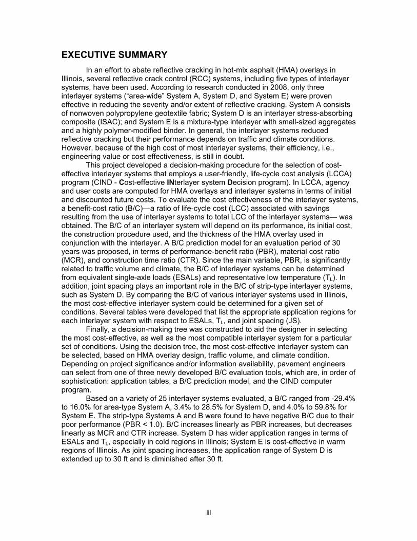
EXECUTIVE SUMMARY In an effort to abate reflective cracking in hot-mix asphalt (HMA) overlays in

Illinois, several reflective crack control (RCC) systems, including five types of interlayer systems, have been used. According to research conducted in 2008, only three interlayer systems (“area-wide” System A, System D, and System E) were proven effective in reducing the severity and/or extent of reflective cracking. System A consists of nonwoven polypropylene geotextile fabric; System D is an interlayer stress-absorbing composite (ISAC); and System E is a mixture-type interlayer with small-sized aggregates and a highly polymer-modified binder. In general, the interlayer systems reduced reflective cracking but their performance depends on traffic and climate conditions. However, because of the high cost of most interlayer systems, their efficiency, i.e., engineering value or cost effectiveness, is still in doubt. This project developed a decision-making procedure for the selection of cost-effective interlayer systems that employs a user-friendly, life-cycle cost analysis (LCCA) program (CIND - Cost-effective INterlayer system Decision program). In LCCA, agency and user costs are computed for HMA overlays and interlayer systems in terms of initial and discounted future costs. To evaluate the cost effectiveness of the interlayer systems, a benefit-cost ratio (B/C)—a ratio of life-cycle cost (LCC) associated with savings resulting from the use of interlayer systems to total LCC of the interlayer systems— was obtained. The B/C of an interlayer system will depend on its performance, its initial cost, the construction procedure used, and the thickness of the HMA overlay used in conjunction with the interlayer. A B/C prediction model for an evaluation period of 30 years was proposed, in terms of performance-benefit ratio (PBR), material cost ratio (MCR), and construction time ratio (CTR). Since the main variable, PBR, is significantly related to traffic volume and climate, the B/C of interlayer systems can be determined from equivalent single-axle loads (ESALs) and representative low temperature (TL). In addition, joint spacing plays an important role in the B/C of strip-type interlayer systems, such as System D. By comparing the B/C of various interlayer systems used in Illinois, the most cost-effective interlayer system could be determined for a given set of conditions. Several tables were developed that list the appropriate application regions for each interlayer system with respect to ESALs, TL, and joint spacing (JS).

Finally, a decision-making tree was constructed to aid the designer in selecting the most cost-effective, as well as the most compatible interlayer system for a particular set of conditions. Using the decision tree, the most cost-effective interlayer system can be selected, based on HMA overlay design, traffic volume, and climate condition. Depending on project significance and/or information availability, pavement engineers can select from one of three newly developed B/C evaluation tools, which are, in order of sophistication: application tables, a B/C prediction model, and the CIND computer program. Based on a variety of 25 interlayer systems evaluated, a B/C ranged from -29.4% to 16.0% for area-type System A, 3.4% to 28.5% for System D, and 4.0% to 59.8% for System E. The strip-type Systems A and B were found to have negative B/C due to their poor performance (PBR < 1.0). B/C increases linearly as PBR increases, but decreases linearly as MCR and CTR increase. System D has wider application ranges in terms of ESALs and TL, especially in cold regions in Illinois; System E is cost-effective in warm regions of Illinois. As joint spacing increases, the application range of System D is extended up to 30 ft and is diminished after 30 ft.

iv

TABLE OF CONTENTS Acknowledgment and Disclaimer ...................................................................................... ii 

Executive Summary .......................................................................................................... iii 

Table of Contents ............................................................................................................. iv 

1. Introduction ................................................................................................................... 1 

1.1 BACKGROUND ....................................................................................................... 1 

1.2 REFLECTIVE CRACK CONTROL IN ILLINOIS ...................................................... 1 

1.3 LIFE-CYCLE COST ANALYSIS .............................................................................. 2 

1.4 DECISION-MAKING PROCEDURE IN PAVEMENT DESIGN ................................ 3 

2. INTERLAYER SYSTEM DECISION PROCEDURE ..................................................... 4 

2.1 GENERAL PROCEDURE ....................................................................................... 4 

2.2 INTERLAYER SYSTEM PERFORMANCE EVALUATION ..................................... 5 

2.3 LIFE-CYCLE COST ANALYSIS FOR HMA OVERLAYS ........................................ 6 

2.3.1 Agency Cost ...................................................................................................... 6 

2.3.2 User Cost .......................................................................................................... 6 

2.3.3 Expenditure Diagram ........................................................................................ 7 

2.3.4 Net Present Value and Equivalent Uniform Annual Cost .................................. 8 

2.4 COST-EFFECTIVE INTERLAYER SYSTEM DECISION PROGRAM (CIND) ........ 9 

2.4.1 Input Module ................................................................................................... 10 

2.4.2 Output Module ................................................................................................ 14 

3. EVALUATION OF COST EFFECTIVENESS OF INTERLAYER SYSTEMS .............. 15 

3.1 COST BENEFIT .................................................................................................... 15 

3.1.1 System A (Area) .............................................................................................. 16 

3.1.2 System A (Strip) and System B ...................................................................... 17 

3.1.3 System D ........................................................................................................ 18 

3.1.4 System E ......................................................................................................... 19 

3.2 COST-EFFECTIVENESS EVALUATION OF THE INTERLAYER SYSTEMS ...... 20 

3.2.1 Short-Term Evaluation .................................................................................... 21 

3.2.2 Long-Term Evaluation ..................................................................................... 24 

4. DEVELOPMENT OF A B/C PREDICTION MODEL .................................................... 26 

4.1 B/C VARIABLES .................................................................................................... 26 

4.1.1 Material Cost Ratio ......................................................................................... 27 

4.1.2 Construction Time Ratio ................................................................................. 29 

4.1.3 Typical Values of B/C Variables ...................................................................... 30 

v

4.2 B/C PREDICTION MODEL AND EFFECT OF THE MAIN VARIABLES ............... 30 

4.3 MODEL VALIDATION ........................................................................................... 36 

4.4 APPLICATION RANGE OF INTERLAYER SYSTEMS ......................................... 38 

5. INTERLAYER SYSTEM SELECTION DECISION-MAKING ....................................... 44 

5.1 DECISION TREE FOR INTERLAYER SYSTEM SELECTION ............................. 44 

5.2 DECISION TREE VALIDATION ............................................................................ 47 

6. CONCLUSIONS AND RECOMMENDATIONS ........................................................... 49 

6.1 SUMMARY ............................................................................................................ 49 

6.2 EXPECTED BENEFITS ......................................................................................... 49 

6.3 RECOMMENDATIONS ......................................................................................... 50 

7. REFERENCES ............................................................................................................ 51 

APPENDIX A ................................................................................................................. A-1 

APPENDIX B ................................................................................................................. B-1 

1

1. INTRODUCTION

1.1 BACKGROUND Hot-mix asphalt (HMA) overlays are a pavement rehabilitation commonly used

for the renewal of structurally or functionally deteriorated pavements. The new AASHTO mechanistic–empirical pavement design guide proposes three HMA overlay design approaches, depending on whether the existing pavement type is HMA, fractured concrete, or an intact concrete pavement—including composite pavement (NCHRP, 2003). For each of these, pre-overlay repairs are typically conducted prior in order to enhance the performance of the HMA overlay which follows. For example, cracking and seating, breaking and seating, rubblization, patching, slab jacking, and dowel bar retrofitting can be applied to concrete pavements, while milling, patching, and crack sealing are treatments usually used to repair flexible pavements prior to the placement of an overlay. Several methods are also sometimes used to control reflective cracking, such as the use of a thicker HMA overlay, sawing and sealing of joints in the new overlay, the placement of synthetic fabrics or steel netting below or between paving lifts in the overlay, or the application of a crack relief layer. Among these methods, interlayer systems have generally been found to be among the most cost efficient for controlling reflective cracking. However, interlayer systems can sometimes be costly, depending on the nature of the system used, in terms of both material and construction costs. Thus, cost effectiveness should be considered as part of overlay system design.

1.2 REFLECTIVE CRACK CONTROL IN ILLINOIS HMA overlays are designed based on existing pavement, traffic, and climate

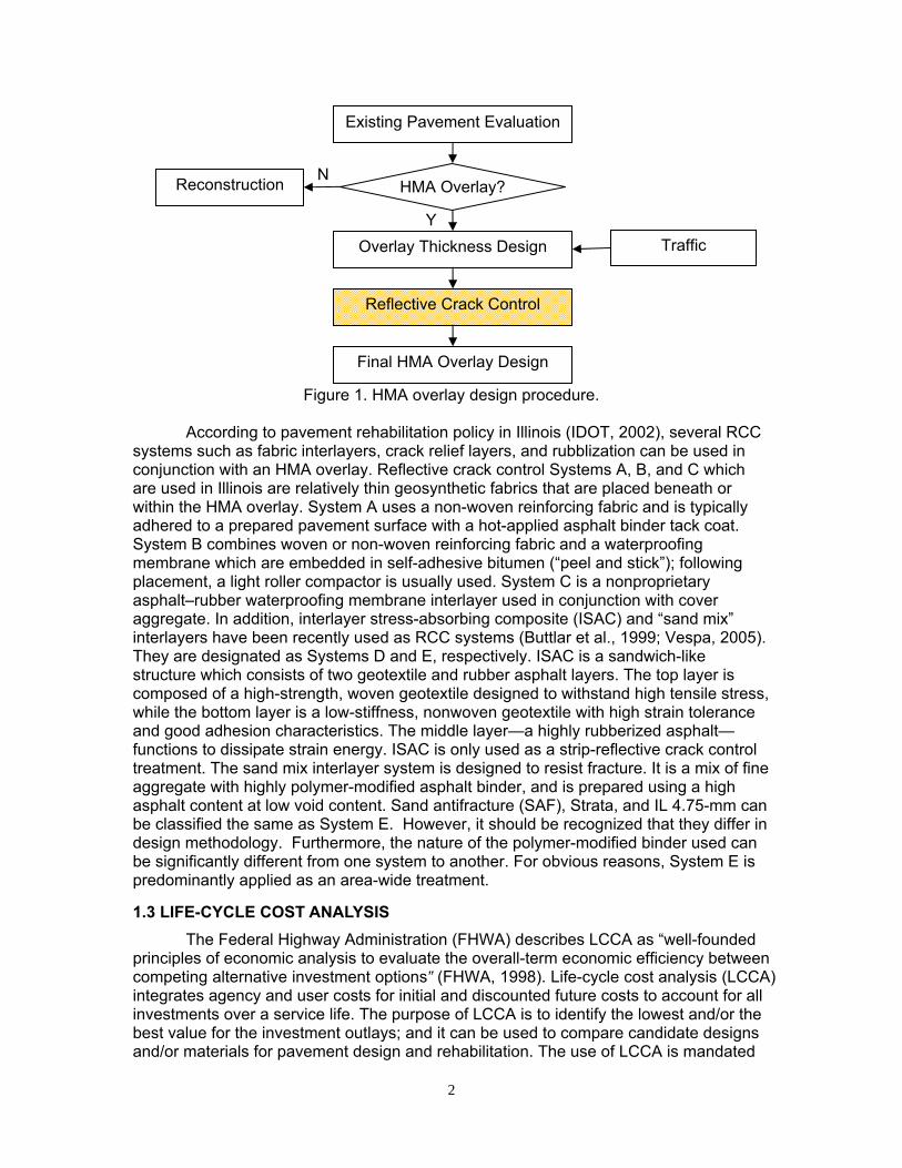
conditions (see Figure 1). After deciding overlay thickness, a suitable reflective crack control (RCC) system can be selected. The RCC system, however, does not affect the HMA overlay thickness, since it has no structural function. The RCC system is selected on the basis of how effectively it can reduce the occurrence of reflective cracking. The effectiveness of the RCC system depends not only on its performance, but also its cost efficiency. For example, if the cost of controlling reflective cracking and increasing the HMA overlay service life is relatively high compared to the cost of untreated overlay when considering the life-cycle cost analysis, then the approach is inefficient and the cost benefit could be high.

2

Figure 1. HMA overlay design procedure.

According to pavement rehabilitation policy in Illinois (IDOT, 2002), several RCC

systems such as fabric interlayers, crack relief layers, and rubblization can be used in conjunction with an HMA overlay. Reflective crack control Systems A, B, and C which are used in Illinois are relatively thin geosynthetic fabrics that are placed beneath or within the HMA overlay. System A uses a non-woven reinforcing fabric and is typically adhered to a prepared pavement surface with a hot-applied asphalt binder tack coat. System B combines woven or non-woven reinforcing fabric and a waterproofing membrane which are embedded in self-adhesive bitumen (“peel and stick”); following placement, a light roller compactor is usually used. System C is a nonproprietary asphalt–rubber waterproofing membrane interlayer used in conjunction with cover aggregate. In addition, interlayer stress-absorbing composite (ISAC) and “sand mix” interlayers have been recently used as RCC systems (Buttlar et al., 1999; Vespa, 2005). They are designated as Systems D and E, respectively. ISAC is a sandwich-like structure which consists of two geotextile and rubber asphalt layers. The top layer is composed of a high-strength, woven geotextile designed to withstand high tensile stress, while the bottom layer is a low-stiffness, nonwoven geotextile with high strain tolerance and good adhesion characteristics. The middle layer—a highly rubberized asphalt— functions to dissipate strain energy. ISAC is only used as a strip-reflective crack control treatment. The sand mix interlayer system is designed to resist fracture. It is a mix of fine aggregate with highly polymer-modified asphalt binder, and is prepared using a high asphalt content at low void content. Sand antifracture (SAF), Strata, and IL 4.75-mm can be classified the same as System E. However, it should be recognized that they differ in design methodology. Furthermore, the nature of the polymer-modified binder used can be significantly different from one system to another. For obvious reasons, System E is predominantly applied as an area-wide treatment.

1.3 LIFE-CYCLE COST ANALYSIS The Federal Highway Administration (FHWA) describes LCCA as “well-founded

principles of economic analysis to evaluate the overall-term economic efficiency between competing alternative investment options” (FHWA, 1998). Life-cycle cost analysis (LCCA) integrates agency and user costs for initial and discounted future costs to account for all investments over a service life. The purpose of LCCA is to identify the lowest and/or the best value for the investment outlays; and it can be used to compare candidate designs and/or materials for pavement design and rehabilitation. The use of LCCA is mandated

Existing Pavement Evaluation

Overlay Thickness Design

HMA Overlay?

Reflective Crack Control

Final HMA Overlay Design

Reconstruction

Traffic Y

N

3

by federal legislation such as the Intermodal Surface Transportation Efficiency Act (ISTEA) of 1991 and the National Highway System (NHS) Designation Act of 1995.

Three approaches have been used to evaluate cost effectiveness: maximum benefit, least cost, and a combination of the two (Lamptey et al., 2005). The maximum benefit approach is applicable for some activities such as capital investment for which the exact benefit is difficult to assess from alternatives due to uncertainty. In the least cost approach, when the same benefit can be achieved from each alternative, the least cost is regarded as the best. The third approach is the combination of benefit and cost analysis which was recommended by NCHRP Synthesis 223 (Geoffrey, 1996). This method is only applicable when both benefit and cost can be quantified in monetary terms.

In this study, the performance and cost benefit combination approach is used to evaluate the effectiveness of interlayer systems. The benefit of an interlayer system that results from the extension of service life of an HMA overlay can be assessed using field crack survey data. Cost benefit can then be quantified using LCCA, considering material costs, user delay costs, and overlay life (time to next rehabilitation). Subcategorization can also be considered, so that factors such as traffic level, climate, and PCC joint spacing on subsequent overlay deterioration rate can be considered in the LCCA.

1.4 DECISION-MAKING PROCEDURE IN PAVEMENT DESIGN To determine the optimal design from alternatives under consideration, a

decision-making procedure was required. Pavement evaluation considering performance and cost effectiveness is the most important step in this regard (Beg et al., 2000; Wei and Tighe, 2004; Lamptey et al., 2005). In Beg et al. (2000), three main components were used to evaluate pavement types: agency costs, user delay costs, and performance levels. In their study, the pavement performance levels were quantified from a pavement performance curve using a present serviceability index (PSI). Then, a cost-effectiveness index was developed using PSI, equivalent uniform annual cost (EUAC), performance period, and minimum tolerable PSI. In addition, other nonmonetary factors such as available materials and agency policy were included in the decision tree developed from their research. After combining the cost-effectiveness index and supplementary factors, the optimal pavement strategy could be selected.

For Wei and Tighe (2004), cost effectiveness (CE) was an essential parameter for selecting each treatment or strategy. The CE of each treatment was calculated based on performance effectiveness and corresponding life-cycle cost (LCC). Performance effectiveness was computed from the area under a performance curve for a treatment; LCC included agency and user costs for the treatment. Based on the CE analysis, the most cost-effective method was determined, and the best timing of the treatment was also decided. Finally, using the CE, strategy levels, and proper timing, a decision tree was developed to select the most appropriate treatment for a specific location and conditions.

In their study, Lamptey et al. (2005) developed a decision tree based on the cost effectiveness as well as the applicability of alternative designs. Figure 2 shows this decision tree for selecting an optimal pavement rehabilitation and maintenance (R&M) strategy simplified for Indiana pavement design procedures. In this procedure, the core part of the strategy is the LCCA evaluation of the R&M strategies.

4

Figure 2. Typical decision tree to select a pavement alternative (Lamptey et al., 2005).

2. INTERLAYER SYSTEM DECISION PROCEDURE

2.1 GENERAL PROCEDURE The procedure for selecting cost-effective interlayer systems consists of two main

parts: performance and cost-benefit analysis. Figure 3 shows an entire but simplified framework for decision making related to cost-effective interlayer systems. In the first step, the five types of interlayer systems previously mentioned are incorporated as HMA overlay alternatives. Then, the relative benefits of the alternatives are obtained and compared with an untreated HMA overlay. In the performance-benefit analysis, the performance-benefit ratio is obtained to represent the reflective cracking delay rate for each interlayer system, and consequently, how long the service life of the HMA overlay is extended. In the second step, LCCA is used to evaluate the cost effectiveness achieved by the interlayer system. Then, using a decision tree, an optimal interlayer can be selected for a given HMA overlay design based on the cost-benefit analysis, as well as compatibility with the HMA overlay design.

Pavement Definition

Pavement Design Alternatives Definition

R&M Strategies

LCCA Evaluation

Optimum R&D Strategy Decision

5

Figure 3. Framework for decision making for interlayer system evaluation to control

reflective cracking.

2.2 INTERLAYER SYSTEM PERFORMANCE EVALUATION In-situ effectiveness assessment of interlayer systems to control reflective

cracking was conducted as a basis of cost effectiveness evaluation (Al-Qadi et al., 2008). For the five types of interlayer systems used in Illinois, the extent and severity of reflective cracking was obtained from field data collected from a survey of 24 locations. Based on these data, the performance-benefit ratios (PBRs) were determined to quantify the relative benefit of these interlayer systems to an untreated HMA overlay. For System D, it was reported that the PBR decreases with the increase of annual equivalent single-axle loads (ESALs); statistically, the effect of ESALs on PBR was significant. In addition, lowest monthly average temperature, TL and joint spacing (JS) were important factors to the performance of System D. A regression model to predict the PBR of System D was developed (Table 1). However, for two area-type interlayer systems, System A and System E, in general, the PBR decreased insignificantly with the increase of ESALs. No obvious variables were found to affect the PBRs of area-type System A and System E. Thus, the average PBR can be used to represent the performance of these two interlayer systems despite having some variations: average PBR is 1.22 for area-type System A and 1.49 for System E. Table 1. Performance-Benefit Ratio Prediction Model for Interlayer System D (Al-Qadi et

al., 2008)

Interlayer system Performance-benefit ratio prediction model Eq.

System D (strip) PBR = 5.29 – 3.49 x 10-6 (ESALs) – 0.0854 (TL) – 0.0279 (JS) 1

Performance–Benefit Ratio

Field Crack Survey

Field Performance Data

Cost-Benefit Evaluation

Cost-Effectiveness Interlayer System Decision

LCCA

Decision Tree

Performance- benefit

analysis

Cost- benefit

analysis

6

2.3 LIFE-CYCLE COST ANALYSIS FOR HMA OVERLAYS In general, a standard LCCA procedure suggested by FHWA was used for this

project (FHWA, 1998). Two modules were added, specifically to consider interlayer systems used in HMA overlays. First, the service life of the HMA overlay with an interlayer system was estimated using the PBR of the interlayer system. Second, additional costs for installing the interlayer system were calculated based on unit price and quantity of the interlayer system. To compute life-cycle cost (LCC) of the HMA overlays with interlayer systems, monetary items such as agency cost, user cost, expenditure diagram, and net present value need to be clarified. Note in the description below that maintenance costs were not considered in this LCCA because they are not a large portion of the total cost, and it was assumed that the same types of routine maintenance, such as crack sealing, are usually scheduled for both control and treated sections. This assumption may decrease the cost effectiveness of interlayer systems when they demonstrate a positive performance benefit. Consequently, it may underestimate the cost effectiveness of the interlayer systems. This conservative approach, however, compensates for the uncertainty of the interlayer system performance based on field survey data from a small number of locations.

2.3.1 Agency Cost

Agency cost comprises all costs of HMA overlay and interlayer systems, including materials and construction. For the HMA, it covers initial and successive HMA overlays needed for the pavement analysis period. Corresponding to HMA overlay design, a quantity of the HMA overlay per lane-mile is computed for the thickness of wearing surface and leveling binder. The unit price of the HMA overlay is expressed as $/ton, and it is converted into $/ft2/in using a constant density of 150 lb/ft3. This analysis does not take into account any milling, patching, crack sealing, and other rehabilitation activities prior to the overlay. Nonetheless, existing pavements should be carefully treated to ensure the performance of the overlay and interlayer systems.

When an interlayer system is used in the HMA overlay, a supplemental cost for the interlayer system is calculated per lane-mile based on the number of strips for strip-type interlayer systems or applied area for area-wide interlayer systems. For strip-type interlayer systems, when the number of strips is the same as the number of joints—that is, the strips are installed only on joints— the number of strips is indirectly determined from joint spacing of an existing jointed concrete pavement (JCP). Otherwise, the number of strips can be directly determined. Thus, unit price is $/strip. For area-wide interlayer systems, two approaches are used. Unit price and installation cost of System A are $/ln.ft and $/100 ft, respectively; while System E has the same units as HMA overlay, since it is a mixture-type interlayer system.

2.3.2 User Cost

In general, the components of user cost are user delay cost, vehicle operating cost (VOC), and crash cost (FHWA, 1998). The analysis of this research basically followed the one used in RealCost 2.2 to compute user cost. Input items to compute user cost are traffic characteristics, work zone characteristics, and value of travel time. The traffic characteristics are specified by annual average daily traffic (AADT); percentage of passenger cars, single-unit, and combination trucks; and hourly distributions in urban or rural areas, or both. In these calculations, AADT distribution is determined only for principal arterial roads; neither interstates nor minor arterials are considered. The work zone is characterized using work zone length and time, speed

7

change, stopping, and queue idling delay, and VOC. Truck equivalent factors are determined to calculate road capacity assuming that the grade of the road is less than 2%. Regarding the value of travel time, base case values provided in 1996 dollars in the FHWA bulletin (FHWA 1998) are converted into values corresponding to a specific year using an escalation factor. Using a consumer price index (CPI) (U.S. Department of Labor 2008), the escalation factor is computed as a CPI ratio of 1996 to a certain year, as shown in Figure 4.

Figure 4. Escalation value variation with base year 1996.

2.3.3 Expenditure Diagram

For two overlay strategies of control and treated sections, pavement condition variations and expenditure diagrams are depicted in Figure 5. For the untreated overlay, the pavement condition drops relatively faster than for a treated section and reaches a trigger value at TA. On the other hand, the treated section has a longer service life (TB – T0 ) than that of the untreated section (TA – T0). When the shorter service life of TA – T0 is used as an analysis period in LCCA, the treated overlay is still in a good condition at the end of the analysis period and has a remaining service life of (TB – TA). The expenditure diagrams of the overlays are constructed for the one cycle of untreated overlay service life. Since no maintenance is considered, only initial overlay construction and user cost are included in the expenditure diagram. However, to compensate for the remaining service life of the treated overlay, a salvage value is considered as a negative cost. The salvage value is a portion of the initial cost of the treated overlay; and is proportional to the ratio of the remaining service life (TB – TA) to the original service life span (TB – T0), as shown in Figure 5(b). The longer the service life of the treated section is, the larger the salvage value becomes. When multiple overlays are constructed, a salvage value is computed based on the last overlay span.

0.00

0.25

0.50

0.75

1.00

1.25

1.50

1984 1988 1992 1996 2000 2004 2008

Year

Elev

atio

n

8

Figure 5. (a) Pavement condition variation over pavement age and (b) expenditure

diagram corresponding to one cycle.

2.3.4 Net Present Value and Equivalent Uniform Annual Cost

When initial and future costs are summed in LCCA, the future cost should be discounted to the base year by means of a discount rate. The discount rate incorporates interest rate and inflation rate. Generally, the discount rate used in pavement analysis ranges from 3.0% to 5.0%. IDOT adopted the discount rate of 3.0% as a default value in LCCA. A net present value (NPV) is the sum of the initial value and the discounted values as follows:

∑ ⎟⎠⎞

⎜⎝⎛

++=

n

i11tscoFuturetscoInitialNPV (2)

where,

NPV is net present value; and n is an expenditure year.

In this equation, no discount rate is applied to the initial cost, and a constant discount rate is applied to additional multiple overlays, as well as the salvage value. For each overlay, NPV can be broken down into agency and user costs, as well as salvage value, as follows:

A

B

Time

Pavement Condition

Trigger

Agency cost A

User cost A

Cost

Pavement age

TB

Overlay

Agency cost B

User cost B

TA

Analysis period

Analysis period

A: Untreated section B: Treated section with an interlayer system

Multiple overlays

Salvage value B = Initial agency cost B TB - TA

TB - T 0

T0

Salvage value B

(a)

(b)

9

AAAA tscoUsertscoAgencytscoInitialNPV +== (3)

( )0A TT

BBB 03.011valueSalvagetscoInitialNPV

-

⎟⎠⎞

⎜⎝⎛

++=

(4)

Finally, equivalent uniform annual cost (EUAC) is determined based on NPV, the discount rate, and the number of years into future (n) as follows:

( )

( ) ⎥⎥⎦

⎤

⎢⎢⎣

⎡

−+

+=

1i1i1iNPVEUAC n

n

(5)

2.4 COST-EFFECTIVE INTERLAYER SYSTEM DECISION PROGRAM (CIND) A special-purpose LCCA was developed to determine the cost effectiveness of

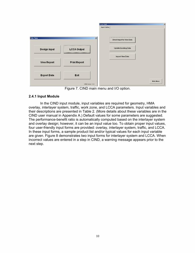
interlayer systems in HMA overlays: the cost-effective interlayer system decision program (CIND). The LCCA procedure employed in CIND to compute LCC is similar to the approach in RealCost Version 2.2 developed by FHWA (FHWA, 1998). CIND is composed of three modules, shown in Figure 6: input, analysis, and output. In addition, a file input/out (I/O) menu is also provided to import an existing data file or to save current data. Figure 7 shows a main menu of CIND and an I/O option in the design input module. Details of the CIND operation are described in Appendix A (User Manual for CIND Version 1.0).

Figure 6. Framework for the Cost-effective INterlayer selection Decision program

(CIND).

Input

HMA Overlay

Interlayer

Traffic

Analysis

Agency Cost

User Delay Cost

Output

Grand Total Cost

Cost-Effective Interlayer System

Evaluation

Material price Construction period Lane configuration

Material cost Construction period

Service life

AADT

Overlay cost Interlayer cost Salvage value

Free flow cost Forced cost

Salvage value Default values

Agency cost User delay cost

Net present value Expenditure diagram

LCCA Parameters

Performance- benefit ratio

10

Figure 7. CIND main menu and I/O option.

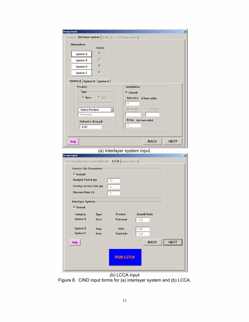
2.4.1 Input Module

In the CIND input module, input variables are required for geometry, HMA overlay, interlayer system, traffic, work zone, and LCCA parameters. Input variables and their descriptions are presented in Table 2. (More details about these variables are in the CIND user manual in Appendix A.) Default values for some parameters are suggested. The performance-benefit ratio is automatically computed based on the interlayer system and overlay design; however, it can be an input value too. To obtain proper input values, four user-friendly input forms are provided: overlay, interlayer system, traffic, and LCCA. In these input forms, a sample product list and/or typical values for each input variable are given. Figure 8 demonstrates two input forms for interlayer system and LCCA. When incorrect values are entered in a step in CIND, a warning message appears prior to the next step.

11

(a) Interlayer system input.

(b) LCCA input

Figure 8. CIND input forms for (a) interlayer system and (b) LCCA.

12

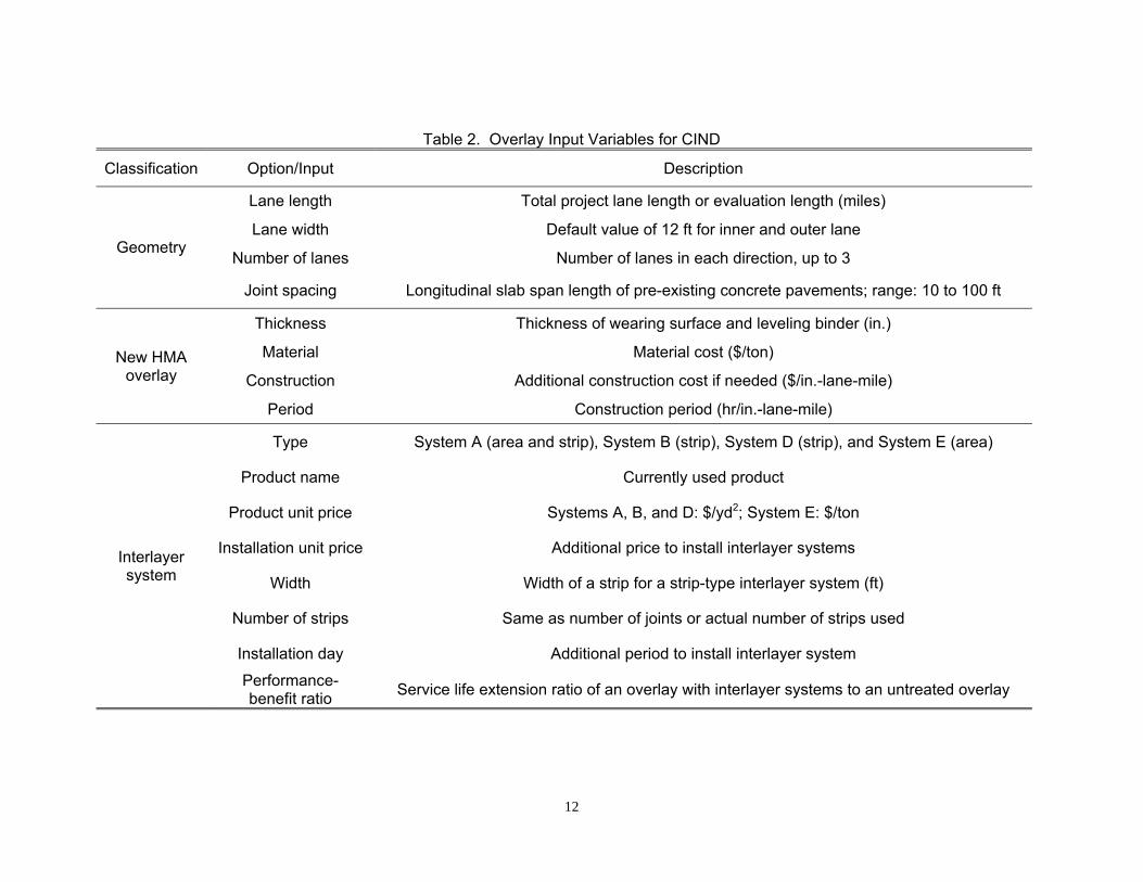
Table 2. Overlay Input Variables for CIND

Classification Option/Input Description

Geometry

Lane length Total project lane length or evaluation length (miles)

Lane width Default value of 12 ft for inner and outer lane

Number of lanes Number of lanes in each direction, up to 3

Joint spacing Longitudinal slab span length of pre-existing concrete pavements; range: 10 to 100 ft

New HMA overlay

Thickness Thickness of wearing surface and leveling binder (in.)

Material Material cost ($/ton)

Construction Additional construction cost if needed ($/in.-lane-mile)

Period Construction period (hr/in.-lane-mile)

Interlayer system

Type System A (area and strip), System B (strip), System D (strip), and System E (area)

Product name Currently used product

Product unit price Systems A, B, and D: $/yd2; System E: $/ton

Installation unit price Additional price to install interlayer systems

Width Width of a strip for a strip-type interlayer system (ft)

Number of strips Same as number of joints or actual number of strips used

Installation day Additional period to install interlayer system

Performance- benefit ratio Service life extension ratio of an overlay with interlayer systems to an untreated overlay

13

Table 2 (continued). Overlay Input Variables for CIND

Category Option/Input Description

Traffic

Category Urban or rural

Priority Principal arterial or minor arterial (no interstate)

Current year First year of the analysis period

AADT Annual average daily traffic (AADT) in both directions in current year

Road class Illinois road classifications regarding traffic volume and number of lanes

Growth rate Annual traffic growth rate of AADT (same rate for all vehicles)

Passenger cars % of passenger cars in the AADT

Single-unit trucks % of single-unit trucks in the AADT

All other trucks % of combination trucks in the AADT

Work zone

Lane opening in work zone Number of lanes open in work zone area in each direction, up to two lanes

Upstream speed Speed limit in normal operation (mph)

Work zone speed Speed limit in work zone area (mph)

Work zone Length Maximum length of work zone area when vehicle speed is reduced (miles)

Work zone duration Duration for work zone (”all day” option is used as default).

Life-cycle cost

analysis parameters

Analysis period Total design year to be analyzed (year), up to 50 years

Overlay service life Overlay service life span with no interlayer system (year)

Discount rate Rate for discounting future costs to present value (3% to 5%)

14

2.4.2 Output Module

Using the input variables in the previous section, LCCA is performed to compute agency and user costs for one cycle of the untreated HMA overlay service life, as well as for a total design analysis period. For the one-cycle period, agency cost, user cost, and salvage value are compared for each HMA overlay design to easily obtain the cost reduction when interlayer systems are used. The relative cost benefit of interlayer systems is computed for the total design analysis period based on a ratio of total cost of the treated overlay to that of the untreated HMA overlay. The LCCA results are presented in the output module as a summary report and five charts for the LCC components.

The cost benefit of an interlayer system is defined as a ratio of EUAC saved through the use of the interlayer system to EUAC of an HMA overlay without interlayer systems (see Equation 10); so-called a benefit-cost ratio (B/C). From LCCA, the EUAC of each HMA overlay is obtained based on the PBR of interlayer systems used in the HMA overlays and the material costs of the HMA overlays and the interlayer systems. Figure 9 presents a typical B/C output for four interlayer systems.

100C

CC(%)C/B

U

TU ×−

= (6)

where,

B/C is a benefit-cost ratio as a percentage; and CU and CT are EUAC of an untreated and treated overlay for a design life span.

Figure 9. CIND output form demonstrating a benefit-cost ratio.

15

3. EVALUATION OF COST EFFECTIVENESS OF INTERLAYER SYSTEMS

3.1 COST BENEFIT For 25 interlayer systems, cost effectiveness was evaluated using a benefit-cost

ratio (B/C). The material costs of the interlayer systems and HMA overlays are listed in Table 3. Since material prices vary locally depending on the quantity of materials, manufacturers, and other factors, the average values obtained from available sources were used for this evaluation. According to Buttlar et al. (2000), fabric cost was categorized in terms of quantity. For low, medium, and high quantity, the fabric cost was $1.23, $0.84, and $0.65/yd2 for area-type System A and $0.51, $0.30, and $0.23/ln.ft for strip-type System A. According to one manufacturer, System B was $0.89/ft2 and System D (ISAC) was $2.39/ft2. For mixture costs, IDOT provided numbers for four projects constructed in 2003: IL 130 Philo, IL 17 Aledo, IL 117 Benson, and IL 76 Belvidere. For the four projects, the average cost was $49.30/ton for IL 4.75-mm mix, $38.60/ton for IL 9.5-mm mix, and $38.20/ton for surface mix. The reference year, in terms of when those interlayer systems’ costs were surveyed, does not coincide with the evaluation year for each project. Therefore, these reference year costs were converted to correspond with each evaluation year using the escalation factors shown in Appendix B. There are some limitations, however, in using these sources to represent real and current market prices of materials. For this reason, the effect of material prices on benefit -cost are analyzed later to validate the benefit-cost analysis and to reflect the variability of the material prices.

16

Table 3. Material Prices for Evaluated Interlayer Systems

Material Unit price Unit Reference

year

HMA Overlay

Wearing surface Mix “D” 38.2 $/ton 2003

Leveling binder IL9.5 38.6 $/ton

Interlayer System

System A Area

<20,000 1.23 $/yd2

2000 20,000- 70,000 0.84 $/yd2

>70,000 0.65 $/yd2

System A Strip

<18,000 0.51 $/ln.ft

2000 18,000-100,000 0.30 $/ln.ft

>100,000 0.23 $/ln.ft

System B Strip PavePrepSA Roadtac 8.01 $/yd2 2008

System D Strip ISAC 21.5 $/yd2 2008

System E Area

IL130 61.0 $/ton

2003

IL17 51.8 $/ton

IL117 44.1 $/ton

IL76 40.3 $/ton

Average 49.3 $/ton

3.1.1 System A (Area)

Figure 10 shows B/C at various PBR values and three cost levels for the area-type System A. B/C variation is in the range of ±20% at each cost level due to various PBR values of the interlayer systems. In addition, the B/C decreases with the increase of the cost level. To achieve positive cost effectiveness, then, an area-type System A should have a marginal level of performance, as well as lower cost. When the System A has a medium level cost of $0.84/yd2, for example, a minimum PBR of 1.3 is required for the system to be cost effective (Figure 11). Thus, despite a positive PBR value, cost effectiveness of the system cannot be achieved unless material cost becomes cheaper than a truncate value. For a given set of traffic and environmental conditions at a location, the performance of the interlayer system can be estimated and consequently, the truncate material cost can be determined. If an area-type System A interlayer that is cheaper than truncate cost is available locally, the System A can be cost effective. (Detailed LCCA results are shown in Appendix B.)

17

Figure 10. B/C of area-type System A with respect to PBR and cost level.

Figure 11. Minimum PBR at three material cost levels for area-type System A.

3.1.2 System A (Strip) and System B

According to field evaluations, the PBRs of strip-type System A and System B (Al-Qadi et al., 2008) are always equal to or less than 1.0 at five surveyed locations: 0.65, 0.35, and 0.80 for the System A; and 1.0 and 0.93 for the System B. Regardless of the systems’ material costs, they cannot be considered cost effective because the PBR values are negative or, at most, equal to one.

-40

-30

-20

-10

0

10

20

30

0.0 0.5 1.0 1.5 2.0

B/C

(%)

PBR

System A (area)

1.24 1.301.40

0.0

0.5

1.0

1.5

2.0

Low Medium High

PBR

Material cost level

System A (area)

Low cost

Medium

High

18

3.1.3 System D

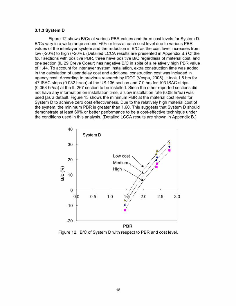
Figure 12 shows B/Cs at various PBR values and three cost levels for System D. B/Cs vary in a wide range around ±5% or less at each cost level due to various PBR values of the interlayer system and the reduction in B/C as the cost level increases from low (-20%) to high (+20%). (Detailed LCCA results are presented in Appendix B.) Of the four sections with positive PBR, three have positive B/C regardless of material cost, and one section (IL 29 Creve Coeur) has negative B/C in spite of a relatively high PBR value of 1.44. To account for interlayer system installation, extra construction time was added in the calculation of user delay cost and additional construction cost was included in agency cost. According to previous research by IDOT (Vespa, 2005), it took 1.5 hrs for 47 ISAC strips (0.032 hr/ea) at the US 136 section and 7.0 hrs for 103 ISAC strips (0.068 hr/ea) at the IL 267 section to be installed. Since the other reported sections did not have any information on installation time, a slow installation rate (0.08 hr/ea) was used [as a default. Figure 13 shows the minimum PBR at the material cost levels for System D to achieve zero cost effectiveness. Due to the relatively high material cost of the system, the minimum PBR is greater than 1.60. This suggests that System D should demonstrate at least 60% or better performance to be a cost-effective technique under the conditions used in this analysis. (Detailed LCCA results are shown in Appendix B.)

Figure 12. B/C of System D with respect to PBR and cost level.

-20

-10

0

10

20

30

40

0.0 0.5 1.0 1.5 2.0 2.5 3.0

B/C

(%)

PBR

System D

Low cost Medium High

19

Figure 13. Minimum PBR at three material cost levels for System D.

3.1.4 System E

Based on material cost in four projects from 2003, the average unit price of IL 4.75-mm mixtures used as System E is $49.3/ton, ranging from $40.3 to $61.0/ton; that of IL 9.5-mm mixtures as a conventional leveling binder mixture is $38.6/ton, and that of wearing surface mixtures is $38.2/ton. In each project, the total cost ratio of the treated to untreated overlay is constant (around 1.09), though each material cost is different. In addition, no material cost information was available for two other sections for which different types of materials (sand anti-fracture, SAF) were used. The same average material cost for IL 4.75-mm mixtures was used for these two sections. Thus, B/C was investigated with respect to PBR at the three material cost levels: high (20% above the medium), medium, and low (20% below medium). Detailed LCCA results are presented in Appendix B.

1.601.69

1.80

0.0

0.5

1.0

1.5

2.0

Low Medium High

PB

R

Material cost level

System D

20

Figure 14Figure 14 shows the B/C variation for the three material cost levels with

respect to PBR of the six projects. The B/C decreases with the decrease of PBR, but it is greater than zero for all cases except one whose material cost is high and PBR is relatively low. The minimum PBR corresponding to zero B/C is presented for each material cost level in Figure 15. At the medium and high material cost levels, System E can be cost effective when it has a minimum performance benefit ratio of 1.08 and 1.21, respectively. The minimum PBR is less than 1.0 for the low material cost level in which System E is cheaper than the leveling binder, but it is not possible. The main reasons why System E is cost effective are that System E has higher PBR, lower material cost, and no installation cost.

-20

0

20

40

60

80

0.0 1.0 2.0 3.0 4.0

B/C

(%)

PBR

System E

21

Figure 14. B/C of System E with respect to PBR.

Figure 15. Minimum PBR at three material cost levels for System E.

3.2 COST-EFFECTIVENESS EVALUATION OF THE INTERLAYER SYSTEMS The cost effectiveness of interlayer systems was evaluated for the short- and

long-term periods. Crack survey and performance benefit analysis of the interlayer systems were conducted for their in-service life, mostly less than ten years. Since no multiple overlays were considered in developing the PBR, overlays added in the future were not included in this LCCA. Hence, LCC of the overlay was determined for a

-20

0

20

40

60

80

0.0 1.0 2.0 3.0 4.0

B/C

(%)

PBR

System E

System E

0.911.08

1.21

0.0

0.5

1.0

1.5

2.0

Low Medium HighMaterial cost level

PBR

Low cost Medium High

22

relatively short-term period. In addition, under the assumption that subsequent overlays can perform as well as previous ones, LCCA was conducted to evaluate the cost effectiveness for a period of 30 years. Such a long-term evaluation can be of use to standardize cost effectiveness with respect to overlay service life and analysis period, which is different for each project.

3.2.1 Short-Term Evaluation

Cost effectiveness of the interlayer systems was evaluated based on performance and cost benefit. As mentioned, no interlayer system could be systematically cost effective unless the PBR of the interlayer system is greater than 1.0. Cost effectiveness only for interlayer systems with positive PBR was examined by means of B/C obtained at the medium material cost level. The evaluation results are summarized in Table 4. Using B/C as well as PBR, cost effectiveness was grouped into three categories: “inefficient,” “insignificant,” and “efficient”. Within the inefficient group with negative B/C (designated “X” in Table 4), an interlayer system whose PBR is even less than1.0 is downgraded into a “too inefficient” level (designated “XX” in Table 4). The insignificant group (designated “Δ” in Table 4) has positive B/C, but the B/C is less than 10%, which cannot unconditionally guarantee the cost effectiveness of an interlayer system. When local material costs increase during a bidding process, the marginal cost benefit could be negative. In the IL148 Christopher section, for instance, B/C at the medium material cost level is positive (1.9%), but it becomes negative (-4.8%) at the high material cost level. Thus, interlayer systems in the insignificant group are only conditionally cost effective. The efficient group (designated “O” in Table 4) has 10% B/C or greater at the medium material cost level and B/C is unconditionally positive regardless of material cost variation. For example, the IL40 Deer Grove section demonstrates B/C of 10.4%, 16.0%, and 18.7% at high, medium, and low material cost levels, respectively. In cases in which B/C is over 20%, an interlayer system is absolutely regarded as a very cost-effective alternative system (designated “OO” in Table 4).

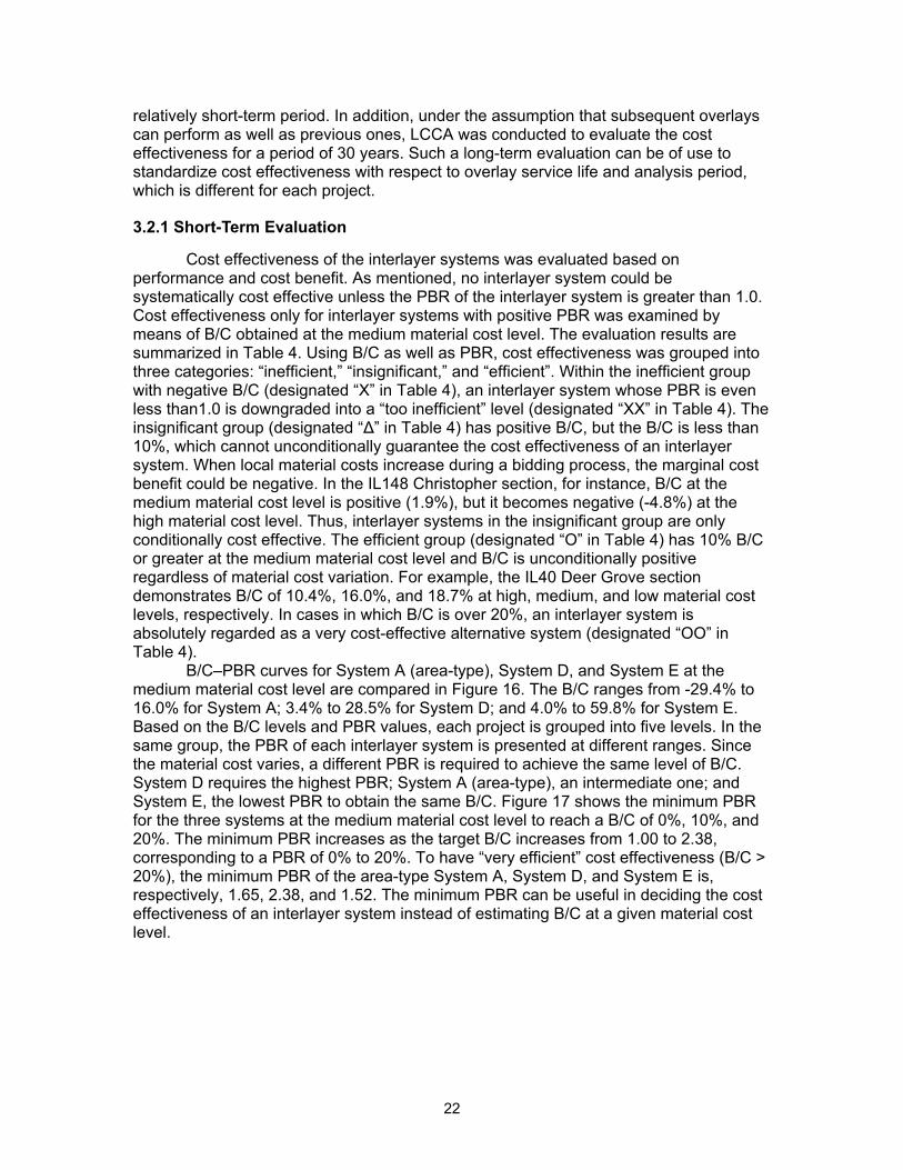
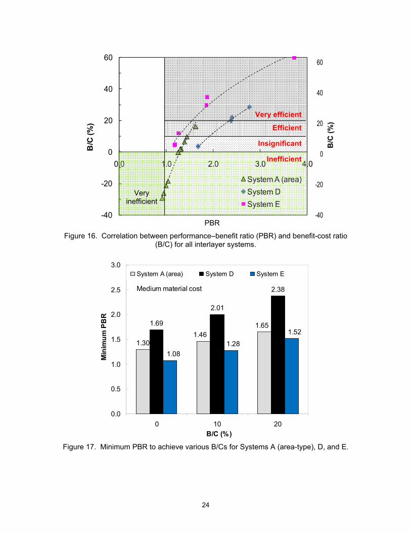
B/C–PBR curves for System A (area-type), System D, and System E at the medium material cost level are compared in Figure 16. The B/C ranges from -29.4% to 16.0% for System A; 3.4% to 28.5% for System D; and 4.0% to 59.8% for System E. Based on the B/C levels and PBR values, each project is grouped into five levels. In the same group, the PBR of each interlayer system is presented at different ranges. Since the material cost varies, a different PBR is required to achieve the same level of B/C. System D requires the highest PBR; System A (area-type), an intermediate one; and System E, the lowest PBR to obtain the same B/C. Figure 17 shows the minimum PBR for the three systems at the medium material cost level to reach a B/C of 0%, 10%, and 20%. The minimum PBR increases as the target B/C increases from 1.00 to 2.38, corresponding to a PBR of 0% to 20%. To have “very efficient” cost effectiveness (B/C > 20%), the minimum PBR of the area-type System A, System D, and System E is, respectively, 1.65, 2.38, and 1.52. The minimum PBR can be useful in deciding the cost effectiveness of an interlayer system instead of estimating B/C at a given material cost level.

23

Table 4. Summary of Cost-Effectiveness Evaluation of the Interlayer Systems Interlayer system Location PBR B/C (%) Cost

Effectiveness* High Medium Low

System A (area)

IL 148 Christopher 1.32 -4.8 1.9 5.2 Δ

IL 251 N. of US30 1.44 4.5 9.6 12.1 Δ

IL 29 Chillicothe 0.95 -34.2 -26.3 -22.4 XX

IL 9 E. of IL41 1.04 -28.1 -18.5 -14.0 X

IL 29 Mossville 0.92 -37.5 -29.4 -25.4 XX

IL 40 Deer Grove 1.63 10.4 16.0 18.7 O

US 34 Mendota 1.26 -7.0 -0.3 3.0 X

US 136 E. San Jose 1.39 -0.3 6.4 9.6 Δ

IL 111 Pontoon Beach 1.00 -29.1 -21.6 -17.9 X

System A (strip)

IL 130 Villa Grove 0.80 - - - XX

IL 178 Oglesby 0.65 - - - XX

US 34 Kirkwood 0.35 - - - XX

Mattis Ave. 0.98 - - - XX

System B IL 29 Creve Coeur 1.02 - - - X

Mattis Ave. 0.93 - - - XX

System D

IL 29 Creve Coeur 1.44 -13.3 -9.77 -6.52 X

Mattis Ave. 2.77 26.3 28.5 30.7 OO

US136 E. San Jose 2.40 17.5 21.6 25.8 OO

IL 267 Greenfield 2.38 15.4 19.7 24.0 O

System E

IL 76 Belvidere 1.17 -3.0 4.0 11.1 Δ

IL 17 Aledo 3.73 6.1 59.8 63.0 OO

IL 117 Benson 1.88 29.6 34.6 39.6 OO

IL 130 Philo 1.27 5.4 11.9 22.1 O

US 136 E. San Jose 1.85 24.6 29.4 35.2 OO

US 136 W. San Jose 1.28 1.7 8.7 15.7 Δ

* XX: too inefficient (PBR < 1.0), X: inefficient (B/C ≤ 0%), Δ: insignificant (0% < B/C ≤ 10%), O: efficient (10% < B/C ≤ 20%), and OO: very efficient (B/C > 20%)

24

Figure 16. Correlation between performance–benefit ratio (PBR) and benefit-cost ratio

(B/C) for all interlayer systems.

Figure 17. Minimum PBR to achieve various B/Cs for Systems A (area-type), D, and E.

-40

-20

0

20

40

60

0.0 1.0 2.0 3.0 4.0

B/C

(%)

BRP

System A (area)System DSystem E

-40

-20

0

20

40

60

Medium material cost

1.30

1.69

2.01

2.38

1.461.65

1.081.28

1.52

0.0

0.5

1.0

1.5

2.0

2.5

3.0

0 10 20B/C (%)

Min

imum

PB

R

System A (area) System D System E

Very efficient

Efficient

Insignificant

Inefficient

Very inefficient

B/C

(%)

PBR

25

3.2.2 Long-Term Evaluation

The cost effectiveness of interlayer systems was investigated for a long-term period of 30 years. A control HMA overlay is assumed to have a service life of 10 years, so a total of three untreated consecutive overlays was considered for this purpose. A treated HMA overlay with an interlayer system has a longer service life proportional to its performance-benefit ratio. If the PBR is high enough, the treated overlay can be cost effective due to a smaller number of overlay constructions, as well its salvage value at the end of the analysis period. On the other hand, in the short-term cost-effectiveness evaluation, all cost benefit results from the salvage value, which could account for the relative extension of the overlay service life. Thus, in the long-term evaluation, except for the overlay service life and analysis period, the other variables were the same as for the short-term cost-effectiveness evaluation at the medium material cost level.

Table 5 lists the results of the short-term and long-term cost-effectiveness evaluation for 19 projects. Long-term B/Cs are greater than short-term B/Cs in 11 projects and are smaller than the short-term B/Cs in the other eight projects. Nonetheless, the same cost-effectiveness evaluation level could be achieved in 16 out of 19 projects: Only three projects, highlighted in boldface in the table, have different CE evaluation. System A at IL 251 section is at the “insignificant” level (9.6% of B/C) in the short-term cost effectiveness evaluation; while it is classified at the “effective” level (15.4% of B/C) in the long-term cost-effectiveness evaluation. Similarly, System D at IL 267 section is at the “effective” level in the short-term cost-effectiveness evaluation; but it is upgraded to the “very effective” level in the long-term cost-effectiveness evaluation. However, these level upgrades are not critical, as their B/Cs of 9.6% and 19.7% in the short-term evaluation are very close to the trigger values of 10% and 20%, respectively. Thus, the salvage value used in the short-term evaluation can be considered to accurately reflect the cost benefit of interlayer systems in the long-term evaluation. In spite of there being a few differences, the outcomes of the short-term and long-term evaluations both are acceptable enough to use for the cost-effectiveness evaluation of interlayer systems.

26

Table 5. Summary of Cost-Effectiveness Evaluation of the Interlayer Systems

Interlayer system Location PBR

Short-term (in-service)

Long-term (30yr)

B/C (%) CE B/C (%) CE

System A (area)

IL 148 Christopher 1.32 1.9 Δ 3.1 Δ

IL 251 N. of US30 1.44 9.6* Δ 15.4 O

IL 29 Chillicothe 0.95 -26.3 XX -33.8 XX

IL 9 E. of IL41 1.04 -18.5 X -17.4 X

IL 29 Mossville 0.92 -29.4 XX -35.2 XX

IL 40 Deer Grove 1.63 16.0 O 19.8 O

US 34 Mendota 1.26 -0.3 X -0.3 X

US 136 E. San Jose 1.39 6.4 Δ 9.4 Δ

IL 111 Pontoon Beach 1.00 -21.6 X -22.4 X

System D

IL 29 Creve Coeur 1.44 -9.77 X -4.7 X

Mattis Ave. 2.77 28.5 OO 35.3 OO

US 136 E. San Jose 2.40 21.6 OO 27.1 OO

IL 267 Greenfield 2.38 19.7 O 27.3 OO

System E

IL 76 Belvidere 1.17 4.0 Δ 2.6 Δ

IL 17 Aledo 3.73 59.8 OO 56.7 OO

IL 117 Benson 1.88 34.6 OO 33.3 OO

IL 130 Philo 1.27 11.9 O 10.5 O

US 136 E. San Jose 1.85 29.4 OO 31.7 OO

US 136 W. San Jose 1.28 8.7 Δ 11.7 O * Note that the long- and short-term evaluations yield different cost effectiveness.

27

4. DEVELOPMENT OF A B/C PREDICTION MODEL

4.1 B/C VARIABLES Numerous variables influence the B/C of interlayer systems. These variables can

be categorized into two groups, interlayer system variables and LCCA variables. Figure 18 illustrates the two groups of variables considered in the B/C prediction model. The interlayer system variables describe the features of each interlayer system and overlay in terms of performance-benefit ratio (PBR), material cost ratio (MCR), and construction time ratio (CTR). As mentioned, PBR represents the performance of interlayer systems in extending the service life of the treated overlay. PBR is determined using ESALs, TL, and JS. MCR and CTR are used to specify the relative material cost and construction time of the treated overlay. MCR is calculated using interlayer system and overlay unit price (C), overlay thickness (H), and joint spacing (JS) for System D only. CTR is a function of construction time (T) and two geometric variables, H and JS. A discount rate is used to calculate future agency and user costs. In addition, work zone characteristics and other cost- and traffic-related parameters can be classified into the LCCA variables.

A representative HMA overlay pavement commonly used in Illinois was used to develop a B/C prediction model. Among various overlay designs surveyed in this project, the majority of overlays consisted of a 1.5-in.-thick wearing surface and a 0.75-in.-thick leveling binder, which was placed over a composite pavement with 30-ft joint spacing (Figure 19). System A (area-type) and System E were placed under the leveling binder and System E was substituted for the leveling binder. The PBR of the interlayer system was calculated using the PBR prediction models for System A (area-type), System D, and System E, respectively. To cover the field performance evaluation of each interlayer system, the B/C prediction model was developed for a wide range of PBRs, from 0.9 to 3.0.

28

Figure 18. Main variables of a B/C prediction model.

Figure 19. Representative HMA overlay and interlayer systems.

4.1.1 Material Cost Ratio

In LCCA, the major agency cost is the material cost needed over the analysis period. The total cost of a new HMA overlay per mile-lane is simply computed by multiplying layer thickness and the unit price of the overlay for a mile-lane. When an

1.5 in. wearing surface

0.75 in. leveling binder

System A (area)

0.75 in. leveling binder

System D

System E

1.5 in. wearing surface

1.5 in. wearing surface

Interlayer system variables

Cost Effectiveness (B/C)

Performance-Benefit Ratio (PBR)

Material Cost Ratio (MCR)

Traffic (ESALs) Temperature (TL)

Material Cost: Wearing surface (CWS) Leveling binder (CLB)

Interlayer system (CIN) Geometry:

Thickness (HWS, HLB) Joint spacing (JS)

Traffic volume (AADT) Discount rate = 3%

Design analysis period = 30 years Work zone (vehicle speed, WZ length)

Road category (rural/urban, primary arterial)

Construction Time Ratio (CTR)

Construction Time: Wearing surface (TWS) Leveling binder (TLB)

Interlayer (TIS) Geometry:

Thickness (HWS, HLB) Joint spacing (JS)

LCCA variables

29

interlayer system is incorporated, the interlayer systems’ cost is added accordingly. While area-type System A is placed over the whole area under HMA overlay, System D strips are applied only over discontinuities of existing pavements, as shown in Figure 19. Hence, the quantity of strip-type interlayer systems depends on the number of discontinuities and strip width. Since the width of System D is generally 3 ft and the strips are usually installed on joints, the quantity of the strips can be determined by means of joint spacing (JS). For System E, the system replaces the leveling binder.

Material cost ratio (MCR) is defined as a ratio of unit material cost for a one-lane, 1.0-mile-long (5280 ft), (12 ft-wide-) HMA overlay, which includes an interlayer system, to that for an overlay without an interlayer system. For each interlayer system, MCR is calculated as follows: For the area-type System A,

( )( )

LBLBWSWS

INAALBLBWSWS

LBLBWSWS

INAALBLBWSWSAA

HCHCCHCHC

HCHCCHCHC

MCR

×+×+×+×

=

)3/5280×4(××+×)9/5280×4(×+)3/5280×4(××+×

=

(7)

For the System D,

( ) ( ) ( ) ( )( ) ( )

( )LBLBWSWS

INAALBLBWSWS

LBLBWSWS

INDLBLBWSWSD

HCHCJSCHCHC

xHCHCJSCxHCHC

MCR

×+×/3×+×+×

=

3/52804××+×/5280×4×+3/52804××+×

=(8)

For the System E,

LBLBWSWS

LBINEWSWSE HCHC

HCHCMCR

×+××+×

= (9)

where,

MCRAA, MCRD, and MCRE are material cost ratio for System A (area), System D, and System E, respectively; CWS and CLB are unit price of wearing surface and leveling binder whose unit price is converted from $/ton into $/yd2-in by multiplying 0.05625 (= ton/yd2-in. = [1ton/2000lbs] x [150lbs/ft3] x [9ft2/yd2] x [1ft/12in.]); CINAA, CIND, and CINE are unit price of interlayer systems in $/yd2, $/yd2, and $/yd2-in. for the Systems A, D, and E, respectively; HWS and HLB are thickness of wearing surface and leveling binder in inch; and JS is joint spacing in ft.

According to the material costs used in the field evaluation, MCRAA is 1.27, 1.18,

and 1.14 for high, medium, and low material cost levels, respectively, of area-type System A. This suggests, for example, that when medium material cost-level System A (area) is used, the material cost increases 18% compared to untreated overlay. For System D, MCRD is 1.39, 1.32, and 1.26 for the three cost levels, respectively. It should

30

be noted that MCRD is affected by the number of joints. Under the same conditions, the larger the number of joints the pavement has, the higher the MCRD becomes. For System E, MCRE is 1.18, 1.09, and 1.01 for the three field material cost levels. Table 6 summarizes the range of MCR of these interlayer systems.

4.1.2 Construction Time Ratio

The computed user cost in LCCA for HMA overlay is highly affected by two parameters: traffic volume and overlay construction time. Traffic volume is a given value for a specific location, but construction time is a variable; it depends on overlay thickness and the applied interlayer system. Total construction time of the overlay per mile-lane is simply computed by multiplying layer thickness and unit construction time of the overlay for a mile-lane. Additional time needs to be considered when an interlayer system is installed. Unit construction time is hr/mile-lane for area-type System A and hr/strip-lane for System D. System E has the same construction time of overlay, hr/mile-lane-in.

Construction time ratio (CTR) is defined as a ratio of unit construction time for a 1.0-mile-long one-lane HMA overlay with an interlayer system to that for an overlay alone. For each interlayer system, CTR is calculated as follows: For System A (area-type):

LBLBWSWS

IAALBLBWSWSAA HTHT

THTHTCTR

×+×+×+×

= (10)

For System D:

( )LBLBWSWS

IDLBLBWSWSD HTHT

JSTHTHTCTR

×+×/5280×+×+×

= (11)

For System E:

LBLBWSWS

LBIEWSWSE HTHT

HTHTCTR

×+××+×

= (12)

where,

CTRAA, CTRD, and CTRE are construction time ratios for System A (area-type), System D, and System E; HWS and HLB are thicknesses of wearing surface and leveling binder (in); TWS, TLB, and TIE are construction times of wearing surface, leveling binder, and System E (hr/mile-lane-in); and TIAA and TID are installation time for area-type System A (hr/mile-lane) and of System D (hr/strip-lane).

Due to insufficient information about the construction procedure of interlayer

systems, a wide range of CTRs was assumed for each system. As default values, overlay construction time was assumed as 4.0 hr/mile-lane-in; additional construction time was assumed as 4.0 hr/mile-lane for area-type System A and 0.08 hr/strip-lane for System D. No additional construction time is required for System E. For the B/C prediction model, a wider range of CTRs was used, as shown in Table 6.

31

4.1.3 Typical Values of B/C Variables

For the main variables of PBR, MCR, CTR and AADT, a certain range of values was suggested. An interlayer system can be characterized by a combination of PBR, MCR, and CTR. For example, a medium-level area-type System A can have a PBR of 1.2, an MCR of 1.25, and a CTR of 1.4. In addition, typical values may be assumed for other parameters in LCCA that are not considered variables in a B/C prediction model. Table 6 presents typical values of these parameters, as well as typical corresponding ranges. While overlay service life varies, it was assumed to be 10 years in this model. For evaluating long-term cost effectiveness, the design analysis period was assumed to be 30 years using a 3.0% discount rate.

Table 6. Default Values and Ranges for B/C Variables. Variable Typical value Range

System A (area)

PBR - 1.0 – 1.5 MCR* - 1.10 – 1.40 CTR** - 1.0 – 1.8

System D PBR - 1.5 – 3.0 MCR* - 1.10 – 1.60 CTR** - 1.8 – 2.6

System E PBR - 1.0 – 4.0 MCR* - 1.00 – 1.40 CTR** - 1.0

Traffic volume AADT - 500 – 30,000 ADTT - 10% of AADT

Wearing surface TWS 1.5 in. - CWS $43.70/ton -

Leveling binder TLB 0.75 in. - CLB $44.16/ton -

Discount rate 3.0% - Design analysis period 30 years -

Basic overlay service life 10 years - * In 2008, System A (area): $1.11/yd2 for MCR of 1.20; System D: $22.20/yd2 for MCR of 1.40; System E: $70.47/ton for MCR of 1.20; Total material costs corresponding to MCR is presented in Appendix B.5. ** System A (area): 4.0 hr/mile-lane for CTR of 1.4; System D: 0.08 hr/strip-lane for CTR of 1.8. No additional installation time for System E, i.e., CTR = 1.0.

4.2 B/C PREDICTION MODEL AND EFFECT OF THE MAIN VARIABLES A long-term B/C prediction model was developed using a linear function of four

variables: PBR, MCR, CTR, and AADT (see Equation 13). The effect of each variable on the B/C model was evaluated as presented below.

B/C = f (PBR, MCR, CTR, AADT) (13) where,

32

B/C is a benefit-cost ratio as a percentage; PBR is performance benefit ratio; MCR is material cost ratio; CTR is construction time ratio; and AADT is annual average daily traffic. The effect of the interlayer system PBR on B/C was investigated. For given ranges of MCR, CTR, and AADT, B/C variations are shown in Figure 20(a). Generally, B/C increases with the increase of PBR. The increasing B/C rate with respect to PBR tends to decline as PBR increases; B/C-log(PBR) is plotted in Figure 20(b). It is clear that the B/C prediction model can use a bi-linear or linear logarithmic function for PBR.

(a)

(b)

Figure 20. B/C variations with PBR: (a) at various MCR, CTR, and AADT; and (b) at MCR of 1.1, CTR of 1.0, and AADT of 5000.

CR = 1.1, TR = 1.0, AADT = 5000-20

0

20

40

60

0.0 0.2 0.4 0.6 0.8 1.0 1.2

Ln(BRP)

B/C

(%)

f(MCR, CTR, AADT)

MCR of 1.1, CTR of 1.0, AADT of 5000

PBR

Ln(PBR)

33

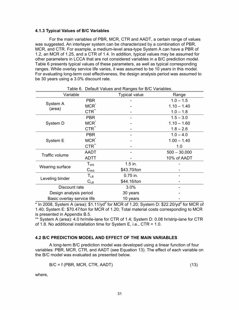
B/C variations with respect to MCR are shown in Figure 21(a) for a given range of PBR, CTR, and AADT. Compared to B/C variations with PBR as shown in Figure 20(a), B/C has a greater range of a maximum of 152%, compared to 98% in the case of PBR. This implies that PBR has more influence on B/C than MCR does. For the same PBR, CTR, and AADT, B/C variations are plotted against MCR in Figure 21(b). As the figure shows, B/C has a linear function in relation to MCR.

(a)

(b)

Figure 21. B/C variations with MCR: (a) at various PBR, CTR, and AADT; and (b) at PBR of 1.3, CTR of 1.22, and AADT of 5000.

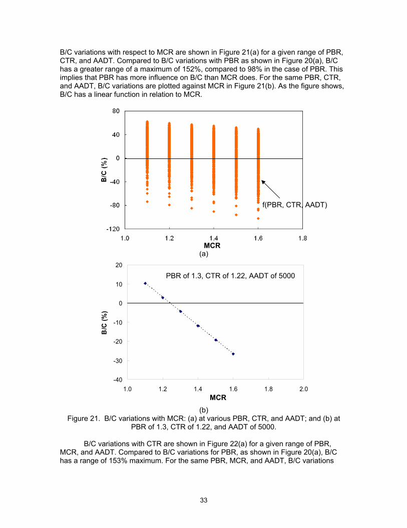
B/C variations with CTR are shown in Figure 22(a) for a given range of PBR,

MCR, and AADT. Compared to B/C variations for PBR, as shown in Figure 20(a), B/C has a range of 153% maximum. For the same PBR, MCR, and AADT, B/C variations

BRP of 1.3, TR of 1.22, AADT of 5000

-40

-30

-20

-10

0

10

20

1.0 1.2 1.4 1.6 1.8 2.0CR

B/C

(%)

f(PBR, CTR, AADT)

PBR of 1.3, CTR of 1.22, AADT of 5000

MCR

MCR

34

with CTR are plotted in Figure 21(b). As the figure shows, B/C decreases linearly with CTR.

(a)

(b)

Figure 22. B/C variations with CTR: (a) at various PBR, MCR, and AADT; and (b) at PBR of 1.4, MCR of 1.5, and AADT of 5000.

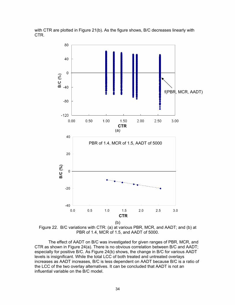
The effect of AADT on B/C was investigated for given ranges of PBR, MCR, and

CTR as shown in Figure 24(a). There is no obvious correlation between B/C and AADT; especially for positive B/C. As Figure 24(b) shows, the change in B/C for various AADT levels is insignificant. While the total LCC of both treated and untreated overlays increases as AADT increases, B/C is less dependent on AADT because B/C is a ratio of the LCC of the two overlay alternatives. It can be concluded that AADT is not an influential variable on the B/C model.

BRP of 1.4, CR of 1.5, AADT of 5000

-40

-20

0

20

40

0.0 0.5 1.0 1.5 2.0 2.5 3.0TR

B/C

(%)

f(PBR, MCR, AADT)

PBR of 1.4, MCR of 1.5, AADT of 5000

CTR

CTR

35

(a)

(b)

Figure 23. B/C variations with AADT: (a) at various PBR, MCR, and CTR; and (b) at PBR of 1.2 and 1.5, MCR of 1.2, and CTR of 1.22.

Using sensitivity analysis of potential variables, long-term B/C for 30 years is

found to be a function of PBR, MCR, and CTR. The B/C prediction model is developed through a simple linear regression using ln(PBR), MCR, and CTR as independent variables. The B/C prediction model is constructed. The analysis of variation (ANOVA) and regression results are listed in Table 7. For each variable, P-values are found to be extremely small; hence the variables are significantly important to B/C.

BRP of 1.2, CR of 1.2, TR of 1.22

BRP of 1.5, CR of 1.2, TR of 1.22

-40

-20

0

20

40

0 10 20 30 40

AADT (x1000)

B/C

(%)

f(PBR, MCR, CTR)

PBR of 1.2, MCR of 1.2, CTR of 1.22

PBR of 1.5, MCR of 1.2, CTR of 1.22

36

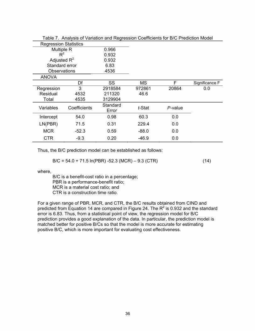
Table 7. Analysis of Variation and Regression Coefficients for B/C Prediction Model

Regression Statistics Multiple R 0.966

R2 0.932 Adjusted R2 0.932

Standard error 6.83 Observations 4536

ANOVA Df SS MS F Significance F

Regression 3 2918584 972861 20864 0.0 Residual 4532 211320 46.6

Total 4535 3129904

Variables Coefficients Standard Error t-Stat P-value

Intercept 54.0 0.98 60.3 0.0 LN(PBR) 71.5 0.31 229.4 0.0

MCR -52.3 0.59 -88.0 0.0 CTR -9.3 0.20 -46.9 0.0

Thus, the B/C prediction model can be established as follows:

B/C = 54.0 + 71.5 ln(PBR) -52.3 (MCR) – 9.3 (CTR) (14) where,

B/C is a benefit-cost ratio in a percentage; PBR is a performance-benefit ratio; MCR is a material cost ratio; and CTR is a construction time ratio.

For a given range of PBR, MCR, and CTR, the B/C results obtained from CIND and predicted from Equation 14 are compared in Figure 24. The R2 is 0.932 and the standard error is 6.83. Thus, from a statistical point of view, the regression model for B/C prediction provides a good explanation of the data. In particular, the prediction model is matched better for positive B/Cs so that the model is more accurate for estimating positive B/C, which is more important for evaluating cost effectiveness.

37

Figure 24. Comparison of obtained and predicted B/C.

4.3 MODEL VALIDATION For the medium level of material cost and construction time, two levels of model

validation were conducted to examine the proposed B/C prediction model. In the first-level validation, the B/C prediction model was validated using the PBR of interlayer systems obtained from the field. Figure 25 shows the comparison of B/C obtained from field evaluation and B/C predicted from the proposed model. Based on 19 data points, a very good correlation (R2 of 0.906 and a standard error of 7.69) is achieved in a B/C range of -33.8% to 56.7% for the three interlayer systems. Figure 26 shows the B/C difference distributions. The absolute error of the B/C is less than 10% in most cases (95%). There is only one out of the 19 locations in which the B/C difference is greater than 20%. The greatest difference in B/C—24.9%— came from the IL17 section where B/C (56.7%) and PBR (3.73) of the System E are extraordinarily high compared to the other sections.

-80

-40

0

40

80

-80 -40 0 40 80

Obtained B/C (%)

Pred

icte

d B

/C (%

)

R2 = 0.932 Standard error = 6.83 N=4535

38

Figure 25. Comparison of B/C obtained from field evaluation and from the B/C

prediction model using PBR obtained from field data.

Figure 26. B/C difference distribution in the first-level validation.

-40

-20

0

20

40

60

80

100

-40 -20 0 20 40 60 80 100Obtained B/C (%)

Pred

icte

d B

/C (%

)

System A (area)

System DSystem E

First level validation

42%

53%

0%5%

0%

20%

40%

60%

80%

100%

0 - 5 5 - 10 10 - 20 20 or more

B/C difference

R2=0.906 Standard error=7.69 n=19

39

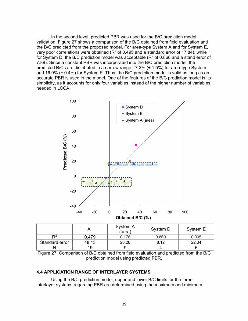
In the second level, predicted PBR was used for the B/C prediction model

validation. Figure 27 shows a comparison of the B/C obtained from field evaluation and the B/C predicted from the proposed model. For area-type System A and for System E, very poor correlations were obtained (R2 of 0.495 and a standard error of 17.84), while for System D, the B/C prediction model was acceptable (R2 of 0.868 and a stand error of 7.89). Since a constant PBR was incorporated into the B/C prediction model, the predicted B/Cs are distributed in a narrow range: -7.2% (± 1.5%) for area-type System and 16.0% (± 0.4%) for System E. Thus, the B/C prediction model is valid as long as an accurate PBR is used in the model. One of the features of the B/C prediction model is its simplicity, as it accounts for only four variables instead of the higher number of variables needed in LCCA.

All System A

(area) System D System E

R2 0.479 0.176 0.860 0.005Standard error 18.13 20.28 8.12 22.34

N 19 9 4 6 Figure 27. Comparison of B/C obtained from field evaluation and predicted from the B/C

prediction model using predicted PBR.

4.4 APPLICATION RANGE OF INTERLAYER SYSTEMS Using the B/C prediction model, upper and lower B/C limits for the three

interlayer systems regarding PBR are determined using the maximum and minimum

-40

-20

0

20

40

60

80

100

-40 -20 0 20 40 60 80 100Obtained B/C (%)

Pred

icte

d B

/C (%

)

System DSystem E

System A (area)

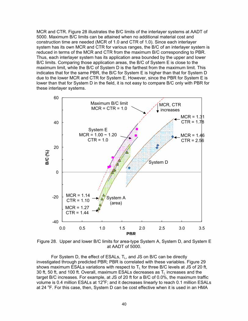
40

MCR and CTR. Figure 28 illustrates the B/C limits of the interlayer systems at AADT of 5000. Maximum B/C limits can be attained when no additional material cost and construction time are needed (MCR of 1.0 and CTR of 1.0). Since each interlayer system has its own MCR and CTR for various ranges, the B/C of an interlayer system is reduced in terms of the MCR and CTR from the maximum B/C corresponding to PBR. Thus, each interlayer system has its application area bounded by the upper and lower B/C limits. Comparing those application areas, the B/C of System E is close to the maximum limit, while the B/C of System D is the farthest from the maximum limit. This indicates that for the same PBR, the B/C for System E is higher than that for System D due to the lower MCR and CTR for System E. However, since the PBR for System E is lower than that for System D in the field, it is not easy to compare B/C only with PBR for these interlayer systems.

Figure 28. Upper and lower B/C limits for area-type System A, System D, and System E

at AADT of 5000.

For System D, the effect of ESALs, TL, and JS on B/C can be directly investigated through predicted PBR; PBR is correlated with these variables. Figure 29 shows maximum ESALs variations with respect to TL for three B/C levels at JS of 20 ft, 30 ft, 50 ft, and 100 ft. Overall, maximum ESALs decreases as TL increases and the target B/C increases. For example, at JS of 20 ft for a B/C of 0.0%, the maximum traffic volume is 0.4 million ESALs at 12oF; and it decreases linearly to reach 0.1 million ESALs at 24 oF. For this case, then, System D can be cost effective when it is used in an HMA

-40

-20

0

20

40

60

0.0 0.5 1.0 1.5 2.0 2.5 3.0 3.5

B/C

(%)

BRP

System A (area)

System D

System E MCR = 1.00 ~ 1.20

CTR = 1.0

Maximum B/C limit MCR = CTR = 1.0

MCR = 1.31 CTR = 1.78

MCR = 1.46 CTR = 2.56

MCR = 1.14 CTR = 1.10 MCR = 1.27 CTR = 1.44

MCR, CTR increases

PBR

41

overlay for which traffic volume is less than the maximum ESALs-corresponding TL: For 0.3 million ESALs, System D is cost effective at TL of 12oF; but not cost effective at TL of 20oF. At JS of 30 ft, allowable maximum ESALs become greater than that at JS of 20 ft for the considered temperature range. As joint spacing becomes greater, the allowable maximum ESALs diminish because of lower PBR for System D, despite lower MCR and CTR values. Especially, an applicable region is very limited to a low-volume (0.14 million ESALs) road at cold regions (TL of 14oF). The most cost-effective interlayer system is dependent on ESALs, TL and JS.

The expected B/C for System D can be validated using the information in Figures 29(b) and (c). Three of the four sections are within the maximum ESALs limit—US 136E (at east of San Jose), IL 267 (at Greenfield), and Mattis (at Champaign)—while the section at IL 29CC (at Creve Coeur) is beyond the maximum ESALs limit. As a result, System D proved to be a cost-effective method at the first three locations; but was found to be inefficient at IL 29CC despite the positive PBR value of 1.44.

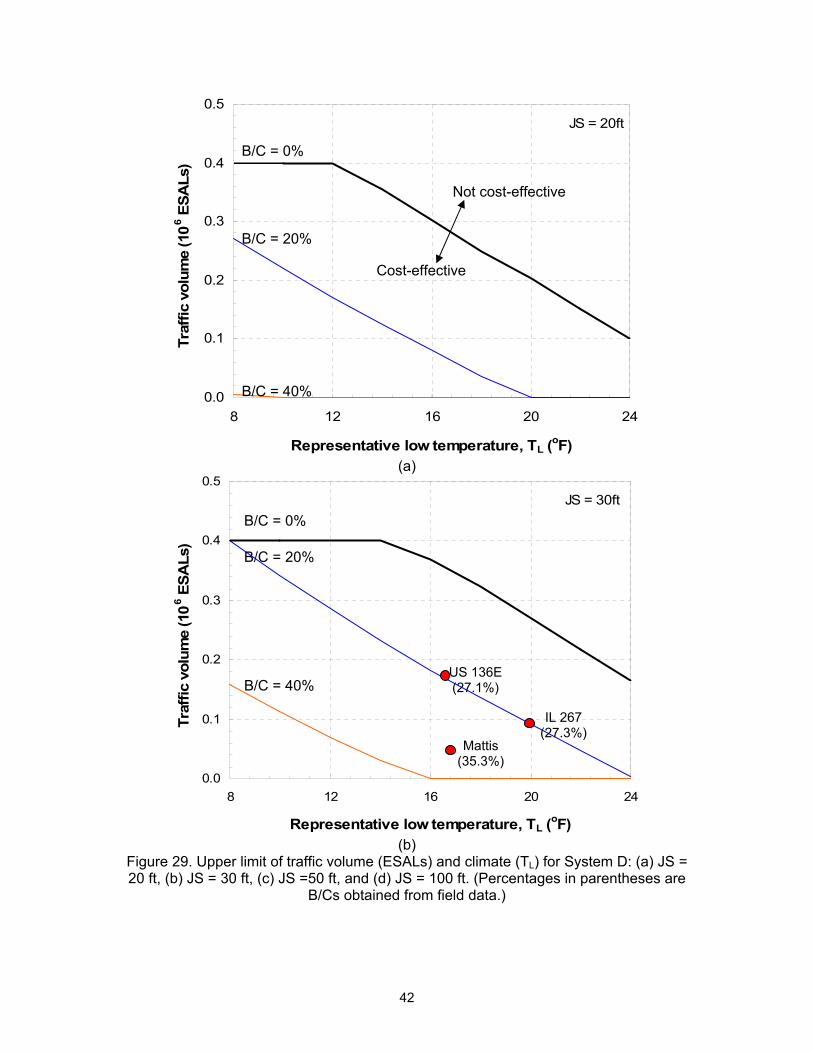
42

(a)

(b)

Figure 29. Upper limit of traffic volume (ESALs) and climate (TL) for System D: (a) JS = 20 ft, (b) JS = 30 ft, (c) JS =50 ft, and (d) JS = 100 ft. (Percentages in parentheses are

B/Cs obtained from field data.)

JS = 20ft

0.0

0.1

0.2

0.3

0.4

0.5

8 12 16 20 24

Representative low temperature, TL (oF)

Traf

fic v

olum

e (1

0 6 E

SALs

)

JS = 30ft

0.0

0.1

0.2

0.3

0.4

0.5

8 12 16 20 24

Representative low temperature, TL (oF)

Traf

fic v

olum

e (1

0 6 E

SALs

)

B/C = 0%

B/C = 20%

B/C = 40%

B/C = 40%

B/C = 20%

B/C = 0%

Mattis (35.3%)

US 136E(27.1%)

IL 267 (27.3%)

Cost-effective

Not cost-effective

43

(c)

(d)

Figure 29 (continued). Upper limit of traffic volume (ESALs) and climate (TL) for System D: (a) JS = 20 ft, (b) JS = 30 ft, (c) JS = 50 ft, and (d) JS = 100 ft. (Percentages in

parentheses are B/Cs obtained from field data.)

On the other hand, B/C for area-type System A and for System E was found to be insensitive to ESALs and TL. Based on Equation 14 with medium-level MCR and CTR

JS = 50ft

0.0

0.1

0.2

0.3

0.4

0.5

8 12 16 20 24

Representative low temperature, TL (oF)

Traf

fic v

olum

e (1

0 6 E

SALs

)

JS = 100ft

0.0

0.1

0.2

0.3

0.4

0.5

8 12 16 20 24

Representative low temperature, TL (oF)

Traf

fic v

olum

e (1

0 6 E

SALs

)

B/C = 0%

B/C = 40%

B/C = 20%

B/C = 20%

B/C = 0%

IL 29CC(-4.7%)

44

values, the average B/C of area-type System A and System E becomes -7.3% and 17.6%, respectively. Using the B/C of System E as a trigger value, the most cost-effective interlayer system can be determined with respect to ESALs and TL at various joint spacing. Figure 30 illustrates the most cost-effective interlayer system application ranges at joint spacing of 30 ft. Under the maximum ESALs limit for the B/C of 17.6%, System D is more cost effective, and System E can show better efficiency above the limit. In addition, a transition zone is established to take the uncertainty of the B/C of System E into consideration. The transition zone is bounded by upper and lower ESALs limits corresponding to B/C of 7.6% and 27.6%, respectively. Thus, the cost effectiveness of System D and System E are regarded as being comparable in the transition zone. For the application area systems, System D is relatively cost effective at low temperature with low traffic volume; System E works better at high temperature and high traffic volume. Since each district in Illinois can be represented in terms of TL, System D is generally cost effective in most northern districts and System E is ideal for southern districts.

A section at US 136 east of San Jose is the only location to use System D and System E both. Based on its ESALs (0.18 million) and TL (16.9 oF), the section lies in the transition zone. Hence, it is expected that comparable B/Cs are achieved for the two interlayer systems. As listed in Table 5, the B/C obtained is 27.1% and 31.7%, respectively, for System D and System E. This suggests that both these interlayer systems are cost effective and that their difference is marginal. This may validate the expectations obtained from the application map, but further validation is required in future studies that include ESALs and TL in B/C prediction for System E; to reduce the transition zone and to expand ESALs and TL ranges.

Figure 30. Application area for System D and System E with respect to ESALs and TL at

JS of 30 ft.

JS = 30ft

0.0

0.1

0.2

0.3

0.4

0.5

8 12 16 20 24

Representative low temperature, TL (oF)

Traf

fic v

olum

e (1

0 6 E

SALs

)

±10%

N/A

System D

System E

B/C = 17.6% (System E)

US136E

45

5. INTERLAYER SYSTEM SELECTION DECISION-MAKING

5.1 DECISION TREE FOR INTERLAYER SYSTEM SELECTION A comprehensive decision-making procedure is needed to select the most

appropriate interlayer system for an HMA overlay design. The decision tree developed considers not only cost effectiveness, but also design compatibility and the availability of interlayer systems (Figure 31). For a given HMA overlay design, three interlayer systems which have demonstrated performance benefit are provided as default alternatives. The following steps are suggested: 1. Check design compatibility with the interlayer systems. Each interlayer system has

several basic constraints. Table 8 lists the constraints associated with the three interlayer systems under investigation. Area-type System A is applicable only on a flexible base such as full-depth HMA pavement and HMA-overlaid PCC pavement (IDOT, 2002). If transverse cracks or joint spacing of PCC pavement is less than 10 ft, it is regarded as a flexible base (IDOT, 2002). Also, as a general restriction for the use of fabric interlayer systems, area-type System A is not suitable when vertical joint deflection is greater than 0.008 in and/or horizontal joint movement is greater than 2.0 in. (Button and Lytton, 2007). For System D, a 2.0-in.-thick HMA overlay is recommended as a minimum application thickness. For System E, there are no particular constraints. Consideration must also be given to which interlayer systems are currently available in a particular market.

Table 8. Interlayer System Constraints for HMA Overlays

Interlayer System Application Constraint

System A (area)

• Do not apply right over bare PCC pavements. • Do not apply if transverse cracks or joint spacing ≥ 10 ft. • Do not apply if vertical joint deflections > 0.008 in. and/or

horizontal joint movement > 0.05 in.

System D • Do not place when HMA overlay must be less than 2.0 in.

System E • N/A

2. Calculate PBR for interlayer systems to satisfy the constraints using the PBR

prediction model for System D with ESALs, TL, and JS; or by using the average PBR of 1.22 and 1.49 for area-type System A and for System E. Interlayer systems whose PBR is less than 1.0 are discarded because there is no possibility of them being cost-effective.

3. Evaluate the cost effectiveness of the interlayer systems to select the most cost-effective based on the level of project importance and data availability. Unless information on specific interlayer systems and HMA overlay is available, the most cost-effective interlayer system can be simply determined based on the information in Figures 29 and 30 (Level I), assuming that a medium cost level interlayer system and an HMA overlay system is used.

4. The optimal interlayer system is determined using ESALs, TL, and JS. If ESALs, TL, and JS are out of the ranges provided in the Figure 29 and Figure 30 and/or a

46

specific material cost and construction time can be known, the B/C prediction model (see Equation. 14) can be used to achieve the B/C for each interlayer system (Level II). However, since the B/C prediction model was developed using a discount rate of 3.0%, the model may not be valid for other discount rates. If the calculated B/C of an interlayer system is between -10% and 10%, a more accurate B/C calculation is suggested because the B/C prediction model standard error is 6.8%.

5. CIND may be used to obtain the most accurate B/C for interlayer systems (Level III), which requires detailed characteristics of the interlayer systems, overlays, and other variables related to LCCA.

6. By comparing the B/C values of alternative interlayer systems, the most cost-effective interlayer system can be determined.

47

Figure 31. Decision tree for selecting a cost-effective interlayer system for HMA overlay.

Alternative Interlayer Systems

I. System A (area) II. System D (strip) III. System E (area)

• Eq. 1 • ESALs, TL, JS

HMA Overlay Design

Overlay Thickness Existing Pavement Traffic & Location

• Overlay Structure • Market Feasibility

Cost-Effectiveness Evaluation

Yes

No Yes

Satisfy Constraints?

No

PBR >1

MCR, CTR?

Discard

Yes

Cost-effective interlayer system

selection

B/C

B/C (CIND)

>10%

<-10% [-10%, 10%]

Figure 29 and 30 (ESALs, TL, JS) i = 3.0% No

Yes

B/C (Eq. 14)

No

III

II

I

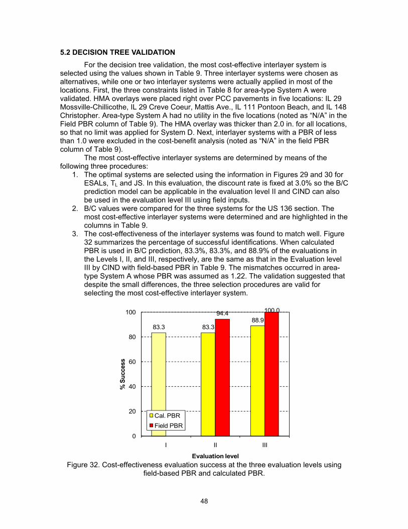
48

5.2 DECISION TREE VALIDATION For the decision tree validation, the most cost-effective interlayer system is

selected using the values shown in Table 9. Three interlayer systems were chosen as alternatives, while one or two interlayer systems were actually applied in most of the locations. First, the three constraints listed in Table 8 for area-type System A were validated. HMA overlays were placed right over PCC pavements in five locations: IL 29 Mossville-Chillicothe, IL 29 Creve Coeur, Mattis Ave., IL 111 Pontoon Beach, and IL 148 Christopher. Area-type System A had no utility in the five locations (noted as “N/A” in the Field PBR column of Table 9). The HMA overlay was thicker than 2.0 in. for all locations, so that no limit was applied for System D. Next, interlayer systems with a PBR of less than 1.0 were excluded in the cost-benefit analysis (noted as “N/A” in the field PBR column of Table 9).

The most cost-effective interlayer systems are determined by means of the following three procedures:

1. The optimal systems are selected using the information in Figures 29 and 30 for ESALs, TL and JS. In this evaluation, the discount rate is fixed at 3.0% so the B/C prediction model can be applicable in the evaluation level II and CIND can also be used in the evaluation level III using field inputs.

2. B/C values were compared for the three systems for the US 136 section. The most cost-effective interlayer systems were determined and are highlighted in the columns in Table 9.

3. The cost-effectiveness of the interlayer systems was found to match well. Figure 32 summarizes the percentage of successful identifications. When calculated PBR is used in B/C prediction, 83.3%, 83.3%, and 88.9% of the evaluations in the Levels I, II, and III, respectively, are the same as that in the Evaluation level III by CIND with field-based PBR in Table 9. The mismatches occurred in area-type System A whose PBR was assumed as 1.22. The validation suggested that despite the small differences, the three selection procedures are valid for selecting the most cost-effective interlayer system.

Figure 32. Cost-effectiveness evaluation success at the three evaluation levels using

field-based PBR and calculated PBR.

83.3 83.388.9

94.4 100.0

0

20

40

60

80

100

I II III

% S

ucce

ss

Evaluation level

Cal. PBRField PBR

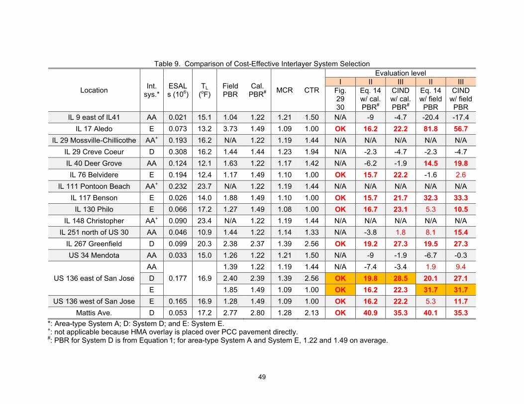
49

Table 9. Comparison of Cost-Effective Interlayer System Selection

Location Int. sys.*

ESALs (106)

TL (oF)

Field PBR

Cal. PBR# MCR CTR

Evaluation level I II III II III

Fig. 29 30

Eq. 14 w/ cal. PBR#

CIND w/ cal. PBR#

Eq. 14 w/ field PBR

CIND w/ field PBR

IL 9 east of IL41 AA 0.021 15.1 1.04 1.22 1.21 1.50 N/A -9 -4.7 -20.4 -17.4 IL 17 Aledo E 0.073 13.2 3.73 1.49 1.09 1.00 OK 16.2 22.2 81.8 56.7

IL 29 Mossville-Chillicothe AA+ 0.193 16.2 N/A 1.22 1.19 1.44 N/A N/A N/A N/A N/A IL 29 Creve Coeur D 0.308 16.2 1.44 1.44 1.23 1.94 N/A -2.3 -4.7 -2.3 -4.7 IL 40 Deer Grove AA 0.124 12.1 1.63 1.22 1.17 1.42 N/A -6.2 -1.9 14.5 19.8 IL 76 Belvidere E 0.194 12.4 1.17 1.49 1.10 1.00 OK 15.7 22.2 -1.6 2.6

IL 111 Pontoon Beach AA+ 0.232 23.7 N/A 1.22 1.19 1.44 N/A N/A N/A N/A N/A IL 117 Benson E 0.026 14.0 1.88 1.49 1.10 1.00 OK 15.7 21.7 32.3 33.3

IL 130 Philo E 0.066 17.2 1.27 1.49 1.08 1.00 OK 16.7 23.1 5.3 10.5 IL 148 Christopher AA+ 0.090 23.4 N/A 1.22 1.19 1.44 N/A N/A N/A N/A N/A

IL 251 north of US 30 AA 0.046 10.9 1.44 1.22 1.14 1.33 N/A -3.8 1.8 8.1 15.4 IL 267 Greenfield D 0.099 20.3 2.38 2.37 1.39 2.56 OK 19.2 27.3 19.5 27.3 US 34 Mendota AA 0.033 15.0 1.26 1.22 1.21 1.50 N/A -9 -1.9 -6.7 -0.3

US 136 east of San Jose AA

0.177 16.9 1.39 1.22 1.19 1.44 N/A -7.4 -3.4 1.9 9.4

D 2.40 2.39 1.39 2.56 OK 19.8 28.5 20.1 27.1 E 1.85 1.49 1.09 1.00 OK 16.2 22.3 31.7 31.7

US 136 west of San Jose E 0.165 16.9 1.28 1.49 1.09 1.00 OK 16.2 22.2 5.3 11.7 Mattis Ave. D 0.053 17.2 2.77 2.80 1.28 2.13 OK 40.9 35.3 40.1 35.3

*: Area-type System A; D: System D; and E: System E. +: not applicable because HMA overlay is placed over PCC pavement directly. #: PBR for System D is from Equation 1; for area-type System A and System E, 1.22 and 1.49 on average.

50

6. CONCLUSIONS AND RECOMMENDATIONS

6.1 SUMMARYLife-cycle cost analysis (LCCA) was conducted to assess the engineering value

of interlayer systems used in Illinois to control reflective cracking. Cost effectiveness was evaluated by means of a benefit-cost ratio (B/C) obtained through LCCA. A user-friendly LCCA spreadsheet-based program was developed called Cost-effective INterlayer system Decision (CIND). Field performance data, material costs, and construction procedures were used to develop a regression model to predict the B/C of the interlayer systems. Using this model, a schematic illustrating cost-effective regimes for the employment of interlayer systems was developed as a function of traffic volume and climatic region within Illinois. From this, a decision tree was constructed to aid the designer in the selection of a cost-effective and compatible interlayer system for a given pre-existing pavement system.

Of the five interlayer systems evaluated in the companion report, Volume I (Al-Qadi et al. 2008) conducted in Illinois, three interlayer systems with positive performance-benefit ratio were investigated: area-wide System A (a nonwoven polypropylene geotextile fabric); System D (an interlayer stress-absorbing composite [ISAC] strip treatment); and System E (a sand-sized aggregate gradation with high binder content and a highly modified binder).

Based on the research, the following conclusions have been made:

• Based on a statistical analysis of the B/C prediction model’s ability to predict field

performance data, the model was found to be effective for estimating the B/C of interlayer systems over a 30-year analysis period using just three variables: performance-benefit ratio (PBR), material cost ratio (MCR), and construction time ratio (CTR).

• Based on 19 interlayer systems evaluated in the field, the B/C of area-type System A ranged from -29.4% to 16.0%; while Systems D and E carried B/C ratios of -9.7% to 28.5% and 4.0% to 59.8%, respectively. Strip applications involving Systems A and B were found to have negative B/C, due to their poor performance in terms of abating reflective cracking as measured in field surveys.

• The effects of PBR, MCR, and CTR on the benefit versus cost of interlayer systems were clearly demonstrated. B/C increases linearly as ln(PBR) increases; but decreases linearly as MCR and CTR increase.

• Among the three interlayer systems, System D has the widest application range in terms of ESALs, TL, and JS, especially in colder regions in Illinois with lower traffic volume. On the other hand, System E is cost effective in warmer regions with higher traffic volume. As joint spacing increases, the application range of System D is diminished. Area-type System A exhibited a marginal cost effectiveness only in limited survey locations.

6.2 EXPECTED BENEFITS This study developed a decision-making procedure for selecting a cost-effective

interlayer system in the State of Illinois when HMA overlay is used for pavement rehabilitation. A simple decision tree was developed, based on comprehensive analyses conducted using an LCCA program, a B/C prediction model, and application range tables developed in this study. For convenience, a chart method was developed to guide

51

the designer in interlayer system selection with respect to equivalent single-axle loads (ESALs), representative low temperature (TL) in the design location in Illinois, and PCC pavement joint spacing (JS). Local agencies and/or pavement engineers can use one or more of these decision-making tools, which range in complexity based on project size and/or importance. Using this adaptive approach is expected to save significant cost and time and to produce more predictable performance outcomes when using reflective crack control treatments in conjunction with HMA overlays in Illinois.

6.3 RECOMMENDATIONS

• The accuracy of the LCCA program and CIND mainly depends on the performance-benefit ratio of interlayer systems. Using reliable input variables into the LCCA program and CIND are recommended for selecting cost-effective interlayer systems for larger, high-profile rehabilitation projects. For the purpose of preselection or lower-profile projects, the B/C prediction model and/or application tables are recommended for use.

• More data and efforts are needed to fine-tune the B/C prediction model which is only valid for low traffic volume roads, not for interstate. This can be accomplished by surveying additional sections and/or by obtaining more data from previously surveyed sections.

52

7. REFERENCES Al-Qadi, I. L., W. G. Buttlar, J. Baek, and M. Kim (2008). Cost Effectiveness and

Performance of Overlay Systems in Illinois-Volume I: In-Situ Assessment of Interlayer Systems Used in Illinois. Final Report, Illinois Center for Transportation, Illinois Department of Transportation, Springfield.

Beg, M. A., Z. Zhang, and W. R. Hudson (2000). Development of Pavement Type Evaluation Procedure for Texas Department of Transportation, Transportation Research Record: Journal of the Transportation Research Board, No. 1699, Transportation Research Board of the National Academies, Washington, D.C., pp. 23–32.

Buttlar, W. G., B. Diyar, and B. Dempsey (1999). Evaluation of Reflective Crack Control Policy, Report No. ITRC FR 95/96-4, Illinois Transportation Research Center, University of Illinois at Urbana-Champaign, Urbana.

Buttlar, W. G., B. Diyar, and B. Dempsey (2000). Cost-Effectiveness of Paving Fabric Used to Control Reflective Cracking, Transportation Research Record: Journal of the Transportation Research Board, No. 1730, Transportation Research Board of the National Academies, Washington, D.C., pp. 139–149.

Button, J. W. and R. L. Lytton (2007). Guidelines for Using Geosynthetics with Hot Mix Asphalt Overlays to Reduce Reflective Cracking. Presented at 86th Annual Meeting of the Transportation Research Board, Washington, D.C.

Federal Highway Administration, (1998). Life Cycle Cost Analysis in Pavement Design. Publication FHWA-SA-98-400, U.S. Department of Transportation.

Geoffrey, D. N. (1996). Cost-Effective Preventive Pavement Maintenance.. NCHRP Synthesis 223, Transportation Research Board, Washington, D.C.

IDOT, (2002). Bureau of Design and Environment Manual, Illinois Department of Transportation, Springfield.

Lamptey, G., M. Ahmad, S. Labi, and K. Sinha (2005). Life Cycle Cost Analysis for INDOT Pavement Design Procedures. Publication FHWA-IN-JTRP-2004-28, Purdue University, West Lafayette, Ind.

NCHRP (2003). NCHRP 2002 Design Guide – Pavement Analysis and Design System, NCHRP 1-37a. ERES Division of Applied Research Associates and Arizona State University, Tempe.

U.S. Department of Labor. Consumer Price Index. http://www.bls.gov/CPI/. Accessed May 1st, 2008.

Vespa, J. W. (2005). An Evaluation of Interlayer Stress Absorbing Composite Reflective Crack Relief System. Publication FHWA-IL-PRR-150, Illinois Department of Transportation, Springfield.

Wei, C. and S. Tighe (2004). Development of Preventive Maintenance Decision Trees Based on Cost-Effectiveness Analysis, Transportation Research Record: Journal of the Transportation Research Board, No. 1866, Transportation Research Board of the National Academies, Washington, D.C., pp. 9–19.

A-1

APPENDIX A

User Manual for CIND Version 1.0

LifeCost

e-Cycle Cot-Effective

ost AnalyInterlayer

Illinois

Illino

ysis Progr System D

CVe

Use

Dece

s Departm

ois Cente

A-2

gram: Decision fo

CINDersion 1.0

er Manua

ember 200

ment of Tra

er for Tran

or Hot-Mix A

al

08

ansportat

nsportation

Asphalt Ov

ion

n

verlay

A-3

Acknowledgements Technical review panel members of ICT-RC58 Project, Cost-Effectiveness and Performance of Overlay Systems in Illinois are Joseph Vespa (Chair), Amy Schutzbach, David Lippert, James Trepanier, Aaron T. Toliver, and Patricia Broers

A-4

A.1 INTRODUCTION Interlayer systems are used in hot-mix asphalt (HMA) overlays to retard reflective cracking. Among various alternatives, a cost-effective interlayer system is determined through a life-cycle cost analysis (LCCA). Based on the performance benefit of interlayer systems to control reflective cracking, the relative cost benefit of interlayer systems is computed as a benefit-cost ratio (B/C) using a cost-effective interlayer system decision program (CIND). The program is coded with Microsoft Excel Visual Basic for Application (VBA). In CIND, the LCCA procedure suggested by the Federal Highway Administration (FHWA, 1998) is adapted and the same approach of RealCost Version 2.2 (FHWA, 2004) is used to compute user costs. Furthermore, the LCCA procedure is modified appropriately for HMA overlays. A.2 CIND DESCRIPTION A.2.1 CIND Framework CIND consists of three main modules shown in Figure A.1: Input, Analysis, and Output. In the input module, all input variables are given for HMA overlay, interlayer systems, traffic, and LCCA parameters. Users enter information for major parameters for overlay geometry, interlayer type, and traffic; minor or unfamiliar parameters are provided as default values by the program. In particular, performance-benefit ratio is also provided as a default value. During LCCA analysis, agency and user costs are computed based on user’s input variables and default values. Finally, the LCCA results are presented in the output modules as a summary report, as well as graphs for each cost component. The most cost-efficient interlayer system is computed based on the relative B/C.

Figure A.1. Framework for the cost-effective interlayer selection decision program

(CIND).

Input

HMA Overlay

Interlayer

Traffic

Analysis

Agency Cost

User Delay Cost

Output

Grand Total Cost

Cost-Effective Interlayer System

Evaluation

Material price Construction period Lane configurations

Material price Construction period

Service life

AADT

Overlay cost Interlayer cost Salvage value

Free flow cost Forced cost

Salvage value Default values

Agency cost User delay cost

Net present value

LCCA Parameters

Performance- benefit ratio

A-5

A.2.2 Starting CIND Under a medium security level in Excel 2003 or other versions, security warning options are shown (Figure A.2) whenever CIND starts. To run CIND, the “Enable Macros” option should be chosen.

Figure A.2. Microsoft Excel 2003 macro options form

When CIND opens correctly, a CIND startup form appears as the “main” worksheet as shown in Figure A.3.

Figure A.3. CIND startup form

After clicking the startup form or the “Click to Start” button, the main menu appears (Figure A.4). The main menu contains six items as follows:

- Design Input: All data for pavement structure, costs, traffic, and performance are entered via an input form.

- LCCA Output: LCCA analysis outputs are shown with five charts for agency, user, total, and accumulated costs, and B/C.

A-6

- View Report: Users can modify design input directly in a “Report” worksheet; moreover, a new LCCA can be run.

- Print Report: The summary report can be printed out. - Export Data: Data can be stored in a separate file which can be imported later.

The export data is saved in the same directory where CIND is working.

- Exit: Terminate the CIND and return to a “Main” worksheet.

Figure A.4. Main menu in CIND

A.2.3 Design Input Variables A.2.3.1 Input option There are three input method options: Direct Input for New Data; Update Existing Data; and Import New Data (see Figure A.5). When users create new design input data, previous data is deleted and all design variables are initialized accordingly. Once input data are imported or modified by users in a “Report” worksheet, the data can be updated by selecting “Update Existing Data.” The last input option can be chosen when input data files have already been generated.

A-7

Figure A.5. Data input option form

The design input has four categories for overlay, interlayer system, traffic, and LCCA parameters as follows:

- Overlay Project identification, geometry, and HMA overlay information are given.

- Interlayer system: Alternative interlayer systems and details for material price and installation period are given.

- Traffic: Road category, work zone, and annual average daily traffic (AADT) are given when user costs are included.

- LCCA: Design year and performance-benefit ratio are given. A.2.3.2 Overlay Figure A.6 shows the input form to be filled in to identify project, specify overlay geometry, and identify costs for materials and construction . Overlay input variables and their descriptions are listed in Table A.1. In each design input form, users can bring up a table for design variables through the “Help” button. The next step is activated by pressing the “Next” button. If necessary data are missing, an error message is shown and the user is returned to the overlay design input form. Users can click the “Back” button to return to the input option.

A-8

Figure A.6. Project identification and overlay information input form

Table A.1. Overlay Input form Variables

Category Option/Input Description

Geometry

Lane length Total project lane length or evaluation length (miles)

Lane width Default value of 12 ft regardless of inner or outer lane

Number of lanes Number of lanes in each direction, up to 3

Joint spacing Longitudinal slab span length of pre-existing concrete pavements, ranging from10 to 100ft

HMA overlay

Thickness Thickness of wearing surface and leveling binder (in.)

Material Material price ($/ton)

Construction Additional construction cost if needed ($/in-lane-mile)

Period Construction period (hr/in-lane-mile)

A-9

A.2.3.3 Interlayer system Figure A.7 shows the CIND interlayer system variable input form. In this form, four types of interlayer system alternatives are provided; only three interlayer systems having positive performance-benefit ratio can be available to choose: System A (area-type), System D, and System E. General information appears when an interlayer system name is clicked (see Figure A.8). When a box next to the name is checked, the interlayer system is selected and then the second input tab is activated. Type, product, and unit price of the interlayer system material and installation are entered accordingly. Unless the desired product is found in the product list, “User-defined” is selected and a specific product name and unit price are entered in a pop-up input box. According to the selected product, unit price is provided as a default, but also can be entered manually. When installation information is not available, users can use default values as given; specific unit price, width and number of strips, as well as installation period. This can be repeated until all information is correctly entered. Detailed input variables are listed in Table A.2. The next step is activated by pressing the “OK” button. If necessary data are missing, an error message will appear as shown in Figure A.9 and the user is guided to the input form.

Figure A.7. Interlayer system variables input form

A-10

Figure A.8. General information for four interlayer systems

Figure A.9. Warning message for input error

(a) (b)

(c) (d)

A-11

Table A.2. Interlayer System Input Variables Category Option/Input Description

Interlayer system

Type System A: area System D: strip System E: area

Product name Currently used product

Product unit price Systems A and D: $/yd2

System E: $/ton

Installation unit price

Additional price to install interlayer systems Strip type: $/strip (System D) Area type: $/lane-mile (System A) $/in-lane-mile (System E)

Width Width of strip type interlayers (ft)

Number of strips Same as the number of joints or actual number of strips used

Installation day

Additional time to install interlayer system Strip type: hr/strip (System D) Area type: hr/lane-mile (System A) hr/in-lane-mile (System E)

A-12

A.2.3.4 Traffic User cost is calculated based mainly on traffic volume of a road as well as geometry. A box is checked to include the user cost. Otherwise, only agency cost is considered to evaluate the cost benefit of interlayer systems. Figure A.10 shows a traffic input form. Detail input variables are listed in Table A.3. In order to determine hourly traffic distribution, it needs to determine the category and priority of a road: Urban or Rural; and interstate, principal arterial, and minor arterial. Interstate highways are not incorporated in this program since the performance-benefit ratio of the interstate highways is not included. Traffic volume is given based on a current (construction) year by means of annual average daily traffic (AADT), which is divided into three classes: passenger cars, single-unit trucks, and multiple-unit trucks to include all other trucks. Annual ESALs in a design lane is calculated base on the traffic volume and road class. If the class of a design road is known, this should be selected. Otherwise, “N/A” can be chosen; it will then be determined from number of lanes and AADT. The growth rate of the traffic volume is given; it is uniform to the three classes of vehicles. Work zone capacity is computed based on lane opening, speed change, and length of the work zone area, as well as period of work zone in effect.

Figure A.10. Traffic parameters input form

A-13

Table A.3. Traffic Input Variables

Category Option/Input Description

Traffic

Category Urban or rural

Priority Principal arterial and minor arterial

Current Year First year of the analysis period used as base year of an expenditure diagram

AADT Annual average daily traffic in both directions in current year

Road Class

Illinois road classifications regarding traffic volume and number of lanes (1: more than 4 lanes, 2: AADT >= 1000, 3: AADT >= 400, 4 AADT < 400

Growth Rate Annual traffic growth rate of AADT (same rate for all vehicles)

Passenger Cars % of passenger car in AADT

Single-Unit Trucks % of single-unit trucks in AADT

All Other Trucks % of combination trucks in AADT

Work zone

Lane Opening in Work Zone

Number of lanes open in work zone area in each direction, up to two lanes

Upstream Speed Speed limit in normal operation (mph)

Work Zone Speed Speed limit in work zone area (mph)

Work Zone Length Maximum length of work zone area when vehicle speed is reduced (miles)

Work Zone Duration Duration for work zone in effect; (“all day” option used as default)

A-14

A.2.3.5 LCCA A life-cycle cost analysis is executed with the parameters shown in Table A.4 to define a service life span for each overlay design. Figure A.11 shows an LCCA input form. For an analysis period, multiple overlays are considered corresponding to the service life of overlays. Future cost is converted to a current value via a discount rate, and a net present value (NPV) is computed to sum all agency and user costs in initial and consecutive sequences during the analysis period. To compensate for a remaining life of the last overlay, a salvage value is determined at the end of the analysis period. The most important parameter of the LCCA is a performance-benefit ratio of interlayer systems. The benefit ratio, PBR, is a ratio of deteriorated rate of an overlay to an overlay with an interlayer system as follows:

systemterlayerinanwithoutoverlayHMAanofspanlifeServicesystemterlayerinanwithoverlayHMAanofspanlifeServiceBRP = (A.1)

Figure A.11. LCCA parameters input form

A higher benefit ratio indicates a longer service life for the overlay section with an interlayer system compared to the control. The benefit ratio of a specific interlayer system is a default value in the program, based on a companion research report (Al-Qadi et al., 2008). If users have their own source for the benefit ratio, it can be substituted. Care must be exercised as this value has a significant effect on the LCCA, so a warning message pops up when the default benefit ratios are to be changed (see

A-15

Figure A.12). With the exception of the parameters given in Table A.4, all other parameters required for the LCCA are default values in the program; such as value of travel time (11.58$/veh-hr for passenger cars, 18.54$/veh-hr for single-unit trucks, and 22.31$/veh-hr for other trucks). These values reflect adjusted dollar values in terms of the 1996 base year, using an inflation rate calculated based on the U.S. consumer price index (U.S. Department of Labor, 2008). Detailed values for the LCCA are shown in an “intermediate results” worksheet. Finally, a “Run LCCA” button at the end of the LCCA part of the program executes the LCCA ; the results are shown in a form.

Figure A.12 Warning message to alert to change in default values

Table A.4. LCCA Input Variables

Category Option/Input Description

Service life parameters

Analysis period Total number of years to be analyzed, up to 50 years

Overlay service life Overlay service life span with no interlayer system (years)

Discount rate Rate to convert future cost to present value (3% to 5%)

Interlayer systems Benefit ratio

Ratio to extend service life of overlay with interlayer systems compared to untreated overlay

A-16

A.2.4 LCCA Results In the LCCA output module, LCCA results are shown in a chart form: for the first overlay service life span, agency and user costs; and for the entire analysis period, total cost as equivalent uniform annual cost (EUAC), B/C, and accumulated cost. A.2.4.1 Agency cost Agency cost is comprised of basic construction cost for the HMA overlay, additional cost for interlayer systems, and a salvage value. For the first overlay service life span corresponding to the control section, the salvage value is negative if the performance-benefit ratio of an interlayer system is greater than 1.0, which reduces the total agency cost of the interlayer system. In the example shown in Figure A.13, all interlayer systems have positive salvage values because their PBRs are greater than 1.0. Total agency cost of an alternative design becomes higher than that of the control section when an additional cost is higher than the salvage value.

Figure A.13. Agency cost result form

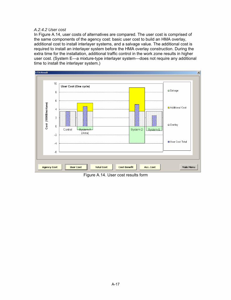
A-17

A.2.4.2 User cost In Figure A.14, user costs of alternatives are compared. The user cost is comprised of the same components of the agency cost: basic user cost to build an HMA overlay, additional cost to install interlayer systems, and a salvage value. The additional cost is required to install an interlayer system before the HMA overlay construction. During the extra time for the installation, additional traffic control in the work zone results in higher user cost. (System E—a mixture-type interlayer system—does not require any additional time to install the interlayer system.)

Figure A.14. User cost results form

A-18

A.2.4.3 Total cost Instead of net present value, an equivalent uniform annual cost (EUAC) is computed to compare total cost for the HMA overlay life cycle. The EUACs for the various alternative designs are shown in Figure A.15. The alternative design, whose EUAC is lower than that of the control section, has a positive B/C. In addition, the ratio of the agency cost to user cost implies which of these is more important for the selection of an interlayer system for a given project. Figure A.15 is a good example demonstrating that user cost does not have a major impact on LCCA because of its relatively low contribution compared to the agency cost, regardless of the interlayer systems.

Figure A.15. Total cost results form

A-19

A.2.4.4 Cost benefit Using the EUAC for alternative HMA overlay sections, B/C of the alternatives is calculated and compared to that of the control section. Figure A.16 shows the B/C of the alternatives. System E has the highest B/C among the interlayer systems. The cost benefit result is shown in a pop-up window (see Figure A.17(a) or A.17(b)). Also, the LCCA input and output can be verified in a “Report” worksheet.

Figure A.16. Cost benefit results form

(a)

(b)

Figure A.17. Cost benefit result of the alternatives when (a) there is a cost-effective interlayer system and (b) there is no cost-effective system.

A-20

A.2.4.5 Accumulated cost Figure A.18 shows that the total costs for the HMA overlay construction and user delay are accumulated. In this figure, the control section requires six overlays over the analysis period while overlay design with System D requires only three overlays. However, the cost of System D for one-time overlay construction is higher than that of the control section. System E requires a comparable cost each time; but less frequent constructions. Hence, it shows the best cost benefit.

Figure A.18. Accumulated costs form for the analysis period

A.2.5 Report The last command in the main menu is “Print Report” to print a brief report on the LCCA input and output. As shown in Figure A.19, the report contains all entered data in the design module, charts shown in the LCCA output, NPVs, EUACs, and B/C for the alternative designs.

A-21

Figure A.19. Sample brief report

1. Project Information

Project No. 12345District 4County Country

City CityDescription Description

Lane Length 1 miLane Width 12 ft

Number of Lanes 1 in each directionJoint Spacing 30 ft

Wearing surfaceThickness 1.50 in

Material Unit Price 40.0 $/tonConstruction cost 0.0 $/in-lane-mileConstruction Time 4 hr/in-lane-mile

Leveling binderThickness 0.75 in

Material Unit Price 40.0 $/tonConstruction cost 0.0 $/in-lane-mileConstruction Time 4 hr/in-lane-mile

2. Interlayer System Alternatives

Type Area Type StripManufacturer Petromat Manufacturer ISAC

Unit Price 0.45 $/sq.yd Unit Price 21.51 $/sq.ydWidth N/A Width 3 ft

Number of Strips N/A Number of Strips 352Intallation Price 0 $/lane-mile Intallation Price 0 $/strip

Delay Time 5 hr/lane-mile Delay Time 0.08 hr/strip

Type Type AreaManufacturer Manufacturer IL4.95mm

Unit Price $/sq.yd Unit Price 46.2 $/ tonWidth ft Width N/A

Number of Strips Number of Strips N/AIntallation Price $/strip Intallation Price 0 $/lane-mile

Delay Time hr/strip Delay Time 0 hr/lane-mile

3. Traffic Information

Category RuralPrincipal Arterial Class 2

Traffic volum Current Year 2000AADT 5000 ESAL 623

Vehicle Passinger Cars 80 % Growth rate 3 %Single-Unit Trucks 10 %

Combination Trucks 10 %Work zone Lane Opening 1

Upstream Speed 55 mphWork Zone Speed 20 mphWork Zone Length 1 mile

Work Zone Duration All day

4. Life-Cycle Cost Analysis Input

Parameter Overlay service life 6 years Design year 35 yearsDiscount rate 3 %

Benefit ratio System A Area Petromat 1.22

System D

System E

Life-Cycle Cost Analysis Report on Project #12345

Alternative 1

Alternative 2

Alternative 3

Location

Geometry

Overlay

Alternative 4

System A

System B

A-22

A.3 REFERENCES 1. Federal Highway Administration (1998), Life-Cycle Cost Analysis in Pavement

Design, Report FHWA-SA-98-079, U.S. Department of Transportation. 2. Federal Highway Administration (2004), Life-Cycle Cost Analysis: RealCost, User

Manual, Office of Asset Management, FHWA, U.S. Department of Transportation. 3. U.S. Department of Labor (2008), Consumer Price Index. http://www.bls.gov/CPI/

Accessed on May 1, 2008. 4. Al-Qadi, I. L., W. G. Buttlar, J. Baek, and M. Kim (2008), Cost Effectiveness and

Performance of Overlay Systems in Illinois – Volume 1: Effectiveness Assessment of HMA Overlay Interlayer System Used to Retard Reflective Cracking, Report FHWA-ICT-00-000, Illinois Center for Transportation, Illinois Department of Transportation, Springfield, IL.

B-1

APPENDIX B

Table B.1 Elevation Factors for Each Category Table B.2 LCCA Result for Area-Type System A Table B.3 LCCA Result for System D Table B.4 LCCA Result for System E Table B.5. Material Cost Corresponding to MCR

B-2

B.1 Elevation Factors for Each Category

Year Elevation Factor Traffic System A System B System D System E

1984 0.660 0.600 0.489 0.489 0.559 1985 0.690 0.627 0.511 0.511 0.585 1986 0.700 0.636 0.519 0.519 0.593 1987 0.720 0.655 0.533 0.533 0.610 1988 0.750 0.682 0.556 0.556 0.636 1989 0.790 0.718 0.585 0.585 0.669 1990 0.830 0.755 0.615 0.615 0.703 1991 0.870 0.791 0.644 0.644 0.737 1992 0.890 0.809 0.659 0.659 0.754 1993 0.920 0.836 0.681 0.681 0.780 1994 0.940 0.855 0.696 0.696 0.797 1995 0.970 0.882 0.719 0.719 0.822 1996 1.000 0.909 0.741 0.741 0.847 1997 1.020 0.927 0.756 0.756 0.864 1998 1.040 0.945 0.770 0.770 0.881 1999 1.060 0.964 0.785 0.785 0.898 2000 1.100 1.000 0.815 0.815 0.932 2001 1.130 1.027 0.837 0.837 0.958 2002 1.150 1.045 0.852 0.852 0.975 2003 1.180 1.073 0.874 0.874 1.000 2004 1.200 1.091 0.889 0.889 1.017 2005 1.240 1.127 0.919 0.919 1.051 2006 1.280 1.164 0.948 0.948 1.085 2007 1.320 1.200 0.978 0.978 1.119 2008 1.350 1.227 1.000 1.000 1.144

B-3

Table B.2 LCCA Result for Area-Type System A US34

Mendota PBR Construction Service life (year) Analysis period (year) 1.26 1997 11 11

Material cost (unit price) EUAC (1000$/mi-lane)

Sys. A (area)

Cost level

Wearing surface ($/ton)

Leveling binder ($/ton) MCR Agency User Total B/C (%)

H

33.02 33.37

1.31 7.27 0.16 7.43 -7.04 M 1.21 6.80 0.16 6.96 -0.32 L 1.16 6.57 0.16 6.73 3.04

Control - 6.81 0.13 6.94 0.00 IL40

Deer Grove PBR Construction Service life (year) Analysis period (year) 1.63 1998 10 10

Material cost (unit price) EUAC (1000$/mi-lane)

Sys. A (area)

Cost level

Wearing surface ($/ton)

Leveling binder ($/ton) MCR Agency User Total B/C (%)

H

33.67 34.02

1.25 6.73 0.19 6.92 10.37 M 1.17 6.29 0.19 6.48 16.01 L 1.13 6.08 0.19 6.27 18.75

Control - 7.53 0.19 7.72 0.00 IL251

North of US30 PBR Construction Service life (year) Analysis period (year) 1.44 1995 13 13

Material cost (unit price) EUAC (1000$/mi-lane)

Sys. A (area)

Cost level

Wearing surface ($/ton)

Leveling binder ($/ton) MCR Agency User Total B/C (%)

H

31.40 31.73

1.20 6.69 0.09 6.78 4.54 M 1.14 6.33 0.09 6.42 9.56 L 1.11 6.15 0.09 6.24 12.07

Control - 7.02 0.09 7.10 0.00

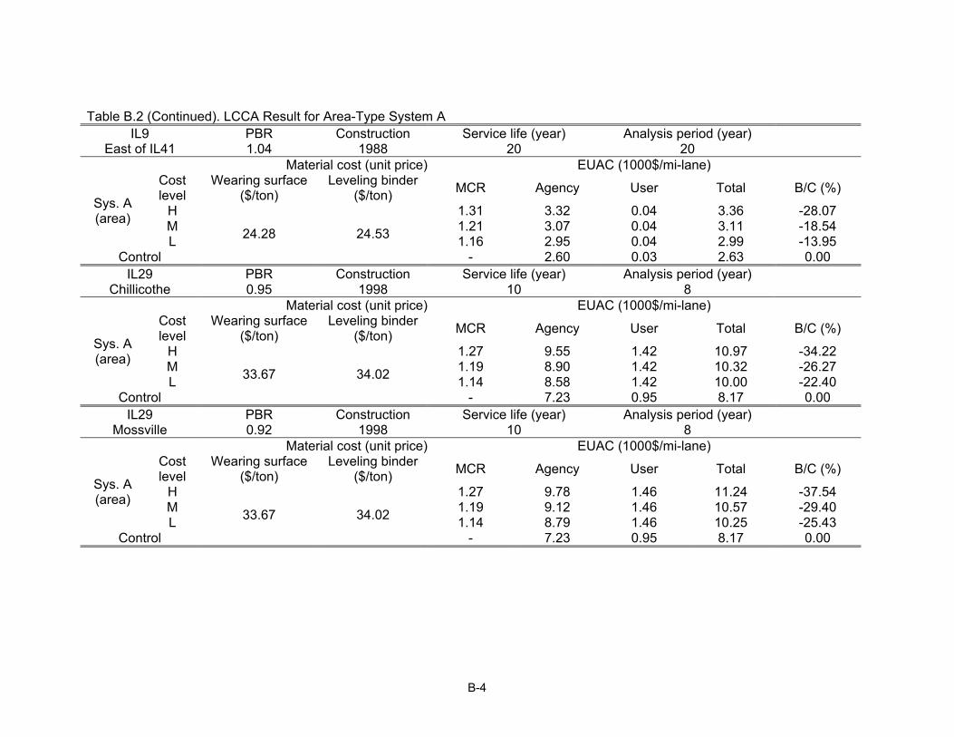
B-4

Table B.2 (Continued). LCCA Result for Area-Type System A IL9

East of IL41 PBR Construction Service life (year) Analysis period (year) 1.04 1988 20 20

Material cost (unit price) EUAC (1000$/mi-lane)

Sys. A (area)

Cost level

Wearing surface ($/ton)

Leveling binder ($/ton) MCR Agency User Total B/C (%)

H

24.28 24.53

1.31 3.32 0.04 3.36 -28.07 M 1.21 3.07 0.04 3.11 -18.54 L 1.16 2.95 0.04 2.99 -13.95

Control - 2.60 0.03 2.63 0.00 IL29

Chillicothe PBR Construction Service life (year) Analysis period (year) 0.95 1998 10 8

Material cost (unit price) EUAC (1000$/mi-lane)

Sys. A (area)

Cost level

Wearing surface ($/ton)

Leveling binder ($/ton) MCR Agency User Total B/C (%)

H

33.67 34.02

1.27 9.55 1.42 10.97 -34.22 M 1.19 8.90 1.42 10.32 -26.27 L 1.14 8.58 1.42 10.00 -22.40

Control - 7.23 0.95 8.17 0.00 IL29

Mossville PBR Construction Service life (year) Analysis period (year) 0.92 1998 10 8

Material cost (unit price) EUAC (1000$/mi-lane)

Sys. A (area)

Cost level

Wearing surface ($/ton)

Leveling binder ($/ton) MCR Agency User Total B/C (%)

H

33.67 34.02

1.27 9.78 1.46 11.24 -37.54 M 1.19 9.12 1.46 10.57 -29.40 L 1.14 8.79 1.46 10.25 -25.43

Control - 7.23 0.95 8.17 0.00

B-5

Table B.2 (Continued). LCCA Result for Area-Type System A US136

East of San Jose PBR Construction Service life (year) Analysis period (year) 1.39 1999 9 9

Material cost (unit price) EUAC (1000$/mi-lane)

Sys. A (area)

Cost level

Wearing surface ($/ton)

Leveling binder ($/ton) MCR Agency User Total B/C (%)

H

34.32 34.67

1.27 7.88 0.23 8.11 -0.27 M 1.19 7.34 0.23 7.57 6.40 L 1.14 7.08 0.23 7.31 9.56

Control - 7.88 0.21 8.09 0.00 IL148

Christopher PBR Construction Service life (year) Analysis period (year) 1.32 1998 10 10

Material cost (unit price) EUAC (1000$/mi-lane)

Sys. A (area)

Cost level

Wearing surface ($/ton)

Leveling binder ($/ton) MCR Agency Sys. A

(area) Cost level Wearing surface ($/ton)

H

33.67 34.02

1.27 7.36 0.18 H 33.67 M 1.19 6.86 0.18 M 1.42 L 1.14 6.61 0.18 L 4.84

Control - 7.06 0.34 Control 0.00 IL111

Pontoon Beach PBR Construction Service life (year) Analysis period (year)

1 1994 14 14 Material cost (unit price) EUAC (1000$/mi-lane)

Sys. A (area)

Cost level

Wearing surface ($/ton)

Leveling binder ($/ton) MCR Agency User Total B/C (%)

H

30.43 30.75

1.27 6.12 0.88 7.00 -29.14 M 1.19 5.71 0.88 6.59 -21.55 L 1.14 5.51 0.88 6.39 -17.87

Control - 4.81 0.61 5.42 0.00

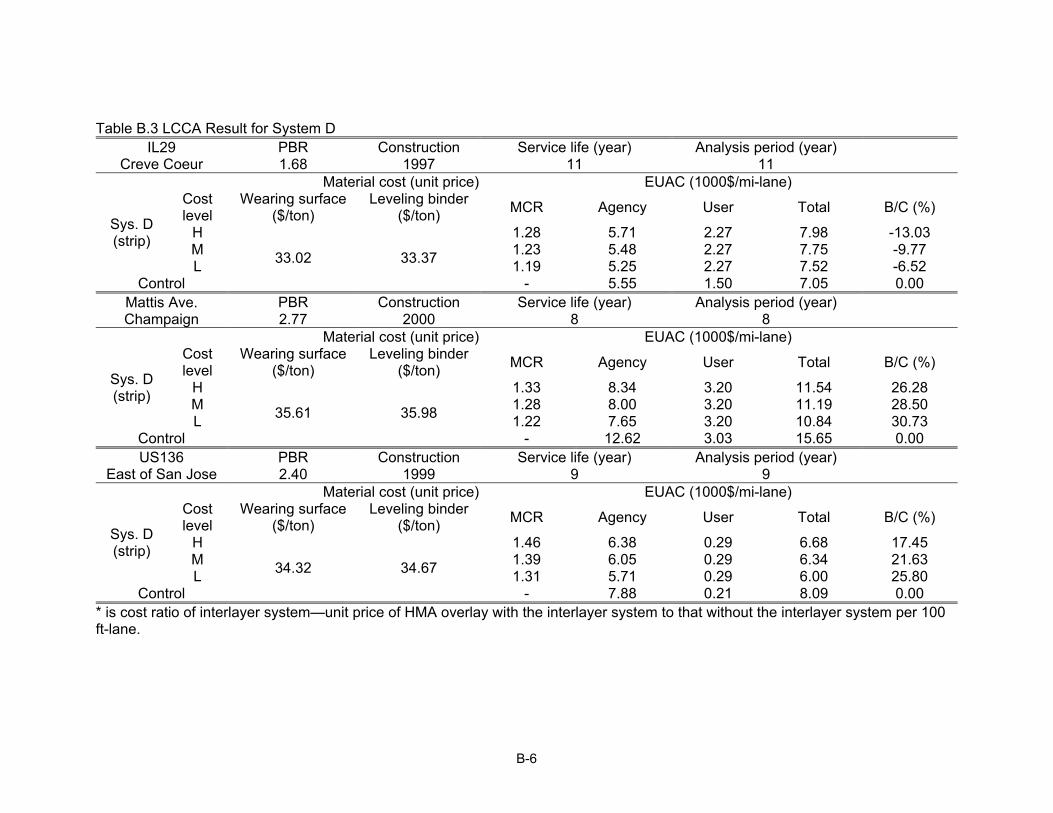
B-6

Table B.3 LCCA Result for System D IL29

Creve Coeur PBR Construction Service life (year) Analysis period (year) 1.68 1997 11 11

Material cost (unit price) EUAC (1000$/mi-lane)

Sys. D (strip)

Cost level

Wearing surface ($/ton)

Leveling binder ($/ton) MCR Agency User Total B/C (%)

H

33.02 33.37

1.28 5.71 2.27 7.98 -13.03 M 1.23 5.48 2.27 7.75 -9.77 L 1.19 5.25 2.27 7.52 -6.52

Control - 5.55 1.50 7.05 0.00 Mattis Ave. Champaign

PBR Construction Service life (year) Analysis period (year) 2.77 2000 8 8

Material cost (unit price) EUAC (1000$/mi-lane)

Sys. D (strip)

Cost level

Wearing surface ($/ton)

Leveling binder ($/ton) MCR Agency User Total B/C (%)

H

35.61 35.98

1.33 8.34 3.20 11.54 26.28 M 1.28 8.00 3.20 11.19 28.50 L 1.22 7.65 3.20 10.84 30.73

Control - 12.62 3.03 15.65 0.00 US136

East of San Jose PBR Construction Service life (year) Analysis period (year) 2.40 1999 9 9

Material cost (unit price) EUAC (1000$/mi-lane)

Sys. D (strip)

Cost level

Wearing surface ($/ton)

Leveling binder ($/ton) MCR Agency User Total B/C (%)

H

34.32 34.67

1.46 6.38 0.29 6.68 17.45 M 1.39 6.05 0.29 6.34 21.63 L 1.31 5.71 0.29 6.00 25.80

Control - 7.88 0.21 8.09 0.00 * is cost ratio of interlayer system—unit price of HMA overlay with the interlayer system to that without the interlayer system per 100 ft-lane.

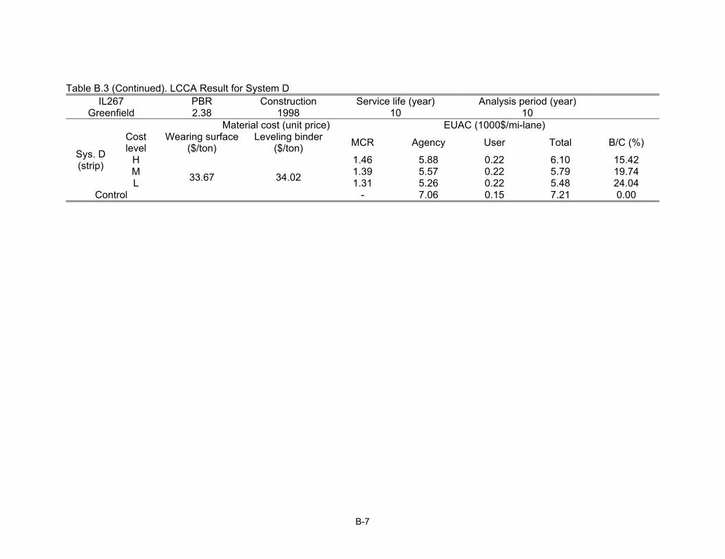
B-7

Table B.3 (Continued). LCCA Result for System D IL267

Greenfield PBR Construction Service life (year) Analysis period (year) 2.38 1998 10 10

Material cost (unit price) EUAC (1000$/mi-lane)

Sys. D (strip)

Cost level

Wearing surface ($/ton)

Leveling binder ($/ton) MCR Agency User Total B/C (%)

H

33.67 34.02

1.46 5.88 0.22 6.10 15.42 M 1.39 5.57 0.22 5.79 19.74 L 1.31 5.26 0.22 5.48 24.04

Control - 7.06 0.15 7.21 0.00

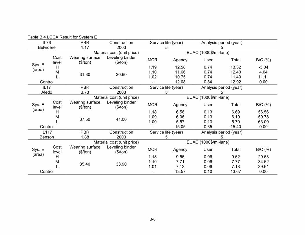
B-8

Table B.4 LCCA Result for System E IL76

Belvidere PBR Construction Service life (year) Analysis period (year) 1.17 2003 5 5

Material cost (unit price) EUAC (1000$/mi-lane)

Sys. E (area)

Cost level

Wearing surface ($/ton)

Leveling binder ($/ton) MCR Agency User Total B/C (%)

H

31.30 30.60

1.19 12.58 0.74 13.32 -3.04 M 1.10 11.66 0.74 12.40 4.04 L 1.02 10.75 0.74 11.49 11.11

Control - 12.08 0.84 12.92 0.00 IL17

Aledo PBR Construction Service life (year) Analysis period (year) 3.73 2003 5 5

Material cost (unit price) EUAC (1000$/mi-lane)

Sys. E (area)

Cost level

Wearing surface ($/ton)

Leveling binder ($/ton) MCR Agency User Total B/C (%)

H

37.50 41.00

1.18 6.56 0.13 6.69 56.56 M 1.09 6.06 0.13 6.19 59.78 L 1.00 5.57 0.13 5.70 63.00 Control - 15.05 0.35 15.40 0.00 IL117

Benson PBR Construction Service life (year) Analysis period (year) 1.88 2003 5 5

Material cost (unit price) EUAC (1000$/mi-lane)

Sys. E (area)

Cost level

Wearing surface ($/ton)

Leveling binder ($/ton) MCR Agency User Total B/C (%)

H

35.40 33.90

1.18 9.56 0.06 9.62 29.63 M 1.10 7.71 0.06 7.77 34.62 L 1.01 7.12 0.06 7.18 39.61 Control - 13.57 0.10 13.67 0.00

B-9

Table B.4 (Continued). LCCA Result for System E IL130 Philo

PBR Construction Service life (year) Analysis period (year) 1.27 2003 5 5

Material cost (unit price) EUAC (1000$/mi-lane)

Sys. E (area)

Cost level

Wearing surface ($/ton)

Leveling binder ($/ton) MCR Agency User Total B/C (%)

H

48.50 49.00

1.17 15.65 0.63 16.28 5.41 M 1.08 14.53 0.63 15.16 11.93 L 1.00 13.41 0.00 13.41 22.09 Control - 16.44 0.77 17.21 0.00 US136

East of San Jose PBR Construction Service life (year) Analysis period (year) 1.85 1999 9 9

Material cost (unit price) EUAC (1000$/mi-lane)

Sys. E (area)

Cost level

Wearing surface ($/ton)

Leveling binder ($/ton) MCR Agency User Total B/C (%)

H

34.32 34.67

1.18 5.97 0.13 6.10 24.56 M 1.09 5.58 0.13 5.71 29.35 L 1.01 5.11 0.13 5.24 35.18 Control - 7.88 0.21 8.09 0.00 US136

West of San Jose PBR Construction Service life (year) Analysis period (year) 1.28 1998 10 10

Material cost (unit price) EUAC (1000$/mi-lane)

Sys. E (area)

Cost level

Wearing surface ($/ton)

Leveling binder ($/ton) MCR Agency User Total B/C (%)

H

33.67 34.02

1.18 6.1 0.1 6.2 1.7 M 1.09 5.6 0.1 5.7 8.7 L 1.01 5.2 0.1 5.3 15.7 Control - 6.1 0.2 6.3 0.00

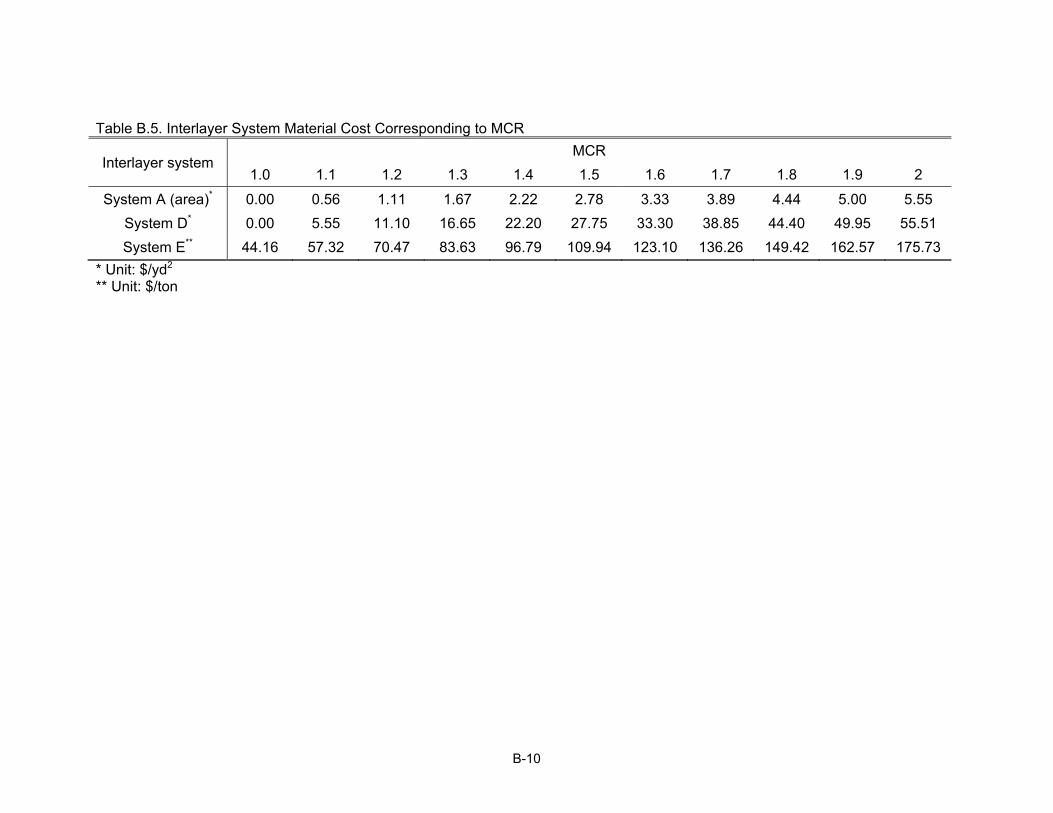
B-10

Table B.5. Interlayer System Material Cost Corresponding to MCR

Interlayer system MCR

1.0 1.1 1.2 1.3 1.4 1.5 1.6 1.7 1.8 1.9 2

System A (area)* 0.00 0.56 1.11 1.67 2.22 2.78 3.33 3.89 4.44 5.00 5.55 System D* 0.00 5.55 11.10 16.65 22.20 27.75 33.30 38.85 44.40 49.95 55.51 System E** 44.16 57.32 70.47 83.63 96.79 109.94 123.10 136.26 149.42 162.57 175.73

* Unit: $/yd2 ** Unit: $/ton