CITY SIZES, HOUSING COSTS, AND WEALTH

Luci Ellis and Dan Andrews

Research Discussion Paper2001-08

October 2001

Economic Research DepartmentReserve Bank of Australia

This paper began from numerous discussions with Paul Bloxham. The authorsthank colleagues and participants in seminars at the Reserve Bank for usefulcomments. Responsibility for any remaining errors rests with the authors. Theviews expressed in this paper are those of the authors and should not be attributedto the Reserve Bank.

Abstract

Australia’s household sector appears to hold a greater proportion of its wealthin dwellings than do households in other countries. Average dwelling prices inAustralia also appear to be high relative to household income, but dwellings inAustralia are not noticeably higher in quality than those in comparable countries.This concentration of wealth in housing also does not seem attributable togovernment policies that encourage dwelling investment in Australia to a greaterextent than is true overseas. A possible reconciliation of this pattern may bethe unusual concentration of Australia’s population in two large cities. Averagehousing prices tend to be higher in larger cities than smaller ones. Therefore,the expensive cities in Australia drag up the average level of dwelling pricesmore than in other countries, resulting in a higher share of wealth concentratedin housing. The increasing importance of dwelling wealth in Australia over recentyears largely reflects the consequences of disinflation and financial deregulation.This is most likely a transitional effect, and the ratio of dwelling wealth to incomeshould stabilise, or begin to grow more slowly, in the future.

JEL Classification Numbers: G12, R11, R31Keywords: dwelling prices, rank-size rule, Zipf’s Law

ii

Table of Contents

1. Introduction 1

2. Dwellings and Household Wealth 3

2.1 Measuring Dwelling Wealth 3

2.2 The Relative Attractiveness of Dwelling Wealth 7

2.3 Dwelling Prices in Different Cities 10

3. The Distribution of City Sizes 13

3.1 Zipf’s Law 13

3.2 The Primate City and Deviations from Zipf’s Law 17

3.3 Implications of the Urban Structure for Dwelling Wealth 19

4. Deregulation, Disinflation and Housing Wealth Dynamics 22

5. A Two-factor Model of City Populations 27

6. Conclusion 28

Appendix A: A Model of City Formation and Dwelling Prices 31

Appendix B: Data Sources 39

References 43

iii

CITY SIZES, HOUSING COSTS, AND WEALTH

Luci Ellis and Dan Andrews

1. Introduction

Australia’s household sector appears to hold a greater proportion of its wealthin dwellings than do households in other countries. This does not appear to bedue to greater quality of the housing stock in Australia than in other comparablecountries. Since the measure of dwelling wealth used in household wealthcalculations includes all private dwellings, this difference similarly cannot bedue to differences in home ownership rates. Alternatively, this pattern in thecomposition of wealth could be a consequence of public-policy decisions thatmake the purchase of dwellings relatively more attractive in Australia than incomparable countries.

In this paper, we present evidence against this explanation. We focus instead onan alternative explanation which relies on the observation that housing costs arehigh in Australia’s two largest cities, Sydney and Melbourne. Housing is usuallymore expensive in large cities than in smaller cities, particularly those cities thatdominate other urban regions. The two largest cities in Australia account for amuch larger proportion of the total urban population in Australia than is the casein most other developed countries. Therefore, the expensive cities in Australiaraise the average level of dwelling prices more than in other countries, resulting ina higher share of wealth concentrated in housing.

This concentration of population in the two largest cities is a result of the unusualstructure of Australia’s urban population. To a first approximation, the populationsof cities in many countries are in inverse proportion to their ranking by populationsize; that is, the second-largest city is roughly half the size of the largest, thethird-largest one-third the size and so on. This empirical regularity is an exampleof a power law, and is known as the rank-size rule or Zipf’s Law. Australia’slarge towns and cities follow an approximate rank-size power law, but with aflatter distribution than other countries. Sydney and Melbourne together thereforeaccount for ‘too much’ of the urban population of Australia, raising the nationalaverage price of dwellings and the share of dwellings in household wealth.

2

Although this geographic explanation for the structure of Australian households’balance sheets is not the only plausible one, it is consistent with the data and doesnot rely on presumed differences in preferences. The available data do not suggestthat Australians have a greater preference for housing than residents of otherdeveloped economies, or that government policy encourages dwelling investmentto a greater extent than does policy elsewhere.

The characteristics of housing also support a geographical explanation. Housingdiffers from the standard neoclassical good; it is heterogenous and its spatialfixity means that the location of the housing stock matters to households (Smith,Rosen and Fallis 1988). Housing is thus imperfectly substitutable across locations(Maclean 1994). These factors, combined with construction lags make housingsupply inelastic in the short run, so the housing market is prone to rapid increasesin dwelling prices (housing price booms). The relative dominance of the largercities may therefore also help explain Australia’s susceptibility to housing-pricebooms. In countries with less concentrated urban populations, price booms in onecity have less effect on national average prices.

To the extent that average dwelling prices are higher in Australia, some householdsmight respond by reducing their demand for housing services. At the margin,renters would shift their consumption away from housing and downgrade tolower-quality dwellings. However, owner-occupiers’ housing demand is both aconsumption and investment decision, so their response is less clear (Hendersonand Ioannides 1983). It seems likely that any demand substitution would onlypartially offset the initial increase in dwelling prices.

The question of why Australia’s population structure is different remains. Thebroad similarity with Canada suggests that our federal structure has resulted instate capital cities acting as primate cities dominating the surrounding regions.This will tend to flatten out the rank-size relationship. It is also possible that largecountries with small populations – like Canada but unlike the United Kingdom –have flatter rank-size relationships because the large distances between populationcentres increase transport costs. If so, the structure of the household balance sheetin Australia would not require a policy response, but rather would be partly anecessary implication of our geography and political history.

The paper proceeds as follows. In the next section, we document the importanceof dwelling wealth in the household sector’s balance sheet in Australia and other

3

developed countries, and critically examine some possible explanations of thehigh level in Australia. Section 3 provides a brief overview of the literature andempirical evidence about the distribution of city sizes. The data confirm thatZipf’s Law is a reasonable first approximation to the distribution of city sizes.We also show that Australia’s urban structure accounts for around one-third of thedifference between the wealth-income ratios in Australia and the United States.

Section 4 shows that the effects of urban structure on national average housingprices might only occur if households’ financial behaviour is not constrained byeither financial regulation or the interaction between capital market imperfectionsand inflation. Section 5 develops a simple model of city sizes with housing costsconsistent with the observation that larger cities have more expensive housing.Therefore, the more important are the large cities in the total population, the higherwill be the national average level of dwelling costs. The conclusion in Section 6draws out some of the macroeconomic implications of Australia’s relatively largeshare of dwellings in household wealth, and in particular, argues that a dramaticfall in dwelling prices is unlikely.

2. Dwellings and Household Wealth

2.1 Measuring Dwelling Wealth

Measurement of the value of the stock of dwelling wealth is in principle assimple as counting the number of dwellings, and multiplying by an appropriatelyweighted estimate of the average prices of those dwellings. The first part can begenerated in a straightforward way using national census data, and interpolatedbetween census dates using information on dwelling completions. The secondpart, which must be available in local currency values rather than as an indexnumber (as is the case with the ABS House Price Index), is more difficult to obtain.

Some statistical agencies publish estimates of the value of the dwelling stock aspart of the country’s national accounts. However, national accounting principlesdo not capture the market price of dwellings, including land value, which iswhat matters for household wealth. Similarly, implicit price deflators for dwellinginvestment from national accounts do not correspond to market prices of theexisting dwelling stock because they generally exclude land and are based on thecomposition of new dwellings, not the stock of existing dwellings. Price deflators

4

also exclude the effects of increasing dwelling quality, for example where newhouses are larger on average than those built previously. However, these effectsclearly add to households’ dwelling wealth.

The most appropriate sources for data on the market value of dwellings are thosebased on prices of existing dwellings sold. These series are sometimes collectedby national statistical agencies but are more likely to be published by financialinstitutions or real estate associations. Dwelling prices are frequently used as anindicator of more general price pressures (Girouard and Blondal 2001). Thereforemany published series on sale prices abstract from compositional effects, or relateonly to specific markets or types of housing – for example, detached houses inmajor urban areas, houses for which past sale prices are known, or dwellings ofa standardised size. These adjustments ensure that the series are close to a pureprice signal, but are unhelpful when trying to determine the market value of thetotal dwelling stock.

Appropriate measures of the market price of dwellings must include all regionsof the country, and apartments and townhouses as well as detached houses. Forthis reason, the Reserve Bank uses data from the Housing Industry Association’sHousing Report, based on prices paid by customers of the CommonwealthBank. Unlike the other dwelling price series available in Australia such asthose from the Real Estate Institute of Australia (REIA) and the ABS, thesedata include all dwellings, not just detached houses, and cover non-metropolitanregions. However, we are therefore implicitly assuming that Commonwealth Bankcustomers are representative of all home-buyers. The CBA/HIA prices tend to behigher than those reported by the REIA; it is difficult to say which is correct,given that the CBA/HIA series is otherwise conceptually superior. However, ifthe CBA/HIA data did overstate the true level of housing prices in Australia, wewould have a smaller distance from the dwelling wealth levels of other countriesto explain.

Even when conceptually correct measures of sale prices are available, someaspects of their construction can still create biases in estimates of dwelling stockvalues. Measured values can be biased down by the use of median rather thanaverage prices, for what is likely to be a left-skewed distribution. There is also apotential bias in average dwelling-price measures if different types of dwellingsturn over at different rates: the composition of dwellings sold would therefore

5

differ from that of dwellings standing. Countries with large public-housing sectorscould have overstated dwelling wealth unless these dwellings are excluded.1

Similarly, if privately rented dwellings are owned by corporations, not otherhouseholds, their exclusion could reduce measures of dwelling wealth, especiallyin countries with low owner-occupation rates.2

Table 1: Non-financial Assets as a Share of Total AssetsPer cent

1987 1990 1993 1996 1999

Australia 55 68 63 63 64

Canada 47 46 45 43 42

France 61 57 51 50 na

Germany na 67 65 64 60

Italy 53 51 50 48 na

Japan 65 63 57 51 na

UK 55 55 45 42 42

US 39 38 35 32 28

Sweden(a) 49 53 51 47 45

New Zealand 58 61 57 61 60

Note: (a) 1999 data refer to 1998.Sources: Mylonas, Schich and Wehinger (2000); RBA; RBNZ

With these data caveats in mind, Table 1 shows the shares of non-financial assetsin total household wealth for countries for which we have sufficient data. Althoughthese data include consumer durables for all countries except New Zealand,non-financial assets are dominated by the dwelling stock. A decade and a halfago, Australia’s household balance sheet contained a non-financial asset sharearound the international average. Since then, the share in most other countries hasfallen or stayed fairly constant, while in Australia the share has risen by almost10 percentage points. This divergence is not due to differences in the relativeimportance of financial assets: household holdings of financial assets in Australia

1 The measure of dwelling wealth in household wealth calculations is based upon privatedwellings. Since this measure is expressed as a percentage of household disposable income,the inclusion of public housing would inflate this estimate because households do not ownthem.

2 Whilst this effect is likely to be small in most countries, it will be more important in ContinentalEurope (especially France, Germany and Italy) where some rental housing is financed by largebusinesses.

6

are not particularly low relative to those in other developed countries. Rather,housing is expensive relative to income in Australia.

The ratio of aggregate dwelling wealth to disposable income is roughly equivalentto the ratio of average dwelling prices to average disposable income; the ratioswill only differ to the extent that there is a difference between the number ofprivate-sector dwellings and the number of households (this difference is marginalin Australia).3 Table 2 shows this measure of dwelling prices is relatively highin Australia, and grew fairly steadily through the 1990s, reaching 378 per centby late 2000. While some nations (Japan, UK, Sweden) experienced rapidrun-ups in dwelling prices, these booms ultimately led to busts, and price-incomeratios in those countries returned to levels closer to those in other countries(Henley 1998). Of this group of countries, only New Zealand has followedAustralia in experiencing sustained growth in relative housing prices.

Table 2: Housing Wealth as Per Cent to Household Disposable Income1980 1985 1990 1995 1998

Australia 248 239 281 303 355

Canada 123 – 118 129 129

France(a) 172 – 218 218 227

Germany(a) – – 331 302 301

Italy 133 – 170 172 166

Japan(b) 380 397 641 429 381

UK 343 357 361 252 293

US 169 170 173 155 163

Sweden(b) 208 184 245 182 198

New Zealand 185 237 243 278 283

Notes: (a) 1998 data refer to 1997.(b) Figures refer to non-financial assets which include consumer durables as well as dwellings.

Sources: Bundesbank; Mylonas et al (2000); OECD; RBA; RBNZ

Some increase in dwelling prices should have been expected through the 1990s inAustralia. Following financial deregulation, households now enjoy greater accessto loan finance for the purchase of dwellings. Reinforcing this trend, the moveto low inflation over that period enabled households to service larger mortgagesand therefore purchase more expensive homes (Stevens 1997). These factors

3 Holiday homes and vacant rental properties can result in the number of private-sector dwellingsexceeding the number of households.

7

would be expected to increase demand for dwellings and put upward pressure ondwelling prices. Household indebtedness also increased substantially during thisperiod, reflecting these changes, bringing Australia to around the average level ofindebtedness seen in other comparable countries; we discuss these issues in moredetail in Section 4. However, these changes do not explain why the increase indwelling prices since the 1990s has resulted in Australia having relatively moreexpensive housing than other low-inflation countries. These changes explain theincrease in dwelling prices and indebtedness, but not why the price level hasincreased from around the average to well above international averages.

This divergence in the dwelling wealth-income ratio, if sustained, implies thatdifferent countries have different relative prices of housing in the long run.We consider an explanation for this based on unobservable and unexplaineddifferences in preferences for housing to be unsatisfactory, and inconsistent withthe evidence on housing quality presented in Table 4. The ranking of countriesby dwelling wealth-income ratio does not obviously follow differences in averageincome, so these variations in the relative price of housing are also not obviouslyattributable to housing services being either a superior or inferior good.

2.2 The Relative Attractiveness of Dwelling Wealth

Despite the limitations of the data presented in the previous section, they clearlysuggest that Australians have concentrated a larger portion of their wealth inhousing than their counterparts in other developed economies, and spend a largerproportion of their incomes to purchase a home. The first step in finding thereasons for this result is to establish whether there are government policies orother factors that could have contributed to it. Tax policies such as exclusion fromcapital gains tax can make owner-occupied dwellings relatively more attractivethan other forms of investment, and thus cause over-investment in dwellings.It is also important to assess whether there is a greater revealed preference fordwellings in the sense of their being larger or higher-quality in Australia thanelsewhere. Tables 3 and 4 present indicators for these factors for Australia and theother countries for which we have dwelling wealth data.

8

Table 3: Policies Affecting the Relative Attractiveness of Housing WealthMortgage interest

deductibilityCapital gains

exemption on familyhome

Share ofpublic

housingPer cent

Memo item:home ownership

rates

Australia No Yes 5�1 70�1

Canada No Yes 1�7 63�7

France Yes(a) Yes 17�0 56�0

Germany Yes Yes 26�0 43�0(b)

Italy Yes(c) Yes 6�0 68�0

Japan No No(d) 7�0 60�3

UK Yes(e) Yes 24�0 69�0

US Yes Yes(f) 1�2 67�4

Sweden Yes No 22�0(g) 56�0

New Zealand No Yes 6�4 71�2

Notes: Data are latest available. See Appendix B for detailed information on sources and reference periods. Thereare other more targeted policies that encourage homeownership across countries (Miron 2001). Althoughthese policies can vary across countries, their net effect seems less significant because their coverage isgenerally limited.(a) Interest is deductible for the first five years. The deduction is equivalent to 25 per cent of the totalinterest bill, subject to a ceiling based on the date of the contract and age of the building.(b) West Germany only.(c) A tax credit of 27 per cent of interest payments is allowed up to a ceiling.(d) A special deduction of U30 000 000 can be claimed for the principal residence.(e) Mortgage interest deductible only on the first £30 000 of a mortgage.(f) Capital gains is theoretically subject to tax. However, any capital gains from the sale of the family homewhen another dwelling costing at least as much is purchased within two years of the sale is exempt fromtaxation. A once-in-a-lifetime exclusion of US $125 000 also exists for people over 55 years.(g) Excludes co-operative sector.

Owner-occupied housing is tax-advantaged in Australia, but some developedcountries apply an even greater range of tax incentives toward home ownership,including deductibility of mortgage interest payments (Table 3). Past theoreticalwork suggests that deductibility of mortgage interest represents a greater distortionthan capital gains tax exemption (Britten-Jones and McKibbin 1989).4 On this

4 One policy encouraging home ownership in Australia that is not seen elsewhere is the exclusionof owner-occupied dwellings from means and assets tests that can restrict access to governmentpensions. This encourages pensioners to hold onto larger homes rather than trade downto something smaller, thus restricting the supply of family-sized homes available to largerhouseholds. This tax advantage to owner-occupied housing is not applicable in other countriesbecause their welfare systems are not means tested in the same way.

9

basis, we would expect that if anything, Australia’s housing stock is less affectedby over-investment than those of some other developed countries.

The quality of the Australian dwelling stock is comparable with that in someother countries. However, Australia has a greater proportion of detached houses,suggesting somewhat more land-intensive housing patterns, and the share ofrelatively new homes built in the past 20 years is somewhat higher, due toAustralia’s relatively high population growth (Table 4). Dwellings in Australiaappear to be similar in size to those in other non-European developed countries.Although dwellings are larger on average here than in Europe, this is partlybecause households are larger; the number of persons per room is around theaverage for developed countries.

Table 4: Indicators of Housing QualityPersons

per roomAverageexistingdwelling

size

Averagenew

dwellingsize

Houses Detachedhouses

Dwellingswith sixor morerooms

Dwellingsbuilt since

1980

m2 Per cent of stock

Australia 0�6 131�8(c) 185�5 87�6 78�8 63�5 33�7

Canada 0�5 114�0 na 66�4 55�9 75�0(d) na

France 0�7 88�0 102�5 56�2 na 16�6 32�0(e)

Germany(a) 0�5 86�7 101�9 45�6 31�0 11�5 22�0

Italy 0�8 92�3 88�7 na na na na

Japan 0�7 89�6 94�3 na 59�2 na 51�8

UK 0�6 84�0(f) 76�0 80�7(f) 25�6 36�8 13�3

US 0�5 156�5 199�7 66�7 60�6 45�2 25�4

Sweden 0�5 89�8 86�0 45�7 na na 12�0

New Zealand(b) 0�5 132�0 na 83�0 73�0 56�1 na

Notes: Data are latest available. Proportion of houses in dwellings refers to all single-family dwellings includingtownhouses and terraces. See Appendix B for detailed information on sources and reference periods.(a) West Germany only. Dwellings built column refers to dwellings built since 1979, not 1980.(b) Existing dwelling size and detached house data refer to Auckland.(c) Excludes public housing.(d) Refers to five or more rooms. The average number of rooms in Canada is six.(e) Since 1975.(f) England only.

The rate of home ownership in Australia is higher than a number of thecountries shown in Table 3, but there are many other countries with similarownership rates, including New Zealand, Finland, Ireland, Greece and Spain

10

(European Parliament 1996). Home ownership tends to increase average housingprices because owner-occupiers internalise the cost of the wear and tear theycreate in their home, while renters might not fully bear such costs (Hendersonand Ioannides 1983). Owner-occupiers therefore require a lower gross return thanlandlords, and are thus in theory willing to pay more for a given dwelling in theabsence of differences in tax treatment.

On the other hand, ownership of private rental properties also attracts favourabletax treatment in many OECD countries (Miron 2001). Negative gearing taxprovisions in many countries allow landlords to deduct interest payments againstincome from other sources if they exceed rental income net of expenses, while taxcredits and loan subsidies apply in France (Cardew, Parnell and Randolph 2000).These tax provisions generally ensure that owners of rented dwellings receive thesame tax treatment as owners of other commercial properties (Weicher 2000).Since they are common across developed countries, Australia’s negative gearingprovisions do not represent a relatively greater incentive to invest in rentalproperties. In the UK by contrast, mortgage interest cannot be deducted againstrental or other income (Miron 2001). This may be discouraging the expansion ofthe existing small private rental sector there.

Although previous studies have found evidence of over-investment in housing inAustralia, the evidence that this over-investment is greater than in other countriesis weak (Bourassa and Hendershott 1992). Therefore tax policies do not appear toexplain the divergence in the stock of housing wealth between Australia and otherdeveloped countries; to do so, the incentives for over-investment would have tobe stronger here than elsewhere. The concern about over-investment is probablybetter directed at countries that allow tax deductibility of interest payments onowner-occupiers’ mortgages (Mills 1987).

2.3 Dwelling Prices in Different Cities

Figure 1 indicates that city sizes and city-level house prices are related. Althoughcity-specific factors also matter, larger cities usually have higher average housingprices than smaller cities in the same country, even after allowing for variation in

11

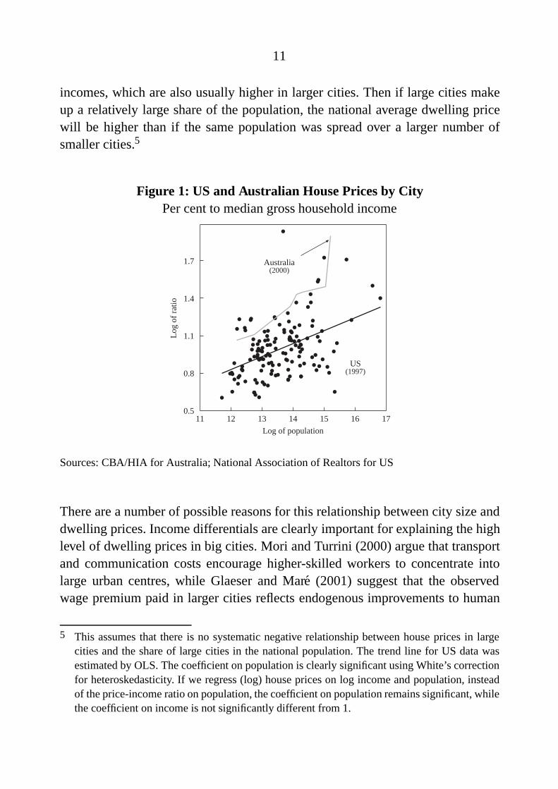
incomes, which are also usually higher in larger cities. Then if large cities makeup a relatively large share of the population, the national average dwelling pricewill be higher than if the same population was spread over a larger number ofsmaller cities.5

Figure 1: US and Australian House Prices by CityPer cent to median gross household income

��

�

��

�

��

���

�

�

�

�

�

���

��

��

��

�

�

��

���

�

�

��

�

�

��

�

�

�

�

�

�

���

���

�

����

� �

�

�

�

�

�� �

�

���

�

�

�

�

�� ��

�

��

�� �

�

�

���

�

��

�

��

��

�

���

��

�

��

�

�

�

��

�

�

��

���

�

�

��

�

��

��

�

�

�

�

�

���

�

�

� ��

0.5

0.8

1.1

1.4

1.7

11 12 13 14 15 16 17

Log

of

ratio

Australia

US

Log of population

(1997)

(2000)

Sources: CBA/HIA for Australia; National Association of Realtors for US

There are a number of possible reasons for this relationship between city size anddwelling prices. Income differentials are clearly important for explaining the highlevel of dwelling prices in big cities. Mori and Turrini (2000) argue that transportand communication costs encourage higher-skilled workers to concentrate intolarge urban centres, while Glaeser and Mare (2001) suggest that the observedwage premium paid in larger cities reflects endogenous improvements to human

5 This assumes that there is no systematic negative relationship between house prices in largecities and the share of large cities in the national population. The trend line for US data wasestimated by OLS. The coefficient on population is clearly significant using White’s correctionfor heteroskedasticity. If we regress (log) house prices on log income and population, insteadof the price-income ratio on population, the coefficient on population remains significant, whilethe coefficient on income is not significantly different from 1.

12

capital arising from lower search costs and greater specialisation. However, thiscannot be the whole story, as dwelling prices are high relative to income inlarger cities, as well as in absolute terms (Figure 1; Table 5).6 This may bebecause housing demand represents an increasing share of expenditure as incomeincreases: preferences may not be homothetic or wealth may increase faster thanincome.7 Other reasons include that larger cities offer more amenities and a greaterrange of job opportunities. In equilibrium, these benefits will be balanced againstgreater costs, such as congestion, crime and higher housing costs (Gabaix 1999b).

Table 5: Dwelling Prices by City Relative to Disposable Income, 1998/99City Population Average income Dwelling price-income ratio

’000 Per cent of nationalaverage

Disposable income Gross income

Sydney 4 041.4 113�1 8.06 5�64

Melbourne 3 417.2 113�2 4.69 3�51

Brisbane 1 601.4 97�1 5.16 3�92

Perth 1 364.2 100�4 4.87 3�76

Adelaide 1 092.9 91�4 4.21 3�47

Canberra 348.6 124�7 3.83 2�94

Hobart 194.2 93�3 3.38 2�58

Notes: These price-income ratios are not strictly comparable with the national data in Table 2. Survey dataunderstate national accounts disposable income, and number of households does not equal the numberof dwellings.

Sources: See Appendix B

6 As shown in Figure 1, the divergence increased between 1998 and 2000. Canadian housingprices also show a roughly rising relationship, but this is dominated by unusually high housingprices in British Columbia and low prices in Quebec.

7 It might also be because large cities are space-constrained, limiting supply and putting upwardpressure on dwelling prices.

13

3. The Distribution of City Sizes

3.1 Zipf’s Law

Australia’s apparently more expensive housing does not seem to be due todifferences in government policy or household preferences. An alternativecandidate explanation for the importance of housing wealth in Australia is that theurban population is concentrated in two large cities with relatively high housingcosts. In most developed and many developing countries, the population size andpopulation ranks of cities are distributed approximately according to a powerlaw. This means that if a country’s urban centres are ordered by population size,the rank of city S (largest � 1, second-largest � 2, and so on) has an inverserelationship with its population p�S�:

S �a

p�S�ζ(1)

where a and ζ are positive constants. This empirical regularity can bedemonstrated graphically by plotting the natural logarithm of the rank of eachcity against the natural logarithm of its population size. Figures 2–4 showthis relationship for a range of developed and developing countries. When theexponent ζ equals 1, this empirical regularity is known as Zipf’s Law (Zipf 1949),corresponding to a slope of �1 for the lines in these figures.8

8 Gabaix (1999b) showed that cities with populations that grew randomly would converge to adistribution matching Zipf’s Law (ζ � 1) in its upper tail, provided that the growth rates forall cities were drawn from a statistical distribution with the same mean and variance, and thatthe cities were bounded to be above some minimum size. The existence of such a commondistribution is called Gibrat’s Law. If this is not true, then Zipf’s Law does not hold; Zipf’s Lawshould therefore be seen as a diagnostic for the underlying growth process, rather than a lawthat must hold in all cases and at all times. Earlier work on explaining Zipf’s Law centred onvariations of this requirement for random growth from a common distribution. Simon (1955)developed a simple model with additions to the population attaching to existing cities withprobability equal to its share of total population. Hill (1974) formalised this proportionality ofprobability to population as a Bose-Einstein occupancy problem. Gibrat’s Law has also beenused to study the size distributions of firms, income distributions and other economic variables;see Sutton (1997) for a review.

14

Figure 2: Rank-size Relationship – G7 Countries

0

1

2

3

4

5

11 12 13 14 15 16 17

Log

of

rank

US

Japan

France

Germany

Canada

UK

Italy

Log of population

Figure 3: Rank-size Relationship – Other Developed Countries

0

1

2

3

4

5

10 11 12 13 14 15 16 17

US

Netherlands

Spain

Australia

Switzerland

Belgium

Log of population

Log

of

rank

Some empirical support for Zipf’s Law has been shown for US cities throughtime (Krugman 1996; Ioannides and Dobkins 2000), while international evidencehas been more mixed (Kamecke 1990). Recent literature on this power law haspresented OLS estimates of the slope of this ‘Zipf curve’ as evidence of theexponent ζ being 1. Although OLS is not an ideal estimation method when the

15

Figure 4: Rank-size Relationship – Developing Countries

0

1

2

3

4

5

6

10 11 12 13 14 15 16 17

China

India

Brazil

Russia Indonesia

Ukraine

Argentina

Poland

Log of population

Log

of

rank

left-hand side variable is the log of an integer, maximum-likelihood estimates givesimilar results (Kamecke 1990; Urzua 2000).9

Although the evidence is mixed, a power law seems to be a reasonable firstapproximation of the data for many countries. In contrast, models of city formationbased on economic first principles such as the location decisions of workers andowners of capital have generally failed to capture the size distribution seen in thedata. For example, Henderson’s (1974) model could only generate city sizes thatvaried at all by introducing different traded-goods industries facing (unexplained)differences in production-function parameters; there was no mechanism forgenerating the observed power law except by assumption. It would be equallymisguided, however, to develop a theory that could only generate a Zipf-typepower law distribution.

As indicated in the figures above, the rank-size relationship of Australian citiesdiffers noticeably from the predictions of Zipf’s Law, and the relationships seenin other countries. This is confirmed by estimates of the power law exponent �ζ�

9 The OLS estimates are based on an inappropriate specification of the errors, so their standarderrors and t-statistics are not meaningful and we have not reported them here. The residuals forboth sets of estimates have a cyclical pattern; similar-sized cities tend to have residuals of thesame sign. Explaining this is beyond the scope of the paper, but it suggests that there is more tothe city-size distribution than a simple power law.

16

Table 6: Indicators of City Population StructureZipf curve exponent estimates Share of urban

population inPrimacy ratio(a)

OLS MLE two largest cities

Argentina 0�68 0�80 68.7 8�92

Australia 0�62 0�71 54.2 1�18

Belgium 0�92 1�28 47.7 1�44

Brazil 1�22 1�19 26.8 1�77

Canada 0�82 0�82 42.6 1�35

China 1�08 0�56��� 4.6 1�11

France 0�98 0�92 48.8 7�38

Germany 1�28 1�31 20.0 2�04

Indonesia 0�89 0�82 35.1 3�39

Italy 1�14 1�31 27.1 1�96

Japan 1�32 1�21 15.2 2�43

Netherlands 1�24 1�28 28.0 1�02

New Zealand 0�74 � 59.1 2�97

Poland 1�31 1�39 21.4 1�97

Russia 1�18 1�06 19.0 1�97

Spain 1�32 1�36 28.0 1�86

Ukraine 1�11 0�96 20.9 1�64

United Kingdom 1�83 2�23��� 19.0 6�90

United States 1�01 0�76�� 15.7 2�04

Notes: MLE estimates exclude New Zealand due to insufficient number of cities. **,*** indicates related Lagrangemultiplier test of ζ� 1 rejected at 5 per cent and 1 per cent significance levels.(a) Ratio of largest city to second-largest. If Zipf’s Law is true, this ratio should be 2.

Sources: See Appendix B

for different countries (Table 6). The point estimates for Australia using eitherestimation method are below that for all the other countries except China, whichhas a city-size structure completely different from a power law. The plot of logrank against log size for China is nowhere near linear, for reasons we can onlyspeculate about.

Australia’s low ζ implies that city populations are lower further down the rankordering than Zipf’s Law predicts. Indeed, Australia has no middle-sized citiesaccording to the UN definition of between 500 000 and 1 million inhabitants. In1999, Newcastle, the sixth-largest had around 480 000 residents and Adelaide,the fifth-largest city had 1.09 million. By contrast, Australia’s small towns follow

17

Zipf’s Law very closely: estimates of ζ for the set of towns with populationsbetween 5 000 and about 80 000 are very close to 1. This suggests that populationgrowth behaves in roughly the same way across Australia’s small towns, but thatsmall towns as a group behave differently from large towns and cities. The resultis surprising, given that the literature finds that Zipf’s Law usually holds in theupper tail of the city-size distribution (Gabaix 1999b).

Why does Australia have so few middle-sized cities, resulting in such a low ζ inthe upper tail of the city-size distribution? One circumstance where the estimatedZipf coefficient could be lower than 1 is where smaller cities had lower averagegrowth rates or higher variances of their growth rates than the larger cities. Alower mean growth rate could occur if natural population increase is roughlythe same nationwide, but larger cities systematically attract residents away fromsmaller cities. Similarly, smaller cities might have narrower industrial bases andthus be more susceptible to industrial shocks, leading to population growth havinga higher variance than in larger cities (Gabaix 1999b).

3.2 The Primate City and Deviations from Zipf’s Law

Models of the development of city sizes based on random growth from a commondistribution can explain the rank-size rule observed in the population structuresof many countries. However, other countries have only one significant city, or acity that is much larger than would be expected based on the Zipf power law. Inthe geography literature, these are referred to as primate cities (Jefferson 1939).10

Zipf’s Law predicts that the largest city in a country should be double the sizeof the next largest – a good approximation for many countries. In countries withprimate cities, however, it can be six to eight times as large as the next-largestcity, and well out of line with the power law describing the relative sizes of thesmaller cities in that country. The primacy ratio is the ratio of the largest to thesecond-largest city. If Zipf’s Law holds, this primacy ratio should be around 2; ifit is above 3, the largest city is considered a primate city.11

10 Countries with obvious primate cities include Argentina, Denmark, Finland, France, GreeceIndonesia, Norway and the United Kingdom.

11 Thresholds for defining primate cities have evolved over time. Jefferson’s (1939) originaldefinition of a primate city was one that was more than twice as large as the next-largest city,that is, any upward deviation from Zipf’s Law.

18

Australia is often considered to be a country with no primate city. It is certainlytrue that Sydney’s population is substantially less than twice that of Melbourne.Even if Newcastle, Wollongong and the Central Coast are included in Sydney’spopulation as a single conurbation, Sydney’s population is well below what wouldbe predicted from the rank-size relationship of the other cities.

One plausible view of Australia’s urban structure is that each state capital isa primate city for its state, and that its population size relative to other statecapitals is less relevant. Hill (1974) demonstrated that if the cities in each regionof a country follow Zipf’s Law, then the rank-size relationship for the wholecountry will also be approximately consistent with Zipf’s Law. As mentionedearlier, the rank-size distribution for Australian towns with fewer than 80 000inhabitants – that is, smaller than Hobart, the smallest of the state capitals – isclose to that predicted by Zipf’s Law, but larger cities have a flatter rank-sizerelationship. This is consistent with Australia’s nationwide rank-size relationshipbeing a combination of several state rank-size relations where the largest city isa primate, while all the others follow Zipf’s Law. It also clearly suggests thatsmaller towns are subject to random growth of a common nature, while the stateand national capitals evolve according to different forces.

Canada also has a relatively flat rank-size curve and a federal political system.Provincial capitals tend to attract residents from other parts of the provincebecause their positions as the seat of government results in these cities offeringemployment opportunities in administration and policy that are not availableelsewhere.12 Unlike Australia, the provincial capitals in Canada are not usuallythe largest cities in the provinces. This may help explain both why Canada’s Zipfcurve is not as flat as Australia’s, and why dwelling prices are lower there; demandpressures on housing from internal migration will be spread over two cities in eachprovince – the economic centre and the political centre. The difference may reflectthe history of colonisation by European settlers, and this may help explain thecurrent urban structure.

12 These opportunities are in addition to the normal range of private-sector occupations seen in acity of that size, rather than a substitute for them. By contrast, manufactured political capitalssuch as Brasilia, Canberra or Islamabad have narrower employment bases focused on the publicsector. This may explain why these capitals do not become primate cities.

19

Because both these countries have relatively small populations spread over a largearea, transport costs and political institutions may have induced multiple centresof economic activity, resulting in the formation of a primate city for each region.In more densely populated countries such as the United Kingdom, transport costsare less important. A single primate city may arise in those countries, but theremay be little impetus for others to form, as centralised administrative functionscan cover the entire country, without subsidiary regional centres to cover someareas. Ades and Glaeser (1995) found that a relative lack of transport infrastructuretended to foster centralisation into large cities. Sparsely populated countries suchas Australia and Canada have fairly sparse transport infrastructure relative to moredensely populated developed countries. This may be encouraging the relativelyhigh concentration of these countries’ populations into a few cities, albeit on aregional rather than national basis.

3.3 Implications of the Urban Structure for Dwelling Wealth

As a rule, primate cities account for a greater fraction of the total population thanwould a largest city that followed Zipf’s Law. Larger cities tend to have moreexpensive housing than smaller cities, so the national average housing price willbe higher as the primacy ratio rises, even if housing prices in individual citiesare unaffected by this change. Holding national population fixed, an increase inthe primacy ratio (or the concentration of population in the largest city) reducesboth the absolute population and relative share of the other cities, which may beexpected to reduce their average housing prices. Nonetheless, the national averagehousing price will rise if the population share of the largest city rises, givenreasonable assumptions about the functional form of the relationship betweenpopulation and housing prices at the city level.13 This implies that if a primatecity exists, or more generally, the population is concentrated in a few large cities,national average housing costs tend to be higher than would be true if Zipf’s Lawheld.

How important is this urban structure effect? Our best guess is that it accounts forabout one-third of the difference between the dwelling wealth-income ratios of

13 In particular, this will hold if house prices in individual cities are a rising function of populationwith a second derivative that is always non-zero; a proof of this is available on request. Theresult also holds for some cases where h��

� 0 at some point.

20

Australia and the United States. Although this estimate is necessarily rough, webelieve it conveys the correct order of magnitude, if not the exact figure.

Recall Figure 1 in Section 2.3, which showed housing price-income ratios forindividual cities in Australia and the United States. Other than Sydney, the ratiosfor Australian cities are only somewhat above the average value for US cities ofcomparable size, and just above the bounds of US experience. We estimated a lineof best fit for housing price-income ratios in US cities, given their populations(this is the trend line shown on Figure 1). We used the fitted values to derive theprice-income ratios they implied for cities equal in size to each of Australia’smajor cities. Multiplying these ratios by a measure of income for each city,comparable to those used in the disaggregated US data, gives a counterfactualprice for Australian housing (Table 7). These are the prices that would prevail inAustralia if the US relationship between city size and price-income ratios alsoapplied to Australia.

Table 7: Actual and Counterfactual Australian Dwelling Prices by CityPer cent to city-level median household gross income, June quarter 1998

City Actual house prices Counterfactual house prices

Sydney 6�68 3�21

Melbourne 4�24 3�15

Brisbane 4�75 2�92

Perth 4�72 2�87

Adelaide 4�27 2�80

Canberra 3�35 2�49

Hobart 3�31 2�34

Sources: See Appendix B

The counterfactual prices can be aggregated along with actual data fornon-metropolitan housing prices, to derive a national average dwelling price andthus a counterfactual ratio to disposable income comparable to the figures inTable 2.14 The difference between this counterfactual price-income ratio and theUS figure in Table 2 represents the urban structure effect – the part of the difference

14 To be consistent with the data in Table 2, the weights used to aggregate the city data are slightlydifferent from the population data used in Section 3.1. We also use 1998/99 data for Australia,not the 2000 data shown in Figure 1.

21

between the two countries’ ratios attributable to the greater concentration ofAustralia’s population in larger, more expensive cities. As shown in Table 8, thecounterfactual ratio of price to disposable income for Australia is 2�29, implyingthat the urban structure effect accounts for around one-third of the gap betweenthe US and Australian ratios.

Table 8: Actual and Counterfactual Dwelling PricesData Ratio to survey-based

median grosshousehold income

Ratio to nationalaccounts average

household disposableincome

US actual data (Flow of funds housing prices, 1997) 2�76 1�63(a)

US actual data (Realtors housing prices, 1997) 2�93 1�72

Australian actual data 5�01 3�55(a)

Australian counterfactual data 3�48 2�29

Note: (a) These figures are also reported in Table 2Sources: See Appendix B.

We have made a number of assumptions on the way to obtaining this estimate.Firstly, we used data on prices for detached houses, not all dwellings, in individualUS cities from the National Association of Realtors (NAR). Although these seemroughly comparable with the data underlying the flow of funds wealth estimates,we cannot be sure how different they are. However, the difference between averagedetached house prices and total dwelling prices in Australia is not large, so thisprobably does not make much difference to the estimated urban structure effect.

Secondly, the non-metropolitan house price data for the US and Australia are notstrictly comparable. The NAR does not publish data for non-metropolitan homes(those located in cities with less than 100 000 inhabitants), so we assume a ratioof price to gross income of 1�5 for non-metropolitan areas to derive the nationalaverages shown in the second row of Table 8. This figure seems reasonable: it isroughly comparable with the price-income ratios of the smallest cities in the NARdata and the national accounts estimate in Table 2. However, we cannot makethis assumption for non-metropolitan houses in Australia. The non-metropolitanAustralian price data (the CBA/HIA’s ’Rest of State’ series) is highly aggregatedand does not distinguish between regional centres (with populations over 100 000)

22

and small towns. Consequently, we use the actual data for the non-metropolitanprices, making the counterfactual a statement about capital-city dwelling prices.15

Thirdly, US data on household income by city is from the Current PopulationSurvey which, like Australia’s Household Expenditure Survey, reports lowerincome than the national accounts. The data are also only available as mediangross income, not average disposable income. Cross-country differences in thegap between survey measures of income and the national accounts are thereforebuilt into our estimate of the urban structure effect, perhaps inflating it.

Of course, this estimate assumes that the average price-income ratio for cities ofthe same absolute size is the appropriate basis for cross-country comparison, andthat the level of dwelling prices in the US is at an equilibrium. Relative city sizesclearly matter for housing costs within countries, but without city-level dwellingprice and income data for a wider range of countries, we cannot say whetherdwelling prices vary with absolute population or relative rank. If cities in differentcountries with the same rank should have the same price-income ratio, givenpreferences and other factors, then we should compare Sydney with New York orLos Angeles, not Houston or Atlanta, as we have effectively done in this paper. Inthat case, the counterfactual price-income ratio for Sydney would be much closerto the actual value, and our estimate of the urban structure effect would be closerto half the gap between the US and Australian data.

4. Deregulation, Disinflation and Housing Wealth Dynamics

The previous sections set out what we believe to be a plausible partial explanationof the current distribution of relative housing prices across countries. If Australiahad always had relatively high housing wealth, our story would end there.However, in the early 1980s, Australia’s ratio of dwelling prices to income was notobviously different from those in other countries, and Australia’s households hadmuch lower debt than households in many other countries. As mentioned earlier,we attribute this to constraints imposed on dwelling prices by high inflation andfinancial regulation. However, the extent to which housing was tax-advantagedwas also important, because that tended to dampen the effects of high inflation

15 This might introduce some upward bias to our counterfactual national average if actual pricesare higher than the average US income ratios would suggest. However, we do not have separateprice series for these cities, so we cannot tell how important this is.

23

and regulation. In countries such as Australia, where government interventionin the housing market did not offset the effects of inflation very much, actualdwelling wealth was further from its desired ratio to income prior to deregulation.Therefore, after deregulation and disinflation, these countries had further to travelto reach their desired level of dwelling wealth. The market adjustment in Australiawas particularly prolonged, as dwelling prices in the larger cities had to convergeto a higher long-run equilibrium, as determined by Australia’s urban structure.

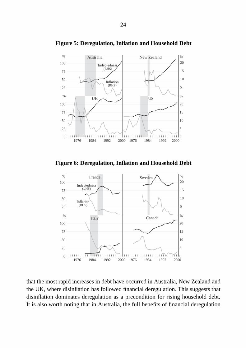
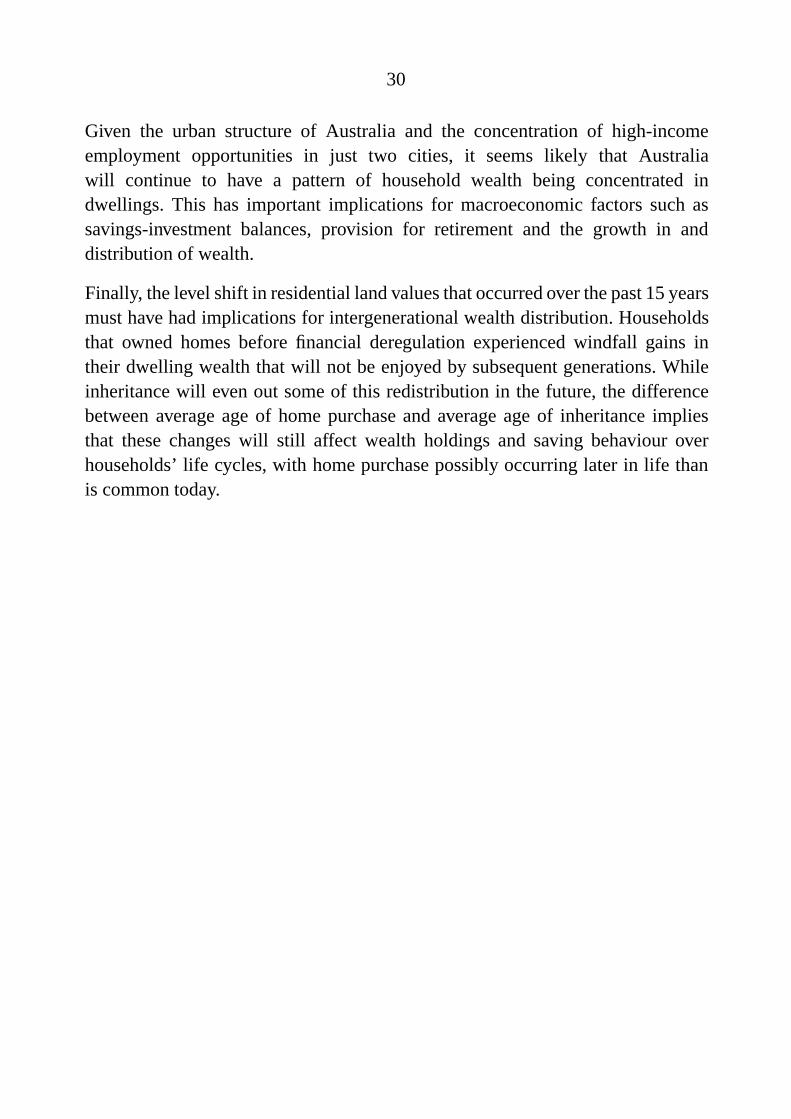
When the financial sector is regulated, credit is rationed and households cannotborrow as much as they would like at the current interest rate.16 Once theseconstraints are removed, household indebtedness usually rises, as shown inFigures 5 and 6 for eight countries; the period where deregulation took place,marked by a grey band, is frequently followed by a rapid increase inindebtedness.17 By contrast, Canada has always had a fairly deregulated homeloan market (Edey and Hviding 1995; Freedman 1998), and never experienced therapid run-up in debt seen in Australia, New Zealand, Sweden or the UK, whichreflected pent-up demand following the removal of restrictions.

Some of the increase in indebtedness may have been due to existing home ownerswithdrawing housing equity, for example by refinancing and increasing theirmortgages or by taking out a home equity loan. Households could also withdrawequity indirectly, for example if a household that inherits a house that was ownedoutright sells it to a household that took out a mortgage to make the purchase,and either consumes the proceeds or channels them into non-housing assets.This would result in higher consumption but not necessarily higher dwellingprices. Still, the removal of credit constraints on mortgage borrowers enablessome households who previously did not own a home to purchase one, and someexisting home owners to upgrade to a better home. This should be expected toresult in increased effective demand for owner-occupied housing and thereforeupward pressure on dwelling prices.

The rapid build-up in household indebtedness, however, appears to be moreclosely associated with a reduction in inflation to low levels. Figures 5 and 6 show

16 Duca and Rosenthal (1994) found that borrowing constraints lowered the US owner-occupationrate by around 8 percentage points, disproportionately affecting young households.

17 Appendix B contains the sources we used to construct the dates of the period of financialderegulation in each country.

24

Figure 5: Deregulation, Inflation and Household Debt

0

25

50

75

100

25

50

75

100

5

10

15

20

0

5

10

15

20

2000

%

(LHS)Indebtedness

199219841976 1976 1984 1992 2000

Inflation(RHS)

Australia %

USUK

New Zealand

%

%

Figure 6: Deregulation, Inflation and Household Debt

0

5

10

15

20

0

25

50

75

100

5

10

15

20

25

50

75

100

%

(RHS)

Indebtedness

%

%%Canada

2000199219841976 1976 1984 1992 2000

Inflation

(LHS)

France Sweden

Italy

that the most rapid increases in debt have occurred in Australia, New Zealand andthe UK, where disinflation has followed financial deregulation. This suggests thatdisinflation dominates deregulation as a precondition for rising household debt.It is also worth noting that in Australia, the full benefits of financial deregulation

25

did not accrue to households until the 1990s, with financial intermediaries mainlydirecting their lending toward businesses in the 1980s (Stevens 1997).

Even with a deregulated financial sector, high inflation will still constrainhousehold debt because some imperfections and information asymmetries remain.Mortgage contracts are usually based on regular repayments fixed in nominalterms. Given this, financial institutions will only lend to households as muchas they can reasonably service on their current incomes; in Australia, mostfinancial intermediaries impose a maximum loan size corresponding to arepayment-to-income ratio of around 30 per cent. It is the nominal interest rate,not the real rate, that determines this repayment ratio. Therefore the higher isinflation, and thus the higher are nominal rates, the more households are affectedby this market imperfection and excluded from the home loan market (Lessardand Modigliani 1975; Stevens 1997). Disinflation will therefore unambiguouslyincrease demand for owner-occupied housing, although this effect may have beendampened in countries such as the United States, where mortgage interest isdeductible. Existing home owners will be able to upgrade, current renters willbe more likely to be able to move into home ownership, and new households mayform as an endogenous response to the reduced costs of mortgage finance.18 Thisincreased the effective demand for housing, resulting in higher housing prices anda relatively static home-ownership rate.

Deregulation and disinflation certainly affected household debt, but it did notnecessarily follow that dwelling wealth-income ratios increased in all countries.Growth in dwelling wealth after deregulation and disinflation largely reflects thedifference between its actual level in the regulated period and its putative desiredlevel. The relationship between the actual and desired level was determined by theextent to which distortions in the housing market offset the effects of high inflationand financial regulation. We have already seen that these policies were not uniformacross countries (see Table 3). In the presence of credit constraints, mortgageinterest deductibility and capital gains exemptions on the family home in the UKand US made dwellings very attractive relative to other investments. This mayhave worked to offset the effects of regulation and thus closer align actual dwelling

18 Poterba (1984) suggests that the interaction between inflation and mortgage interestdeductibility could have explained the strong growth in US house prices during the 1970s.However, demographic factors such as the entry of the baby-boom generation into itshouse-buying years have also been cited as a potential cause (Mankiw and Weil 1989).

26

wealth with its desired level. Furthermore, mortgage interest deductibility in theUK and US would have ameliorated the burden that high inflation placed onmortgage borrowers; Britten-Jones and McKibbin (1989) found that changes inmortgage interest deductibility have a much larger effect on the housing marketthan changes in income taxes. These factors combined to mean that the actuallevel of dwelling wealth under regulation was possibly closer to its desired levelthan was the case in Australia.19 That dwelling wealth-income ratios in the US andUK are currently around their 1980 level is consistent with this point (see Table 2).

Fewer housing market distortions in Australia and New Zealand made the relativeconstraint placed on dwelling wealth by high inflation and financial regulationmore binding. These constraints seem to have disproportionately affected citiesthat would otherwise have had high housing costs. The suppression of this urbanstructure effect widened the gap between actual dwelling wealth and its desiredlevel. It took financial deregulation and disinflation to release this effect, and sincethen dwelling prices have responded accordingly, with the largest increases seen inSydney and more recently Melbourne. It is therefore possible that national averagedwelling wealth has been able to rise to its long-run level, now that housingprices in these cities are no longer constrained by these regulations. This mayexplain why Australia’s dwelling wealth-income ratio has increased relative toother countries, from around the international average to well above it.

On the other hand, if the combined effects of high inflation and financial regulationhad kept housing prices artificially low, they may also have had an effect on thecurrent composition of the dwellings stock. These constraints on purchase priceswould have affected building costs very little, so most of the effect would havemanifested in land prices. Although home buyers may have been constrainedfrom paying as much as they would in a deregulated environment, the artificiallylow land prices might have allowed inframarginal home buyers to purchase ahigher-quality home than they would if prices had been higher. In particular,they might have been able to purchase a home that used more land. This mightgo some way to explaining the greater prevalence of detached houses in theAustralian housing stock which, as alluded to in Section 2.2, might indicate a

19 In the UK, some of this incentive would have been undermined by the existence of a largepublic-housing sector. Pent-up demand for dwellings was unleashed in the late 1980s whensome public housing was privatised (Henley 1999).

27

more land-intensive component to past demand for new housing than occurred inother countries.

Because the stock of housing greatly exceeds the flow of new building, it takes along time for the characteristics of the stock to adjust to structural change suchas a new post-deregulation equilibrium price. Therefore although the equilibriumprice of housing may have risen following these changes, the aggregate valueof the housing stock might be above its long-run level because the compositionof the housing stock is yet to adjust fully. Now that land prices are no longerheld down by inflation and financial regulation, people will tend to choose lessland-intensive housing than in the past, supporting the trend to medium-densityhousing, especially in the larger cities.

5. A Two-factor Model of City Populations

As discussed by Krugman (1996), models generating power laws for their sizedistributions generally involve the interplay of a centripedal force encouragingpopulation into large agglomerations, balanced by a centrifugal force such ascongestion costs, that limits this tendency to agglomeration. In this section, weoutline a simplified model that generates Zipf’s Law for some parameter values,primate cities for others, and flat rank-size relationships similar to that in Australiafor others.20 Although this model clearly excludes some important details ofthe evolution and growth of cities, it captures some essential features that maygenerate insights about the forces driving both the urban structure and relativehousing costs seen in Australia.

The household location decision involves a trade-off in which households comparethe employment benefits that large cities offer, against the increased costs ofcongestion, proxied by high dwelling prices. In our model, two types of firmsdemand labour: local and national firms. Local firms sell only into the city marketthey are in, and compete only with other firms in that city. The number of suchfirms is random but roughly proportional to city populations. National firms onthe other hand sell into the entire national market and locate so as to minimisetransport and land costs. This creates a tendency for national firms to locate inthe largest city and fosters the formation of large agglomerations, although this

20 The details of the model are provided in Appendix A.

28

is partly offset by land costs which we proxy by housing costs. However, thesize of cities is constrained by housing costs, which rise with population size.Since households prefer to minimise commuting times, they are willing to pay apremium to live close to the city centre. This tends to raise housing prices as thecity grows, discouraging the formation of large agglomerations.

The relative importance of these two effects depends upon two key parameters:the share of national firms in the economy (β) and transport costs (θ). Our modelassumes the birth rate in city i is a random variable that has a common varianceacross cities and a mean that is scaled by attractiveness of that city relative tothe national average of all cities. For each pair of values for the parameters βand θ, we conduct 500 simulations, each of 500 periods for a country of 100cities. When the share of national firms is small, we can generate rank-sizerelationships consistent with Zipf’s Law. However, as β and θ rise, the Zipf curvetends to flatten as the largest city commands an increasing share of the populationand the national average house price rises. This distinguishes our model fromprevious random growth models which could only generate city size distributionsconsistent with Zipf’s Law, and not deviations from it. Moreover, our modelof city formation captures the Australian experience: countries with relativelysmall populations (high β) spread over large distances (high θ) will have moreconcentrated populations and higher average housing costs than countries withoutthese characteristics.

6. Conclusion

Economic researchers have long recognised the potential for demographic factorsto drive medium-term outcomes in the labour market and financial asset returns.This paper argues that spatial aspects of demography are important for the level ofnon-financial wealth and housing costs. We argue that Australia’s flat Zipf curveis a result of its federal political system and sparse population, which interactto produce multiple primate cities. The relationship between these primate citiesarises because some serve as national centres to a greater extent than others, andtherefore attract relatively more population from the small towns than do thesmaller primate cities (state capitals).

The link from urban structure to average dwelling prices is more subtle. Giventhat large cities have higher housing costs, the argument that national average

29

dwelling prices will be higher in countries with a larger share of their populationconcentrated in large cities would seem to be a matter of arithmetic. However,this cannot be the only explanation of the pattern of Australia’s household wealth– otherwise, we would see Canada’s wealth having a similar composition andGermany’s less similar. Sweden would have had a much higher share of dwellingwealth had it not been for its large public and co-operative sectors holding marketdwelling prices down.

If our arguments about the link between urban structure and national averagedwelling prices are right, we would expect that dwelling wealth will be higherrelative to income in Australia than in other countries, in the long run. This impliesthat housing debt-income ratios could be higher in equilibrium in Australia thanelsewhere, without this being a cause for concern. If so, the rapid build-up ofhousing indebtedness over the 1990s may still have some way to go. Nonetheless,growth in housing prices and debt will still have to level out at some stage, to matchnominal income growth in the long run. As has already occurred in New Zealand,the windfall gains that accrued to home owners over the 1980s and 1990s willultimately end.

However, our estimate of the effect of urban structure on dwelling wealth accountsfor only one-third – or at best, one-half – of the gap between Australian andUS dwelling wealth-income ratios. This may suggest that dwelling prices aretoo high in Australia and must ultimately fall relative to household income.Fortunately, the prospect of a sudden crash in dwelling prices similar to thatseen in the UK in the early 1990s seems remote. Australia’s unusually highdwelling wealth-income ratio has built up over fifteen years, not in a brief periodof speculation, and the specific circumstances that contributed to that boom-bustcycle do not apply here (Muellbauer 1992; Henley 1999; Bean 2000). It wouldseem more likely that such an adjustment would occur through an extended periodof slow or zero growth in dwelling prices, and perhaps partly through a shift in thecomposition of the dwelling stock towards higher-density homes rather than pricesof particular dwellings falling. Whether that adjustment caused financial distressin some segments of the household sector would depend on whether householdshad over-extended themselves, in the erroneous belief that dwelling prices wouldcontinue to grow strongly.

30

Given the urban structure of Australia and the concentration of high-incomeemployment opportunities in just two cities, it seems likely that Australiawill continue to have a pattern of household wealth being concentrated indwellings. This has important implications for macroeconomic factors such assavings-investment balances, provision for retirement and the growth in anddistribution of wealth.

Finally, the level shift in residential land values that occurred over the past 15 yearsmust have had implications for intergenerational wealth distribution. Householdsthat owned homes before financial deregulation experienced windfall gains intheir dwelling wealth that will not be enjoyed by subsequent generations. Whileinheritance will even out some of this redistribution in the future, the differencebetween average age of home purchase and average age of inheritance impliesthat these changes will still affect wealth holdings and saving behaviour overhouseholds’ life cycles, with home purchase possibly occurring later in life thanis common today.

31

Appendix A: A Model of City Formation and Dwelling Prices

Cities

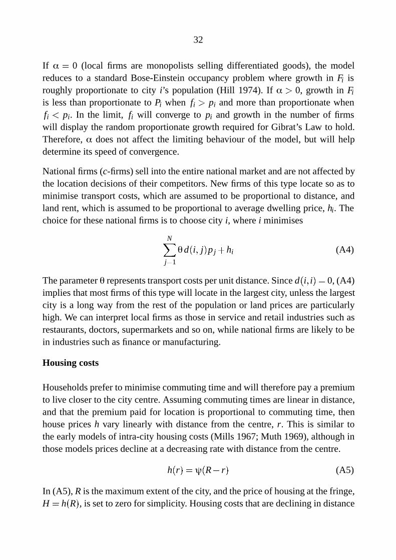
There are N cities, with city i located at position li having population Pi andshare of total population pi � Pi�P where P �Pi Pi. The cities are randomlyplaced around a circle, implying 0 � li � 2π. This simplifies the analysis whileat the same time being a reasonable approximation of Australia’s geography. Thedistance between cities is therefore:

d�i� j� � min�jli� l jj� j2π� li� l jj� (A1)

For the purpose of this paper, we assume that city locations are fixed. However, itmay be possible to use models such as Krugman’s (1996) to extend our model toallow city locations to be endogenous. We leave this task to future research.

Firms

There are two types of firm, local and country-wide.21 Firms are of equal size,with the number and share of local firms in city i denoted Fi and fi, and similarlyCi and ci for national (country-wide) firms. We denote the share of national firmsin total firms as β.

β� CF �C

(A2)

Local firms ( f -firms) sell only into the city market they are in, and compete onlywith other firms in that city. Therefore their location decisions are driven by therelative size (population share) of each city, and also influenced by the number oflocal firms already in that city. The probability that a new local firm will choose tolocate in city i is assumed to be proportional to:�

pi

fi

�α� pi, 0� α� 1 (A3)

where α is an index of the intensity of competition or substitutability of the newfirms’ output with the output of firms already in city i.

21 This distinction is a variant of the approach taken by the existing literature. For instance,Krugman (1996) assumes two sectors: a geographically immobile sector (agriculture)and an increasing returns, monopolistically competitive, geographically mobile sector(manufacturing).

32

If α � 0 (local firms are monopolists selling differentiated goods), the modelreduces to a standard Bose-Einstein occupancy problem where growth in Fi isroughly proportionate to city i’s population (Hill 1974). If α � 0, growth in Fi

is less than proportionate to Pi when fi � pi and more than proportionate whenfi � pi. In the limit, fi will converge to pi and growth in the number of firmswill display the random proportionate growth required for Gibrat’s Law to hold.Therefore, α does not affect the limiting behaviour of the model, but will helpdetermine its speed of convergence.

National firms (c-firms) sell into the entire national market and are not affected bythe location decisions of their competitors. New firms of this type locate so as tominimise transport costs, which are assumed to be proportional to distance, andland rent, which is assumed to be proportional to average dwelling price, hi. Thechoice for these national firms is to choose city i, where i minimises

NXj�1

θd�i� j�pj�hi (A4)

The parameter θ represents transport costs per unit distance. Since d�i� i� � 0, (A4)implies that most firms of this type will locate in the largest city, unless the largestcity is a long way from the rest of the population or land prices are particularlyhigh. We can interpret local firms as those in service and retail industries such asrestaurants, doctors, supermarkets and so on, while national firms are likely to bein industries such as finance or manufacturing.

Housing costs

Households prefer to minimise commuting time and will therefore pay a premiumto live closer to the city centre. Assuming commuting times are linear in distance,and that the premium paid for location is proportional to commuting time, thenhouse prices h vary linearly with distance from the centre, r. This is similar tothe early models of intra-city housing costs (Mills 1967; Muth 1969), although inthose models prices decline at a decreasing rate with distance from the centre.

h�r� � ψ�R� r� (A5)

In (A5), R is the maximum extent of the city, and the price of housing at the fringe,H � h�R�, is set to zero for simplicity. Housing costs that are declining in distance

33

from the centre fit in with the von-Thunen-Mills models of land rent and allocationaround a central place (Mills 1967). If the city is circular, its area – equivalently,population or number of dwellings – is Pi � πR2. There are 2πr dwellings at radiusr. Therefore the city’s average housing price, hi varies with the square root of itspopulation.

hi �

R R0 h�r�2π r dr

πR2 �ψR Pi

0

pPi�a da

Pipπ

�ψp

Pi

3pπ

(A6)

This functional form depends on the assumption of a fixed floor for housing prices;prices at the very fringe of the city do not depend on the size of the city. Itis also possible that commuting times will vary more than proportionately withdistance from the centre, due to congestion. Alternatively, the development ofedge cities and increasing prevalence of employment opportunities in the suburbscould mean that congestion costs rise less than proportionately with population(Krugman 1995). However, this will not reverse the central result that averagehousing prices are higher in larger cities, and that national average housing pricesare higher when the population is concentrated in a few centres. In the simulationsbelow, we define hi as

pPi, effectively setting the scaling factor ψ to 3

pπ.

Household location decisions

We assume a city’s attractiveness to households depends on three factors: theavailability of jobs, the absolute population of the city and the average level ofhousing costs. We measure the availability of jobs by ��1� β� fi � β ci��pi. Thedirect inclusion of city populations is intended to account for the observed wagepremium seen in larger cities (Glaeser and Mare 2001). This may reflect eitherthat search costs are lower in larger labour markets, or that larger markets allowfor greater specialisation, which raises wages. In addition, larger cities have morediverse industrial structures and thus may be attractive locations to a wider rangeof workers (Gabaix 1999b).

Housing costs work against these forces encouraging greater agglomeration.Although there may be other disadvantages to living in large cities, such ascongestion, pollution and crime, we take housing costs as a proxy for all of thesecosts, given that they are monotonic in city population. Since the attractivenessof a city, u��� represents the utility it offers to its residents, we assume that it

34

has a fairly standard functional form, the Cobb-Douglas function. This ensuresdeclining marginal utility of absolute city size.

ui ��

u��1�β� fi�β cipi

�Pi�hi�����1�β� fi�β ci

pi

�λP1�λ

i h�µi , 0 � λ�µ � 1 (A7)

Following Gabaix (1999a), we assume that in each period t, gt P new householdsare born and δP households die; the death rate δ is constant across time and acrosscities.22 Total births nationwide are random, with the growth rate gt distributedlognormally with mean γ and a variance that depends on σ2. The allocation ofnew households to cities is determined by the attractiveness of that city relative tothe national average of all cities. This relative attractiveness is scaled so that theirweighted sum equals one. Suppressing the time subscripts, we have:

U�i� � ui�

NXj�1

p j u j (A8)

We define the birth rate in city i, gi t as a lognormal random variable with commonvariance σ2 and a mean that is scaled by the relative attractiveness of that city inthat period. The scaling factor used in the definition of relative attractiveness (A8)ensures that the mean growth rate for the total population equals γ.

git � γU�i�t (A9)

Importantly, we do not assume that all (new) households move to whichever is themost attractive city, as this would result in the system having unstable dynamics.Depending on the relative importance of housing costs versus employmentopportunities, either the largest city would then increase without limit while theother cities fade away at rate δ, or the smallest, cheapest, city would attract allthe new population and become large. If the smallest city attracts the population,it is then no longer the most attractive city, and the city that had previouslybeen the second-smallest attracts all the new population in the following period.The functional forms for the utility and housing-price relations used here resultin the net effect of rising population on its relative attractiveness varying withP1�λ�µ�2

i . If 1� λ is very different from µ�2, the (unbounded) city populationeffect dominates the effect of job availability in the long run. This does not

22 We assume that each household contains one person.

35

materially distort the simulation results presented below, as the net effect of citypopulation remains fairly small for the range of populations considered.

By contrast, allowing random growth in all cities captures the reality of theprocess of birth or household formation, while allowing households to respondto economic forces by having some change location. Random growth with a meandepending on economic factors effectively captures moving costs – it is not alwaysadvantageous to move to the most attractive city – and unobserved heterogeneity –not everyone will want to move even if it would benefit the median new household.Alternatively, these costs and individual variation could be modelled, but onlyby adding many free parameters and functional forms without much theoreticalguidance to pin them down. In our view, this would add complexity to the modelwithout adding much explanatory power.

One final adjustment is required to prevent city populations from being zero. Theactual increase in population in each city is defined as:

Pit �Pit�1 � gi tPi t�1�δPit�1� ε (A10)

where ε is a small positive number which we set equal to 1. Gabaix (1999b)showed that random proportionate growth with a lower bound on population,which he termed a Kesten process, will generate Zipf’s Law in the upper tail of asize distribution.

Simulation results

The results in this Appendix are based on an extensive exploration of the modelfor a range of parameters. For each pair of values for the parameters β and θ, weconducted 500 simulations, each of 500 periods for a country of 100 cities. The αparameter does not affect the long-run results, so we set it to 0�5 throughout. Themean birth rate γ was set to 0�03 and the death rate δ to 0�02. The parameters in thehousehold utility function are λ� 0�9 and µ � 0�15, so large cities are on balancemore attractive than smaller ones even when the labour market in each city is inequilibrium. Similar results are obtained within a significant neighbourhood ofthese parameter values. The figures below show the median final-period outcomeand the 5th and 95th percentile of those 500 cases, for dwelling prices, thelargest city’s share of the total population and the slope of the ‘Zipf curve’, orlog rank-log size relationship, for the top 50 cities. We find that the rank-size

36

relationship tends to flatten out after this point. This is in line with the findingthat random growth generates Zipf’s Law in the upper tail of the distribution,but not necessarily for the whole sample (Gabaix 1999b; Hill 1974); a simpleKesten process as in Equation (A10), where git is a random variable drawn froma common distribution, will generate a Zipf curve with a linear segment coveringabout half to two-thirds of the sample.

If the share of national firms in the economy β is small, say, less than about0�05, our model generates rank-size curves roughly consistent with Zipf’s Law(Figure A1). As β rises, the simulations tend to generate flatter Zipf curves, withslopes around 0�5–0�7. With β above about 0�4, a primate city is almost guaranteed(Figure A2).

Figure A1: Simulation Results – Zipf Curve Slope50 largest cities

-2.0

-1.5

-1.0

-0.5

-2.0

-1.5

-1.0

-0.5

-2.0

-1.5

-1.0

-0.5

-2.0

-1.5

-1.0

-0.5

0.0

-2.0

-1.5

-1.0

-0.5

0.0θ = 10

0.02 0.10 0.20 0.30 0.40 0.10 0.20 0.30 0.40

θ = 100

θ = 1 000 θ = 10 000

β (share of national firms)

Zip

f cu

rve

slop

e Zipf curve slope

Median

95th percentile

5th percentile

As expected, increasing importance of national firms (β) and transport costs (θ)both result in the largest city having a larger share of total population. FlatterZipf curves and large primate cities imply higher national average dwelling prices(Figure A3). This seems in line with Australia’s situation: countries with relativelysmall populations (high β) spread over large distances (high θ) will have moreconcentrated populations and higher average housing costs than countries withoutthese characteristics.

37

Figure A2: Simulation Results – Share of Largest City

0.0

0.2

0.4

0.6

0.8

0.0

0.2

0.4

0.6

0.8

0.0

0.2

0.4

0.6

0.8

0.0

0.2

0.4

0.6

0.8

0.0

0.2

0.4

0.6

0.8

1.0

0.0

0.2

0.4

0.6

0.8

1.0

β (share of national firms)

θ = 10

0.02 0.10 0.20 0.30 0.40 0.10 0.20 0.30 0.40

θ = 100

θ = 1 000 θ = 10 000

Shar

e of

larg

est c

ityShare of largest city

Figure A3: Simulation Results – National Average Dwelling Prices

00 00

00

β (share of national firms)

θ = 10

0.02 0.10 0.20 0.30 0.40 0.10 0.20 0.30 0.40

θ = 100

θ = 1 000 θ = 10 000

3 000

2 000

1 000

3 000

2 000

1 000

2 000

1 000

2 000

1 000

Dw

ellin

g pr

ice D

welling price

The model we have used is not a complete model of city formation. In particular,we have left many stylised features of the economics of cities as exogenousfactors, such as the wage premium paid in large cities. The location decisionsof households and firms are assumed to depend only on current-period payoffs. Ina more complex model, agents would be forward-looking instead of myopic, butas Neary (2001) argues, and Baldwin (1999) demonstrates for the core-periphery

38

model, this added complexity does not affect the model’s comparative-staticspredictions. We also generated the higher housing costs in larger cities observedin Section 2.3 by geographic construction; a more sophisticated model wouldallow residents to respond to housing costs by endogenously adjusting thesize and quality of new dwellings. Although random birth of households isbiologically justifiable, the random allocation of local firms ( f -firms) is lessjustifiable on economic grounds. Recent research has developed models that canexplain these features as endogenous outcomes of microeconomic behaviour, atthe cost of considerable extra complexity and computational burden (Axtell andFlorida 2001). Nonetheless, our model illustrates that a few simple variations on arandom-growth model can generate rank-size distributions that match the data fora range of countries reasonably well.

39

Appendix B: Data Sources

Population

For Australia, Australian Demographic Statistics, ABS Cat No 3101.0(March 2000 release). Population of all towns and cities with more than4 900 inhabitants from the 1996 Census, available at <URL:http://www.abs.gov.au>. For Canada, data are estimates for 1999, taken from the StatisticsCanada website, available at <URL:http://www.statcan.ca/english/Pgdb/People/Population/demo05.htm>. For New Zealand, data are from the 1996 Census(Statistics New Zealand). For the United States, MSA and CSMA population datafor 1999 were taken from the Bureau of Census website, available at <URL:http://www.census.gov>. For all other countries, city population data from theUnited Nations Statistics Division Population Database, available at <URL:http://www.un.org/Depts/unsd/demog/ctry.htm>.

Table 3

Mortgage interest deductibility: OECD (1994).

Capital gains tax exemption: OECD (1994).

Share of public housing: Australia [1999]: Australian Social Trends, ABSCat No 4102.0; Canada: Statistics Canada website; France, Germany, Italy,Sweden, United Kingdom: European Parliament (1996); Japan [1998]:1998 Housing and Land Survey of Japan, Statistics Bureau and StatisticsCenter; New Zealand: Statistics New Zealand [1996 Census] and Ministryof Housing; United States [1997]: authors’ calculation based on the numberof public housing units reported by the US Department of Housing andUrban Development and the total housing stock from American HousingSurvey 1999.

Home ownership rates: Australia [1999]: ABS Cat No 4102.0. Canada: StatisticsCanada [Census and related data 1999]; France [1996], Germany [1998],Italy [1991], United Kingdom [1998]: Haffner and Dol (2000); Japan[1998]: Housing of Japan, Statistics Bureau and Statistics Center; Sweden:Oswald (1999); New Zealand [1996]: Statistics New Zealand [1996Census]; United States [1999]: US Census Bureau.

40

Table 4

Persons per room: United Nations Statistics Division, available at <URL:http://www.un.org/Depts/unsd/social/housing.htm>.

Average existing dwelling size: Australia: authors’ calculation based on floorspace per person for Melbourne from the USAID Housing IndicatorsProject [1993] and persons per household from ABS Cat No 4102.0;Canada [1985]: Canada Mortgage and Housing Corporation; France[1996], Germany [1998], Italy [1985], Sweden [1997]: Haffner andDol (2000); Japan [1998]: 1998 Housing and Land Survey of Japan,Statistics Bureau and Statistics Center; New Zealand [mid 1990s]:Valuation New Zealand Sales Data as cited in Bourassa and Hoesli (1999);United Kingdom: English House Condition Survey 1996, Department ofEnvironment, Transport and the Regions; United States [1997]: AmericanHousing Survey 1999, Census Bureau.

Average new dwelling size: Australia [1999]: ABS Cat No 4102.0; France[1998], Germany [1999], Italy [1996], Sweden [1998], United Kingdom[average 1980–1996]: Haffner and Dol (2000); Japan [1998]: 1998 Housingand Land Survey of Japan, Statistics Bureau and Statistics Center; UnitedStates [1999]: National Association of Home Builders.

Proportion of dwellings houses: Australia [1998]: ABS Cat No 4102.0; Canada:Statistics Canada [Census and related data 1999]; France [1996], Germany[1998], Sweden [1998]: Haffner and Dol (2000); New Zealand [1996]:Statistics New Zealand; United Kingdom [1996]: English House ConditionSurvey; United States [1997]: American Housing Survey 1999.

Proportion of dwellings detached: Australia [1998]: ABS Cat No 4102.0;Canada: Statistics Canada [Census and related data 1999]; Germany[1997]: Miron (2001); Japan [1993]: Building Council of Japan (1998);New Zealand [mid 1990s]: Valuation New Zealand Sales Data as citedin Bourassa and Hoesli (1999); United Kingdom [1996]: English HouseCondition Survey; United States [1997]: American Housing Survey 1999.

41

Dwellings with six or more rooms: Australia [1999]: Australian Housing Survey,ABS Cat No 4182.0; Canada [1996], France [1996], Germany [1997],United Kingdom [1996/97], United States [1997], New Zealand [1996]:Miron (2001).

Dwellings built since 1980: Australia: authors’ calculation based on Census dataand building completions (ABS Cat No 8752.0); France [1996], Germany[1998], Sweden [1990], United Kingdom [1996]: Haffner and Dol (2000);Japan [1998]: 1998 Housing and Land Survey of Japan, Statistics Bureauand Statistics Center; United States [1997]: American Housing Survey1999.

Figure 1, Table 5, Table 7 and Table 8: Actual and Counterfactual DwellingPrice-Income Ratios

Australian housing prices by city: CBA/HIA Housing Report and, for Hobart,Real Estate Institute of Australia. The data in Figure 1 are for December2000. The data in Tables 5, 7 and 8 are for June 1998.

Australian median household gross income by city: ABS Household ExpenditureSurvey 1998-1999 (median income provided as a special data service). InFigure 1, income is deflated by national accounts gross household income(ABS Cat No 5206.0).

Australian average household disposable income: National Income, Expenditureand Product, (ABS Cat No 5206.0). The number used is an average ofquarterly data for 1998.

US housing prices by city: National Association of Realtors, available at <URL:http://nar.realtor.com/databank/ehsmet.htm>.

US national average housing prices: Mylonas et al (2000).

US median household gross income by city: Census Bureau Current PopulationSurvey, Small Area Income and Poverty Estimates for 1997, available at<URL:http://www.census.gov/hhes/www/saipe/stcty/estimate.html>.

42

US average household disposable income: Survey of Current Business May2000, Table 2.1, Bureau of Economic Analysis, Department of Commerce;US Census Bureau Household and Housing Unit Estimates 1998,available at <URL:http://www.census.gov/population/estimates/housing/sthuhh1.txt>.

Figures 5 and 6: Dates of Financial Deregulation

The dates of financial deregulation correspond to the period when interest rateceilings on deposits and loans, and quantitative restrictions on bank lending werelifted in each country.

Australia: Battellino and McMillan (1989).

Canada: Edey and Hviding (1995); Freedman (1998); Germany andMorton (1985); OECD (2000).

France, Italy and Sweden: OECD (2000).

New Zealand: OECD (2000); Margaritis, Hyslop and Rae (1992).

United Kingdom: Germany and Morton (1985); OECD (2000).

United States: Edey and Hviding (1995); Jaffee and Stiglitz (1990); Mehrez andKaufmann (1999).

43

References

Ades AF and EL Glaeser (1995), ‘Trade and Circuses: Explaining Urban Giants’,Quarterly Journal of Economics, 110(1), pp 195–227.

Axtell RL and R Florida (2001), ‘Emergent Cities: A MicroeconomicExplanation of Zipf’s Law’, paper presented at 7th International Conference ofthe Society for Computational Economics, Yale, June.

Baldwin RE (1999), ‘The Core-Periphery Model with Forward-LookingExpectations’, Centre for Economic Policy Research Discussion Paper No 2085.

Battellino R and N McMillan (1989), ‘Changes in the Behaviour of Banks andtheir Implications for Financial Aggregates’, Reserve Bank of Australia ResearchDiscussion Paper No 8904.

Bean C (2000), ‘The Australian Economic “Miracle”: A View from the North’, inD Gruen and S Shrestha (eds), The Australian Economy in the 1990s, Proceedingsof a Conference, Reserve Bank of Australia, Sydney, pp 73–114.

Bourassa SC and M Hoesli (1999), ‘The Structure of Housing Submarkets in aMetropolitan Region’, University of Aberdeen Working Paper No 99-4.

Bourassa SC and PH Hendershott (1992), ‘Over-investment in Australianhousing?’, National Housing Strategy Background Paper No 9.

Britten-Jones M and WJ McKibbin (1989), ‘Tax Policy and Housing Investmentin Australia’, Reserve Bank of Australia Research Discussion Paper No 8907.

Building Council of Japan (1998), A Quick Look at Housing in Japan, 4th edn,Building Council of Japan, Tokyo.

Cardew R, A Parnell and B Randolph (2000), ‘Sydney Housing AffordabilityReview’, University of Western Sydney Urban Frontiers Program IssuesPaper No 3.

Duca JV and SS Rosenthal (1994), ‘Borrowing constraints and accessto owner-occupied housing’, Regional Science and Urban Economics, 24,pp 301–322.

44

Edey M and K Hviding (1995), ‘An Assessment of Financial Reform in OECDCountries’, OECD Economics Department Working Paper No 154.

European Parliament (1996), ‘Housing Policy in the EU Member States’, TheEuropean Parliament, Directorate General for Research Social Affairs Series NoW14.

Freedman C (1998), ‘The Canadian Banking System’, Bank of Canada TechnicalReport No 81.

Gabaix X (1999a), ‘Zipf’s Law and the Growth of Cities’, American EconomicReview, 89(2), pp 129–132.

Gabaix X (1999b), ‘Zipf’s Law for Cities: An Explanation’, Quarterly Journal ofEconomics, 114(3), pp 739–767.

Germany JD and JE Morton (1985), ‘Financial Innovation and Deregulation inForeign Industrial Countries’, Federal Reserve Bulletin, 71(10), pp 743–753.

Girouard N and S Blondal (2001), ‘House Prices and Economic Activity’,OECD Economics Department Working Paper No 279.

Glaeser EL and DC Mare (2001), ‘Cities and Skills’, Journal of LaborEconomics, 19(2), pp 316–342.

Haffner MEA and CP Dol (2000), Housing Statistics in the European Union2000, OTB Research Institute for Housing, Urban and Mobility Studies, DelftUniversity of Technology.

Henderson JV (1974), ‘The Sizes and Types of Cities’, American EconomicReview, 64(4), pp 640–656.

Henderson JV and YM Ioannides (1983), ‘A Model of Housing Tenure Choice’,American Economic Review, 73(1), pp 98–113.

Henley A (1998), ‘Changes in the Distribution of Housing Wealth in Great Britain,1985–91’, Economica, 65(259), pp 363–380.

Henley A (1999), ‘The Economics of the Crazy British Housing Market’,Aberystwyth University Economic Research Paper No 99/8.

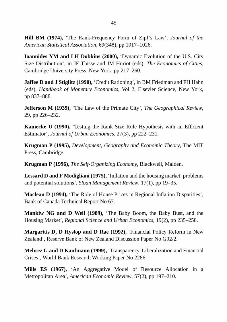
45

Hill BM (1974), ‘The Rank-Frequency Form of Zipf’s Law’, Journal of theAmerican Statistical Association, 69(348), pp 1017–1026.

Ioannides YM and LH Dobkins (2000), ‘Dynamic Evolution of the U.S. CitySize Distribution’, in JF Thisse and JM Huriot (eds), The Economics of Cities,Cambridge University Press, New York, pp 217–260.

Jaffee D and J Stiglitz (1990), ‘Credit Rationing’, in BM Friedman and FH Hahn(eds), Handbook of Monetary Economics, Vol 2, Elsevier Science, New York,pp 837–888.

Jefferson M (1939), ‘The Law of the Primate City’, The Geographical Review,29, pp 226–232.

Kamecke U (1990), ‘Testing the Rank Size Rule Hypothesis with an EfficientEstimator’, Journal of Urban Economics, 27(3), pp 222–231.

Krugman P (1995), Development, Geography and Economic Theory, The MITPress, Cambridge.

Krugman P (1996), The Self-Organizing Economy, Blackwell, Malden.

Lessard D and F Modigliani (1975), ‘Inflation and the housing market: problemsand potential solutions’, Sloan Management Review, 17(1), pp 19–35.

Maclean D (1994), ‘The Role of House Prices in Regional Inflation Disparities’,Bank of Canada Technical Report No 67.

Mankiw NG and D Weil (1989), ‘The Baby Boom, the Baby Bust, and theHousing Market’, Regional Science and Urban Economics, 19(2), pp 235–258.

Margaritis D, D Hyslop and D Rae (1992), ‘Financial Policy Reform in NewZealand’, Reserve Bank of New Zealand Discussion Paper No G92/2.

Mehrez G and D Kaufmann (1999), ‘Transparency, Liberalization and FinancialCrises’, World Bank Research Working Paper No 2286.

Mills ES (1967), ‘An Aggregative Model of Resource Allocation in aMetropolitan Area’, American Economic Review, 57(2), pp 197–210.

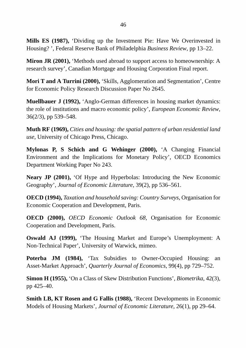
46

Mills ES (1987), ‘Dividing up the Investment Pie: Have We Overinvested inHousing? ’, Federal Reserve Bank of Philadelphia Business Review, pp 13–22.

Miron JR (2001), ‘Methods used abroad to support access to homeownership: Aresearch survey’, Canadian Mortgage and Housing Corporation Final report.

Mori T and A Turrini (2000), ‘Skills, Agglomeration and Segmentation’, Centrefor Economic Policy Research Discussion Paper No 2645.

Muellbauer J (1992), ‘Anglo-German differences in housing market dynamics:the role of institutions and macro economic policy’, European Economic Review,36(2/3), pp 539–548.

Muth RF (1969), Cities and housing: the spatial pattern of urban residential landuse, University of Chicago Press, Chicago.

Mylonas P, S Schich and G Wehinger (2000), ‘A Changing FinancialEnvironment and the Implications for Monetary Policy’, OECD EconomicsDepartment Working Paper No 243.

Neary JP (2001), ‘Of Hype and Hyperbolas: Introducing the New EconomicGeography’, Journal of Economic Literature, 39(2), pp 536–561.

OECD (1994), Taxation and household saving: Country Surveys, Organisation forEconomic Cooperation and Development, Paris.

OECD (2000), OECD Economic Outlook 68, Organisation for EconomicCooperation and Development, Paris.

Oswald AJ (1999), ‘The Housing Market and Europe’s Unemployment: ANon-Technical Paper’, University of Warwick, mimeo.

Poterba JM (1984), ‘Tax Subsidies to Owner-Occupied Housing: anAsset-Market Approach’, Quarterly Journal of Economics, 99(4), pp 729–752.

Simon H (1955), ‘On a Class of Skew Distribution Functions’, Biometrika, 42(3),pp 425–40.

Smith LB, KT Rosen and G Fallis (1988), ‘Recent Developments in EconomicModels of Housing Markets’, Journal of Economic Literature, 26(1), pp 29–64.

47

Stevens GR (1997), ‘Some Observations on Low Inflation and HouseholdFinances’, Reserve Bank of Australia Bulletin, October, pp 38–47.

Sutton J (1997), ‘Gibrat’s Legacy’, Journal of Economic Literature, 35(1),pp 40–59.

Urzua CM (2000), ‘A simple and efficient test for Zipf’s Law’, EconomicsLetters, 66(3), pp 257–260.

Weicher JC (2000), ‘Comment on Steven C. Bourassa and William G. Grigsby’s“Income Tax Concessions for Owner-Occupied Housing”’, Housing PolicyDebate, 11(3), pp 547–559.

Zipf G (1949), Human Behaviour and the Principle of Least Effort,Addison-Wesley, Reading.