CIS 522: Lecture 15

Generalization and overfitting03/05/20

Intro

What is generalization?● Learn from a training set, evaluate on a test set● Generalization gap: Difference between loss on training

set and test set

Why is it hard?

Class 1

Class 2

Which class is this?

No free lunch theoremTheorem: If an algorithm performs better than random search on some class of problems then it must perform worse than random search on the remaining problems

In other words: ● A superior black-box optimization strategy is impossible● If our feature space is unstructured, we can do no better than random● “A jack of all trades is a master of none”

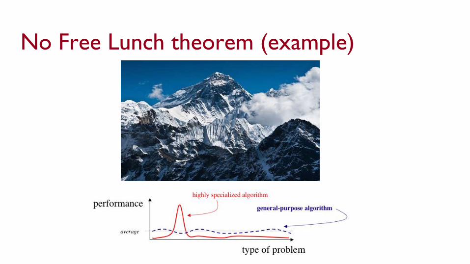
No Free Lunch theorem (example)

Overfitting

Overfitting

Generally if # parameters >> # data● More parameters means can fit more exactly● E.g. linear fit vs. higher degree polynomial

Why don’t neural networks overfit?

First answer: they do sometimes● Train for too long● Learning rate too small or batch size too large (will

explain later)● Training data doesn’t have easily learnable patterns

Memorization● Neural networks can learn random labels or random

input data● By definition, no generalization possible

“Understanding deep learning requires rethinking generalization”, Zhang et al., ICLR 2017

Meta-overfitting● Implicitly fitting algorithms to the test datasets

“Do ImageNet Classifiers Generalize to ImageNet?”, Recht et al., arXiv 2019.

Generalization before memorization● See work of Arpit et al. 2017● Neural nets performance on test set peaks before

performance on training set

Implicitly, we need inductive biases● E.g. towards lines and other “simple” functions● Towards spatially coherent objects in images● Can be hard to specify exactly what inductive biases are

right, but neural nets sometimes have them● Want to understand when nets will generalize and how

we can make them generalize better

Generalization guarantees

VC dimension● Suppose F is a set of functions● Say that F “shatters” a set of n data points if for every

possible labeling of the data points, there is some f in F that gets the labeling right

● The VC dimension of F is the maximum n such that F shatters all sets of n data points

● Intuitively: VC dim is size of sets that can be memorized

VC dimension● Ideally, we would want deep networks to have small VC

dimension - hard to memorize large amounts of data● But they have huge VC dimension: ≥ (# weights)2

● Still generalize pretty well!

Compressing networks● Can consider the effective size of networks instead● Many networks can be compressed to smaller networks

that perform just as well● Has been explored also in context of e.g. storing on

phones

How to compress a network● Train the network● Prune the low absolute-value weights● Re-train with those held at zero● Repeat● Can often remove ~90% of weights with negligible loss

of accuracy

PAC-Bayes with neural networks● Data-dependent bounds on generalization● Can get first non-trivial bounds - e.g. provable ~80% for

MNIST● Still not matching performance, but getting there● PAC framework: for small ε, δ > 0, draw function from

family F, prove only an ε chance of more than δ“Computing Nonvacuous Generalization Bounds for Deep (Stochastic) Neural Networks with Many More Parameters than Training Data”, Dziugaite and Roy, UAI 2016

Preventing overfitting

Regularization● Train to minimize normal loss + c * L1(weights)

○ Has the effect of driving some weights to 0○ See lasso regression

● Train to minimize normal loss + c * L2 (weights)○ Has the effect of making some weights small○ See ridge regression

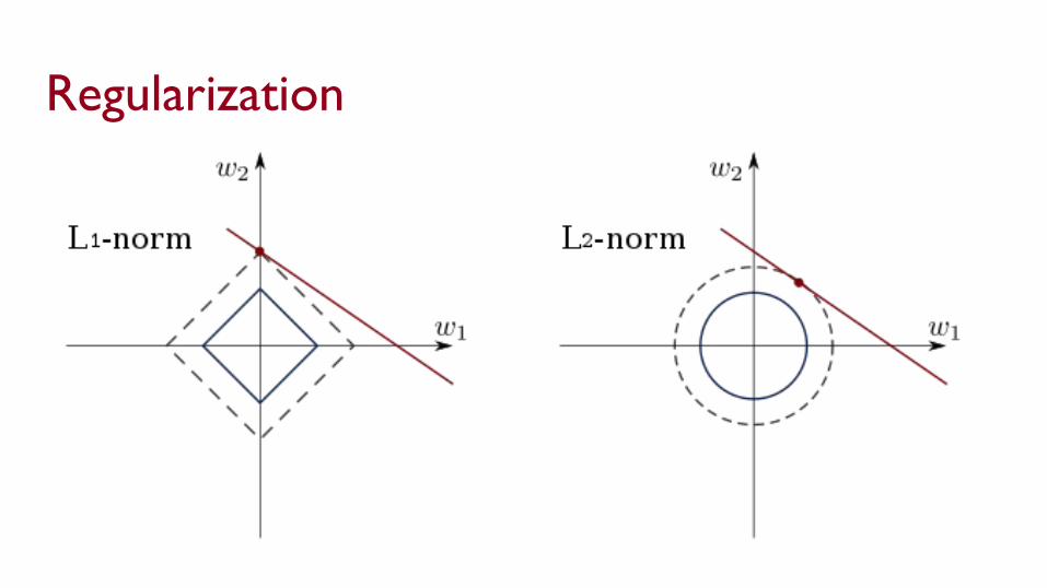
Regularization

Dropout● Recap: Kill some neurons during training time● Use all neurons during test time

Dropout● Prevents overfitting by breaking brittle predictions● Forces "dead branches" to learn● Enforces distributed nature● Distributes learning signal● Adds lots of noise● In a way approximates ensemble methods

Implicit regularization - ResNets

● Many paths for information flow through the network● No one path, or neuron, or layer, is necessary

Implicit regularization - ResNets

“Residual Networks Behave Like Ensembles of Relatively Shallow Networks”, Veit et al, NeurIPS 2016

Deep linear networks● No activation function:

Wk … W2 W1 x

● Seems kinda silly● Can express only linear functions (W = Wk … W2 W1 )

Implicit regularization - deep linear networks● But you are running backprop on many weight matrices

at once● Turns out to regularize!

Example: matrix completion (“Netflix prize”)● Given some entries of a matrix, try to complete the

matrix W, assuming it has low rank● Deep linear network: set W = Wk … W2 W1● Loss function: difference between predicted entries and

given entries + L2 norm of Wi● Proof: in certain cases, converges to W with min nuclear

norm (L1 norm of eigenvalues) (Gunasekar et al.)

Weird properties of large networks

Adversarial examples

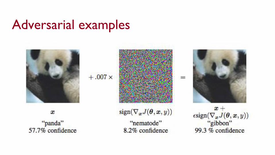
Adversarial examples

http://www.youtube.com/watch?v=piYnd_wYlT8

Adversarial examples● Inevitable consequence of learning in a high-dimensional

space?

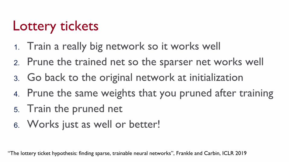
Lottery tickets1. Train a really big network so it works well2. Prune the trained net so the sparser net works well3. Go back to the original network at initialization4. Prune the same weights that you pruned after training5. Train the pruned net6. Works just as well or better!

“The lottery ticket hypothesis: finding sparse, trainable neural networks”, Frankle and Carbin, ICLR 2019

Lottery tickets

● If you knew the right weights to prune in advance, you wouldn’t need a massive network

● Suggests that a large network is an ensemble of many subnetworks - one of which got the “golden ticket” in the random initialization

“The lottery ticket hypothesis: finding sparse, trainable neural networks”, Frankle and Carbin, ICLR 2019

The optimization landscape

The optimization landscape● Shows how the loss varies as you vary the parameters● Essentially, graph of loss w.r.t. parameters● So 1M-dimensional if 1M parameters - hard to visualize

Local and global optima

Saddle points● Some parameter directions, loss goes up, some the loss

goes down

High-dimensional optimization● Since lots of possible directions, local minima actually

generally don’t occur for large networks● Lots of saddle points though

Real problem: flat areas● Flat area: most directions the loss stays roughly the

same● Problem because hard to get out of

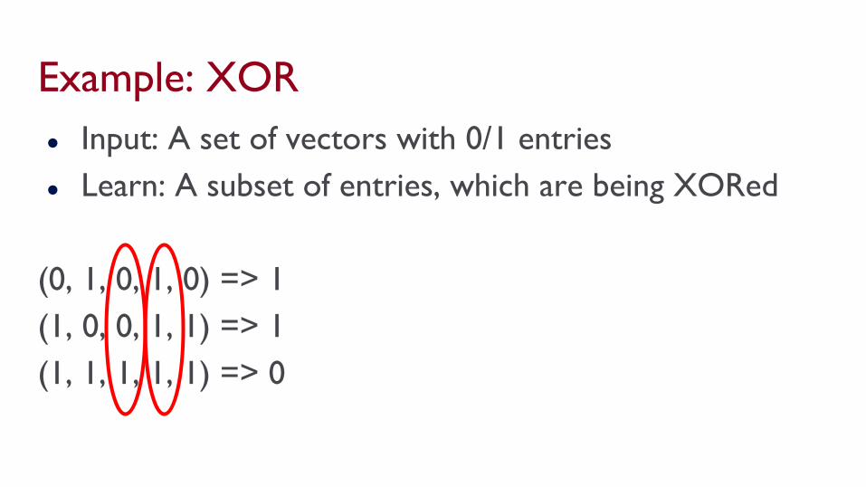
Example: XOR● Input: A set of vectors with 0/1 entries● Learn: A subset of entries, which are being XORed

(0, 1, 0, 1, 0) => 1(1, 0, 0, 1, 1) => 1(1, 1, 1, 1, 1) => 0

Example: XOR● Input: A set of vectors with 0/1 entries● Learn: A subset of entries, which are being XORed

(0, 1, 0, 1, 0) => 1(1, 0, 0, 1, 1) => 1(1, 1, 1, 1, 1) => 0

Example: XOR● Input: A set of vectors with 0/1 entries● Learn: A subset of entries, which are being XORed● Provably hard to work out by gradient descent● Entire loss landscape is flat except right around the

global minimum, which is very steep

How learning rate affects learning● If learning rate small, more likely to fall into a steep

minimum● Can be good if learning process is hard

Large learning rate a form of regularization● Fall into steep minima can be bad for generalization● The broader, flatter minima may be more robust● Larger learning rate => can be harder to learn, but

better generalization

Small batch size ⇔ large learning rate● Small batch size => noisy estimates of gradient● Also a way to improve generalization● Increasing the batch size is like decreasing the learning

rate● ½ learning rate can be interpreted as either 2 x batch

size or 4 x batch size, depending on perspective

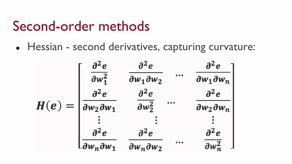
Second-order methods● Hessian - second derivatives, capturing curvature:

Why not always calculate the Hessian?

Why not always calculate the Hessian?● Number of entries is # params squared!● Too expensive generally● Some methods approximate the eigenvalues of the

Hessian

Cool picture: ResNet loss landscape

“Visualizing the loss landscapes of neural nets”, Li et al, NeurIPS 2018

Meta-learning

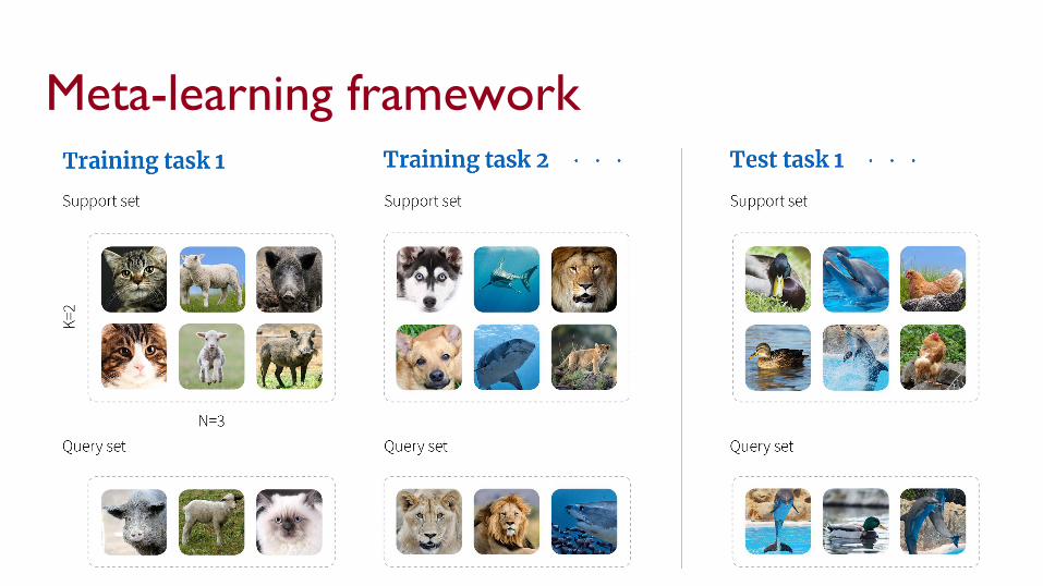
Meta-learning framework

Model-agnostic meta-learning (MAML)