Geomorphology 139–140 (2012) 495–505

Contents lists available at SciVerse ScienceDirect

Geomorphology

j ourna l homepage: www.e lsev ie r .com/ locate /geomorph

Cirque overdeepening and their relationship to morphometry

Marek Křížek ⁎, Klára Vočadlová, Zbyněk EngelDepartment of Physical Geography and Geoecology, Faculty of Science, Charles University in Prague, Albertov 6, 128 43 Praha 2, Czech Republic

⁎ Corresponding author. Tel.: +420 22 19 95 523; faE-mail addresses: krizekma@natur.cuni.cz (M. Křížek

(K. Vočadlová), engel@natur.cuni.cz (Z. Engel).

0169-555X/$ – see front matter © 2011 Elsevier B.V. Aldoi:10.1016/j.geomorph.2011.11.014

a b s t r a c t

a r t i c l e i n f o

Article history:Received 25 February 2011Received in revised form 18 November 2011Accepted 19 November 2011Available online 1 December 2011

Keywords:Cirque morphometryOverdeepeningk-curveBohemian Massif (the Czech Republic,Germany, Poland)

Shape and size characteristics of cirques and their changes and mutual relationships include not only spatialand descriptive aspects but also genetic attributes. The goals of this article were to define an application of k-curve (sensu Haynes, 1968) that describes the extent of cirque overdeepening and to identify k-curve equa-tion input variables. The k-values depend on the profile location, and hence, a clear definition of the cirqueprofile position is necessary. Therefore, ideal profiles were delineated through the steepest part of the cirqueheadwall (k-steepest, ks) or through a point on the cirque crest that had a maximal elevation (k-highest, kh).Knowledge of the cirque headwall height allows for the mathematical (theoretical) calculation of cirqueoverdeepening (i.e., the maximum depth of the cirque floor, sedimentary filling of the cirque floor). Further,the goal of this study was to analyse and compare cirque classification methods according to the extent ofoverdeepening and standard morphometric characteristics. As a training data set, 27 example cirques ofthe Bohemian Massif (Giant Mts., Šumava Mts., and Hrubý Jeseník Mts.) and a total of 12 morphometric char-acteristics were used in the analyses. Cirques were classified into two groups using cluster analysis based onthe extent of overdeepening (k-values: kh and ks). A mutual relationship between cluster analysis classifica-tions and classifications based on morphometric characteristics (L/W, H, and 3D/2D) was determined usinggeneral discriminant analysis. The classification of cirques based on other characteristics corresponded close-ly (in total, 81% for the first group and the cross-validation group) with cirque classifications based on the de-gree of overdeepening (k-value).

© 2011 Elsevier B.V. All rights reserved.

1. Introduction

In many published studies, cirques have been defined and charac-terised using a range of morphometric characteristics (Graf, 1976;Evans, 1977; Vilborg, 1977; Aniya and Welch, 1981; Evans and Cox,1995; Haynes, 1998; Davis, 1999; García-Ruiz et al., 2000; Federiciand Spagnolo, 2004; Brook et al., 2006; Ruiz-Fernández et al., 2009).In addition to the analysis of morphometric characteristics and evalua-tions of their mutual dependences, these studies also described the re-lationships between the size and shape characteristics of cirques andexposure, geological conditions, and the location of snow sources. Theaim of this article is not to study all relationships mentioned above,but to focus on determination of the degree of cirque overdeepeningusing k-curve (Haynes, 1968) and its comparison with cirque mor-phometry. From a mathematical point of view, this article analyses thequantities (variables) that enter into the k-curve and its subsequent ap-plication in real relief; although k-curve has been mentioned in somepublished studies, it has not been satisfactorily explained and its es-sence has not been described (Vilborg, 1977; Martini et al., 2001;Rasemann et al., 2004; Brook et al., 2006; Bennett and Glasser, 2009;Benn and Evans, 2010). A correct definition of k-curve as a part of glacial

x: +420 221 951 367.), vocadlov@natur.cuni.cz

l rights reserved.

erosion landform analyses can contribute to the identification of the de-velopment and intensity of mountain glaciation. Gordon (1977, p. 192)said that “if it is valid to assumea space–time transformation that cirquedevelopment is a function of cirque size, then the relationships betweenthe cirque size and shape variables have important implication for themode of cirque development.”

Another question is how cirque classification based on k-valuesdiffers from cirque classification based on commonly used morpho-metric characteristics. Cirques can be divided into categories accord-ing to their k-values and this classification can be combined withclassifications based on typical morphometric characteristics. Inother words, a chosen group of cirques can be categorised based onthe morphologic features (morphologic indices, sensu Evans andCox, 1995) and a genetic perspective (k-curve, sensu Haynes, 1968).

The main goals of this article are to define the use of k-curve as adescriptive index that characterises cirque overdeepening and to an-alyse and compare the classification of cirques according to the de-gree of overdeepening (k-curve) and standard morphometriccharacteristics based on cirques in the Bohemian Massif. The task ofthis paper is to determine whether the k-curve brings some new in-formation on the morphology of cirques, or whether it can beexpressed in other established morphometric characteristics.

Comparison of overdeepening (k-values) and morphometric char-acteristics was performed on 27 cirques in the Bohemian Massif.These cirques form a homogeneous group, with similar development

496 M. Křížek et al. / Geomorphology 139–140 (2012) 495–505

and shape of relief, the same character and age of glaciation, withsimilar paleoclimatic conditions and similar postglacial development.

2. Regional setting

During Pleistocene cold periods, the BohemianMassif was located ina periglacial zone in a foreland region of continental glaciation (Czudek,2005), andmountain glaciation occurred only in the northern (theHighSudetes) and southern (the ŠumavaMts.) fringes of the BohemianMas-sif. Small cirque glaciers, with tongues up to a few kilometres long, al-tered the relief and formed the cirques that are currently one of thedominant characteristic landforms of the local landscape. The relief ofglacial landforms in the Bohemian Massif was defined and describedas early as the nineteenth century (e.g., Bayberger, 1886; Partsch,1894). These reportswere followed by other studies on the glacialmod-ification of the High Sudetes (e.g., Vitásek, 1924; Prosová and Sekyra,1961; Chmal and Traczyk, 1999; Migoń, 1999; Mercier et al., 2000;Engel, 2007; Engel et al., 2010) and the Šumava Mts. (Rathsburg,1928; Priehäusser, 1930; Kunský, 1948; Ergenzinger, 1967; Votýpka,1979; Hauner, 1980; Raab and Völkel, 2003; Vočadlová et al., 2007;Vočadlová and Křížek, 2009; Mentlík et al., 2010); however complexcomparative studies have not been carried out.

The Bohemian Massif is a Hercynian geological unit (Chlupáč et al.,2002) and includes the majority of the Czech Republic and parts ofthe frontier regions of Germany, Poland, and Austria (Fig. 1). TheHigh Sudetes and the Šumava Mts. are fault-block ranges with

Fig. 1. Distribution of cirques

summit plateaus and this terrain had an important role in the originof the Late Pleistocene mountain glaciation. Snow that was blownfrom summit plateaus by prevailing westerly winds (Meyer andKottmeier, 1989; Isarin et al., 1997) onto leeward preglacial valleyheads helped to create cirque and valley glaciers with tongues thatare only a few hundred metres to a few kilometres long (Jeník,1961). Deglaciation of the Bohemian Massif occurred at the end ofthe Late Pleistocene.

The Šumava Mts. (called the Bavarian Forest on the German sideand the Bohemian Forest on the Czech side of the state border,Fig. 1) are mainly composed of metamorphic rocks (gneisses, micaschists, phyllites, granulites, and migmatites) permeated by youngerigneous rocks (granites, tonalities, and granodiorites) (Babůrek etal., 2006). The highest peak is Grosser Arber (1456 m asl). In themountain range, eight of 13 cirques are filled with lakes: Černé jezero,Čertovo jezero, Laka, Prášilské jezero (compound cirque), Plešnéjezero, Kleiner Arbersee, Grosser Arbersee, and Rachelsee. The pre-dominant view is that a smaller extent of glacier covers (cirque orshort valley glaciers) was present here in times of maximal glaciation(Hauner, 1980; Raab, 1999; Reuther, 2007). Evidence of the LatePleistocene glaciation (MIS 2) in the Šumava Mts. has been found, al-though no convincing evidence for older glaciation has been existed(Bayberger, 1886; Rathsburg, 1928; Priehäusser, 1930; Ergenzinger,1967; Hauner, 1980). The Pleistocene snow equilibrium line altitude(according to the maximum elevation of lateral moraines method,MELM) corresponding to the last glaciation was found between 925

in the Bohemian Massif.

497M. Křížek et al. / Geomorphology 139–140 (2012) 495–505

and 1115 m asl (Hauner, 1980; Raab, 1999; Vočadlová and Křížek,2005; Mentlík et al., 2010). Recent research in the Šumava Mts. hasshown that the cirque floors were free of ice prior to ~14,500–14,000 cal YBP (Raab and Völkel, 2003; Reuther, 2007; Mentlík etal., 2010)

The Giant Mts. (called Krkonoše on the Czech side and Karkonoszeon the Polish side of the state borders) represent the western part ofthe High Sudetes and mainly consist of Proterozoic and Paleozoicmethamorphites (gneiss, mica schist, phyllite, and quartzite) and plu-tonic rocks (granite) can be found (Chlupáč et al., 2002). This moun-tain range on the Czech and Polish border has fault-generatedmountain fronts on the southern and northern side, extended summitplateaus (area up to a few square kilometres). Mt. Sněžka (1602 masl) is the highest peak. The front of the Scandinavian ice sheetapproached immediately the northern foreground of the Giant Mts.during the Early Saalian (MIS8, 440–430 ka BP) (Hall and Migoń,2010). More morphologic evidence of glacial alteration has beenobtained from the Giant Mts. than from all other studied ranges of

Fig. 2. Cirques of the Šumava Mt

the Bohemian Massif. A total of 13 cirques (six on the Polish side,seven on the Czech side) have been described in this region. Tonguesof the largest glaciers on the Czech side of the Giant Mts. (glacier ofLabský důl valley and Obří důl valley) reached a maximum of up to5 km in length (Králík and Sekyra, 1969). An equilibrium snow line al-titude occurred at 1060–1170 masl during the oldest glacier oscillation atthe end of the Pleistocene. Glacial accumulation landforms from the lastWürm glaciation were preserved on the Czech side, whereas relicts alsoof Riss moraines were found on the Polish side (Traczyk, 1989; Chmaland Traczyk, 1999). Recent research has shown that the last phase of de-glaciation occurred prior to ~11,000 cal YBP (Engel et al., 2010).

The Hrubý Jeseník Mts. form the eastern part of the High Sudetesand are mainly composed of metamorphic rocks (gneiss, mica schist,phyllite, quartzite, and erlan) (Chlupáč et al., 2002). The main ridge ofthe Hrubý Jeseník Mts. that includes summit plateaus (1300–1450 masl) has a north–south orientation. Mount Praděd (1492 m asl) is thehighest peak. Today, this mountain range has the lowest rate of glacialmodification because of constrains imposed by preglacial relief

s. with marked median axis.

498 M. Křížek et al. / Geomorphology 139–140 (2012) 495–505

(Migoń, 1999) and the low resistance of rocks which contributed torapid weathering and big rate of postglacial modification of the relief.Only one cirque, Velká kotlina, can be found in the valley head of theMoravice River (Prosová, 1958; Czudek, 2005). This cirque has aneast–southeast position relative to the main ridge of the Hrubý Jese-ník Mts. and is situated below its largest summit plateau, which sup-plied the glacier with snow. This glacier was 600 m in length(Prosová, 1958), and its terminal moraine is situated at 1060 m aslThe snowline altitude of the glacier during the last glaciation was de-fined by Vitásek (1924) to be 1150 m asl, which approximately corre-sponds with the altitude of the cirque floor.

3. Methodological approach

3.1. Morphometric (planimetric and hypsometric) characteristics of cirques

Calculations associated with the determination of planimetric andhypsometric indices that describe cirques were used for morphomet-ric analyses. The most frequently used indices that define the size and

Fig. 3. Cirques of the High Sudete

shape of cirques were chosen. Data used for morphometric analyseswere acquired from published geomorphologic studies, from aerialphotos, from a digital elevation model (DEM), and from field map-ping. A DEM of 3×3 m pixel size was created from the contour dataof military topographic maps DMÚ 25 at a scale of 1:25,000 with a5-m contour interval and a basic positional accuracy of up to 10 m.Cirque borders were delineated according to the crest limit andthreshold and by the moraine crest line if the moraine covered thethreshold. Step-like cirques were considered as one unit where thelowest-lying cirque was included to analyse landforms correspondingtomaximal extent of glaciation in a particular locality (Kleiner Arbersee,Grosser Arbersee, Grosser Rachel-Altersee, and Prášilské jezero). A totalof 27 cirques were analysed (five cirques on the Czech side of theŠumava Mts., eight cirques on the German side of the Šumava Mts.,seven cirques on the Czech side of the GiantMts., six cirques on the Pol-ish side of the Giant Mts., and one cirque in the Hrubý Jeseník Mts.)(Figs. 2 and 3).

The following features that describe the cirque size were used inthe morphometric analysis: height (H), length (L), width (W), plan

s with marked median axis.

499M. Křížek et al. / Geomorphology 139–140 (2012) 495–505

area (2D, area of the planar projection of the relief), volume (V), meanslope, aspect of the cirque median axis, and surface area (3D, area ofthe real relief). Based on these measurements, indices that describethe shape of cirques were calculated: cirque length to height ratio(L/H), cirque length to width ratio (L/W), width to height ratio (W/H),and the surface area to plan area ratio (3D/2D).

The cirque height (H) represented the difference between thelowest and the highest altitude within a cirque (sensu Aniya andWelch, 1981; García-Ruiz et al., 2000; Federici and Spagnolo, 2004).Similar to other studies (Evans and Cox, 1995; Federici andSpagnolo, 2004), cirque length (L) was measured along the medianaxis — a line drawn from the cirque focus (middle of cirque thresh-old) to the crest — such that the area on the left was equal to thearea on the right. The (maximum) width (W) was measured at aright angle to the median axis. Altitudes (Emin., Emax., and Emean), cir-que areas (2D and 3D), and the mean gradient were derived fromthe DEM by using GIS tools. Cirque volume (V) was calculated asV=0.5(H×L×W) (Gordon, 1977; Davis, 1999). The cirque aspectswere defined as the median axis aspect and were classified intoeight categories: N, NE, E, SE, S, SW, W, and NW. The DEM was usedto derive the cirque plan areas (2D) based on the area of the ortho-graphic floor projection of the cirque. The cirque surface areas (3D)were derived from the DEM and represented the actual area of a cir-que surface. The 3D/2D ratio reflected an area-relative elevation rela-tionship (vertical relief segmentation; relative relief) of a cirque. TheL/H ratio (gradient) illustrated the cross-sectional shape of the cirque,L/W ratio described the planimetric shape (indicated circularity orcirque elongation), and the W/H ratio indicated the extent of cirqueincision (Graf, 1976; García-Ruiz et al., 2000).

3.2. Construction, characteristics and application of k-curve

Cirque overdeepening is defined by a k-coefficient based on theequation

y ¼ k 1−xð Þe−x ð1Þ

which is called the k-curve (Haynes, 1968) (Fig. 4). To calculate ak-curve, a longitudinal section of a cirque was constructed, and thehorizontal (a) and vertical (β) distances between the headwall crestand headwall foot were determined. These data were used for the cal-culation of k-coefficients. Headwall foot positions were determinedbased on the shape of the longitudinal section curve. Twok-coefficients were calculated for each cirque depending on the loca-tion of the longitudinal profile. The first k-coefficient (k-steepest, ks)was calculated based on the profile crossing the steepest part of thecirque headwall, and the second k-coefficient (k-highest, kh) was cal-culated based on the profile running down from a point on the cirque

Fig. 4. Graph of the k-curve for k=2. Input variables that are used for the calculation ofk-curves are marked. E — cirque crest, F — headwall foot, and D — deepest point of thecirque floor.

crest with a maximal altitude across the cirque floor. Lines of bothprofiles went perpendicularly through the contours and passed asclosely as possible through the lowest part of the cirque floor.

The domain of definition of Eq. (1) was (−∞,+∞); however, withrespect to x, which described the lengths, we accepted that the do-main of this function was (0,+∞). Other characteristics of the k-curve resulted from the first (Eq. (2)) and second derivatives(Eq. (3)) of the k-curve function (Eq. (1)); i.e.

y′ ¼ −ke−x 2−xð Þ ð2Þ

y″ ¼ ke−x 3−xð Þ: ð3Þ

For the first derivative, y′=0 when x=2; the second derivative atpoint x=2 was nonzero. Therefore, it followed that the functionEq. (1) had a local extreme at point x=2. The first derivativeEq. (2) showed that y′b0 within the interval (0,2) and y′>0 in the in-terval (2,∞). The k-curve function (Eq. (1)) reached a local minimumat the point x=2. Therefore, the k-curve ran through the deepestpoint of the cirque. Thus, the k-value could be defined based on thedifference in altitude between the lowest point of the cirque andthe foot of cirque headwall (Fig. 4) because values X0 (horizontal dis-tance between the deepest point of the cirque and the cirque crest)and Y0 (difference in elevation between the deepest point of the cir-que and the foot of the cirque headwall) could be determined by geo-morphologic mapping. However, it is necessary to transform the realvalues X0 and Y0 (presented in metres or kilometres) into k-curvemetrics and make computations using these transformed values. Inother words, for the deepest point of the cirque (x=2), k=−ye2

where the y value was defined as y=2Y0/X0, whereas the value Y0had a negative sign with respect to the defined coordinate system(see Fig. 4).

Another important characteristics resulting from the k-curve function(Eq. (1))was the relationship between the cirquefloor deepening (α; cir-quefloor deepeningmeans an elevation difference between the headwallfoot and the cirque floor) and the height of the cirque headwall (β; cirqueheadwall height means an elevation difference between the headwallfoot and the headwall crest) that was constant and corresponded to α/β=−e−2. When calculating β, x=0 for the cirque crest, and conse-quently, y=k(1–0)e−0 and y=k; when calculating α with x=2,y=k(1–2)e−2, and y=−ke−2. A constantα/β ratiowas used as amath-ematical approximation of the cirque floor deepening based on knowl-edge of the cirque headwall height, which was multiplied by −e−2.This procedure was used in cases where the cirque floor was coveredby sediments of unknown thickness or by a lake of unknown depth.

Based on the definition and character of the k-curves, evident is thatk-coefficient could never be negative because β=k and α=−ke−2.Otherwise, the basic presumption that a cirque crest was situatedhigher than the foot of the cirque headwall of the appropriate cirquewould not be valid.

3.3. Statistical evaluation

All statistical operations were performed using the programmeSTATISTICA (StatSoft, Inc., 2009). The studied cirques were dividedinto groups based on cluster analysis (tree clustering), with the ap-propriate values of kh and ks as the input variables of correlation mor-phometric characteristics were expressed as Pearson correlationcoefficients, with the significance of differences in single characteris-tics was tested using t-tests with a confidence level of p=0.05.

General discriminant analysis (GDA) was executed for a selectsubset of all studied morphometric characteristics (basis). The basisof the morphometric characteristics was explicitly defined as the larg-est set of independent morphometric characteristics (i.e., those char-acteristics that were not mutually correlated). The choice of basis

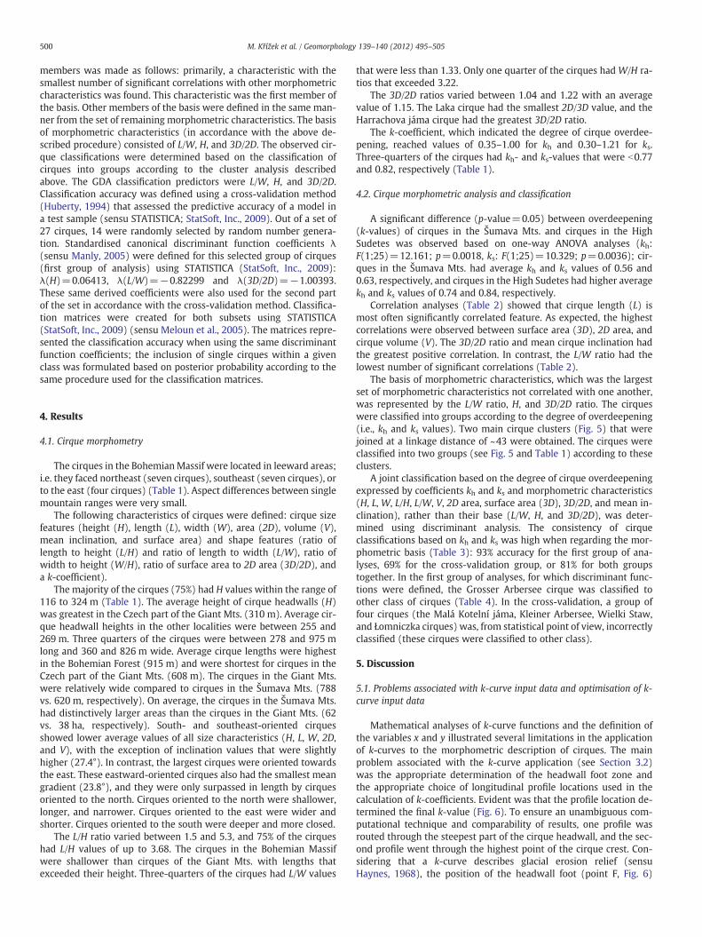
500 M. Křížek et al. / Geomorphology 139–140 (2012) 495–505

members was made as follows: primarily, a characteristic with thesmallest number of significant correlations with other morphometriccharacteristics was found. This characteristic was the first member ofthe basis. Other members of the basis were defined in the same man-ner from the set of remaining morphometric characteristics. The basisof morphometric characteristics (in accordance with the above de-scribed procedure) consisted of L/W, H, and 3D/2D. The observed cir-que classifications were determined based on the classification ofcirques into groups according to the cluster analysis describedabove. The GDA classification predictors were L/W, H, and 3D/2D.Classification accuracy was defined using a cross-validation method(Huberty, 1994) that assessed the predictive accuracy of a model ina test sample (sensu STATISTICA; StatSoft, Inc., 2009). Out of a set of27 cirques, 14 were randomly selected by random number genera-tion. Standardised canonical discriminant function coefficients λ(sensu Manly, 2005) were defined for this selected group of cirques(first group of analysis) using STATISTICA (StatSoft, Inc., 2009):λ(H)=0.06413, λ(L/W)=−0.82299 and λ(3D/2D)=−1.00393.These same derived coefficients were also used for the second partof the set in accordance with the cross-validation method. Classifica-tion matrices were created for both subsets using STATISTICA(StatSoft, Inc., 2009) (sensu Meloun et al., 2005). The matrices repre-sented the classification accuracy when using the same discriminantfunction coefficients; the inclusion of single cirques within a givenclass was formulated based on posterior probability according to thesame procedure used for the classification matrices.

4. Results

4.1. Cirque morphometry

The cirques in the BohemianMassif were located in leeward areas;i.e. they faced northeast (seven cirques), southeast (seven cirques), orto the east (four cirques) (Table 1). Aspect differences between singlemountain ranges were very small.

The following characteristics of cirques were defined: cirque sizefeatures (height (H), length (L), width (W), area (2D), volume (V),mean inclination, and surface area) and shape features (ratio oflength to height (L/H) and ratio of length to width (L/W), ratio ofwidth to height (W/H), ratio of surface area to 2D area (3D/2D), anda k-coefficient).

The majority of the cirques (75%) had H values within the range of116 to 324 m (Table 1). The average height of cirque headwalls (H)was greatest in the Czech part of the Giant Mts. (310 m). Average cir-que headwall heights in the other localities were between 255 and269 m. Three quarters of the cirques were between 278 and 975 mlong and 360 and 826 m wide. Average cirque lengths were highestin the Bohemian Forest (915 m) and were shortest for cirques in theCzech part of the Giant Mts. (608 m). The cirques in the Giant Mts.were relatively wide compared to cirques in the Šumava Mts. (788vs. 620 m, respectively). On average, the cirques in the Šumava Mts.had distinctively larger areas than the cirques in the Giant Mts. (62vs. 38 ha, respectively). South- and southeast-oriented cirquesshowed lower average values of all size characteristics (H, L, W, 2D,and V), with the exception of inclination values that were slightlyhigher (27.4°). In contrast, the largest cirques were oriented towardsthe east. These eastward-oriented cirques also had the smallest meangradient (23.8°), and they were only surpassed in length by cirquesoriented to the north. Cirques oriented to the north were shallower,longer, and narrower. Cirques oriented to the east were wider andshorter. Cirques oriented to the south were deeper and more closed.

The L/H ratio varied between 1.5 and 5.3, and 75% of the cirqueshad L/H values of up to 3.68. The cirques in the Bohemian Massifwere shallower than cirques of the Giant Mts. with lengths thatexceeded their height. Three-quarters of the cirques had L/W values

that were less than 1.33. Only one quarter of the cirques had W/H ra-tios that exceeded 3.22.

The 3D/2D ratios varied between 1.04 and 1.22 with an averagevalue of 1.15. The Laka cirque had the smallest 2D/3D value, and theHarrachova jáma cirque had the greatest 3D/2D ratio.

The k-coefficient, which indicated the degree of cirque overdee-pening, reached values of 0.35–1.00 for kh and 0.30–1.21 for ks.Three-quarters of the cirques had kh- and ks-values that were b0.77and 0.82, respectively (Table 1).

4.2. Cirque morphometric analysis and classification

A significant difference (p-value=0.05) between overdeepening(k-values) of cirques in the Šumava Mts. and cirques in the HighSudetes was observed based on one-way ANOVA analyses (kh:F(1;25)=12.161; p=0.0018, ks: F(1;25)=10.329; p=0.0036); cir-ques in the Šumava Mts. had average kh and ks values of 0.56 and0.63, respectively, and cirques in the High Sudetes had higher averagekh and ks values of 0.74 and 0.84, respectively.

Correlation analyses (Table 2) showed that cirque length (L) ismost often significantly correlated feature. As expected, the highestcorrelations were observed between surface area (3D), 2D area, andcirque volume (V). The 3D/2D ratio and mean cirque inclination hadthe greatest positive correlation. In contrast, the L/W ratio had thelowest number of significant correlations (Table 2).

The basis of morphometric characteristics, which was the largestset of morphometric characteristics not correlated with one another,was represented by the L/W ratio, H, and 3D/2D ratio. The cirqueswere classified into groups according to the degree of overdeepening(i.e., kh and ks values). Two main cirque clusters (Fig. 5) that werejoined at a linkage distance of ~43 were obtained. The cirques wereclassified into two groups (see Fig. 5 and Table 1) according to theseclusters.

A joint classification based on the degree of cirque overdeepeningexpressed by coefficients kh and ks and morphometric characteristics(H, L, W, L/H, L/W, V, 2D area, surface area (3D), 3D/2D, and mean in-clination), rather than their base (L/W, H, and 3D/2D), was deter-mined using discriminant analysis. The consistency of cirqueclassifications based on kh and ks was high when regarding the mor-phometric basis (Table 3): 93% accuracy for the first group of ana-lyses, 69% for the cross-validation group, or 81% for both groupstogether. In the first group of analyses, for which discriminant func-tions were defined, the Grosser Arbersee cirque was classified toother class of cirques (Table 4). In the cross-validation, a group offour cirques (the Malá Kotelní jáma, Kleiner Arbersee, Wielki Staw,and Łomniczka cirques) was, from statistical point of view, incorrectlyclassified (these cirques were classified to other class).

5. Discussion

5.1. Problems associated with k-curve input data and optimisation of k-curve input data

Mathematical analyses of k-curve functions and the definition ofthe variables x and y illustrated several limitations in the applicationof k-curves to the morphometric description of cirques. The mainproblem associated with the k-curve application (see Section 3.2)was the appropriate determination of the headwall foot zone andthe appropriate choice of longitudinal profile locations used in thecalculation of k-coefficients. Evident was that the profile location de-termined the final k-value (Fig. 6). To ensure an unambiguous com-putational technique and comparability of results, one profile wasrouted through the steepest part of the cirque headwall, and the sec-ond profile went through the highest point of the cirque crest. Con-sidering that a k-curve describes glacial erosion relief (sensuHaynes, 1968), the position of the headwall foot (point F, Fig. 6)

Table 1Morphometric characteristics of the Bohemian Massif cirques.

Cirque name GPS position kh ks Emax. Emin. Emean H(m)

L(m)

W(m)

L/H L/W W/H

Volume(106 m3)

2Darea(ha)

Surfacearea(ha)

3D/2D

Meangradient(°)

Medianaxisaspect

Lithologya

Černé jezero 49° 10′ 46″ N,13° 10′ 57″ E

0.74 0.76 1321 968 1084 353 1111 887 3.15 1.25 2.52 173.74 86.32 100.09 1.16 25 NE MS

Čertovo jezero 49° 09′ 54″ N,13° 11′ 48″ E

0.54 0.60 1315 992 1116 323 901 1100 2.79 0.82 3.40 160.21 71.42 78.57 1.10 23 E MS, PG

Laka 49° 06′ 37″ N,13° 19′ 40″ E

0.39 0.39 1304 1081 1157 223 1080 803 4.84 1.34 3.60 96.70 68.92 71.93 1.04 15 NE PG, GD

Prášilskéjezerob

49° 04′ 31″ N,13° 23′ 59″ E

0.55 0.58 1210 1062 1156 148 476 386 3.22 1.23 2.61 11.02 14.09 15.26 1.08 20 E G, PG

Plešné jezero 48° 46′ 35″ N,13° 51′ 54″ E

0.70 0.70 1342 1068 1174 274 1008 760 3.68 1.33 2.77 104.95 53.66 60.90 1.13 25 NE G, PG

GrosserArbersee

49° 05′ 54″ N,13° 09′ 03″ E

0.89 0.79 1292 918 1062 374 1212 1467 3.24 0.83 3.92 332.49 154.53 171.49 1.11 22 E GN

Rachelsee 48° 58′ 38″ N,13° 24′ 04″ E

0.56 0.72 1263 1057 1150 206 809 608 3.93 1.33 2.95 50.66 37.26 41.41 1.11 23 S GN

GrosserRachel-AlterSee

48° 58′ 28″ N,13° 23′ 36″ E

0.62 0.58 1437 1077 1213 360 820 830 2.28 0.99 2.31 122.51 56.60 63.83 1.13 26 SE GN

Kleiner Rachel 48° 59′ 19″ N,13° 23′ 09″ E

0.51 0.64 1281 1070 1155 211 982 761 4.65 1.29 3.61 78.84 53.21 58.14 1.09 21 N GN

KleinerArbersee

49° 07′ 28″ N,13° 07′ 10″ E

0.35 0.41 1268 907 1059 361 1798 1090 4.98 1.65 3.02 353.75 148.09 162.99 1.10 22 N GN

Hirschbach 49° 02′ 32″ N,13° 22′ 23″ E

0.44 0.64 1237 1085 1165 152 407 382 2.68 1.07 2.51 11.82 11.01 12.24 1.11 25 S MS

Hirschbach IIc 49° 01′ 47″ N,13° 21′ 48″ E

0.42 0.30 1061 945 999 116 453 447 3.91 1.01 3.85 11.74 16.18 17.34 1.07 19 SE GR

Schwarzbachd 48° 57′ 17″ N,13° 32′ 08″ E

0.56 0.72 1272 1016 1107 256 675 718 2.64 0.94 2.80 62.04 36.83 41.36 1.12 23 SE GR

Malá Kotelníjáma

50° 44′ 52″ N,15° 32′ 03″ E

0.61 0.64 1421 1097 1246 324 590 360 1.82 1.64 1.11 34.41 18.13 21.99 1.21 32 SE PH, GN

Velká Kotelníjáma

50° 45′ 02″ N,15° 32′ 14″ E

0.79 0.74 1406 1125 1275 281 502 640 1.79 0.78 2.28 45.14 25.39 30.64 1.21 32 S PH, MS,GR

Labský důl 50° 46′ 07″ N,15° 33′ 07″ E

0.80 0.77 1303 1018 1124 285 975 770 3.42 1.27 2.70 106.98 62.18 74.23 1.19 27 SE GR

Harrachovajáma

50° 45′ 18″ N,15° 33′ 10″ E

1.00 I.21 1353 1168 1270 185 278 555 1.50 0.50 3.00 14.27 11.84 14.42 1.22 34 NE GR

Úpská jáma 50° 43′ 59″ N,15° 43′ 22″ E

0.61 0.74 1498 1045 1250 453 782 1300 1.73 0.60 2.87 230.26 86.29 101.96 1.18 30 E GR, GD

VelkáStudničníjáma

50° 43′ 17″ N,15° 42′ 46″ E

0.79 0.79 1500 1114 1266 386 724 367 1.88 1.97 0.95 51.28 21.62 25.63 1.19 30 S PH, MS

MaláStudničníjáma

50° 43′ 30″ N,15° 43′ 01″ E

0.74 0.78 1478 1222 1334 256 405 380 1.58 1.07 1.48 19.70 12.34 14.78 1.20 32 SE PH, MS

Mały ŚnieżnyKocioł

50° 46′ 56″ N,15° 33′ 25″ E

0.64 I.15 1476 1181 1306 295 726 440 2.46 1.65 1.49 47.12 25.77 31.04 1.20 30 NE GR

WielkiŚnieżnyKocioł

50° 46′ 47″ N,15° 33′ 39″ E

0.83 0.85 1488 1246 1330 242 805 526 3.33 1.53 2.17 51.24 34.88 41.99 1.20 29 N GR

Czarny Kocioł 50° 46′ 58″ N,15° 35′ 08″ E

0.73 0.85 1346 1117 1202 229 473 413 2.07 1.15 1.80 22.37 14.91 17.73 1.19 30 N GR

Wielki Staw 50° 45′ 31″ N,15° 41′ 33″ E

0.72 0.82 1403 1200 1276 203 581 757 2.86 0.77 3.73 44.64 36.88 41.94 1.14 23 NE GR

Mały Staw 50° 44′ 52″ N,15° 42′ 05″ E

0.70 0.84 1391 1108 1225 283 1507 934 5.33 1.61 3.30 199.17 101.84 114.62 1.13 23 N GR

Łomniczka 50° 44′ 30″ N,15° 44′ 02″ E

0.56 0.74 1411 1051 1222 360 899 826 2.50 1.09 2.29 133.66 63.44 74.66 1.18 30 NE GR

Velká kotlina 50° 03′ 18″ N,17° 14′ 19″ E

0.82 0.83 1350 1156 1258 194 299 405 1.54 0.74 2.09 11.75 9.79 11.86 1.21 33 SE PH

Emax., min., mean — maximal, minimal and mean cirque elevation in m asl.a Lithology: MS — mica schist, PG — paragneis, GD — granodiorite, GR — granite, GN — gneiss, and PH — phyllite.b In the work of Mentlík et al. (2010), this feature is described as “lower cirque.”c In the work of Ergenzinger (1967), this feature is described as Wiesriegelkar.d In the work of Ergenzinger (1967), this feature is described as Bärenriegelkar.

501M. Křížek et al. / Geomorphology 139–140 (2012) 495–505

within the profile should have ignored the regions of a cirque thatwere post-glacially altered and minimised the likelihood that nongla-cial landforms were described instead of glacial features. Therefore, itis necessary to abstract glacial and postglacial accumulation land-forms (e.g., moraines, slope talus, and debris-flows) that could haveinfluenced the shape of the longitudinal profile curve and, conse-quently, the placement of the headwall foot. This correction could

be carried out using an extrapolation of the bedrock line in the footof the cirque headwall and possibly the cirque bottom.

5.2. Informative value of k-curve

In addition to k-coefficients, the rate of cirque overdeepening canalso be characterised by several morphometric traits. Correlation

Table 2Correlation matrices of morphometric characteristics of the studied cirques; marked correlations (bold) were significant at pb0.05 as determined using t-tests (N=27).

Variable H L W L/H L/W W/H V 2D area 3D area 3D/2D Mean gradient

H 1.00 0.51 0.61 −0.20 0.15 −0.28 0.69 0.60 0.62 0.27 0.27L 0.51 1.00 0.69 0.70 0.44 0.33 0.85 0.89 0.89 −0.39 −0.46W 0.61 0.69 1.00 0.30 −0.27 0.57 0.90 0.90 0.91 −0.32 −0.33L/H −0.20 0.70 0.30 1.00 0.42 0.63 0.38 0.50 0.48 −0.74 −0.82L/W 0.15 0.44 −0.27 0.42 1.00 −0.40 0.05 0.07 0.07 −0.04 −0.14W/H −0.28 0.33 0.57 0.63 −0.40 1.00 0.36 0.46 0.44 −0.74 −0.75V 0.69 0.85 0.90 0.38 0.05 0.36 1.00 0.98 0.98 −0.27 −0.282D area 0.60 0.89 0.90 0.50 0.07 0.46 0.98 1.00 1.00 −0.36 −0.403D area 0.62 0.89 0.91 0.48 0.07 0.44 0.98 1.00 1.00 −0.32 −0.373D/2D 0.27 −0.39 −0.32 −0.74 −0.04 −0.74 −0.27 −0.36 −0.32 1.00 0.96Mean gradient 0.27 −0.46 −0.33 −0.82 −0.14 −0.75 −0.28 −0.40 −0.37 0.96 1.00

502 M. Křížek et al. / Geomorphology 139–140 (2012) 495–505

analyses (Table 3) of the studied group of cirques showed thatk-values correlated with L/H, 3D/2D ratios, and mean cirque gradi-ents; whereas the highest correlation coefficient value (0.73) was ob-served for the 3D/2D ratio. The best means of approximating k-valuesusing classic morphometric tools is the expression using surface area,cirque planform ratio (3D/2D) or mean gradient.

Based on theories of cirque development over time (Gordon,1977; Olyphant, 1981; Brook et al., 2006; Evans, 2006), we can as-sume that k-values change as a cirque ages. Based on the develop-ment of diagrams of long profile time evolution according toGordon (1977) and later in similar works (Brook et al., 2006; Evans,2006), k-values can be determined using a simple calculation; thesediagrams also illustrate that the change in k-values over time is linearfor cirques in alpine and highland relief environments. Thek-coefficients appear to be a strong expression of the degree of cirquedevelopment.

Differences in both morphometric characteristics (see above) andk-values for cirques in the Šumava Mts. and the High Sudetes werealso observed. The cirques in the High Sudetes had a greater degreeof overdeepening than cirques in the Šumava Mts. A greater extentof overdeepening of cirques in the High Sudetes probably relates toa more extensive and intense glaciation. Deglaciation of the Šumava

Fig. 5. Tree clustering of cirques according to k-highest and k-steepest (Euc

Mts. (Raab, 1999; Mentlík et al., 2010) occurred much earlier thanin the Giant Mts. (Engel et al., 2010).

This difference cannot be explained by differences in lithology be-cause one-way ANOVA did not show (95% significance level) a signif-icant relationship between lithologic type and kh and ks values.

5.3. Cirque classifications

Previously published cirque classifications have been either onlydescriptive, by taking into account cirque genesis together with to-pography or geology (Rudberg, 1954; Trenhaile, 1976; Gordon,1977; Vilborg, 1977); or as in the case of recent classifications, theyhave taken into account basic morphometric size and shape charac-teristics together with the cirque geology or aspect (García-Ruiz etal., 2000; Ruiz-Fernández et al., 2009). García-Ruiz et al. (2000) clas-sified 194 cirques of the central Pyrenees (Spain) into four groupsusing cluster analysis (minimization of Euclidean distances and selec-tion from the dendrogram) based on certain morphometric charac-teristics (L, W, H, A, L/W, and L/H). These authors noted that theiranalyses showed that certain environmental variables (altitude, as-pect, and lithology) had a limited influence on both the shape andsize variables of those glacial cirques. Discriminant analysis showed

lidean distance measures and amalgamation rule by Ward's method).

Table 3Classification matrix for the first group of analyses: randomly chosen cirque for whichthe discriminant function coefficients were defined, the second cross-validation groupand both groups together.

Class 1st group analysis (%) Cross-validation (%) Both (%)

X 88.89 83.33 86.67Y 100.00 57.14 75.00Total 92.86 69.23 81.48

503M. Křížek et al. / Geomorphology 139–140 (2012) 495–505

that altitude, aspect, and lithology explained the classification of only~66% of the Pyrenean cirques. The other discriminating factors wereascribed to the influence of the presence of faults, the resistance ofrocks and preglacial relief. Studies of cirque morphometry from dif-ferent parts of the world (Aniya and Welch, 1981; Evans and Cox,1995; García-Ruiz et al., 2000; Federici and Spagnolo, 2004; Hugheset al., 2007; Ruiz-Fernández et al., 2009) have shown that the influ-ence of all the above-mentioned factors on the size and shape of cir-ques cannot be generalised.

According to the successful classification performed using GDA(Table 3), the existence of a close relationship between the degreeof overdeepening and morphometric characteristics was detectedfor the group of Bohemian Massif cirques studied here. Cirque classi-fications based on k-values coincided with morphometric-based clas-sifications in 81% of the cases. In other words, the classification ofcirques based on a genetic perspective (k-curve as defined byHaynes, 1968) is compatible with classification methods based on cir-que morphology (morphological indices in accordance with Evansand Cox, 1995). Therefore, this study demonstrated that the classifi-cation of cirques according to the degree of overdeepening corre-sponded more closely with cirque morphometry than withenvironmental variables, as shown by García-Ruiz et al. (2000) andRuiz-Fernández et al. (2009).

Table 4Posterior probabilities of classifications; incorrect classifications are marked with *;cirques from the first group of analyses (which defined the discriminant function coef-ficients) are marked with a bold italic font; observed classifications were based on khand ks in two classes X and Y.

Cirque name Observed class X Y

Černé jezero X 0.88 0.12Čertovo jezero Y 0.10 0.90Laka Y 0.14 0.86Prášilské jezero Y 0.32 0.68Plešné jezero X 0.81 0.19Velká kotlina X 0.85 0.15Malá Kotelní jáma* Y 1.00 0.00Velká Kotelní jáma X 0.84 0.16Labský důl X 0.97 0.03Harrachova jáma X 0.71 0.29Úpská jáma* Y 0.42 0.58Velká Studniční jáma X 1.00 0.00Malá Studniční jáma X 0.93 0.07Grosser Arbersee* X 0.13 0.87Rachelsee X 0.66 0.34Grosser Rachel-Alter See Y 0.38 0.62Kleiner Rachel Y 0.44 0.56Kleiner Arbersee* Y 0.82 0.18Hirschbach Y 0.39 0.61Hirschbach II Y 0.10 0.90Schwarzbach Y 0.32 0.68Mały Śnieżny Kocioł X 1.00 0.00Wielki Śnieżny Kocioł X 0.99 0.01Czarny Kocioł X 0.94 0.06Wielki Staw* X 0.28 0.72Mały Staw X 0.92 0.08Łomniczka* Y 0.86 0.14

Divergences in cirque classifications, or incorrect categorizationinto groups, can be explained in several ways: (i) Although itemerged that k-curves are related (a significant correlation existed)to some morphometric characteristics [kh vs. L/H (−0.50), 3D/2D(0.70), mean gradient (0.62); ks vs. L/H (−0.42), 3D/2D (0.65),mean gradient (0.61)], k-curves provide different information andcannot be replaced entirely by morphometric methods. In otherwords, a difference exists between strictly morphological characteris-tics (sensu Evans and Cox, 1995) and genetic aspects of cirques thatare represented by k-curves (sensu Haynes, 1968). (ii) The set ofstandard morphometric characteristics does not have to be complete,or other independent sizes or indices that could better characterise acirque from a genetic perspective can be missing. (iii) If the set ofstudied cirques with an analogous genesis was larger, the influenceof abnormally-developed cirques would be statistically low. A betterdetermination of cirque groups could be obtained by addressingthese factors.

6. Conclusions

Mathematical analyses were used to demonstrate the potentialbenefits and limitations of using k-curves in real scenarios:

(i) It is necessary to correctly and unequivocally identify the lon-gitudinal profile and input variables (position of the crest andcirque headwall or the deepest point of the cirque) to obtaina correct definition of the k-value. The k-values cannot be neg-ative. The ratio between the height of the headwall and cirquefloor deepening is constant and does not depend on the valueof the k-coefficient.

(ii) Knowledge of the cirque headwall height allows for the math-ematical calculation (theoretical) of cirque overdeepening(i.e., the maximum depth of the cirque floor). If the k-curvecould be considered as approximation to the longitudinalprofile of cirque, then it is possible according to the k-curveequation to calculate hypothetical cirque depth and thusthickness of sedimentary fill of the cirque bottom or depthof the lake.

(iii) According to the cirque development diagram for long profiletime evolution (sensu Brook et al., 2006), we can show thatchanges in k-values are linear over time.

(iv) Classification of cirques according to k-values correspondedto the classifications based on morphometric characteristicsrepresented by their basis (L/W, H, and 3D/2D). Further-more, results of these classifications corresponded to re-gional divisions and reflected the different intensities anddevelopment of mountain glaciation in the northeastern(the High Sudetes) and southwestern parts (the ŠumavaMts.) of the Bohemian Massif. Cirques of the High Sudetes(northeastern part of the Bohemian Massif) had a higherdegree of overdeepening than cirques of the Šumava Mts.;and the High Sudetes cirques were deeper, shorter, and nar-rower. A higher rate of overdeepening (greater k-value) ofcirques in the High Sudetes was caused by longer-lastingglaciation.

Acknowledgements

This study was funded by the Grant Agency of the Czech Republic(P209/10/0519) and the project of the Czech Ministry of Education,Youth and Sports (MSM 0021620831). The authors would like to ac-knowledge Krkonoše N.P., Šumava N.P. and Jeseníky PLA administra-tions for granting permission to work in the region.

Fig. 6. Visualisation of the dependence of k-values on the profile locationwithin the cirque and on the location of the headwall foot for the Černé jezero cirque (the Bohemian Forest). S—the point above the steepest part of the cirque; SD— the point above the steep part of the headwall and the deepest point of the cirque; M—midpoint of the cirque crest; H— the highestaltitude of the cirque crest. The grey scale in profiles 1–4 indicates the k-curve x and y values.

504 M. Křížek et al. / Geomorphology 139–140 (2012) 495–505

References

Aniya, M., Welch, R., 1981. Morphometric analysis of Antarctic cirques from photo-grammetric measurements. Geografiska Annaler Series A, Physical Geography 63(1/2), 41–53.

Babůrek, J., Pertoldová, J., Verner, K., Jiřička, J., 2006. Průvodce geologií Šumavy. SprávaNP a CHKO Šumava a Ceská Geologická Služba, Praha, Vimperk, Czech Republic.128 pp.

Bayberger, F., 1886. Geographisch-geologische Studien aus dem Böhmerwalde. Die dieSpuren alter Gletscher, die Seen und die Täler des Böhmerwaldes. PetermannsGeographische Mitteilungen 81, 1–63.

Benn, D.I., Evans, D.J.A., 2010. Glaciers and Glaciation. Arnold, London, pp. 311–312.Bennett, M.R., Glasser, N.F., 2009. Glacial geology. Ice Sheets and Landforms. Wiley-

Blackwell, Chichester, UK. 385 pp.Brook, M.S., Kirkbride, M.P., Brock, B.W., 2006. Cirque development in a steadily uplifting

range: rates of erosion and long-term morphometric change in alpine cirques in theBen Ohau Range, New Zealand. Earth Surface Processes and Landforms 31, 1167–1175.

Chlupáč, I., Brzobohatý, R., Kovanda, J., Stráník, Z., 2002. Geologická minulost Českérepubliky. Academia, Praha, Czech Republic. 436 pp.

Chmal, H., Traczyk, A., 1999. Die Vergletscherung des Riesengebirges. Zeitschrift fürGeomorphologie N.F., Supplement-Band 113, 11–17.

Czudek, T., 2005. Vývoj reliéfu krajiny České republiky v kvartéru. Moravské ZemskéMuzeum, Brno, Czech Republic. 238 pp.

Davis, P.T., 1999. Cirques of the Presidential Range, New Hampshire, and surroundingalpine areas in the northeastern United States. Géographie Physique et Quaternaire53 (1), 25–45.

Engel, Z., 2007. Late Pleistocene glaciation in the KrkonošeMts. In: Goudie, A.S., Kalvoda, J.(Eds.), Geomorphological Variations. P3K, Praha, Czech Republic, pp. 269–285.

Engel, Z., Nývlt, D., Křížek, M., Treml, V., Jankovská, V., Lisá, L., 2010. Sedimentary evi-dence of landscape and climate history since the end of MIS 3 in the KrkonošeMountains, Czech Republic. Quaternary Science Reviews 29, 913–927.

Ergenzinger, P., 1967. Die eiszeitliche Vergletscherung des Bayerischen Waldes. Eiszei-talter und Gegenwart 18, 152–168.

Evans, I.S., 1977. World-wide variations in direction and concentration of cirque andglaciation aspect. Geografiska Annaler 59A (3/4), 151–175.

Evans, I.S., 2006. Allometric development of glacial cirque form: geological, relief andregional effects on the cirques of Wales. Geomorphology 80, 245–266.

Evans, I.S., Cox, N.J., 1995. The forms of glacial cirques in the English Lake District, Cum-bria. Zeitschrift für Geomorphologie N.F. 39 (2), 175–202.

Federici, P.R., Spagnolo, M., 2004. Morphometric analysis on the size, shape and arealdistribution of glacial cirques in the Maritime Alps (western French-Italian Alps).Geografiska Annaler Series A, Physical Geography 86 (3), 235–248.

García-Ruiz, J.M., Gómez-Villar, A., Ortigosa, L., Martí-Bono, C., 2000. Morphometry ofglacial cirques in the central Spanish Pyrenees. Geografiska Annaler Series A, Phys-ical Geography 82 (4), 433–442.

Gordon, J.E., 1977. Morphometry of cirques in the Kintail-Affric-Cannich area ofnorthwest Scotland. Geografiska Annaler Series A, Physical Geography 59 (3/4),177–194.

Graf, W.L., 1976. Cirques as glacier locations. Arctic and Alpine Research 8 (1), 79–90.Hall, A.M., Migoń, P., 2010. The first stages of erosion by ice sheets: evidence from cen-

tral Europe. Geomorphology 123, 349–363.Hauner, U., 1980. Untersuchungen zur klimagesteuerten tertiären und quartären Mor-

phogenese des Inneren Bayerischen Waldes (Rachel-Lusen) unter besonderer Ber-ücksichtigung pleistozän kaltzeitlicher Formen und Ablagerungen. RegensburgerGeographische Schriften 14, 1–198.

Haynes, V.M., 1968. The influence of glacial erosion and rock structure on corries inScotland. Geografiska Annaler 50 A (4), 221–234.

Haynes, V.M., 1998. The morphological development of alpine valley heads in the Ant-arctic peninsula. Earth Surface Processes and Landforms 23, 53–67.

Huberty, C.J., 1994. Applied discriminant analysis. Wiley, New York. 466 pp.Hughes, P.D., Gibbard, J.C., Woodward, J.C., 2007. Geological controls on Pleistocene

glaciation and cirque form in Greece. Geomorphology 88, 242–253.Isarin, R.F.B., Renssen, H., Koster, E.A., 1997. Surface wind climate during the Younger

Dryas in Europe as inferred from aeolian records and model simulations. Palaeo-geography, Palaeoclimatology, Palaeoecology 134, 127–148.

Jeník, J., 1961. Alpinská vegetace Krkonoš, Králického Sněžníku a Hrubého Jese-níku: teorie anemo-orografických systémů. Nakl. ČSAV, Praha, Czech Republic.409 pp.

Králík, F., Sekyra, J., 1969. Geomorfologický přehled Krkonoš. In: Fanta, J. (Ed.), PřírodaKrkonošského Národního Parku. SZN, Praha, Czech Republic, pp. 59–87.

Kunský, J., 1948. Geomorfologický náčrt Krkonoš. In: Klika, J. (Ed.), Příroda v Krkono-ších. Česká Grafická Unie, Praha, Czech Republic, pp. 54–89.

Manly, B.F.J., 2005. Multivariate Statistical Methods. Chapman and Hall/CRC, BocaRaton, FL. 214 pp.

Martini, I.P., Brookfield, M.E., Sadura, S., 2001. Principles of Glacial Geomorphology andGeology. Prentice Hall Inc., Upper Saddle River, NJ. 381 pp.

Meloun, M., Militký, J., Hill, M., 2005. Počítačová analýza vícerozměrných dat v příkla-dech. Academia, Praha, Czech Republic. 449 pp.

505M. Křížek et al. / Geomorphology 139–140 (2012) 495–505

Mentlík, P., Minár, J., Břízová, E., Lisá, L., Tábořík, P., Stacke, V., 2010. Glaciation in thesurroundings of Prášilské Lake (Bohemian Forest, Czech Republic). Geomorpholo-gy 117, 181–194.

Mercier, J.-L., Bourlès, D.L., Kalvoda, J., Engel, Z., Braucher, R., 2000. Preliminary resultsof 10Be dating of glacial landscape in the Giant Mountains. Acta Universitatis Caro-linae, Geographica 35 (Suppl. 2000), 157–170.

Meyer, H.-H., Kottmeier, Ch., 1989. Die atmosphärische Zirkulation in Europa im Hoch-glazial der Weichsel-Eiszeit — abgeleitet von Paläowind-Indikatoren und Modellsi-mulationen. Eiszeitalter und Gegenwart 39 (1), 10–18.

Migoń, P., 1999. The role of preglacial relief in the development of mountain glaciationin the Sudetes, with the special references to the Karkonosze Mountains. Zeits-chrift für Geomorphologie N.F., Supplement-Band 113, 33–44.

Olyphant, G.A., 1981. Allometry and cirque evolution. Geological Society of AmericaBulletin, Part I 92, 679–685.

Partsch, J., 1894. Die Vergletscherung des Riesengebirges zur Eiszeit. Forsch. z. Deutsch.Landes und Folkskunde 8 (2), 103–194.

Priehäusser, G., 1930. Die Eiszeit im Bayerischen Wald. Abhandlungen der Geolo-gischen Landesuntersuchung des bayerischen Oberbergamtes Munchen, Heft, 2,pp. 5–47.

Prosová, M., 1958. Kvartér Hrubého Jeseníku: vrcholná část hlavního hřbetu. 125 s.Ph.D. Dissertation, Univerzita Karlova, Praha.

Prosová, M., Sekyra, J., 1961. Vliv severovýchodní exposice na vývoj reliéfu v pleisto-cénu. Časopis pro Mineralogii a Geologii VI (4), 448–463.

Raab, T., 1999. Würmzeitliche Vergletscherung des Bayerischen Waldes im Arberge-biet. Regensburger Geographische Schriften 32, 1–327.

Raab, T., Völkel, J., 2003. Late Pleistocene glaciation of the Kleiner Arbersee area in theBavarian Forest, south Germany. Quaternary Science Reviews 22, 581–593.

Rasemann, S., Schmidt, J., Schrott, L., Dikau, R., 2004. Geomorphometry in mountainterrain. In: Bishop, M., Shroder Jr., J. (Eds.), Geographic Information Science andMountain Geomorphology. Springer-Praxis Books in Geophysical Sciences, Berlin,pp. 101–146.

Rathsburg, A., 1928. Die Gletscher des Böhmerwaldes zur Eiszeit. Bericht der Naturwis-senschaftlichen Gesellschaft zu Chemnitz 22, 65–161.

Reuther, A.U., 2007. Surface exposure dating of glacial deposits from the last glacialcycle. Evidence from the eastern Alps, the Bavarian Forest, the southern Car-pathians and the Altai Mountains. Relief Boden Palaeoklima 21, 1–213.

Rudberg, S., 1954. Västerbottens berggrundsmorfologi. Ett försök till rekonstruktion avpreglaciala erosionsgenerationer i Sverige (English summary) Geographica 25,1–457.

Ruiz-Fernández, J., Poblete-Piedrabuena, M.A., Serrano-Muela, M.P., Martí-Bono, C.,García-Ruiz, J.M., 2009. Morphometry of glacial cirques in the Cantabrian Range(northwest Spain). Zeitschrift für Geomorphologie N.F. 53 (1), 47–68.

StatSoft, Inc., 2009. STATISTICA (data analysis software system), version 9.0. www.statsoft.com.

Traczyk, A., 1989. Zlodowacenie doliny Łomnicy w Karkonoszach oraz poglady na ilośćzlodowaceń plejstoceńskich w średnich górach Europy. Czasopismo Geograficzne60 (3), 267–286.

Trenhaile, A.S., 1976. Cirque morphometry in the Canadian Cordillera. Annals of the As-sociation of American Geographers 66 (3), 451–462.

Vilborg, L., 1977. The cirque forms of Swedish Lapland. Geografiska Annaler Series A,Physical Geography 59 (3/4), 89–150.

Vitásek, F., 1924. Naše hory ve věku ledovém. Sborník Československé společnostizeměpisné 1924, XXX, pp. 85–105.

Vočadlová, K., Křížek, M., 2005. Glacial landforms in the Černé jezero Lake area. Miscel-lanea Geographica Universitatis Bohemiae Occidentalis, 11, pp. 47–63.

Vočadlová, K., Křížek, M., 2009. Comparison of glacial relief landforms and the factorswhich determine glaciation in the surroundings of Černé jezero Lake and Čertovojezero Lake (Šumava Mts., Czech Republic). Moravian Geographical Reports 17(2), 2–14.

Vočadlová, K., Křížek, M., Čtvrtlíková, M., Hekera, P., 2007. Hypothesis for the last stageof glaciation in the Černé Lake area (Bohemian Forest, Czech Republic). Silva Gab-reta 13 (3), 205–216.

Votýpka, J., 1979. Geomorfologie granitového masívu Plechého. Acta UniversitatisCarolinae-Geographica XVI (2), 55–83.