Circulation Control Wing
192
NUMERICAL SIMULATIONS OF THE AERODYNAMIC CHARACTERISTICS OF CIRCULATION CONTROL WING SECTIONS A Thesis Presented to The Academic Faculty by Yi Liu In Partial Fulfillment of the Requirements for the Degree Doctor of Philosophy in the School of Aerospace Engineering Georgia Institute of Technology April 2003 Copyright © 2003 by Yi Liu
-
Upload
mircea1305 -
Category
Documents
-
view
219 -
download
0
Transcript of Circulation Control Wing

7/29/2019 Circulation Control Wing
http://slidepdf.com/reader/full/circulation-control-wing 1/192
NUMERICAL SIMULATIONS OF THE AERODYNAMIC CHARACTERISTICS
OF CIRCULATION CONTROL WING SECTIONS
A Thesis
Presented to
The Academic Faculty
by
Yi Liu
In Partial Fulfillmentof the Requirements for the Degree
Doctor of Philosophy in the
School of Aerospace Engineering
Georgia Institute of Technology
April 2003
Copyright © 2003 by Yi Liu

7/29/2019 Circulation Control Wing
http://slidepdf.com/reader/full/circulation-control-wing 2/192
NUMERICAL SIMULATIONS OF THE AERODYNAMIC CHARACTERISTICS
OF CIRCULATION CONTROL WING SECTIONS
Approved:
Lakshmi N. Sankar, Chairman
Krishan K. Ahuja
Robert J. Englar
D. Stefan Dancila
Richard Gaeta
Date Approved

7/29/2019 Circulation Control Wing
http://slidepdf.com/reader/full/circulation-control-wing 3/192
iii
DEDICATION
To my wife, Qiang Le
And to my parents

7/29/2019 Circulation Control Wing
http://slidepdf.com/reader/full/circulation-control-wing 4/192
iv
ACKNOWLEDGEMENTS
I would like to express my sincere gratitude to Dr. Lakshmi N. Sankar, my
teacher and dissertation advisor, for his encouragement and support throughout the
research period. His delightful personality and detailed knowledge of this research topic
has guided me along the way. I would not be here without all that he has done.
I would also like to thank Dr. K. Ahuja, Mr. R. Englar, Dr. D. Dancila and Dr. R.
Gaeta, members of my thesis committee, for their thorough review of the thesis and for
their valuable comments. I am especially appreciative to Bob Englar for providing the
experimental data, and for helpful suggestions from his many years of experience.
I would like to acknowledge NASA Langley Research Center for sponsoring this
research under the Breakthrough Innovative Technology Program, Grant-NAG1-2146.
I thank Ms. Mary Trauner of High Performance Computing Group of the Office
of Information Technology at Georgia Tech, for her understanding and support during
my last semester of thesis work.
I would like to thank all my colleagues in the CFD lab for their warm friendship
and support during my Ph.D. studies. I would also like to thank my old friends in China,
for their constant encouragement through all these years.
Finally, I would like to thank my parents, Mr. Feng Liu and Mrs. Yuhua Peng, for
their continued support throughout my education at Georgia Tech. I would also like to
acknowledge the warm support and caring of my dear wife, Qiang Le. Without her
encouragement and enthusiasm, this work could not have been completed.

7/29/2019 Circulation Control Wing
http://slidepdf.com/reader/full/circulation-control-wing 5/192
v
TABLE OF CONTENTS
DEDICATION.................................................................................................................. iii
ACKNOWLEDGEMENTS ............................................................................................ iv
TABLE OF CONTENTS ................................................................................................. v
LIST OF TABLES......................................................................................................... viii
LIST OF FIGURES......................................................................................................... ix
LIST OF NOMENCLATURE...................................................................................... xiv
SUMMARY .................................................................................................................... xix
1. INTRODUCTION......................................................................................................... 1
1.1 Motivation and Objectives........................................................................................ 1
1.2 Circulation Control Technology............................................................................... 6
1.2.1 The Circulation Control Wing Concept............................................................. 6
1.2.2 The Advanced Circulation Control Airfoil........................................................ 9
1.2.3 Applications and Benefits of the Circulation Control Wing............................ 11
1.3 Previous Research Work......................................................................................... 14
1.4 Overview of the Present Work................................................................................ 19
2. MATHEMATICAL AND NUMERICAL FORMULATION ................................ 21
2.1 The Governing Equations ....................................................................................... 22
2.1.1 Governing Equations in Cartesian Coordinates............................................... 22
2.1.2 Governing Equations in Curvilinear Coordinates............................................ 28
2.2 Numerical Procedure .............................................................................................. 34
2.2.1 Temporal Discretization................................................................................... 34

7/29/2019 Circulation Control Wing
http://slidepdf.com/reader/full/circulation-control-wing 6/192
vi
2.2.2 Linearization of the Difference Equations....................................................... 36
2.2.3 Approximate Factorization Procedure ............................................................. 38
2.2.4 Spatial Discretization of the Inviscid Terms.................................................... 39
2.2.5 Spatial Discretization of the Viscous Terms.................................................... 41
2.2.6 Implementation of Low Pass Filters ................................................................ 42
2.3 Turbulence Models ................................................................................................. 45
2.3.1 Baldwin-Lomax Turbulence Model................................................................. 47
2.3.2 Spalart-Allmaras Turbulence Model................................................................ 49
2.4 Initial and Boundary Conditions............................................................................. 51
2.4.1 Initial Conditions ............................................................................................. 52
2.4.2 Outer Boundary Conditions............................................................................. 52
2.4.3 Solid Surface Conditions ................................................................................. 54
2.4.4 Boundary Conditions at the Cuts in the C Grid ............................................... 55
2.4.5 Jet Slot Exit Conditions with Given Cµ ........................................................... 56
2.4.6 Jet Slot Exit Conditions with Given Total Jet Pressure ................................... 59
3. TWO DIMENSIONAL STEADY BLOWING RESULTS ..................................... 61
3.1 Code Validations with a NACA 0012 Wing........................................................... 62
3.2 Unblown and Steady Blowing Results ................................................................... 63
3.2.1 Configuration Modeled.................................................................................... 63
3.2.2 Computational Grid ......................................................................................... 64
3.2.3 Blowing and Unblown Results Comparison.................................................... 65
3.2.4 Steady Blowing with Specified Total Pressure................................................ 69

7/29/2019 Circulation Control Wing
http://slidepdf.com/reader/full/circulation-control-wing 7/192
vii
3.3 Effects of Parameters that Influence the Momentum Coefficient .......................... 70
3.3.1 Free-stream Velocity Effects with Fixed Cµ and Fixed Jet Slot Height .......... 71
3.3.2 Jet Slot Height Effects with Fixed Cµ and Fixed Free-stream Velocity .......... 72
3.4 Other Simulations for the CC Airfoil...................................................................... 73
3.4.1 Comparisons with the Conventional High-Lift System................................... 73
3.4.2 Leading Edge Blowing .................................................................................... 74
4. TWO DIMENSIONAL PULSED BLOWING RESULTS...................................... 93
4.1 Jets Pulsed Sinusoidally.......................................................................................... 94
4.2 Jets Pulsed with a Square Wave Form.................................................................... 96
4.2.1 Pulsed Jet Flow Behavior................................................................................. 96
4.2.2 Effects of Frequency at a Fixed Cµ .................................................................. 99
4.2.3 Strouhal Number Effects................................................................................ 100
4.3 Summary of Observations..................................................................................... 103
5. THREE DIMENSION CIRCULATION CONTROL WING SIMULATIONS. 117
5.1 Tangential Blowing on a Wing-flap Configuration.............................................. 118
5.2 Spanwise Blowing over a Rounded Wing-tip....................................................... 121
6. CONCLUSIONS AND RECOMMENDATIONS.................................................. 137
6.1 Conclusions........................................................................................................... 138
6.2 Recommendations................................................................................................. 141
APPENDIX A. GENERALIZED TRANSFORMATION........................................ 144
REFERENCES.............................................................................................................. 149
VITA............................................................................................................................... 159

7/29/2019 Circulation Control Wing
http://slidepdf.com/reader/full/circulation-control-wing 8/192
viii
LIST OF TABLES
Table Page
4.1 The Computed Time-averaged Lift Coefficient for the Case One
(U∞ and Lref fixed, Strouhal number varying with the frequency)
105
4.2 The Computed Time-averaged Lift Coefficient for the Case Two
(Strouhal number and Lref fixed, U∞ varying with the frequency)
105
4.3 The Computed Time-averaged Lift Coefficient for the Case Three
(Strouhal number and U∞ fixed, Lref varying with the frequency)
106
5.1 The Total Lift Coefficient and Drag Coefficient for the Wing Tip
Configuration
123

7/29/2019 Circulation Control Wing
http://slidepdf.com/reader/full/circulation-control-wing 9/192
ix
LIST OF FIGURES
Figure Page
1.1 Normalized Noise Levels of Aircraft by Year of Certification 2
1.2 Airframe Noise Sources 3
1.3 Boeing 737 Wing/Flap System 4
1.4 Basics of Circulation Control Aerodynamics 7
1.5 Dual Radius CCW Airfoil with LE Blowing 10
2.1 The Outer Boundary Conditions for Sample C Grid 53
2.2 The Solid Surface Boundary Conditions for Viscous Flow 55
2.3 The Wake-cut Boundary Conditions for C Grid 56
2.4 The Jet Slot Boundary Conditions 57
3.1a CP Distribution over NACA 0012 Wing Sections at 34% Span 76
3.1b CP Distribution over NACA 0012 Wing Sections at 50% Span 76
3.1c CP Distribution over NACA 0012 Wing Sections at 66% Span 77
3.1d CP Distribution over NACA 0012 Wing Sections at 85% Span 77
3.2 Lift Coefficient Distribution along Span at Angle of Attack 8 Degrees 78
3.3 The Circulation Control Wing Airfoil with 30-degree Flap 78
3.4 The Body-fitted C Grid near the CC Airfoil Surface 79
3.5 The Lift Coefficients in Different Grid Spacing Cases (Cµ = 0.15) 79
3.6 Variation of the Lift Coefficient with Momentum Coefficients at α= 0 80
7/29/2019 Circulation Control Wing
http://slidepdf.com/reader/full/circulation-control-wing 10/192
x
Figure Page
3.7 The Variation of the Lift Coefficient with Angle of Attack 80
3.8 The Streamlines over the CC Airfoil at Two Instantaneous Time Step 81
3.9 Time History of the Lift Coefficient for the Unblown Case
(U∞ = 94.3 ft/sec)
82
3.10 Time History of the Lift Coefficient for the Unblown Case
(U∞ = 220 ft/sec)
82
3.11 The FFT of the Lift Coefficient Variation with Time (U∞ = 220 ft/sec) 83
3.12a Streamlines over the TE of the CC Airfoil (Unblown Case) 84
3.12b Streamlines over the TE of the CC Airfoil (Blowing Case) 84
3.13 The Cµ Variation with the Total Jet Pressure for Steady Blowing Case 85
3.14 The Lift Coefficient Variation with Cµ for Steady Blowing Case 85
3.15 Lift Coefficient vs. Free-stream Velocity
(Cµ = 0.1657, h = 0.015 inch and V∞, exp = 94.3 ft/sec)
86
3.16 Drag Coefficient vs. Free-stream Velocity
(Cµ = 0.1657, h = 0.015 inch and V∞, exp = 94.3 ft/sec)
86
3.17 Mass Flow Rate vs. Free-stream Velocity
(Cµ = 0.1657, h = 0.015 inch and V∞, exp = 94.3 ft/sec)
87
3.18 Lift Coefficient vs. Jet Slot Height (V∞ = 94.3 ft/sec) 87
3.19 Drag Coefficient vs. Jet Slot Height (V∞ = 94.3 ft/sec) 88
7/29/2019 Circulation Control Wing
http://slidepdf.com/reader/full/circulation-control-wing 11/192
xi
Figure Page
3.20 The Efficiency vs. Jet Slot Height (V∞ = 94.3 ft/sec) 88
3.21 The Mass Flow Rate vs. Jet Slot Height (V∞ = 94.3 ft/sec) 89
3.22 The Shape of the Multi-element Airfoil and the Body-fitted Grid 89
3.23 The Drag Polar for the Multi-element Airfoil and the CC Airfoil 90
3.24 The Efficiency (Cl /Cd+ Cµ) for the Multi-element Airfoil and the CC
Airfoil
90
3.25a The Grid for the Leading Edge Blowing Configuration 91
3.25b The Grid Close to the Leading Edge Jet Slot 91
3.25c The Grid Close to the Trailing Edge Jet Slot 91
3.26 Lift Coefficient vs. The Angle of Attack 92
3.27 Drag Coefficient vs. The Angle of Attack 92
4.1 The Time History of the Momentum Coefficient
(Sinusoidal Wave, Frequency = 400 Hz, Cµ,0 = 0.04)
107
4.2 The Time History of the Lift Coefficient
(Sinusoidal Wave, Frequency = 400 Hz, Cµ,0 = 0.04)
107
4.3 The Time History of the Mass Flow Rate
(Sinusoidal Wave, Frequency = 400 Hz, Cµ,0 = 0.04)
108
4.4 Time-averaged Lift Coefficients vs. Frequency 108
4.5 Time-averaged Mass Flow Rate vs. Frequency 109
4.6 The Time History of the Momentum Coefficient
(Square Wave Form, Frequency = 40 Hz, Cµ,0 = 0.04)
109
7/29/2019 Circulation Control Wing
http://slidepdf.com/reader/full/circulation-control-wing 12/192
xii
Figure Page
4.7 The Time History of the Lift Coefficient
(Square Wave Form, Frequency = 40 Hz, Cµ,0 = 0.04)
110
4.8 The Time History of the Mass Flow Rate
(Square Wave Form, Frequency = 40 Hz, Cµ,0 = 0.04)
110
4.9 The Incremental Lift Coefficient vs. Time-averaged Momentum
Coefficient
111
4.10 The Incremental Lift Coefficient vs. Time-averaged Mass Flow Rate 111
4.11 Time-averaged Mass Flow Rate vs. Time-averaged Momentum
Coefficient
112
4.12 The Efficiency vs. Time-averaged Momentum Coefficient 112
4.13 The Efficiency vs. Time-averaged Mass Flow Rate 113
4.14 Time-averaged Lift Coefficient vs. Pulsed Jet Frequency
(Ave. Cµ,0 = 0.04)
113
4.15 The Efficiency vs. Pulsed Jet Frequency (Ave. Cµ,0 = 0.04) 114
4.16 Time History of the Lift Coefficient for a 40Hz Pulsed Jet 114
4.17 Time History of the Lift Coefficient for a 200Hz Pulsed Jet 115
4.18 Time-averaged Lift Coefficient vs. Frequency 115
4.19 Time-averaged Lift Coefficient vs. the Frequency & Strouhal Number 116
5.1 The Wing-flap Tangential Blowing Configuration 119
5.2 The Grid of the 3-D Wing-flap Configuration with a 300 Partial Flap 125

7/29/2019 Circulation Control Wing
http://slidepdf.com/reader/full/circulation-control-wing 13/192
xiii
Figure Page
5.3 The Lift Coefficient Distribution along Span for the Wing-flap
Configuration
126
5.4 The Vorticity Contours for Noblowing Case 127
5.5 The Vorticity Contours for Constant Blowing Case 128
5.6 The Vorticity Contours for Gradual Blowing Case 129
5.7 The Wing Tip Configuration 122
5.8 The H-Grid for the Wing Tip Configuration
(Side View at Spanwise Station)
130
5.9 The O-Grid around the Rounded Wing Tip (Front View) 130
5.10 The Surface Grid for the Rounded Wing Tip 131
5.11 The Detailed Grid Close to the Jet Slot 131
5.12 The Vorticity Contours around the Wing Tip (x/C = 0.81) 132
5.13 The Vorticity Contours around the Wing Tip (x/C = 1.0) 133
5.14 The Vorticity Contours around the Wing Tip (x/C = 1.50) 134
5.15 The Velocity Vectors around the Wing Tip (x/C = 0.81) 135
5.16 The Lift Coefficient Distribution along Span for Wing Tip
Configuration
136
5.17 The Drag Coefficient Distribution along Span for Wing Tip
Configuration
136

7/29/2019 Circulation Control Wing
http://slidepdf.com/reader/full/circulation-control-wing 14/192
xiv
LIST OF NOMENCLATURE
a Speed of sound
a jet Speed of sound of the jet
A jet Area of the jet slot
A, B, C Flux Jacobian matrices
C p Specific heat at constant pressure
C v Specific heat at constant volume
C l, C L Lift coefficient
C d , C D Drag coefficient
C µ Jet momentum coefficient
C µ ,0 Time-averaged momentum coefficient for pulsed jets
E t Total energy per unit volume
E, F, G Inviscid flux matrices
f Frequency
F + Non-dimension frequency
F kleb Klebanoff intermittency correction
J Jacobian of transformation
k Thermal conductivity
K c Clauser’s constant
Lref Reference length
lm Mixing length

7/29/2019 Circulation Control Wing
http://slidepdf.com/reader/full/circulation-control-wing 15/192
xv
m Mass flow rate
n Normal vector of cell surface
M∞ Free-stream Mach number
M jet Jet Mach number
O(.) Order of variable
P Pressure
P jet Pressure at the jet slot exit
P0 Total pressure
P0, jet Total pressure at the jet slot exit, Duct pressure
Pr Prandtl number
q State variable vector
q x, q y, q z Heat transfer by conduction
R, S, T Viscous flux matrices
Re Reynolds number
S Wing area
Str Strouhal number
t Time in the physical domain
T Temperature
T jet Temperature at the jet slot exit
T 0, jet Total temperature at the jet slot exit, Duct temperature
x, y, z Cartesian coordinates
u, v, w Cartesian velocities

7/29/2019 Circulation Control Wing
http://slidepdf.com/reader/full/circulation-control-wing 16/192
xvi
U , V , W Contravariant velocities
U jet Jet velocity from CFD calculation
V a Jet velocity obtained in experiments
∆ Forward difference operator
∇ Backward difference operator
α Angle of attack
δ Central difference operator
δ ij Kronecker Delta function
ε Turbulent dissipation rate
γ Specific heat ratio
λ Second coefficient of viscosity
λ ξ, λ η, λ ζ Eigenvalues
µ Coefficient of viscosity
ν Kinematic viscosity
ρ Density
ρ jet Jet density
τ Non-dimensional time
τ ij Viscous stress
ω Vorticity
ξ , η, ζ Computational domain coordinates

7/29/2019 Circulation Control Wing
http://slidepdf.com/reader/full/circulation-control-wing 17/192
xvii
Subscripts
i, j, k Indices in three coordinate directions
t Derivative with respect to physical time
w Variable on the wall surface
τ Derivative with respect to time in (ξ, η, ζ) coordinates
ξ , η, ζ Derivatives with respect to generalized coordinates
x, y, z Derivatives with respect to Cartesian coordinates
∞ Free-stream value
ref Reference value of non-dimension
jet Variable at the jet slot
Superscripts
n, n+1 Time level
* Non-dimensional variable
^ Variable in the computational domain
- Mean value of the flow variables
‘ Fluctuation quantity after average
Acronyms and Abbreviations
2-D Two dimensional
3-D Three dimensional
ADI Alternating Direction Implicit

7/29/2019 Circulation Control Wing
http://slidepdf.com/reader/full/circulation-control-wing 18/192
xviii
AF Approximate Factorization
BVI Blade Vortex Interaction
CC Circulation Control
CCW Circulation Control Wing
CFD Computational Fluid Dynamics
DNS Direct Numerical Simulation
DTNSRDC David Taylor Naval Ship Research and Development Center
FAA Federal Aviation Administration
FFT Fast Fourier Transformation
GTRI Georgia Tech Research Institute
HBPR High Bypass-ratio
HSCT High Speed Civil Transport
LE Leading Edge
LES Large Eddy Simulation
NACA National Advisory Committee for Aeronautics
NASA National Aeronautics and Space Administration
RANS Reynolds-Averaged Navier-Stokes
RHS Right Hand Side
STOL Short Take-off and Landing
TE Trailing edge

7/29/2019 Circulation Control Wing
http://slidepdf.com/reader/full/circulation-control-wing 19/192
xix
SUMMARY
Circulation Control technology is a very effective way of achieving very high lift
coefficients needed by aircraft during take-off and landing. This technology can also
directly control the flow field over the wing. Compared to a conventional high-lift
system, a Circulation Control Wing can generate the same high lift during take-off/
landing with fewer or no moving parts and much less complexity.
In this work, an unsteady three-dimensional Navier-Stokes analysis procedure has
been developed and applied to CCW configurations. This method uses a semi-implicit
ADI scheme that is second or fourth order accurate in space, and first order in time. The
solver can be used in both a 2-D and a 3-D mode, and can thus model airfoils as well as
finite wings. The jet slot location, slot height, and the flap angle can all be varied easily
and individually in the grid generator and the flow solver. Steady jets, pulsed jets, the
leading edge and trailing edge blowing can all be studied with this solver.
The effects of 2-D steady jets and 2-D pulsed jets on the aerodynamic
performance of CCW airfoils have been investigated. It is found that a steady jet can
generate very high lift at zero angle of attack without stall, and that a small amount of
blowing can eliminate the vortex shedding, a potential noise source. A thin jet is also
found to be more beneficial than a thick jet from an aerodynamic design perspective,
although the power requirements of generating thin jets can be high. It is also found that
the pulsed jet can achieve the same high lift as the steady jet but at less mass flow rates,

7/29/2019 Circulation Control Wing
http://slidepdf.com/reader/full/circulation-control-wing 20/192
xx
especially at a high frequency, and that the Strouhal number has a more dominant effect
on the pulsed jet performance than just the frequency.
Three-dimensional simulations have also been done for two cases. The first is a
streamwise tangential blowing on a wing-flap configuration. It is demonstrated that a
gradually varied CC blowing can totally eliminate the flap-edge vortex, thus reducing the
flap-edge noise. The second case involves spanwise tangential blowing over a rectangular
wing with a rounded wing tip. It is found that CC blowing can not totally cancel or
eliminate the tip vortex. However, it can control and modify the location of the tip vortex,
and increase the vertical clearance between the wing and the tip vortex, thus reducing the
blade vortex interaction and the BVI noise.

7/29/2019 Circulation Control Wing
http://slidepdf.com/reader/full/circulation-control-wing 21/192
1
CHAPTER I
INTRODUCTION
1.1 Motivation and Objectives
During the past three decades, there has been a significant increase in air travel,
and thus a rapid growth in commercial aviation. At the same time, environmental
regulations and restrictions on aircraft operations have become a critical issue that
threatens to affect and limit the growth of commercial aviation. For instance, the Federal
Aviation Administration (FAA) and similar agencies in other countries have issued
stringent regulations on the legal use and operation of airports that satisfy community
concerns [1, 2]. In particular, the noise pollution from aircraft, especially around the
airport, has become a major problem that needs to be solved. Thus, reducing aircraft
noise has become a priority for airlines, aircraft manufacturers, and NASA researchers. In
response to this challenge, NASA has proposed a plan to double aviation system capacity
while reducing perceived noise by a factor of two (10dB) by 2011, and to triple system
capacity while reducing perceived noise by a factor of four (20dB) by 2025 [3].
In general, the aircraft noise may be divided into two major categories based on
noise sources. The first is jet engine noise, which is primarily produced from fan and
exhaust, although other components such as compressors, turbines, and combustors also

7/29/2019 Circulation Control Wing
http://slidepdf.com/reader/full/circulation-control-wing 22/192
2
contribute to this. The second is the airframe noise, which is generated by components
such as fuselage, wing, under-carriages, slat and flap edges, etc. In the case of jet engines,
due to improvements to the technology from the early turbojet engines to current
generation high bypass-ratio (HBPR) turbofan engines, today’s new jet transport
airplanes are about 20dB quieter than those introduced in the 1960s [4]. Figure 1.1
indicates the noise levels of aircraft as a function of the year they were first introduced
into service. It is clearly seen that the noise has been reduced significantly by the use of
better jet engines over the past forty years.
777-200
A330-300
MD-90-30
MD-11
A320-200
747-400
A300-600R
767-300ER
A310-300757-200
MD-87MD-82
B-747-300
A300B4-620
A310-222
MD-80
B-747-200
B-747-SPDC-10-40
B-747-200
A300
B-747-200
B-747-100
B-737-200
B-737-200
B-727-200
DC9-10
B-727-100
B-727-100
-20.0
-10.0
0.0
10.0
1960 1970 1980 1990 2000 2010 2020
Year of Certification
Average NoiseLevel Relative
to Stage 3(EPNdB)
HistoryJT3D, JT8D, JT9D,CF6,CFM56 CurrentJT8D-200,PW2000,PW4000,V2500,CF6,GE90 Future Goals
Stage 2
Stage 3
Stage 4
NegotiatedOut of Service*
Impact of current Noise
Reduction program goal of 5 dB
A v e r a g e i n S e r v i c e
Impact of achieving NASA goal
(additional 5 dB)
Figure 1.1: Normalized Noise Levels of Aircraft by Year of Certification [4]
Airframe-generated noise can be the dominant component of the total noise
radiated from commercial aircraft, particularly for large aircraft and especially during the
landing approach when the engines are at a relatively low power setting and the high-lift

7/29/2019 Circulation Control Wing
http://slidepdf.com/reader/full/circulation-control-wing 23/192
3
systems are fully deployed. Figure 1.2 from Chapter 7 of Reference [5] illustrates some
of the airframe noise sources, which include the fuselage, main wing, landing gear, and
high-lift devices, etc. Since the mid-80s, many researchers have pointed out that the
airframe noise predominantly emanates from high-lift devices and the landing gear of
subsonic aircraft [6, 7]. Depending on the type of aircraft, the dominant source varies
between flap, slat, and landing gear. Recent studies by Davy and Remy [8] on a scaled
model of Airbus aircraft also indicate that high-lift devices and landing gear are major
sources of airframe noise when the aircraft is configured for landing. The studies
mentioned here are just a few examples of the work that has been done in this area, and
point to high-lift system as a dominant noise source. For a more detailed review of
airframe noise studies, the reader is referred to Reference [9].
Figure 1.2: Airframe Noise Sources [5]

7/29/2019 Circulation Control Wing
http://slidepdf.com/reader/full/circulation-control-wing 24/192
4
Current generation large commercial aircraft are dependent on components that
can generate high lift at low speeds during take-off or landing in order to use existing
runways. As shown in Figure 1.3 from Englar’s paper [10], conventional high-lift
systems include flaps, slats, with the associated flap-edges and gaps. In addition to their
contribution to noise, these high-lift systems also add to the weight of the aircraft, and are
costly to build and maintain.
Figure 1.3: Boeing 737 Wing/Flap System [10]
An alternative to the conventional high-lift systems is the Circulation Control
Wing (CCW) technology. This technology and its aerodynamic benefits have been
7/29/2019 Circulation Control Wing
http://slidepdf.com/reader/full/circulation-control-wing 25/192
5
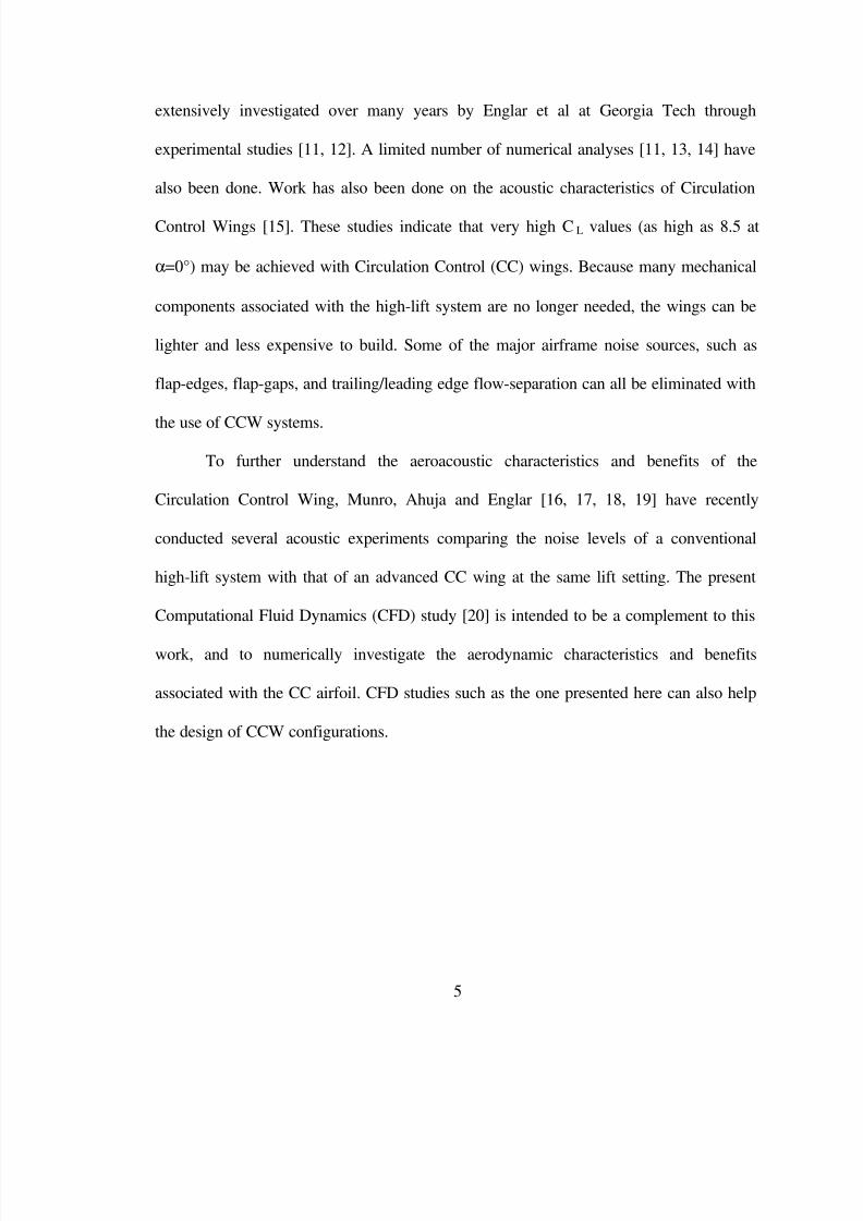
extensively investigated over many years by Englar et al at Georgia Tech through
experimental studies [11, 12]. A limited number of numerical analyses [11, 13, 14] have
also been done. Work has also been done on the acoustic characteristics of Circulation
Control Wings [15]. These studies indicate that very high CL values (as high as 8.5 at
α=0°) may be achieved with Circulation Control (CC) wings. Because many mechanical
components associated with the high-lift system are no longer needed, the wings can be
lighter and less expensive to build. Some of the major airframe noise sources, such as
flap-edges, flap-gaps, and trailing/leading edge flow-separation can all be eliminated with
the use of CCW systems.
To further understand the aeroacoustic characteristics and benefits of the
Circulation Control Wing, Munro, Ahuja and Englar [16, 17, 18, 19] have recently
conducted several acoustic experiments comparing the noise levels of a conventional
high-lift system with that of an advanced CC wing at the same lift setting. The present
Computational Fluid Dynamics (CFD) study [20] is intended to be a complement to this
work, and to numerically investigate the aerodynamic characteristics and benefits
associated with the CC airfoil. CFD studies such as the one presented here can also help
the design of CCW configurations.

7/29/2019 Circulation Control Wing
http://slidepdf.com/reader/full/circulation-control-wing 26/192
6
1.2 Circulation Control Technology
1.2.1 The Circulation Control Wing Concept
Conventional airfoils, such as the NACA series airfoils, all have a sharp trailing
edge. The Kutta condition [21] will be readily satisfied for this kind of the airfoil, and
determines the circulation over the airfoil at a given free-stream condition and angle of
attack. This sharp trailing edge design is very efficient for fixing circulation and lift, and
is widely used both in nature and on man-made lifting surfaces. However, there are two
limitations associated with it. First, the lift generated by a sharp trailing edge airfoil is
only a function of angle of attack, camber, and free-stream conditions, and it can not be
otherwise controlled. Secondly, the maximum lift achieved is limited, because the
adverse pressure gradient on the upper surface eventually causes boundary layer
separation and static stall with the increase in angle of attack. Thus, in order to obtain the
high lift coefficient required during take-off or landing, high-lift devices must be used on
a commercial aircraft. However, a high-lift system always contains many moving parts,
and results in a significant weight penalty, and noise.
The Circulation Control (CC) airfoil overcomes these drawbacks in another way.
It takes advantage of the Coanda effect by blowing a small, high-velocity jet over a
highly curved surface, such as a rounded trailing edge. Since the airfoil trailing edge is
not sharp, the Kutta condition is not fixed and the trailing edge stagnation point is free to
move along the surface. In addition, the upper surface blowing near the trailing edge
energizes the boundary layer, increasing its resistance to separation. With blowing, the
7/29/2019 Circulation Control Wing
http://slidepdf.com/reader/full/circulation-control-wing 27/192
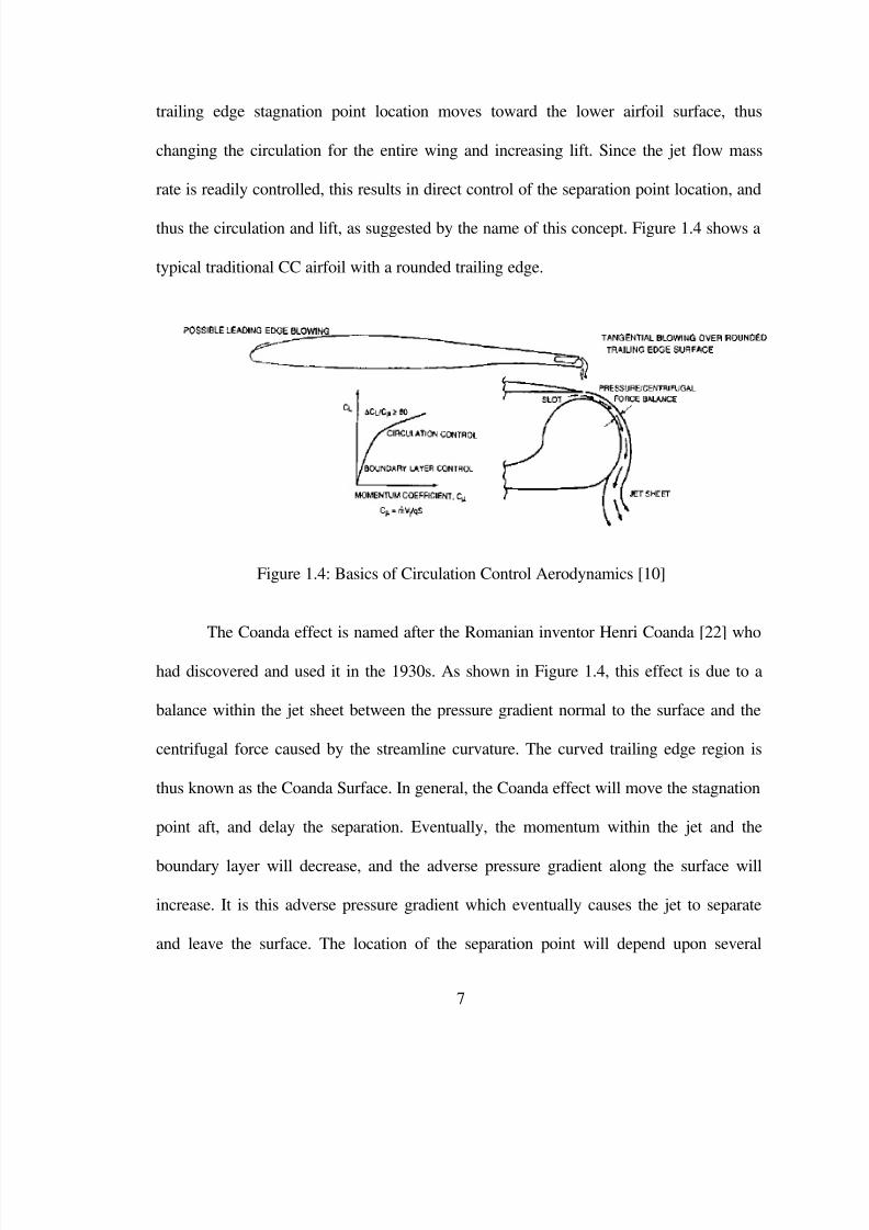
7
trailing edge stagnation point location moves toward the lower airfoil surface, thus
changing the circulation for the entire wing and increasing lift. Since the jet flow mass
rate is readily controlled, this results in direct control of the separation point location, and
thus the circulation and lift, as suggested by the name of this concept. Figure 1.4 shows a
typical traditional CC airfoil with a rounded trailing edge.
Figure 1.4: Basics of Circulation Control Aerodynamics [10]
The Coanda effect is named after the Romanian inventor Henri Coanda [22] who
had discovered and used it in the 1930s. As shown in Figure 1.4, this effect is due to a
balance within the jet sheet between the pressure gradient normal to the surface and the
centrifugal force caused by the streamline curvature. The curved trailing edge region is
thus known as the Coanda Surface. In general, the Coanda effect will move the stagnation
point aft, and delay the separation. Eventually, the momentum within the jet and the
boundary layer will decrease, and the adverse pressure gradient along the surface will
increase. It is this adverse pressure gradient which eventually causes the jet to separate
and leave the surface. The location of the separation point will depend upon several

7/29/2019 Circulation Control Wing
http://slidepdf.com/reader/full/circulation-control-wing 28/192
8
parameters, including the jet momentum coefficient Cµ, the turbulent characteristics of
the jet and the Reynolds number [23]. The jet momentum coefficient Cµ is defined as,
qS
Vm
C
jet
=µ , and will be discussed in the next chapter.
Also as shown in Figure 1.4, at low momentum coefficients, especially when Cµ
is less than 0.01 [23], the tangential blowing will add some energy to the slow moving
flow near the surface. This will delay or eliminate the separation as in conventional
boundary layer control. If the momentum coefficients are high, the lift of the wings will
be increased significantly. The lift augmentation, which is defined as ∆CL / ∆Cµ, and as a
measure of the effectiveness of the blowing in generating lift, can exceed 80. This latter
effect of generating lift via blowing in the manner described above is referred to as
Circulation Control. The Circulation Control concept is superior to boundary layer
control. While boundary layer control aims to eliminate or postpone separation, CC aims
to increase the maximum CL value. This reduces the take-off and landing velocity by a
factor of 2 or so, thereby reducing the runway distance. This is achieved without the
penalty of noise associated with high-lift systems.
The physics of CC airfoils is highly complex and nonlinear. Wood [24], however,
suggests that there are two characteristics of a CC airfoil that determine its performance.
The first is the velocity difference between the jet and the external flow. The second
characteristic is the outer boundary layer momentum deficit. Specifically, Wood also
suggests that the ratio of the jet momentum to outer boundary layer momentum deficit
determines the lift increment due to blowing. Based on this theory and some experimental

7/29/2019 Circulation Control Wing
http://slidepdf.com/reader/full/circulation-control-wing 29/192
9
evidence, Wood predicts that, for low Cµ values, CL varies linearly with Cµ, while for
higher Cµ values, the µ≈ CCL with low free-stream velocities. Eventually, however,
the lift will cease to increase with the momentum coefficient. This phenomenon is known
as jet stall, and is defined as the condition at which ∆CL / ∆Cµ = 0.
1.2.2 The Advanced Circulation Control Airfoil
The earlier designs of the CC airfoils used rounded trailing edges with large
radius to maximize the lift benefit. However, these designs also produced very high drag
[25]. In particular, the high drag associated with the blunt, large radius trailing edge can
be prohibitive under cruise conditions when Circulation Control is no longer necessary.
One way to reduce the drag is to reduce the trailing edge radius. This, however,
causes a loss of lift compared to a large radius configuration. It was also found that the
small radius CC airfoil with larger slot height could cause jet detachment and sudden lift
loss at higher momentum coefficients
[25]. Thus a compromise was needed. The
advanced CC airfoil, i.e., a circulation hinged flap [11, 25, 26], was developed to replace
the original rounded trailing edge CC airfoil.
The advanced CC airfoil developed by Englar is shown in Figure 1.5. The upper
surface of the CCW flap is a large-radius arc surface, but the low surface of the flap is
flat. The flap could be deflected from 0 degrees to 90 degrees. When an aircraft takes-off
or lands, the flap is deflected. Then this large radius on the upper surface produces a large
jet turning angle, leading to a high lift. When the aircraft is in cruise, the flap is retracted
and a conventional sharp trailing edge shape results, greatly reducing the drag. This kind

7/29/2019 Circulation Control Wing
http://slidepdf.com/reader/full/circulation-control-wing 30/192
10
of flap does have some moving elements, which increase the weight and complexity over
an earlier CCW design shown in Figure 1.4. But overall, the hinged flap design still
maintains most of the Circulation Control high lift advantages, while greatly reducing the
drag in cruising condition associated with the rounded trailing edge CCW designs.
Figure 1.5: Dual Radius CCW Airfoil with LE Blowing [10]
The CCW flap is similar to a blown flap. However, it is important to note that
compared to a flat blowing surface in the case of a blown flap, the upper surface is highly
curved for the CCW flap. The curvature is either a curve built from a single radius, or
from multiple radii. A dual-radius configuration is shown in Figure 1.5. The size of the
CCW flap is also much smaller than the blown flap. The governing difference between
CCW flap and the blown flap is that, for CCW flap, there will be a continuously curved
surface downstream of the tangentially blowing jet, and the force modification and high
lift are mainly produced by changes to the jet blowing parameters. On the other hand, for
a blown flap, the surface downstream of the blowing jet is flat, and lift is produced with
the change of the angle of the sharp flap trailing edge or the jet angle relative to the
chord-line.
7/29/2019 Circulation Control Wing
http://slidepdf.com/reader/full/circulation-control-wing 31/192
11
1.2.3 Applications and Benefits of the Circulation Control Wing
Circulation Control technology has many potential applications for both fixed and
rotary wing aircraft, as well as ground vehicles. All of these applications take advantage
of the high lift benefits and the ability of directly controlling the flow field associated
with the CC technology.
For fixed wing vehicles, the high lift generated by CC wings makes them ideal
candidates for short take-off and landing (STOL) and high lift aircraft. To find ways of
improving the aircraft operation from carriers, the Navy sponsored a full-scale flight test
program on an A-6/CCW STOL demonstrator in 1979 [27, 28]. The airfoil used was a
rounded trailing edge CC airfoil. Using only available bleed air from the engines, it could
achieve CL values that were 120% higher than a conventional Fowler flap, or a 140%
increase in the usable lift coefficient at take-off/approach angles of attack. The
researchers were also aware of the drag penalty, and improvements with use of smaller
cylinder trailing edges and hinged flaps have been recommended [25, 29].
For commercial aircraft, compared to a conventional high-lift system, the
advanced CCW flap system can give the same high lift in take-off/landing and small drag
in cruise, but greatly reduce the complexity and weight of the wing. The manufacturing
cost will also be significantly reduced. An experimental and computational study by
Englar et al [11, 12] was conducted to evaluate the effectiveness of applying this concept
to an Advanced Subsonic Transport. As shown in Figure 1.3, a typical wing such as that
found on a Boeing 737 has 15 moving parts. A CCW system, on the other hand, will have
a maximum of 3 components per wing even with leading edge blowing. Using only fan

7/29/2019 Circulation Control Wing
http://slidepdf.com/reader/full/circulation-control-wing 32/192
12
bleed air, the CCW flap will give at least triple the usable lift at taking off and will reduce
the ground roll compared to the conventional high-lift system. Recently, experimental
evaluations were also conducted on the use of blown high-lift devices and control
surfaces on the High Speed Civil Transport (HSCT) aircraft [30]. These studies found
that the advanced pneumatic high-lift devices produced large lift increases as well as
significant drag reductions, and confirmed the effectiveness of combined pneumatic high-
lift devices and control surfaces on these HSCT aircraft.
The ability of controlling the lift directly without angle of attack change gives the
CC airfoil potential of being used on rotary wing aircraft as well. This concept allows the
use of higher harmonic control of helicopters, where cyclic lift variations are usually at
frequencies higher than one per revolution. Suppression of these high frequency
components can result in considerable reduction of rotor vibration, fatigue and noise. In
1979, a CC rotor flight demonstrator based on a Kaman H-2 helicopter was tested [31,
32]. Instead of using a conventional mechanical cyclic and collective blade pitch control
system, a pneumatic aerodynamic and control system was applied. It was found that the
CC rotor had the potential of eliminating the mechanical blade lift and control devices in
hover and forward flight, and also had the ability of achieving higher harmonic control. It
also suggested that the elimination of the angle of attack control could also result in
reducing the hub complexity, number of mechanical parts, size, and drag. However, due
to a control system phasing problem, the flight test envelope was limited.
Another application of the CCW technology is the X-wing stopped rotor aircraft.
In this design, a four-blade CC rotor would be used during vertical take-off and landing,

7/29/2019 Circulation Control Wing
http://slidepdf.com/reader/full/circulation-control-wing 33/192
13
and the rotor assembly would be locked into a stationary position during forward flight,
and function as a fixed wing [33]. Since the wing area was relatively small, the
Circulation Control technology had been used to achieve high lift coefficient during both
the rotary wing and fixed wing modes. Because the rotor blades in such a design need to
be functional both in rotary as well as in fixed forward flight mode, they must be fore-
and-aft symmetrical. CC airfoils, with their rounded leading and trailing edges, are
ideally suited to this application. During the rotary wing mode, as mentioned above, the
cyclic variation of the lift coefficient may be controlled by variation of the jet momentum
coefficient, rather than pitching motion. This concept was tested full-scale in the NASA
Ames wind tunnel and successfully completed the transition from hover to forward flight.
Besides these applications in flying vehicles, a number of non-flying applications
have also been investigated, where the Circulation Control technology was used to
modify or control the flow field around moving objects. One investigation by Englar [34]
is to improve the performance, economics and safety of heavy vehicles (i.e. large
tractor/trailer trucks). There are many other potential applications for the Circulation
Control or Pneumatic Aerodynamic technology besides these mentioned above. The
reader is strongly referred to the Reference [10], which summarizes many of this effort
from beginning to the year 2000.

7/29/2019 Circulation Control Wing
http://slidepdf.com/reader/full/circulation-control-wing 34/192
14
1.3 Previous Research Work
Circulation Control research based on the Coanda effect originates back in the
1930s [22]. Because of the great benefits of the Circulation Control technology, many
experimental and numerical studies have since then been done to investigate the
characteristics and performance of CC airfoils.
The early research work was done in England. Cheeseman et al [35] applied
blowing to helicopter rotors. Kind [36] gave a simplified calculation method for
Circulation Control by tangential blowing around a bluff trailing edge. After 1970, this
concept was pursued in the United States by Navy researchers. The David Taylor Naval
Ship Research and Development Center (DTNSRDC) became a major center for
Circulation Control research. Experiments by Williams and Howe [37], Englar [38, 39],
Abramson [40], Abramson and Rogers [41], and others examined the effect of a wide
range of parameters on Circulation Control airfoils, including geometric factors such as
the thickness, camber, angle of attack, and free-stream conditions such as Mach number.
For a summary of this research work for the years 1969 through 1983, the reader is
referred to Reference [42]. This work by Englar et al also provides a summary of CC-
related research conducted by other agencies outside the Navy.
In addition to these basic aerodynamic experiments, recently, many studies have
been focused on CCW applications for the rotary and fixed wing aircraft. Some of the
studies were mentioned in section 1.2.3, and Reference [10] gives a detailed description
of many such studies made until the year 2000.

7/29/2019 Circulation Control Wing
http://slidepdf.com/reader/full/circulation-control-wing 35/192
15
Compared to so many aerodynamic studies, however, the acoustic studies for the
CCW are very limited. Salikuddin, Brown and Ahuja [15] experimentally examined the
changes in noise produced by an upper surface with and without blowing. Carpenter et al
[43] have experimentally investigated the noise emitted from supersonic jet flows over
axisymmetric Coanda surfaces. Howe [44] recently analytically studied the noise
generated by a hydrofoil with a Coanda wall jet Circulation Control device. Munro and
Ahuja [16, 17, 18, 19] compared the noise characteristics of a CC wing and a
conventional flap wing at the same lift setting, and studied the fluid dynamics and
aeroacoustics of a high aspect-ratio jet. It was found that a CC wing had a significant
acoustic advantage over a conventional wing for the same lift performance.
There have only been a limited number of computational studies of CCW
configurations. In the earliest studies, panel methods combined with boundary layer
analysis and wall jet models were used. Some good results were obtained by using a
potential flow solver developed by Dvorak et al [45, 46], but the solutions did not appear
to have the accuracy needed for CC airfoil designs.
Determining the performance of CC airfoils using analytical or numerical
methods has proven to be extremely difficult due to the viscous flow region that needs to
be modeled. The flow over a CC airfoil is greatly complicated by the rounded trailing
edge or Coanda surface, and the introduction of the jet blowing. There are strong
interactions between the jet region and the overall flow due to circulation coupling. An
accurate analysis of the flow field requires a procedure that accounts for this highly-
coupled nature of the viscous and inviscid flow regions. This could not be done by the

7/29/2019 Circulation Control Wing
http://slidepdf.com/reader/full/circulation-control-wing 36/192
16
simple potential methods until the 1980s. Due to this highly-coupled, nonlinear viscous
behavior of the flow field, the Navier-Stokes equations present the best prospects of
modeling this problem. However, even the Navier-Stokes methods are challenged due to
the lack of accurate turbulence models for highly curved flows with strong adverse
pressure gradients.
Many numerical studies were conducted during the 1980s, which examined the
possibility of using Navier-Stokes equations to predict the characteristics of CC airfoils.
Berman [47] of DTNSRDC computed the flow over the aft 50% chord of a CC airfoil
using a MacCormack explicit solver with the Baldwin-Lomax turbulence model [48]. The
results showed trends consistent with the experiments. However, the magnitudes of the
computed pressure coefficients were not as large as those found experimentally. Pulliam
et al. [49] also employed an implicit formulation of the Navier-Stokes equations with the
Baldwin-Lomax turbulence model to compute the flow over CC airfoils. Their results
faithfully reproduced the experimental results of Abramson and Rogers [41] for the
higher blowing rates, although they also concluded that better turbulence models were
needed. Viegas et al [50] computed the flow field over the trailing edge of the CC airfoil
used in the experiment of Spaid and Keener [51], and a good agreement with the
measured pressure distribution was also obtained. Shrewsbury [52, 53, 54] of Lockheed
Martin used an implicit formulation of the compressible Reynolds-average Navier-Stokes
equations (RANS) with a modified form of the Baldwin-Lomax turbulence model. The
turbulence model included a correction by Bradshaw [55] to account for the curvature of
the Coanda surface. This method performed well and provided lift and pressure

7/29/2019 Circulation Control Wing
http://slidepdf.com/reader/full/circulation-control-wing 37/192
17
distribution results in close agreement with the experimental data. Shrewsbury [53] also
concluded that better turbulence models were needed to more accurately calculate the
flow field characteristics around CC airfoils. These studies have demonstrated that the
Navier-Stokes equations can indeed provide good estimates of the lift, pressure
distribution, and pitch moments of CC airfoils at various flight conditions provided the
turbulence model is able to give a reasonable good estimate of the jet separation point
from the Coanda surface.
More recently, the solutions of Navier-Stokes equations have also been used to
predict the static and dynamic performance of CC airfoils. Shrewsbury [13, 14, 56]
conducted a study of an oscillating CC airfoil to determine the dynamic stall
characteristics. Williams and Franke [57] also developed a computational procedure
based on Navier-Stokes equations to predict the aerodynamic performance of a CC airfoil
for a range of jet blowing rates. The results were shown to be dependent on an empirical
curvature constant in the Baldwin-Lomax turbulence model to account for the curved
flow over the blunt trailing edge, and the development of accurate turbulence models for
CC airfoils was also recommended. Linton [58] computed the post jet-stall behavior of a
CC airfoil using a fully implicit Navier-Stokes code and the Baldwin-Lomax and κ -ε
turbulence models. Numerical solutions for the stalled and unstalled flow over a CC
airfoil were obtained, and it was found that the post-stall behavior of a CC airfoil was a
highly regular periodic oscillation. Liu et al [59] investigated the unsteady flow around a
CC airfoil with a Navier-Stokes method. The calculations included the flow around a CC
airfoil with a pulsating jet, the flow around an oscillating CC airfoil, and the flow around
7/29/2019 Circulation Control Wing
http://slidepdf.com/reader/full/circulation-control-wing 38/192
18
an oscillating airfoil with pulsed jet. Wang and Sun [60] also studied the Circulation
Control with multi-slot blowing. It was found that at small and medium Cµ, the multi-slot
CC blowing could increase the lift of the airfoil and reduce the amount of the energy
expenditure, so that it could improve the aerodynamic performance of CC airfoils at
higher Mach number by avoiding the “compressibility stall”. All of above studies were
based on the traditional rounded trailing edge CC airfoils. For the advanced small hinge-
flap CC airfoil, Smith et al [61] calculated the pressure coefficient distribution over a
dual-radius CC airfoil with aft CCW flap at 900 and Krueger flap at 600. The agreement
with the experimental data was quite good.
Around 2000, thanks to great improvements in computer speed, more complicated
and accurate methods began to be used to numerically investigate the Circulation Control
or separation control phenomena. Slomski et al [62] investigated the influence of
turbulence models on the performance of CC airfoils. Instead of using the traditional
Baldwin-Lomax model, three advanced turbulence models were used: the standard κ -
ε model, the modified κ -ε model, and a full Reynolds stress model. It was found that for
small Cµ, the κ -ε and modified κ -ε turbulence models could predict the lift generated by
the CC airfoil reasonably well. However, at higher Cµ, only the Reynolds stress
turbulence model could capture the physics of the Circulation Control problem, allowing
a reasonable prediction of the lift. Large-eddy Simulation (LES) [63] and Direct
Numerical Simulation (DNS) [64] methods have also been reported in last two years,
primarily for the numerical investigation of boundary layer separation control.

7/29/2019 Circulation Control Wing
http://slidepdf.com/reader/full/circulation-control-wing 39/192
19
1.4 Overview of the Present Work
The main objectives of the current study are to numerically investigate the
aerodynamic characteristics and benefits of Circulation Control Airfoils/Wings. The
present study is aimed at understanding the physical phenomena associated with the CC
concept, and at extending these 2-D studies to 3-D applications, and to pulsed jet
configurations. Specifically this work is aimed at answering the following questions,
which have not been fully numerically investigated to the knowledge of the author:
SCan pulsed jets be used to replace steady blowing to generate the same high lift
with relative lower mass flow rate? If so, what is the optimum value for jet
blowing coefficient Cµ, pulsed jet frequency, wave shape and duty cycle? What
are the benefits and drawbacks of pulsed jets relating to steady jets?
SIn many instances, it may be desirable to retrofit an existing wing with Circulation
Control. What are the aerodynamic benefits and drawbacks? For example, can the
vortices generated at flap edges be reduced in strength or altogether eliminated
using Circulation Control and why? Can the tip vortex of a wing be weaken or
eliminated by jet blowing over the rounded wing tip?
Of course these issues can, and should also be, studied in good quality wind
tunnels. CFD provides a powerful way of taking a first look at the problems before an
experiment is designed. Thus it is hoped that one of the benefits of this work will be a
comprehensive matrix of calculations that will assist the experimental aerodynamics
researchers in designing the experiments.

7/29/2019 Circulation Control Wing
http://slidepdf.com/reader/full/circulation-control-wing 40/192
20
The CC airfoil configuration used in present study is the advanced hinge-flap CC
wing tested in References [9, 11, 12] and [16, 17, 18, 19]. This configuration was chosen
for the following reasons. This design is proven to be aerodynamically highly beneficial
during both take-off/landing and cruise conditions, and also less noisy than a
conventional high-lift system. An extensive set of experimental data for the two-
dimensional steady blowing is available for comparison and validation.
The rest of this thesis is organized as follows. In Chapter II, the mathematical and
numerical formulation of the governing equations is presented. It also includes the
mathematical representation of the turbulence models. The initial and boundary
conditions, which include the jet exit slot boundary condition, are addressed at the end of
Chapter II. The numerical results for the two-dimensional steady blowing are presented
in Chapter III. It includes a validation study for a NACA0012 wing, and comparisons
with the experimental measurements for steady jets. The effects of several parameters on
the static performance of the CC airfoil are also included. Simulations of the use of
pulsed jets on CCW configurations are given in Chapter IV. In particular, the wave form
and frequency effects on pulsed jet performance are discussed. Some preliminary results
for three-dimensional Circulation Control wing simulations are presented in Chapter V.
They include effects of tangential blowing on a wing-flap configuration to eliminate the
flap-edge vortex, and a spanwise blowing over a rounded wing tip to control the tip
vortex. Finally, the conclusions and recommendations for the further improvement of the
CC technology studies are given in Chapter VI.
7/29/2019 Circulation Control Wing
http://slidepdf.com/reader/full/circulation-control-wing 41/192
21
CHAPTER II
MATHEMATICAL AND NUMERICAL FORMULATION
In order to analyze the flow field around the Circulation Control Airfoils/Wings,
solution of two-dimensional or three-dimensional Navier-Stokes equations is required.
Because of the complexity of wing/airfoil configurations and the strong viscous effects, it
is impossible to obtain an analytical solution of the Navier-Stokes equations for practical
configurations. Thus numerical techniques have to be used to solve those equations. In
this chapter, the governing equations and the numerical procedures employed in the
present study are documented. The formulation given below has been applied to many
fixed wing and rotorcraft studies by Sankar and his co-workers [65, 66, 67, 68].
In section 2.1, the governing equations for the three-dimensional unsteady
compressible flow are presented in Cartesian coordinates and Curvilinear coordinates
separately. The numerical discretization procedure and the alternating directing implicit
(ADI) scheme used to solve the governing equations are given in section 2.2. The
turbulence models used in the present study are discussed in section 2.3. Finally the
initial conditions, boundary conditions, and the special jet slot boundary condition
applied to the solver are described in section 2.4.

7/29/2019 Circulation Control Wing
http://slidepdf.com/reader/full/circulation-control-wing 42/192
22
2.1 The Governing Equations
Navier-Stokes equations are a set of partial differential equations for the
conservation of mass, momentum, and energy. These may be derived by applying the
principle of classical mechanics and thermodynamics. These equations are based on
Newton’s hypothesis, that the normal and shear stresses are linear functions of the rates
of deformation, and that the thermodynamic pressure is equal to the negative of one-third
the sum of the normal stresses.
2.1.1 Governing Equations in Cartesian Coordinates
The divergence form of three-dimensional compressible Navier-Stokes equations
in Cartesian coordinates without external body forces or outside heat addition can be
written as [69]:
zyxzyxt ∂∂+
∂∂+
∂∂=
∂∂+
∂∂+
∂∂+
∂∂ TSRGFEq (2.1)
Here q is the flow vector or the unknown flow variables, which include the density and
velocities. E, F and G are the inviscid flux vectors and R, S and T are the viscous flux
vectors in the x, y and z directions, respectively.

7/29/2019 Circulation Control Wing
http://slidepdf.com/reader/full/circulation-control-wing 43/192
23
The flow vector and the inviscid flux terms are:
ρ
ρ
ρ
ρ
=
tE
w
v
u
q
+
ρ
ρ
+ρ
ρ
=
u)pE(
uw
uv
pu
u
t
2
E
+
ρ
+ρ
ρ
ρ
=
v)pE(
vw
pv
uv
v
t
2F
+
+ρ
ρ
ρ
ρ
=
w)pE(
pw
uw
uw
w
t
2
G
(2.2)
Here, E t is the total energy, and it can be expressed as:
+++ρ= )wvu(
2
1TCE 222
vt (2.3)
In above equations, the density ρ , the velocity components (u, v, w) in the ( x, y, z)
directions and total energy E t are the unknown flow parameters. The pressure is related to
the total energy and velocities by the following equations:
RTp ρ= (2.4)
and:
++ρ−−γ = )wvu(
2
1E)1(p 222
t (2.5)

7/29/2019 Circulation Control Wing
http://slidepdf.com/reader/full/circulation-control-wing 44/192
24
In Equation (2.5), γ is the specific heat ratio. Since the working fluid is air, a value of 1.4
is used.
The viscous terms in equation (2.1) are:
τ
τ
τ
=
5x
xz
xy
xx
E
0
R ,
τ
τ
τ
=
5y
yz
yy
yx
E
0
S ,
τ
τ
τ
=
5z
zz
zy
zx
E
0
T (2.6)
As stated earlier, the Newtonian fluid assumption has been made to link the stress
tensor with the pressure and velocity components [70]. Then the following relations can
be obtained:
3,2,1 j,ixu
xu
xu
quE
ij
k
k
i
j
j
iij
iij j5i
=δ∂∂λ+
∂∂+∂∂µ=τ
−τ=
(2.7)
where δ ij is the Kronecker delta function; Subscripts “1, 2, 3” represent the tensors in the
x, y, and z directions. The effect of fluid compressibility is expressed by the dilatation
term in conjunction with the second coefficient of viscosity λ . In the current study, the
fluid is assumed to be in a state of local thermodynamic equilibrium [71], i.e., Stoke’s
hypothesis [72] is used to relate the first and second viscosity coefficients in the above
equation (2.7). Thus,

7/29/2019 Circulation Control Wing
http://slidepdf.com/reader/full/circulation-control-wing 45/192
25
µ−=λ3
2 (2.8)
The stress terms and heat transfer terms in equation (2.6) can now be written as follows:
∂
∂−
∂∂
−∂∂
µ=τ
∂∂
+∂∂
µ=τ
∂∂−
∂∂−
∂∂µ=τ
∂∂
+∂∂
µ=τ
∂∂
+∂∂
µ=τ
∂∂
−∂∂
−∂∂
µ=τ
y
v
x
u
z
w2
3
2
y
w
z
v
z
w
x
u
y
v2
3
2
x
w
z
u
x
v
y
u
z
w
y
v
x
u2
3
2
zz
yz
yy
xz
xy
xx
(2.9)
xxzxyxx5x qwvuE +τ+τ+τ=
yyzyyxy5y qwvuE +τ+τ+τ=
zzzyzxz5z qwvuE +τ+τ+τ=
(2.10)
Under local equilibrium conditions, Fourier’s law [73] is used to relate the heat transfer
rates q x , q y and q z with the temperature gradient:

7/29/2019 Circulation Control Wing
http://slidepdf.com/reader/full/circulation-control-wing 46/192
26
z
Tk q
y
Tk q
x
Tk q
z
y
x
∂∂−=
∂∂
−=
∂∂
−=
(2.11)
The thermal conductivity, k , can be related to the molecular viscosity using the
kinetic theory of gases [74]:
Pr
C
Pr
Ck VP µγ
=µ
= (2.12)
where C p is the specific heat at constant pressure. For a calorically perfect gas, it is a
constant and defined as1
RCP −γ
γ = . Here R is the gas constant and γ is the specific heat
ratio, which is equal to 1.4 for air. Furthermore, Pr is the Prandtl number; and Pr = 0.72
for air.
The local speed of sound is given by:
( ) ( )
++−
ρ−γ γ =γ = 222t wvu
2
1E1RTa (2.13)
In numerical simulations, it is convenient if all quantities in the Navier-Stokes
equations are non-dimensionalized by some reference values. The advantage in doing
this is that the number of parameters in the flow reduces to a few, such as Mach number,

7/29/2019 Circulation Control Wing
http://slidepdf.com/reader/full/circulation-control-wing 47/192
27
Reynolds number, and Prandtl number. Also, by non-dimensionalizing the equations, the
flow variables will be of the order of O(1).
The following reference values have been used in the present studies:
etemperaturFreestream,TT
itycosvisFreestream,
densityFreestream,
soundof speedFreestream,aV
airfoiltheof ChordL
ref
ref
ref
ref
ref
∞
∞
∞
∞
=
µ=µ
ρ=ρ
=
=
(2.14)
The non-dimensional flow variables are expressed as follows:
2
ref ref
t*
t
ref
*
2
ref ref
*
ref
*
ref
*
ref
*
ref
*
ref
*
ref ref
*
ref
*
ref
*
ref
*
V
EE
T
TT
V
pp
V
ww
V
vv
V
uu
V / L
tt
L
zz
L
yy
L
xx
ρ==
ρ=
ρρ
=ρ
µµ
=µ===
====
(2.15)
where the non-dimensional variables are denoted by an asterisk.
Substituting the non-dimensional variables in equation (2.15) into the equation
(2.1), an equation very similar to (2.1) is obtained, but there are two non-dimensional
coefficients that appear in front of the inviscid and viscous terms. These coefficients are
the Mach number and Reynolds number, which are defined as follows:
∞
∞∞
∞
∞∞ µ
ρ=
γ = ref
L
LVRe
RT
VM
ref (2.16)

7/29/2019 Circulation Control Wing
http://slidepdf.com/reader/full/circulation-control-wing 48/192
28
For a detailed description and expression of the non-dimensional equations, the reader is
referred to Reference [69]. In the following discussions, all variables (ρ , u, v, p etc) are
non-dimensional. The asterisk has been dropped for convenience.
2.1.2 Governing Equations in Curvilinear Coordinates
To obtain solutions for the flow past arbitrary geometries and handle arbitrary
motions, a body-fitted coordinate system is desired so that the boundary surfaces in the
physical plane can be easily mapped onto planes or lines in the computational domain.
The compressible Navier-Stokes equations can be written in terms of a generalized non-
orthogonal curvilinear coordinate system ( ξ ,η , ζ ) using the generalized transformation
described in Appendix A:
t
)t,z,y,x(
)t,z,y,x(
)t,z,y,x(
=τ
ζ=ζ
η=η
ξ=ξ
(2.17)
Applying the transformation to the equation (2.1), the following non-dimensional
governing equations in the curvilinear coordinate system can be obtained.
)ˆˆˆ
(Re
Mˆˆˆˆ ςηξ
∞
ςηξτ ++=+++ TSRGFEq (2.18)
Here,

7/29/2019 Circulation Control Wing
http://slidepdf.com/reader/full/circulation-control-wing 49/192
29
ρρρρ
=
e
w
v
u1
ˆJ
q (2.19)
J is the Jacobian of transformation, and it is given by:
)zxzx(y)zxzx(y)zxzx(y
1
ηξξηςξςςξηςηηςξ −+−+−=J (2.20)
The quantities GFE ˆ,ˆ,ˆ and TSR ˆ,ˆ,ˆ are related to their counterparts E, F, G, and R, S, T
as follows:
( )tzyx
1ˆ ξ+ξ+ξ+ξ= qGFEJ
E
( )tzyx1ˆ η+η+η+η= qGFEJ
F
( )tzyx
1ˆ ζ+ζ+ζ+ζ= qGFEJ
G
( )zyx
1ˆ ξ+ξ+ξ= TSRJ
R
( )zyx
1ˆ η+η+η= TSR
J
S
( )zyx
1ˆ ζ+ζ+ζ= TSRJ
T
(2.21)

7/29/2019 Circulation Control Wing
http://slidepdf.com/reader/full/circulation-control-wing 50/192
30
In numerical simulations, the contravariant velocities U , V , and W are used as the
velocity components in the generalized coordinates, which are related to the original
velocities (u,v and w) as:
zyxt
zyx
wvu
)zw()yv()xu(U
ξ+ξ+ξ+ξ=
ξ−+ξ−+ξ−= τττ
zyxt
zyx
wvu
)zw()yv()xu(V
η+η+η+η=
η−+η−+η−= τττ
zyxt
zyx
wvu
)zw()yv()xu(W
ζ+ζ+ζ+ζ=
ζ−+ζ−+ζ−= τττ
(2.22)
where:
zyxt
zyxt
zyxt
zyx
zyx
zyx
ς−ς−ς−=ς
η−η−η−=η
ξ−ξ−ξ−=ξ
τττ
τττ
τττ
(2.23)
The contravariant velocity components U, V and W are in directions normal to the
constant ζηξ and, surfaces, respectively. The quantity ( xτ , yτ and zτ ) is the velocity of
any points on the “grid” in an initial frame. In the present work, the body is not in motion
and these velocities are zero.
The inviscid GFE ˆ,ˆ,ˆ and viscous TSR ˆ,ˆ,ˆ flux vectors in the transformed
coordinate system are:
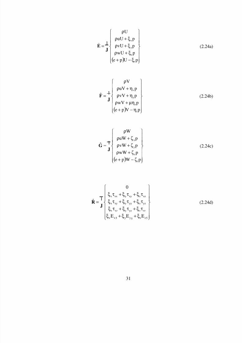
7/29/2019 Circulation Control Wing
http://slidepdf.com/reader/full/circulation-control-wing 51/192
31
( )
ξ−+
ξ+ρξ+ρξ+ρ
ρ
=
pUpe
pwU
pvU
puU
U
1
t
z
y
x
JE (2.24a)
( )
η−+µη+ρη+ρη+ρ
ρ
=
pVpe
pwV
pvV
puV
V
1ˆ
t
z
y
x
JF (2.24b)
( )
ζ−+ζ+ρζ+ρζ+ρ
ρ
=
pWpe
pwW
pvW
puW
W
1ˆ
t
z
y
x
JG (2.24c)
ξ+ξ+ξτξ+τξ+τξτξ+τξ+τξτξ+τξ+τξ
=
5zz5yy5xx
zzzyzyxzx
yzzyyyxyx
xzzxyyxxx
EEE
0
1ˆJ
R (2.24d)

7/29/2019 Circulation Control Wing
http://slidepdf.com/reader/full/circulation-control-wing 52/192
32
η+η+ητη+τη+τητη+τη+τη
τη+τη+τη
=
5zz5yy5xx
zzzyzyxzx
yzzyyyxyx
xzzxyyxxx
EEE
0
1ˆJ
S (2.24e)
ζ+ζ+ζτζ+τζ+τζτζ+τζ+τζ
τζ+τζ+τζ
=
5zz5yy5xx
zzzyzyxzx
yzzyyyxyx
xzzxyyxxx
EEE
0
1ˆJ
T (2.24f)
The viscous flux terms with the shear stresses in the transformed coordinates are:
( )[ ]
( )[ ]
( )[ ]
)wwwvvv(
)wwwuuu(
)vvvuuu(
)vvv()uuu(www23
2
)www()uuu(vvv23
2
)www()vvv(uuu232
yyyzzzyz
xxxzzzxz
xxxyyyxy
yyyxxxzzzzz
zzzxxxyyyyy
zzzyyyxxxxx
ζ+η+ξ+ζ+η+ξµ=τ
ζ+η+ξ+ζ+η+ξµ=τ
ζ+η+ξ+ζ+η+ξµ=τ
ζ+η+ξ−ζ+η+ξ−ζ+η+ξµ=τ
ζ+η+ξ−ζ+η+ξ−ζ+η+ξµ=τ
ζ+η+ξ−ζ+η+ξ−ζ+η+ξµ=τ
ζηξζηξ
ζηξζηξ
ζηξζηξ
ζηξζηξζηξ
ζηξζηξζηξ
ζηξζηξζηξ
(2.25)
where the Stokes hypothesis for bulk viscosity has been used, as discussed earlier.

7/29/2019 Circulation Control Wing
http://slidepdf.com/reader/full/circulation-control-wing 53/192
33
The auxiliary functions are:
( )
∂ζ∂
ζ+∂η∂
η+∂ξ∂
ξ−γ
µ+τ+τ+τ=
2
x
2
x
2
xxzxyxx5x
aaa
1PrwvuE
( )
∂ζ∂
ζ+∂η∂
η+∂ξ∂
ξ−γ
µ+τ+τ+τ=
2
y
2
y
2
yyzyyxy5y
aaa
1PrwvuE
( )
∂ζ∂
ζ+∂η∂
η+∂ξ
∂ξ
−γ µ
+τ+τ+τ=2
z
2
z
2
zzzyzxz5z
aaa
1PrwvuE
(2.26)
The quantities ξ x, ξ y, ξ z etc. are called the metrics of transformation, Pr is Prandtl
number, a is the speed of sound, and a2
= γ RT . γ is the specific heat ratio and a value of
1.4 has been given for air. Those values can be earlier computed on a body fitted grid
[69], as discussed later.
The time derivativeτ∂
∂in the transformed plane is related to the time derivative in
the physical planet∂∂ as follows:
ς∂∂
ς+η∂∂
η+ξ∂
∂ξ+
τ∂∂
=∂∂
ςηξttt
,,z,y,xt (2.27)
with ξ t , ηt and ζ t appropriately defined as shown in equation (2.23). If the body is not
moving, or the grid is not moving,τ∂
∂=
t∂∂
.

7/29/2019 Circulation Control Wing
http://slidepdf.com/reader/full/circulation-control-wing 54/192
34
2.2 Numerical Procedure
The governing equations (2.1) can be solved analytically only for some very
simple cases. For most aerodynamic applications, the equations have to be solved
numerically. There are two major approaches to solve these equations numerically in
Computational Fluid Dynamics (CFD). One is the Finite Difference method, in which the
governing equations in the continuous domain are transformed into a computational
domain with uniform grid spacing and then discretized. The second is the Finite Volume
method, in which the conservation principles are applied to a fixed region in physical
space known as a control volume. The governing equations are thus represented in
integral forms for finite volume method, which are discretized directly in the physical
domain.
In the present work, a semi-implicit finite difference scheme based on the
Alternating Direction Implicit (ADI) [75, 76, 77] method was used. A brief description of
this finite difference scheme will be given in this section. For a detailed review of the
development of the finite difference scheme and the ADI method, the reader is referred to
the Reference [78].
2.2.1 Temporal Discretization
The unsteady compressible Navier-Stokes equations are a mixed set of
hyperbolic-parabolic equations. Since the governing equations are parabolic in time, they
may be solved with advancing in time using a stable, dissipative scheme. Because of the

7/29/2019 Circulation Control Wing
http://slidepdf.com/reader/full/circulation-control-wing 55/192
35
time step restriction from stability considerations for the explicit method, an implicit
first-order accurate scheme is used:
)(Oˆ
ˆˆ
1n
n1n
τ∆+τ∂
∂
τ∆+=
++ q
qq (2.28)
Here, the superscript ‘n+1’ represents the new, or unknown time level, and the
superscript ‘n’ represents the previous, or known time level. A second order scheme
could also have been used, but the first-order scheme gives better stability properties. If
the time step is small enough to maintain the stability for Navier-Stokes equations, a
satisfactory temporal accuracy is still achieved.
The Navier-Stokes equation (2.18) then can be written in a semi-discrete form as:
n1n1n
)ˆˆˆ(Re
M)ˆˆˆ(
ˆTSRGFE
qζηξ
∞+
ζηξ
+
δ+δ+δ+δ+δ+δ−=τ∂
∂
(2.29)
where, for example, Eξδ is a numerical approximation to the derivative ξ∂∂E , and
standard fourth-order or second-order central differencing is used to calculate these
derivatives. The viscous terms are evaluated explicitly by using the old time level values,
and added to the right-hand side of the equation. The details of the spatial discretization
procedure will be discussed later.
Substitute equation (2.29) into equation (2.28), the following equation is obtained:
)ˆˆˆ(Re
M)ˆˆˆ(ˆˆ
nnn1n1n1nn1n
TSRGFEqq ζηξ∞+
ζ+
η+
ξ+
δ+δ+δτ∆+δ+δ+δτ∆−= (2.30)

7/29/2019 Circulation Control Wing
http://slidepdf.com/reader/full/circulation-control-wing 56/192
36
Note that the inviscid terms are at the new time level ‘n+1’ (or treated implicitly),
while the viscous terms are explicitly computed using known information at the old time
level ‘n’. For this reason, this approach is a semi-implicit scheme.
2.2.2 Linearization of the Difference Equations
Because the flux vectors E , F , and G are nonlinear, the algebraic equations
shown in (2.30) for the unknown vector, 1n+q , are nonlinear. However, this non-linearity
may be removed, while maintain the temporal accuracy, by using a linearization
procedure. In the present study, following the method proposed by Beam and Warming
[79], those nonlinear flux vectors are linearized about the non-linear solution at an earlier
time level ‘n’ as follows:
)(O)ˆˆ]([ˆˆ
)(O)ˆˆ]([ˆˆ
)(O)ˆˆ]([ˆˆ
2n1nnn1n
2n1nnn1n
2n1nnn1n
τ∆+−+=
τ∆+−+=
τ∆+−+=
++
++
++
qqCGG
qqBFF
qqAEE
(2.31)
where [A], [B] and [C] are the Jacobian matrices:
q
GC
q
FB
q
EA
ˆ
ˆ][and
ˆ
ˆ][
ˆ
ˆ][
∂∂
=∂∂
=∂∂
= (2.32)
For the Euler equations, these 5*5 matrices can be evaluated analytically and are
given by Pulliam [80]. The viscous terms are modeled explicitly, and no linearization is
needed.

7/29/2019 Circulation Control Wing
http://slidepdf.com/reader/full/circulation-control-wing 57/192
37
The detailed forms of those matrices are shown below:
σθ+ξθσ−ξθσ−ξθσ−ξ−φθσξ−γ ξ−Θσξ−ξσξ−ξθ−φξσξσξ−ξ−γ ξ−Θσξ−ξθ−φξ
σξσξ−ξσξ−ξ−γ ξ−Θθ−φξξξξξ
=
tzyx
2
zzzyzx
2
z
yyzyyx2
y
xxzxyx
2
x
zyxt
wEvEuE)E(
w)2(vwuww
wvv)2(uvv
wuvuu)2(u
0
][A (2.33)
where:
2
t
zyx
2222
eE
1
wvu
2 / )wvu)(1(
φ−ργ
=
θ+ξ=Θ
−γ =σ
ξ+ξ+ξ=θ
++−γ =φ
(2.34)
The matrices [B] and [C] may be similarly conducted if η and ζ are used in the above
equations, respectively, instead of ξ .
After substituting the linearized flux vectors equations (2.31) into (2.30), the
following systems of linear equations for 1n+q can be achieved:
nn1nnnn )ˆˆ)]((+[ RHSqqCBAI =−δ+δ+δτ∆ +ζηξ (2.35)
The RHS in above equation is the steady state portion of the governing equations,
and is known as the “residual”. For Navier-Stokes calculations, the residual is given by:
)ˆˆˆ(Re
M)ˆˆˆ( nnnnnnn TSRGFERHS ζηξ
∞ζηξ δ+δ+δτ∆+δ+δ+δτ∆−= (2.36)
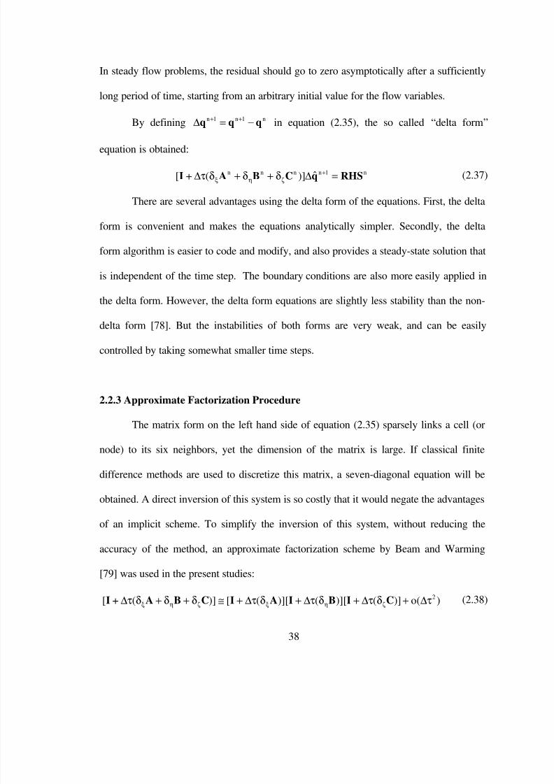
7/29/2019 Circulation Control Wing
http://slidepdf.com/reader/full/circulation-control-wing 58/192
38
In steady flow problems, the residual should go to zero asymptotically after a sufficiently
long period of time, starting from an arbitrary initial value for the flow variables.
By defining n1n1nqqq −=∆ ++ in equation (2.35), the so called “delta form”
equation is obtained:
n1nnnn ˆ)](+[ RHSqCBAI =∆δ+δ+δτ∆ +ζηξ (2.37)
There are several advantages using the delta form of the equations. First, the delta
form is convenient and makes the equations analytically simpler. Secondly, the delta
form algorithm is easier to code and modify, and also provides a steady-state solution that
is independent of the time step. The boundary conditions are also more easily applied in
the delta form. However, the delta form equations are slightly less stability than the non-
delta form [78]. But the instabilities of both forms are very weak, and can be easily
controlled by taking somewhat smaller time steps.
2.2.3 Approximate Factorization Procedure
The matrix form on the left hand side of equation (2.35) sparsely links a cell (or
node) to its six neighbors, yet the dimension of the matrix is large. If classical finite
difference methods are used to discretize this matrix, a seven-diagonal equation will be
obtained. A direct inversion of this system is so costly that it would negate the advantages
of an implicit scheme. To simplify the inversion of this system, without reducing the
accuracy of the method, an approximate factorization scheme by Beam and Warming
[79] was used in the present studies:
)(o)]()][()][([)](+[ 2τ∆+δτ∆+δτ∆+δτ∆+≅δ+δ+δτ∆ ζηξζηξ CIBIAICBAI (2.38)

7/29/2019 Circulation Control Wing
http://slidepdf.com/reader/full/circulation-control-wing 59/192
39
This factorization method has not reduced the temporal accuracy of the method,
but it has changed a large, sparse matrix into the product of three easily inverted
tridiagonal matrices. Thus, the computational efficiency is greatly increased.
After the approximate aactorization (AF) procedure, the system equations for
1nq +∆ are solved by three successive block-tridiagonal inversions:
21nn
12n
n1n
ˆˆ)]([
ˆˆ)]([
ˆ)]([
qqCI
qqBI
RHSqAI
∆=∆δτ∆+
∆=∆δτ∆+
=∆δτ∆+
+ζ
η
ξ
(2.39)
2.2.4 Spatial Discretization of the Inviscid Terms
The right hand side of equation (2.37), nRHS , contains inviscid derivative terms
such as Eξδ , where E includes the flux of mass, momentum and energy, and viscous
terms such as Rξδ . To numerically model those derivatives, a spatial discretization is
required.
For those inviscid terms, a standard second or fourth order central differencing is
used.
Second Order:ξ∆
−=δ −+
ξ2
ˆˆˆ k , j,1ik , j,1i EEE (2.40a)
and
Fourth Order:ξ∆
+−+−=δ −−++
ξ12
ˆˆ8ˆ8ˆˆ k , j,2ik , j,1ik , j,1ik , j,2i EEEEE (2.40b)

7/29/2019 Circulation Control Wing
http://slidepdf.com/reader/full/circulation-control-wing 60/192
40
It is possible to obtain fourth-order spatial accuracy without increasing the coding
work too much, while preserving the block-tridiagonal nature of the system.
In order to further save the computation time, in the present study, just two
directions, streamwise and normal directions, are treated implicitly, while the spanwise
term is treated semi-implicitly. That is, the values obtained from the “n” and “n+1” time
levels in η direction are used in the right hand side of the equation (2.37), instead of the
left hand side. Thus, equation (2.37) yields:
1n,n1nnn ˆ)]][+[++
ζξ =∆τδ∆+τδ∆ RHSqCIAI (2.41)
and the right hand side becomes:
)ˆˆˆ(Re
M)ˆˆˆ( 1n,n1n,n1n,nn1n,nn1n,n +
ζ+
η+
ξ∞
ζ+
ηξ+ δ+δ+δτ∆+δ+δ+δτ∆−= TSRGFERHS
(2.42)
where the term, 1n,nˆ +ηδ F , means using the latest value available (in the new time level or
the old time level) to evaluate the flux term. This type of semi-implicit difference method
was first used by Rizk and Chausee [81] with the Beam and Warming algorithm. This
algorithm is unconditionally stable from the stability analysis. However, due to the non-
linearity in η direction, this scheme is best suitable for the geometries and grids in which
the spacing is much larger in one direction (η direction here) than others. For fixed wings
and rotor blades, in spanwise direction, the spacing of the grid is generally much larger
than it in the streamwise and normal directions. Thus the semi-implicit scheme works
very well for these applications.

7/29/2019 Circulation Control Wing
http://slidepdf.com/reader/full/circulation-control-wing 61/192
41
Treatment of the spanwise (or η-derivative) in this scheme leads to the following
equations that require just two tridiagonal matrix inversion:
11nn
1n,n1n
ˆˆ)]([
ˆ)]([
qqCI
RHSqAI
∆=∆δτ∆+
=∆δτ∆++
ζ
+ξ (2.43)
Notice that in equation (2.43), the inversion directions have been uncoupled,
hence the name “Alternating Direction”. In general, the two inversions are called as the
ξ-sweep/i-sweep and ζ-sweep/k-sweep, respectively. These inversions are done at each
fixed span station. The calculations are done at one η-plane at a time, sweeping from the
root to beyond the tip in the span direction. The marching direction is reversed after each
iteration to avoid any dependence the solution may have on the sweep direction.
2.2.5 Spatial Discretization of the Viscous Terms
As mentioned before, the viscous terms of the Navier-Stokes equations are
evaluated explicitly and added to the right hand side of the equation (2.37). This approach
also allows very easy modeling of the Euler as well as Navier-Stokes equations, and
saves a lot of computer time. It has been found by Tannehill et at [82] that, for high
Reynolds numbers, an artificial explicit treatment of the viscous terms is stable provided
a suitable low pass filter is used which filters out the high spatial frequency noise in the
solution at each time step, before moving onto the next step.

7/29/2019 Circulation Control Wing
http://slidepdf.com/reader/full/circulation-control-wing 62/192
42
Unlike the inviscid derivative terms, the derivatives of the viscous terms are
differenced about the half points. A typical term such as Rξδ is written as
( ) ξ∆−−+
2 / 1i2 / 1iˆˆ RR . Because the R itself contains the derivatives of the velocities, such
asx
u
∂∂
, the use of half points differencing limits the second-order differences to three
points in each coordinate direction, while second-order spatial accuracy is maintained.
For example,x
u
∂∂
can be expressed in the transformed coordinates as:
xxxuuu
xu ζ
ζ∂∂+η
η∂∂+ξ
ξ∂∂=
∂∂ (2.44)
At half points (i+1/2, j, k), the standard central differences are used:
ξ∆−
=ξ∂
∂ +
+
i1i
k , j,2 / 1i
uuu (2.45)
2.2.6 Implementation of Low Pass Filters
The use of central difference equations in the above numerical procedure can lead
to an odd-even decoupling which manifests itself as high frequency saw-tooth like waves.
These waves are non-physical, and must be filtered out with the use a “low-pass filter”
before they grow and contaminate the solution. In some literatures, these low pass filters,
which dissipate the energy contained in high frequency waves, are also called artificial
dissipation terms.

7/29/2019 Circulation Control Wing
http://slidepdf.com/reader/full/circulation-control-wing 63/192
43
Artificial dissipation was first used by Von Neumann and Richtmyer [83] in 1950.
A second-order low pass filter was used for the unsteady 1-D flow equations to capture
the shock. By second order, it is meant that these filter terms are proportional to O(∆2),
where ∆ is the grid spacing. Since then, artificial dissipation has been successfully used
by many researchers for the numerical solution to virtually all types of flow problems,
such as, Lax and Wendoff [84], Lapdius [85], Lindmuth and Killeen [86], and McDonald
and Briley [87]. For a detailed material review of related studies, the reader is also
referred to Reference [78].
Based on Beam and Warming [79] and Steger [88] ‘s work, a set of fourth-order
low-pass filter terms has been added explicitly to the right hand side of the governing
equations. The magnitude of these terms is of order O(∆4), and will drop to zero as the
grid is refined and as the grid space goes to zero. Also, second-order low-pass filter terms
have been added implicitly to the left hand side.
After adding the implicit and explicit low-pass filter terms, the above block-
tridiagonal equation (2.43) becomes:
11n
,II
n
EE
1n,n1
,II
n
ˆˆ]D)C([
Dˆ]D)([
qqI
RHSqAI
∆=∆τε∆+δτ∆+
τε∆−=∆τε∆+δτ∆+
+ζζ
+ξξ
(2.46)
where DE is the fourth-order explicit filter term, and ξ,ID and ζ,ID are implicit filter
terms in the ξ and ζ directions, respectively. The coefficients Iε and Eε are user-input to
control the amount of filtering. Excessive filtering can filter out physical meaningful
information such as vorticity, tip vortex etc. Thus, these coefficients must be kept small.

7/29/2019 Circulation Control Wing
http://slidepdf.com/reader/full/circulation-control-wing 64/192
44
In present study, a non-linear filter with eigenvalue scaling was used. Thus the
fourth-order explicit low pass filter term is defined as:
ςηξ ++= ,E,E,EE DDDD (2.47)
where
])[(])[(D n
j,i
)4(
j,i
1
j,i j,i,
n
j,i
)2(
j,i
1
j,i j,i,
1
j,1i j,1i,,E qJqJJ ξξ−
ξξξξ−
ξ−++ξξξ ∆∇ελ∆∇+∆ελ+λ∇−= (2.48)
In above equation, ξ∇ represents a forward difference in ξ direction, and ξ∆ denotes a
backward difference in ξ direction. The λξ is the largest eigenvalue of the flux matrix A,
which is defined as follows:
2 / 12
z
2
y
2
x )(aU ξ+ξ+ξ+=λξ (2.49)
and the coefficients )2(
j,iε and )4(
j,iε are defined as follows:
j,1i j,i j,1i
j,1i j,i j,1i
j,i
)2( j,i4
)4( j,i
j,1i j,i j,1i2
)2(
j,i
pp2p
pp2pand
)k ,0max(
),,max(k
−+
−+
+−
++
+−=σ
ε−=ε
σσσ=ε
(2.50)
The typical values of the constant k 2 and k 4 are 0.25 and 0.01. In the η and ζ directions,
the explicit filter terms DE,η and DE,ζ are defined in a similar manner, with the scaling
factors λη and λζ, respectively.

7/29/2019 Circulation Control Wing
http://slidepdf.com/reader/full/circulation-control-wing 65/192
45
The second-order, implicit filter terms in equation (2.46) are defined as:
)(D j,i j,i,
1
j,i,I JJ ξξξ−
ξ ∆∇λ−=
)(D j,i j,i,1 j,i,I JJ ςςς−ς ∆∇λ−=
(2.51)
For a detailed description of the non-linear low pass filter terms, the reader is
referred to the Reference [56].
2.3 Turbulence Models
In many practical CCW applications, the Reynolds number based on the airfoil
chord is usually very high, and the flow region is turbulent. Although the Navier-Stokes
equations can be used to solve turbulent flows from first principles, extremely small grid
sizes are required to accurately simulate the instantaneous flow quantities and capture the
smallest scale eddies. Thus solving the turbulent flow behavior by a direct numerical
simulation (DNS) requires very large computer resources [89]. To reduce the
computational time, the RANS (Reynolds Average Navier-Stokes System of equations)
are employed in this work. These equations are derived by decomposing the flow
variables in the conservation equations into time-mean and fluctuating components, and
then time averaging the entire Navier-Stokes equations.
The time-averaged Navier-Stokes equations lead to the Reynolds stresses ( vu ′′ ,
wu ′′ , wv ′′ , 2u′ , 2v′ , 2w′ ), which can not be solved directly from the equations,
and must be modeled.

7/29/2019 Circulation Control Wing
http://slidepdf.com/reader/full/circulation-control-wing 66/192
46
To model these Reynolds Stresses, based on the theory that the stresses are
proportional to the strain, a simple algebraic model is used. For example, the Reynolds
Stress vu ′′ can be expressed as:
∂∂
+∂∂
ρµ
=′′−x
v
y
uvu T
(2.52)
where vu ′′ is the time-averaged values of the product v,u ′′ , and v,u ′′ are the
instantaneous velocity fluctuations about the mean velocities of u and v, respectively. The
term µ T / ρ is the turbulent viscosity coefficient, and is also called as the eddy viscosity.
In the present RANS equations based modeling of the turbulent flow, (µ + µ T ) is
used in the dimensional form of Navier-Stokes equations instead of µ . Also in the energy
equation, µ /Pr is replaced by (µ /Pr + µ T /Pr T ), where the turbulent Prandtl number, Pr T , is
given as 0.91, and Pr is 0.72 for air. Since µ T is an unknown parameter and depends on
the turbulent flow field, a turbulence model is needed to evaluate the value of the eddy
viscosityµ T .
There are many turbulence models used in CFD to simulate the turbulent flow
[90]. However, most of them are just good under some specific flow situations. A proper
choice of turbulence models is important and can have a large effect on the accuracy of
the simulations. The turbulence models used in this work are the Baldwin-Lomax Model
(zero-equation model) [48], and the Spalart-Allmaras Model (one-equation model) [91].

7/29/2019 Circulation Control Wing
http://slidepdf.com/reader/full/circulation-control-wing 67/192
47
2.3.1 Baldwin-Lomax Turbulence Model
The Baldwin-Lomax turbulence model is a two-layer algebraic model. It does not
require solving any transport equation. Thus it is called a zero-equation model.
In Baldwin-Lomax model, the eddy viscosity is treated differently in the “inner”
and “outer” layers. In the inner layer close to the wall, the eddy viscosity µT is given by:
( ) ωρ=µ=µ 2
minnerTT l for d<dc (2.53)
where d is the distance from the surface of the body, and d c is the value of d for which
( ) ( )outerTinnerT µ=µ . The quantity, lm, is the Prandtl mixing length, which is the product of
the distance from the wall and Van Driest damping factor. The expression for lm is:
µ
τρ−−κ =
w
wwm
26
zexp1zl (2.54)
Here, k is the Von Karman constant, set to 0.4. The variable z represents the physical
distance from the nearest wall. The subscript ‘w’ refers to conditions at the wall, and τ w is
the shear stress at the wall.
In equation (2.53), the magnitude of the local mean vorticity ω is defined as:
222
y
u
x
v
x
w
z
u
z
v
y
w
∂∂
−∂∂
+
∂∂
−∂∂
+
∂∂
−∂∂
=ω (2.55)
In the outer layer, the eddy viscosity is computed with the following equation:

7/29/2019 Circulation Control Wing
http://slidepdf.com/reader/full/circulation-control-wing 68/192
48
( ) klebwakecpcouterlayerT FFCK ρ=µ (2.56)
where:
= max
2
dif max
maxmaxwake F
Uz25.0
,FzminF
µ
τρ−−ω= )
26
zexp(1z)z(F
w
ww
min
222
max
222
dif wvuwvuU ++−++=
6
max
kleb
z
z3.05.51
1F
+
=
(2.57)
In equation (2.57), the constant K c = 0.0168 is the Clauser’s constant, and C cp =
1.6 is an empirical constant. The Klebanoff intermittency correction, F kleb, and the
function F wake are based on a formulation given by Cebeci [92]. The quantity zmax is the
distance from the wall where F(z) reaches the maximum value of F max.
In this turbulence model, the distribution of vorticity has been used to determine
length scales. So, the necessity of finding the boundary-layer thickness used in models
such as the Cebeci-Smith model is removed. It is seen that many empirical constants are
used in this model. These constants were obtained by the original developers based on
simple benchmark calibrations. Thus there is a limitation of applying this model to real
configurations. This is common to all turbulence models. In the present work, the
constants from the original work by Baldwin and Lomax were used without
modifications.

7/29/2019 Circulation Control Wing
http://slidepdf.com/reader/full/circulation-control-wing 69/192
49
2.3.2 Spalart-Allmaras Turbulence Model
In the Spalart-Allmaras Turbulence Model, a partial differential equation is solved
that models the production, dissipation, diffusion, and transport of an eddy-viscosity like
quantity at each time step. Thus this is a one-equation model.
The turbulent eddy viscosity µ t is equal to ρν t , and ν t is given by:
ν ν
=χ+χχ
−= ν= ν~
,c
1f ,f ~3
1v
3
3
1v1vt (2.58)
where ν is the molecular viscosity. The working variable, ν~ , is governed by the
transport equation.
2
1t
2
2t2
1bw1w
2
2b2t1b
Uf d
~f
cf c
])~(c~)~.(([1~S
~)f 1(c
Dt
~D
∆+
ν
κ −
+ ν∇+ ν∇ ν+ ν∇σ
+ ν−= ν
(2.59)
Here,
,f d
~SS
~2v22κ
ν+= (2.60)
Also,
1v
2vf 1
1f χ+χ
−= (2.61)
where S is the magnitude of the vorticity, and d is the distance to the closest wall.

7/29/2019 Circulation Control Wing
http://slidepdf.com/reader/full/circulation-control-wing 70/192
50
The function f w in the destruction term is given by the following expression:
61
6
3w
6
6
3ww
cg
c1gf
+
+= (2.62)
where
)rr(crg 6
2w −+=
22dS~
~r
κ ν
≡
(2.63)
For large values of r , f w asymptotically reaches a constant value; therefore, large
values of r can be truncated to 10 or so.
In simple zero equation models, the transition region is abruptly modeled as a
single line or plane. Upstream of this line, the flow is laminar, and the eddy viscosity is
only computed downstream. To better represent the transition from the laminar flow to
turbulent conditions, the Spalart-Allmaras model has a set of terms to provide control
over the laminar regions of the shear layers. The first of these terms is the f t2 function,
which goes to unity upstream of the transition point.
)cexp(cf 2
14132t λ−= (2.64)
A trip function f t1 is obtained from the following equation:
[ ]
+
∆ω
−= 2
t
2
t
2
2
2
t2tt1t1t dgd
Ucexpgcf (2.65)
where )z
U,1.0min(g
t
t ∆ω∆= and t
ω is the wall vorticity at the trip point and d t is the

7/29/2019 Circulation Control Wing
http://slidepdf.com/reader/full/circulation-control-wing 71/192
51
distance from the field point to the trip point, a user specified transition location, and
U ∆ is the difference between the velocity at the field point and that at the trip point. Use
of the trip function allows the eddy viscosity to vary gradually in the transition region.
However, the user still needs to specify the transition location, or compute it using a
criterion, such as Michal’s [93] or Eppler’s [94] transition model.
The wall boundary condition is ν~ = 0. In the free-stream and outer boundary ν~ =
10 ν , and this value is also used as the initial conditions.
The constants used in this model were given by Spalart et al, based on many
successful numerical tests [91]. These constant values used in our work are:
cb1 = 0.1335, cb2 = 0.622, σ =2 /3, κ = 0.41,σ
++
κ =
)c1(cc 2b
2
1b1w
cw2 = 0.3, cw3 = 2, cv1 = 7.1, ct1 = 1, ct2 = 2, ct3 = 1.1 , ct4 = 2
These are the constants in the original work of Spalart and Allmaras, and no attempt was
made to change these constants for the present application.
2.4 Initial and Boundary Conditions
Because the governing equations (2.1) are parabolic with respect to time and
elliptic in space, initial and boundary conditions are required to solve these equations. In
general, the initial flow conditions are set to free-stream values inside the flow field,
which is enough to get the final convergence solution with the time marching scheme.
The boundary conditions must be carefully specified to obtain meaningful solutions, and

7/29/2019 Circulation Control Wing
http://slidepdf.com/reader/full/circulation-control-wing 72/192
52
their implementation is usually based on physics. For instance, “non-slip” conditions are
appropriate for the viscous surface, and “slip” conditions may be used in an “inviscid”
simulation. For the CCW simulations, jet slot exit boundary condition must be specified
to simulate the jet flow effects.
2.4.1 Initial Conditions
Because the numerical scheme for equation (2.1) uses a time-marching technique,
the solution of the equations at new time “n+1” level depends upon the values at the old
time “n” level, and the boundary conditions. Thus a meaningful initial condition must be
specified before the calculation starts.
In the present study, at the start of the calculation, the airfoil or wing is
impulsively started from rest. The flow properties everywhere in the system are assumed
to be uniform. Thus, the free-stream properties are specified as the initial conditions
everywhere.
2.4.2 Outer Boundary Conditions
The outer boundary is usually placed far from the airfoil surface, at least six
chords away. One common boundary condition is to assume that the outer boundary is a
permeable surface, where instability waves emitted from the body are free to pass and are
not reflected back. In this study, a non-reflecting boundary condition is used at the outer
boundary as shown in Figure 2.1.

7/29/2019 Circulation Control Wing
http://slidepdf.com/reader/full/circulation-control-wing 73/192
53
Figure 2.1: The Outer Boundary Conditions for Sample C Grid
The boundary conditions must allow the correct number of characteristic waves to
leave, since each characteristic wave that leaves the computational domain corresponds to
one piece of the physical information such as isentropic/acoustic waves, entropy and
vorticity, etc, leaving the domain. The number of the waves (acoustic, entropy, vortical)
depends on the flow conditions on the outer boundary. To satisfy the non-reflecting
boundary conditions, one quantity should be extrapolated from the information inside for
every wave that leaves the domain.
For example, at the subsonic-inflow boundary (upstream), one characteristic
should be allowed to leave. Thus density is extrapolated from the interior while four other
quantities (ρu, ρv, ρw, and Et), are fixed to the free-stream values. However, at the
subsonic-outflow boundary (downstream), four characteristics should leave, so the four
quantities (ρ,ρu, ρv, and ρw) are extrapolated from the interior, while the pressure, p, is
fixed to free-stream value. Many researchers have also used Riemann equations to
specify these boundary conditions.
nu1
a2+
−γ leaves
nu1
a2
−−γ enters
No vorticity or entropyenters from upstream since
the boundary faces uniform
flow.
Vorticity, Entropy, Acoustic
properties (Riemann invariant
nu1
a2+
−γ ) are allowed to
leave the domain
Downstream pressure field caninfluence upstream components.Riemann invariant
nu1
a2 −−γ
is allowed to
enter in.

7/29/2019 Circulation Control Wing
http://slidepdf.com/reader/full/circulation-control-wing 74/192
54
2.4.3 Solid Surface Conditions
On the airfoil surface, the boundary conditions must be properly specified for
accurate solutions. In inviscid flows, in the absence of transpiration, the flow must be
tangent to the airfoil surface:
0b =• nV
(2.66)
where n is the unit vector normal to surface and bV
is the velocity vector.
In viscous flows, the “no-slip” conditions is applied, which is state that all
components of the velocity with respective to the airfoil surface are zero at the surface:
0b =V
(2.67)
The density at the airfoil surface is extrapolated from the interior using the
following expression:
3 / )4(or0n3i2i1i ρ−ρ=ρ≈∂
ρ∂ (2.68)
where, “i1” represents the point on the surface, “i2” is the point next to the surface, and
“i3” is the point next to the point “i2” in normal direction.
Away from jet slots, the pressure at the surface is also determined from the
specification that the pressure gradient at the surface be zero. That is:
0n
P=
∂∂
(2.69)

7/29/2019 Circulation Control Wing
http://slidepdf.com/reader/full/circulation-control-wing 75/192
55
The numerical expression of this is:
3 / )PP4(P 3i2i1i −= (2.70)
Thus, for a viscous flow without jet blowing, the boundary conditions shown in
Figure 2.2 are applied.
Figure 2.2: The Solid Surface Boundary Conditions for Viscous Flow
2.4.4 Boundary Conditions at the Cuts in the C Grid
When C-type grids are used, there will be a branch cut across the wake region to
maintain a simply connected region. Since physically the flow variables are continuous
across this cut, the properties on this cut are specified as averages of the variables one
point above and one point below the cut line. The grid should contain sufficient
resolution in this region to avoid the errors introduced by this condition.
u = v = w = 0; No slip
0n
P =∂∂
(Simplification of normal
momentum equation)
0n
T
=∂
∂
Adiabatic wall

7/29/2019 Circulation Control Wing
http://slidepdf.com/reader/full/circulation-control-wing 76/192
56
Figure 2.3: The Wake-cut Boundary Conditions for C Grid
As shown in the Figure 2.3, at the wake cut, the points B and C are at the same
physic location that happens to fall on both sides of the cut. Thus CB qq = . Continuity of
properties is ensured by setting )qq(2
1qq DACB +== .
2.4.5 Jet Slot Exit Conditions with Given C
In most Circulation Control Wing studies, the driving parameter is the momentum
coefficient, C µ , defined as follows.
SV2
1
UmC
2
jet
∞∞
µ
ρ=
(2.71)
Here, the jet mass flow rate is given by:
jet jet jet AUm ρ= (2.72)
where A jet is the area of the jet slot, and S is the area of the whole wing section. In 2-D
simulations, A jet is the height of the jet slot and S is the chord of the CC airfoil.

7/29/2019 Circulation Control Wing
http://slidepdf.com/reader/full/circulation-control-wing 77/192
57
In the present study, the following boundary conditions are specified at the slot
exit: the total temperature of the jet T 0, which is approximately equal to the total
temperature of free-stream, the momentum coefficient C µ as a function of time, and the
flow angle at the exit. In this simulation, the jet velocity direction is normal to the jet slot
exit and tangential to the surface. Since the jets are nearly always under-expanded, the jet
slot exit location will be assumed as the minimum area of the nozzle, i.e., the throat. The
physics of the jet slot boundary conditions are shown in Figure 2.4.
Figure 2.4: The Jet Slot Boundary Conditions
For subsonic jets, one characteristic can propagate upwind into the slot. Thus the
pressure at the jet exit is extrapolated from the outside values using the same constraints
as equation (2.70). Then the static pressure at the jet slot exit can be obtained as:
3 / )PP4(PP 3i2i1i jet −== (2.73)
Flow angularity depends on slot geometries
P0 = Total pressure depends on upstream conditions
T0 = Total temperature also depends on
upstream conditions
These are
specified.
In subsonic jets, P must be continuous.
BCA P
2
PP=
+
In supersonic jets, P
should be specified.

7/29/2019 Circulation Control Wing
http://slidepdf.com/reader/full/circulation-control-wing 78/192
58
From equation (2.71), the momentum coefficient can also be expressed as:
SV2
1
AUC
2
jet
2
jet jet
∞∞
µ
ρ
ρ= (2.74)
From the ideal gas law and the equation of state, the following relations can be
obtained:
)TT(R1
2U jet jet,0
2
jet −−γ γ
= and jet
jet
jetRT
P=ρ (2.75)
Substituting equation (2.75) into (2.74), another expression for C µ with just one unknown
parameter can be obtained:
jet
jet jet,0 jet
2
jet
T
)TT(P
SV2
1
A
1
2C
−
ρ−γ γ
=∞∞
µ (2.76)
The only unknown variable is T jet , which can be easily solved from equation (2.76).
After the T jet is calculated, the other jet flow variables, such as U jet and ρ jet , can be
obtained from equation (2.75). These parameters are also non-dimensionalized by
corresponding reference values before used in the solver as the boundary conditions.
For supersonic jets, no information can be propagated upstream into the slot, thus
the extrapolation of jet exit pressure from the outside points is not correct. Because the jet
slot is assumed to be the throat of the nozzle, the local Mach number at the jet slot should
be unity. And the jet velocity at the exit should be equal to the local speed of sound.

7/29/2019 Circulation Control Wing
http://slidepdf.com/reader/full/circulation-control-wing 79/192
59
From the isentropic relations for the total temperature and jet exit temperature:
2
jet
jet
jet,0M
2
11
T
T −γ += (2.77)
where M jet = 1, and the T jet can be easily solved as the T 0,jet is known.
After the T jet is obtained, other jet flow quantities could be determined for the
supersonic flow from the equations (2.74) and (2.75).
2.4.6 Jet Slot Exit Conditions with Given Total Jet Pressure
In experiments, C µ could not be directly measured from the wind tunnel. Instead,
it is the ratio of the jet total pressure to free-stream static pressure,∞P
P jet,0, and the jet total
temperature to free-stream temperature,∞T
T jet,0, that are specified as the blowing
conditions. Then the momentum coefficient is calculated from the measured data.
Again, the momentum coefficient C µ is defined as:
qC
VmC a
=µ (2.78)
where m is the mass flow rate of the jets defined as equation (2.72), q is the free stream
dynamic pressure, which is equal to2V
2
1∞∞ρ , and V a is the jet slot velocity obtained
assuming that the flow was expanded to the free-stream pressure.

7/29/2019 Circulation Control Wing
http://slidepdf.com/reader/full/circulation-control-wing 80/192
60
Then the local Mach number at the jet exit slot is determined from the isentropic
relationship:
− −γ ==γ −γ
1PP
12MM
1
jet
jet,01i jet (2.79)
If M jet is less than 1.0, which indicates a subsonic jet, then the local density can be
obtained from P jet by the following relationship:
∞
∞∞
∞ ρ−γ +
−γ +
=ρ
=ρ
P
)M2
11(
)M2
11(
T
TPP
2
jet
2
,0
jet,0
1i
1i
jet
jet (2.80)
and the local speed of sound:
1i
1i
1i jet
Paa
ργ == (2.81)
with the local values of the Mach number, speed of sound and pressure, using the
equation of state with the geometric considerations, the other flow properties u, v, w, and
total energy can be easily obtained.
If M jet is great than 1.0, which indicates a supersonic jet, then the Mach number is
constrained to 1.0 as mentioned above, and the local pressure is calculated from the
following expression instead of equation (2.73).
1
jet,01i jet
2
1PPP
−γ γ
−
+γ ==
(2.82)
The local density, speed of sound and velocities (u, v, w) etc can subsequently be
determined using the same method as above.

7/29/2019 Circulation Control Wing
http://slidepdf.com/reader/full/circulation-control-wing 81/192
61
CHAPTER III
TWO DIMENSIONAL STEADY BLOWING RESULTS
In the following studies, an unsteady three-dimensional compressible Navier-
Stokes solver based on the numerical scheme and boundary conditions described in
Chapter II is being used. The solver, called GT-CCW3D, can model the flow field over
isolated wing-alone configurations with or without Circulation Control jets. Both 3-D
finite wings and 2-D airfoils may be simulated with the same solver, and both leading
edge blowing and trailing edge blowing can be simulated.
In this chapter, the results of two-dimensional unblown and steady blowing cases
are presented. First, this code is validated with a rectangular wing with NACA0012
airfoil sections, and the results are compared with the experimental measurement. Next,
the flow field over the CC airfoil with steady blowing is simulated and compared with the
unblown case. After validation of the analysis through a comparison of the lift
coefficients at different momentum coefficients with the experimental data, results are
presented on the effects of control parameters such as the momentum coefficient, the total
pressure, the free-stream velocity, and jet slot heights, etc, on the performance of the CC
airfoil. Finally, a series of studies, comparing the CC airfoil to the conventional high-lift
system, and the leading edge blowing, are presented.

7/29/2019 Circulation Control Wing
http://slidepdf.com/reader/full/circulation-control-wing 82/192
62
3.1 Code Validations with a NACA 0012 Wing
Prior its use to model CCW configurations, the Navier-Stokes solver is validated
by modeling the viscous subsonic flow over a small aspect-ratio wing made of NACA
0012 airfoil sections. The wing aspect ratio is 5 and the angle of attack is 8 degrees. The
free-stream Mach number is 0.12, and the Reynolds number based on wing chord is 1.5
million. Measured surface pressure data and the lift coefficient distribution along span for
this wing at these conditions have been documented by Bragg and Spring [95].
Figure 3.1 shows the computed and measured surface pressure distributions at
four spanwise stations (34%, 50%, 66% and 85% SPAN) on a 121*21*41 coarse grid.
There were 121 points in the wrap-around C-direction, 21 points along the span, and 41
points in the direction normal to the wing. Good agreement with measurements is
observed at 34%, 50% and 66% span locations. However, at the 85% span location, the
calculated lift is over-predicted because the grid spacing is sparse.
A fine grid, which has the dimension of 151*51*51, has been used for the grid
study case. As shown in Figure 3.2, the lift coefficient at each spanwise station is much
closer to the measured data for the fine grid case (151*51*51) than the coarse grid
(121*21*41) case. The turbulence model effects have also been studied with this case. It
is found that the Spalart-Allmaras model gives somewhat better predictions of lift
distribution along the span, particularly at the tip region, compared to the Baldwin-
Lomax model. However, the computed load around the wing tip region is still over-
predicted compared to the experimental data, because the very strong tip vortex could not
7/29/2019 Circulation Control Wing
http://slidepdf.com/reader/full/circulation-control-wing 83/192
63
be accurately captured by the Reynolds average Navier-Stokes codes with the Baldwin-
Lomax turbulence model. To exactly capture the tip vortex, a better turbulence model and
an even fine mesh in the tip region are likely required.
3.2 Unblown and Steady Blowing Results
The 3-D solver validated above can also be used to study flow over 2-D airfoils.
In the 2-D mode, the spanwise derivative is set to zero, and the flow properties at only
one span location need to be calculated. The solver in 2-D mode was used to study the
effects of steady jets on the performance of CC airfoils. The effects of pulsed jets will be
discussed in the next chapter.
3.2.1 Configuration Modeled
As mentioned earlier, a supercritical airfoil with a simple hinged dual-radius
CCW flap shown in Figure 3.3 designed by Englar et al [11] was used in all the
simulations shown here. The jet slot is located at 88.75% chord length at the upper
surface of the airfoil, and the jet slot height is about 0.2% of the chord length. The CCW
flap is just aft of the jet slot, and is fixed at 30 degrees. From existing experimental data
[11], it is known that this CCW hinged flap design at this (lower) flap angle of 30° can
maintain most of the advantages of increased circulation attributable to the Coanda effect
at a lower drag, compared to conventional CC airfoils with a rounded trailing edge and/or
CCW flap airfoils with larger flap angles. According to recent aeroacoustic studies [9],

7/29/2019 Circulation Control Wing
http://slidepdf.com/reader/full/circulation-control-wing 84/192
64
the tone noise emitted from the 30-degree flap is also much less than that from the 90-
degree flap CCW airfoil.
3.2.2 Computational Grid
A hyperbolic three-dimensional C-H grid generator was used in all calculations.
The three-dimensional grid is constructed from a series of two-dimensional C-grids with
an H-type topology in the spanwise direction. The grid is clustered in the vicinity of the
jet slot and the trailing edge to accurately capture the jet behavior over the airfoil surface.
For 2-D studies, the grid at a single span station was used in the solver.
The near field grid is shown in Figure 3.4. The slot location, slot height, and flap
angle can all be varied easily and individually in the grid generator and the flow solver.
The construction of a high-quality grid about CC airfoils is made difficult by the presence
of the jet channel that originates in an interior plenum. Shrewsbury [52, 53, 54] and
Williams et al [57] solved this problem by treating the jet slot as a grid-aligned boundary.
Pulliam et al [49] used an innovative spiral grid topology as well as a multi-block grid.
Berman [47] used a non-rectangular computational domain. In the present study, the
method similar to Shrewsbury was used, with the jet slot boundary condition described in
Chapter II. The grid close to the jet slot is clustered to accurately simulate the jet flow
behavior. In the present study, it was found that at least 7 points should be used across the
jet slot.
The grid close to the trailing edge of the CC airfoil should also be adequately
clustered, since the attached jet flow will turn at the corner of the trailing edge if the Cµ is

7/29/2019 Circulation Control Wing
http://slidepdf.com/reader/full/circulation-control-wing 85/192
65
high, and the turning angle will affect the total circulation and the lift over the CC airfoil.
As shown in Figure 3.5, a grid-sensitivity study has been done to investigate the effect of
grid spacing near the trailing edge on the lift coefficient. It is found that a spacing of
0.001 chord length between the trailing edge point and the first point in the wake is
needed to correctly capture the high lift over the CC airfoil at a large momentum
coefficient, which is equal to 0.15 in this case. In the following studies, the trailing edge
spacing is always at 0.001 chord length, and 51 points have been placed in the wake
region. Thus, the total dimension of the grid is 221*51, with 221 points in the streamwise
direction and 51 points in the normal direction.
3.2.3 Blowing and Unblown Results Comparison
In the steady blowing studies, the flow conditions are the same with the
experimental studies of Englar et al [11]. The free-stream velocity was approximately
94.3 ft/sec (28.74 m/sec) at a dynamic pressure of 10 psf and an ambient pressure of 14.2
psia (0.979 bar). The free-stream density was about 0.00225 slugs/ft3 (1.1596 kg/m3), and
the chord of the CC airfoil is about 8 inch (0.2032 m). These conditions are translated
into a free-stream Mach number 0.0836 and a Reynolds Number of 395,000 in current
numerical simulations.
Figure 3.6 shows the variation of lift coefficient with respect to Cµ at a fixed angle
of attack (α=0 degree) for the CC airfoil with a 30-degree flap. Excellent agreement with
measured data from experiment by Englar [11] is evident. It is seen that very high lift can
be achieved by Circulation Control technology with a relatively low Cµ. A lift coefficient

7/29/2019 Circulation Control Wing
http://slidepdf.com/reader/full/circulation-control-wing 86/192
66
as high as 4.0 can be obtained at a Cµ value of 0.33, and the lift augmentation ∆Cl / ∆Cµ is
greater than 10 for this 30-degree flap configuration.
Figure 3.7 shows the computed Cl variation with the angle of attack, for a number
of Cµ values, along with measured data. It is found that the lift coefficient increases
linearly with angle of attack until stall, just as it does for conventional sharp trailing edge
airfoils. This is expected due to the increase in circulation with the angle of attack.
However, due to the presence of the jet blowing, and the change of the rearward
stagnation point location, the relation of lift coefficient with angle of attack for CC
airfoils is quite complex.
Also as shown in Figure 3.7, the increase of lift with angle of attack breaks down
at high enough angles. This is due to static stall, and is much like that experienced with a
conventional airfoil, but occurs at very high C l,max values, thanks to the beneficial effects
of Circulation Control. The calculations also correctly reproduce the decrease in the stall
angle observed in the experiments at high momentum coefficients. Unlike conventional
airfoils, this is a leading edge stall. The computed stall angle is lower than the
experimental measurement, possibly due to the relatively simple turbulence model used,
which may not be accurate enough to capture the separation behavior of the flow at high
angles of attack. Figure 3.8 shows the streamlines around the CC airfoil at an angle of
attack of 6 degrees, and Cµ = 0.1657. In this case, a leading edge separation bubble
forms, and then spreads over the entire upper surface, resulting in a loss of lift. However,
the flow is still attached at the trailing edge because of the strong Coanda effect. The
leading edge stall at high Cµ may be explained as follows. As Cµ increases, the

7/29/2019 Circulation Control Wing
http://slidepdf.com/reader/full/circulation-control-wing 87/192
67
circulation around the airfoil increases, leading to large pressure suction levels over the
upper surface. As angle of attack (α) increases, this large suction level generates a steep
adverse pressure gradient near the leading edge, leading to local separation bubbles, and
ultimately stall. Of course, with CC airfoils, it is seldom necessary to operate at high
angles of attack since high lift is easily achieved at low α values and modest amounts of
blowing.
These simulations also give some insight into the physics of the flow. For
example, consider a typical case at α = 0°. Without any blowing, trailing edge separation
and vortex shedding occur over the CCW flap, and the lift coefficient varies from 0.768
to 0.854 as shown in Figure 3.9. The measured data have an average of 0.878. When CC
blowing is applied with a moderate Cµ of 0.1657, the 2-D lift coefficient increases to a
value of 3.07. This is in excellent agreement with the measured value of 3.097. These
values can be attained in conventional wings only with the use of complex flaps and at a
higher flap angle or a higher angle of attack, which would considerably increase the
mechanical complexity and weight of the wing. For comparison, a 30-degree Fowler flap
on this same airfoil experimentally yielded only a lift coefficient of 1.8 at α = 0° [11].
In Figure 3.9, it is seen that the variation is periodic with a dimensional frequency
around 400Hz at a free-stream velocity of 94.3 ft/sec. This is due to the vortex shedding
over the trailing edge flap. In the acoustic experimental work of Munro [9, 16], it was
also found that there was a strong tone noise at a specified frequency for the unblown
case. To get more understanding into this vortex shedding frequency, a simulation at free-
stream velocity of 220 ft/sec, which is the same as in the acoustic experimental study [9],

7/29/2019 Circulation Control Wing
http://slidepdf.com/reader/full/circulation-control-wing 88/192
68
has also been done. As shown in Figure 3.10, Cl also varies periodically with time, and
the extracted frequency is about 1080 Hz (Strouhal number = f*Chord/U∞ = 3.27). The
experimental studies [9] indicated that vortex shedding was present at a higher frequency
of 1600 Hz (Strouhal number = 4.84). To explain this difference, a Fast Fourier
Transform (FFT) has been done to transfer the computed periodic variation of the lift
coefficient with time into the frequency domain. As shown in Figure 3.11, in the
frequency domain, there is a dominant peak frequency at about 1080 Hz, which matches
the extracted frequency from the calculations. But there are secondary peak frequencies
due to the complex non-linearity of the flow, one of which occurs at 1600 Hz, which is
the same with the acoustic measurement. However, the flow characteristics for the vortex
shedding and separation are likely too complicate to be properly simulated here simply
with a Reynolds-averaged Navier-Stokes equation with a simple turbulence model. For
more accurate results, more advanced methods and improved boundary conditions may
be necessary. One of the methods is to use a higher order interpolation across the wake
cut boundary. It is suggested by Dancila and Vasilescu [96] that this method can
smoothly capture the vortex passage across the wake cut boundary, and give a better
prediction of the vortex shedding.
Figure 3.12 shows the streamlines around the trailing edge of the CC airfoil for
the blowing and unblown cases at a typical instance in time. It is clearly seen that the
trailing-edge vortex shedding, a potential source of noise, can be eliminated by even
blowing a small amount of jets.

7/29/2019 Circulation Control Wing
http://slidepdf.com/reader/full/circulation-control-wing 89/192
69
3.2.4 Steady Blowing with Specified Total Pressure
In above CFD simulations, the moment coefficients Cµ, was directly specified as
the boundary condition using the method described in Chapter II. However, in
experiments, Cµ can not be directly specified, and it is instead calculated from the
measured jet total pressure in the pneumatic chamber. In this section, some calculations
have been done with the specified total jet pressure as the boundary condition, and the
results have been compared with the ones obtained from previous simulations, where the
momentum coefficient is specified as the boundary condition. In this case, the control
parameter is P0,jet /P∞, instead of Cµ, and the Cµ is subsequently calculated asqCVmC a=µ ,
where m is the mass flow rate and V a is the slot velocity obtained from the assumption
that the flow were expand to the free-stream pressure. Thus, from equations (2.79) to
(2.82), a relation between Cµ and P0,jet /P∞ can be obtained as follows:
− =
γ −γ
∞µ 0.1P
P
GC
1
jet,0
(3.1)
where, G is a constant coefficient that is dependent on the area of the jet slot, the free-
stream dynamic pressure and the area of the wing.
The Cµ variation with P0,jet is shown in Figure 3.13, and the lift coefficient
variation with Cµ is shown in Figure 3.14. From those figures, it is seen that the C µ is a
unique function of the total jet pressure. The predicted Cl values by changing the total jet
pressure are similar in behavior to the results computed by changing the specified
momentum coefficient. Both these results are very close to the experimental

7/29/2019 Circulation Control Wing
http://slidepdf.com/reader/full/circulation-control-wing 90/192
70
measurements at the same Cµ. Thus it is reasonable to use Cµ as the driving parameter in
the numerical studies, instead of varying the jet total pressure as in experiments.
3.3 Effects of Parameters that Influence the Momentum Coefficient
As mentioned in Chapter II, the driving parameter of the Circulation Control is
the momentum coefficient, Cµ, which is defined as follows.
SV2
1
Um
C2
jet
∞∞
µ
ρ=
=SV
2
1
AU
2
jet
2
jet jet
∞∞ρ
ρ (3.2)
Thus, besides the jet velocity, the momentum coefficient is also a function of the area of
jet slot and the free-stream velocity.
In general, it is assumed in experiments and numerical simulations that the lift of
CC airfoils achieved is the same for a given Cµ. But some questions have arisen during
the studies: 1) What happens to the lift and drag if one doubles or halves the blowing slot
height or free-stream velocity with the same Cµ? 2) Would a thin wall jet be more
beneficial than a thicker, slower jet at the same Cµ?
To answer these questions, some simulations have been done to investigate the
effects of those parameters that influence the momentum coefficient, on the performance
of CC airfoils at a fixed Cµ. In following sections, the effects of two most important
parameters, the free-stream velocity and the jet slot area (or jet slot height for a 2-D
airfoil), have been investigated.

7/29/2019 Circulation Control Wing
http://slidepdf.com/reader/full/circulation-control-wing 91/192
71
3.3.1 Free-stream Velocity Effects with Fixed C and Fixed Jet Slot Height
At first, a simulation was done to study the effects of the free-stream velocities on
the lift and drag coefficients for the 2-D steady blowing. In this case, the jet momentum
coefficient, Cµ, is fixed at 0.1657, and the jet slot height is also fixed at 0.015 inch, which
is about 0.2% of the chord. However, the free-stream velocities are varying from 0.5 to
1.8 times of the experimental free-stream velocity, which is equal to 94.3 ft/sec, thus the
jet velocity will vary with the free-stream velocity to keep a constant Cµ.
As shown in Figures 3.15 and 3.16, for a given momentum coefficient, the lift
coefficient and drag coefficient do not vary significantly with the change of the free-
stream velocity except at the very low free-stream velocities. The reason for the
production of low lift and high drag at low free-stream velocities is that the jet velocity is
too low to generate a sufficiently strong Coanda effects that eliminates separation and the
vortex shedding. It can be concluded that the performance of CC airfoils is independent
of the free-stream velocity under the fixed Cµ and fixed jet slot height conditions, and that
Cµ is an appropriate driving parameter for CC blowing if the slot-height is fixed. From
Figure 3.17, the total mass flow rate increases linearly with the increase in the free-stream
velocity. This is because the Cµ is non-dimensionalized by the free-stream dynamic
pressure, which includes the free-stream velocity. Thus the jet velocity and the mass flow
rate have to be increased with the free-stream velocity to keep a constant Cµ when the jet
slot height is also fixed.

7/29/2019 Circulation Control Wing
http://slidepdf.com/reader/full/circulation-control-wing 92/192
72
3.3.2 Jet Slot Height Effects with Fixed C and Fixed Free-stream Velocity
According to the acoustic measurements [9], the jet slot height has a strong effect
on the noise produced by the CC airfoil, and a larger jet slot will reduce the noise at the
same momentum coefficient compared to a smaller one. To investigate the effect of jet
slot heights on the aerodynamic characteristics of CC airfoils, simulations at several slot
heights (from 0.006 inch to 0.018 inch) have been done, at a fixed low Cµ (Cµ =0.04) and
a fixed high Cµ (Cµ =0.1657) value, and at a constant free-stream velocity of 94.3 ft/sec.
From Figure 3.18, it is found that a higher lift coefficient can be achieved with a
smaller slot height even for the same momentum coefficient, and that the lift coefficient
is decreased by 20% as the slot height is increased from 0.006 inch to 0.018 inch. A
similar behavior is seen for the drag coefficient as shown in Figure 3.19. Thus the
efficiency of the airfoil, which is defined as Cl /(Cd+Cµ), and is corrected by adding Cµ to
the drag considering the momentum induced by the jet flow, does not vary much with the
change of the jet slot height. As shown in Figure 3.20, the efficiency decreases by about
7.6% for Cµ =0.1657 case, and increases by about 5.3% for Cµ =0.04 case when the slot
height is changed. However, as shown in Figure 3.21, the mass flow rate, which measures
the total amount of the jet needed, is increased by at least more than 60% when the slot
height is increased from 0.006 inch to 0.018 inch, due to the larger jet slot area.
Since it is always preferable to obtain higher lift with as low a mass flow rate as
possible, a thin jet is more beneficial than a thick jet. However, a higher pressure is
required to generate a jet issuing through a smaller slot than through a larger slot at the
same momentum coefficient. The power needed by a compressor to produce the required

7/29/2019 Circulation Control Wing
http://slidepdf.com/reader/full/circulation-control-wing 93/192
73
high pressures can thus increase, neglecting any beneficial effects of Circulation Control
for very thin jets. In general, within the range of power consumption, a smaller jet slot
height is preferred from an aerodynamic design perspective. However, as mentioned
above, a larger jet slot height is preferred from an acoustic design perspective. Thus, a
compromise should be made for the jet slot height between the aerodynamic and acoustic
considerations of CC airfoils.
3.4 Other Simulations for the CC Airfoil
3.4.1 Comparisons with the Conventional High-Lift System
Some preliminary calculations were also done for a high-lift system configuration
with the same supercritical airfoil and a 30-degree Fowler flap to determine how this
configuration performs relative to a CC airfoil configuration. The solver used to simulate
the high-lift systems is also developed at Georgia Tech, and has been validated by
Bangalore and Sankar [97, 98] for a number of applications. The multi-element airfoil
configuration and the grid close to the surface are shown in Figure 3.22.
Figure 3.23 shows the airfoil drag polar, i.e., lift variation with drag, for the multi-
element airfoil and the CC airfoil with blowing. For both these cases, the flap angle is
fixed at 30 degrees. For the multi-element airfoil, the lift and drag are varied with the
change of the angle of attack. But for the CC airfoil, the angle of attack is fixed at 0
degree, and the lift and drag variations are achieved by changing the jet momentum
coefficient. It is seen that the CC airfoil configuration has a consistently lower drag at a

7/29/2019 Circulation Control Wing
http://slidepdf.com/reader/full/circulation-control-wing 94/192
74
given lift compared to the multi-element airfoil, and that it can achieve very high lift
without stall. Figure 3.24 shows the efficiency, Cl /Cd+Cµ for these two configurations,
and it is seen that the CC airfoil is much more efficient than a multi-element airfoil at the
same lift coefficient.
3.4.2 Leading Edge Blowing
As mentioned in section 3.2.3, and as shown in Figure 3.7, the stall angles of CC
airfoils are quickly decreased with the increase in the jet momentum coefficient. The
same behavior happens for the conventional two-element high lift airfoil studied earlier.
To avoid leading edge stall, a third element, the slat, is usually added to the two-element
airfoil, giving a three-element high-lift configuration. Both experiments [99] and CFD
simulations [100] show that a slat can control the flow field around the leading edge of
the airfoil, and greatly increase the stall angle. However, the slat will also add more
moving parts and weight to the wing.
Leading edge blowing is an effective way of alleviating stall and achieving the
desired performance at higher angle of attack. To understand the effects of the leading
edge blowing, a dual-slot CC airfoil was designed, and simulations have been done for
both the leading edge (LE) blowing and trailing edge (TE) blowing cases. Figure 3.25
shows the grid for the leading edge blowing configuration. The jet slot height at the LE is
half that of the slot at the TE.
Figure 3.26 shows the lift coefficient variation with the angle of attack for three
different combinations of LE and TE blowing. For the first case, there is only a TE

7/29/2019 Circulation Control Wing
http://slidepdf.com/reader/full/circulation-control-wing 95/192
75
blowing with Cµ= 0.08, and it is seen that the stall angle is very small, at approximately 5
degrees. But if a small amount of LE blowing is used (Cµ= 0.04), while keeping the TE
blowing at Cµ= 0.08 as before, the stall angle will be greatly increased (from 5 degrees to
12 degrees). If more LE blowing is used, e.g. a LE blowing of Cµ= 0.08 and a TE
blowing of Cµ= 0.04, the stall angle will be increased to more than 20 degrees, but the
total lift is decreased at the same angle of attack compared to the previous case even
when the total momentum coefficients (Cµ,LE + Cµ,TE) of the both cases are the same,
which is equal to 0.12 here. Figure 3.27 shows the drag coefficient variation with the
angle of attack. It shows the same behavior as the lift coefficient. An increase in TE
blowing produces higher drag.
In conclusion, the leading edge blowing is seen to increase the stall angle,
replacing the slat, while the trailing edge blowing could produce higher lift. Leading edge
blowing can also reduce the large nose down pitch moment due to the high lift and the
large level of suction peak in the vicinity of the slot. In general, operating at high angles
of attack is not necessary for CC airfoils since high lift can be readily achieved with low
angles of attack and a moderate amount of blowing. But in simulations where the CC
airfoil must operate at high angles of attack, a combination of leading edge and trailing
edge blowing could be used to achieve the best performance.

7/29/2019 Circulation Control Wing
http://slidepdf.com/reader/full/circulation-control-wing 96/192
76
34% SPAN
-3.5
-3
-2.5
-2
-1.5
-1
-0.5
0
0.5
1
1.5 0 0.1 0.2 0.3 0.4 0.5 0.6 0.7 0.8 0.9 1
Chord
Cp
Exp CFD
Figure 3.1a: Cp Distribution over NACA 0012 Wing Sections at 34% Span
50% SPAN
-3
-2.5
-2
-1.5
-1
-0.5
0
0.5
1
1.5
0 0.1 0.2 0.3 0.4 0.5 0.6 0.7 0.8 0.9 1Chord
C p
Exp CFD
Figure 3.1b: Cp Distribution over NACA 0012 Wing Sections at 50% Span

7/29/2019 Circulation Control Wing
http://slidepdf.com/reader/full/circulation-control-wing 97/192
77
66% SPAN
-3
-2.5
-2
-1.5
-1
-0.5
0
0.5
1
1.5
0 0.1 0.2 0.3 0.4 0.5 0.6 0.7 0.8 0.9 1
Chord
C p
Exp CFD
Figure 3.1c: Cp Distribution over NACA 0012 Wing Sections at 66% Span
85% SPAN
-2.5
-2
-1.5
-1
-0.5
0
0.5
1
1.5
0 0.1 0.2 0.3 0.4 0.5 0.6 0.7 0.8 0.9 1
CHORD
C p
Exp CFD
Figure 3.1d: Cp Distribution over NACA 0012 Wing Sections at 85% Span

7/29/2019 Circulation Control Wing
http://slidepdf.com/reader/full/circulation-control-wing 98/192
78
0
0.2
0.4
0.6
0.8
1
0 0.2 0.4 0.6 0.8 1Span, Y/C
C l
Exp 8 DEG
CFD, BL Model, Coarse Grid
CFD, SA Model, Coarse Grid
CFD, BL Model, Fine Grid
Figure 3.2: Lift Coefficient Distribution along Span at Angle of Attack 8 Degrees
(Rectangular Wing with NACA 0012 Airfoil Sections)
-0.5
-0.4
-0.3
-0.2
-0.1
0
0.1
0.2
0.3
0.4
0.5
0 0.1 0.2 0.3 0.4 0.5 0.6 0.7 0.8 0.9 1
Jet Slot Location
Figure 3.3: The Circulation Control Wing Airfoil with 30-degree Flap

7/29/2019 Circulation Control Wing
http://slidepdf.com/reader/full/circulation-control-wing 99/192
79
Figure 3.4: The Body-fitted C Grid near the CC Airfoil Surface
0
0.5
1
1.5
2
2.5
3
0 4000 8000 12000 16000
Iterations
C l
Dx=0.001, Cl_ave=2.96
Dx=0.002, Cl=2.88
Dx=0.005, Cl=2.53
DX
Figure 3.5: The Lift Coefficients in Different Grid Spacing Cases (Cµ = 0.15)
(Dx: The distance between the trailing edge point (A) and the first point in the wake (B))

7/29/2019 Circulation Control Wing
http://slidepdf.com/reader/full/circulation-control-wing 100/192
80
0
1
2
3
4
5
0 0.05 0.1 0.15 0.2 0.25 0.3 0.35 0.4
C
C l
Cl, Measured
Cl, Computed
Figure 3.6: Variation of the Lift Coefficient with Momentum Coefficients at α=0°
0
1
2
3
4
-4 -2 0 2 4 6 8 10 12 14 16Angle of Attack
L i f t C o e f f i c i e n t , C l
EXP, Cmu = 0.0
EXP, Cmu = 0.074
EXP, Cmu = 0.15
CFD
C =0.1657
C =0.074
C =0.0
Figure 3.7: The Variation of the Lift Coefficient with Angle of Attack

7/29/2019 Circulation Control Wing
http://slidepdf.com/reader/full/circulation-control-wing 101/192
81
Figure 3.8: The Streamlines over the CC airfoil at Two Instantaneous Time Step
(Cµ = 0.1657, Angle of Attack = 60)

7/29/2019 Circulation Control Wing
http://slidepdf.com/reader/full/circulation-control-wing 102/192
82
0.7
0.72
0.74
0.76
0.78
0.8
0.82
0.84
0.86
0.88
0.9
0 1 2 3 4 5 6 7 8 9 10
Time (msec)
C l
t = 1.578693 msec t = 4.128484 msec t = 6.678274 msec
Figure 3.9: Time History of the Lift Coefficient for the Unblown Case
(U∞=94.3 ft/sec)
0.845
0.85
0.855
0.86
0.865
0.87
0.875
0.88
0.885
0 1 2 3 4 5 6 7 8 9 10
Time (msec)
C l
Figure 3.10: Time History of the Lift Coefficient for the Unblown Case
(U∞=220 ft/sec)

7/29/2019 Circulation Control Wing
http://slidepdf.com/reader/full/circulation-control-wing 103/192
83
0
5
10
15
20
25
30
0 500 1000 1500 2000 2500
Frequency (Hz)
F F T
Figure 3.11: The FFT of the Lift Coefficient Variation with Time
(U∞=220 ft/sec)
Dominant Vortex
Munro[9]’s measurement = 1600Hz

7/29/2019 Circulation Control Wing
http://slidepdf.com/reader/full/circulation-control-wing 104/192
84
Figure 3.12a: Streamlines over the TE of the CC Airfoil
(Unblown Case, 30-degree Flap)
Figure 3.12b: Streamlines over TE of the CC Airfoil(Blowing Case, Cµ=0.04, 30-degree Flap)

7/29/2019 Circulation Control Wing
http://slidepdf.com/reader/full/circulation-control-wing 105/192
85
0
0.2
0.4
0.6
1 1.1 1.2 1.3 1.4 1.5 1.6 1.7 1.8
Pjet-total / Pinf
C
Figure 3.13: The Cµ Variation with the Total Jet Pressure for Steady Blowing Case
0
1
2
3
4
5
0 0.05 0.1 0.15 0.2 0.25 0.3 0.35 0.4 0.45 0.5
C
C l
Cl, Measured
Cl, Computed by Specified Cmu
Cl, Computed by Specified Jet TotalPressure
Figure 3.14: The Lift Coefficient Variation with Cµ for Steady Blowing Case

7/29/2019 Circulation Control Wing
http://slidepdf.com/reader/full/circulation-control-wing 106/192
86
2
2.5
3
3.5
4
0 0.2 0.4 0.6 0.8 1 1.2 1.4 1.6 1.8 2(Vinf in CFD) / (Vinf in Exp.)
C l
Figure 3.15: Lift Coefficient vs. Free-stream Velocity
(Cµ = 0.1657, h = 0.015 inch and V∞, exp = 94.3 ft/sec)
0
0.05
0.1
0.15
0.2
0 0.2 0.4 0.6 0.8 1 1.2 1.4 1.6 1.8 2
(Vinf in CFD) / (Vinf in Exp.)
C d
Figure 3.16: Drag Coefficient vs. Free-stream Velocity
(Cµ = 0.1657, h = 0.015 inch and V∞, exp = 94.3 ft/sec)

7/29/2019 Circulation Control Wing
http://slidepdf.com/reader/full/circulation-control-wing 107/192
87
0
0.0005
0.001
0.0015
0.002
0.0025
0.003
0.0035
0.004
0 0.2 0.4 0.6 0.8 1 1.2 1.4 1.6 1.8 2
(Vinf in CFD) / (Vinf in Exp.)
M a s s F l o w
R a t e
Figure 3.17: Mass Flow Rate vs. Free-stream Velocity
(Cµ = 0.1657, h = 0.015 inch and V∞, exp = 94.3 ft/sec)
0
1
2
3
4
0.006 0.009 0.012 0.015 0.018
Jet Slot Height (inch)
L i f t C o e f f i c i e n t
Cmu = 0.04
Cmu = 0.1657
Figure 3.18: Lift Coefficient vs. Jet Slot Height
(V∞= 94.3 ft/sec)

7/29/2019 Circulation Control Wing
http://slidepdf.com/reader/full/circulation-control-wing 108/192
88
0
0.05
0.1
0.15
0.2
0.25
0.006 0.009 0.012 0.015 0.018
Jet Slot Height (inch)
D r a g C o e f f i c i e n t
Cmu = 0.04
Cmu = 0.1657
Figure 3.19: Drag Coefficient vs. Jet Slot Height
(V∞= 94.3 ft/sec)
0
5
10
15
20
0.006 0.009 0.012 0.015 0.018
Jet Slot Height (inch)
E f f i c i e n c y C l / ( C d + C m u )
Cmu = 0.04
Cmu = 0.1657
Figure 3.20: The Efficiency vs. Jet Slot Height
(V∞= 94.3 ft/sec)

7/29/2019 Circulation Control Wing
http://slidepdf.com/reader/full/circulation-control-wing 109/192
89
0
0.0005
0.001
0.0015
0.002
0.0025
0.006 0.009 0.012 0.015 0.018
Jet Slot Height (inch)
M a s s F l o w
R a t e ( s l u g s / s e c )
Cmu = 0.04
Cmu = 0.1657
Figure 3.21: The Mass Flow Rate vs. Jet Slot Height
(V∞= 94.3 ft/sec)
-0.5
0
0.5
0 0.2 0.4 0.6 0.8 1 1.2 1.4
Figure 3.22: The Shape of the Multi-element Airfoil and the Body-fitted Grid
(30-degree Fowler flap)

7/29/2019 Circulation Control Wing
http://slidepdf.com/reader/full/circulation-control-wing 110/192
90
0
0.5
1
1.5
2
2.5
3
3.5
0 0.1 0.2 0.3 0.4 0.5 0.6 0.7 0.8 0.9 1
Drag Coefficient, Cd
L i f t C o e f f i c i e n t , C l
Multi-element Airfoil with 30 degrees fowler flap
CCW Airfoil with 30 degrees flap, Cd not corrected
CCW Airfoil with 30 degrees flap, Cd corrected withCd + Cmu
Figure 3.23: The Drag Polar for the Multi-Element Airfoil and the CC Airfoil
0
5
10
15
20
25
0 0.2 0.4 0.6 0.8 1 1.2 1.4 1.6 1.8 2 2.2 2.4 2.6 2.8 3 3.2 3.4
Lift Coefficient, Cl
E f f i c i e n c y ,
L / D R a t i o
Multi-element Airfoil with 30 degrees fowler flap
CCW Airfoil with 30 degrees flap, Cd corrected withCd + Cmu
Figure 3.24: The Efficiency (Cl /Cd+Cµ) for the Multi-Element Airfoil and the CC Airfoil

7/29/2019 Circulation Control Wing
http://slidepdf.com/reader/full/circulation-control-wing 111/192
91
Figure 3.25 (a) The Grid for the Leading Edge Blowing Configuration
(b) (c)
Figure 3.25 (b): The Grid Close to the Leading Edge Jet Slot
Figure 3.25 (c): The Grid Close to the Trailing Edge Jet Slot

7/29/2019 Circulation Control Wing
http://slidepdf.com/reader/full/circulation-control-wing 112/192
92
0
0.5
1
1.5
2
2.5
3
3.5
4
0 2 4 6 8 10 12 14 16 18 20 22 24
Angle of Attack (degrees)
L i f t C o e f f i c i e n t , C l LE Blowing, C = 0.08
TE Blowing, C = 0.04
LE Blowing, C = 0.04
TE Blowing, C = 0.08
LE Blowing, C = 0.00
TE Blowing, C = 0.08
Figure 3.26: Lift Coefficient vs. The Angle of Attack
0
0.05
0.1
0.15
0.2
0.25
0 2 4 6 8 10 12 14 16 18 20 22 24
Angle of attack
D r a g C o e f f i c i e n t , C
d
LE Blowing, C = 0.08
TE Blowing, C = 0.04
LE Blowing, C = 0.04
TE Blowing, C = 0.08
LE Blowing, C = 0.00
TE Blowing, Cµ = 0.08
Figure 3.27: Drag Coefficient vs. The Angle of Attack

7/29/2019 Circulation Control Wing
http://slidepdf.com/reader/full/circulation-control-wing 113/192
93
CHAPTER IV
TWO DIMENSIONAL PULSED BLOWING RESULTS
During the past five years, there has been increased interest in the use of pulsed
jets, and "massless" synthetic jets for flow control and performance enhancement.
Wygnansky et al [101, 102] studied the effects of the periodic excitation on the control of
separation and static stall. Lorber et al [103], and Wake et al [104] have studied the use of
directed synthetic jets for dynamic stall alleviation of the rotorcraft blade. Hassan [105]
has studied the use of synthetic jets placed on the upper and lower surfaces of an airfoil
surface as a way of achieving desired changes in lift and drag, offsetting vibratory
airloads that otherwise would occur during blade-vortex interactions. Pulsed jets and
synthetic jets have also been used to affect mixing enhancement, thrust vectoring, and
bluff body flow separation control. In 1972, Olyer and Palmer [106] experimentally
studied the pulsed blowing of blown flap configurations. More recently, some numerical
simulations employing a pulsed jet have also been reported for separation control of high-
lift systems [107], and traditional rounded trailing edge CC airfoils with multi-port
blowing [108]. Most of the studies above were focused on the use of low momentum
coefficient or zero-mass blowing to control the boundary layer separation or static and
dynamic stall. Only a few studies [106] considered the use of pulsed jets for lift
augmentation, at smaller mass flow rates compared to steady jets.

7/29/2019 Circulation Control Wing
http://slidepdf.com/reader/full/circulation-control-wing 114/192
94
The present computational studies were aimed at answering the following
questions: Can pulsed jets be used to achieve desired increases in the lift coefficient at
lower mass flow rates relative to a steady jet? What are the effects of the pulsed jet
frequency on the lift enhancement at a given time-averaged Cµ? What is the optimum
wave shape for the pulsed jet, i.e. how should it vary with time?
In the calculations below, the angle of attack was set at zero, and the dual-radius
CC airfoil flap angle was fixed at 30 degrees. The shape of the CC airfoil, free-stream
Mach number, slot height, chordwise location of the slot, and Reynolds number were all,
likewise, held fixed as in the steady jet studies mentioned in Chapter III. In the present
studies, the following variation of the momentum coefficient with time was assumed:
( ) )]t(F1[CtC 0, += µµ (4.1)
where, Cµ ,0 is the time-averaged momentum coefficient, which is also the value of the
steady jet used for comparison. F(t) is a function of time, which varies from –1 to 1, and
determines the temporal variation of the pulsed jet.
4.1 Jets Pulsed Sinusoidally
Prior to the use of square wave form pulsed jets, a set of preliminary calculations
were done using a sinusoidal function form pulsed jet, i.e, F(t) is equal to sin(2πft) in
equation (4.1). It was found that this sinusoidal form was not an effective wave shape to
use compared to the square wave form.

7/29/2019 Circulation Control Wing
http://slidepdf.com/reader/full/circulation-control-wing 115/192
95
Figure 4.1 shows a typical sinusoidal variation of the momentum coefficient with
time. The frequency is defined as the number of cycles per second. For the 400 Hz pulsed
jet, the time period between the peaks is 0.0025 seconds. Since the time-averaged Cµ,0 is
0.04, Cµ sinusoidally changes between a maximum value of 0.08, and a minimum of
zero. Figure 4.2 shows the lift coefficient variation with time for this sinusoidal form
pulsed jet. It is seen that the lift coefficient variation also follows a periodic variation like
sinusoidal form, no appreciable improvement in Cl compared to the steady jet. The mass
flow rate variation with the time is shown in Figure 4.3. It is seen that the change of mass
flow rates is also periodic, and that the average mass flow rate is less than the steady
flow, but very close to it.
Figure 4.4 shows the time-averaged lift coefficient of the sinusoidal pulsed jet as a
function of the frequency, with a comparison to the square wave pulsed jet and the steady
jet. It is seen that the differences between the sinusoidal wave and square wave pulsed jet
are small as far as the average values of Cl are concerned. Also a higher Cl can be
achieved at higher frequency in both cases. However, as shown in Figure 4.5, the mass
flow rate required for the sinusoidal pulsed jet is much higher than that for the square
wave jet. For this case with an average Cµ,0 of 0.04, the sinusoidal pulsed jet requires
92% of the steady jet mass flow, while the square wave pulsed jet requires just 73% of
the steady jet mass flow to achieve nearly the same lift as the sinusoidal pulsed jet. Since
the main advantage of the pulsed jets is to produce the comparable lift at lower mass flow
rates, the square wave pulsed jet is seen to be more efficient for the practical applications.

7/29/2019 Circulation Control Wing
http://slidepdf.com/reader/full/circulation-control-wing 116/192
96
4.2 Jets Pulsed with a Square Wave Form
Improved results were obtained when the function F(t) in equation (4.1) was
chosen to be a square wave with a 50% duty cycle. Under this setting, F(t) equals to +1
for half the cycle, and F(t) equals to -1 for the other half of a cycle, as shown in Figure
4.6. It shows a square wave pulsed jets with frequency at 40 Hz, and the average
momentum coefficient is 0.04. The frequency f indicates the number of cycles that the jet
was turned on and off per second. Note that the instantaneous Cµ is zero during one half
of the cycle, and equals 2 Cµ,0 during the other half of the cycle. Thus the time-averaged
value is Cµ,0, which is also the value of the steady jet used for comparison.
Figure 4.7 shows the lift coefficient variation with time for this square wave
pulsed jet. It is seen that the Cl variation of the square wave pulsed jet is neither
sinusoidal nor like a square wave because of a time delay that exists in reducing or
increasing the circulation when the jet is turned off or on. At this low frequency of 40 Hz,
over large portion of the time the beneficial effects of Circulation Control are lost, and
the airfoil behaves like a conventional trailing edge stalled airfoil. However, the mass
flow rate variation, as shown in Figure 4.8, is still like a square wave, and the average
mass flow rate is lower than the steady jet.
4.2.1 Pulsed Jet Flow Behavior
Figures 4.9 and 4.10 show the variation of the time-averaged incremental lift
coefficient ∆Cl over and above the base-line unblown configuration at three frequencies,

7/29/2019 Circulation Control Wing
http://slidepdf.com/reader/full/circulation-control-wing 117/192
97
40 Hz, 120 Hz and 400 Hz. Figure 4.9 shows the variation with the average momentum
coefficient Cµ,0, and Figure 4.10 shows the variation with the average mass flow rate.
Figure 4.11 shows the relation between the average mass flow rate and the average
momentum coefficient. It is seen that the average mass flow rate is the same for pulsed
jets at different frequencies with a given Cµ,0. Mass flow rate is a linear function of the jet
velocity. Since the average momentum coefficient is independent of the frequency, the
average jet velocity and the mass flow rate do not depend on the frequency as well.
Figures 4.12 and 4.13 show the behavior of the time-averaged lift-to-drag ratio
Cl /(Cd+Cµ,0) with Cµ,0 and mass flow rate, respectively. As done previously, the drag
coefficient has been corrected by adding Cµ,0 to account for the momentum imparted by
the jet into the wake. For comparison, the corresponding values of the steady jet with the
same Cµ,0 are also shown in these figures.
For a given value of Cµ,0, a steady jet gives a higher value of ∆Cl compared to a
pulsed jet as shown in Figure 4.9. This is to be expected because the pulsed jet is
operational only half the time during each cycle as where the steady jet is continuously
on. The benefits of the pulsed jet are more evident in Figure 4.10. At a given mass flow
rate, it is seen that the time-averaged values of lift are higher for the pulsed jet compared
to the steady jet, especially at higher frequencies. This superior performance of the pulsed
jet can be explained as follows. The momentum coefficient is proportional to the square
of the jet velocity, where as the mass flow rate is proportional to jet velocity V jet. As a
consequence, doubling the instantaneous momentum coefficient to twice its average
value increases the instantaneous mass flow rate only by a factor of square root of 2,

7/29/2019 Circulation Control Wing
http://slidepdf.com/reader/full/circulation-control-wing 118/192
98
compared to a steady jet. Thus, the mean mass flow rate of the square wave form pulsed
jet is just about 70% of the mean mass flow rate of a steady jet at the same average Cµ,0
value. The Coanda effect, on the other hand, is dependent on the jet velocity squared, and
greatly benefits from these brief increases in the momentum coefficient. This leads to
higher lift for the same mass flow rate, compared to a steady jet as seen in Figure 4.10.
Since the mass flow rate is not a function of frequency as shown in Figure 4.11, a much
higher lift can be achieved at higher frequencies for the same mass flow rate.
At first glance, Figure 4.9 and Figure 4.10 will appear to show opposite trends.
Figure 4.10 appears to favor high frequencies – i.e. ∆Cl increases as frequency increases,
and pulsed jet produces a higher ∆Cl than a steady jet. This appears to be consistent with
experiments [106]. However, Figure 4.9 appears to show the opposite trend – steady jet
appears to be always more efficient than a pulsed jet, and produces a large ∆Cl.
To resolve this “apparent” inconsistency between Figure 4.9 and 4.10, four points
A, B, C, D are shown in Figure 4.9. These points are at the same mass flow rate of
0.00088 slug/sec. It is seen that point A is above point B. That is, a steady jet is indeed
able to produce a higher ∆Cl than a low frequency 40 Hz jet. This is because the flow
separates over a period of time before a new cycle of blowing begins, destroying the lift
generation. However, points C and D (120 and 400 Hz jets) are higher than point A. In
these cases, bound circulation over the airfoil has not been fully shed into the wake
before a new cycle begins. The time-averaged lift at the same specified averaged mass
flow rate is thus higher compared to a steady jet. This is consistent with Figure 4.10.

7/29/2019 Circulation Control Wing
http://slidepdf.com/reader/full/circulation-control-wing 119/192
99
The lift-to-drag ratio for the steady jet is, however, still better compared to the
pulsed jet case as seen in Figures 4.12 and 4.13, partly because the Cd values have been
augmented by the momentum coefficient Cµ,0.
4.2.2 Effects of Frequency at a Fixed C
As mentioned above, the frequency has a strong effect on the performance of the
CC airfoil. To further investigate this, pulsed jet simulations have also been done at a
fixed time-averaged value of Cµ,0 equal to 0.04, while parametrically changing the
frequency f . Figures 4.14 and 4.15 show the variation of the average lift coefficient and
the efficiency with the frequency, respectively. It is seen that higher frequencies are, in
general, preferred over lower frequencies. For example, as shown in Figure 4.14, when
the frequency is equal to 400 Hz, the square form pulsed jet only requires 73% of the
average steady jet mass flow rate while it can achieve 95% of the lift achieved with a
steady blowing.
Examination of the flow field over an entire cycle indicates that it takes some time
after the jet has been turned off before all the beneficial circulation attributable to the
Coanda effect is completely lost. If a new blowing cycle could begin before this occurs,
the circulation will almost instantaneously reestablish itself as shown in Figures 4.16 and
4.17. At high enough frequencies, as a consequence, the pulsed jet will have all the
benefits of the steady jet at considerably lower mass flow rates.
For the 40 Hz jet, as shown in Figure 4.16, it is found that it takes about 0.00335
seconds (for a 8 inch chords airfoil at a free-stream velocity of 94.3 ft/sec) before the

7/29/2019 Circulation Control Wing
http://slidepdf.com/reader/full/circulation-control-wing 120/192
100
Coanda benefit is lost completely. After that, the flow behaves like a conventional airfoil
and vortex shedding occurs during the rest time of the duty cycle until the jet is turned on
again. However, it just takes 0.00137 seconds to regain the Coanda effect after the jet is
turned on. This behavior is also observed as the frequency increased to 200 Hz, as shown
in Figure 4.17. During the first half of the duty cycle, when the jet is turned off, it is seen
that the lift coefficient is always decreasing but has not reach a minimum as in the 40Hz
case. It takes about 0.00248 seconds for the Coanda effect to be lost, which is just equal
to the jets-off time of the duty cycle. However, during the second half of the duty cycle,
when the jet is turned on, it is seen that it just takes 0.00113 seconds for lift coefficient to
reach the 98% of the maximum value, and the airfoil operates at this value for the
remainder of the duty cycle, for about 0.00137 seconds. The average lift coefficient will
much higher for a 200 Hz pulsed jet than that for a 40 Hz pulsed jet. As stated earlier,
these two cases have the same time-averaged mass flow rate. Thus, the 200 Hz pulsed jet
performs better than the 40Hz pulsed jet.
4.2.3 Strouhal Number Effects
For aerodynamic and acoustic studies, the frequency is usually expressed as non-
dimensional quantity called the Strouhal number. A simulation has been done to calculate
the average lift generated by the pulsed jet at fixed Strouhal numbers to answer the
following question: which of them, the frequency or the Strouhal number, has the a more
dominant effect on the pulsed jet performance?

7/29/2019 Circulation Control Wing
http://slidepdf.com/reader/full/circulation-control-wing 121/192
101
The Strouhal number is defined as following:
∞
=U
Lf Str ref
(4.2)
In equation (4.2), f is the frequency of the pulsed jets. Lref is the reference value of the
length, which is the chord length of the airfoil, and U ∝ is the free-stream velocity. In
some applications, the vertical length of the flap has been chosen as Lref . Here the chord
length of the airfoil is used to simplify the analysis. In the present study, for the baseline
case, the Lref is 8 inches, and the U ∝ is equal to 94.3 ft/sec. For a 200 Hz pulsed jet, the
Strouhal number is equal to 1.41.
It should be noticed that another dimensionless frequency, F +, has also been used
in many pulsed jet and synthetic jet studies [101, 102, 108], which is defined as follows:
∞
+ =U
Lf F f
(4.3)
Here, L f is the length of the flap chord. In this case, the L f is 1 inch, and the F + is about
0.17625. Since F + is linearly related to the Strouhal number, the present discussion will
just focus on the Strouhal number.
From equation (4.2), besides the frequency, there are other two parameters that
could affect the Strouhal number, which are the free-stream velocity and Lref (Chord of
the CC airfoil). Thus, three cases have been studied. In the first case, as shown in Table
4.1, the free-stream velocity and the Chord of the CC airfoil are fixed, and the Strouhal
number is varied with the change of frequency. In the second case, as shown in Table
4.2, the Strouhal number is fixed at 1.41 and the chord of the CC airfoil is also fixed. The

7/29/2019 Circulation Control Wing
http://slidepdf.com/reader/full/circulation-control-wing 122/192
102
frequency is varied along with the free-stream velocity to achieve the same Strouhal
number. In the third case, as shown in Table 4.3, the Strouhal number is fixed at 1.41 and
the free-stream velocity is also fixed, while the frequency is varied along with the chord
of the CC airfoil. The Mach number and Reynolds number are also functions of the free-
stream velocity and the airfoil chord, and were changed appropriately. The time-averaged
momentum coefficient, Cµ,0, is fixed at 0.04 in these studies. Figure 4.18 shows the lift
coefficient variation with the frequency for these three cases.
From tables 4.2 and 4.3, it is seen that the computed time-averaged lift coefficient
varies less than 2% when the Strouhal number is fixed. Table 4.2 indicates that the same
Cl can be obtained at a much lower frequency with a smaller free-stream velocity as long
as the Strouhal number is fixed. Table 4.3 shows that for a larger configuration, the same
Cl can be obtained at a lower frequency provided the Strouhal number is fixed. Table 4.1,
on the other hand, shows that varying the frequency and Strouhal number while holding
the other variables fixed can lead to a 12% variation in C l. Thus, it can be concluded the
Strouhal number has a more dominant effect on the average lift coefficient of the pulsed
jet than just the frequency.
Figure 4.19 shows that the lift coefficient is general increased with the Strouhal
number as it does with the frequency, when the momentum coefficient, the free-stream
velocity, and the chord of the airfoil are fixed. When the Strouhal number is about 2.8,
the square form pulsed jet can achieve 95% of the lift achieved with a steady blowing
while using only 73% of the average steady jet mass flow rate.

7/29/2019 Circulation Control Wing
http://slidepdf.com/reader/full/circulation-control-wing 123/192
103
4.3 Summary of Observations
In Chapter III and IV, a number of studies have been presented on the effects of
the steady and pulsed jets on the behavior of CC airfoils. Before moving onto 3-D
configurations, it is worthwhile to summarize some observations from 2-D simulations.
S Very high lift could be achieved by CC blowing with a relative low momentum
coefficient, and the trailing edge vortex shedding, a potential noise source, can be
eliminated by the CC blowing.
SThe stall angle of the CC airfoil is decreased with the increase in the momentum
coefficient, and it is a leading edge stall.
SUnder steady blowing conditions, the momentum coefficient has a unique relation
with the jet total pressure. The variation of Cl with Cµ is the same as the variation
of Cl with P0,jet /P∞. Thus, it is reasonable to just vary Cµ as the driving parameter
for CCW computational studies. In experiments, it is of course more convenient
to vary P0,jet as the driving parameter.
SAt a fixed momentum coefficient, the performance of the CC airfoil does not vary
with changes to the free-stream velocity and free-stream Reynolds number. As a
result, one can study CCW performance in low speed tunnels with small models.
SBetter performance is achieved for a CC airfoil with a smaller jet slot height than
the one with a larger jet slot height. In practice, thin jets may require high plenum
pressure, which translates into higher power requirements of compressors that
will supply the high pressure air.
7/29/2019 Circulation Control Wing
http://slidepdf.com/reader/full/circulation-control-wing 124/192
104
SCompared to a conventional multi-element airfoil, the CC airfoil can achieve a
higher L/D at the same lift coefficient, and it can generate much higher lift
coefficient prior to stall.
SLeading edge blowing can increase the stall angle, and allow the CC airfoil to
operate at high angles of attack.
SThe sinusoidal pulsed jet is not very effective compared to a square wave form
pulsed jet due to higher mass flow rates required with sinusoidal jets.
SThe square wave form pulsed jet can generate the same lift of the steady jet at a
much lower mass flow rate, and the performance of the pulsed jet improves with
the increase in frequency.
SThe Strouhal number has a more dominant effect on the performance of the
pulsed jet than just the frequency. For a larger configuration or at a small free-
stream velocity, the same lift coefficient can be obtained at a lower frequency
provided the Strouhal number is fixed. This means low frequency actuators that
are more readily available may be used on full-scale aircraft.
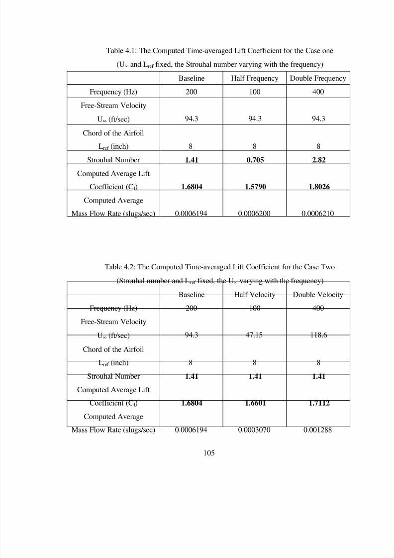
7/29/2019 Circulation Control Wing
http://slidepdf.com/reader/full/circulation-control-wing 125/192
105
Table 4.1: The Computed Time-averaged Lift Coefficient for the Case one
(U∞ and Lref fixed, the Strouhal number varying with the frequency)
Baseline Half Frequency Double Frequency
Frequency (Hz) 200 100 400
Free-Stream Velocity
U∞ (ft/sec) 94.3 94.3 94.3
Chord of the Airfoil
Lref (inch) 8 8 8
Strouhal Number 1.41 0.705 2.82
Computed Average Lift
Coefficient (Cl) 1.6804 1.5790 1.8026
Computed Average
Mass Flow Rate (slugs/sec) 0.0006194 0.0006200 0.0006210
Table 4.2: The Computed Time-averaged Lift Coefficient for the Case Two
(Strouhal number and Lref fixed, the U∞ varying with the frequency)
Baseline Half Velocity Double Velocity
Frequency (Hz) 200 100 400
Free-Stream Velocity
U∞ (ft/sec) 94.3 47.15 118.6
Chord of the Airfoil
Lref (inch) 8 8 8
Strouhal Number 1.41 1.41 1.41
Computed Average Lift
Coefficient (Cl) 1.6804 1.6601 1.7112
Computed Average
Mass Flow Rate (slugs/sec) 0.0006194 0.0003070 0.001288

7/29/2019 Circulation Control Wing
http://slidepdf.com/reader/full/circulation-control-wing 126/192
106
Table 4.3: The Computed Time-averaged Lift Coefficient for the Case Three
(Strouhal number and U∞ fixed, the Lref varying with the frequency)
Baseline Double Chord Half Chord
Frequency (Hz) 200 100 400
Free-Stream Velocity
U∞ (ft/sec) 94.3 94.3 94.3
Chord of the Airfoil
Lref (inch) 8 16 4
Strouhal Number 1.41 1.41 1.41
Computed Average Lift
Coefficient (Cl) 1.6804 1.7016 1.6743
Computed Average
Mass Flow Rate (slugs/sec) 0.0006194 0.001240 0.0003100

7/29/2019 Circulation Control Wing
http://slidepdf.com/reader/full/circulation-control-wing 127/192
107
0
0.01
0.02
0.03
0.04
0.05
0.06
0.07
0.08
0.09
0.21 0.212 0.214 0.216 0.218 0.22Real Time (sec)
M o m e n t u m C
o e f f i c i e n t , C
Sin Form Wave Pulsed Jets
Steady Jets
DT = 0.0025
Figure 4.1: The Time History of the Momentum Coefficient
(Sinusoidal Wave, Frequency = 400 Hz, Cµ,0 = 0.04)
0
0.5
1
1.5
2
2.5
0.21 0.212 0.214 0.216 0.218 0.22Real Time
L i f t C o e f f i c i e n t , C l
Sin Form Wave Pulsed Jets
Steady Jets
Figure 4.2: The Time History of the Lift Coefficient
(Sinusoidal Wave, Frequency = 400 Hz, Cµ,0 = 0.04)

7/29/2019 Circulation Control Wing
http://slidepdf.com/reader/full/circulation-control-wing 128/192
108
0
0.0002
0.0004
0.0006
0.0008
0.001
0.0012
0.0014
0.21 0.212 0.214 0.216 0.218 0.22
Real Time
M a s s F l o w
R a t e
Sin Form Wave Pulsed Jets
Steady Jets
Figure 4.3: The Time History of the Mass Flow Rate
(Sinusoidal Wave, Frequency = 400 Hz, Cµ,0 = 0.04)
0
0.4
0.8
1.2
1.6
2
0 20 40 60 80 100 120 140 160 180 200 220 240 260 280 300 320 340 360 380 400
Frequency (Hz)
L i f t C o e f f i c i e n t , C l
Steady Jet, Cmu=0.04
Sinusoidal Pulsed Jet, Ave. Cmu=0.04
Square Wave Pulsed Jet, Ave. Cmu=0.04
Figure 4.4: Time-averaged Lift Coefficient vs. Frequency

7/29/2019 Circulation Control Wing
http://slidepdf.com/reader/full/circulation-control-wing 129/192
109
0
0.0002
0.0004
0.0006
0.0008
0.001
0 20 40 60 80 100 120 140 160 180 200 220 240 260 280 300 320 340 360 380 400
Frequency (Hz)
M a s s F l o w
R a t e ( s l u g / s e
c )
Steady Jet, Cmu=0.04
Sinusoidal Form Pulsed Jet, Ave. Cmu=0.04
Square Wave Form Pulsed Jet, Ave. Cmu=0.04
Figure 4.5: Time-averaged Mass Flow Rate vs. Frequency
0
0.01
0.02
0.03
0.04
0.05
0.06
0.07
0.08
0.09
0.44 0.45 0.46 0.47 0.48 0.49Real Time
M o m e n t u m C
o e f f i c i e n t , C
Square Wave Pulsed Jet
Steady JetDT = 0.025 sec
Figure 4.6: The Time History of the Momentum Coefficient
(Square Wave Form, Frequency = 40 Hz, Cµ,0 = 0.04)

7/29/2019 Circulation Control Wing
http://slidepdf.com/reader/full/circulation-control-wing 130/192
110
0
0.5
1
1.5
2
2.5
0.44 0.45 0.46 0.47 0.48 0.49
Real Time
L i f t C o e f f i c i e n t , C l
Square Wave Pulsed Jet
Steady Jet
Figure 4.7: The Time History of the Lift Coefficient
(Square Wave Form, Frequency = 40 Hz, Cµ,0 = 0.04)
0
0.0002
0.0004
0.0006
0.0008
0.001
0.0012
0.0014
0.44 0.445 0.45 0.455 0.46 0.465 0.47 0.475 0.48 0.485 0.49
Real Time
M a s s F l o w
R a t e
Square Wave Pulsed Jet
Steady Jet
Figure 4.8: The Time History of the Mass Flow Rate
(Square Wave Form, Frequency = 40 Hz, Cµ,0 = 0.04)

7/29/2019 Circulation Control Wing
http://slidepdf.com/reader/full/circulation-control-wing 131/192
111
0
0.5
1
1.5
2
2.5
3
0 0.02 0.04 0.06 0.08 0.1 0.12 0.14
Time-Averaged Momentum Coefficient, C 0
C l
Steady Jet
Pulsed Jet , f = 40Hz
Pulsed Jet, f = 120 Hz
Pulsed Jet, f = 400 Hz
A
B
C
D
Figure 4.9: The Incremental Lift Coefficient vs. Time-averaged Momentum Coefficient
0
0.5
1
1.5
2
2.5
3
0 0.0002 0.0004 0.0006 0.0008 0.001 0.0012 0.0014 0.0016
Time Averaged Mass Flow Rate (slug/sec)
C l
Steady Jet
Pulsed Jet , f = 40Hz
Pulsed Jet, f = 120 Hz
Pulsed Jet, f = 400 Hz
A
B
C
D
Figure 4.10: The Incremental Lift Coefficient vs. Time-averaged Mass Flow Rate

7/29/2019 Circulation Control Wing
http://slidepdf.com/reader/full/circulation-control-wing 132/192
112
0
0.0002
0.0004
0.0006
0.0008
0.001
0.0012
0.0014
0.0016
0.0018
0.002
0 0.02 0.04 0.06 0.08 0.1 0.12 0.14
Time-Averaged Momentum Coefficient, C 0
T i m e A v e r a g e d M a s s F l o w
R a t e
( s l u g / s e c ) Steady Jet
Pulsed Jet , f = 40Hz
Pulsed Jet, f = 120 Hz
Pulsed Jet, f = 400 Hz
Figure 4.11: Time-averaged Mass Flow Rate vs. Time-averaged Momentum Coefficient
0
5
10
15
20
25
0 0.02 0.04 0.06 0.08 0.1 0.12 0.14
Time-Averaged Momentum Coefficient, C 0
E f f i c i e n c y ,
C l / ( C d + C
)
Steady Jet
Pulsed Jet , f = 40Hz
Pulsed Jet, f = 120 Hz
Pulsed Jet, f = 400 Hz
Figure 4.12: The Efficiency vs. Time-averaged Momentum Coefficient

7/29/2019 Circulation Control Wing
http://slidepdf.com/reader/full/circulation-control-wing 133/192
113
0
5
10
15
20
25
0 0.0002 0.0004 0.0006 0.0008 0.001 0.0012 0.0014 0.0016
Time Averaged Mass Flow Rate (slug/sec)
E f f i c i e n c y ,
C l / ( C d + C )
Steady Jet
Pulsed Jet , f = 40Hz
Pulsed Jet, f = 120 Hz
Pulsed Jet, f = 400 Hz
Figure 4.13: The Efficiency vs. Time-averaged Mass Flow Rate
0
0.4
0.8
1.2
1.6
2
0 20 40 60 80 100 120 140 160 180 200 220 240 260 280 300 320 340 360 380 400
Frequency (Hz)
L i f t C o e f f i c i e n t , C l
Steady Jet, Cmu=0.04
Pulsed Jet, Ave. Cmu=0.04
Figure 4.14: Time-averaged Lift Coefficient vs. Pulsed Jet Frequency (Ave. Cµ,0 = 0.04)

7/29/2019 Circulation Control Wing
http://slidepdf.com/reader/full/circulation-control-wing 134/192
114
0
2
4
6
8
10
12
14
16
18
20
0 20 40 60 80 100 120 140 160 180 200 220 240 260 280 300 320 340 360 380 400
Frequency (Hz)
E f f i c i e n c y ,
L / D
Steady Jet, Cmu=0.04
Pulsed Jet, Ave. Cmu=0.04
Figure 4.15: The Efficiency vs. Pulsed Jet Frequency (Ave. Cµ,0 = 0.04)
0
0.5
1
1.5
2
2.5
0.455 0.46 0.465 0.47 0.475 0.48 0.485 0.49 0.495
Real Time (sec)
L i f t C o e f f i c i e n t , C l
DT-cycle = 0.02501 sec
DT-down = 0.00335 sec
DT-up = 0.00137 sec
Figure 4.16: Time History of the Lift Coefficient for a 40 Hz Pulsed Jet

7/29/2019 Circulation Control Wing
http://slidepdf.com/reader/full/circulation-control-wing 135/192
115
0
0.5
1
1.5
2
2.5
0.21 0.212 0.214 0.216 0.218 0.22
Real Time (sec)
L i f t C o e f f i c i e n t , C l
DT-cycle = 0.00501 sec
DT-down = 0.00248 secDT-up
= 0.00113
Figure 4.17: Time History of the Lift Coefficient for a 200 Hz Pulsed Jet
1.2
1.4
1.6
1.8
2
50 100 150 200 250 300 350 400 450
Frequency
L i f t C o e f f i c i e n t , C
l
Case 1
Case 2
Case 3
Figure 4.18: Time-averaged Lift Coefficient vs. Frequency
(Case 1. Strouhal number was not fixed; U∞ and Lref were fixed)
(Case 2. Strouhal number and Lref were fixed; U∞ was not fixed)
(Case 3. Strouhal number and U∞ were fixed; Lref was not fixed)

7/29/2019 Circulation Control Wing
http://slidepdf.com/reader/full/circulation-control-wing 136/192
116
0
0.4
0.8
1.2
1.6
2
0 20 40 60 80 100 120 140 160 180 200 220 240 260 280 300 320 340 360 380 400
Frequency (Hz)
L i f t C o e f f i c i e n t , C l
Pulsed Jet, Ave. Cmu=0.04
Steady Jet, Cmu=0.04
0
Stouhal Number ( f * Chord / Vinf)
2.8281.414
Figure 4.19: Time-averaged Lift Coefficient vs. Frequency & Strouhal Number

7/29/2019 Circulation Control Wing
http://slidepdf.com/reader/full/circulation-control-wing 137/192
117
CHAPTER V
THREE DIMENSION CIRCULATION CONTROL WING
SIMULATIONS
The previous two chapters dealt with the use of Circulation Control for enhancing
the lift characteristics of 2-D airfoil configurations. It was demonstrated that both steady
and unsteady (pulsed) jets are effective in achieving high values of lift without resort to
the use of complex multi-element configurations.
Circulation Control has a number of other uses. It may be used to modify the
spanwise lift distribution of wing sections, effectively altering the span loading of lift
forces. Since the trailing vortex structures are directly affected by, and related to the
bound circulation, one can modify the strength (or spatial distribution) of trailing vortex
structures, including the strong vortex that forms at the wing tips.
This chapter addresses the uses and benefits of 3-D Circulation Control. Two
cases have been studied. The first is a streamwise tangential blowing on a wing-flap
configuration. The second is a spanwise tangential blowing over a rectangular wing with
a rounded wing tip. Some interesting results have been obtained for both cases,
demonstrating that there are many potential practical applications for the Circulation
Control technology, beyond high lift applications.

7/29/2019 Circulation Control Wing
http://slidepdf.com/reader/full/circulation-control-wing 138/192
118
5.1 Tangential Blowing on a Wing-flap Configuration
As mentioned in Chapter I, the flap edge vortex is always a strong source of the
airframe noise, especially when high lift devices are fully deployed during take-off or
landing. According to Prandtl’s classic lifting-line theory [21], a trailing vortex will be
generated whenever there is a change in the bound circulation over the wing. For a wing-
flap configuration, the lift and hence the bound circulation is much higher over the flap
than on the main wing. Thus the circulation will not be continuous at the interface
between the wing and the flap, and a very strong vortex will be generated here. These
vortices have been seen in many experiments and flight tests. For example, the
experimental [109] and computational [110] studies indicated that a very strong vortex
was generated at the flap-edge due to the sudden increase in the lift. This vortex, due to
its interaction with the flap gap, will generate a strong noise, commonly labeled as “flap-
edge noise”.
A number of approaches have been proposed to eliminate this noise source.
Vortex fences and serrated flap edges have been proposed and tested. These devices add
to the weight and cost of manufacturing of the wing. Because these are passive devices,
they can be at best optimized for a single operating condition (e.g. a specified flap angle,
flow angle of attack, and free-stream velocity), and can not be expected to work for all
conditions.

7/29/2019 Circulation Control Wing
http://slidepdf.com/reader/full/circulation-control-wing 139/192
119
C
This region is modeled as
shown in next figure
2-D BC
Symmetry BC
Small blowing to suppress vortex
shedding
15 C 5 C 5 C
C
This region is modeled as
shown in next figure
2-D BC
Symmetry BC
Small blowing to suppress vortex
shedding
15 C 5 C 5 C
Figure 5.1: The Wing-flap Tangential Blowing Configuration
The purpose of present research is to determine if the Circulation Control
technology may be used to modify the lift distribution along the span, thereby weakening
or eliminating the flap-edge vortex. Figure 5.1 shows a sketch of this concept – a wing-
flap configuration with tangential blowing over the main wing. Only the left half of this
wing-flap configuration has been simulated, and the flow has been assumed symmetric.
In this region, the wing section within the first five chord-length from the central
boundary has a 30-degree flap, and there is a weak jet blowing (Cµ ≅ 0.01) over the flap
to suppress the vortex shedding. The other part of the wing has no flap, but a scheduled
CC blowing is put in this section of the wing to generate high lift that is comparable with
the lift generated by the 30-degree flap.
Figure 5.2 shows details of the grid around this configuration. There are two
regions that are very important in these simulations. Region A is the interface

7/29/2019 Circulation Control Wing
http://slidepdf.com/reader/full/circulation-control-wing 140/192
120
between the blowing section of the main wing and the unblown section of the main wing,
and region B is the interface between the blowing section of the main wing and the wing-
flap section.
Three cases have been studied. In the first case, there is no blowing on the main
wing, so it is just a regular wing-flap configuration. In the second case, there is a constant
blowing, which means the Cµ is constant along the span, over some sections of the main
wing (from 15C to 20C). Finally, a gradual blowing case has been studied, where the C µ
is gradually increased along the span over some sections of the main wing (from 10C to
20C). Figure 5.3 shows the lift coefficient distribution along the span of this wing-flap
configuration for these three cases. When there is no blowing, a steep jump in lift
coefficient is found at the interface between the main wing and the flap. It is expected
because the sectional lift generated in the vicinity of the 30-degree flap is much higher
than the main wing. In the second case, when a constant blowing is put over a section of
the main wing, the lift at these stations will be greatly increased due to the Coanda effect.
Thus in Region B, the difference of lift between the blowing section of the main wing
and the flap will be reduced, but a jump in the lift is still found at the interface between
the blowing section of the main wing and the unblown section. In the third case involving
the gradually blowing, it is seen that the lift is smoothly increased along the span, from
0.25 to 1.4 over the flap without a sudden change. This is due to the gradual increase in
the blowing momentum coefficient, Cµ.
According to the lift distribution and the Prandtl’s lift ling theory, case 1 and 2
should generate strong vortices in Region B and A, respectively, while in case 3, there is

7/29/2019 Circulation Control Wing
http://slidepdf.com/reader/full/circulation-control-wing 141/192
121
a weakening or a total elimination of the flap-edge vortex. This has been observed in the
vorticity contours shown in Figures 5.4, 5.5 and 5.6. It should be noted that the
disturbance along the boundary of the flap-edge is due to the grid discontinuity along the
interface between the main wing and the flap, which is not a vortex.
In summary, the preliminary conclusions for the 3-D tangential streamwise
blowing over the wing-flap configuration are: 1) the flap-edge vortex is generated by the
suddenly increase in the lift along the flap-edge interface; 2) CC blowing with a constant
momentum coefficient can not eliminate the flap-edge vortex, but can weaken and move
the location of this vortex from the flap-edge towards the main wing; 3) a gradually
varying CC blowing can totally eliminate the vortex. It should be noted that this is just a
preliminary simulation, and that the model used here is very simple. To fully understand
the effect of the CC blowing on the flap-edge vortex, more detailed simulations are
recommended.
5.2 Spanwise Blowing over a Rounded Wing-tip
The vortex over the wing tip region is also a strong noise source. In rotor wing
applications, this vortex can interact with other blades, giving rise to blade vortex
interaction (BVI) noise. Tip vortex is generated by the pressure differences between the
upper and lower surface of the lift wing. Since in general, the pressure at the lower
surface is much higher than that at the upper surface, the vorticity of the fluid particles
within the boundary layer at the lower surface will flow around the wing tip, roll-up, and

7/29/2019 Circulation Control Wing
http://slidepdf.com/reader/full/circulation-control-wing 142/192
122
form a tip vortex. The tip vortex formation may be drastically altered by generating a
flow in a direction opposite to that of the boundary layer. To investigate the feasibility of
this concept, a wing-tip configuration has been studied on the effects of tangential
spanwise blowing on the flow field around the wing-tip region.
Figure 5.7 below shows a sketch of this concept for a rounded wing tip. The wing
is a simple rectangular wing with NACA 0012 airfoil sections, but the wing tip is round.
The angle of attack was 8 degrees, giving rise to sufficient lift and a strong tip vortex.
The jet slot is located above the rounded wing tip edge, and the jet is coming in the
spanwise direction. Figures 5.8 through 5.11 show the configuration and the body fitted
grid in the vicinity of the rounded wing tip and the jet slot.
Figure 5.7: The Wing Tip Configuration
Three cases have been studied. In the first case, there is no blowing, simulating a
rectangular wing with a rounded wing tip. In the second case, there is a small amount of
blowing with Cµ = 0.04. In the third case, there is a stronger blowing with Cµ = 0.18.
Figures 5.12, 5.13 and 5.14 show the vorticity contours around the wing tip region at
three different streamwise locations, which are x/c = 0.81, 1.0 and 1.50, respectively.
From those figures, it is seen that there is a strong tip vortex if there is no blowing, which

7/29/2019 Circulation Control Wing
http://slidepdf.com/reader/full/circulation-control-wing 143/192
123
is expected. If there is a small amount of blowing over the wing tip in the opposite
direction, the tip vortex will be pushed away from the wing tip, but the vortex could not
be eliminated. Even when the blowing is increased, the tip vortex is just pushed down
and far away from the wing. Another weaker vortex with an opposite rotation direction
has been generated. Figure 5.15 shows the velocity flow field around the wing tip region
at x/c = 0.81. It shows the same qualitative behavior as the vorticity contour.
Figures 5.16 and 5.17 show the lift and drag coefficients distribution along span
for this wing tip configuration. It is seen that the tangential blowing over the wing tip can
also increase the lift around whole wing, especially when there is a strong CC blowing.
The calculated overall lift coefficient and drag coefficient for the whole wing are tabled
as follows:
Table 5.1: The Total Lift Coefficient and Drag Coefficient for the Wing Tip
Configuration
Total LiftCoefficient
CL
Total DragCoefficient
CD
Computed Drag from theInviscid Relation
CD,C = (CL)2 /(πÆe)
Noblowing Case 0.4850 0.02997 0.02997
Less Blowing,
Cm = 0.04
0.5215 0.03078 0.03465
More Blowing,
Cm = 0.18
0.6064 0.04342 0.04685
where Æ is the aspect-ratio of the wing, which is equal to 4 for this configuration, and the
e is the efficiency of the lift distribution, which is set at 0.6246 from the noblowing case

7/29/2019 Circulation Control Wing
http://slidepdf.com/reader/full/circulation-control-wing 144/192
124
calculation. It is seen that the total drag of the wing has been reduced by about 10% by
CC blowing, when the drag has been corrected for the increase in C L.
The preliminary conclusions for the 3-D spanwise blowing over a rounded wing
tip configuration is that the jet blowing around the rounded wing tip can modify and
change the location of the tip vortex. It can not totally cancel or eliminate the tip vortex,
but can change or increase the vertical clearance between the wing and the vortex. Since
the blade vortex interaction of rotors is strongly influenced by the clearance between the
following blades and the tip vortex, this approach does have the potential of reducing
BVI noise. It can also slightly reduce the drag of the whole wing tip configuration by
pushing the tip vortex away from the wing, and increasing the aspect-ratio.
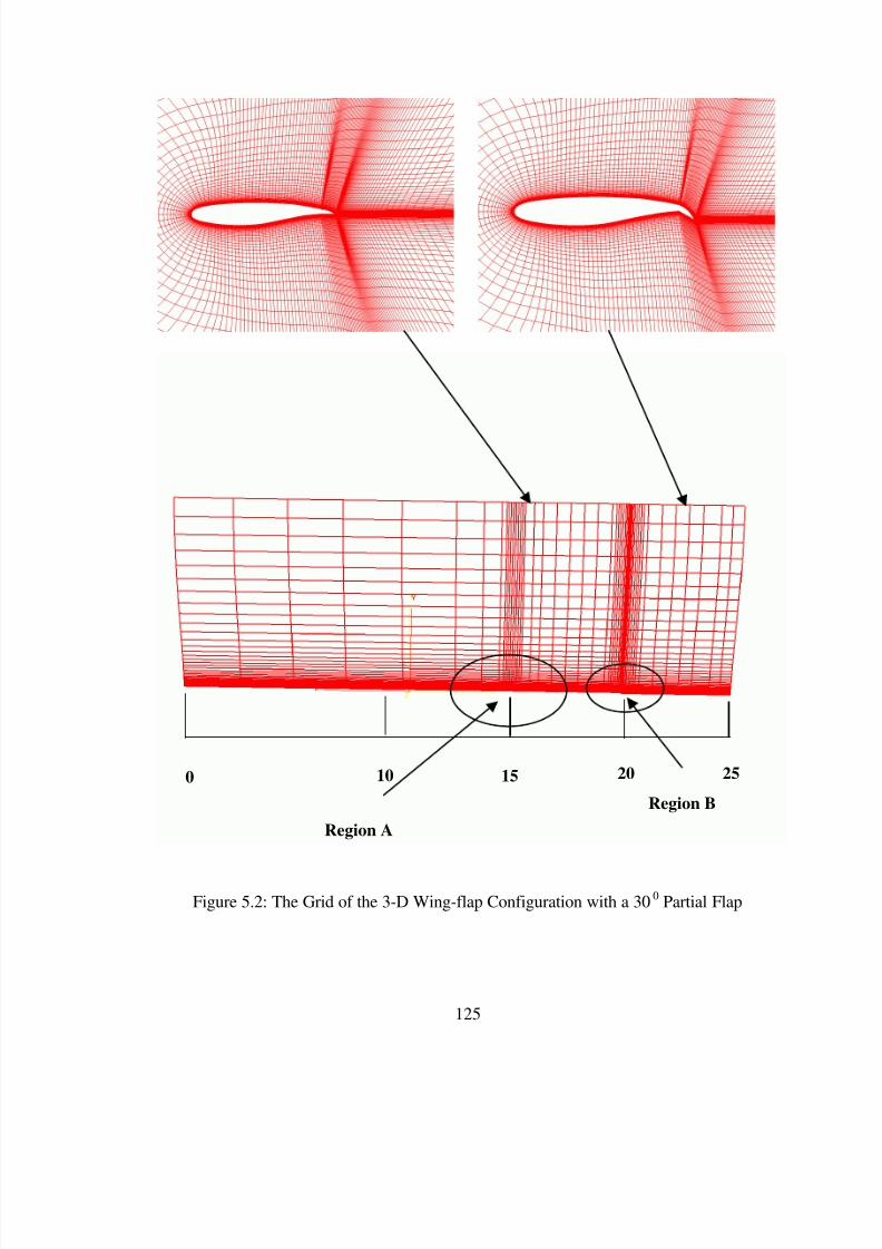
7/29/2019 Circulation Control Wing
http://slidepdf.com/reader/full/circulation-control-wing 145/192
125
Figure 5.2: The Grid of the 3-D Wing-flap Configuration with a 300 Partial Flap
Region A
Region B
0 20 251510

7/29/2019 Circulation Control Wing
http://slidepdf.com/reader/full/circulation-control-wing 146/192
126
0
0.2
0.4
0.6
0.8
1
1.2
1.4
1.6
0 5 10 15 20 25
Span, Y/C
L i f t C o e f f i c i e n t , C l
Noblowing on Main Wing
Constant Blowing on Main Wing
Gradual Blowing on Main Wing
Figure 5.3: The Lift Coefficient Distribution along Span for the Wing-flap Configuration

7/29/2019 Circulation Control Wing
http://slidepdf.com/reader/full/circulation-control-wing 147/192
127
Case 1: Noblowing Case
Figure 5.4: The Vorticity Contours for Noblowing Case
Flap Main Wing
Unblown SectionBlowing Section

7/29/2019 Circulation Control Wing
http://slidepdf.com/reader/full/circulation-control-wing 148/192
128
Case 2: Constant Blowing Case
Figure 5.5: The Vorticity Contours for Constant Blowing Case
Flap Main Wing
Unblown SectionBlowing Section

7/29/2019 Circulation Control Wing
http://slidepdf.com/reader/full/circulation-control-wing 149/192
129
Case 3: Gradual Blowing Case
Figure 5.6: The Vorticity Contours for Gradual Blowing Case
Flap Main Wing
Unblown SectionBlowing Section

7/29/2019 Circulation Control Wing
http://slidepdf.com/reader/full/circulation-control-wing 150/192
130
Figure 5.8: The H-Grid for the Wing Tip Configuration (Side View at Spanwise Station)
Figure 5.9: The O-Grid around the Rounded Wing Tip (Front View)

7/29/2019 Circulation Control Wing
http://slidepdf.com/reader/full/circulation-control-wing 151/192
131
Figure 5.10: The Surface Grid for the Rounded Wing Tip
Figure 5.11: The Detailed Grid Close to the Jet Slot

7/29/2019 Circulation Control Wing
http://slidepdf.com/reader/full/circulation-control-wing 152/192
132
Figure 5.12: The Vorticity Contours around the Wing Tip (x/C = 0.81)
No-Blowing
Case
Less Blowing
Case (C = 0.04)
More Blowing
Case (C = 0.18)

7/29/2019 Circulation Control Wing
http://slidepdf.com/reader/full/circulation-control-wing 153/192
133
Figure 5.13: The Vorticity Contours around the Wing Tip (x/C = 1.0)
No-Blowing
Case
Less Blowing
Case (C = 0.04)
More Blowing
Case (C = 0.18)

7/29/2019 Circulation Control Wing
http://slidepdf.com/reader/full/circulation-control-wing 154/192
134
Figure 5.14: The Vorticity Contours around the Wing Tip (x/C = 1.50)
No-Blowing
Case
Less Blowing
Case (C = 0.04)
More Blowing
Case (C = 0.18)

7/29/2019 Circulation Control Wing
http://slidepdf.com/reader/full/circulation-control-wing 155/192
135
Figure 5.15: The Velocity Vectors around the Wing Tip (x/C = 0.81)
No-Blowing
Case
Less Blowing
Case (C = 0.04)More Blowing
Case (C = 0.18)

7/29/2019 Circulation Control Wing
http://slidepdf.com/reader/full/circulation-control-wing 156/192
136
0
0.2
0.4
0.6
0.8
1
1.2
1.4
0 0.2 0.4 0.6 0.8 1 1.2
Span, Y/Ytip
C l
Noblowing
Blowing, Cmu = 0.04
Blowing, Cmu = 0.18
Figure 5.16: The Lift Coefficient Distribution along Span for Wing Tip Configuration
0
0.02
0.04
0.06
0.08
0.1
0.12
0.14
0.16
0.18
0.2
0 0.2 0.4 0.6 0.8 1 1.2
Span, Y/Ytip
C d
Noblowing
Blowing, Cmu = 0.04
Blowing, Cmu = 0.18
Figure 5.17: The Drag Coefficient Distribution along Span for Wing Tip Configuration
7/29/2019 Circulation Control Wing
http://slidepdf.com/reader/full/circulation-control-wing 157/192
137
CHAPTER VI
CONCLUSIONS AND RECOMMENDATIONS
In the present study, a three-dimensional unsteady Reynolds-average Navier-
Stokes analysis capable of modeling the Circulation Control Wings/Airfoils has been
developed. The method uses a semi-implicit finite difference scheme to solve the
governing equations on a body-fitted grid. A zero-equation Baldwin-Lomax and a one-
equation Spalart-Allmaras turbulence model have been implemented in the solver to
account for the turbulence effects. Physically appropriate boundary conditions are used to
model the jet exhausts from the slot located over the CCW flap. The solver can be used
both in a 2-D mode to compute the CC airfoil performance and in a 3-D mode for
studying CC wings.
The configuration selected is an advanced hinge-flap CC airfoil developed by
Englar, which has been extensively tested by Georgia Tech Research Institute (GTRI).
Prior to this work, the numerical studies for this kind of CC airfoils have been very
limited.
Prior to its use, a code-validation study has been done for a rectangular wing with
NACA 0012 airfoil sections. Subsequently, two-dimensional steady blowing simulations
have been done and compared with experimental data. The influence of some parameters
such as the slot-height and free-steam velocity on the performance of the CC airfoil has

7/29/2019 Circulation Control Wing
http://slidepdf.com/reader/full/circulation-control-wing 158/192
138
also been studied. The CCW configuration has also been compared with the baseline
unblown configuration and a conventional high-lift system. The effects the 2-D pulsed jet
on the CC airfoil performance have also been investigated. The effects of the wave shape
and the frequency of the pulsed jet have been specifically studied.
Finally, some simulations have been done for two three-dimensional
configurations with the use of the Circulation Control technology. The first involves a
streamwise tangential blowing on a wing-flap configuration to eliminate the flap-edge
vortex. The second study deals with the use of a spanwise blowing on a rounded wing-tip
configuration to control the tip vortex.
In this chapter, the conclusions of this research are presented in Section 6.1. The
recommendations for the future work are given in Section 6.2.
6.1 Conclusions
The investigation in the present study leads to the following major conclusions:
1. Navier-Stokes simulations are necessary for the CC wings/airfoils studies due to
the complexity of the flow field and the strong viscous effects. The results
indicate that this approach is an efficient and accurate way of modeling CC
airfoils with steady and pulsed jets.
2. The Circulation Control Technology is a useful way of achieving very high lift at
even zero angle of attack. It can also eliminate the vortex shedding in the trailing
edge region, which is a potential noise source. The lift coefficient of the CC

7/29/2019 Circulation Control Wing
http://slidepdf.com/reader/full/circulation-control-wing 159/192
139
airfoil is also increased with the angle of the attack as the conventional sharp
trailing edge airfoil. However, the stall angle of the CC airfoil is decreased
quickly with the increase in the blowing momentum coefficient. This stall
phenomenon occurs in the leading edge region, and may be suppressed by leading
edge blowing. In practice, because high CL values are achievable at low angles of
attack, it may seldom be necessary to operate CC wings at high angles of attack.
However, because there is always a large nose down pitch moment for the CC
airfoil, leading edge blowing is generally used to reduce this pitch moment for the
large amount of blowing case even at zero angle of attack.
3. The jet momentum coefficient varies uniquely with the total pressure of the jet
plenum. The behavior of computed lift coefficient is similar whether the
momentum coefficient or total jet pressure is varied. In experimental studies, it
may be more convenient to vary the jet total pressure, thereby changing the
momentum coefficient.
4. When the momentum coefficient is fixed, the computed lift coefficient does not
vary with the free-stream velocity. However, at a fixed Cµ, Cl is influenced by the
jet slot height. A thin jet from a smaller slot is preferred since it requires much
less mass flow, and has the same efficiency in generating the required Cl values as
a thick jet. From a practical perspective, much higher plenum pressure may be
needed to generate thin jets for a given Cµ. This may increase the power
requirements of compressors that provide the high pressure air.

7/29/2019 Circulation Control Wing
http://slidepdf.com/reader/full/circulation-control-wing 160/192
140
5. The CC airfoil with trailing edge blowing can generate higher lift and avoid static
stall compared to a conventional Fowler flap airfoil. It also achieves higher
efficiencies (Cl /(Cd+Cµ)) without the moving parts associated with the high-lift
system.
6. Sinusoidal pulsed jet was found not to be very effective compared to the square
wave pulsed jet due to higher mass flow rates required. A square wave shape
pulsed jet configuration gives larger increments in lift over the baseline unblown
configuration, when compared to the steady jet with the same time-averaged mass
flow rate. Pulsed jet performance is improved at higher frequencies due to the fact
that the airfoil has not fully shed the bound circulation into the wake before a new
pulse cycle begins.
7. The non-dimensional frequency, Strouhal number, has a more dominant effect on
the performance of the pulsed jet than just the frequency. Thus, the same
performance of a pulsed jet could be obtained at lower frequencies for a larger
configuration or at smaller free-stream velocities provided the Strouhal number is
kept the same. Furthermore, at a Strouhal number of 2 or above, the ∆Cl due to
pulsed jets is nearly 90% of ∆Cl achieved with the steady jet, while the mass flow
rate required is only 70% of the steady jet. Of course, an optimal Strouhal number
may be dependent on other physical parameters such as slot height, flap angle and
flap chord, etc. Nevertheless, it is clear that Strouhal number, and not the
frequency, is the dominant parameter.

7/29/2019 Circulation Control Wing
http://slidepdf.com/reader/full/circulation-control-wing 161/192
141
8. From the preliminary studies about the three-dimensional CC wing
configurations, it is found that a gradual streamwise tangential CC blowing near
the flap-edge can weaken or totally eliminate the flap-edge vortex, a strong noise
source. Spanwise tangential blowing over a rounded wing tip can push the tip
vortex down away from the wing tip. Thus an effective control of the tip vortex
position is feasible with Circulation Control.
6.2 Recommendations
While a number of computational issues have been addressed in this work,
additional work remains to be done before CFD based analysis such as the present work
can be confidently used to design CCW system. Research in following areas is
recommended:
1. Turbulence models are very important for the CC wing study, especially in the
area where strong separation and vortex shedding are present. The Baldwin-
Lomax and the Spalart-Allmaras turbulence models did a satisfactory job of
modeling the flow when the flow is attached and when there was no separation,
especially for the advanced CC airfoil with a sharp trailing edge flap. However, to
accurately simulate the strong tip vortex, the vortex shedding of the unblown
configuration, and the traditional rounded trailing edge CC airfoil, a systematic
study of improved turbulence models is necessary. Furthermore, many of the
existing models were developed or calibrated using steady flow data. Further

7/29/2019 Circulation Control Wing
http://slidepdf.com/reader/full/circulation-control-wing 162/192
142
calibrations or adjustments of the constants in these models may be necessary for
modeling the pulsed jet and unsteady flow.
2. The pulsed jet is a very effective way of obtaining the same high lift as a steady
jet while requiring lower mass flow rates. However, the desired high frequencies
are hard to achieve in experiments, especially when the test configuration is small.
Methods of improving the pulsed jet performance at low frequencies will be very
useful. One possibility is to vary the total jet pressure periodically instead of the
momentum coefficient. A second possibility is to change the slot height
dynamically while keeping a constant jet total pressure to generate a square wave
pulsed jet. However, the computational grid needs to be dynamically modified
with the change of the slot height. The current solver could not deal with this grid,
but this method is highly recommended for the future research of the pulsed jet.
3. There are many potential applications of the Circulation Control technology for
practical three-dimensional configurations beyond what has been studied in this
work. Some applications include: (a) drag reduction of bluff bodies and vehicles
such as trucks and automobiles, (b) Modification to the leading edge and exhaust
flow around engine nacelles, (c) suppression of vortex shedding from automobile
antennae and mirrors. The potential of this concept is limitless and should be
further explored, just keeping in mind the effect and cost involved in having a
readily available air source with some pressure.
7/29/2019 Circulation Control Wing
http://slidepdf.com/reader/full/circulation-control-wing 163/192
143
4. This work has addressed only the aerodynamic benefits of Circulation Control
wings. Elimination of high lift devices with this simple yet powerful approach can
reduce high lift system noise. However, it must be remembered that the high
speed steady or pulsed jet itself can be a source of noise. Thus a combined
aerodynamic/aeroacoustic analysis from a system wide perspective is necessary.
A companion experimental work by Munro [9], also funded by NASA (our
sponsor), looks at the issue of CCW noise in a careful manner. The numerical
studies of the aeroacoustic characteristics of CCW airfoils are recommended.
In conclusion, a first principle-based approach for modeling the Circulation
Control wing/airfoils has been developed and validated. It is hoped that this work will
serve as a useful step for the further investigations in this exciting area.

7/29/2019 Circulation Control Wing
http://slidepdf.com/reader/full/circulation-control-wing 164/192
144
APPENDIX A
GENERALIZED TRANSFORMATION
The generalized transformation is used to transform the governing equation from
the physical domain (x, y, z, t) to the computational domain (ξ, η, ζ, τ). In general, the
coordinates (ξ, η, ζ) in computational domain are assumed to be uniform spacing, and
they are the functions of (x, y, z) as follows:
t
)t,z,y,x(
)t,z,y,x(
)t,z,y,x(
=τ
ζ=ζ
η=η
ξ=ξ
(A.1)
For the time derivatives, the ξt, ηt and ζt are given in terms of the grid velocity xτ,
yτ and zτ as:
z
z
y
y
x
x
zz
yy
xx
zz
yy
xx
t
t
t
∂
ς∂−
∂
ς∂−
∂
ς∂−=ς
∂η∂
−∂η∂
−∂η∂
−=η
∂ξ∂
−∂ξ∂
−∂
ξ∂−=ξ
τττ
τττ
τττ
(A.2)
and the xτ, yτ and zτ are the grid velocity, and equal to zero if there is no body or grid
moving.
7/29/2019 Circulation Control Wing
http://slidepdf.com/reader/full/circulation-control-wing 165/192
145
For the spatial derivatives, using the chain rule of the partial differentiation, the
partial derivatives for coordinates (x, y, z) become:
ς∂∂
∂ς∂
+η∂∂
∂η∂
+ξ∂
∂∂ξ∂
=∂∂
ς∂∂
∂ς∂
+η∂∂
∂η∂
+ξ∂
∂∂ξ∂
=∂∂
ς∂∂∂ς∂+η∂∂∂η∂+ξ∂∂∂ξ∂=∂∂
zzzz
yyyy
xxxx
(A.3)
In above equation, for simplicity, the following expressions will be used for the
derivatives:
ς∂∂
=η∂
∂=
ξ∂∂
=∂ς∂
=ς∂
ς∂=ς
∂ς∂
=ς
ς∂∂
=η∂
∂=
ξ∂∂
=∂η∂
=η∂η∂
=η∂η∂
=η
ς∂∂
=η∂
∂=
ξ∂∂
=∂ξ∂
=ξ∂ξ∂
=ξ∂ξ∂
=ξ
ςηξ
ςηξ
ςηξ
zz,
zz,
zzand
z,
y,
x
yy,
yy,
yyand
z,
y,
x
xx,
xx,
xxand
z,
y,
x
zyx
zyx
zyx
(A.4)
Then, the differential expressions by the partial difference can be written as:
dzdydxd
dzdydxd
dzdydxd
zyx
zyx
zyx
ς+ς+ς=ς
η+η+η=η
ξ+ξ+ξ=ξ
(A.5)

7/29/2019 Circulation Control Wing
http://slidepdf.com/reader/full/circulation-control-wing 166/192
146
Equation (A.5) could be written in a matrix form as:
ςςς
ηηηξξξ
=
ς
ηξ
dz
dy
dx
d
d
d
zyx
zyx
zyx
(A.6)
Similarly, the (dx, dy, dz) can be expressed by (dξ, dη, dζ) as the following
matrix form:
ςηξ
=
ςηξ
ςηξ
ςηξ
d
d
d
zzz
yyy
xxx
dz
dy
dx
(A.7)
Combining equation (A.6) and (A.7), the following equation can be obtained:
−−−−−−−−−
=
=
ςςςηηηξξξ
ηηξηξξηξηηξ
ξξςξςςξςξξς
ςςηςηηςηςςη
−
ςηξ
ςηξ
ςηξ
xyxzxzxzyzy
xyxzxzxzyzy
xyxzxzxzyzy
J
zzz
yyy
xxx1
zyx
zyx
zyx
(A.8)
Thus, the derivatives of (ξ, η, ζ) can be expressed as:
)yxyx(J
)zxzx(J)zyzy(J
)yxyx(J
)zxzx(J)zyzy(J
)yxyx(J
)zxzx(J)zyzy(J
z
yx
z
yx
z
yx
ξηηξ
ηξξηξηηξ
ςξξς
ξςςξςξξς
ηςςη
ςηηςηςςη
−=ς
−=ς−=ς
−=η
−=η−=η
−=ξ
−=ξ−=ξ
(A.9)

7/29/2019 Circulation Control Wing
http://slidepdf.com/reader/full/circulation-control-wing 167/192
147
where J is the Jacobian Matrix of the transformation, which is given as:
)zyzy(x)zyzy(x)zyzy(x[ / 1
zzz
yyy
xxx
/ 1J
zyx
zyx
zyx
ξηηξςξςςξηηςςηξ
ςηξ
ςηξ
ςηξ
−+−−−=
=
ςςς
ηηηξξξ
= (A.10)
ξξξ z,y,x etc could be obtained by the differencing method. For instance, using
the second-order central difference, ξξξ z,y,x etc are expressed as follows:
ς∆
−=
ς∂∂
=
η∆
−=
η∂
∂=
ξ∆−
=ξ∂
∂=
ς∆−
=ς∂
∂=
η∆−=
η∂∂=
ξ∆−
=ξ∂
∂=
ς∆−
=ς∂
∂=
η∆−
=η∂
∂=
ξ∆−
=ξ∂
∂=
−+ς
−+η
−+ξ
−+ς
−+η
−+ξ
−+ς
−+η
−+ξ
2
zzzz
2
zzzz
2
zzzz
2
yyyy
2yyyy
2
yyyy
2
xxxx
2
xxxx
2
xxxx
1k , j,i1k , j,i
k , j,i
k , j,i,
k ,1 j,ik ,1 j,i
k , j,i
k , j,i,
k , j,1ik , j,1i
k , j,i
k , j,i,
1k , j,i1k , j,i
k , j,i
k , j,i,
k ,1 j,ik ,1 j,i
k , j,i
k , j,i,
k , j,1ik , j,1i
k , j,i
k , j,i,
1k , j,i1k , j,i
k , j,i
k , j,i,
k ,1 j,ik ,1 j,i
k , j,i
k , j,i,
k , j,1ik , j,1i
k , j,i
k , j,i,
(A.11)

7/29/2019 Circulation Control Wing
http://slidepdf.com/reader/full/circulation-control-wing 168/192
148
As for the fourth-order central difference, the following expressions could be
obtained for ςηξ x,x,x :
ς∆
+−+−=
ς∂∂
=
η∆
+−+−=
η∂∂
=
ξ∆+−+−
=ξ∂∂
=
−−++ς
−−++η
−−++
ξ
12
xx8x8xxx
12
xx8x8xxx
12
xx8x8xx
x
2k , j,i1k , j,i1k , j,i2k , j,i
k , j,i
k , j,i,
k ,2 j,ik ,1 j,ik ,1 j,ik ,2 j,i
k , j,i
k , j,i,
k , j,2ik , j,1ik , j,1ik , j,2i
k , j,i
k , j,i,
(A.12)
The similar equations could be obtained for ςηξ y,y,y and ςηξ z,z,z with y and
z, respectively.
Note that in most practical applications, the grid in the computational domain is
assumed to be uniform, thus the grid spacing ∆ξ , ∆η, and ∆ζ are equal to one.

7/29/2019 Circulation Control Wing
http://slidepdf.com/reader/full/circulation-control-wing 169/192
149
REFERENCES
1. “Noise Standards: Aircraft Type and Airworthiness Certification,” Federal
Aviation Regulations Part 36, Federal Aviation Administration, November 1969.
2. “Policies and Procedures For Considering Environmental Impacts,” Federal
Aviation Administration Order 1050.1D, December 1986.
3. Goldin, D. S., et al., National Aeronautics and Space Administration Strategic
Plan, NPD 1000.1B, pp. 42-43, September 2000.
4. Huff, D., “Recent Progress in Engine Noise Reduction for Commercial Aircraft
Applications.” Seminar, School of Aerospace Engineering, Georgia Institute of
Technology, April 8, 2003.
5. Smith, M. J. T., Aircraft Noise, Cambridge University Press, 1989.
6. Crighton, D. G., “Aircraft Noise in Aeronautics of Flight Vehicles: Theory andPractice,” Vol. 1: Noise Sources, NASA PR 1258, pp. 391-447, 1991.
7. Sen, R., “A Study of Unsteady Fields Near Leading-edge Slats,” AIAA Paper 97-1696, 1997.
8. Davy, R. and Remy, H., “Airframe Noise Characteristics on a 1/11 Scale AirbusModel,” AIAA Paper 98-2335, June 1998.
9. Munro, S., Jet Noise of High Aspect-Ratio Rectangular Nozzles with Application
to Pneumatic High-Lift Devices, Ph.D Thesis, Georgia Institute of Technology,2002.
10. Englar, R. J., “Circulation Control Pneumatic Aerodynamics: Blown Force andMoment Augmentation and Modification; Past, Present & Future”, AIAA Paper
2000-2541, June 2000.
11. Englar, Robert J., Smith, Marilyn J., Kelley, Sean M. and Rover, Richard C. III.,
“Application of Circulation Control to Advanced Subsonic Transport Aircraft,
Part I: Airfoil Development,” Journal of Aircraft , Vol.31 No.5, pp. 1160-1168,Sep. 1994.

7/29/2019 Circulation Control Wing
http://slidepdf.com/reader/full/circulation-control-wing 170/192
150
12. Englar, Robert J., Smith, Marilyn J., Kelley, Sean M. and Rover, Richard C. III.,
“Application of Circulation Control to Advanced Subsonic Transport Aircraft,
Part II: Transport Application,” Journal of Aircraft , Vol.31, No.5, pp. 1169-1177,Sep. 1994.
13. Shrewsbury, G. D. and Sankar, L. N., “Dynamic Stall of an OscillatingCirculation Control Airfoil,” International Symposium on Nonsteady Fluid
Dynamics, oronto, Canada, June 4-7, 1990, Proceedings. New York, American
Society of Mechanical Engineers, pp. 15-22, 1990.
14. Shrewsbury, G. D. and Sankar, L. N., “Dynamic Stall of Circulation Control
Airfoils,” AIAA Paper 90-0573, January 1990.
15. Salikuddin, M., Brown, W. H. and Ahuja, K. K., “Noise From a Circulation
Control Wing with Upper Surface Blowing,” Journal of Aircraft , Vol.24, pp55-
64, Jan. 1987.
16. Munro, S., Ahuja, K., and Englar, R., “Noise Reduction Through Circulation
Control Technology,” AIAA Paper 2001-0666, Jan. 2001.
17. Munro, S. and Ahuja, K. K., “Aeroacoustics of a High Aspect-Ratio Jet,” AIAA
paper 2003-3323, 2003, presented at the 9th
AIAA/CEAS AeroacousticsConference and Exhibit, Hilton Head, South Carolina, 12-14 May 2003.
18. Munro, S. and Ahuja, K. K., “Fluid Dynamics of a High Aspect-Ratio Jet,”
AIAA paper 2003-3129, 2003, presented at the 9th
AIAA/CEAS AeroacousticsConference and Exhibit, Hilton Head, South Carolina, 12-14 May 2003.
19. Munro, S. and Ahuja, K. K., “Development of a Prediction Scheme for Noise of High-Aspect Ratio Jets,” AIAA paper 2003-3255, 2003, presented at the 9 th
AIAA/CEAS Aeroacoustics Conference and Exhibit, Hilton Head, South
Carolina, 12-14 May 2003.
20. Liu, Y., Sankar, L. N., Englar, R. J. and Ahuja, K. K., “Numerical Simulations of
the Steady and Unsteady Aerodynamic Characteristics of a Circulation ControlWing Airfoil,” AIAA paper 2001-0704, January 2001.
21. Anderson, J. D. Jr., Fundamentals of Aerodynamics, Second Edition, McGraw-
Hill, Inc. 1991.
22. Metral, A. R., “On the Phenomenon of Fluid Veins and their Application, the
Coanda Effect”, AF Translation, F-TS-786-RE, 1939.

7/29/2019 Circulation Control Wing
http://slidepdf.com/reader/full/circulation-control-wing 171/192
151
23. Levinsky, E. S. and Yeh, T. T., “Analytical and Experimental Investigation of
Circulation Control by Means of a Turbulent Coanda Jet,” NASA CR-2114,
September, 1972.
24. Wood, N. J., “Circulation Control Airfoils: Past, Present and Future,” AIAA
paper 85-0204.
25. Englar, R. J. and Huson, G. G., “Development of Advanced Circulation Control
Wing High Lift Airfoils,” AIAA paper 83-1847, presented at AIAA AppliedAerodynamics Conference, July 1983.
26. Nichols, J. H. Jr, Englar, R. J., Harris, M. J. and Huson, G. G., “ExperimentalDevelopment of an Advanced Circulation Control Wing System for Navy STOL
Aircraft,” AIAA paper 81-0151, presented at AIAA Aerospace Science Meeting,
January 1981.
27. Englar, R. J., Hemmerly, R. A., Moore, H., Seredinsky, V., Valckenaere, W. G.and Jackson, J. A., “Design of the Circulation Control Wing STOL Demonstrator
Aircraft,” AIAA paper 79-1842, August, 1979.
28. Pugliese, A. J. and Englar, R. J., “Flight Testing the Circulation Control Wing,”
AIAA paper 79-1791, August 1979.
29. Englar, R. J., “Low-speed Aerodynamic Characteristics of a Small Fixed-
Trailing-Edge Circulation Control Wing Configuration Fitted to a Supercritical
Airfoil,” David Taylor Naval Ship Research and Development Center,DTNSRDC Report ASED-81/08, March 1981.
30. Englar, R. J., Niebur, J. S. and Gregory, S. D., “Pneumatic lift and control surfacetechnology for high speed civil transports,” Journal of Aircraft , vol. 36, no.2,
pp.332-339, Mar.-Apr., 1999.
31. Wilkerson, J. B., Reader, K. R. and Linck, D. W., “The Application of
Circulation Control Aerodynamics to a Helicopter Rotor Model,” American
Helicopter Society Paper AHS-704, May 1973.
32. Wilkerson, J. B., Barnes, D. R. and Bill, R. A., “The Circulation Control Rotor
Flight Demonstrator Test Program,” American Helicopter Society Paper AHS-
7951, May 1979.
33. Williams, R. M., Leitner, R. T. and Rogers, E. O., “X-Wing: A New Concept in
Rotary VTOL,” Presented at AHS Symposium on Rotor Technology, August1976.

7/29/2019 Circulation Control Wing
http://slidepdf.com/reader/full/circulation-control-wing 172/192
152
34. Englar R. J., “Development of Pneumatic Aerodynamic Devices to Improve the
Performance, Economics, and Safety of Heavy Vehicles,” SAE Paper 2000-01-
2208, June 2000.
35. Cheeseman, I. C. and Seed, A. R., “The Application of Circulation Control by
Blowing to Helicopter Rotors,” Journal of the Royal Aeronautical Society, Vol.71, July 1966.
36. Kind, R. J., A Proposed Method of Circulation Control, Ph.D Thesis, CambridgeUniversity, England, 1967.
37. Williams, R. M. and Howe, H. J., “Two-Dimensional Subsonic Wind TunnelTests on a 20% thick, 5% Cambered Circulation Control Airfoil,” NSRDC TN
AL-176, Aug. 1970.
38. Englar, R. J., “Two-Dimensional Transonic Wind Tunnel Tests of Three 15-
Percent Thick Circulation Control Airfoils,” NSRDC Rept. ASED-182, Dec.1970.
39. Englar, R. J., “Circulation Control for High Lift and Drag Generation on STOL
Aircraft,” Journal of Aircraft , Vol. 12, No. 5, pp.457, May 1975.
40. Abramson, J., “Two Dimensional Subsonic Wind Tunnel Evaluation of a 20
percent Thick Circulation Control Airfoil,” DTNSRDC Report ASED-311, 1975.
41. Abramson, J. and Rogers, E. O., “High-Speed Characteristics of CirculationControl Airfoils,” AIAA paper 83-0265, 1983.
42. Englar, R. J. and Applegate, C. A., “Circulation Control – A Bibliography of DTNSRDC Research and Selected Outside References (January 1969 through
December 1983),” DTNSRDC Report 84-052, 1984.
43. Carpenter, P. W., Bridson, D. W. and Green, P. N., “Features of Discrete Tones
Generated by Jet Flow over Coanda Surfaces,” AIAA paper 86-1685, 1986.
44. Howe, M. S., “Noise Generated by a Coanda Wall Jet Circulation Control
Device,” Journal of Sound and Vibration, Vol. 249, No.4, pp. 679-700, Jan. 2002.
45. Dvorak, F. A. and Kind, R. J., “Analysis Method for Viscous Flow OverCirculation-Controlled Airfoils,” AIAA paper 78-157, January 1978.
46. Dvorak, F. A. and Choi, D. H., “Analysis of Circulation Controlled Airfoils inTransonic Flow,” Journal of Aircraft , Vol. 20, pp.331-337, April 1983.

7/29/2019 Circulation Control Wing
http://slidepdf.com/reader/full/circulation-control-wing 173/192
153
47. Berman, H. A., “A Navier-Stokes Investigation of a Circulation Control Airfoil,”
Presented at AIAA 23rd
Aerospace Sciences Meeting, Reno, NV, Jan. 1985,
AIAA paper 85-0300.
48. Baldwin, B. S., and Lomax, H., “Thin Layer Approximation and Algebraic
Model for Separated Turbulent Flows,” AIAA Paper 78-257, Jan. 1978.
49. Pulliam, T. H., Jespersen, D. C. and Barth, T. J., “Navier-Stokes Computations
for Circulation Control Airfoils,” AIAA paper 85-1587.
50. Viegas, J. R., Rubesin, M. W. and MacCormack R. W., “ Navier-Stokes
Calculations and Turbulence Modeling in the Trailing Edge Region of ACirculation Control Airfoil,” Proceedings of the Circulation Control Workshop,
pp.1-22, 1986.
51. Spaid, F. W. and Keener, E. R., “Boundary-layer and Wake Measurements on a
Swept, Circulation-control Wing,” Proceedings of the Circulation ControlWorkshop, pp. 239-266, 1986.
52. Shrewsbury, G. D., “Analysis of Circulation Control Airfoils using an Implicit
Navier-Stokes Solver,” AIAA paper 85-0171, January 1985.
53. Shrewsbury, G. D., “Numerical Evaluation of Circulation Control Airfoil
Performance Using Navier-Stokes Methods,” AIAA paper 86-0286, January
1986.
54. Shrewsbury, G. D., “Numerical Study of a Research Circulation Control Airfoil
Using Navier-Stokes Methods,” Journal of Aircraft , Vol. 26, No. 1, pp.29-34,
1989.
55. Bradshaw, P., “Effects of Streamline Curvature on Turbulent Flow (applied to
boundary layer conditions on wing sections and turbomachine blades),” AGARD-AG-169, 1973.
56. Shrewsbury, G. D., Dynamic Stall of Circulation Control Airfoils, Ph.D Thesis,Georgia Institute of Technology, 1990.
57. Williams, S. L. and Franke, M. E., “Navier-Stokes Methods to Predict
Circulation Control Airfoil Performance,” Journal of Aircraft , Vol. 29, No.2,pp.243-249, March-April 1992.
58. Linton, S. W., “Computation of the Poststall Behavior of a Circulation ControlledAirfoil,” Journal of Aircraft , Vol. 31, No. 6, pp. 1273-1280, Nov. – Dec. 1994.

7/29/2019 Circulation Control Wing
http://slidepdf.com/reader/full/circulation-control-wing 174/192
154
59. Liu, J., Sun, M., and L. Wu, “Unsteady Flow about a Circulation Control Airfoil”,Science in China (Series E), Vol. 39, No. 1, Feb. 1996.
60. Wang, C., and Sun, M., “Aerodynamic Properties of Circulation Control Airfoil
with Multi-slot Blowing”, Acta Aerodynamica Sinica, vol. 17, no. 4, pp.378-383,
1999.
61. Englar, R. J., Smith, M. J., Kelley, S. M. and Rober, R. C. III, “Development of
Circulation Control Technology for Application to Advanced Subsonic TransportAircraft,” AIAA paper 93-0644, presented at 31st Aerospace Sciences Meeting &
Exhibit, Reno, NV, January 1993.
62. Slomski, J. F., Gorski, J. J., Miller, R. W. and Marino, T. A., “Numerical
Simulation of Circulation Control Airfoils as Affected by Different Turbulence
Models,” AiAA paper 2002-0851, 2002.
63. Yang, Z. Y. and Voke, P. R., “Large-eddy Simulation of Boundary-layerSeparation and Transition at a Change of Surface Curvature,” Journal of Fluid
Mechanics, Vol. 439, pp. 305-333, 2001.
64. Li, J. and Liu, C., “Direct Numerical Simulation for Flow Separation Control
with Pulsed Jets,” 41st
Aerospace Sciences Meeting and Exhibit, Reno NV, 2003,AIAA paper 2003-0611.
65. Kwon, J. and Sankar, L.N., “Numerical Study of the Effects of Icing on Finite
Wing Aerodynamics,” AIAA Paper 90-0757.
66. Bangalore, A., Phaengsook, N. and Sankar, L. N., “Application of a Third Order
Upwind Scheme to Viscous Flow over Clean and Iced Wings,” AIAA Paper 94-0485.
67. Sankar, L. N. and Wake, B., “Solutions of the Navier-Stokes Equations for theFlow about a Rotor Blade,” In National Specialists' Meeting on Aerodynamics
and Aeroacoustics, Arlington, TX, Feb. 25-27, 1987.
68. Sankar, L. N., Ruo, S. Y., Wake, B. E. and Wu, J., “An Efficient Rrocedure for
the Numerical Solution of Three-dimensional Viscous Flows,” Computational
Fluid Dynamics Conference, 8th, Honolulu, HI, June 9-11, 1987, AIAA Paper 87-
1159.
69. Tannehill, J. C., Anderson, D. A., and Pletcher, R. H., Computational Fluid
Mechanics and Heat Transfer , Second edition, Taylor & Francis, Washington,1997.

7/29/2019 Circulation Control Wing
http://slidepdf.com/reader/full/circulation-control-wing 175/192
155
70. Schlichting, H., Boundary-Layer Theory, 7th ed., translated by J. Kestin,
McGraw-Hill, New York, 1979.
71. Vincenti, W. G., and Kruger, C. H., Introduction to Physical Gas Dynamics, John
Wiley, New York, 1965.
72. Stokes, G. G., “On the Theories of Internal Friction of Fluids in Motion,” Trans.
Cambridge Phil. Soc., Vol. 8, pp. 287-305, 1845.
73. Fourier, J., The Analytical Theory of Heat , 1822, trans. By A. Freeman, 1878;
reprinted by Dover, New York, 1955.
74. Chapman, S., and Cowling, T. G., The Mathematical Theory of Non-uniform
Gases, Cambridge University Press, Cambridge, 1939, 1952.
75. Douglas, J., “On the Numerical Integration of ut = uxx + uyy by Implicit
Methods,” Journal of Society of Industrial and Applied Mathematics, Vol. 3,No.1, March 1955.
76. Peaceman, D. W. and Rachford, H. H., “The Numerical Solution of Parabolic and
Elliptic Differential Equations,” Journal of Society of Industrial and Applied
Mathematics, Vol. 3., No.1, March 1955.
77. Briley, W. and McDonald, H., “Solution of Multi-Component Navier-Stokes
Equations by Generalized Implicit Method,” Journal of Computational Physics,
Vol.24, p. 372, 1977.
78. Wake, B. E., Solution Procedure for the Navier-Stokes Equations Applied to
Rotors, Ph.D Thesis, Georgia Institute of Technology, Atlanta, GA 1987.
79. Beam R. and Warming R. F., “An Implicit Finite Difference Algorithm for
Hyperbolic Systems in Conservation Law form”, Journal of Computational
Physics, Vol.22, Sep. 1976, pp.87-110.
80. Pulliam, T. H., and Chaussee, D. S., “A Diagonal Form of An ImplicitApproximation Factorization Algorithm,” Journal of Computational Physics, Vol.
39, pp. 347-363, 1981.
81. Rizk, Y. M. and Chausee, D. S., “Three-Dimensional Viscous-FlowComputations Using a Directionally Hybrid Implicit-Explicit Procedure,” AIAA
Paper 83-1910, 1983.

7/29/2019 Circulation Control Wing
http://slidepdf.com/reader/full/circulation-control-wing 176/192
156
82. Tannehill, J. C., Holst, W. L. and Rakish, J. V. “Numerical Computation of Two-
Dimensional Viscous Blunt Body Flows with an Impinging Shock,” AIAA
Journal, Vol. 14, No.2, pp.204, 1976.
83. Von Neumann, J. and Richtmyer, R. D. “A Method for the Numerical Calculation
of Hydrodynamic Shocks,” Journal of Applied Physics, Vol. 21, pp. 232, 1950.
84. Lax, P. D. and Wendoff, B., “ Systems of Conservation Laws,” Communications
in Pure and Applied Mathematics, Vol. 13, pp. 217, 1960.
85. Lapidus, L., “A Detached Shock Calculation by Second-Order Finite-
Differences,” Journal of Computational Physics, Vol. 2, pp. 154, 1967.
86. Lindmuth, I. And Killeen, J., “Alternating Direction Implicit Techniques for
Two-Dimensional Magnetohydrodynamics Calculations,” Journal of
Computational Physics, Vol. 13, pp. 372, 1977.
87. McDonald, H. and Briley, W., “Three-Dimensional Supersonic Flow of a
Viscous or Inviscid Gas,” Journal of Computational Physics, Vol. 19, pp. 150-157, 1975.
88. Steger, J. L., “Implicit Finite-Difference Simulation of Flow about Arbitrary Two-Dimensional Geometry,” AIAA Journal, Vol. 16, No. 7, 1978.
89. Kim, J., Moin, P., and Moser, R., “Turbulence Statistics in Fully Developed
Channel Flow at Low Reynolds Number,” Journal of Fluid Mechanics, Vol. 177,1987, pp. 133-166.
90. Pope, S. B., Turbulent Flows, Cambridge University Press, 2000.
91. Spalart, P. R., and Allmaras, S. R., “A One-Equation Turbulence Model for
Aerodynamic Flows,” AIAA Paper 92-0439, Jan. 1992.
92. Cebeci, T., “Calculation of Compressible Turbulent Boundary Layers with Heat
and Mass Transfer,” AIAA Paper 70-741, AIAA 3rd
Fluid and Plasma DynamicsConference, Los Angeles, CA, June 1970.
93. Michel, R., and Arnal, D., “Investigation of the Conditions for Tripping
Transition with Roughness Elements and their Influence on Boundary LayerDevelopment,” ESA Boundary Layer Control by Transition Fixing (ESA-TT-
909), pp.103-113, 1984.
94. Eppler, R., and Fasel, H., “Laminar-turbulent Transition,” Proceedings of the
Symposium, Stuttgart, West Germany, September 16-22, 1979.

7/29/2019 Circulation Control Wing
http://slidepdf.com/reader/full/circulation-control-wing 177/192
157
95. Bragg, M. B., and Spring, S. A., “An Experimental Study of the Flow Field about
an Airfoil with Glaze Ice,” Presented at the AIAA 25th
Aerospace Science
Meeting, Reno, Nevada, AIAA paper 87-0100, Jan 12-15, 1987.
96. Dancila, D. S. and Vasilescu, R., “Modeling of Piezoelectrically Modulated and
Vectored Blowing For a Wing Section,” AIAA paper 2003-0219, presented at41st AIAA Aerospace Sciences Meeting & Exhibit, Reno, NV, Jan. 6-9, 2003.
97. Bangalore, A. K., Sankar, L. N., and Tseng, W., “A Multi-zone Navier-StokesAnalysis of Dynamic Lift Enhancement Concepts,” AIAA, Aerospace Sciences
Meeting & Exhibit, 32nd, Reno, NV, Jan. 10-13, 1994, AIAA Paper 94-0164.
98. Bangalore, A. K., and Sankar, L. N., “Numerical Analysis of Aerodynamic
Performance of Rotors with Leading Edge Slats,” AIAA Applied Aerodynamics
Conference, 13th, San Diego, CA, June 19-22, 1995, AIAA Paper 95-1888.
99. Valarezo, W. O., Dominik, C. J., McGhee, R. J., and Goodman, W. L., “HighReynolds Number Configuration Development of a High-Lift Airfoil,” AGARD
Conference Proceedings 515, AGARD-CP-515, No.10, 1993.
100. Cock, K. de, “High-Lift System Analysis Method using Unstructured Meshes,”
AGARD Conference Proceedings 515, AGARD-CP-515, No.12, 1993.
101. Seifert, A., Darabi, A. and Wygnanski, I., “Delay of Airfoil Stall by Periodic
Excitation,” AIAA Journal of Aircraft , Vol. 33, No. 4, 1996.
102. Wygnanski, I, “Some New Observations Affecting the Control of Separation by
Periodic Excitation,” AIAA 2000-2314, FLUIDS 2000 Conference and Exhibit,
Denver, CO, 19-22 June, 2000.
103. Lorber, P.F., McCormick, D., Anderson, T., Wake, B.E., MacMartin, D., Pollack,
M., Corke, T., and Breuer, K., “Rotorcraft Retreating Blade-Stall Control,” AIAA2000-2475, FLUIDS 2000 Conference and Exhibit, Denver, CO, 19-22 June,
2000.
104. Wake, B. and Lurie, E. A., "Computational Evaluation of Directed Synthetic Jets
for Dynamic Stall Control,” AHS International Annual Forum, 57th, Washington,
DC, May 9-11, 2001, Proceedings (A02-12351 01-05), Alexandria, VA, AHS
International, 2001.
105. Hassan, A., and Janakiram, R. D., “Effects of Zero-Mass Synthetic Jets on the
Aerodynamics of the NACA 0012 Airfoil,” Journal of the American Helicopter
Society, Vol. 43, No. 4, October, 1998.
7/29/2019 Circulation Control Wing
http://slidepdf.com/reader/full/circulation-control-wing 178/192
158
106. Oyler, T.E., and W.E. Palmer, “Exploratory Investigation of Pulse Blowing for
Boundary Layer Control,” North American Rockwell Report NR72H-12, Jan.
1972.
107. Schatz, M., and Thiele, F., “Numerical Study of High-Lift Flow with Separation
Control by Periodic Excitation,” AIAA Paper 2001-0296, Jan. 2001.
108. Sun, M., and Hamdani, H., “Separation Control by Alternating Tangential
Blowing/Suction at Multiple Slots,” AIAA Paper 2001-0297, Jan. 2001.
109. Radeztsky, R. H., Singer, B. A. and Khorrami, M. R., “Detailed Measurements of
a Flap Side-edge Flow Field,” AIAA paper 98-0700, Jan. 1998.
110. Khorrami, M. R., Singer, B. A. and Radeztsky, R. H., “Reynolds Averaged
Navier-Stokes Computations of a Flap Sied-edge Flow Field,” AIAA paper 98-
0768, Jan. 1998.

7/29/2019 Circulation Control Wing
http://slidepdf.com/reader/full/circulation-control-wing 179/192
159
VITA
Yi Liu was born in Hunan province, China on June 1, 1973. He graduated from
Beijing University of Aeronautics & Astronautics, China, with a Bachelor of Science
(B.Sc) degree in Aerospace Engineering in July 1994. He worked as an aerospace
engineer in the Nanhua Jet Engine Research Institute from 1994 to 1995. Then he
continued his graduate study in the Department of Jet Propulsion of Beijing University of
Aeronautics & Astronautics, China, and earned a Master of Science (M.Sc) degree in
April 1998. In September 1998, he joined the Ph.D program in the School of Aerospace
Engineering at the Georgia Institute of Technology, Atlanta, Georgia. He is a student
member of the American Helicopter Society and the American Institute of Aeronautics
and Astronautics.

7/29/2019 Circulation Control Wing
http://slidepdf.com/reader/full/circulation-control-wing 180/192
160
1 “Noise Standards: Aircraft Type and Airworthiness Certification,” Federal Aviation
Regulations Part 36, Federal Aviation Administration, November 1969.
2 “Policies and Procedures For Considering Environmental Impacts,” Federal Aviation
Administration Order 1050.1D, December 1986.
3 Goldin, D. S., et al., National Aeronautics and Space Administration Strategic Plan,
NPD 1000.1B, pp. 42-43, September 2000.
4 Huff, D., “Recent Progress in Engine Noise Reduction for Commercial Aircraft
Applications.” Seminar, School of Aerospace Engineering, Georgia Tech, April 8,
2003.
5 Smith, M. J. T., “Aircraft Noise,” Cambridge University Press, 1989.
6 Crighton, D. G., “Aircraft Noise in Aeronautics of Flight Vehicles: Theory and
Practice,” Vol. 1: Noise Sources, NASA PR 1258, pp. 391-447, 1991.
7 Sen, R., “A Study of Unsteady Fields Near Leading-edge Slats,” AIAA 97-1696, 1997.
8 Davy, R. and Remy, H., “Airframe Noise Characteristics on a 1/11 Scale Airbus
Model,” AIAA Paper 98-2335, June 1998.
9 Munro, S., “Jet Noise of High Aspect-Ratio Rectangular Nozzles with Application to
Pneumatic High-Lift Devices,” Ph.D Thesis, Georgia Institute of Technology, 2002.
10 Englar, R. J., “Circulation Control Pneumatic Aerodynamics: Blown Force and
Moment Augmentation and Modification; Past, Present & Future”, AIAA Paper 2000-
2541, June 2000.

7/29/2019 Circulation Control Wing
http://slidepdf.com/reader/full/circulation-control-wing 181/192
161
11 Englar, Robert J., Smith, Marilyn J., Kelley, Sean M. and Rover, Richard C. III.,
“Application of Circulation Control to Advanced Subsonic Transport Aircraft, Part I:
Airfoil Development,” Journal of Aircraft, Vol.31 No.5, pp. 1160-1168, Sep. 1994.
12 Englar, Robert J., Smith, Marilyn J., Kelley, Sean M. and Rover, Richard C. III.,
“Application of Circulation Control to Advanced Subsonic Transport Aircraft, Part II:
Transport Application,” Journal of Aircraft, Vol.31, No.5, pp. 1169-1177, Sep. 1994.
13 Shrewsbury, G. D. and Sankar, L. N., “Dynamic stall of an oscillating circulation
control airfoil,” International Symposium on Nonsteady Fluid Dynamics, Toronto,
Canada, June 4-7, 1990, Proceedings. New York, American Society of Mechanical
Engineers, pp. 15-22, 1990.
14 Shrewsbury, G. D. and Sankar, L. N., “Dynamic Stall of Circulation Control Airfoils,”
AIAA Paper 90-0573, January 1990.
15 Salikuddin, M., Brown, W. H. and Ahuja, K. K., “Noise From a Circulation Control
Wing with Upper Surface Blowing,” Journal of Aircraft, Vol.24, pp55-64, Jan. 1987.
16 Munro, S., Ahuja, K., and Englar, R., “Noise Reduction Through Circulation Control
Technology,” AIAA Paper 2001-0666, Jan. 2001.
17 Munro, S. and Ahuja, K. K., “Aeroacoustics of a High Aspect-Ratio Jet,” AIAA paper
2003-3323, 2003, presented at the 9th AIAA/CEAS Aeroacoustics Conference and
Exhibit, Hilton Head, South Carolina, 12-14 May 2003.
18 Munro, S. and Ahuja, K. K., “Fluid Dynamics of a High Aspect-Ratio Jet,” AIAA
paper 2003-3129, 2003, presented at the 9th AIAA/CEAS Aeroacoustics Conference
and Exhibit, Hilton Head, South Carolina, 12-14 May 2003.

7/29/2019 Circulation Control Wing
http://slidepdf.com/reader/full/circulation-control-wing 182/192
162
19 Munro, S. and Ahuja, K. K., “Development of a Prediction Scheme for Noise of High-
Aspect Ratio Jets,” AIAA paper 2003-3255, 2003, presented at the 9 th AIAA/CEAS
Aeroacoustics Conference and Exhibit, Hilton Head, South Carolina, 12-14 May 2003.
20 Liu, Y., Sankar, L. N., Englar, R. J. and Ahuja, K. K., “Numerical Simulations of the
Steady and Unsteady Aerodynamic Characteristics of a Circulation Control Wing
Airfoil,” AIAA paper 2001-0704, January 2001.
21 Anderson, J. D. Jr., “Fundamentals of Aerodynamics”, Second Edition, McGraw-Hill,
Inc. 1991.
22 Metral, A. R., “On the Phenomenon of Fluid Veins and their Application, the Coanda
Effect”, AF Translation, F-TS-786-RE, 1939.
23 Levinsky, E. S. and Yeh, T. T., “Analytical and Experimental Investigation of
Circulation Control by Means of a Turbulent Coanda Jet,” NASA CR-2114,
September, 1972.
24 Wood, N. J., “Circulation Control Airfoils: Past, Present and Future,” AIAA paper 85-
0204.
25 Englar, R. J. and Huson, G. G., “Development of Advanced Circulation Control Wing
High Lift Airfoils,” AIAA paper 83-1847, presented at AIAA Applied Aerodynamics
Conference, July, 1983.
26 Nichols, J. H. Jr, Englar, R. J., Harris, M. J. and Huson, G. G., “Experimental
Development of an Advanced Circulation Control Wing System for Navy STOL
Aircraft,” AIAA paper 81-0151, presented at AIAA Aerospace Science Meeting,
January, 1981.

7/29/2019 Circulation Control Wing
http://slidepdf.com/reader/full/circulation-control-wing 183/192
163
27 Englar, R. J., Hemmerly, R. A., Moore, H., Seredinsky, V., Valckenaere, W. G. and
Jackson, J. A., “Design of the Circulation Control Wing STOL Demonstrator Aircraft,”
AIAA paper 79-1842, August, 1979.
28 Pugliese, A. J. and Englar, R. J., “Flight Testing the Circulation Control Wing,” AIAA
paper 79-1791, August, 1979.
29 Englar, R. J., “Low-speed Aerodynamic Characteristics of a Small Fixed-Trailing-
Edge Circulation Control Wing Configuration Fitted to a Supercritical Airfoil,” David
W. Taylor Naval Ship Research and Development Center, DTNSRDC Report ASED-
81/08, March, 1981.
30 Englar, R. J., Niebur, J. S. and Gregory, S. D., “Pneumatic lift and control surface
technology for high speed civil transports,” Journal of Aircraft, vol. 36, no.2, pp.332-
339, Mar.-Apr., 1999.
31 Wilkerson, J. B., Reader, K. R. and Linck, D. W., “The Application of Circulation
Control Aerodynamics to a Helicopter Rotor Model,” American Helicopter Society
Paper AHS-704, May, 1973.
32 Wilkerson, J. B., Barnes, D. R. and Bill, R. A., “The Circulation Control Rotor Flight
Demonstrator Test Program,” American Helicopter Society Paper AHS-7951, May,
1979.
33 Williams, R. N., Leitner, R. T. and Rogers, E. O., “X-Wing: A New Concept in
Rotary VTOL,” Presented at AHS Symposium on Rotor Technology, August, 1976.

7/29/2019 Circulation Control Wing
http://slidepdf.com/reader/full/circulation-control-wing 184/192
164
34 Englar R. J., “Development of Pneumatic Aerodynamic Devices to Improve the
Performance, Economics, and Safety of Heavy Vehicles,” SAE Paper 2000-01-2208,
June, 2000.
35 Cheeseman, I. C. and Seed, A. R., “The Application of Circulation Control by
Blowing to Helicopter Rotors,” Journal of the Royal Aeronautical Society, Vol. 71,
July, 1966.
36 Kind, R. J., “A Proposed Method of Circulation Control,” Ph.D Thesis, Cambridge
University, England.
37 Williams, R. M. and Howe, H. J., “Two-Dimensional Subsonic Wind Tunnel Tests on
a 20% thick, 5% Cambered Circulation Control Airfoil,” NSRDC TN AL-176, Aug.
1970.
38 Englar, R. J., “Two-Dimensional Transonic Wind Tunnel Tests of Three 15-Percent
Thick Circulation Control Airfoils,” NSRDC Rept. ASED-182, Dec. 1970.
39 Englar, R. J., “Circulation Control for High Lift and Drag Generation on STOL
Aircraft,” Journal of Aircraft, Vol. 12, No. 5, pp.457, May 1975.
40 Abramson, J., “Two Dimensional Subsonic Wind Tunnel Evaluation of a 20 percent
Thick Circulation Control Airfoil,” DTNSRDC Report ASED-311, 1975.
41 Abramson, J. and Rogers, E. O., “High-Speed Characteristics of Circulation Control
Airfoils,” AIAA paper 83-0265, 1983.
42 Englar, R. J. and Applegate, C. A., “Circulation Control – A Bibliography of
DTNSRDC Research and Selected Outside References (January 1969 through
December 1983),” DTNSRDC Report 84-052, 1984.

7/29/2019 Circulation Control Wing
http://slidepdf.com/reader/full/circulation-control-wing 185/192
165
43 Carpenter, P. W., Bridson, D. W. and Green, P. N., “Features of Discrete Tones
Generated by Jet Flow over Coanda Surfaces,” AIAA paper 86-1685, 1986.
44 Howe, M. S., “Noise Generated by a Coanda Wall Jet Circulation Control Device,”
Journal of Sound and Vibration, Vol. 249, No.4, pp. 679-700, Jan. 2002.
45 Dvorak, F. A. and Kind, R. J., “Analysis Method for Viscous Flow Over Circulation-
Controlled Airfoils,” Journal of Aircraft, Vol. 16, No. 1, January 1979.
46 Dvorak, F. A. and Choi, D. H., “Analysis of Circulation Controlled Airfoils in
Transonic Flow,” Journal of Aircraft, Vol. 20, April 1983.
47 Berman, H. A., “A Navier-Stokes Investigation of a Circulation Control Airfoil,”
AIAA paper 85-0300.
48 Baldwin, B. S., and Lomax, H., “Thin Layer Approximation and Algebraic Model for
Separated Turbulent Flows,” AIAA Paper 78-257, Jan. 1978.
49 Pulliam, T. H., Jespersen, D. C. and Barth, T. J., “Navier-Stokes Computations for
Circulation Control Airfoils,” AIAA paper 85-1587.
50 Viegas, J. R., Rubesin, M. W. and MacCormack R. W., “ Navier-Stokes Calculations
and Turbulence Modeling in the Trailing Edge Region of A Circulation Control
Airfoil,” NASA CP-2432.
51 Spaid, F. W. and Keener, E. R., “Boundary-layer and wake measurements on a swept,
circulation-control wing,” AIAA, Aerospace Sciences Meeting, 25th, Reno, NV, Jan.
12-15, 1987, AIAA Paper 87-0156.
52 Shrewsbury, G. D., “Analysis of Circulation Control Airfoils using an Implicit Navier-
Stokes Solver,” AIAA paper 85-0171, January 1985.

7/29/2019 Circulation Control Wing
http://slidepdf.com/reader/full/circulation-control-wing 186/192
166
53 Shrewsbury, G. D., “Numerical Evaluation of Circulation Control Airfoil Performance
Using Navier-Stokes Methods,” AIAA paper 86-0286, January 1986.
54 Shrewsbury, G. D., “Numerical Study of a Research Circulation Control Airfoil Using
Navier-Stokes Methods,” Journal of Aircraft, Vol. 26, No. 1, pp.29-34, 1989.
55 Bradshaw, P., “Effects of Streamline Curvature on Turbulent Flow (applied to
boundary layer conditions on wing sections and turbomachine blades),” AGARD-AG-
169, 1973.
56 Shrewsbury, G. D., “Dynamic Stall of Circulation Control Airfoils,” Ph.D Thesis,
Georgia Institute of Technology, 1990.
57 Williams, S. L. and Franker, M. E., “Navier-Stokes Methods to Predict Circulation
Control Airfoil Performance,” Journal of Aircraft, Vol. 29, No.2, pp.243-249, March-
April 1992.
58 Linton, S. W., “Computation of the Poststall Behavior of a Circulation Controlled
Airfoil,” Journal of Aircraft, Vol. 31, No. 6, pp. 1273-1280, Nov. – Dec. 1994.
59 Liu, J., Sun, M., and L. Wu, “Unsteady Flow about a Circulation Control Airfoil”,
Science in China (Series E), Vol. 39, No. 1, Feb. 1996.
60 Wang, C., and Sun, M., “Aerodynamic Properties of Circulation Control Airfoil with
Multi-slot Blowing”, Acta Aerodynamica Sinica, vol. 17, no. 4, pp.378-383, 1999.
61 Englar, R. J., Smith, M. J., Kelley, S. M. and Rober, R. C. III, “Development of
Circulation Control Technology for Application to Advanced Subsonic Transport
Aircraft,” AIAA paper 93-0644, presented at 31st Aerospace Sciences Meeting &
Exhibit, Reno, NV, January 1993.

7/29/2019 Circulation Control Wing
http://slidepdf.com/reader/full/circulation-control-wing 187/192
167
62 Slomski, J. F., Gorski, J. J., Miller, R. W. and Marino, T. A., “Numerical Simulation
of Circulation Control Airfoils as Affected by Different Turbulence Models,” AiAA
paper 2002-0851, 2002.
63 Yang, Z. Y. and Voke, P. R., “Large-eddy simulation of boundary-layer separation
and transition at a change of surface curvature,” Journal of Fluid Mechanics, Vol. 439,
pp. 305-333, 2001.
64 Li, J. and Liu, C., “Direct Numerical Simulation for Flow Separation Control with
Pulsed Jets,” 41
st
Aerospace Sciences Meeting and Exhibit, Reno NV, 2003, AIAA
paper 2003-0611.
65 Kwon, J. and Sankar, L.N., “Numerical Study of the Effects of Icing on Finite Wing
Aerodynamics,” AIAA Paper 90-0757.
66 Bangalore, A., Phaengsook, N. and Sankar, L. N., “Application of a Third Order
Upwind Scheme to Viscous Flow over Clean and Iced Wings,” AIAA Paper 94-0485.
67 Sankar, L. N. and Wake, B., “Solutions of the Navier-Stokes equations for the flow
about a rotor blade,” In National Specialists' Meeting on Aerodynamics and
Aeroacoustics, Arlington, TX, Feb. 25-27, 1987.
68 Sankar, L. N., Ruo, S. Y., Wake, B. E. and Wu, J., “An efficient procedure for the
numerical solution of three-dimensional viscous flows,” Computational Fluid
Dynamics Conference, 8th, Honolulu, HI, June 9-11, 1987, AIAA Paper 87-1159.
69 Tannehill, J. C., Anderson, D. A., and Pletcher, R. H., “Computational Fluid
Mechanics and Heat Transfer,” Second edition, Taylor & Francis, Washington, 1997.

7/29/2019 Circulation Control Wing
http://slidepdf.com/reader/full/circulation-control-wing 188/192
168
70 Schlichting, H., “Boundary-Layer Theory,” 7th
ed., translated by J. Kestin, McGraw-
Hill, New York, 1979.
71 Vincenti, W. G., and Kruger, C. H., “Introduction to Physical Gas Dynamics,” John
Wiley, New York, 1965.
72 Stokes, G. G., “On the Theories of Internal Friction of Fluids in Motion,” Trans.
Cambridge Phil. Soc., Vol. 8, pp. 287-305, 1845.
73 Fourier, J., “The Analytical Theory of Heat”, 1822, trans. By A. Freeman, 1878;
reprinted by Dover, New York, 1955.
74 Chapman, S., and Cowling, T. G., “The Mathematical Theory of Non-uniform Gases,”
Cambridge University Press, Cambridge, 1939, 1952.
75 Douglas, J., “On the Numerical Integration of ut = uxx + uyy by Implicit Methods,”
Journal of Society of Industrial and Applied Mathematics, Vol. 3, No.1, March 1955.
76 Peaceman, D. W. and Rachford, H. H., “The Numerical Solution of Parabolic and
Elliptic Differential Equations,” Journal of Society of Industrial and Applied
Mathematics, Vol. 3., No.1, March 1955.
77 Briley, W. and McDonald, H., “Solution of Multi-Component Navier-Stokes
Equations by Generalized Implicit Method,” Journal of Computational Physics, Vol.24,
p. 372, 1977
78 Wake, B. E., “Solution Procedure for the Navier-Stokes Equations Applied to Rotors,”
Ph.D Thesis, Georgia Institute of Technology, Atlanta, GA 1987.

7/29/2019 Circulation Control Wing
http://slidepdf.com/reader/full/circulation-control-wing 189/192
169
79 Beam R. and Warming R. F., “An Implicit Finite Difference Algorithm for Hyperbolic
Systems in Conservation Law form”, Journal of Computational Physics, Vol.22, Sep.
1976, pp.87-110.
80 Pulliam, T. H., and Chaussee, D. S., “A Diagonal Form of An Implicit Approximation
Factorization Algorithm,” Journal of Computational Physics, Vol. 39, 1981, pp. 347-
363.
81 Rizk, Y. M. and Chausee, D. S., “Three-Dimensional Viscous-Flow Computations
Using a Directionally Hybrid Implicit-Explicit Procedure,” AIAA Paper 83-1910,
1983.
82 Tannehill, J. C., Holst, W. L. and Rakish, J. V. “Numerical Computation of Two-
Dimensional Viscous Blunt Body Flows with an Impinging Shock,” AIAA Journal,
Vol. 14, No.2, p.204, 1976.
83 Von Neumann, J. and Richtmyer, R. D. “A Method for the Numerical Calculation of
Hydrodynamic Shocks,” Journal of Applied Physics, Vol. 21, p. 232, 1950.
84 Lax, P. D. and Wendoff, B., “ Systems of Conservation Laws,” Communications in
Pure and Applied Mathematics, Vol. 13, p. 217, 1960.
85 Lapidus, L., “A Detached Shock Calculation by Second-Order Finite-Differences,”
Journal of Computational Physics, Vol. 2, p. 154, 1967.
86 Lindmuth, I. And Killeen, J., “Alternating Direction Implicit Techniques for Two-
Dimensional Magnetohydrodynamics Calculations,” Journal of Computational Physics,
Vol. 13, p. 372, 1977.

7/29/2019 Circulation Control Wing
http://slidepdf.com/reader/full/circulation-control-wing 190/192
170
87 McDonald, H. and Briley, W., “Three-Dimensional Supersonic Flow of a Viscous or
Inviscid Gas,” Journal of Computational Physics, Vol. 19, p. 150, 1975.
88 Steger, J. L., “Implicit Finite-Difference Simulation of Flow about Arbitrary Two-
Dimensional Geometry,” AIAA Journal, Vol. 16, No. 7, 1978.
89 Kim, J., Moin, P., and Moser, R., “Turbulence Statistics in Fully Developed Channel
Flow at Low Reynolds Number,” Journal of Fluid Mechanics, Vol. 177, 1987, pp. 133-
166.
90 Pope, S. B., “Turbulent Flows,” Cambridge University Press, 2000.
91 Spalart, P. R., and Allmaras, S. R., “A One-Equation Turbulence Model for
Aerodynamic Flows,” AIAA Paper 92-0439, Jan. 1992.
92 Cebeci, T., “Calculation of Compressible Turbulent Boundary Layers with Heat and
Mass Transfer,” AIAA Paper 70-741, AIAA 3rd Fluid and Plasma Dynamics
Conference, Los Angeles, CA, June 1970.
93 Michel, R., and Arnal, D., “Investigation of the conditions for tripping transition with
roughness elements and their influence on boundary layer development,” ESA
Boundary Layer Control by Transition Fixing (ESA-TT-909), pp.103-113, 1984.
94 Eppler, R., and Fasel, H., “Laminar-turbulent transition,” Proceedings of the
Symposium, Stuttgart, West Germany, September 16-22, 1979.
95 Bragg, M. B., and Spring, S. A., “An Experimental Study of the Flow Field about an
Airfoil with Glaze Ice,” Presented at the AIAA 25th Aerospace Science Meeting, Reno,
Nevada, AIAA paper 87-0100, Jan 12-15, 1987.

7/29/2019 Circulation Control Wing
http://slidepdf.com/reader/full/circulation-control-wing 191/192
171
96 Dancila, D. S. and Vasilescu, R., “Modeling of Piezoelectrically Modulated and
Vectored Blowing For a Wing Section,” AIAA paper 2003-0219, presented at 41st
AIAA Aerospace Sciences Meeting & Exhibit, Reno, NV, Jan. 6-9, 2003.
97 Bangalore, A. K., Sankar, L. N., and Tseng, W., “A multi-zone Navier-Stokes analysis
of dynamic lift enhancement concepts,” AIAA, Aerospace Sciences Meeting &
Exhibit, 32nd, Reno, NV, Jan. 10-13, 1994, AIAA Paper 94-0164.
98 Bangalore, A. K., and Sankar, L. N., “Numerical analysis of aerodynamic
performance of rotors with leading edge slats,” AIAA Applied Aerodynamics
Conference, 13th, San Diego, CA, June 19-22, 1995, AIAA Paper 95-1888.
99 Valarezo, W. O., Dominik, C. J., McGhee, R. J., and Goodman, W. L., “High
Reynolds Number Configuration Development of a High-Lift Airfoil,” AGARD
Conference Proceedings 515, AGARD-CP-515, No.10, 1993.
100 Cock, K. de, “High-Lift System Analysis Method using Unstructured Meshes,”
AGARD Conference Proceedings 515, AGARD-CP-515, No.12, 1993.
101 Seifert, A., Darabi, A. and Wygnanski, I., “Delay of Airfoil Stall by Periodic
Excitation,” AIAA Journal of Aircraft, Vol. 33, No. 4, 1996.
102 Wygnanski, I, “Some New Observations Affecting the Control of Separation by
Periodic Excitation,” AIAA 2000-2314, FLUIDS 2000 Conference and Exhibit,
Denver, CO, 19-22 June, 2000.
103 Lorber, P.F., McCormick, D., Anderson, T., Wake, B.E., MacMartin, D., Pollack,
M., Corke, T., and Breuer, K., “Rotorcraft Retreating Blade-Stall Control,” AIAA
2000-2475, FLUIDS 2000 Conference and Exhibit, Denver, CO, 19-22 June, 2000.

7/29/2019 Circulation Control Wing
http://slidepdf.com/reader/full/circulation-control-wing 192/192
104 Wake, B. and Lurie, E. A., "Computational Evaluation of Directed Synthetic Jets for
Dynamic Stall Control," to appear in the American Helicopter Society Annual Forum,
2001.
105 Hassan, A., and Janakiram, R. D., “Effects of Zero-Mass Synthetic Jets on the
Aerodynamics of the NACA 0012 Airfoil,” Journal of the American helicopter Society,
Vol. 43, No. 4, October, 1998.
106 Oyler, T.E., and W.E. Palmer, “Exploratory Investigation of Pulse Blowing for
Boundary Layer Control,” North American Rockwell Report NR72H-12, Jan. 1972.