CIMAT Taller de Modelos de Capture y Recaptura

2010

Known Fate Survival Analysis

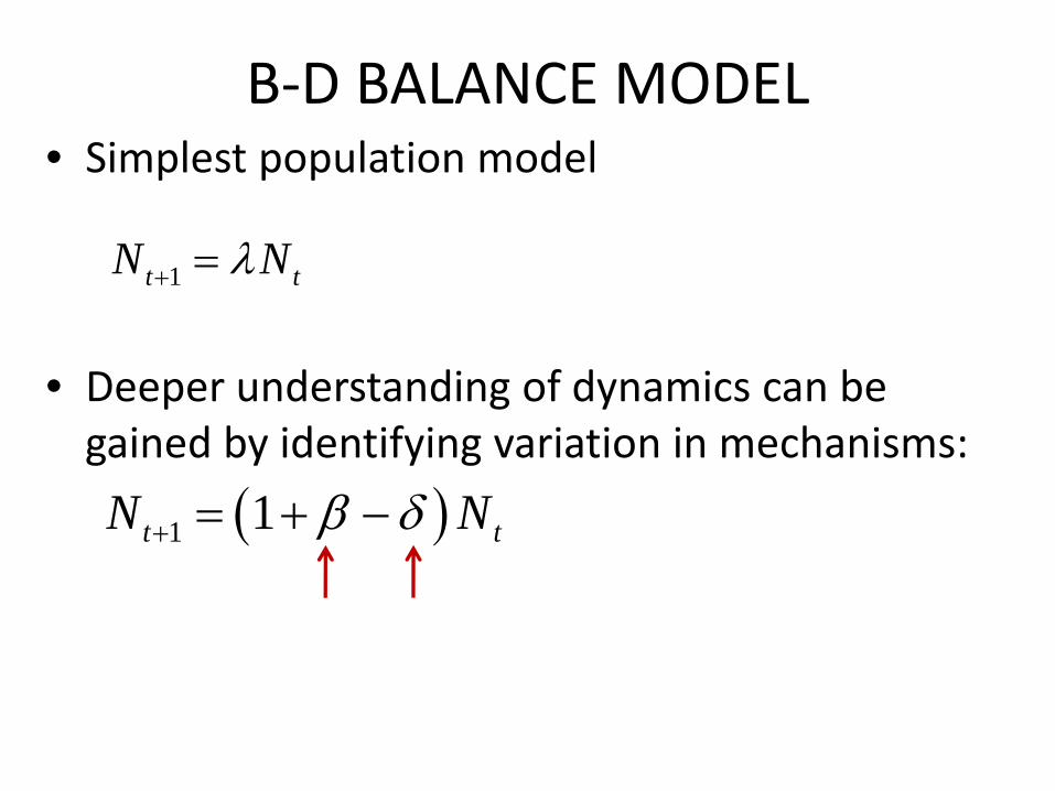
B‐D BALANCE MODEL• Simplest population model

• Deeper understanding of dynamics can be gained by identifying variation in mechanisms: 

( )1 1t tN Nβ δ+ = + −

1t tN Nλ+ =

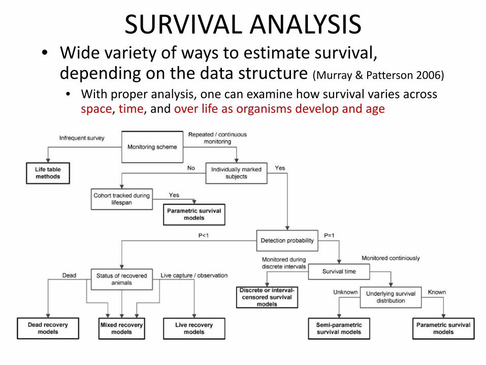
SURVIVAL ANALYSIS• Wide variety of ways to estimate survival, depending on the data structure (Murray & Patterson 2006)

• With proper analysis, one can examine how survival varies across space, time, and over life as organisms develop and age

KNOWN FATE STUDIES

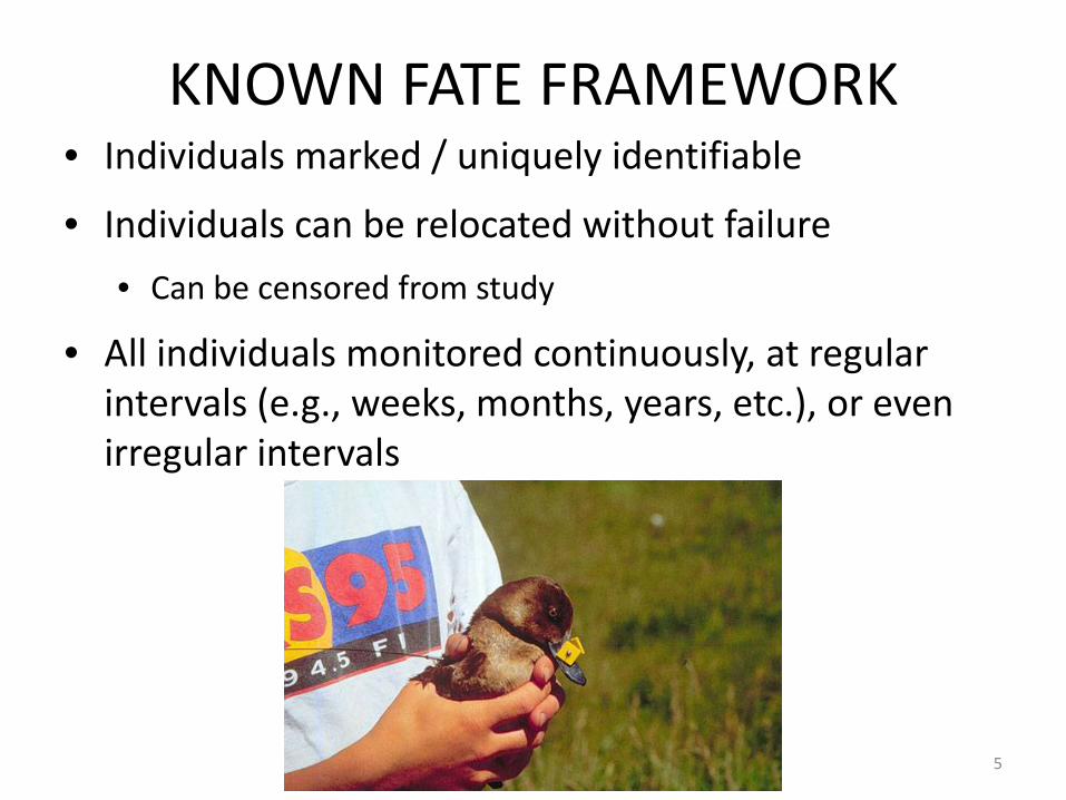
KNOWN FATE FRAMEWORK• Individuals marked / uniquely identifiable

• Individuals can be relocated without failure

• Can be censored from study

• All individuals monitored continuously, at regular intervals (e.g., weeks, months, years, etc.), or even irregular intervals

5

TERMINOLOGY• Known Fate Survival Analysis – if monitoring is continuous, it 

might also be called time to event analysis, failure time analysis

• At risk – number of individuals exposed to detectablemortality in a study (emigration out of study area is grounds for removal from the at‐risk group)

• Right censor – to remove an individual from the at‐risk group for some reason unrelated to mortality (individual remains in at‐risk group until it is censored)

• Staggered Entry — the addition of subjects to the at‐risk group during the course of the study (a.k.a. left truncation)

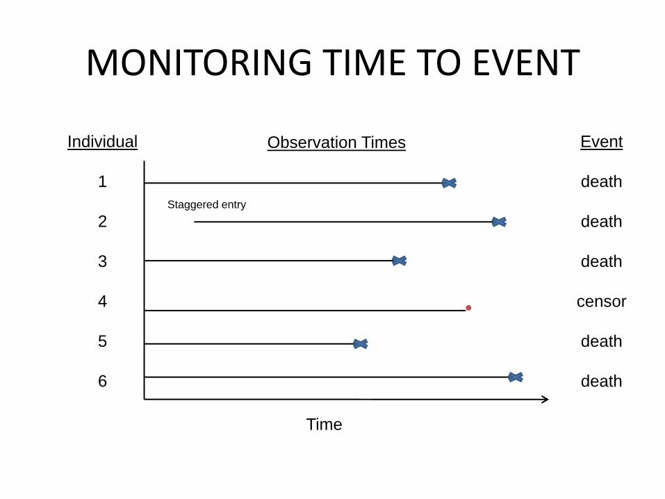
MONITORING TIME TO EVENT

Individual

1

2

3

4

5

6

Time

Observation Times Event

death

death

death

censor

death

death

Staggered entry

FUNCTIONS• Density function f(t) – PDF of failure times or mortality 

times; F(t) is the associated CDF 

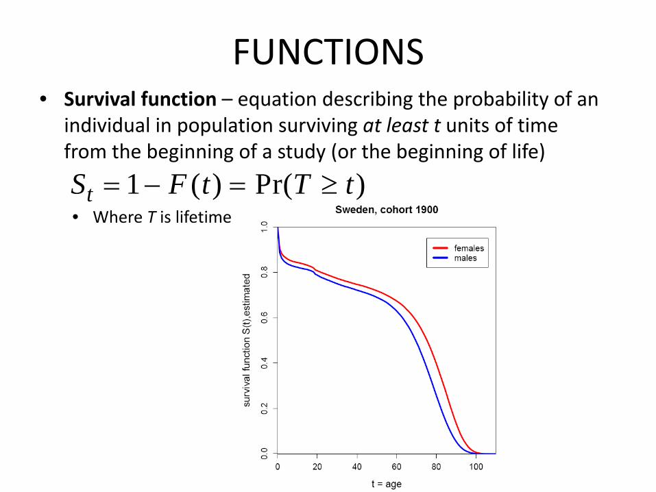
FUNCTIONS• Survival function – equation describing the probability of an 

individual in population surviving at least t units of time from the beginning of a study (or the beginning of life)

• Where T is lifetime

1 ( ) Pr( )tS F t T t= − = ≥

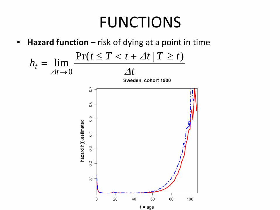
FUNCTIONS• Hazard function – risk of dying at a point in time

0

Pr( | )limtt

t T t t T thtΔ

ΔΔ→

≤ < + ≥=

FUNCTION IDENTITIES

• Cumulative Hazard function – cumulated risk of dying from beginning of life up to a point in time

• Continuous time function

[ ]'

( )

( )

ln

tt

t t

t t

f thS

f t h S

h S

=

=

= −

0

tt xH h dx= ∫

& lntHt t tS e H S−= = −

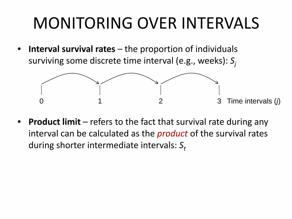
MONITORING OVER INTERVALS• Interval survival rates – the proportion of individuals 

surviving some discrete time interval (e.g., weeks): Sj

• Product limit – refers to the fact that survival rate during any interval can be calculated as the product of the survival rates during shorter intermediate intervals: St

0 1 2 3 Time intervals (j)

WORDS OF CAUTION• In large study areas, mobile individuals may go “missing” then “found” later

• Do not reconstruct unobserved observation times! 

• Censor from data set then re‐enter under staggered entry

• Or if common, use capture‐mark‐recapture analysis

• If individuals are separately monitored at irregular intervals

• Use Nest Survival models to estimate survival (next lecture)

• A special type of known fate analysis

• Commonly needed in large scale studies where logistics are difficult

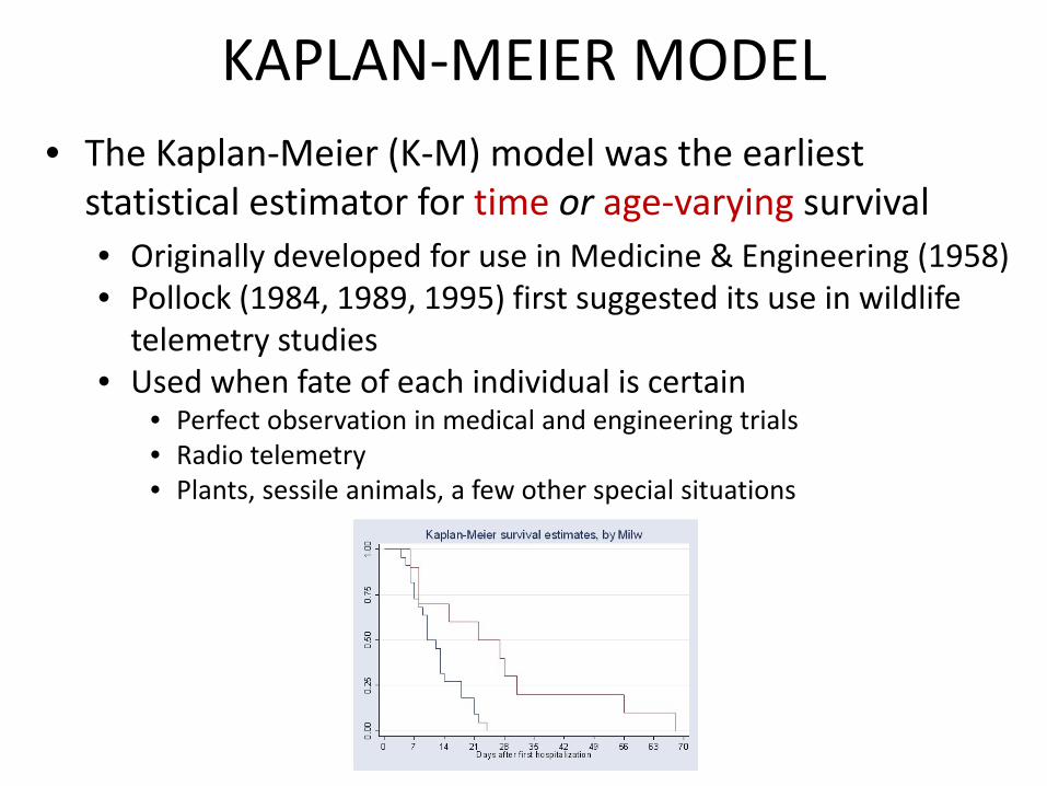
KAPLAN‐MEIER MODEL• The Kaplan‐Meier (K‐M) model was the earliest statistical estimator for time or age‐varying survival• Originally developed for use in Medicine & Engineering (1958)• Pollock (1984, 1989, 1995) first suggested its use in wildlife telemetry studies

• Used when fate of each individual is certain• Perfect observation in medical and engineering trials• Radio telemetry• Plants, sessile animals, a few other special situations

K‐M VARIABLES‐ discrete time points when deaths (failures) occur 

(alternatively use regular sampling periods e.g., weeks, months, etc.)

‐ number of individuals at risk at these time points

‐ number of deaths recorded at these time points

0 1, , , ja a a…

0 1, , , jr r r…

0 1, , , jd d d…

a r d censored added0 7 0 1 0

1 6 0 0 5

2 11 1 0 0

3 10 0 0 6

4 16 1 0 0

5 15 0 0 0

6 15 1 0 0

7 14 0 0 0

8 14 3 0 0

Bobwhite survival in fall 1986 (Pollock 1989)

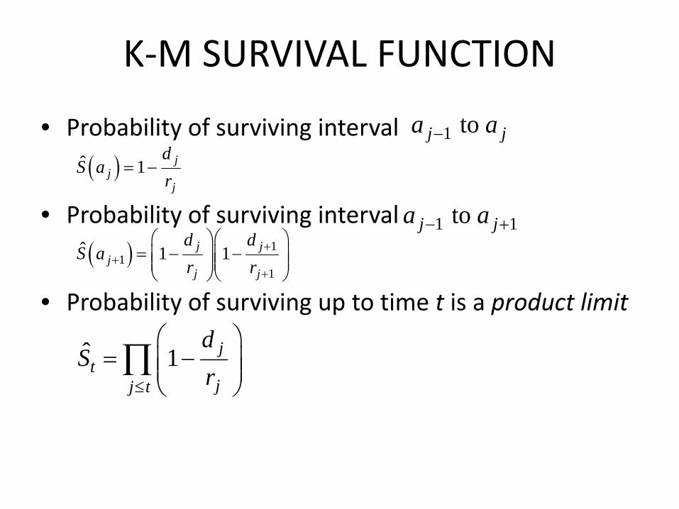
K‐M SURVIVAL FUNCTION

• Probability of surviving interval 

• Probability of surviving interval 

• Probability of surviving up to time t is a product limit

1 to j ja a−

1 1to j ja a− +

( )ˆ 1 jj

j

dS a

r= −

( ) 11

1

ˆ 1 1j jj

j j

d dS a

r r+

++

⎛ ⎞⎛ ⎞= − −⎜ ⎟⎜ ⎟⎜ ⎟⎜ ⎟⎝ ⎠⎝ ⎠

ˆ 1 jt

jj t

dS

r≤

⎛ ⎞= −⎜ ⎟⎜ ⎟

⎝ ⎠∏

K‐M SURVIVALa r d S(j) S(t) censored added0 7 0 1.0000 1.0000 1 0

1 6 0 1.0000 1.0000 0 5

2 11 1 0.9091 0.9091 0 0

3 10 0 1.0000 0.9091 0 6

4 16 1 0.9375 0.8523 0 0

5 15 0 1.0000 0.8523 0 0

6 15 1 0.9333 0.7955 0 0

7 14 0 1.0000 0.7955 0 0

8 14 3 0.7857 0.6250 0 0

Bobwhite survival in fall 1986 (Pollock 1989)

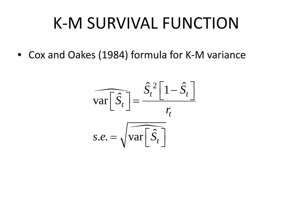
K‐M SURVIVAL FUNCTION

• Cox and Oakes (1984) formula for K‐M variance

2ˆ ˆ1ˆvar

ˆ. . var

t tt

t

t

S SS

r

s e S

⎡ ⎤−⎣ ⎦⎡ ⎤ =⎣ ⎦

⎡ ⎤= ⎣ ⎦

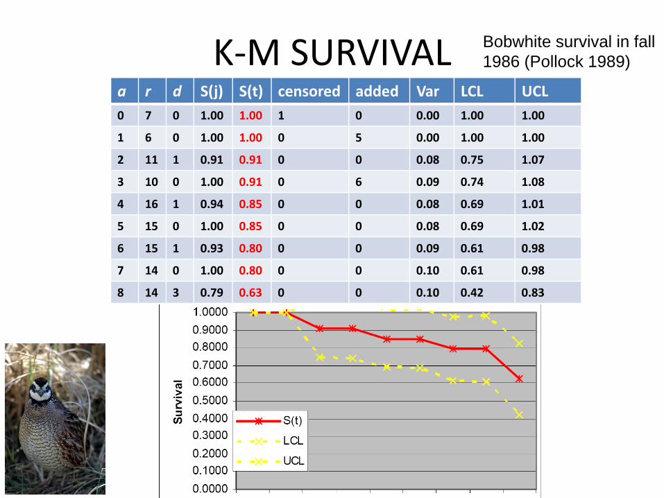
K‐M SURVIVALa r d S(j) S(t) censored added Var LCL UCL0 7 0 1.00 1.00 1 0 0.00 1.00 1.00

1 6 0 1.00 1.00 0 5 0.00 1.00 1.00

2 11 1 0.91 0.91 0 0 0.08 0.75 1.07

3 10 0 1.00 0.91 0 6 0.09 0.74 1.08

4 16 1 0.94 0.85 0 0 0.08 0.69 1.01

5 15 0 1.00 0.85 0 0 0.08 0.69 1.02

6 15 1 0.93 0.80 0 0 0.09 0.61 0.98

7 14 0 1.00 0.80 0 0 0.10 0.61 0.98

8 14 3 0.79 0.63 0 0 0.10 0.42 0.83

Bobwhite survival in fall 1986 (Pollock 1989)

LOG‐RANK TEST• Used to test whether two (or more) survival functions are equal• For two groups, the test is based on the summed (over time) observed minus expected number of deaths for a given group and its variance

• Compute either a Z or χ2 statistic and associated p‐value 

K‐M SURVIVAL ASSUMPTIONS• Individuals randomly sampled within groups (age, sex, location)

• Time or interval of death is known (unless censored)

• Detection probability  = 1

• Individual fates are independent of one another

• Capture/marking does not influence survival

• Censoring is random (independent of fate)

• Staggered entry assumes that newly tagged individuals have the same survival function as previously tagged

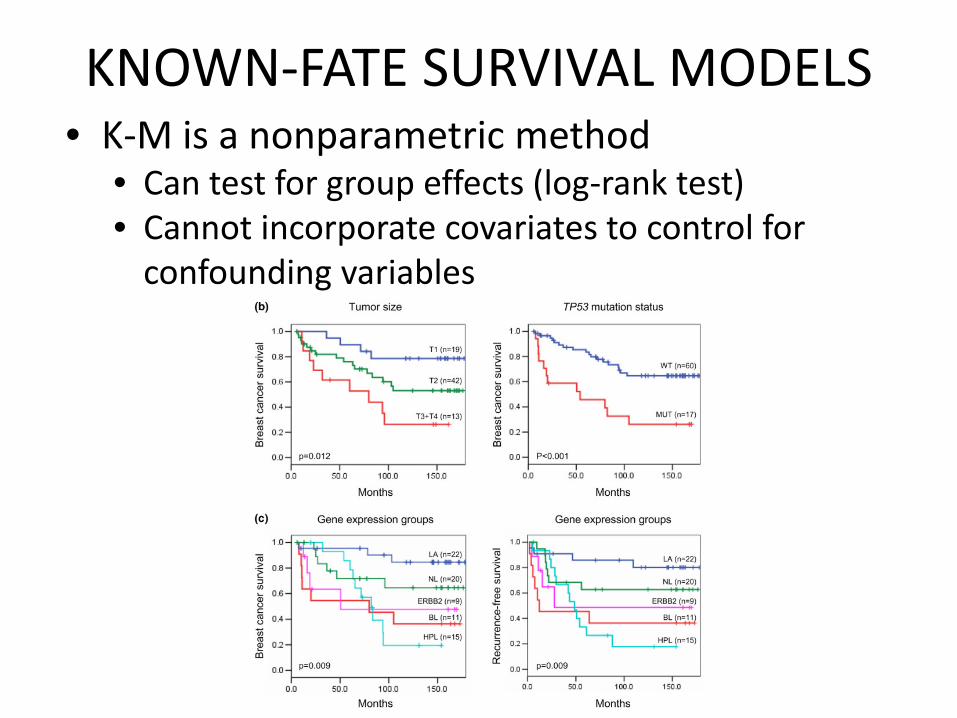
KNOWN‐FATE SURVIVAL MODELS• K‐M is a nonparametric method

• Can test for group effects (log‐rank test)• Cannot incorporate covariates to control for confounding variables

KNOWN‐FATE SURVIVAL MODELS• Semi‐parametric proportional hazard models

• Cox Proportional Hazards

• Useful for analysis of cause‐specific mortality (Heisey and Patterson 2006)

• Useful for examining effects of time‐varying covariates

0

0

( )ln ln ( )

tt

t t

h h t eh h t== +

i βX

βX

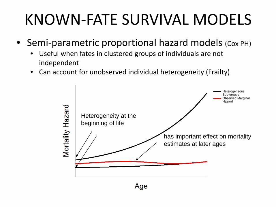
KNOWN‐FATE SURVIVAL MODELS• Semi‐parametric proportional hazard models (Cox PH)

• Useful when fates in clustered groups of individuals are not independent

• Can account for unobserved individual heterogeneity (Frailty)

HeterogeneousSub-groupsObserved Marginal Hazard

Heterogeneity at the beginning of life

has important effect on mortality estimates at later ages

25

Case Study: Black‐Legged Kittiwakes

Lise Aubry

Jean Joachim

•26

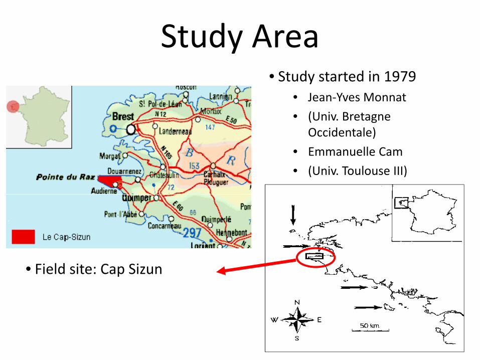
Study Area• Study started in 1979

• Jean‐Yves Monnat 

• (Univ. Bretagne Occidentale)

• Emmanuelle Cam 

• (Univ. Toulouse III)

• Field site: Cap Sizun

27

Follow Up• 5 color bands: 8 possible colors (W, N, B, J, 0, R,V, P)

• 2 are specific to the banding cohort 

• 3 other bands in the other leg

• 1 metal band (Museum of Natural History, Paris)

• After first reproduction, all birds sighted every year until mortality

WOPBV

Lise Aubry

KITTIWAKE SURVIVAL• Cox proportional hazard models

• With time‐varying covariates & Frailty term

1

tHt

tx

t

S eSP

S

−

−

=

=

Aubry et al. submitted

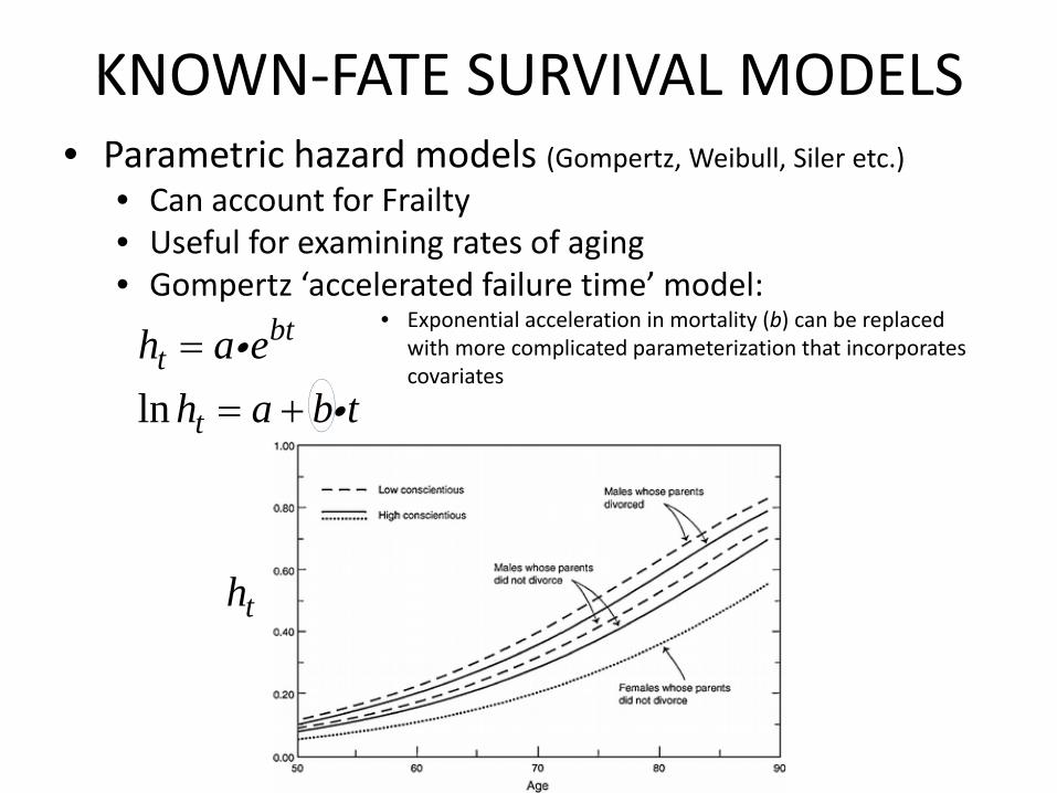
KNOWN‐FATE SURVIVAL MODELS• Parametric hazard models (Gompertz, Weibull, Siler etc.)

• Can account for Frailty• Useful for examining rates of aging• Gompertz ‘accelerated failure time’ model:

• Exponential acceleration in mortality (b) can be replaced with more complicated parameterization that incorporates covariates

ln

btt

t

h a eh a b t== +i

i

th

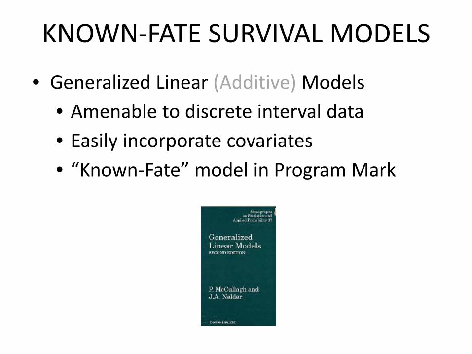
KNOWN‐FATE SURVIVAL MODELS

• Generalized Linear (Additive) Models• Amenable to discrete interval data• Easily incorporate covariates• “Known‐Fate” model in Program Mark

GLM APPROACH

• K‐M model

• Write things in terms of survival (instead of death)

• Where yj is the number surviving interval j and nj is the number at risk during interval j

ˆ jt

jj t

yS

n≤

=∏

ˆ 1 jt

jj t

dS

r≤

⎛ ⎞= −⎜ ⎟⎜ ⎟

⎝ ⎠∏

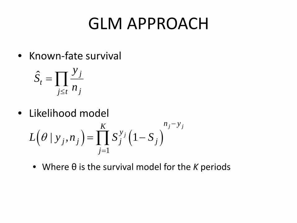
GLM APPROACH

• Known‐fate survival

• Likelihood model

• Where θ is the survival model for the K periods

( ) ( )1

| , 1j j

j

n yKy

j j j jj

L y n S Sθ−

=

= −∏

ˆ jt

jj t

yS

n≤

=∏

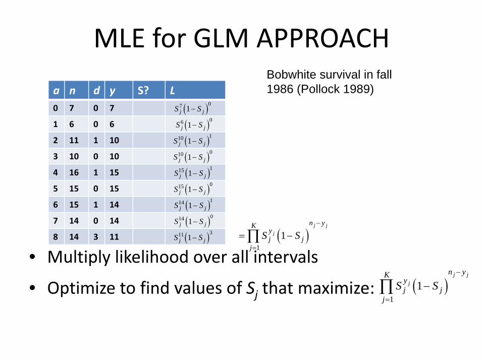
MLE for GLM APPROACH

• Multiply likelihood over all intervals

• Optimize to find values of Sj that maximize:

a n d y S? L0 7 0 7

1 6 0 6

2 11 1 10

3 10 0 10

4 16 1 15

5 15 0 15

6 15 1 14

7 14 0 14

8 14 3 11

Bobwhite survival in fall 1986 (Pollock 1989)

( )07 1j jS S−

( )06 1j jS S−

( )110 1j jS S−

( )010 1j jS S−

( )115 1j jS S−

( )015 1j jS S−

( )114 1j jS S−

( )014 1j jS S−

( )311 1j jS S− ( )1

1j j

j

n yKyj j

jS S

−

=

= −∏

( )1

1j j

j

n yKyj j

jS S

−

=

−∏

MLE for GLM APPROACH

• Multiply likelihood over all intervals

• Optimize to find values of Sj that maximize:

• (Note: Easier to optimize log‐likelihood) 

a n d y S(t) L0 7 0 7 1.00

1 6 0 6 1.00

2 11 1 10 0.91

3 10 0 10 0.91

4 16 1 15 0.85

5 15 0 15 0.85

6 15 1 14 0.80

7 14 0 14 0.80

8 14 3 11 0.63

Bobwhite survival in fall 1986 (Pollock 1989)

( )07 1j jS S−

( )06 1j jS S−

( )110 1j jS S−

( )010 1j jS S−

( )115 1j jS S−

( )015 1j jS S−

( )114 1j jS S−

( )014 1j jS S−

( )311 1j jS S− 121.9 10−= ×

( )1

1j j

j

n yKyj j

jS S

−

=

−∏

MLE for GLM APPROACH

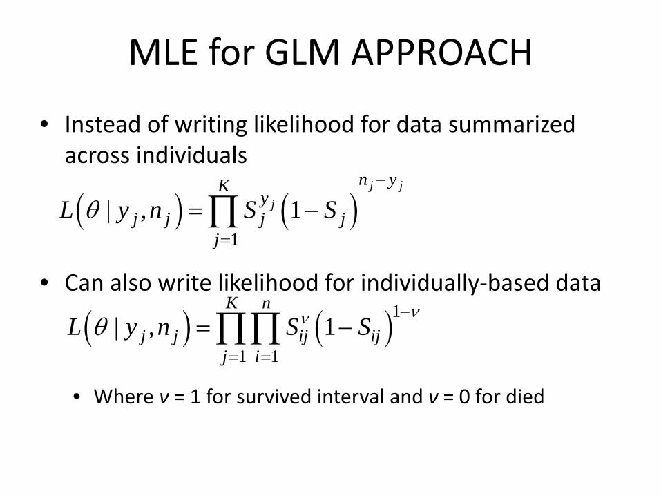
• Instead of writing likelihood for data summarized across individuals

• Can also write likelihood for individually‐based data

• Where ν = 1 for survived interval and ν = 0 for died

( ) ( )1

| , 1j j

j

n yKy

j j j jj

L y n S Sθ−

=

= −∏

( ) ( )11 1

| , 1K n

j j ij ijj i

L y n S Sννθ−

= =

= −∏∏

MLE for GLM APPROACH

• Multiply likelihood over all rows (observations)

• Optimize to find values of Sij that maximize:

• Or sum & optimize log‐likelihood: 

a id f S? L. . . . .

1 1 1

1 2 1

1 3 1

1 4 1

2 1 1

2 2 0

2 3 0

2 4 1

Bobwhite survival in fall 1986 (Pollock 1989)

( )01 1ij ijS S−

( )11 1

1K n

ij ijj i

S Sνν −

= =

= −∏∏

( )11 1

1K n

ij ijj i

S Sνν −

= =

−∏∏

( )01 1ij ijS S−

( )01 1ij ijS S−

( )01 1ij ijS S−

( )01 1ij ijS S−

( )01 1ij ijS S−

( )10 1ij ijS S−

( )10 1ij ijS S−

( ) ( ) ( )1 1

ln | , ln (1 ) 1K n

j j ij ijj i

L y n S Sθ ν ν= =

⎡ ⎤ = + − −⎣ ⎦ ∑∑

MLE for GLM APPROACH• MLE estimation of a GLM for survival over intervals is an extension of the binomial likelihood (day 1 of course)

• MLE of a GLM provides greater flexibility to model variation in survival

• Constant survival S(.)

• K‐M can only model S(t)

• Categorical factors (groups; S(g)) such as sex, habitat, etc.

• Can be implemented as categorical covariates 

• Continuous covariates (body mass, temporal trends, etc.) 

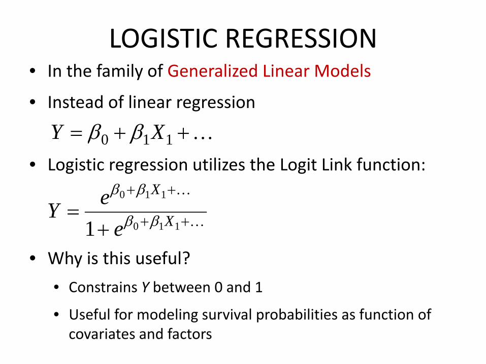
LOGISTIC REGRESSION• In the family of Generalized Linear Models

• Instead of linear regression 

• Logistic regression utilizes the Logit Link function:

• Why is this useful?

• Constrains Y between 0 and 1

• Useful for modeling survival probabilities as function of covariates and factors

0 1 1Y Xβ β= + +…

0 1 1

0 1 11

X

XeY

e

β β

β β

+ +

+ +=+

…

…

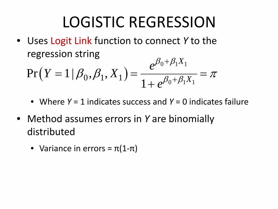
LOGISTIC REGRESSION• Uses Logit Link function to connect Y to the regression string

• Where Y = 1 indicates success and Y = 0 indicates failure

• Method assumes errors in Y are binomially distributed 

• Variance in errors = π(1‐π)

( )0 1 1

0 1 10 1 1Pr 1 | , ,1

X

XeY X

e

β β

β ββ β π+

+= = =+

LOGISTIC REGRESSION• So what’s this Logit Link function all about? 

• The log‐odds of our probability of success is linearly related to the regression string

• This is nice, but it’s for the linearized transformation of the response probability of interest π

0 1 1ln1

Xπ β βπ

⎛ ⎞ = +⎜ ⎟−⎝ ⎠

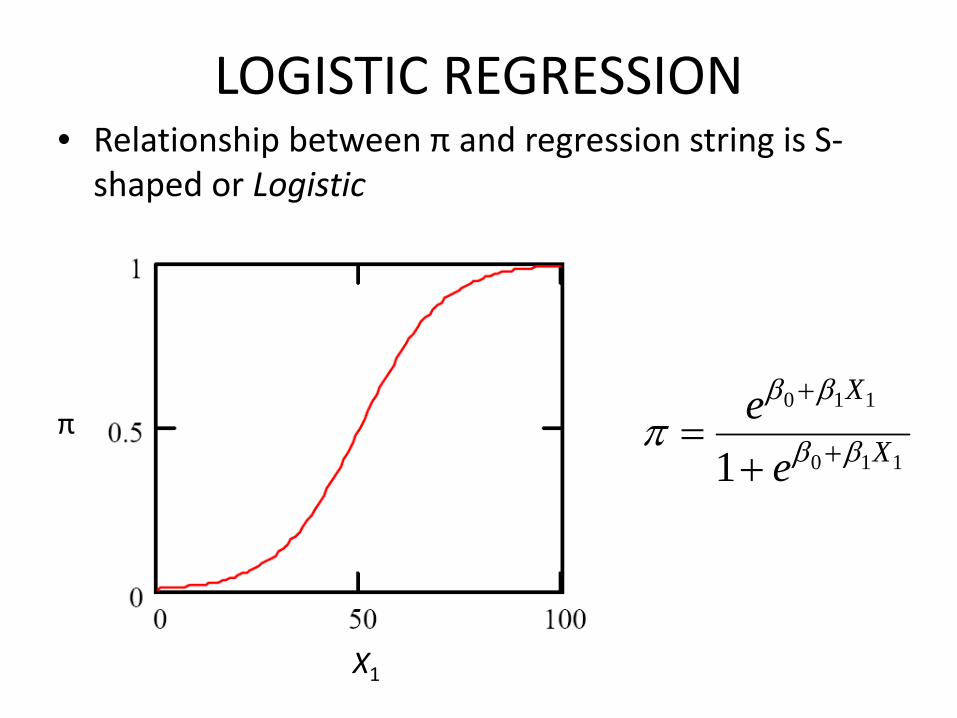
LOGISTIC REGRESSION• Relationship between π and regression string is S‐shaped or Logistic

0 1 1

0 1 11

X

Xe

e

β β

β βπ+

+=+

π

X1

LOGISTIC REGRESSION• Logistic regression fitted to 0‐1 data (failure and success)

π

X1 X2

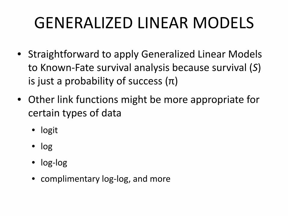
GENERALIZED LINEAR MODELS

• Straightforward to apply Generalized Linear Models to Known‐Fate survival analysis because survival (S) is just a probability of success (π)

• Other link functions might be more appropriate for certain types of data

• logit

• log

• log‐log

• complimentary log‐log, and more

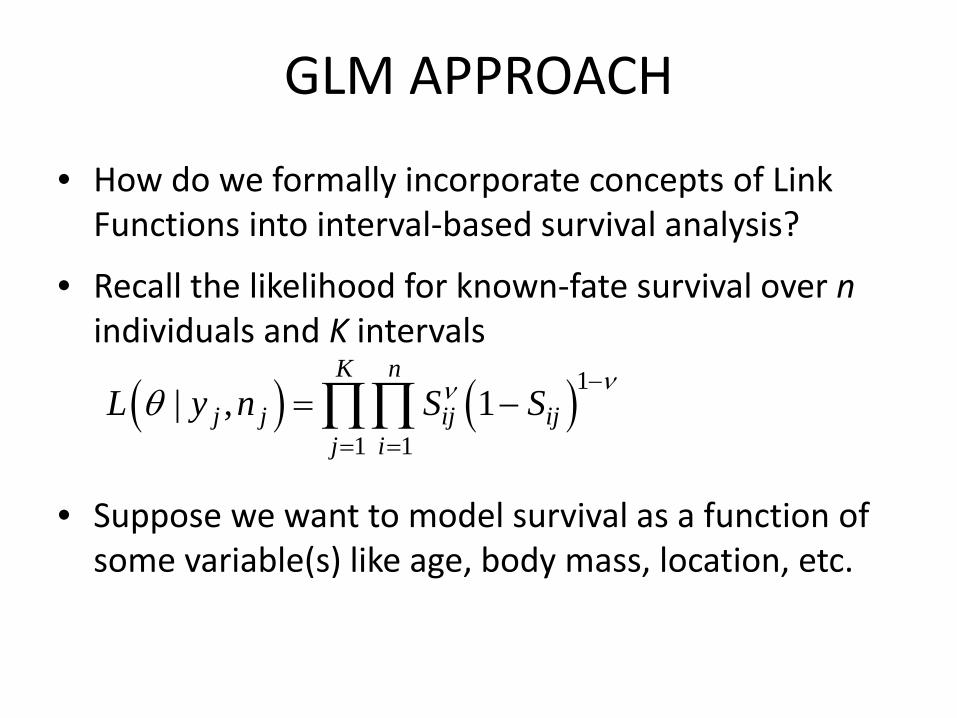
GLM APPROACH

• How do we formally incorporate concepts of Link Functions into interval‐based survival analysis? 

• Recall the likelihood for known‐fate survival over nindividuals and K intervals

• Suppose we want to model survival as a function of some variable(s) like age, body mass, location, etc.

( ) ( )11 1

| , 1K n

j j ij ijj i

L y n S Sννθ−

= =

= −∏∏

GLM APPROACH

• We can do this using the Logit Link, or another link

• This equation can be implemented into the individually‐based survival likelihood

( )0 1 1 0 1 1

0 1 1 0 1 1

1

0 1 ,1 1

, | , 11 1

X XK n

j j X Xj i

e eL y ne e

ν νβ β β β

β β β ββ β−+ +

+ += =

⎛ ⎞ ⎛ ⎞= −⎜ ⎟ ⎜ ⎟

+ +⎝ ⎠ ⎝ ⎠∏∏

0 1 1

0 1 11

X

ij XeS

e

β β

β β

+

+=+

MLE for GLM APPROACH

• Estimates of regression intercepts and slopes (Betas: β) can be estimated with MLE

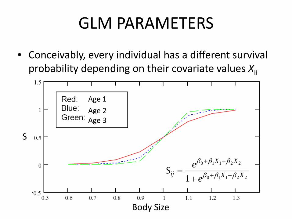
GLM PARAMETERS

• Conceivably, every individual has a different survival probability depending on their covariate values Xij

S

Body Size

Age 1Age 2Age 3

0 1 1 2 2

0 1 1 2 21

X X

ij X XeS

e

β β β

β β β

+ +

+ +=+

GLM PARAMETERS

• Note on interpretation of Betas:

• The parameter β0 determines the baseline intercept

• The parameter βx (x = 1,2, ….j) determines the rate of increase or decrease of the S‐shaped curve for covariate xrelative to β0

• The sign (±) of βx indicates whether the curve ascends or descends

GLM MODELING• Note:

• More than 1 covariate can be examined…structure of regression string in the logit link depends on your hypotheses; for example, does survival depend on:

• Age

• Sex

• Body mass

• Age, body mass, and sex

• Is it constant across time and individuals

• Advanced approaches allow one to control for fate‐dependence within clusters (pairs or families), unobserved individual heterogeneity with random effects

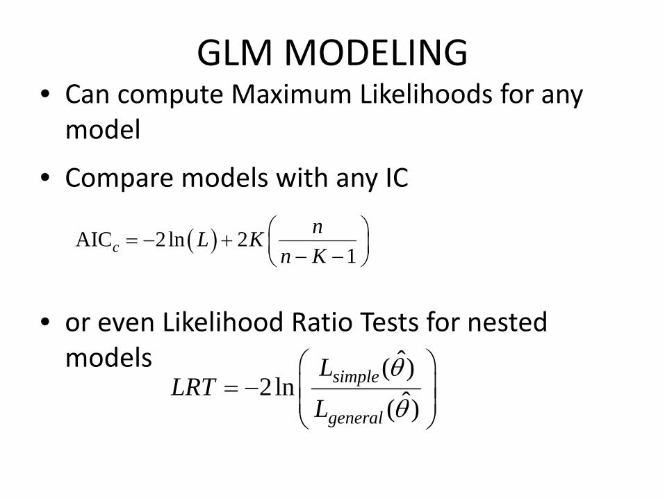
GLM MODELING• Can compute Maximum Likelihoods for any model

• Compare models with any IC     

• or even Likelihood Ratio Tests for nested models

( )AIC 2ln 21

⎛ ⎞= − + ⎜ ⎟− −⎝ ⎠c

nL Kn K

ˆ( )2 ln ˆ( )

simple

general

LLRT

Lθθ

⎛ ⎞= − ⎜ ⎟⎜ ⎟

⎝ ⎠

KNOWN‐FATE IN MARK

• In program MARK, the individual fates should be read in as a Live‐Dead (LD) encounter history

• As a row

• LDLDLDLD

• 10101011

Individual made it to 4th interval and died during 4th interval

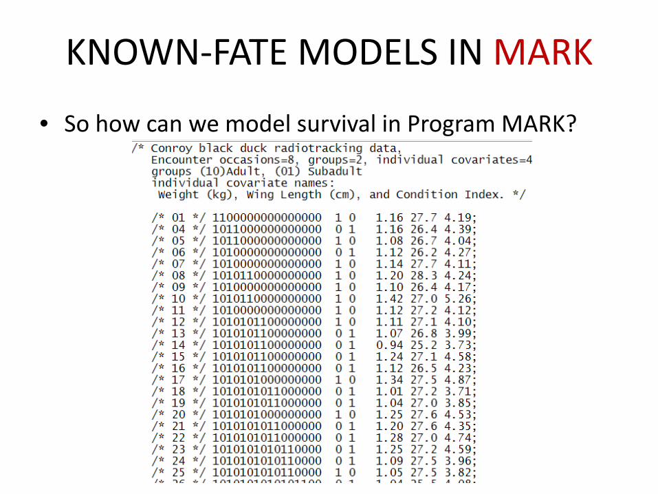
KNOWN‐FATE MODELS IN MARK

• So how can we model survival in Program MARK?

KNOWN‐FATE MODELS IN MARK

KNOWN‐FATE MODELS IN MARK• A variety of pre‐defined models can be examined

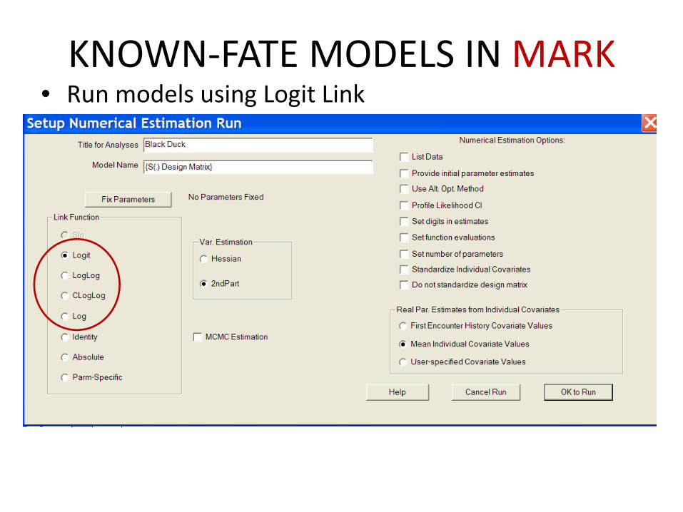
KNOWN‐FATE MODELS IN MARK• Run models using Logit Link

KNOWN‐FATE MODELS IN MARK• Individual covariates in Design Matrix