
CIFE - Stanford Universityzm949qj2893/WP130... · 2016-06-19 · CIFE CENTER FOR INTEGRATED...
74
CIFECENTER FOR INTEGRATED FACILITY ENGINEERING A Method to Analyze Large Data Sets of Residential Electricity Consumption to Inform Data-Driven Energy Efficiency By Amir Kavousian, Ram Rajagopal & Martin Fischer CIFE Working Paper #WP130 June 2012 STANFORD UNIVERSITY
Transcript of CIFE - Stanford Universityzm949qj2893/WP130... · 2016-06-19 · CIFE CENTER FOR INTEGRATED...

CIFECENTER FOR INTEGRATED FACILITY ENGINEERING
A Method to Analyze Large Data Sets of Residential Electricity
Consumption to Inform Data-Driven Energy Efficiency
By
Amir Kavousian, Ram Rajagopal & Martin Fischer
CIFE Working Paper #WP130 June 2012
STANFORD UNIVERSITY

COPYRIGHT © 2012 BY Center for Integrated Facility Engineering
If you would like to contact the authors, please write to:
c/o CIFE, Civil and Environmental Engineering Dept., Stanford University
The Jerry Yang & Akiko Yamazaki Environment & Energy Building 473 Via Ortega, Room 292, Mail Code: 4020
Stanford, CA 94305-4020

A METHOD TO ANALYZE LARGE DATA SETS OF RESIDENTIALELECTRICITY CONSUMPTION TO INFORM DATA-DRIVEN ENERGY
EFFICIENCY
Amir Kavousian1,∗ Ram Rajagopal1,2 Martin Fischer1
Abstract. Effective demand-side energy efficiency policies are needed to reduce residential
electricity consumption and its harmful effects on the environment. The first step to devise
such polices is to quantify the potential for energy efficiency by analyzing the factors that
impact consumption. This paper proposes a novel approach to analyze large data sets of
residential electricity consumption to derive insights for policy making and energy efficiency
programming. In this method, underlying behavioral determinants that impact residential
electricity consumption are identified using Factor Analysis. A distinction is made between
long-term and short-term determinants of consumption by developing separate models for
daily maximum and daily minimum consumption and analyzing their differences. Finally,
the set of determinants are ranked by their impact on electricity consumption, using a
stepwise regression model. This approach is then applied on a large data set of smart
meter data and household information as a case example. The results of the models show
that weather, location, floor area, and number of refrigerators are the most significant
determinants of daily minimum (or idle) electricity consumption in residential buildings,
while location, floor area, number of occupants, occupancy rate, and use of electric water
heater are the most significant factors in explaining daily maximum (peak) consumption.
The results of the models are compared with those of previous studies, and the policy
implications of the results are discussed.
1Center for Integrated Facility Engineering, Civil and Environmental Engineering Department, Stanford,CA, 943052Stanford Sustainable Systems Lab, Civil and Environmental Engineering Department, Stanford, CA, 94305∗Corresponding author. Tel.: 1 650 723-4945 ; Fax: 1 650 723-4806; 473 Via Ortega, Room 291, Stanford,CA 94305Email: [email protected]
1
DATA-DRIVEN ENERGY EFFICIENCY 2
1. Introduction
Residential buildings consume 39% of the total electricity in the US, more than any other
sector or building type [65]. Their electricity consumption has increased by 27% from 1990
to 2008 and—provided the expected efficiency gains are realized—is projected to increase by
18% from 2009 to 2035. To meet this demand, 223 Giggawatts of new generating capacity
will be needed between 2010 and 2035, 75% of which is projected to be provided by fossil
fuels [68]. Detailed planning and execution of demand-side energy efficiency programs is
needed to reduce or stabilize residential electricity consumption, and to prevent its harmful
impact on the environment and on energy security [9].
To plan and execute consumption reduction policies and programs effectively, a sound un-
derstanding of the determinants that drive household electricity consumption (such as floor
area, average outside temperature, and number of occupants) is needed [26]. However, be-
cause of lack of easily-accessible, high-resolution consumption data, underlying determinants
of energy use and energy-related behaviors have hardly been examined before [1].
With growing deployment of smart meters and real-time home energy-monitoring services,
data that allow studying such underlying determinants are becoming available (for examples
of studies using high-resolution consumption data, see [8, 64, 47]). However, the methodolo-
gies to analyze the data and infer the results that can be used to support decision making
at the household level have not yet been formalized [1].
To address that gap, this paper proposes a methodology to analyze large data sets of res-
idential electricity consumption to derive insights for policy making and energy efficiency
programming. In particular, it offers a method to disaggregate the impact of structural
determinants (e.g., insulation level of the residence) from behavioral determinants (e.g., oc-
cupant habits). As a case study, we use a large data set of ten-minute interval smart meter
data for 1628 households in the U.S.. The data set is collected over 238 days in 2010, and
DATA-DRIVEN ENERGY EFFICIENCY 3
is supported by an extensive 114-question survey of household data. The household survey
covers information about the climate, location, dwelling, appliances, and occupants.
Using this methodology and the data, this paper develops a model to estimate the impact
of each of the following interventions on residential electricity consumption: (a) behavioral
modifications; (b) improving the efficiency of appliances and electronics; and, (c) improving
the physical characteristics of dwellings. By estimating the amount of reduction achievable
through each of these interventions, one can also infer what portion of residential electricity
consumption is outside the scope of the influence of current methods and programs.
In the following sections, we start with a review of existing models for residential electricity
consumption, followed by our methodology and corresponding model. We then describe the
data and preprocessing methods normally needed to prepare the data for modeling. Next, we
present the results of our model applied to the data set introduced above, while comparing
them with the results of previous studies and commenting on potential causes for discrepancy
among the results. Finally, we suggest the policy implications of the results.
2. Review of Residential Electricity Consumption Modeling
Several studies in the past have proposed models to explain determinants of residential
electricity consumption. One of the first groups of studies in this regard were economics-
oriented studies that were published in the aftermath of the 1970’s energy crisis. These
studies primarily focused on informing high-level energy conservation policies such as en-
ergy pricing mechanisms and taxation to manage electricity demand, hence reducing the oil
consumption and the rate of resource depletion [1, 40]. Therefore, they focused primarily
on explaining the decision making process of the households, and in particular explaining
how the consumers respond to changes in price given their income levels; i.e., whether the
decision to reduce electricity consumption is price-elastic, income-elastic, or neither [12, 60].
The explanatory variables used in these models were primarily socioeconomic factors of the
household, or the ownership of certain high-consumption appliances such as refrigerators or
DATA-DRIVEN ENERGY EFFICIENCY 4
electric water heaters, while the specific contribution of many end uses or physical charac-
teristics of the dwelling were not included in the models. In other words, these models were
mostly top-down models, providing insights into high-level policy design [62]. For examples
of economics-oriented papers see [6, 27, 28, 31, 34, 38, 16, 56].
However, the purpose of our study is to use a large set of explanatory variables to inform
energy efficiency programs that attempt to reduce consumption by addressing the drivers
of consumption and to understand the interaction of these factors [13]. In other words, our
goal is to create a bottom-up model for electricity consumption, which is different from the
goal of the economics-oriented models.
Another group of studies have attempted to create bottom-up models for electricity con-
sumption by disaggregating the total electricity consumption into its constituent parts in a
process called Conditional Demand Analysis (CDA) [2, 5, 11, 36, 24, 41, 46, 50, 62]. These
studies adopt an econometrics perspective, attempting to explain aggregate consumption
data based on a selected stock of appliances. Therefore, the effect of behavior and other
variables such as climate are merged with the effect of appliances, mainly because one goal
of these studies is to minimize the amount of data requirements for end use consumption es-
timation. However, since the effect of occupant behavior is explained in the context of using
a few major appliances, it is not feasible to disaggregate the effect of structural determinants
(e.g., insulation of the house, efficiency of the appliances) from the behavioral aspects (e.g.,
usage levels, conservation efforts of the occupants) using these models.
A third group of studies have analyzed the role of occupants in residential electricity con-
sumption, sometimes with contrasting results: while some studies have estimated that oc-
cupancy and occupant behavior can impact residential energy consumption by a scale of
two (e.g., see [57]), others have observed no significant correlation between occupant behav-
ior and electricity use (e.g., see [15]). Most behavioral analysis studies have only analyzed
the behavioral determinants1 of electricity consumption [60]; the few studies that have also
1also called “internal” factors in behavioral studies literature
DATA-DRIVEN ENERGY EFFICIENCY 5
included structural determinants2 use aggregate consumption data or a limited number of
explanatory variables. These studies normally adopt a behavioral sciences or behavioral
economics point of view. For examples of these studies see [3, 35, 55].
3. Summary of Limitations of Existing Models
For our purposes, we need a bottom-up model that can make use of high-resolution electricity
consumption data and a large set of information about the households. Existing models
cannot support the use of high-resolution data due to:
(a) Use of aggregate (low-resolution) consumption data: Most studies in the past
have used monthly billing data, mainly because the advanced metering technologies of today
were not easily accessible [2, 5, 11, 36, 24, 41, 46, 50, 62]. However, Masiello and Parker
[47] show that residential electricity consumption has strong temporal variation, which is
not captured with low-resolution consumption data such as monthly bills.
(b) Partial set of explanatory variables: A large number of previous studies have
analyzed only a partial set of residential electricity consumption determinants; e.g., only
appliance stock, weather conditions, or behavioral factors [12, 60]. However, the interaction
between different factors (e.g., the relationship between weather, appliance load, lighting
load, and heating load) offer considerable potential for improving energy efficiency [1]. An-
other limitation of some of the previous studies is the use of “bundle” variables (such as zip
code) that combine (hence obscure) the effect of several underlying determinants.
(c) No distinction between “idle” consumption of the house and peak consump-
tion: Most studies in the past have either looked at peak consumption (mostly at the utility
level) or the total electricity load. However, understanding the lower limit of electricity con-
sumption (i.e., the part of consumption that is almost constant, regardless of active end uses)
2also called “external” or ”contextual” factors in behavioral studies literature

DATA-DRIVEN ENERGY EFFICIENCY 6
enables policy makers and planners to quantify the potential for energy efficiency. In this pa-
per we also show that the distinction between idle and maximum consumption distinguishes
the ways in which different factors impact electricity consumption.
(d) Using energy intensity as the only indicator for analyzing electricity con-
sumption: Most studies have used energy intensity (kWh per square foot) as the metric
to measure residential electricity consumption [6, 27, 28, 31, 34, 38, 16]. This designation
implies that, for example, a refrigerator in a 2000 sq.ft house will consume twice as much as
the same refrigerator in a 1000 sq.ft house, even when all other factors are held constant. In-
stead, we scale only those factors whose consumption is dependent on floor area by the area
of the house (e.g., lighting and heating loads), and use the actual kWh value for other factors.
The following section describes our proposed solution to address these shortcomings.
4. Model Setup
Our proposed model addresses the limitations of existing models by: (a) classifying ex-
planatory variables based on their physical properties, and their interaction with each other
and with electricity consumption; (b) selecting the most significant variables; (c) identify-
ing different features of high-resolution smart meter data that offer a better understanding
of residential electricity consumption; and (d) fitting the model via a stepwise method to
identify the ranks of most important variables.
4.1. Explanatory Variables. Through a review of the residential electricity consumption
models and building sciences literature [26], we identified four major categories of residential
electricity consumption determinants (Table 2):
(1) Weather and location. Examples: daily outdoor temperature and climate zone;
these determinants are normally outside the scope of influence of the household.
DATA-DRIVEN ENERGY EFFICIENCY 7
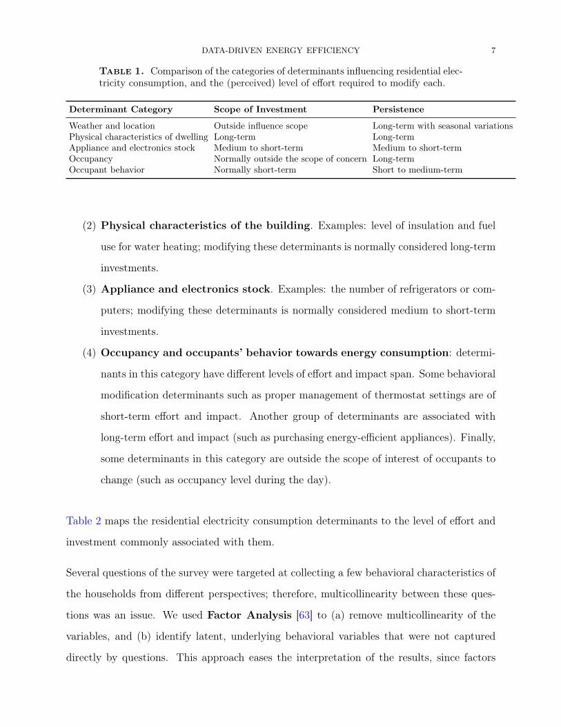
Table 1. Comparison of the categories of determinants influencing residential elec-tricity consumption, and the (perceived) level of effort required to modify each.
Determinant Category Scope of Investment Persistence
Weather and location Outside influence scope Long-term with seasonal variationsPhysical characteristics of dwelling Long-term Long-termAppliance and electronics stock Medium to short-term Medium to short-termOccupancy Normally outside the scope of concern Long-termOccupant behavior Normally short-term Short to medium-term
(2) Physical characteristics of the building. Examples: level of insulation and fuel
use for water heating; modifying these determinants is normally considered long-term
investments.
(3) Appliance and electronics stock. Examples: the number of refrigerators or com-
puters; modifying these determinants is normally considered medium to short-term
investments.
(4) Occupancy and occupants’ behavior towards energy consumption: determi-
nants in this category have different levels of effort and impact span. Some behavioral
modification determinants such as proper management of thermostat settings are of
short-term effort and impact. Another group of determinants are associated with
long-term effort and impact (such as purchasing energy-efficient appliances). Finally,
some determinants in this category are outside the scope of interest of occupants to
change (such as occupancy level during the day).
Table 2 maps the residential electricity consumption determinants to the level of effort and
investment commonly associated with them.
Several questions of the survey were targeted at collecting a few behavioral characteristics of
the households from different perspectives; therefore, multicollinearity between these ques-
tions was an issue. We used Factor Analysis [63] to (a) remove multicollinearity of the
variables, and (b) identify latent, underlying behavioral variables that were not captured
directly by questions. This approach eases the interpretation of the results, since factors
DATA-DRIVEN ENERGY EFFICIENCY 8
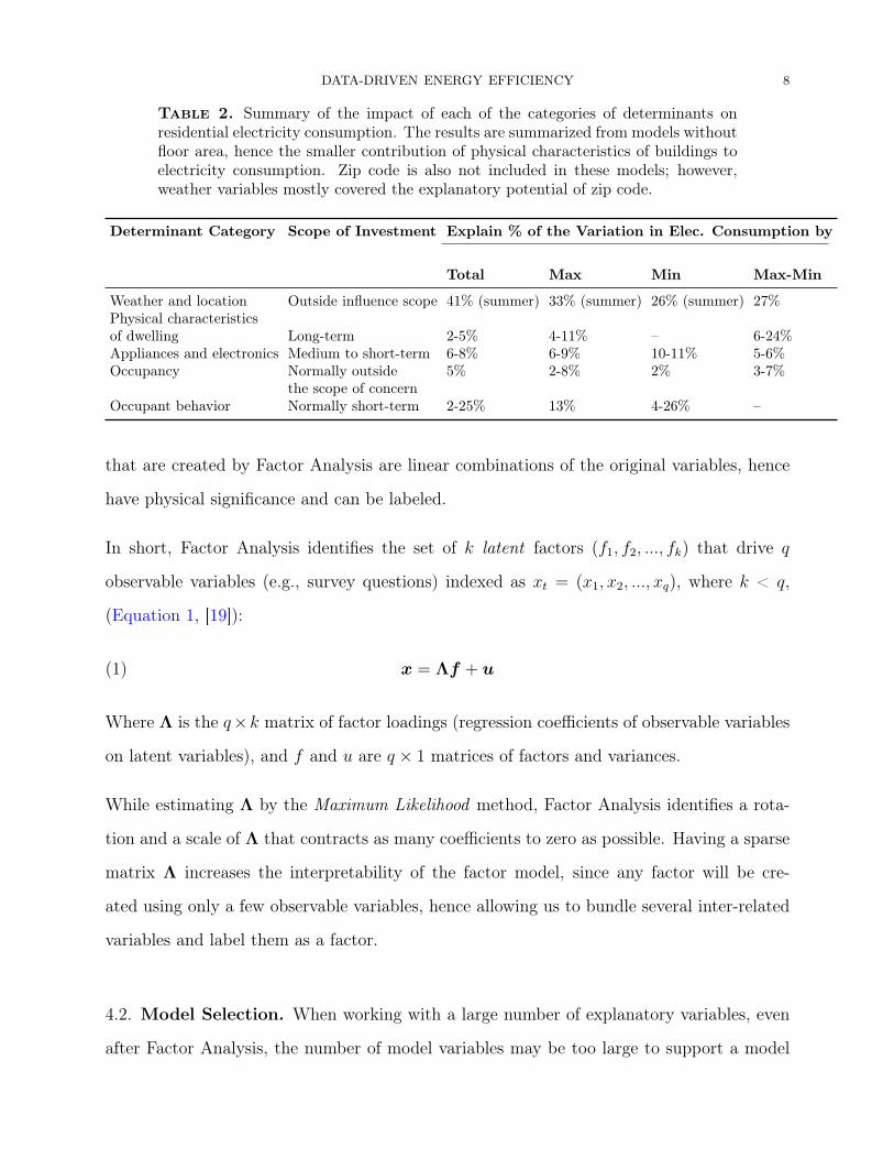
Table 2. Summary of the impact of each of the categories of determinants onresidential electricity consumption. The results are summarized from models withoutfloor area, hence the smaller contribution of physical characteristics of buildings toelectricity consumption. Zip code is also not included in these models; however,weather variables mostly covered the explanatory potential of zip code.
Determinant Category Scope of Investment Explain % of the Variation in Elec. Consumption by
Total Max Min Max-Min
Weather and location Outside influence scope 41% (summer) 33% (summer) 26% (summer) 27%Physical characteristicsof dwelling Long-term 2-5% 4-11% – 6-24%Appliances and electronics Medium to short-term 6-8% 6-9% 10-11% 5-6%Occupancy Normally outside 5% 2-8% 2% 3-7%
the scope of concernOccupant behavior Normally short-term 2-25% 13% 4-26% –
that are created by Factor Analysis are linear combinations of the original variables, hence
have physical significance and can be labeled.
In short, Factor Analysis identifies the set of k latent factors (f1, f2, ..., fk) that drive q
observable variables (e.g., survey questions) indexed as xt = (x1, x2, ..., xq), where k < q,
(Equation 1, [19]):
(1) x = Λf + u
Where Λ is the q×k matrix of factor loadings (regression coefficients of observable variables
on latent variables), and f and u are q × 1 matrices of factors and variances.
While estimating Λ by the Maximum Likelihood method, Factor Analysis identifies a rota-
tion and a scale of Λ that contracts as many coefficients to zero as possible. Having a sparse
matrix Λ increases the interpretability of the factor model, since any factor will be cre-
ated using only a few observable variables, hence allowing us to bundle several inter-related
variables and label them as a factor.
4.2. Model Selection. When working with a large number of explanatory variables, even
after Factor Analysis, the number of model variables may be too large to support a model

DATA-DRIVEN ENERGY EFFICIENCY 9
that is easy to interpret and statistically stable. Furthermore, it is important to identify
the most important variables (those variables that contribute the most to the variation in
consumption) to inform future data collection efforts and avoid collecting data that will
not significantly contribute to the accuracy of the model. Our preferred method for model
selection is forward stepwise selection [29] because (a) it ranks the variables based on their
importance; and (b) in sequentially adding variables to the model, it ensures multicollinearity
does not negatively affect the performance of the model.
The forward stepwise algorithm starts with the mean value of the consumption (i.e., the
intercept) and then sequentially adds to the model the determinant that best improves the
fit, as measured by the Akaike Information Criteria (AIC, [52]), given by Equation 2:
(2) AIC = −2. logL+ 2edf
where L is the likelihood and edf the equivalent degrees of freedom (i.e., the number of free
parameters for usual parametric models) of fit. The use of AIC to evaluate the fit at every
step of adding a new variable to the mix prevents over-fitting the model.
4.3. Response Variables. We considered four different features of the hourly electricity
consumption data: daily average, minimum, maximum, and maximum-minus-minimum (also
called “range”). For example, daily minimum and daily maximum consumption refer to the
lowest and highest values of the hourly consumption data as recorded by the meter (2
extreme values from 24 daily values). Each feature was then used as the response variable
in a separate regression model. Such approach enables disaggregating the role of structural
versus behavioral determinants of consumption.
4.4. Regression Model. We developed a weighted regression model to explain the variation
in household electricity consumption. Those determinants whose contribution to electricity
consumption has a linear relationship with floor area are multiplied by the floor area of

DATA-DRIVEN ENERGY EFFICIENCY 10
the residence. For example, poor insulation will cause larger houses to waste more energy
(through increased envelope surface) compared to smaller houses. On the other hand, a
refrigerator has the same consumption level regardless of the size of the house. The majority
of previous papers that we reviewed regress energy intensity (kWh/sq.ft) on all end uses.
The regression equation of our model is given by:
(3) yj = β0j +M∑i=1
βijXij + Aj.
K∑i=M+1
βijXij + εj,
where yj is the electricity consumption (kWh) of household j, Xij is the value of the deter-
minant number i for household j, and βij is the regression coefficient for that determinant.
M is the number of variables (household features) that do not depend on floor area, while
K is the total number of variables, and ε is the error term.
After selecting the p variables that contribute the most to the model fit using forward stepwise
model selection (explained above), and multiplying the floor-area-dependent variables by the
square foot value of the dwelling, we formed a single matrixX and formed the final regression
model as:
(4) y = Xβ + ε,
where y is the n× 1 vector of household consumption values (in kWh), X is a n× (p + 1)
matrix where p is the number of selected variables, ε is a n× 1 vector of residuals, and β is
the (p+ 1)× 1 vector of regression coefficients.
To summarize, our model enables working with large data sets of electricity consumption
data and large household surveys, by (a) using several indicators (electricity consumption
features or load characteristics) in addition to the aggregate load that help understand
different aspects of consumption (e.g., long-term steady idle load versus short-term volatile
peak load); and, (b) choosing variables that contribute the most to those load characteristics.

DATA-DRIVEN ENERGY EFFICIENCY 11
Our model also introduces a novel approach to understanding the effect of appliances more
accurately by (c) properly considering the effect of floor area.
5. Data Summary and Preprocessing
We applied our model to a data set of ten-minute interval smart meter data for 1628 house-
holds, collected over 238 days starting from February 28, 2010 through October 23, 2010.
Detailed data about household characteristics were available via a 114-questions online sur-
vey. The survey questions covered a wide range of characteristics including climate and
location, building characteristics, appliances and electronics stock, demographics, and be-
havioral characteristics of occupants. The following sections explain the data in more detail.
5.1. Consumption Data. Participant households were selected through a voluntary en-
rollment in the program, and were provided with a device that recorded the electricity
consumption of the household every ten minutes and sent the data to a central server to be
stored. The device installation and server costs were covered by the experiment adminis-
trators, and participants volunteered to participate merely based on their interest (for more
details of the experiment, refer to [33]).
The consumption data were converted to hourly data (a) to ensure that the fluctuations
in electricity consumption are considered, but not obscured by sudden spikes in the con-
sumption; and (b) to compare the results of our models with those of previous studies on
smart meter data and electricity market analysis [44]. Furthermore, we chose not to remove
extreme-consumption households from the sample to ensure that the model captures deter-
minants that are associated with a wide range of consumption volumes. Such a model would
enable the prediction of likely extreme users in other household samples.
5.2. Household Data. The smart meter data were supported with a detailed survey of
geographical and physical characteristics of dwellings as well as appliance stock, occupant

DATA-DRIVEN ENERGY EFFICIENCY 12
Table 3. Summary statistics of the daily maximum, minimum, and average hourlyconsumption, averaged over all users in the case study. The variability in dailyminimum hourly consumption is the lowest, and that of the daily maximum is thelargest.
Variable no. of days Min x̃ x̄ Max sDaily maximum kWh∗ 238 1.7 2.5 2.5 3.5 0.256Daily minimum kWh∗ 238 0.2 0.4 0.4 0.5 0.039Daily average kWh∗ 238 0.5 0.8 0.9 1.2 0.1
*Averaged over all households.
01
23
4
kWh
03/0
1/10
04/0
1/10
05/0
1/10
06/0
1/10
07/0
1/10
08/0
1/10
09/0
1/10
10/0
1/10
11/0
1/10
Daily MaximumDaily AverageDaily Minimum
Figure 1. Comparison of daily average, maximum, and minimum consumption,averaged over all users for each day of the experiment.
profiles, and attitude of occupants towards electricity usage, for a total of 114 questions.
The survey was administered online.

DATA-DRIVEN ENERGY EFFICIENCY 13
Table 4. Distribution of survey questions covering four major categories of house-hold characteristics.
Question Categories No. of Survey QuestionsExternal determinantsClimate and Geography 6
Building Design and ConstructionBuildings 5Home Improvements 12
Building Systems and AppliancesFuel Use 6Appliances 14
OccupantsOccupants age and employment profile 12Energy efficiency habits 14Payment items, method, estimate, feedback 6How informed about appliances’ use 5Motivation level 17Effort to learn energy efficiency actions 7Thermostat setpoint 6Income, age, race, and other personal information 4
Total 114
After collecting the data, 952 households for which reliable smart meter and survey data were
available were selected for the analysis. Less than 3% of survey responses were inconsistent
or missing, for which we imputed data using iterative model-based imputation techniques
([14, 23]). The selected households are located in 419 different zip codes, 140 different
counties, 26 different states, and are spread across all six climate zones defined by the
Department of Energy [65]. California has the largest representation (53% of households)
of all states in the data set. During the data collection process, the weather conditions in
most areas where participant households resided were similar to the 30-year average climatic
conditions; however, some areas, especially in the north east of the U.S., experienced slightly
higher-than-normal temperatures [48]. Average electricity consumption in our sample lies
between California and US averages. Some structural determinants such as household size,
square footage of the house, and the proportion of single family detached units in our sample
are close to US population averages [33]. Furthermore, to ensure that the homogeneity

DATA-DRIVEN ENERGY EFFICIENCY 14
of socioeconomic status does not reduce the power of our model in explaining behavioral
determinants, we performed a Factor Analysis of the behavioral variables.
All participants in our study had at least a house member working for a high-tech company.
As such, the attitudes and lifestyles of these families were more homogeneous than the real
sample of US households. In particular, 79% of the participants were engineers, and they were
mostly from well-educated, upper and middle class families. More than 50 percent reported
income higher than $150,000. However, it is worth mentioning that the mix of households in
our study (i.e., well-educated, upper and middle class families who are also early adopters of
new technologies such as home energy monitoring systems) are also more likely to respond to
energy efficiency programs by investing in energy-efficient products [17]. Hence, the results
of our analysis can be particularly helpful to energy efficiency program managers and policy
makers to develop programs specifically targeted towards the households represented by our
sample.
We transformed some variables to better reflect the technical characteristics of buildings.
For example, we transformed the construction year to a categorical variable that indicated
the residential building code that was effective at the time of the construction (i.e., different
revisions of ASHRAE 90.2 [66]). We also included a categorical variable for House Size to
capture the effects of the floor area that are not completely explained by square footage.
For example, when a building’s floor area passes a certain threshold, the type of structural
and architectural material that is used in the building often changes significantly. Since we
do not have a separate variable for floor area and are not dividing the electricity consump-
tion of the dwelling by its floor area, introducing the house size variable does not create a
multicollinearity problem.
We also examined mathematical transformations of the variables, such as power and loga-
rithm transforms, and included those that showed statistically significant correlation with
electricity usage in the regression model. The final model variables are represented in the
Appendix.
DATA-DRIVEN ENERGY EFFICIENCY 15
The household survey captured the attitudes of occupants towards energy consumption us-
ing 40 variables, many of which capturing similar behavioral information from different
perspectives. Using Factor Analysis as was explained in previous sections, and informed
by behavioral sciences research, we formed 22 major factors that collectively explain more
than 80% of the information included in the original 40 questions. The 22 variables explain
the attitudes of households in three major dimensions: (1) Energy Efficiency Actions, (2)
Information Seeking Behaviors, (3) Home Improvements Behaviors. Tables in the appendix
provide factor loadings and labels for the behavioral factors.
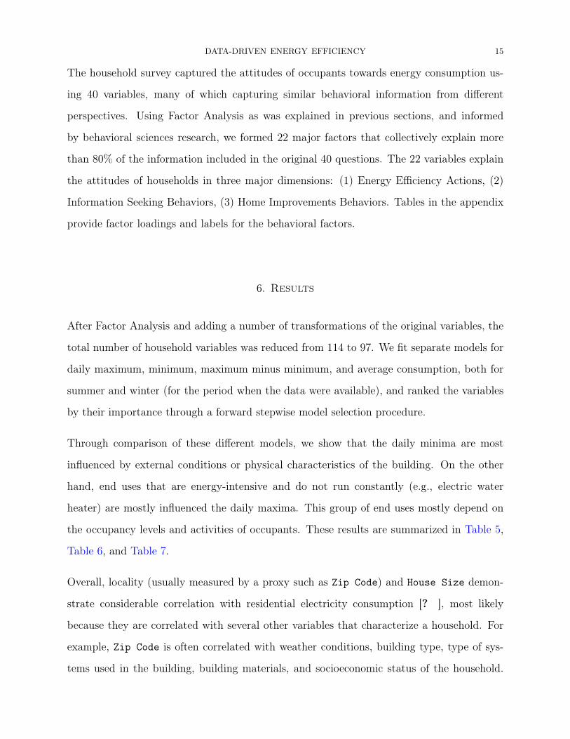
6. Results
After Factor Analysis and adding a number of transformations of the original variables, the
total number of household variables was reduced from 114 to 97. We fit separate models for
daily maximum, minimum, maximum minus minimum, and average consumption, both for
summer and winter (for the period when the data were available), and ranked the variables
by their importance through a forward stepwise model selection procedure.
Through comparison of these different models, we show that the daily minima are most
influenced by external conditions or physical characteristics of the building. On the other
hand, end uses that are energy-intensive and do not run constantly (e.g., electric water
heater) are mostly influenced the daily maxima. This group of end uses mostly depend on
the occupancy levels and activities of occupants. These results are summarized in Table 5,
Table 6, and Table 7.
Overall, locality (usually measured by a proxy such as Zip Code) and House Size demon-
strate considerable correlation with residential electricity consumption [? ], most likely
because they are correlated with several other variables that characterize a household. For
example, Zip Code is often correlated with weather conditions, building type, type of sys-
tems used in the building, building materials, and socioeconomic status of the household.

DATA-DRIVEN ENERGY EFFICIENCY 16
On the other hand, House Size is often correlated with affluence, socioeconomic status,
number of residents, and appliance stock. We fitted separate models with and without Zip
Code (using the first two digits of zip code to avoid over-fitting) and House Size to (a)
study the impact of locality and house size on electricity consumption, and (b) identify the
variables that are obscured by zip code and house size through a comparison of the models
with and without these two variables.
6.1. The Effect of External Determinants on Residential Electricity Consump-
tion. As it is expected, when included in the model, Zip Code is a significant determinant of
household electricity consumption, contributing by up to 46% to the variability in consump-
tion. However, once Zip Code is removed from the models, underlying drivers of electricity
consumption such as Cooling Degree Days are highlighted. This is expected because Zip
Code is a proxy for climate and weather, and hence obscures cooling degree days when it is
present in the model.
Cooling Degree Day(CDD) is the dominant factor in the summer, explaining 38% of the vari-
ability in total electricity consumption. On the other hand, Heating Degree Day (HDD) is
not a significant factor, even in the winter model. We offer an explanation for this observation
in subsection 6.2.

DA
TA
-DR
IVE
NE
NE
RG
YE
FFIC
IEN
CY
17
Table 5. Summary of the most important factors explaining different aspects of residential electricity consumption. (F:full model; P: partial model (excluding Zip Code and Floor Area))
Variable Min Max Max-Min Average
Summer Winter Summer Winter Summer Winter Summer Winter
F P F P F P F P F P F P F P F PAve. of CDD 26% 31% 27% 38%Climate Zone 2% 3%Zip Code 12% 12% 39% 26% 37% 25% 46% 17%House Size 2% 21% 11% 2% 9% 12% 23%Type of bldg 12% 2%Ownership of elec.water heater 4% 4% 11% 2% 6% 5% 12% 2% 5%
Ownership of elec.clothes dryer 2% 2% 3% 3% 2% 4%
Nb of spas/pools 2% 2% 2%Nb of freezers 3% 2%Nb of refrig’s 7% 7% 7% 7% 3% 4% 4% 3% 2% 2% 3% 2% 3% 4% 6% 6%Nb of entert’t devicesExcept TV’s 3% 2% 4% 2%
Total nb of occup’ts 8%Total nb of occup’ts(sq. rt) 2% 2% 2% 4% 2% 3% 7% 4% 2% 2%
Pet ownership 2% 2% 2% 4% 3% 2% 3%Purchasing E-Star Appl’s 2% 2% 2% 3% 2%Energy Conserv’n w.r.t.Elec. Heater Usage 2% 2% 2% 2%
Turning lights offwhen not in use 19% 13% 20%
Motivated to reduce coumspt’nto address Global Warm. 2% 2% 3%
Summer model: total number of variables: 93; R2adj=0.52
Winter model: total number of variables: 82; R2adj=0.48

DA
TA
-DR
IVE
NE
NE
RG
YE
FFIC
IEN
CY
18
Table 6. Summary of the model coefficients of the most important factors explaining different aspects of residentialelectricity consumption for minimum and maximum consumption models. (F: full model; P: partial model (excluding ZipCode and Floor Area)
Variable Min Max
Summer Winter Summer Winter
F P F P F P F PAve. of CDD 0.005 0.001 0.052Climate Zone -0.35 to +0.12
(ave: -0.03)Zip Code -0.30 to +1.66 -0.27 to 1.13 -1.47 to +3.51 -2.64 to +2.50
(ave: 0.26) (ave: 0.13) (ave: 0.011) (ave: 0.03)House Size -0.28 to +0.75 -0.04 to +0.13 -0.35 to +3.35 -1.40 to +1.73
(ave: 0.04) (ave: 0.38) (ave: 0.74) (ave: 0.74)Type of bldg
Ownership of elec.water heater 0.670 1.009
Ownership of elec.clothes dryer 0.344 0.396
Nb of spas/poolsNb of freezers 0.061 0.234Nb of refrig’s 0.308 0.305 0.106 0.239 0.941 1.08 0.941Nb of entert’t devicesExcept TV’s 0.020 0.013 0.019 0.026
Total nb of occup’ts -0.05Total nb of occup’ts(sq. rt) 0.987 1.14 0.792
Pet ownership 0.036 0.042 0.021 0.029 0.058 0.148Purchasing E-Star Appl’s 0.008 0.013 0.013 0.015Energy Conserv’n w.r.t.Elec. Heater Usage -0.026 -0.015 -0.017
Turning lights off 0.046when not in use
Motivated to reduce coumspt’nto address Global Warm.
Summer model: total number of variables: 93; R2adj=0.52
Winter model: total number of variables: 82; R2adj=0.48
DA
TA
-DR
IVE
NE
NE
RG
YE
FFIC
IEN
CY
19
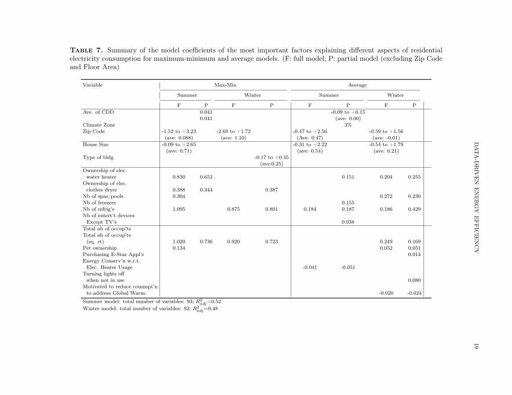
Table 7. Summary of the model coefficients of the most important factors explaining different aspects of residentialelectricity consumption for maximum-minimum and average models. (F: full model; P: partial model (excluding Zip Codeand Floor Area)
Variable Max-Min Average
Summer Winter Summer Winter
F P F P F P F PAve. of CDD 0.041 -0.09 to +0.15
0.041 (ave: 0.00)Climate Zone 3%Zip Code -1.52 to +3.23 -2.69 to +1.72 -0.47 to +2.56 -0.59 to +1.56
(ave: 0.088) (ave: 1.10) (Ave: 0.47) (ave: -0.01)House Size -0.09 to +2.65 -0.31 to +2.22 -0.54 to +1.79
(ave: 0.71) (ave: 0.54) (ave: 0.21)Type of bldg -0.17 to +0.45
(ave:0.25)Ownership of elec.water heater 0.830 0.652 0.151 0.204 0.255
Ownership of elec.clothes dryer 0.388 0.344 0.387
Nb of spas/pools 0.304 0.272 0.230Nb of freezers 0.155Nb of refrig’s 1.095 0.875 0.801 0.184 0.187 0.186 0.429Nb of entert’t devicesExcept TV’s 0.038
Total nb of occup’tsTotal nb of occup’ts(sq. rt) 1.020 0.736 0.920 0.723 0.249 0.169
Pet ownership 0.134 0.052 0.051Purchasing E-Star Appl’s 0.014Energy Conserv’n w.r.t.Elec. Heater Usage -0.041 -0.051
Turning lights offwhen not in use 0.080
Motivated to reduce coumspt’nto address Global Warm. -0.020 -0.024
Summer model: total number of variables: 93; R2adj=0.52
Winter model: total number of variables: 82; R2adj=0.48

DATA-DRIVEN ENERGY EFFICIENCY 20
6.2. The Effect of Physical Characteristics of the Dwelling. Type of building and
house size are the most important factors among building characteristics in our models, while
house age and ownership status do not show significant impact on electricity consumption
in our sample. Other variables such as insulation level and installation of energy-efficient
lighting fixtures show correlation with reduced electricity use when analyzed individually;
however, in the full model with other variables they do not show a significant impact. The
following sections explain these results in more detail.
6.2.1. Type of building. Type of Building is most significant in the winter daily maximum
model where heating load dominates. In the winter, households who live in multifamily
apartments have the lowest daily maximum consumption (per household), followed by town
houses; finally, detached (free-standing) houses have the highest daily maximum consumption
in the winter. Similar results are reported by Guerra Santin et al. [25] and Haas [26].
6.2.2. House size. Based on the results of our models, the effect of House Size is more
pronounced in the winter models: while House Size explains 21% of winter minimum load,
it only explains 2% of the minimum load during summer. The large difference between House
Size’s impact on summer and winter load shows that heating load is more dependent on
the size of the house, compared to cooling load that has an intermittent load nature: a
larger house not only requires more heating energy to warm up, but also has higher heat loss
through larger building envelope areas.
Inverse to daily minimum and average loads, the effect of House Size on daily maximum and
maximum-minimum is more pronounced during the summer. Again, this can be explained
by the inherent relationship of house size and space conditioning load. In the summer, when
the dominant space conditioning load is cooling load, house size is a major contributor to
daily maximum load, because cooling load (air conditioning electricity consumption) is often
active only during a few hours of a day, peaking at certain times.
DATA-DRIVEN ENERGY EFFICIENCY 21
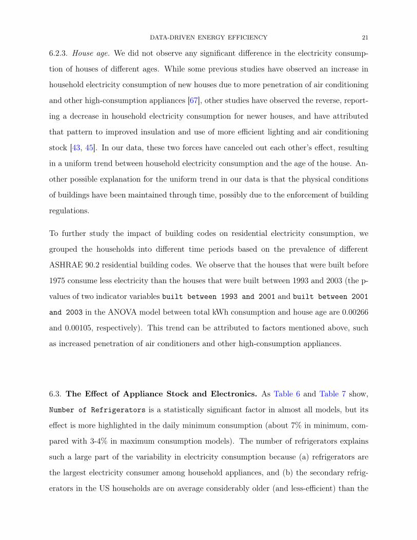
6.2.3. House age. We did not observe any significant difference in the electricity consump-
tion of houses of different ages. While some previous studies have observed an increase in
household electricity consumption of new houses due to more penetration of air conditioning
and other high-consumption appliances [67], other studies have observed the reverse, report-
ing a decrease in household electricity consumption for newer houses, and have attributed
that pattern to improved insulation and use of more efficient lighting and air conditioning
stock [43, 45]. In our data, these two forces have canceled out each other’s effect, resulting
in a uniform trend between household electricity consumption and the age of the house. An-
other possible explanation for the uniform trend in our data is that the physical conditions
of buildings have been maintained through time, possibly due to the enforcement of building
regulations.
To further study the impact of building codes on residential electricity consumption, we
grouped the households into different time periods based on the prevalence of different
ASHRAE 90.2 residential building codes. We observe that the houses that were built before
1975 consume less electricity than the houses that were built between 1993 and 2003 (the p-
values of two indicator variables built between 1993 and 2001 and built between 2001
and 2003 in the ANOVA model between total kWh consumption and house age are 0.00266
and 0.00105, respectively). This trend can be attributed to factors mentioned above, such
as increased penetration of air conditioners and other high-consumption appliances.
6.3. The Effect of Appliance Stock and Electronics. As Table 6 and Table 7 show,
Number of Refrigerators is a statistically significant factor in almost all models, but its
effect is more highlighted in the daily minimum consumption (about 7% in minimum, com-
pared with 3-4% in maximum consumption models). The number of refrigerators explains
such a large part of the variability in electricity consumption because (a) refrigerators are
the largest electricity consumer among household appliances, and (b) the secondary refrig-
erators in the US households are on average considerably older (and less-efficient) than the
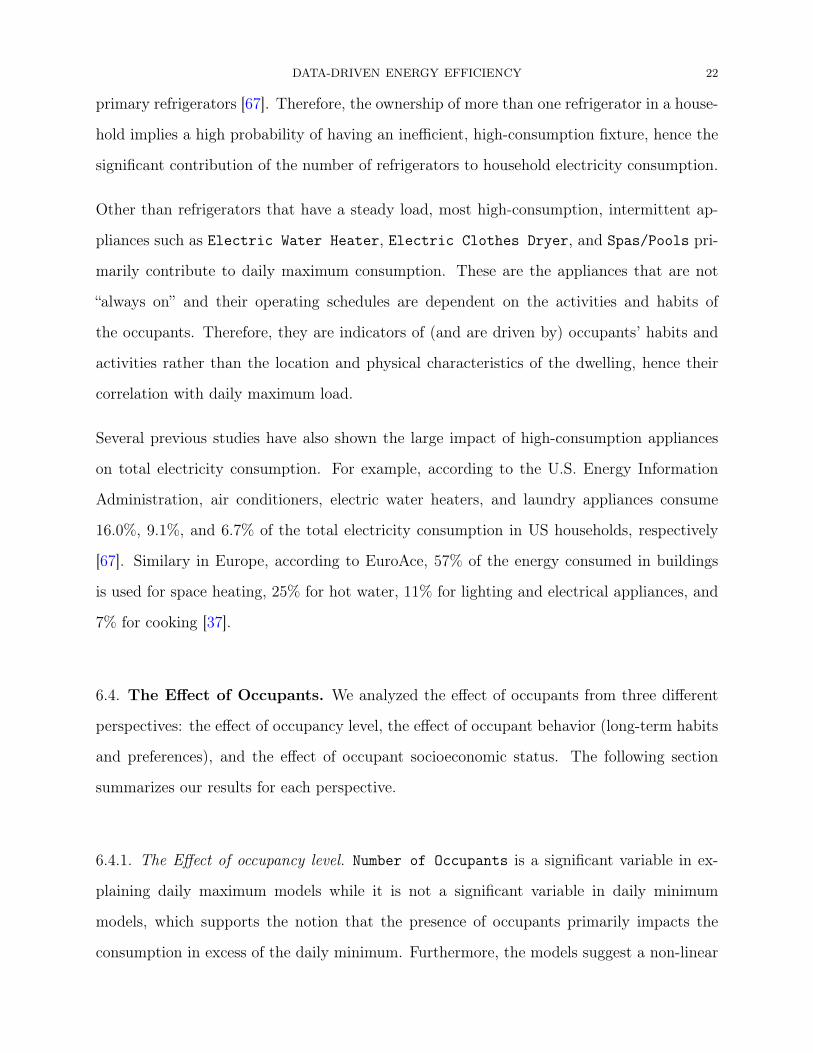
DATA-DRIVEN ENERGY EFFICIENCY 22
primary refrigerators [67]. Therefore, the ownership of more than one refrigerator in a house-
hold implies a high probability of having an inefficient, high-consumption fixture, hence the
significant contribution of the number of refrigerators to household electricity consumption.
Other than refrigerators that have a steady load, most high-consumption, intermittent ap-
pliances such as Electric Water Heater, Electric Clothes Dryer, and Spas/Pools pri-
marily contribute to daily maximum consumption. These are the appliances that are not
“always on” and their operating schedules are dependent on the activities and habits of
the occupants. Therefore, they are indicators of (and are driven by) occupants’ habits and
activities rather than the location and physical characteristics of the dwelling, hence their
correlation with daily maximum load.
Several previous studies have also shown the large impact of high-consumption appliances
on total electricity consumption. For example, according to the U.S. Energy Information
Administration, air conditioners, electric water heaters, and laundry appliances consume
16.0%, 9.1%, and 6.7% of the total electricity consumption in US households, respectively
[67]. Similary in Europe, according to EuroAce, 57% of the energy consumed in buildings
is used for space heating, 25% for hot water, 11% for lighting and electrical appliances, and
7% for cooking [37].
6.4. The Effect of Occupants. We analyzed the effect of occupants from three different
perspectives: the effect of occupancy level, the effect of occupant behavior (long-term habits
and preferences), and the effect of occupant socioeconomic status. The following section
summarizes our results for each perspective.
6.4.1. The Effect of occupancy level. Number of Occupants is a significant variable in ex-
plaining daily maximum models while it is not a significant variable in daily minimum
models, which supports the notion that the presence of occupants primarily impacts the
consumption in excess of the daily minimum. Furthermore, the models suggest a non-linear
DATA-DRIVEN ENERGY EFFICIENCY 23
relationship between household electricity consumption and the number of occupants, select-
ing the Square Root of Number of Occupants over the Number of Occupants. In other
words, our model verifies that when the number of occupants double, electricity consumption
increases at a slower rate (1.4 in our data), leading to the conclusion that larger households
have higher aggregate electricity consumption but lower per capita consumption. A similar
concave non-linear relationship between number of occupants and electricity consumption
has been reported by [7, 30, 70].
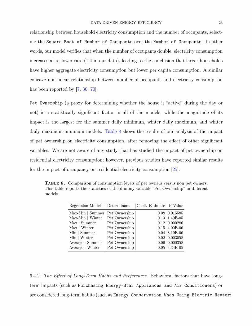
Pet Ownership (a proxy for determining whether the house is “active” during the day or
not) is a statistically significant factor in all of the models, while the magnitude of its
impact is the largest for the summer daily minimum, winter daily maximum, and winter
daily maximum-minimum models. Table 8 shows the results of our analysis of the impact
of pet ownership on electricity consumption, after removing the effect of other significant
variables. We are not aware of any study that has studied the impact of pet ownership on
residential electricity consumption; however, previous studies have reported similar results
for the impact of occupancy on residential electricity consumption [25].
Table 8. Comparison of consumption levels of pet owners versus non pet owners.This table reports the statistics of the dummy variable “Pet Ownership” in differentmodels.
Regression Model Determinant Coeff. Estimate P-Value
Max-Min | Summer Pet Ownership 0.08 0.015585Max-Min | Winter Pet Ownership 0.13 1.49E-05Max | Summer Pet Ownership 0.12 0.000286Max | Winter Pet Ownership 0.15 4.00E-06Min | Summer Pet Ownership 0.04 8.19E-06Min | Winter Pet Ownership 0.02 0.003058Average | Summer Pet Ownership 0.06 0.000358Average | Winter Pet Ownership 0.05 3.34E-05
6.4.2. The Effect of Long-Term Habits and Preferences. Behavioral factors that have long-
term impacts (such as Purchasing Energy-Star Appliances and Air Conditioners) or
are considered long-term habits (such as Energy Conservation When Using Electric Heater;

DATA-DRIVEN ENERGY EFFICIENCY 24
i.e., adjusting thermostat settings moderately and according to occupancy) are significant
explanatory variables for daily minimum consumption.
As Table 6 (variable coefficient estimates) shows, in the daily minimummodel, the behavior of
Purchasing Energy-Star Appliances and Air Conditioners has a positive coefficient.
This suggests that, in our study sample, contrary to common belief, households that have
expressed motivation to buy energy-efficient appliances and air conditioners have higher levels
of daily minimum consumption, after adjusting for all other variables. Similar observations
have been reported by several previous researchers, leading Sütterlin et al. [61] to declare that
“the green purchaser is not necessarily the green consumer”. Some researchers have attributed
this behavior to the “rebound effect” where an increase in the efficiency of appliances results
in increased use of them [1, 9].
Another long-term habit is Turning Off Lights When Not in Use, which is significant for
most winter models. However, the variable that represents the habit of Turning Lights Off
When Not In Use manifests a significant geographical pattern, as it becomes insignificant
when Zip Code is included in the model. While turning unnecessary lights off reduces con-
sumption, the effect of its associated variable is augmented in our sample by the geographical
distribution of the households on the two coasts that have declared environment-conscious
behavior, and at the same time benefit from milder climate throughout the year. Therefore,
further data are needed to quantify the individual effect of energy-conscious behavior of
turning off unnecessary lights.
6.4.3. Effect of Income Level. We did not observe any statistically significant correlation
between Income Level and electricity consumption. In our sample, more affluent house-
holds tend to have lower daily maximum consumption values in the summer compared to
less-affluent households, because they have more energy-efficient appliances on average (see
Figure 2). This is significant because the most important determinants of the summer daily

DATA-DRIVEN ENERGY EFFICIENCY 25
maximum model are (model coefficients in parenthesis): cooling degree days (0.052), owner-
ship of electric water heater (0.670), ownership of electric clothes dryer (0.344), number of
occupants (0.984), and climate zone (five categorical variables ranging from -0.353 to 0122).
Furthermore, since all participants of the study are well-educated and work in a high-tech
company, one can conclude that once the consumers pass a certain level of education and
awareness of energy efficiency matters, the more affluent they are, the lower their daily maxi-
mum consumption is likely to be, mainly because of improved efficiency of high-consumption
appliances.
The relationship between household income and energy consumption has been the subject
of extensive research. While a large number of studies have concluded that energy con-
sumption increases monotonically with income [10, 12, 20, 69], a number of studies have
reported observing an inverted U-path comparing energy consumption and household in-
come. At the same time, the effect of income on household electricity consumption has
been shown to be mediated by ownership of appliances: since electricity cost makes up a
small percent of households’ expenditure, economic factors such as price of electricity and
income of the household impact the consumption through affecting the stock (quantity and
quality) of appliances rather than having a direct effect (Sudarshan [59] offers more details
on this hypothesis and cites previous works that confirm this hypothesis [16, 50, 54]). This
hypothesis is in agreement with the inverse U-path observation: in the lower-income segment
of the inverted U-path which is the monotonically-increasing part, households acquire more
energy-intensive appliances as the level of income increases. Then, once the income passes
a certain level, in the decreasing segment of the U-path, households purchase more efficient
appliances as their level of income increases [18, 21, 40, 42]. Our data captures the latter
part of the inverted U-path when the energy consumption decreases as the level of income
increases, since we have data from well-educated and middle to upper class households.
The plots of selected stepwise models are included in the appendix to illustrate how a few
important factors explain the variability in residential electricity consumption.

DATA-DRIVEN ENERGY EFFICIENCY 26
Figure 2. Daily maximum consumption slightly reduces with increase in income(not a statistically significant trend). The kWh consumption is not adjusted for anyother effect to enable a direct comparison of kWh consumption versus income.
6.5. Results of Individual ANOVA Models. Other than age, size, and type, other
physical characteristics of the building were not selected by our stepwise model. However,
several of those variables have significant correlation with electricity consumption, but were
not selected for the multivariate model because of their correlation with other variables in
the model. In other words, once a variable is added to the model, it “explains away” the
effect of other variables with which it is correlated. Because of the importance of several
physical characteristics of buildings for policy making and planning for energy efficiency, we
summarize the results of the individual models in this section.
6.5.1. Ownership Status. Our data do not show statistically significant difference in elec-
tricity consumption between rented and owned houses, contrary to several previous studies
which showed that energy consumption is higher in rented houses, especially when the energy
bill is included in the rent as a lump sum [25].
DATA-DRIVEN ENERGY EFFICIENCY 27
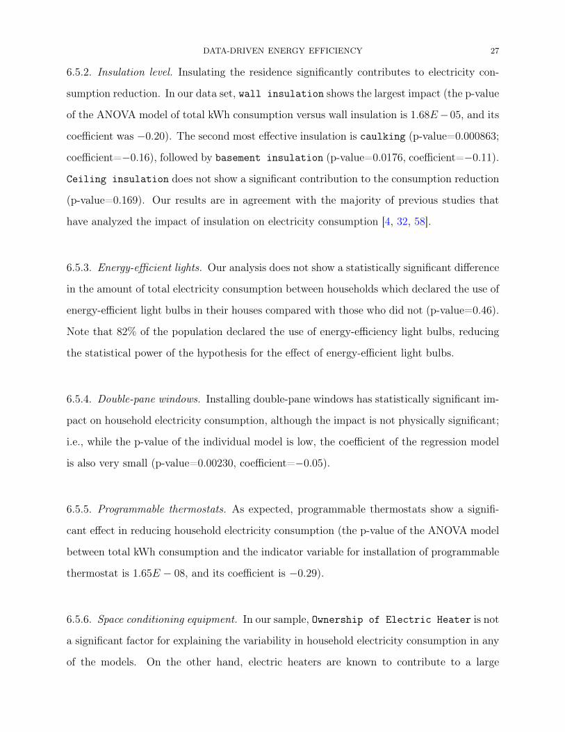
6.5.2. Insulation level. Insulating the residence significantly contributes to electricity con-
sumption reduction. In our data set, wall insulation shows the largest impact (the p-value
of the ANOVA model of total kWh consumption versus wall insulation is 1.68E−05, and its
coefficient was −0.20). The second most effective insulation is caulking (p-value=0.000863;
coefficient=−0.16), followed by basement insulation (p-value=0.0176, coefficient=−0.11).
Ceiling insulation does not show a significant contribution to the consumption reduction
(p-value=0.169). Our results are in agreement with the majority of previous studies that
have analyzed the impact of insulation on electricity consumption [4, 32, 58].
6.5.3. Energy-efficient lights. Our analysis does not show a statistically significant difference
in the amount of total electricity consumption between households which declared the use of
energy-efficient light bulbs in their houses compared with those who did not (p-value=0.46).
Note that 82% of the population declared the use of energy-efficiency light bulbs, reducing
the statistical power of the hypothesis for the effect of energy-efficient light bulbs.
6.5.4. Double-pane windows. Installing double-pane windows has statistically significant im-
pact on household electricity consumption, although the impact is not physically significant;
i.e., while the p-value of the individual model is low, the coefficient of the regression model
is also very small (p-value=0.00230, coefficient=−0.05).
6.5.5. Programmable thermostats. As expected, programmable thermostats show a signifi-
cant effect in reducing household electricity consumption (the p-value of the ANOVA model
between total kWh consumption and the indicator variable for installation of programmable
thermostat is 1.65E − 08, and its coefficient is −0.29).
6.5.6. Space conditioning equipment. In our sample, Ownership of Electric Heater is not
a significant factor for explaining the variability in household electricity consumption in any
of the models. On the other hand, electric heaters are known to contribute to a large

DATA-DRIVEN ENERGY EFFICIENCY 28
portion of household electricity consumption. For example, in the US in 2001, heating, ven-
tilation, and air conditioning (HVAC) accounted for about 30% of total residential electricity
consumption; during that period, electric heaters alone consumed 10% of total household
electricity consumption (which is significant since only 29% of US households used electricity
as the main heating fuel for their houses in 2001) [67]. This discrepancy in our results with
those of previous studies is partly because only 19% of the population indicated that their
central space heater uses electricity, compared with the national average of 29%. On the
other hand, some variables that are related to heating load, such as House Size and Energy
Conservation When Using Electric Heater, are capturing the effect of heating during
the winter.
Number of Air Conditioners is not a statistically significant variable in our models; in-
stead, Cooling Degree Days (CDD) is capturing the effect of air conditioners: CDD ex-
plains 26%, 31%, 27%, 38% of the total variability in residential electricity in the summer
for minimum, maximum, maximum-minimum, and average electricity consumption, respec-
tively. This pattern is in line with the results of previous research that shows that 31% of
total household electricity is consumed by electric air conditioning systems, making thm the
largest consumers of household electricity [67].
7. Conclusions
The electricity consumption of US households has been increasing in the past decades, and
is projected to continue its upward trend [68]. Based on a sound understanding of the
factors that drive household electricity consumption, policy measures can be designed and
implemented to effectively reduce consumption. These measures can target macro-level
factors such as technological developments, regulations, cultural and social norms; or, they
can target micro-level factors such as individual decision-making of households for energy
efficiency and conservation [22, 49]. Summarizing our findings, we showed that:

DATA-DRIVEN ENERGY EFFICIENCY 29
(a) Factors that influence residential electricity consumption can be categorized into four
major groups: external conditions (e.g., location and weather), physical characteristics
of dwelling, appliance and electronics stock, and occupants.
(b) Each of the four categories above, on average, has a different time span and effort level for
modification; while location, weather, and occupancy are outside the scope of influence
for modification, physical characteristics of the building, appliance stock, and occupant
behavior factors can be modified in long-term, medium-term, and short-term investment
spans, respectively. Accordingly, the persistence of the modification effect is generally
proportional to the level of effort and investment that was allocated to it.
(c) Daily minimum and daily maximum consumption are explained by different sets of ex-
planatory factors. Daily minimum has a lower variation level compared with daily max-
imum, and is best explained by factors that are steady through time, such as weather
(Degree Days), location (Zip Code), House Size, and Number of Refrigerators. On
the other hand, daily maximum is best explained by large and intermittent loads such
as Electric Water Heater and Air Conditioners.
(d) Using our model, we were able to explain 55-65% of the variability in electricity con-
sumption, as measured by the R2 of the regression model. This is comparable with
most studies in the past. Using variable transformations and other machine learning
techniques [39], we were able to achieve R2 values of above 70%. However, the linear
model is still preferred because it faciliates interpretation because its coefficients have
physical significance (i.e., the coefficients of different variables can be compared with
each other to estimate their physical impact on electricity consumption). Furtheremore,
we deliberately did not use variables such as Zip Code or the households’ estimate of
their electricity bill (both available from the survey) that improve the R2 of the fit, but
add little explanatory significance to the results of the model.
(e) Overall, weather and physical characteristics of the building illustrate more influence
on residential electricity consumption compared to other categories such as occupant
behavior. These results are comparable with the results reported by Guerra Santin
DATA-DRIVEN ENERGY EFFICIENCY 30
et al. [25] who showed that building characteristics determine 42% of the variability in
residential electricity consumption, whereas occupant behavior explains 4.2% (see 5 for
our results). Within the physical characteristics of the building, floor area, type of
building, and use of electric water heater contributed the most to consumption,
whereas within the appliance stock, number of refrigerators was the most important
factor. Finally, pet ownership (which can be considered a proxy for the percent of time
that the house is active) was a significant factor in explaining variation in electricity
consumption.
8. Policy Implications
Based on the results of our models, we highly recommend policies and regulations aimed at
improving the thermal performance of buildings, including both improvements to the insu-
lation level of the dwelling and improving the efficiency of the stock of air conditioning and
electric heaters. Since certain end uses such as space heating are more prone to rebound
effects [12], we strongly recommend provisions for regular home energy audits in codes and
regulations [32]. Furthermore, we recommend policies and regulations aimed at improving
the efficiency of the appliance stock. Certain end uses such as refrigerators illustrate great
potential for consumption reduction. Refrigerators consumed 14% of total electricity deliv-
ered to U.S. homes in 2001, only second to air conditioners who consumed 15% [67]. This
situation is exacerbated because the second refrigerator in the US households is on average
considerably older (and less efficient) than the primary refrigerator [67]. This suggests that
many US households do not discard their old, inefficient refrigerator when they purchase a
new one. Therefore, policies and programs that encourage the purchase of energy-efficient
refrigerators must also devise provisions for buying back the old refrigerators or make the
financial incentive contingent on households returning the old refrigerators.
Other kitchen and laundry appliances are also significant contributors to household electric-
ity consumption, and collectively are responsible for 17% (excluding refrigerators) of total

DATA-DRIVEN ENERGY EFFICIENCY 31
residential electricity consumption in the U.S. [67]. Most high-consumption, intermittent
appliances such as Electric Water Heater, Electric Clothes Dryer, and Spas/Pools
demand high volume and intermittent electric loads, hence are attractive targets for both
consumption reduction and load shifting programs and policies. Since these end uses are
primarily driven by occupants’ habits and activities rather than the location and physical
characteristics of the dwelling, policies that target reducing electricity consumption of these
high-consumption, intermittent appliances must be focused primarily on behavioral modifi-
cation. For example, educational campaigns encouraging households to use larger loads of
laundry, to lower the temperature of their electric water heaters, or to shift their laundry
time to a more appropriate time in the day can be effective in this regard.
On the other hand, contrary to several previous studies, we did not observe any statistically-
significant correlation between income level and electricity consumption. The slight trend
observed was inverse of previous observations [10, 12, 20, 69]: as Figure 2 shows, more
affluent households in our sample tend to have lower values of peak consumption compared
to less-affluent households. This observation, combined with previous observations on the
ineffectiveness of tax credits in certain populations [51] suggest that tax credits and financial
rewards need to be supported by additional policies to be effective [12].
In terms of the impact of behavioral factors, our study confirmed the views of Cramer [15]
that residential electricity consumption is primarily determined through the way households
use electricity, rather than the way they value energy efficiency. On the other hand, some
energy-saving values impact efficiency through certain longer-term “habits” such as purchas-
ing energy-star appliances. These are also the group of habits that are most influenced
by changes in price of electricity [20]. These observations suggest that behavior modifica-
tion programs can be more effective when supported by monetary and regulatory policies.
Ultimately, the factors that drive consumption can vary significantly from one population
to another. This diversity is even more pronounced when the behavioral determinants of
electricity consumption are studied. Our model is a first step to disaggregate the impact

DATA-DRIVEN ENERGY EFFICIENCY 32
of structural determinants from that of behavioral determinants using high-resolution con-
sumption data. However, we observed considerable diversity among the results of previous
works and our model. Therefore, we strongly recommend that future energy-efficiency pro-
gramming efforts collect specific data about target population and use population-specific
data to build models.
9. Contribution
This paper offers several contributions to the body of knowledge in residential electricity
consumption modeling. First, it formalizes a methodology to analyze large data sets of resi-
dential electricity consumption and household information, by using statistical methods such
as Factor Analysis and stepwise regression, and the application of building sciences domain
knowledge. Furthermore, by distinguishing the daily minimum load versus maximum load,
the model offers a novel method to disaggregate the impact of long-term factors versus that
of short-term factors. While most available studies use total consumption to explain residen-
tial electricity usage, using our models we show that different aspects of energy usage such
as daily minimum have different patterns and are explained by different characteristics of
the household (see Figure ?? and Table 5). Furthermore, we show that disaggregating elec-
tricity load allows for identification of the individual impact of factors that drive electricity
consumption. For example, some factors such as ownership of electric clothes dryers only
contribute to daily maximum consumption, while some other factors such as considering en-
ergy conservation when using electric heater only contribute to daily minimum consumption.
This work presents a new method for adjusting for the effect of the floor area of the residence
on its electricity consumption: instead of the common practice of applying a global factor
of the inverse of the floor area, this paper suggests a more realistic model in which only the
impact of those end uses which are correlated with floor area are augmented. Finally, by
applying model selection techniques (i.e., forward stepwise regression), this work identifies a
set of variables that are most important in explaining the variability in residential electricity
consumption. This reduced set of variables (Table 5) can be used in the experimental design

DATA-DRIVEN ENERGY EFFICIENCY 33
for future studies, where the number of questions asked in a questionnaire or the amount of
data that can be collected about subjects is limited and should be reduced to the smallest
number of questions that explain an adequate amount of variability in electricity consump-
tion. Ultimately, this paper illustrates how the results of residential electricity consumption
models can be used by policy makers and program managers of energy efficiency programs in
utility companies. Especially, the distinction between short-term, medium-term, and long-
term factors that impact residential electricity consumption can be used by energy-efficiency
planners to inform strategic planning and management of demand-side energy efficiency pro-
grams. Moreover, the paper presents the implications of the model results for building and
appliance codes and regulations and behavioral modification campaigns. Future researchers
in this field can also use the methods presented in this work to analyze large data sets of
smart meter data and household information more efficiently and effectively.
10. Future Work
More data are needed to validate some of the findings of this paper. Specifically, household
data from a more heterogeneous sample over a larger period of time are needed for validating
the generality of these results. The use of self-reports to measure behavior may have intro-
duced some bias in the data, called “social desirability” bias [53]. However, since the purpose
of this study was to explain the variability in electricity consumption, and furthermore the
households in our study were all from middle and upper social class, we assume that the
bias in responses were uniform over the respondents and therefore the results of the model
explain the variability in electricity consumption with a reasonable accuracy.
In this paper, we examined energy consumption and its features such as daily maximum and
minimum consumption, and explained their variability using household data. A potential
follow-up to this study is to develop a metric for quantifying energy efficiency of the house-
holds, and compare households using that metric instead of their consumption data. Such

DATA-DRIVEN ENERGY EFFICIENCY 34
metric needs to be defined in a way that recognizes the inherent differences among different
groups of households and at the same time enables comparison across those different groups.
11. Acknowledgments
The majority of this work was funded through Advanced Research Projects Agency-Energy
(ARPA-E) grant to Stanford University. Ram Rajagopal was supported by the Powell Foun-
dation Fellowship. The authors would like to thank Dr. June Flora at H-STAR Institute at
Stanford University for helpful inputs and comments during this study.
References
[1] Abrahamse, W., L. Steg, C. Vlek, and T. Rothengatter (2005, September). A review of interven-
tion studies aimed at household energy conservation. Journal of Environmental Psychology 25 (3),
273–291.
[2] Aigner, D., C. Sorooshian, and P. Kerwin (1984). Conditional Demand Analysis for Estimating
Residential End-Use Load Profiles. The Energy Journal 5 (4), 81–97.
[3] Alcott, B. (2008, February). The sufficiency strategy: Would rich-world frugality lower environ-
mental impact? Ecological Economics 64 (4), 770–786.
[4] Assimakopoulos, V. (2000). Residential energy demand modelling in developing regions The use
of multivariate statistical techniques. Energy Policy , 57–63.
[5] Aydinalp, M., V. Ugursal, and a.S. Fung (2003, March). Modelling of residential energy con-
sumption at the national level. International Journal of Energy Research 27 (4), 441–453.
[6] Baltagi, B. (2002, August). Comparison of forecast performance for homogeneous, heterogeneous
and shrinkage estimators Some empirical evidence from US electricity and natural-gas consumption.
Economics Letters 76 (3), 375–382.
[7] Barnes, D. F., K. Krutilla, and W. Hyde (2004). The Urban Household Energy Transition.
Technical Report March, Resources for the Future.
[8] Bartels, R. and D. Fiebig (1998). Metering and modelling residential end use electricity load
curves. Forecasting 15 (6), 415–426.

DATA-DRIVEN ENERGY EFFICIENCY 35
[9] Beerepoot, M. (2007). Energy policy instruments and technical change in the residential building
sector. Alblasserdam, The Netherlands: Haveka.
[10] Biesiot, W. and K. J. Noorman (1999). Energy requirements of household consumption : a
case study of The Netherlands. Ecological Economics 28, 367 – 383.
[11] Caves, D. W., J. a. Herriges, K. E. Train, and R. J. Windle (1987, August). A Bayesian
Approach to Combining Conditional Demand and Engineering Models of Electricity Usage. The
Review of Economics and Statistics 69 (3), 438.
[12] Cayla, J.-M., N. Maizi, and C. Marchand (2011, October). The role of income in energy
consumption behaviour: Evidence from French households data. Energy Policy 39 (12), 7874–
7883.
[13] Cherfas, J. (1991). Skeptics and Visionaries Examine Energy Saving. Science 251 (4990),
154–156.
[14] Courrieu, P. and A. Rey (2011). Missing data imputation and corrected statistics for large-scale
behavioral databases. Behavior research methods 43 (2), 310–30.
[15] Cramer, J. C. (1985). Social and engineering determinants and their equity implications in
residential electricity use. Energy 10 (12), 1283–1291.
[16] Dubin, J. A. and D. Mcfadden (1984). An Econometric Analysis of Residential Electric Appli-
ance Holdings and Consumption. Society 52 (2), 345–362.
[17] Ehrhardt-martinez, K. and K. A. Donnelly (2010). Advanced Metering Initiatives and Residen-
tial Feedback Programs : A Meta-Review for Household Electricity-Saving Opportunities. Energy .
[18] Elias, R. J. and D. G. Victor (2005). Energy Transitions in Developing Countries - A Review
of Concepts and Literature, Working Paper 40.
[19] Everitt, B. and T. Hothorn (2011). Exploratory Factor Analysis. In An Introduction to Applied
Multivariate Analysis with R, Chapter 05, pp. 135–161. New York, NY: Springer New York.
[20] Filippini, M. (2011). Short- and long-run time-of-use price elasticities in Swiss residential
electricity demand. Energy Policy 39 (10), 5811–5817.
[21] Foster, V., J.-p. Tre, and Q. Wodon (2000). Energy consumption and income : An inverted-U
at the household level ?
[22] Gatersleben, B. and C. Vlek (1997). Household Consumption, Quality of Life, and Environmen-
tal Impact: A Psycholoigcal Perspective and Empirical Study. In K. Noorman and T. Uiterkamp

DATA-DRIVEN ENERGY EFFICIENCY 36
(Eds.), Green Households: Domestic Consumers, The Environment and Sustainability, Chapter 7,
pp. 1997. Earthscan Publications Ltd.
[23] Gelman, A. and J. Hill (2007). Missing data imputation. Behavior research methods 43 (2),
310–30.
[24] Goldfarb, D. L. and R. Huss (1988). Building Utility Scenarios for an Electric. Long Range
Planning 21 (2), 78–85.
[25] Guerra Santin, O., L. Itard, and H. Visscher (2009, November). The effect of occupancy and
building characteristics on energy use for space and water heating in Dutch residential stock.
Energy and Buildings 41 (11), 1223–1232.
[26] Haas, R. (1997). Energy efficiency indicators in the residential sector What do we know and
what has to be ensured? Distribution 25, 789–802.
[27] Haas, R. and L. Schipper (1998, March). Residential energy demand in OECD-countries and
the role of irreversible efficiency improvements. Energy Economics 20 (4), 421–442.
[28] Halvorsen, R. (1975). Residential Demand for Electric Energy. The Review of Economics and
Statistics 57 (1), 12–18.
[29] Hastie, T. and R. Tibshirani (2011). The Elements of Statistical Learning. Springer.
[30] Heltberg, R. (2005). Factors determining household fuel choice in Guatemala. Environment
and Development Economics 10 (3), 337–361.
[31] Hirst, E. (1978). A model of residential energy use. Simulation 30 (3), 69–74.
[32] Hirst, E. and R. Goeltz (1985). Comparison of Actual Energy Savings with Audit Predictions
for Homes in the North Central Region of the U . S . A . Building and Environment 20 (1).
[33] Houde, S., A. Todd, A. Sudarshan, J. A. Flora, and C. K. Armel (2012). Real-time Feedback and
Electricity Consumption: A Field Experiment Assessing the Potential for Savings and Persistence.
Energy , 1–22.
[34] Houthakker, H. (1980). Residential Electricity Revisited. Energy 1 (1), 29–41.
[35] Howarth, R. B., B. M. Haddad, and B. Paton (2000). The economics of energy efficiency:
insights from voluntary participation programs. Energy 28, 477–486.
[36] Hsiao, C., C. Mountain, and K. H. Illman (1995, July). A Bayesian Integration of End-Use
Metering and Conditional-Demand Analysis. Journal of Business and Economic Statistics 13 (3),
315.
DATA-DRIVEN ENERGY EFFICIENCY 37
[37] Janssen, R. (2004). Towards Energy Efficient Buildings in Europe. Technical report, EuroAce,
The European Alliance of Companies for Energy Efficiency in Buildings, London, UK.
[38] Kamerschen, D. R. and D. V. Porter (2004, January). The demand for residential, industrial
and total electricity, 1973 - 1998. Energy Economics 26 (1), 87–100.
[39] Kolter, J. Z. and J. Ferreira (2009). A Large-scale Study on Predicting and Contextualizing
Building Energy Usage. Journal of Machine Learning Research.
[40] Kowsari, R. and H. Zerriffi (2011). Three dimensional energy profile. Energy Policy 39 (12),
7505–7517.
[41] LaFrance, G. and D. Perron (1994). Evolution of Residential Electricity Demand by End-Use in
Quebec 1979-1989: A Conditional Demand Analysis Evolution of Residential Electricity Demand
by End-Use in Quebec. Energy Studies Review 6 (2), 164–173.
[42] Leach, G. (1992). The energy transition. Energy Policy 20 (2), 116–123.
[43] Liao, H.-C. and T.-F. Chang (2002). Space-heating and water-heating energy demands of the
aged in the US. Energy Economics 24, 267–284.
[44] Lijesen, M. (2007). The real-time price elasticity of electricity. Energy Economics 29 (2),
249–258.
[45] Linden, A.-L., A. Carlssonkanyama, and B. Eriksson (2006). Efficient and inefficient aspects of
residential energy behaviour: What are the policy instruments for change? Energy Policy 34 (14),
1918–1927.
[46] Lins, M., A. DaSilva, and L. Rosa (2003). Regional Variations in Energy Consumption of
Appliances: Conditional Demand Analysis Applied to Brazilian Households. Annals of Operations
Research, 235–246.
[47] Masiello, J. A. and D. S. Parker (1992). Factors Influencing Water Heating Energy Use and Peak
Demand in a Large Scale Residential Monitoring Study. In Residential Buildings: Technologies,
Design, Performance Analysis, and Building Industry Trends, pp. 157–170.
[48] NOAA (2010). Divisional Temperature Maps of the US Jan-Nov 2010.
[49] Olander, F. and J. Thogersen (1995). Understanding of Consumer Behaviour as a Prerequisite
for Environmental Protection. Journal of Consumer Policy 18, 345–385.
[50] Parti, M. and C. Parti (1980). The Total and Appliance-Specific Conditional Demand for
Electricity in the Household Sector. The Bell Journal of Economics 11 (1), 309–321.
DATA-DRIVEN ENERGY EFFICIENCY 38
[51] Pitts, R. E. and J. L. Wittenbach (1981). Tax Credits as a of Influencing Consumer Behavior.
Journal of Consumer Research 8 (3), 335–338.
[52] R Development Core Team (2008). R - A language and environment for statistical computing.
[53] Randall, D. M. and M. F. Fernandes (1991). The Social Desirability Response Bias in Ethics
Research express. Journal of Business Ethics 10 (11), 805–817.
[54] Reiss, P. C. and M. W. White (2005). Household Electricity Demand, Revisited. Review of
Economic Studies 72 (3), 853–883.
[55] Sanstad, A. H. and R. B. Howarth (1994). Consumer Rationality and Energy Efficiency.
Technical report, Lawrence Berkeley National Laboratory, Berkeley, CA.
[56] Schipper, L. (1987). Energy Conservation Policies in the OECD: Did They Make a Difference?
Energy Policy 15 (6), 538–548.
[57] Seryak, J. and K. Kissock (2003). Occupancy and Behavioral Affects on Residential Energy
Use. In Proceedings of the Annual Conference of the American Solar Energy Society, Austin, TX.
Society of Building Science Educators: American Solar Energy Society.
[58] Sonderegger, R. C. (1977). Movers and Stayers: The Resident’s Contribution to Variation
across Houses in Energy Consumption for Space Heating. Energy and Buildings 1, 313–324.
[59] Sudarshan, A. (2011). Deconstructing the Rosenfeld curve: Structural determinants of energy
consumption. Phd thesis, Stanford University.
[60] Sütterlin, B., T. A. Brunner, and M. Siegrist (2011a, December). Who puts the most energy
into energy conservation? A segmentation of energy consumers based on energy-related behavioral
characteristics. Energy Policy 39 (12), 8137–8152.
[61] Sütterlin, B., T. a. Brunner, and M. Siegrist (2011b, December). Who puts the most energy
into energy conservation? A segmentation of energy consumers based on energy-related behavioral
characteristics. Energy Policy 39 (12), 8137–8152.
[62] Swan, L. G. and V. I. Ugursal (2009, October). Modeling of end-use energy consumption
in the residential sector: A review of modeling techniques. Renewable and Sustainable Energy
Reviews 13 (8), 1819–1835.
[63] Thorndike, R. (2005). History of Factor Analysis: A Statistical Perspective. Encyclopedia of
Statistics in Behavioral Studies.
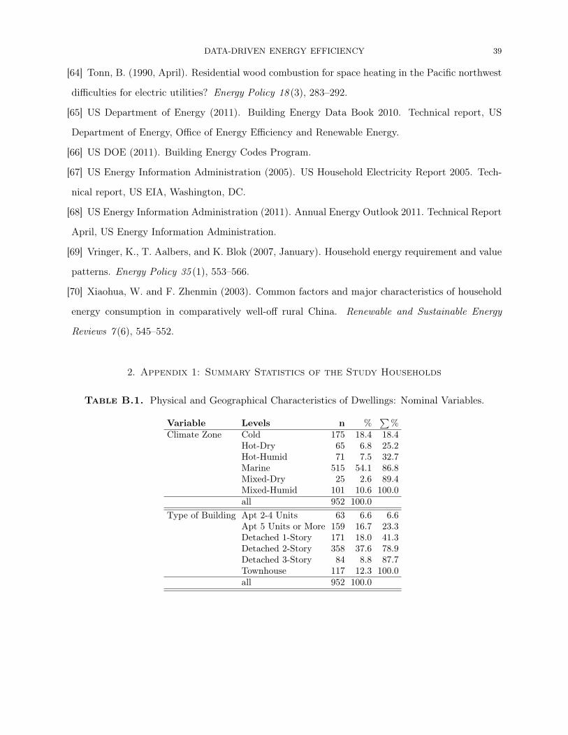
DATA-DRIVEN ENERGY EFFICIENCY 39
[64] Tonn, B. (1990, April). Residential wood combustion for space heating in the Pacific northwest
difficulties for electric utilities? Energy Policy 18 (3), 283–292.
[65] US Department of Energy (2011). Building Energy Data Book 2010. Technical report, US
Department of Energy, Office of Energy Efficiency and Renewable Energy.
[66] US DOE (2011). Building Energy Codes Program.
[67] US Energy Information Administration (2005). US Household Electricity Report 2005. Tech-
nical report, US EIA, Washington, DC.
[68] US Energy Information Administration (2011). Annual Energy Outlook 2011. Technical Report
April, US Energy Information Administration.
[69] Vringer, K., T. Aalbers, and K. Blok (2007, January). Household energy requirement and value
patterns. Energy Policy 35 (1), 553–566.
[70] Xiaohua, W. and F. Zhenmin (2003). Common factors and major characteristics of household
energy consumption in comparatively well-off rural China. Renewable and Sustainable Energy
Reviews 7 (6), 545–552.
2. Appendix 1: Summary Statistics of the Study Households
Table B.1. Physical and Geographical Characteristics of Dwellings: Nominal Variables.
Variable Levels n %∑
%Climate Zone Cold 175 18.4 18.4
Hot-Dry 65 6.8 25.2Hot-Humid 71 7.5 32.7Marine 515 54.1 86.8Mixed-Dry 25 2.6 89.4Mixed-Humid 101 10.6 100.0all 952 100.0
Type of Building Apt 2-4 Units 63 6.6 6.6Apt 5 Units or More 159 16.7 23.3Detached 1-Story 171 18.0 41.3Detached 2-Story 358 37.6 78.9Detached 3-Story 84 8.8 87.7Townhouse 117 12.3 100.0all 952 100.0
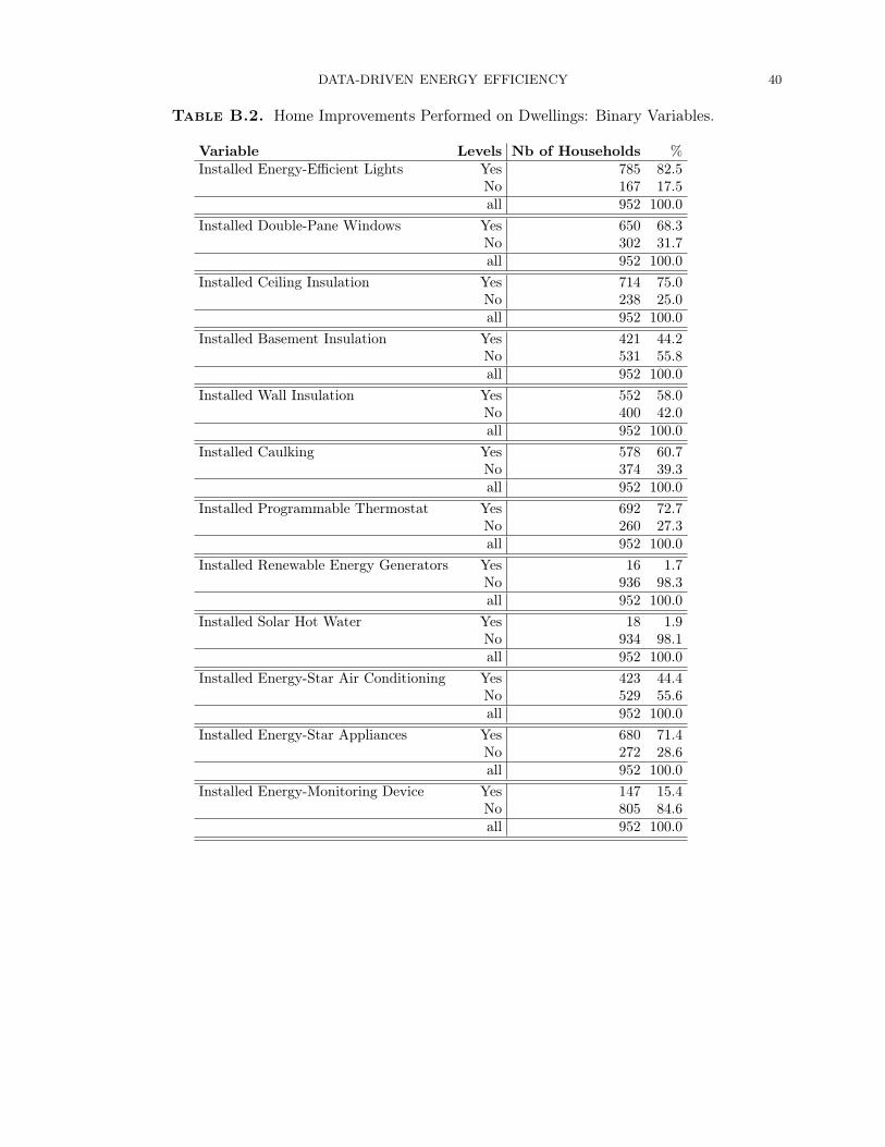
DATA-DRIVEN ENERGY EFFICIENCY 40
Table B.2. Home Improvements Performed on Dwellings: Binary Variables.
Variable Levels Nb of Households %Installed Energy-Efficient Lights Yes 785 82.5
No 167 17.5all 952 100.0
Installed Double-Pane Windows Yes 650 68.3No 302 31.7all 952 100.0
Installed Ceiling Insulation Yes 714 75.0No 238 25.0all 952 100.0
Installed Basement Insulation Yes 421 44.2No 531 55.8all 952 100.0
Installed Wall Insulation Yes 552 58.0No 400 42.0all 952 100.0
Installed Caulking Yes 578 60.7No 374 39.3all 952 100.0
Installed Programmable Thermostat Yes 692 72.7No 260 27.3all 952 100.0
Installed Renewable Energy Generators Yes 16 1.7No 936 98.3all 952 100.0
Installed Solar Hot Water Yes 18 1.9No 934 98.1all 952 100.0
Installed Energy-Star Air Conditioning Yes 423 44.4No 529 55.6all 952 100.0
Installed Energy-Star Appliances Yes 680 71.4No 272 28.6all 952 100.0
Installed Energy-Monitoring Device Yes 147 15.4No 805 84.6all 952 100.0

DATA-DRIVEN ENERGY EFFICIENCY 41
Table B.3. Fuel Use: Distribution of households possessing certain number ofmajor electric end uses.
Variable Count of End Uses Nb of Households %∑
%Electric Central Heater 0 2 0.2 0.2
1 50 5.2 5.52 186 19.5 25.03 714 75.0 100.0
all 952 100.0Electric Hot Tub 0 53 5.6 5.6
1 874 91.8 97.42 21 2.2 99.63 4 0.4 100.0
all 952 100.0Electric Water Heater 0 3 0.3 0.3
1 696 73.1 73.42 208 21.9 95.33 45 4.7 100.0
all 952 100.0Electric Clothes Dryer 0 821 86.2 86.2
1 126 13.2 99.52 5 0.5 100.0
all 952 100.0Electric Oven 0 91 9.6 9.6
1 847 89.0 98.52 13 1.4 99.93 1 0.1 100.0
all 952 100.0Electric Stove 0 94 9.9 9.9
1 845 88.8 98.62 12 1.3 99.93 1 0.1 100.0
all 952 100.0
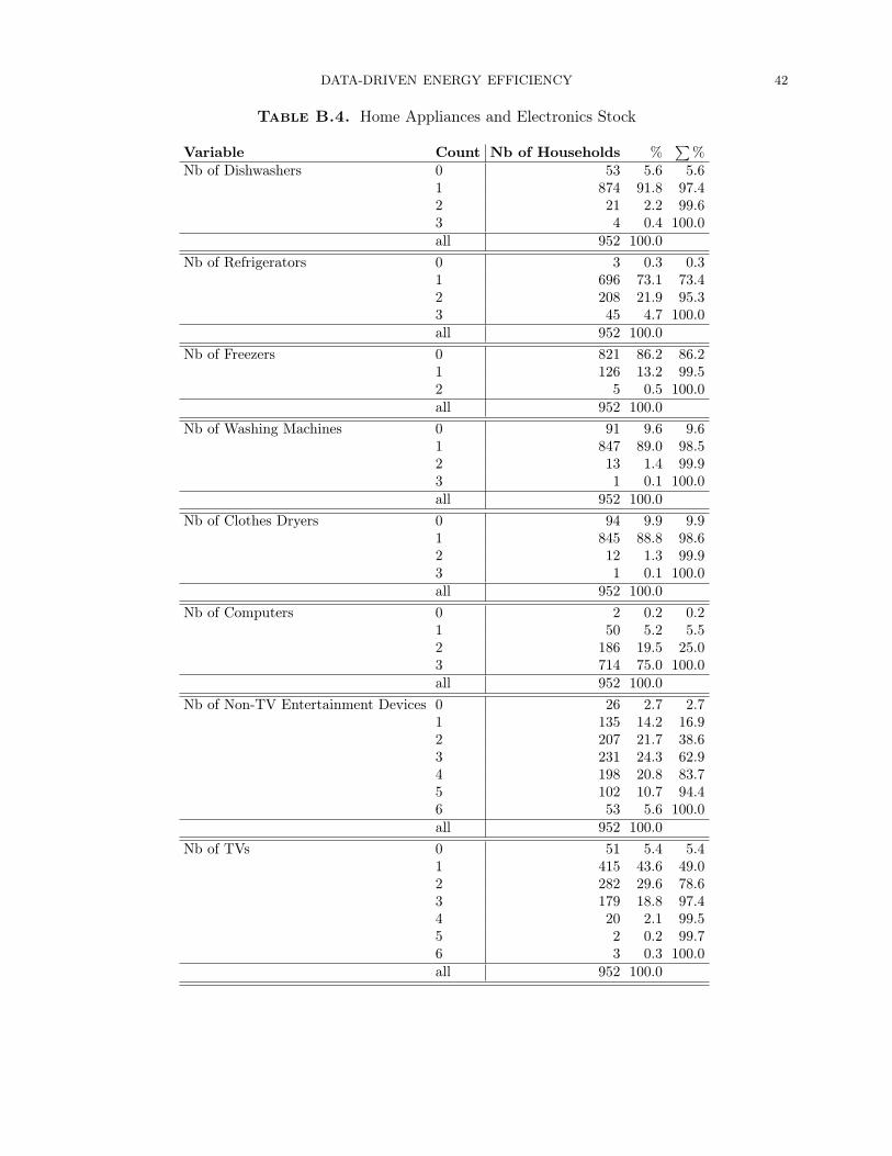
DATA-DRIVEN ENERGY EFFICIENCY 42
Table B.4. Home Appliances and Electronics Stock
Variable Count Nb of Households %∑
%Nb of Dishwashers 0 53 5.6 5.6
1 874 91.8 97.42 21 2.2 99.63 4 0.4 100.0all 952 100.0
Nb of Refrigerators 0 3 0.3 0.31 696 73.1 73.42 208 21.9 95.33 45 4.7 100.0all 952 100.0
Nb of Freezers 0 821 86.2 86.21 126 13.2 99.52 5 0.5 100.0all 952 100.0
Nb of Washing Machines 0 91 9.6 9.61 847 89.0 98.52 13 1.4 99.93 1 0.1 100.0all 952 100.0
Nb of Clothes Dryers 0 94 9.9 9.91 845 88.8 98.62 12 1.3 99.93 1 0.1 100.0all 952 100.0
Nb of Computers 0 2 0.2 0.21 50 5.2 5.52 186 19.5 25.03 714 75.0 100.0all 952 100.0
Nb of Non-TV Entertainment Devices 0 26 2.7 2.71 135 14.2 16.92 207 21.7 38.63 231 24.3 62.94 198 20.8 83.75 102 10.7 94.46 53 5.6 100.0all 952 100.0
Nb of TVs 0 51 5.4 5.41 415 43.6 49.02 282 29.6 78.63 179 18.8 97.44 20 2.1 99.55 2 0.2 99.76 3 0.3 100.0all 952 100.0

DATA-DRIVEN ENERGY EFFICIENCY 43
Table B.5. Home Major Space Conditioning End Uses
Variable Count Nb of Households %∑
%Nb of Air Conditioners 0 339 35.6 35.6
1 462 48.5 84.12 107 11.2 95.43 44 4.6 100.0all 952 100.0
Nb of Heaters 0 776 81.5 81.51 125 13.1 94.62 28 2.9 97.63 23 2.4 100.0all 952 100.0
Nb of Spas / Pools 0 829 87.1 87.11 115 12.1 99.22 7 0.7 99.93 1 0.1 100.0all 952 100.0
Nb of Acquariums and Terrariums 0 884 92.9 92.91 58 6.1 99.02 8 0.8 99.83 2 0.2 100.0all 952 100.0
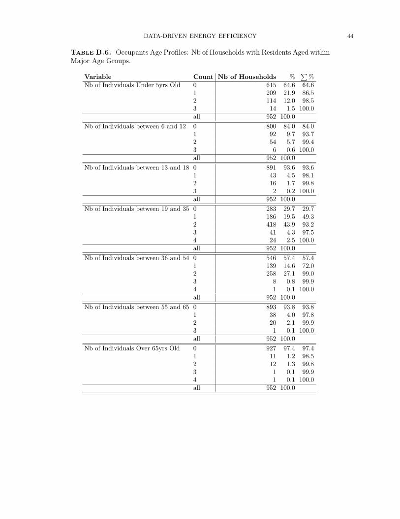
DATA-DRIVEN ENERGY EFFICIENCY 44
Table B.6. Occupants Age Profiles: Nb of Households with Residents Aged withinMajor Age Groups.
Variable Count Nb of Households %∑
%Nb of Individuals Under 5yrs Old 0 615 64.6 64.6
1 209 21.9 86.52 114 12.0 98.53 14 1.5 100.0all 952 100.0
Nb of Individuals between 6 and 12 0 800 84.0 84.01 92 9.7 93.72 54 5.7 99.43 6 0.6 100.0all 952 100.0
Nb of Individuals between 13 and 18 0 891 93.6 93.61 43 4.5 98.12 16 1.7 99.83 2 0.2 100.0all 952 100.0
Nb of Individuals between 19 and 35 0 283 29.7 29.71 186 19.5 49.32 418 43.9 93.23 41 4.3 97.54 24 2.5 100.0all 952 100.0
Nb of Individuals between 36 and 54 0 546 57.4 57.41 139 14.6 72.02 258 27.1 99.03 8 0.8 99.94 1 0.1 100.0all 952 100.0
Nb of Individuals between 55 and 65 0 893 93.8 93.81 38 4.0 97.82 20 2.1 99.93 1 0.1 100.0all 952 100.0
Nb of Individuals Over 65yrs Old 0 927 97.4 97.41 11 1.2 98.52 12 1.3 99.83 1 0.1 99.94 1 0.1 100.0all 952 100.0
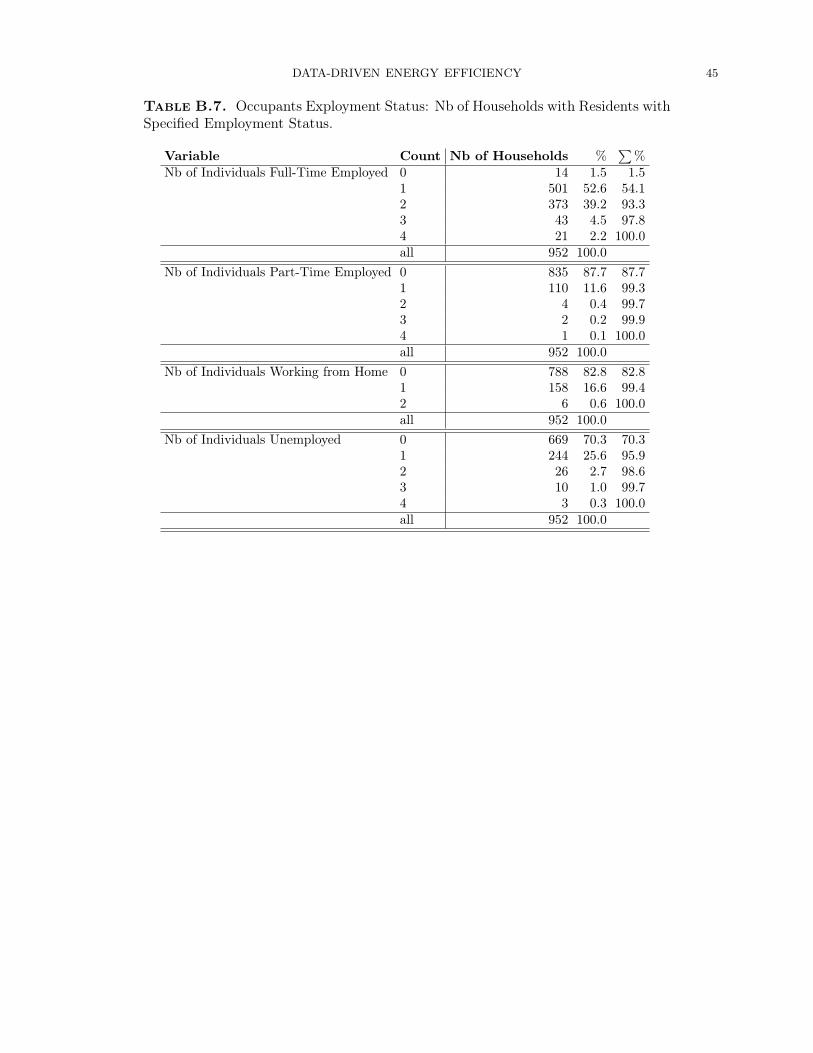
DATA-DRIVEN ENERGY EFFICIENCY 45
Table B.7. Occupants Exployment Status: Nb of Households with Residents withSpecified Employment Status.
Variable Count Nb of Households %∑
%Nb of Individuals Full-Time Employed 0 14 1.5 1.5
1 501 52.6 54.12 373 39.2 93.33 43 4.5 97.84 21 2.2 100.0all 952 100.0
Nb of Individuals Part-Time Employed 0 835 87.7 87.71 110 11.6 99.32 4 0.4 99.73 2 0.2 99.94 1 0.1 100.0all 952 100.0
Nb of Individuals Working from Home 0 788 82.8 82.81 158 16.6 99.42 6 0.6 100.0all 952 100.0
Nb of Individuals Unemployed 0 669 70.3 70.31 244 25.6 95.92 26 2.7 98.63 10 1.0 99.74 3 0.3 100.0all 952 100.0

DATA-DRIVEN ENERGY EFFICIENCY 46
Appendix: Additional Tables and Figures
More details of the model results and performance are offered in this section, along with tables
describing model parameters.
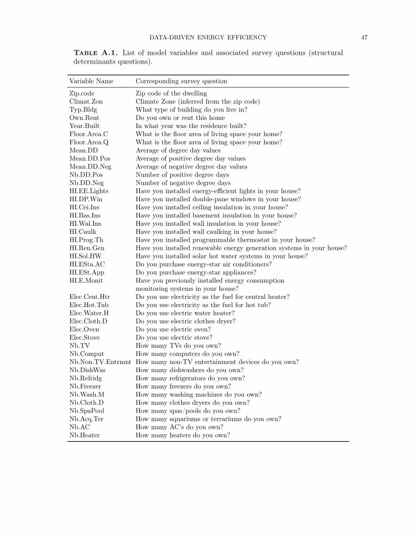
DATA-DRIVEN ENERGY EFFICIENCY 47
Table A.1. List of model variables and associated survey questions (structuraldeterminants questions).
Variable Name Corresponding survey question
Zip.code Zip code of the dwellingClimat.Zon Climate Zone (inferred from the zip code)Typ.Bldg What type of building do you live in?Own.Rent Do you own or rent this homeYear.Built In what year was the residence built?Floor.Area.C What is the floor area of living space your home?Floor.Area.Q What is the floor area of living space your home?Mean.DD Average of degree day valuesMean.DD.Pos Average of positive degree day valuesMean.DD.Neg Average of negative degree day valuesNb.DD.Pos Number of positive degree daysNb.DD.Neg Number of negative degree daysHI.EE.Lights Have you installed energy-efficient lights in your house?HI.DP.Win Have you installed double-pane windows in your house?HI.Cei.Ins Have you installed ceiling insulation in your house?HI.Bas.Ins Have you installed basement insulation in your house?HI.Wal.Ins Have you installed wall insulation in your house?HI.Caulk Have you installed wall caulking in your house?HI.Prog.Th Have you installed programmable thermostat in your house?HI.Ren.Gen Have you installed renewable energy generation systems in your house?HI.Sol.HW Have you installed solar hot water systems in your house?HI.ESta.AC Do you purchase energy-star air conditioners?HI.ESt.App Do you purchase energy-star appliances?HI.E.Monit Have you previously installed energy consumption
monitoring systems in your house?Elec.Cent.Htr Do you use electricity as the fuel for central heater?Elec.Hot.Tub Do you use electricity as the fuel for hot tub?Elec.Water.H Do you use electric water heater?Elec.Cloth.D Do you use electric clothes dryer?Elec.Oven Do you use electric oven?Elec.Stove Do you use electric stove?Nb.TV How many TVs do you own?Nb.Comput How many computers do you own?Nb.Non.TV.Entrmnt How many non-TV entertainment devices do you own?Nb.DishWas How many dishwashers do you own?Nb.Refridg How many refrigerators do you own?Nb.Freezer How many freezers do you own?Nb.Wash.M How many washing machines do you own?Nb.Cloth.D How many clothes dryers do you own?Nb.SpaPool How many spas/pools do you own?Nb.Acq.Ter How many aquariums or terrariums do you own?Nb.AC How many AC’s do you own?Nb.Heater How many heaters do you own?

DATA-DRIVEN ENERGY EFFICIENCY 48
Table A.2. List of model variables and associated survey questions (occupancylevel questions).
Variable Name Corresponding survey question
Ind.Und.5 How many individuals under 5 years old do live in the house?Ind.6.12 How many individuals between 6 and 12 years old do live in the house?Ind.13.18 How many individuals between 13 and 18 years old do live in the house?Ind.19.35 How many individuals between 19 and 35 years old do live in the house?Ind.36.54 How many individuals betweem 36 and 54 years old do live in the house?Ind.55.65 How many individuals between 55 and 65 years old do live in the house?Ind.Ove.65 How many individuals over 65 years old do live in the house?Tot.Nb.Occpnts Total number of occupantsPets.YN Do you have pets?Tot.Income What is your total annual household income?Birth.Yr What is your birth year?Gender What is your gender?
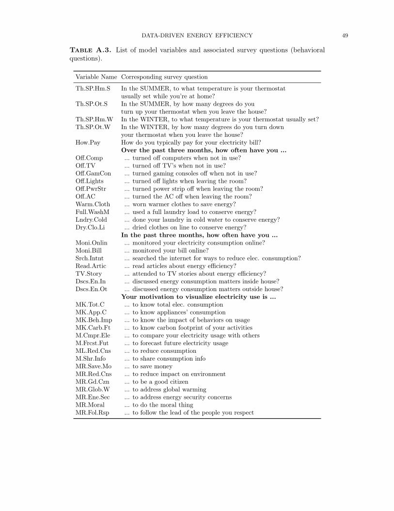
DATA-DRIVEN ENERGY EFFICIENCY 49
Table A.3. List of model variables and associated survey questions (behavioralquestions).
Variable Name Corresponding survey question
Th.SP.Hm.S In the SUMMER, to what temperature is your thermostatusually set while you’re at home?
Th.SP.Ot.S In the SUMMER, by how many degrees do youturn up your thermostat when you leave the house?
Th.SP.Hm.W In the WINTER, to what temperature is your thermostat usually set?Th.SP.Ot.W In the WINTER, by how many degrees do you turn down
your thermostat when you leave the house?How.Pay How do you typically pay for your electricity bill?
Over the past three months, how often have you ...Off.Comp ... turned off computers when not in use?Off.TV ... turned off TV’s when not in use?Off.GamCon ... turned gaming consoles off when not in use?Off.Lights ... turned off lights when leaving the room?Off.PwrStr ... turned power strip off when leaving the room?Off.AC ... turned the AC off when leaving the room?Warm.Cloth ... worn warmer clothes to save energy?Full.WashM ... used a full laundry load to conserve energy?Lndry.Cold ... done your laundry in cold water to conserve energy?Dry.Clo.Li ... dried clothes on line to conserve energy?
In the past three months, how often have you ...Moni.Onlin ... monitored your electricity consumption online?Moni.Bill ... monitored your bill online?Srch.Intnt ... searched the internet for ways to reduce elec. consumption?Read.Artic ... read articles about energy efficiency?TV.Story ... attended to TV stories about energy efficiency?Dscs.En.In ... discussed energy consumption matters inside house?Dscs.En.Ot ... discussed energy consumption matters outside house?
Your motivation to visualize electricity use is ...MK.Tot.C ... to know total elec. consumptionMK.App.C ... to know appliances’ consumptionMK.Beh.Imp ... to know the impact of behaviors on usageMK.Carb.Ft ... to know carbon footprint of your activitiesM.Cmpr.Ele ... to compare your electricity usage with othersM.Frcst.Fut ... to forecast future electricity usageML.Red.Cns ... to reduce consumptionM.Shr.Info ... to share consumption infoMR.Save.Mo ... to save moneyMR.Red.Cns ... to reduce impact on environmentMR.Gd.Czn ... to be a good citizenMR.Glob.W ... to address global warmingMR.Ene.Sec ... to address energy security concernsMR.Moral ... to do the moral thingMR.Fol.Rsp ... to follow the lead of the people you respect

DATA-DRIVEN ENERGY EFFICIENCY 50
Table A.4. Factor Loadings of Variables Representing Home Improvements Be-haviors. Note that the table only shows major loadings for each factor, to facilitateinterpretation of the factors. However, due to Jolliffe (1982), we did not discard anyloadings and created the factors using all non-zero loadings. As a result, this set offactors explains more than 80% of the total variance of the original variables.
Factor #1 2 3 4
Installed energy-efficient lights – – – –Installed double-pane windows – – – 0.73Installed ceiling insulation 0.70 – – –Installed basement insulation 0.67 – – –Installed wall insulation 0.77 – – –Installed caulking 0.53 – – –Installed programmable thermostat – – – 0.30Installed renewable energy generation – 0.93 – –Installed solar water heater – 0.73 – –Installed energy-star air conditioners – – 0.41 –Installed energy-start appliances – – 0.78 –Installed energy-monitoring devices – – – –

DATA-DRIVEN ENERGY EFFICIENCY 51
Table A.5. Factor Loadings of Variables Representing Information Seeking Be-haviors. Note that the table only shows major loadings for each factor, to facilitateinterpretation of the factors. However, due to Jolliffe (1982), we did not discard anyloadings and created the factors using all non-zero loadings. As a result, this set offactors explains more than 80% of the total variance of the original variables.
Factor #1 2 3 4 5 6 7 8 9 10 11 12
How you pay your bill – – – – – – – – – – 0.47 –Your motivation to installthe smart meter is to know...consumption consumption – 0.61 – – – – – – – – – –appliance consumption – 0.64 – – – – – – – – – -=impact of behavior changes – 0.47 – – – – – – – – – –carbon footprint of my usage – – – 0.44 – – – – – – – –compare my usage with others – – – – 0.63 – – – – – – –better forecast my future bills – – – – – 0.52 – – – – – –learn how to reduce usage – – – – – – – – – 0.79 – –share my usage info w/ others – – – – 0.55 – – – – – – –
Your motivation forreducing elec. usage is to:save money – – – – – 0.76 – – – – – –reduce energy consumption – – – – – – – – 0.49 – – –be a good world citizen – – – – – – – – 0.70 – – –address global warming – – – 0.87 – – – – – – – –support energy security – – 0.46 – – – – – – – – –do the moral thing – – 0.65 – – – – – – – – –follow the leadof the people whom I respect – – 0.58 – – – – – – – – –
How activated or exciteddo you get when talking orthinking about energy issues? 0.39 – – – – – – – – – – –
In the past 3 monthshow often did youmonitored online elec. account – – – – – – 0.63 – – – – –monitored your elec. bill – – – – – – 0.58 – – – – –searched the Internet tofind ways to reduce usage 0.58 – – – – – – – – – – –read articlesabout energy use and impact – – – – – – – 0.90 – – – –attend to TV seriesabout energy use and impact – – – – – – – – – – — 0.29discussed energy usewith adults in the house 0.61 – – – – – – – – – – –discussed energy usewith people outside the house 0.70 – – – – – – – – – – –
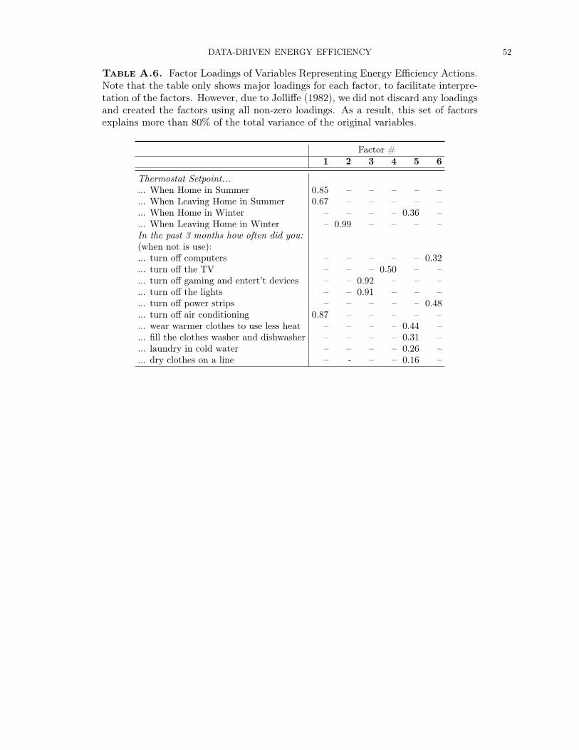
DATA-DRIVEN ENERGY EFFICIENCY 52
Table A.6. Factor Loadings of Variables Representing Energy Efficiency Actions.Note that the table only shows major loadings for each factor, to facilitate interpre-tation of the factors. However, due to Jolliffe (1982), we did not discard any loadingsand created the factors using all non-zero loadings. As a result, this set of factorsexplains more than 80% of the total variance of the original variables.
Factor #1 2 3 4 5 6
Thermostat Setpoint...... When Home in Summer 0.85 – – – – –... When Leaving Home in Summer 0.67 – – – – –... When Home in Winter – – – – 0.36 –... When Leaving Home in Winter – 0.99 – – – –In the past 3 months how often did you:(when not is use):... turn off computers – – – – – 0.32... turn off the TV – – – 0.50 – –... turn off gaming and entert’t devices – – 0.92 – – –... turn off the lights – – 0.91 – – –... turn off power strips – – – – – 0.48... turn off air conditioning 0.87 – – – – –... wear warmer clothes to use less heat – – – – 0.44 –... fill the clothes washer and dishwasher – – – – 0.31 –... laundry in cold water – – – – 0.26 –... dry clothes on a line – - – – 0.16 –

DATA-DRIVEN ENERGY EFFICIENCY 53
Table A.7. Labels assigned to each of the 22 behavioral factors. Each factor is be-lieved to represent a certain underlying behavioral characteristic that is not directlyobservable, but can be estimated using a combination of observable variables. Theselabels show our interpretation of those underlying variables based on an analysis ofthe loadings matrix, and identifying how different variables “bunched” together (allhad large factor loading values) in a factor. (EE: Energy Efficiency)
Information Seeking AttitudesFactor 1 Is a thought leaderFactor 2 Is motivated to learn about electricity
consumption and impact of behaviorFactor 3 Is motivated to reduce usage
for morality reasonsFactor 4 Is motivated to reduce usage
to address global warmingFactor 5 Is motivated to share and
compare electricity consumptionFactor 6 Is motivated to forecast
future consumption and save moneyFactor 7 Monitors bill online and in personFactor 8 Reads articles on energy efficiencyFactor 9 Is motivated to reduce
usage to be a good citizenFactor 10 Is motivated to learn
how to reduce consumptionFactor 11 Pay electricity bill after
reviewing it (payment method)Factor 12 Attends to TV stories about EE
Energy Efficiency ActionsFactor 1 Uses air conditioning efficientlyFactor 2 Uses heater efficientlyFactor 3 Turns off lights when not in useFactor 4 Turns off TV and game consoles
when not in useFactor 5 Adjusts clothing and activities to conserve electricityFactor 6 Turns off computers and
power strips when not in use
Home Improvement ActionsFactor 1 Performs home weatherization improvementsFactor 2 Installed on-site renewable energy generationFactor 3 Purchases energy star appliances and ACFactor 4 Installed double-pane windows and
programmable thermostat
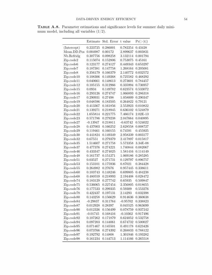
DATA-DRIVEN ENERGY EFFICIENCY 54
Table A.8. Parameter estimations and significance levels for summer daily mini-mum model, including all variables (1/2).
Estimate Std. Error t value Pr(>|t|)
(Intercept) 0.223725 0.286001 0.782254 0.43428Mean.DD.Pos 0.004987 0.00172 2.899637 0.003831Nb.Refridg 0.307756 0.098258 3.132114 0.001794Zip.code2 0.115074 0.152806 0.753075 0.45161Zip.code6 0.123177 0.274127 0.449343 0.653297Zip.code7 0.187381 0.147758 1.268164 0.205081Zip.code8 0.356179 0.166379 2.140772 0.032572Zip.code10 0.108306 0.149268 0.725582 0.468292Zip.code11 0.040661 0.148613 0.273601 0.784457Zip.code12 0.105155 0.312966 0.335994 0.736957Zip.code15 0.0934 0.149782 0.623574 0.533072Zip.code16 0.293126 0.274747 1.066893 0.286318Zip.code17 0.290931 0.27498 1.058009 0.290347Zip.code19 0.048596 0.183505 0.264822 0.79121Zip.code20 0.413367 0.161856 2.553923 0.010822Zip.code21 0.139271 0.218945 0.636102 0.524879Zip.code22 1.655814 0.221775 7.466174 2.02E-13Zip.code23 0.571786 0.279238 2.047664 0.040895Zip.code27 -0.13947 0.218811 -0.63742 0.524022Zip.code28 0.437003 0.166252 2.628558 0.008727Zip.code29 0.119461 0.160155 0.74591 0.455925Zip.code30 0.441824 0.149349 2.958339 0.003177Zip.code32 0.67551 0.279379 2.417897 0.015817Zip.code35 1.514607 0.271758 5.573358 3.34E-08Zip.code37 0.477376 0.274221 1.740844 0.082067Zip.code46 0.433347 0.274025 1.581416 0.114149Zip.code48 0.161737 0.151271 1.069186 0.285285Zip.code51 0.03527 0.271731 0.129797 0.896757Zip.code53 0.153101 0.175936 0.87021 0.384428Zip.code55 0.264982 0.27676 0.957445 0.338611Zip.code60 0.103743 0.148246 0.699805 0.484238Zip.code68 0.480559 0.218993 2.194408 0.028472Zip.code74 0.183129 0.277742 0.65935 0.509847Zip.code75 0.536065 0.227454 2.356805 0.018655Zip.code76 0.177533 0.299335 0.59309 0.553276Zip.code78 0.422437 0.197131 2.14293 0.032398Zip.code80 0.143258 0.156629 0.914636 0.360638Zip.code84 -0.29837 0.311764 -0.95702 0.338823Zip.code87 0.012928 0.28397 0.045525 0.963699Zip.code90 0.012326 0.156499 0.078759 0.937242Zip.code91 -0.01745 0.168416 -0.10362 0.917496Zip.code92 0.107262 0.171879 0.624052 0.532758Zip.code94 0.097203 0.144061 0.674732 0.500027Zip.code95 0.071467 0.145501 0.491178 0.623426Zip.code96 0.073766 0.274392 0.268833 0.788122Zip.code97 0.192792 0.14808 1.301946 0.193282Zip.code98 0.161234 0.144713 1.114166 0.265518

DATA-DRIVEN ENERGY EFFICIENCY 55
Table A.9. Parameter estimations and significance levels for summer daily mini-mum model, including all variables (2/2).
Estimate Std. Error t value Pr(>|t|)
Pets.YN 0.036294 0.008088 4.487366 8.19E-06Beh.HI.Est.App.AC 0.008055 0.004591 1.754277 0.079738Beh.EA.Htr -0.02236 0.004883 -4.5783 5.38E-06Nb.TV 0.023161 0.010063 2.301749 0.021587Floor.Area.C375 -0.2817 0.185651 -1.51739 0.129535Floor.Area.C625 -0.19031 0.175765 -1.08274 0.279228Floor.Area.C875 -0.20556 0.178062 -1.1544 0.248656Floor.Area.C1250 -0.09441 0.188198 -0.50166 0.616035Floor.Area.C1750 -0.06735 0.210592 -0.3198 0.749196Floor.Area.C2250 0.014152 0.241148 0.058686 0.953216Floor.Area.C2750 0.078228 0.272703 0.28686 0.774288Floor.Area.C3500 0.127316 0.332087 0.383381 0.701531Floor.Area.C4500 0.306527 0.410011 0.747606 0.454902Floor.Area.C5000 0.750373 0.456811 1.642634 0.100823Beh.EA.Off.Cmp.Pwr -0.05495 0.015441 -3.55881 0.000393Beh.IS.M.Rd.GlWrm -0.01099 0.003092 -3.55505 0.000398Beh.EA.Lights.Off 0.074458 0.030979 2.403524 0.016448Nb.AC.3 0.005694 0.001601 3.555552 0.000398Nb.Freezer 0.056531 0.025288 2.235474 0.025641Nb.Non.TV.Entrmnt 0.014653 0.006308 2.322939 0.020414Beh.EA.TV.Cnsl.Off -0.05851 0.028224 -2.07323 0.038447Ind.13.18 0.044237 0.012213 3.622044 0.000309Ind.Und.5 0.038401 0.009262 4.14591 3.72E-05Nb.SpaPool 0.090375 0.030114 3.001056 0.002768HI.DP.Win -0.04619 0.014532 -3.1782 0.001535Beh.HI.Win.Prg.Th 0.020886 0.008929 2.339236 0.01955HI.Wal.Ins 0.026764 0.009162 2.921276 0.003577Nb.Comput 0.035378 0.0146 2.423165 0.015591Nb.Heater.2 -0.01292 0.005313 -2.43176 0.015228Beh.IS.M.Shr.Cmpr 0.010297 0.003969 2.594579 0.009631HI.Cei.Ins -0.02105 0.010806 -1.9484 0.05169Tot.Nb.Occpnts -0.02402 0.0074 -3.24538 0.001218sqrt.Nb.Refridg -0.48487 0.245049 -1.97867 0.04817Ind.36.54 0.007259 0.004639 1.564854 0.117984Elec.Hot.Tub -0.05703 0.038076 -1.49771 0.134574HI.EE.Lights 0.019121 0.01029 1.858139 0.06349Beh.IS.Mntr.Bill -0.00807 0.005472 -1.47514 0.140539sqrt.Tot.Nb.Occpnts 0.101864 0.04977 2.046689 0.040991Child.YN -0.03168 0.01424 -2.22475 0.026356Ind.6.12 0.015844 0.008323 1.903628 0.057291HI.ESt.App 0.016674 0.01041 1.601731 0.109581HI.ESta.AC -0.01266 0.008513 -1.48665 0.137473
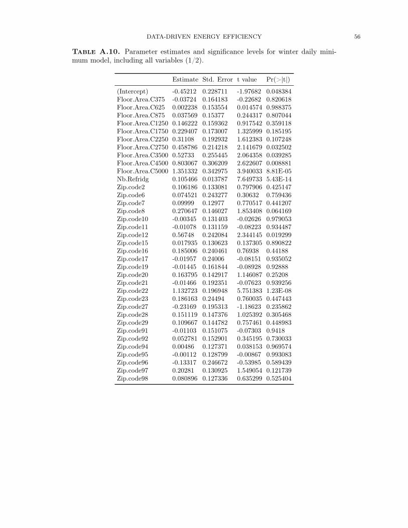
DATA-DRIVEN ENERGY EFFICIENCY 56
Table A.10. Parameter estimates and significance levels for winter daily mini-mum model, including all variables (1/2).
Estimate Std. Error t value Pr(>|t|)
(Intercept) -0.45212 0.228711 -1.97682 0.048384Floor.Area.C375 -0.03724 0.164183 -0.22682 0.820618Floor.Area.C625 0.002238 0.153554 0.014574 0.988375Floor.Area.C875 0.037569 0.15377 0.244317 0.807044Floor.Area.C1250 0.146222 0.159362 0.917542 0.359118Floor.Area.C1750 0.229407 0.173007 1.325999 0.185195Floor.Area.C2250 0.31108 0.192932 1.612383 0.107248Floor.Area.C2750 0.458786 0.214218 2.141679 0.032502Floor.Area.C3500 0.52733 0.255445 2.064358 0.039285Floor.Area.C4500 0.803067 0.306209 2.622607 0.008881Floor.Area.C5000 1.351332 0.342975 3.940033 8.81E-05Nb.Refridg 0.105466 0.013787 7.649733 5.43E-14Zip.code2 0.106186 0.133081 0.797906 0.425147Zip.code6 0.074521 0.243277 0.30632 0.759436Zip.code7 0.09999 0.12977 0.770517 0.441207Zip.code8 0.270647 0.146027 1.853408 0.064169Zip.code10 -0.00345 0.131403 -0.02626 0.979053Zip.code11 -0.01078 0.131159 -0.08223 0.934487Zip.code12 0.56748 0.242084 2.344145 0.019299Zip.code15 0.017935 0.130623 0.137305 0.890822Zip.code16 0.185006 0.240461 0.76938 0.44188Zip.code17 -0.01957 0.24006 -0.08151 0.935052Zip.code19 -0.01445 0.161844 -0.08928 0.92888Zip.code20 0.163795 0.142917 1.146087 0.25208Zip.code21 -0.01466 0.192351 -0.07623 0.939256Zip.code22 1.132723 0.196948 5.751383 1.23E-08Zip.code23 0.186163 0.24494 0.760035 0.447443Zip.code27 -0.23169 0.195313 -1.18623 0.235862Zip.code28 0.151119 0.147376 1.025392 0.305468Zip.code29 0.109667 0.144782 0.757461 0.448983Zip.code91 -0.01103 0.151075 -0.07303 0.9418Zip.code92 0.052781 0.152901 0.345195 0.730033Zip.code94 0.00486 0.127371 0.038153 0.969574Zip.code95 -0.00112 0.128799 -0.00867 0.993083Zip.code96 -0.13317 0.246672 -0.53985 0.589439Zip.code97 0.20281 0.130925 1.549054 0.121739Zip.code98 0.080896 0.127336 0.635299 0.525404

DATA-DRIVEN ENERGY EFFICIENCY 57
Table A.11. Parameter estimates and significance levels for winter daily mini-mum model, including all variables (2/2).
Estimate Std. Error t value Pr(>|t|)
Beh.HI.Est.App.AC 0.013306 0.00328 4.056475 5.44E-05Beh.EA.Htr -0.01458 0.00428 -3.40539 0.000692Nb.Non.TV.Entrmnt 0.012522 0.005568 2.248928 0.024771Nb.SpaPool 0.101823 0.019797 5.143489 3.35E-07Beh.IS.M.Rd.GlWrm -0.00987 0.002504 -3.94218 8.74E-05sqrt.Nb.DD.Neg 0.036687 0.007049 5.204531 2.44E-07Pets.YN 0.021269 0.00716 2.9703 0.003058Beh.EA.Off.Cmp.Pwr -0.04786 0.013625 -3.51266 0.000467Ind.13.18 0.022115 0.008757 2.525387 0.011737Mean.DD.Pos 0.006048 0.002368 2.554218 0.010815Nb.Comput 0.029687 0.012807 2.318101 0.020679Mean.DD.Neg -0.0019 0.001919 -0.99114 0.321896Nb.TV 0.024514 0.008898 2.754941 0.005995Birth.Yr1960 - 1969 0.019427 0.042935 0.452489 0.651032Birth.Yr1970 - 1979 -0.02463 0.042316 -0.58201 0.560715Birth.Yr1980 and after -0.05148 0.043831 -1.17446 0.240536Birth.YrBefore 1950 0.254568 0.113062 2.251578 0.024602Birth.YrPrefer not to answer -0.00166 0.054893 -0.03015 0.975952HI.DP.Win -0.01545 0.008805 -1.75496 0.079625Nb.Freezer 0.049781 0.021803 2.2832 0.022663Elec.Oven 0.053364 0.01825 2.924149 0.003545Nb.AC.2 0.007813 0.004225 1.849094 0.06479Beh.EA.TV.Cnsl.Off -0.0379 0.024655 -1.53702 0.124659HI.Cei.Ins -0.02788 0.009642 -2.89191 0.003926HI.Wal.Ins 0.024647 0.00809 3.046573 0.002386Ind.Und.5 0.002873 0.005241 0.548172 0.583717sqrt.Nb.DD.Pos.2 0.01776 0.006108 2.907685 0.003735sqrt.Mean.DD.Pos -0.06446 0.030019 -2.14732 0.032049Ind.55.65 -0.01651 0.009118 -1.81095 0.0705Tot.Income$150,000 - $250,000 0.012106 0.020796 0.582133 0.560631Tot.Income$250,000 or more -0.03257 0.024578 -1.32506 0.185504Tot.Income$30,000 - $50,000 -0.1421 0.106788 -1.33072 0.183637Tot.Income$50,000 - $75,000 -0.13094 0.057514 -2.27668 0.023052Tot.Income$75,000 - $100,000 -0.00649 0.033177 -0.19547 0.845072Tot.IncomeDon’t know / Prefer not to answer -0.0246 0.023545 -1.0449 0.296365Beh.EA.En.Csrv -0.0167 0.010385 -1.60766 0.10828Elec.Stove -0.03394 0.019953 -1.70099 0.089309Mean.DD.Pos.2 0.0006 0.000379 1.584375 0.113479Nb.P.T.Emp -0.01546 0.009164 -1.68746 0.091879sqrt.Tot.Nb.Occpnts 0.056205 0.027191 2.067049 0.03903Ind.Ove.65 -0.01562 0.009743 -1.60301 0.109303HI.Bas.Ins -0.01087 0.007602 -1.4305 0.152938
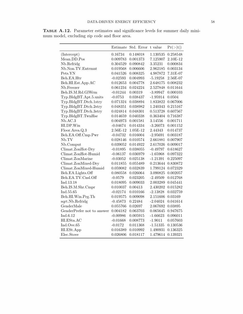
DATA-DRIVEN ENERGY EFFICIENCY 58
Table A.12. Parameter estimates and significance levels for summer daily mini-mum model, excluding zip code and floor area.
Estimate Std. Error t value Pr(>|t|)
(Intercept) 0.16734 0.148018 1.130535 0.258548Mean.DD.Pos 0.009783 0.001373 7.125907 2.10E-12Nb.Refridg 0.304529 0.090842 3.35231 0.000834Nb.Non.TV.Entrmnt 0.019568 0.006606 2.962185 0.003134Pets.YN 0.041526 0.008325 4.987872 7.31E-07Beh.EA.Htr -0.02593 0.004993 -5.19258 2.56E-07Beh.HI.Est.App.AC 0.012653 0.004778 2.648175 0.008232Nb.Freezer 0.061234 0.024224 2.527848 0.011644Beh.IS.M.Rd.GlWrm -0.01244 0.00319 -3.89947 0.000103Typ.BldgBT.Apt.5.units -0.0753 0.038437 -1.95914 0.0504Typ.BldgBT.Dtch.1stry 0.071324 0.038894 1.833822 0.067006Typ.BldgBT.Dtch.2stry 0.048351 0.038982 1.240343 0.215167Typ.BldgBT.Dtch.3stry 0.024814 0.048301 0.513728 0.607567Typ.BldgBT.TwnHse 0.014659 0.040338 0.363404 0.716387Nb.AC.3 0.004973 0.001581 3.14556 0.001711HI.DP.Win -0.04674 0.014334 -3.26073 0.001152Floor.Area.Q.3 2.56E-12 1.05E-12 2.44343 0.014737Beh.EA.Off.Cmp.Pwr -0.04732 0.016004 -2.95691 0.003187Nb.TV 0.028146 0.010574 2.661881 0.007907Nb.Comput 0.039052 0.014922 2.617026 0.009017Climat.ZonHot-Dry -0.01895 0.038055 -0.49797 0.618627Climat.ZonHot-Humid -0.06137 0.036979 -1.65968 0.097322Climat.ZonMarine -0.03052 0.025138 -1.21391 0.225097Climat.ZonMixed-Dry 0.011855 0.055489 0.213644 0.830872Climat.ZonMixed-Humid 0.059082 0.032839 1.799124 0.072329Beh.EA.Lights.Off 0.080558 0.026064 3.090825 0.002057Beh.EA.TV.Cnsl.Off -0.0579 0.023205 -2.49509 0.012768Ind.13.18 0.018095 0.009033 2.003289 0.045441Beh.IS.M.Shr.Cmpr 0.010037 0.00413 2.430202 0.015282Ind.55.65 -0.02174 0.010166 -2.13828 0.032759Beh.HI.Win.Prg.Th 0.019575 0.009098 2.151606 0.03169sqrt.Nb.Refridg -0.45873 0.22484 -2.04024 0.041614GenderMale 0.055766 0.02697 2.067692 0.03895GenderPrefer not to answer 0.004182 0.063703 0.065645 0.947675Ind.6.12 -0.00986 0.005915 -1.66623 0.096011HI.ESta.AC -0.01668 0.008773 -1.9011 0.057603Ind.Ove.65 -0.0172 0.011368 -1.51335 0.130536HI.ESt.App 0.016389 0.010992 1.490931 0.136325Elec.Stove 0.026806 0.018117 1.479614 0.139321

DATA-DRIVEN ENERGY EFFICIENCY 59
Table A.13. Parameter estimates and significance levels for winter daily mini-mum model, excluding zip code and floor area.
Estimate Std. Error t value Pr(>|t|)
(Intercept) 0.24903 0.136532 1.823971 0.068481Beh.EA.Lights.Off 0.045672 0.023264 1.963183 0.049926Nb.Refridg 0.239485 0.078513 3.05026 0.002352Nb.Non.TV.Entrmnt 0.019209 0.005645 3.402914 0.000696Beh.HI.Est.App.AC 0.015447 0.003374 4.577654 5.35E-06Beh.EA.Htr -0.01713 0.00435 -3.93805 8.84E-05Pets.YN 0.028545 0.007161 3.985873 7.26E-05Beh.IS.M.Rd.GlWrm -0.01046 0.002628 -3.97832 7.49E-05Mean.DD.Pos 0.01692 0.002594 6.521936 1.14E-10Mean.DD -0.00682 0.001271 -5.36844 1.01E-07Nb.SpaPool 0.075608 0.020432 3.70055 0.000228Nb.Freezer 0.054141 0.020619 2.62584 0.008787Nb.Comput 0.043829 0.01285 3.410666 0.000676Beh.EA.En.Csrv -0.02335 0.010131 -2.3047 0.021405Nb.TV 0.019884 0.00898 2.214215 0.027059sqrt.Mean.DD.Pos -0.05377 0.020637 -2.60547 0.009323Beh.EA.Off.Cmp.Pwr -0.033 0.013824 -2.38723 0.017177Ind.13.18 0.018431 0.007763 2.37425 0.017789HI.DP.Win -0.01738 0.008314 -2.0903 0.036865Typ.BldgBT.Apt.5.units -0.07556 0.0332 -2.27593 0.02308Typ.BldgBT.Dtch.1stry 0.052881 0.033579 1.574828 0.11564Typ.BldgBT.Dtch.2stry 0.047881 0.033583 1.425768 0.154275Typ.BldgBT.Dtch.3stry 0.051321 0.041351 1.241084 0.214891Typ.BldgBT.TwnHse 0.008521 0.034978 0.243602 0.807593Floor.Area.Q.3 2.99E-12 9.02E-13 3.317104 0.000945Nb.Heater 0.011977 0.006855 1.747269 0.080925Beh.EA.TV.Cnsl.Off -0.04683 0.020954 -2.23488 0.025665GenderMale 0.052582 0.023244 2.262174 0.023919GenderPrefer not to answer 0.017293 0.054611 0.316661 0.751573sqrt.Nb.Refridg -0.34216 0.194028 -1.76348 0.078152Nb.AC.2 0.00707 0.003976 1.778162 0.075708Elec.Oven 0.023104 0.014899 1.550679 0.121323Beh.IS.Pay.Meth 0.024823 0.016147 1.537301 0.124564
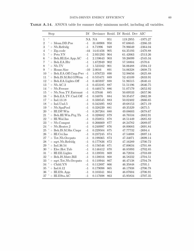
DATA-DRIVEN ENERGY EFFICIENCY 60
Table A.14. ANOVA table for summer daily minimum model, including all variables.
Step Df Deviance Resid. Df Resid. Dev AIC
1 ’ NA NA 951 119.2955 -1975.272 ’ + Mean.DD.Pos -1 31.60908 950 87.68645 -2266.333 ’ + Nb.Refridg -1 8.71996 949 78.96649 -2364.044 ’ + Zip.code -44 14.61456 905 64.35193 -2470.885 ’ + Pets.YN -1 2.931293 904 61.42063 -2513.266 ’ + Beh.HI.Est.App.AC -1 2.159643 903 59.26099 -2545.347 ’ + Beh.EA.Htr -1 1.672949 902 57.58804 -2570.68 ’ + Nb.TV -1 1.523162 901 56.06488 -2594.129 ’ + House.Size -10 2.0016 891 54.06328 -2608.7310 ’ + Beh.EA.Off.Cmp.Pwr -1 1.076723 890 52.98656 -2625.8811 ’ + Beh.IS.M.Rd.GlWrm -1 0.555471 889 52.43109 -2633.9112 ’ + Beh.EA.Lights.Off -1 0.465937 888 51.96515 -2640.4113 ’ + Nb.AC.3 -1 0.453185 887 51.51196 -2646.7514 ’ + Nb.Freezer -1 0.440174 886 51.07179 -2652.9215 ’ + Nb.Non.TV.Entrmnt -1 0.37646 885 50.69533 -2657.9616 ’ + Beh.EA.TV.Cnsl.Off -1 0.34076 884 50.35457 -2662.3817 ’ + Ind.13.18 -1 0.330545 883 50.02402 -2666.6518 ’ + Ind.Und.5 -1 0.342495 882 49.68153 -2671.1919 ’ + Nb.SpaPool -1 0.328239 881 49.35329 -2675.520 ’ + HI.DP.Win -1 0.267264 880 49.08603 -2678.6721 ’ + Beh.HI.Win.Prg.Th -1 0.320682 879 48.76534 -2682.9122 ’ + HI.Wal.Ins -1 0.250851 878 48.51449 -2685.8223 ’ + Nb.Comput -1 0.266669 877 48.24782 -2689.0724 ’ + Nb.Heater.2 -1 0.240997 876 48.00683 -2691.8425 ’ + Beh.IS.M.Shr.Cmpr -1 0.229504 875 47.77732 -2694.426 ’ + HI.Cei.Ins -1 0.237245 874 47.54008 -2697.1427 ’ + Tot.Nb.Occpnts -1 0.199365 873 47.34071 -2699.1428 ’ + sqrt.Nb.Refridg -1 0.177826 872 47.16289 -2700.7229 ’ + Ind.36.54 -1 0.156546 871 47.00634 -2701.8830 ’ + Elec.Hot.Tub -1 0.146412 870 46.85993 -2702.8531 ’ + HI.EE.Lights -1 0.139591 869 46.72034 -2703.6932 ’ + Beh.IS.Mntr.Bill -1 0.138016 868 46.58232 -2704.5133 ’ + sqrt.Tot.Nb.Occpnts -1 0.110944 867 46.47138 -2704.7834 ’ + Child.YN -1 0.112897 866 46.35848 -2705.135 ’ + Ind.6.12 -1 0.179098 865 46.17938 -2706.7836 ’ + HI.ESt.App -1 0.103341 864 46.07604 -2706.9137 ’ + HI.ESta.AC -1 0.117698 863 45.95834 -2707.35
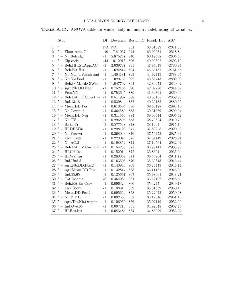
DATA-DRIVEN ENERGY EFFICIENCY 61
Table A.15. ANOVA table for winter daily minimum model, using all variables.
Step Df Deviance Resid. Df Resid. Dev AIC
1 ’ NA NA 951 83.81089 -2311.362 ’ + Floor.Area.C -10 17.81057 941 66.00031 -2518.83 ’ + Nb.Refridg -1 5.875237 940 60.12508 -2605.564 ’ + Zip.code -44 10.12915 896 49.99592 -2693.195 ’ + Beh.HI.Est.App.AC -1 2.039737 895 47.95619 -2730.846 ’ + Beh.EA.Htr -1 1.624814 894 46.33137 -2761.657 ’ + Nb.Non.TV.Entrmnt -1 1.404181 893 44.92719 -2788.958 ’ + Nb.SpaPool -1 1.029766 892 43.89743 -2809.039 ’ + Beh.IS.M.Rd.GlWrm -1 1.047702 891 42.84972 -2830.0210 ’ + sqrt.Nb.DD.Neg -1 0.752466 890 42.09726 -2844.8911 ’ + Pets.YN -1 0.753645 889 41.34361 -2860.0912 ’ + Beh.EA.Off.Cmp.Pwr -1 0.511967 888 40.83165 -2869.9513 ’ + Ind.13.18 -1 0.5398 887 40.29185 -2880.6214 ’ + Mean.DD.Pos -1 0.610564 886 39.68128 -2893.1615 ’ + Nb.Comput -1 0.364589 885 39.31669 -2899.9416 ’ + Mean.DD.Neg -1 0.311556 884 39.00514 -2905.5217 ’ + Nb.TV -1 0.296896 883 38.70824 -2910.7918 ’ + Birth.Yr -5 0.577538 878 38.1307 -2915.119 ’ + HI.DP.Win -1 0.298128 877 37.83258 -2920.5820 ’ + Nb.Freezer -1 0.268043 876 37.56453 -2925.3421 ’ + Elec.Oven -1 0.22004 875 37.34449 -2928.9422 ’ + Nb.AC.2 -1 0.198852 874 37.14564 -2932.0223 ’ + Beh.EA.TV.Cnsl.Off -1 0.154236 873 36.99141 -2933.9824 ’ + HI.Cei.Ins -1 0.15201 872 36.8394 -2935.925 ’ + HI.Wal.Ins -1 0.280359 871 36.55904 -2941.1726 ’ + Ind.Und.5 -1 0.163606 870 36.39543 -2943.4427 ’ + sqrt.Nb.DD.Pos.2 -1 0.140943 869 36.25449 -2945.1428 ’ + sqrt.Mean.DD.Pos -1 0.142814 868 36.11167 -2946.929 ’ + Ind.55.65 -1 0.125667 867 35.98601 -2948.2130 ’ + Tot.Income -6 0.464985 861 35.52102 -2948.631 ’ + Beh.EA.En.Csrv -1 0.096326 860 35.4247 -2949.1832 ’ + Elec.Stove -1 0.10831 859 35.31639 -2950.133 ’ + Mean.DD.Pos.2 -1 0.095664 858 35.22072 -2950.6834 ’ + Nb.P.T.Emp -1 0.092558 857 35.12816 -2951.1835 ’ + sqrt.Tot.Nb.Occpnts -1 0.106969 856 35.02119 -2952.0936 ’ + Ind.Ove.65 -1 0.097718 855 34.92348 -2952.7537 ’ + HI.Bas.Ins -1 0.083483 854 34.83999 -2953.02
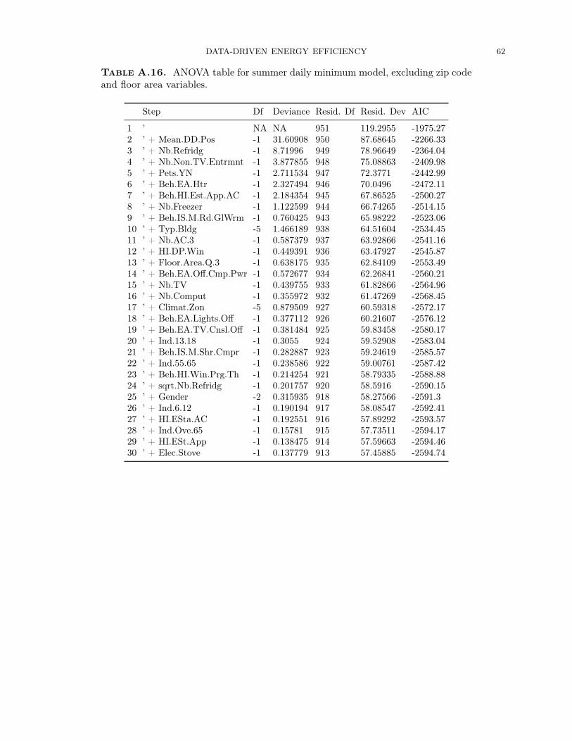
DATA-DRIVEN ENERGY EFFICIENCY 62
Table A.16. ANOVA table for summer daily minimum model, excluding zip codeand floor area variables.
Step Df Deviance Resid. Df Resid. Dev AIC
1 ’ NA NA 951 119.2955 -1975.272 ’ + Mean.DD.Pos -1 31.60908 950 87.68645 -2266.333 ’ + Nb.Refridg -1 8.71996 949 78.96649 -2364.044 ’ + Nb.Non.TV.Entrmnt -1 3.877855 948 75.08863 -2409.985 ’ + Pets.YN -1 2.711534 947 72.3771 -2442.996 ’ + Beh.EA.Htr -1 2.327494 946 70.0496 -2472.117 ’ + Beh.HI.Est.App.AC -1 2.184354 945 67.86525 -2500.278 ’ + Nb.Freezer -1 1.122599 944 66.74265 -2514.159 ’ + Beh.IS.M.Rd.GlWrm -1 0.760425 943 65.98222 -2523.0610 ’ + Typ.Bldg -5 1.466189 938 64.51604 -2534.4511 ’ + Nb.AC.3 -1 0.587379 937 63.92866 -2541.1612 ’ + HI.DP.Win -1 0.449391 936 63.47927 -2545.8713 ’ + Floor.Area.Q.3 -1 0.638175 935 62.84109 -2553.4914 ’ + Beh.EA.Off.Cmp.Pwr -1 0.572677 934 62.26841 -2560.2115 ’ + Nb.TV -1 0.439755 933 61.82866 -2564.9616 ’ + Nb.Comput -1 0.355972 932 61.47269 -2568.4517 ’ + Climat.Zon -5 0.879509 927 60.59318 -2572.1718 ’ + Beh.EA.Lights.Off -1 0.377112 926 60.21607 -2576.1219 ’ + Beh.EA.TV.Cnsl.Off -1 0.381484 925 59.83458 -2580.1720 ’ + Ind.13.18 -1 0.3055 924 59.52908 -2583.0421 ’ + Beh.IS.M.Shr.Cmpr -1 0.282887 923 59.24619 -2585.5722 ’ + Ind.55.65 -1 0.238586 922 59.00761 -2587.4223 ’ + Beh.HI.Win.Prg.Th -1 0.214254 921 58.79335 -2588.8824 ’ + sqrt.Nb.Refridg -1 0.201757 920 58.5916 -2590.1525 ’ + Gender -2 0.315935 918 58.27566 -2591.326 ’ + Ind.6.12 -1 0.190194 917 58.08547 -2592.4127 ’ + HI.ESta.AC -1 0.192551 916 57.89292 -2593.5728 ’ + Ind.Ove.65 -1 0.15781 915 57.73511 -2594.1729 ’ + HI.ESt.App -1 0.138475 914 57.59663 -2594.4630 ’ + Elec.Stove -1 0.137779 913 57.45885 -2594.74

DATA-DRIVEN ENERGY EFFICIENCY 63
Table A.17. ANOVA table for winter daily minimum model, excluding zip codeand floor area variables.
Step Df Deviance Resid. Df Resid. Dev AIC
1 ’ NA NA 951 83.81089 -2311.362 ’ + Beh.EA.Lights.Off -1 15.94699 950 67.8639 -2510.293 ’ + Nb.Refridg -1 6.015745 949 61.84815 -2596.664 ’ + Nb.Non.TV.Entrmnt -1 3.286682 948 58.56147 -2646.645 ’ + Beh.HI.Est.App.AC -1 2.38564 947 56.17583 -2684.236 ’ + Beh.EA.Htr -1 1.903443 946 54.27239 -2715.057 ’ + Pets.YN -1 1.218338 945 53.05405 -2734.678 ’ + Beh.IS.M.Rd.GlWrm -1 1.344991 944 51.70906 -2757.119 ’ + Mean.DD.Pos -1 0.95161 943 50.75745 -2772.7910 ’ + Mean.DD -1 1.27528 942 49.48217 -2795.0211 ’ + Nb.SpaPool -1 0.850469 941 48.6317 -2809.5212 ’ + Nb.Freezer -1 0.552625 940 48.07908 -2818.413 ’ + Nb.Comput -1 0.519036 939 47.56004 -2826.7414 ’ + Beh.EA.En.Csrv -1 0.438643 938 47.1214 -2833.5615 ’ + Nb.TV -1 0.377906 937 46.74349 -2839.2216 ’ + sqrt.Mean.DD.Pos -1 0.289743 936 46.45375 -2843.1417 ’ + Beh.EA.Off.Cmp.Pwr -1 0.321233 935 46.13251 -2847.7518 ’ + Ind.13.18 -1 0.259776 934 45.87274 -2851.1219 ’ + HI.DP.Win -1 0.22949 933 45.64325 -2853.920 ’ + Typ.Bldg -5 0.610084 928 45.03316 -2856.7121 ’ + Floor.Area.Q.3 -1 0.428254 927 44.60491 -2863.8122 ’ + Nb.Heater -1 0.23409 926 44.37082 -2866.8223 ’ + Beh.EA.TV.Cnsl.Off -1 0.198894 925 44.17193 -2869.0924 ’ + Gender -2 0.280924 923 43.891 -2871.1725 ’ + sqrt.Nb.Refridg -1 0.151642 922 43.73936 -2872.4626 ’ + Nb.AC.2 -1 0.13003 921 43.60933 -2873.327 ’ + Elec.Oven -1 0.119799 920 43.48953 -2873.9128 ’ + Beh.IS.Pay.Meth -1 0.111551 919 43.37798 -2874.36

DATA-DRIVEN ENERGY EFFICIENCY 64
●
●
●
●
●
●
●
●
●●
● ● ● ● ● ● ● ● ● ● ● ● ● ● ● ● ● ● ● ● ● ● ● ● ● ● ●
4050
6070
8090
100
% Residual Deviance for Forward Stepwise Regressionon Min−Summer kWh for All Users | All Variables (Baseline) | R2= 0.58
% R
esid
ual D
evia
nce
Inte
rcep
t
+ M
ean.
DD
.Pos
+ N
b.R
efrid
g+
Zip.
code
+ Pe
ts.Y
N
+ Be
h.H
I.Est
.App
.AC
+ Be
h.EA
.Htr
+ N
b.TV
+ Fl
oor.A
rea.
C
+ Be
h.EA
.Off.
Cm
p.Pw
r
+ Be
h.IS
.M.R
d.G
lWrm
+ Be
h.EA
.Lig
hts.
Off
+ N
b.AC
.3
+ N
b.Fr
eeze
r
+ N
b.N
on.T
V.En
trmnt
+ Be
h.EA
.TV.
Cns
l.Off
+ In
d.13
.18
+ In
d.U
nd.5
+ N
b.Sp
aPoo
l
+ H
I.DP.
Win
+ Be
h.H
I.Win
.Prg
.Th
+ H
I.Wal
.Ins
+ N
b.C
ompu
t
+ N
b.H
eate
r.2
+ Be
h.IS
.M.S
hr.C
mpr
+ H
I.Cei
.Ins
+ To
t.Nb.
Occ
pnts
+ sq
rt.N
b.R
efrid
g+
Ind.
36.5
4
+ El
ec.H
ot.T
ub
+ H
I.EE.
Ligh
ts
+ Be
h.IS
.Mnt
r.Bill
+ sq
rt.To
t.Nb.
Occ
pnts
+ C
hild
.YN
+ In
d.6.
12
+ H
I.ESt
.App
+ H
I.ESt
a.AC
●
●
●
●
●
●
●●
●● ● ● ● ● ● ● ● ● ● ● ● ● ● ● ● ● ● ● ● ● ● ● ● ● ● ● ●
Figure A.1. Residual deviance versus model step plot for summer daily mini-mum model. This plot shows the residual deviance of the model as new variables(determinants) are added to the daily minimum summer stepwise model. The firstfew determinants explain most of the variability. Also note that Floor Area is thesame as House Size explained in the paper.
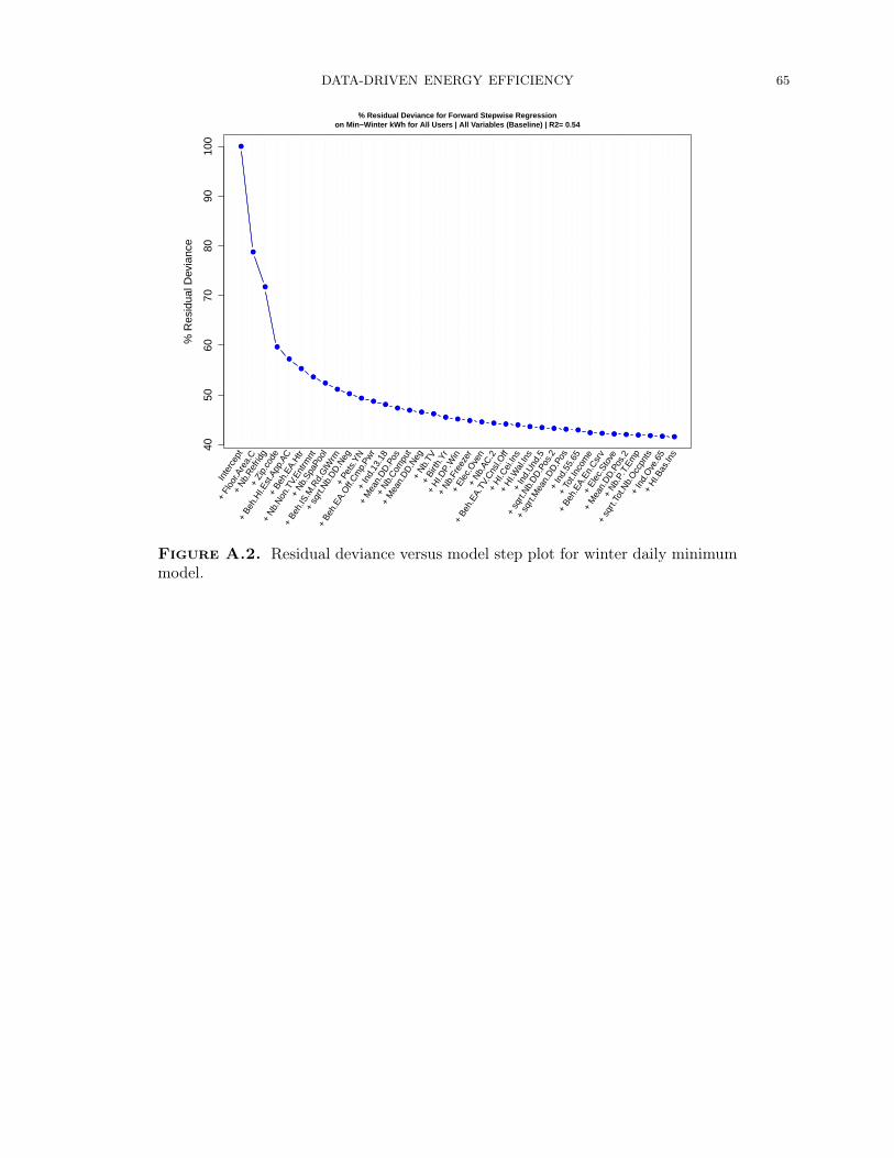
DATA-DRIVEN ENERGY EFFICIENCY 65
●
●
●
●
●
●
●
●
●●
●●
●●
● ● ●● ● ● ● ● ● ● ● ● ● ● ●
● ● ● ● ● ● ● ●
4050
6070
8090
100
% Residual Deviance for Forward Stepwise Regressionon Min−Winter kWh for All Users | All Variables (Baseline) | R2= 0.54
% R
esid
ual D
evia
nce
Inte
rcep
t
+ Fl
oor.A
rea.
C
+ N
b.R
efrid
g+
Zip.
code
+ Be
h.H
I.Est
.App
.AC
+ Be
h.EA
.Htr
+ N
b.N
on.T
V.En
trmnt
+ N
b.Sp
aPoo
l
+ Be
h.IS
.M.R
d.G
lWrm
+ sq
rt.N
b.D
D.N
eg+
Pets
.YN
+ Be
h.EA
.Off.
Cm
p.Pw
r+
Ind.
13.1
8
+ M
ean.
DD
.Pos
+ N
b.C
ompu
t
+ M
ean.
DD
.Neg
+ N
b.TV
+ Bi
rth.Y
r
+ H
I.DP.
Win
+ N
b.Fr
eeze
r
+ El
ec.O
ven
+ N
b.AC
.2
+ Be
h.EA
.TV.
Cns
l.Off
+ H
I.Cei
.Ins
+ H
I.Wal
.Ins
+ In
d.U
nd.5
+ sq
rt.N
b.D
D.P
os.2
+ sq
rt.M
ean.
DD
.Pos
+ In
d.55
.65
+ To
t.Inc
ome
+ Be
h.EA
.En.
Csr
v
+ El
ec.S
tove
+ M
ean.
DD
.Pos
.2
+ N
b.P.
T.Em
p
+ sq
rt.To
t.Nb.
Occ
pnts
+ In
d.O
ve.6
5
+ H
I.Bas
.Ins
●
●
●
●
●
●
●●
●●
●●
●● ● ● ●
● ● ● ● ● ● ● ● ● ● ● ●● ● ● ● ● ● ● ●
Figure A.2. Residual deviance versus model step plot for winter daily minimummodel.

DATA-DRIVEN ENERGY EFFICIENCY 66
Variables (Baseline).pdf
0.0
0.5
1.0
1.5
Regression Coefficients for Forward Stepwise Regressionon Min kWh for All Users | All Variables (Baseline) | R2= 0.57
Reg
ress
ion
Coe
ffici
ent
(Inte
rcep
t)
Mea
n.DD.P
os
Nb.Ref
ridg
Zip.co
de2
Zip.co
de6
Zip.co
de7
Zip.co
de8
Zip.co
de10
Zip.co
de11
Zip.co
de12
Zip.co
de15
Zip.co
de16
Zip.co
de17
Zip.co
de19
Zip.co
de20
Zip.co
de21
Zip.co
de22
Zip.co
de23
Zip.co
de27
Zip.co
de28
Zip.co
de29
Zip.co
de30
Zip.co
de32
Zip.co
de35
Zip.co
de37
Zip.co
de46
Zip.co
de48
Zip.co
de51
Zip.co
de53
Zip.co
de55
Zip.co
de60
Zip.co
de68
Zip.co
de74
Zip.co
de75
Zip.co
de76
Zip.co
de78
Zip.co
de80
Zip.co
de84
Zip.co
de87
Zip.co
de90
Zip.co
de91
Zip.co
de92
Zip.co
de94
Zip.co
de95
Zip.co
de96
Zip.co
de97
Zip.co
de98
Beh.H
I.Est.
App.A
C
Nb.Non
.TV.
Entrm
nt
Beh.E
A.Htr
Floor.A
rea.
C375
Floor.A
rea.
C625
Floor.A
rea.
C875
Floor.A
rea.
C1250
Floor.A
rea.
C1750
Floor.A
rea.
C2250
Floor.A
rea.
C2750
Floor.A
rea.
C3500
Floor.A
rea.
C4500
Floor.A
rea.
C5000
Beh.E
A.Off.C
mp.P
wr
Nb.AC.3
Nb.Spa
Pool
Beh.IS
.M.R
d.GlW
rm
Ind.
13.1
8
Nb.Fre
ezer
Nb.TV
sqrt.
Mea
n.DD.P
os
HI.DP.W
in
Beh.H
I.Win.
Prg.T
h
Ind.
Und.5
HI.Wal.
Ins
Nb.Com
put
HI.Cei.
Ins
Nb.UnE
mp
Ind.
36.5
4
HI.EE.L
ights
Beh.E
A.TV.
Cnsl.O
ff
Beh.IS
.M.S
hr.C
mpr
HI.ESta
.AC
Ind.
55.6
5
Birth.
Yr196
0 −
1969
Birth.
Yr197
0 −
1979
Birth.
Yr198
0 an
d af
t
Birth.
YrBefo
re 1
950
Birth.
YrPre
fer n
ot t
Child.
YN
sqrt.
Nb.Ref
ridg
Elec.H
ot.Tu
b
Ind.
Ove.6
5
Regression Variables
Figure A.3. Signs of variables are mostly in agreement with the results of pre-vious studies. Floor area was added as a categorical variable to the model, andthe coefficients for different floor area levels increase in value from most negative(smallest floor area) to most positive (largest floor area)

DATA-DRIVEN ENERGY EFFICIENCY 67
Variables (Baseline).pdf
●
●
●
●●
●●
● ● ● ● ● ● ● ● ● ● ● ● ● ● ● ● ● ● ● ● ● ● ● ● ● ● ●4060
8010
0
% Residual Deviance for Forward Stepwise Regressionon Min kWh for All Users | All Variables (Baseline) | R2= 0.57
% R
esid
ual D
evia
nce
Inte
rcep
t
+ M
ean.
DD
.Pos
+ N
b.R
efrid
g+
Zip.
code
+ Be
h.H
I.Est
.App
.AC
+ N
b.N
on.T
V.En
trmnt
+ Be
h.EA
.Htr
+ Fl
oor.A
rea.
C
+ Be
h.EA
.Off.
Cm
p.Pw
r+
Nb.
AC.3
+ N
b.Sp
aPoo
l
+ Be
h.IS
.M.R
d.G
lWrm
+ In
d.13
.18
+ N
b.Fr
eeze
r+
Nb.
TV
+ sq
rt.M
ean.
DD
.Pos
+ H
I.DP.
Win
+ Be
h.H
I.Win
.Prg
.Th
+ In
d.U
nd.5
+ H
I.Wal
.Ins
+ N
b.C
ompu
t
+ H
I.Cei
.Ins
+ N
b.U
nEm
p
+ In
d.36
.54
+ H
I.EE.
Ligh
ts
+ Be
h.EA
.TV.
Cns
l.Off
+ Be
h.IS
.M.S
hr.C
mpr
+ H
I.ESt
a.AC
+ In
d.55
.65
+ Bi
rth.Y
r
+ C
hild
.YN
+ sq
rt.N
b.R
efrid
g
+ El
ec.H
ot.T
ub
+ In
d.O
ve.6
5
●
●
●
●●
● ●● ● ● ● ● ● ● ● ● ● ● ● ● ● ● ● ● ● ● ● ● ● ● ● ● ● ●
Figure A.4. Daily minimum consumption is most affected by the location andphysical characteristics of the house, and the appliance stock

DATA-DRIVEN ENERGY EFFICIENCY 68
Variables (Baseline).pdf
0 200 400 600 800
−0.
50.
00.
51.
01.
5Residuals for Forward Stepwise Regression
on Min kWh for All Users | All Variables (Baseline) | R2= 0.57
Households
Res
idua
ls
Figure A.5. Model residuals do not show significant pattern.
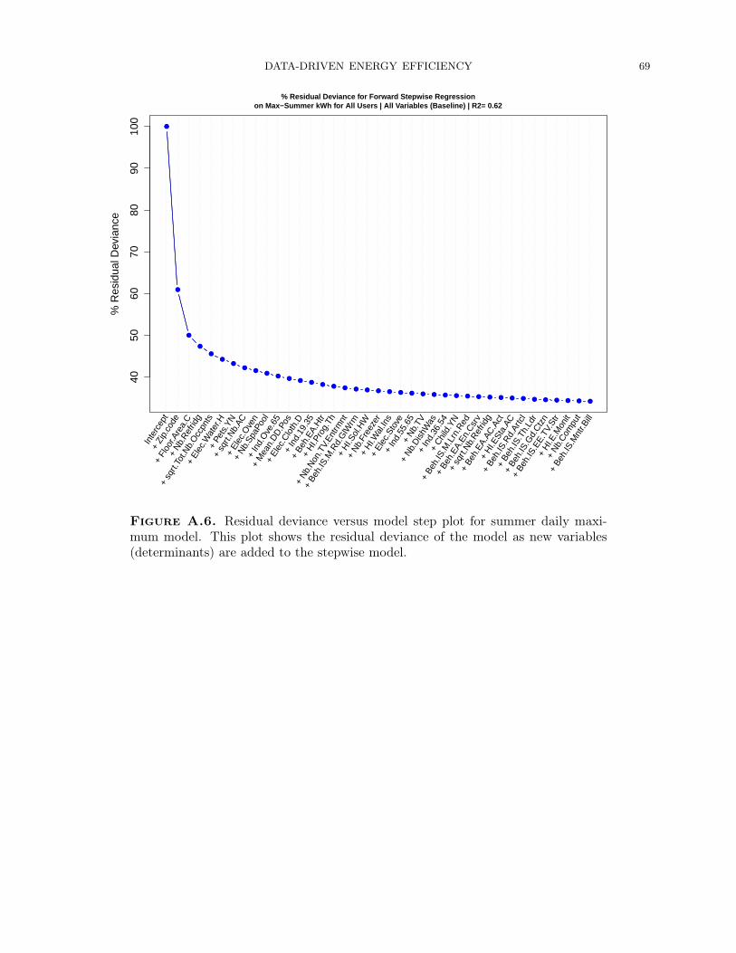
DATA-DRIVEN ENERGY EFFICIENCY 69
●
●
●
●
●
●●
●●
●●
●● ●
● ● ● ● ● ● ● ● ● ● ● ● ● ● ● ● ● ● ● ● ● ● ● ● ●
4050
6070
8090
100
% Residual Deviance for Forward Stepwise Regressionon Max−Summer kWh for All Users | All Variables (Baseline) | R2= 0.62
% R
esid
ual D
evia
nce
Inte
rcep
t+
Zip.
code
+ Fl
oor.A
rea.
C
+ N
b.R
efrid
g
+ sq
rt.To
t.Nb.
Occ
pnts
+ El
ec.W
ater
.H+
Pets
.YN
+ sq
rt.N
b.AC
+ El
ec.O
ven
+ N
b.Sp
aPoo
l
+ In
d.O
ve.6
5
+ M
ean.
DD
.Pos
+ El
ec.C
loth
.D+
Ind.
19.3
5
+ Be
h.EA
.Htr
+ H
I.Pro
g.Th
+ N
b.N
on.T
V.En
trmnt
+ Be
h.IS
.M.R
d.G
lWrm
+ H
I.Sol
.HW
+ N
b.Fr
eeze
r
+ H
I.Wal
.Ins
+ El
ec.S
tove
+ In
d.55
.65
+ N
b.TV
+ N
b.D
ishW
as+
Ind.
36.5
4+
Chi
ld.Y
N
+ Be
h.IS
.M.L
rn.R
ed
+ Be
h.EA
.En.
Csr
v
+ sq
rt.N
b.R
efrid
g
+ Be
h.EA
.AC
.Act
+ H
I.ESt
a.AC
+ Be
h.IS
.Rd.
Artc
l
+ Be
h.IS
.Th.
Ldr
+ Be
h.IS
.Gd.
Ctz
n
+ Be
h.IS
.EE.
TV.S
tr
+ H
I.E.M
onit
+ N
b.C
ompu
t
+ Be
h.IS
.Mnt
r.Bill
●
●
●
●
●●
●●
●●
● ● ● ● ● ● ● ● ● ● ● ● ● ● ● ● ● ● ● ● ● ● ● ● ● ● ● ● ●
Figure A.6. Residual deviance versus model step plot for summer daily maxi-mum model. This plot shows the residual deviance of the model as new variables(determinants) are added to the stepwise model.
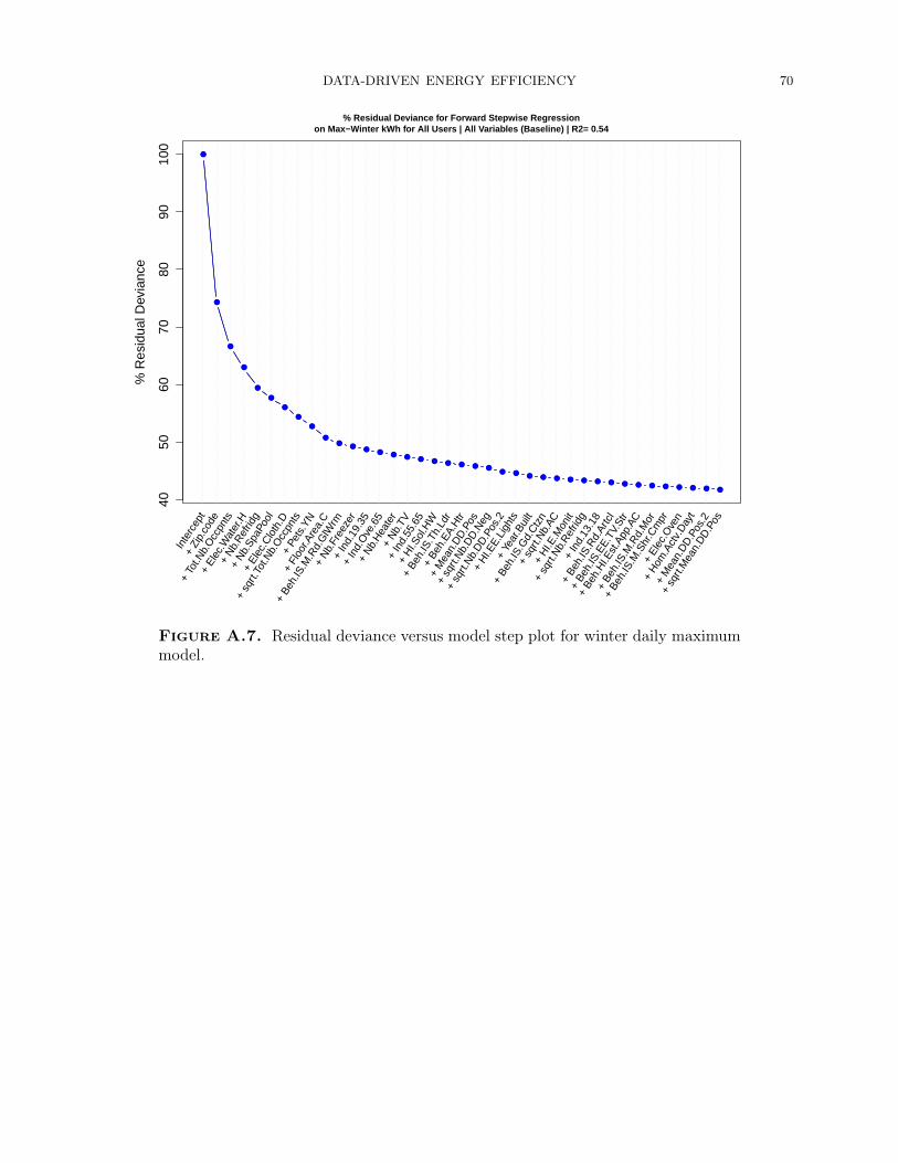
DATA-DRIVEN ENERGY EFFICIENCY 70
●
●
●
●
●
●
●
●
●
●●
●●
●● ● ● ● ● ● ● ●
● ●● ● ● ● ● ● ● ● ● ● ● ● ● ● ●
4050
6070
8090
100
% Residual Deviance for Forward Stepwise Regressionon Max−Winter kWh for All Users | All Variables (Baseline) | R2= 0.54
% R
esid
ual D
evia
nce
Inte
rcep
t+
Zip.
code
+ To
t.Nb.
Occ
pnts
+ El
ec.W
ater
.H
+ N
b.R
efrid
g
+ N
b.Sp
aPoo
l
+ El
ec.C
loth
.D
+ sq
rt.To
t.Nb.
Occ
pnts
+ Pe
ts.Y
N
+ Fl
oor.A
rea.
C
+ Be
h.IS
.M.R
d.G
lWrm
+ N
b.Fr
eeze
r+
Ind.
19.3
5
+ In
d.O
ve.6
5
+ N
b.H
eate
r+
Nb.
TV+
Ind.
55.6
5
+ H
I.Sol
.HW
+ Be
h.IS
.Th.
Ldr
+ Be
h.EA
.Htr
+ M
ean.
DD
.Pos
+ sq
rt.N
b.D
D.N
eg
+ sq
rt.N
b.D
D.P
os.2
+ H
I.EE.
Ligh
ts+
Year
.Bui
lt
+ Be
h.IS
.Gd.
Ctz
n
+ sq
rt.N
b.AC
+ H
I.E.M
onit
+ sq
rt.N
b.R
efrid
g+
Ind.
13.1
8
+ Be
h.IS
.Rd.
Artc
l
+ Be
h.IS
.EE.
TV.S
tr
+ Be
h.H
I.Est
.App
.AC
+ Be
h.IS
.M.R
d.M
or
+ Be
h.IS
.M.S
hr.C
mpr
+ El
ec.O
ven
+ H
om.A
ctv.
Day
t
+ M
ean.
DD
.Pos
.2
+ sq
rt.M
ean.
DD
.Pos
●
●
●
●
●
●
●
●
●
●●
●● ● ● ● ● ● ● ● ● ●
● ● ● ● ● ● ● ● ● ● ● ● ● ● ● ● ●
Figure A.7. Residual deviance versus model step plot for winter daily maximummodel.

DATA-DRIVEN ENERGY EFFICIENCY 71
●
●
●
●
●
●●
●●
●●
● ● ● ● ● ● ● ● ● ● ● ● ● ● ● ● ● ● ● ● ● ● ● ● ● ● ●4050
6070
8090
100
% Residual Deviance for Forward Stepwise Regressionon Max−Min−Summer kWh for All Users | All Variables (Baseline) | R2= 0.57
% R
esid
ual D
evia
nce
Inte
rcep
t+
Zip.
code
+ Fl
oor.A
rea.
C
+ sq
rt.To
t.Nb.
Occ
pnts
+ El
ec.W
ater
.H
+ N
b.R
efrid
g
+ sq
rt.N
b.AC
+ El
ec.C
loth
.D
+ In
d.O
ve.6
5
+ N
b.Sp
aPoo
l
+ N
b.F.
T.Em
p
+ M
ean.
DD
.Pos
+ El
ec.S
tove
+ H
I.Pro
g.Th
+ Pe
ts.Y
N
+ N
b.D
ishW
as
+ H
I.Sol
.HW
+ Be
h.EA
.Htr
+ H
I.Wal
.Ins
+ In
d.6.
12
+ Be
h.IS
.Gd.
Ctz
n
+ Be
h.IS
.M.L
rn.R
ed
+ Be
h.IS
.EE.
TV.S
tr
+ Be
h.IS
.Rd.
Artc
l
+ Be
h.EA
.AC
.Act
+ H
I.E.M
onit
+ Be
h.IS
.Th.
Ldr
+ In
d.19
.35
+ In
d.55
.65
+ C
hild
.YN
+ H
I.ESt
a.AC
+ N
b.H
eate
r
+ N
b.N
on.T
V.En
trmnt
+ sq
rt.N
b.R
efrid
g+
Year
.Bui
lt
+ Be
h.EA
.En.
Csr
v+
Ind.
36.5
4
+ H
om.A
ctv.
Day
t
●
●
●
●
●
●●
●●
●●
● ● ● ● ● ● ● ● ● ● ● ● ● ● ● ● ● ● ● ● ● ● ● ● ● ● ●
Figure A.8. Residual deviance versus model step plot for summer daily maximumminus minimum model. This plot shows the residual deviance of the model as newvariables (determinants) are added to the model. Daily maximum - minimum modelis very similar to the daily maximum model, but it highlights occupants’ variableseven more because the effect of the longer-term structural determinants (locationand building) is removed by subtracting the daily minimum. The summer model,even in the presence of zip code and floor area, now includes Number of Occupants,Ownership of Electric Water Heater, and Number of Refrigerators. Whenzip code and floor area are excluded from the summer model, temperature vari-ables and high-consumption variables increase in rank. The winter model showsthe relationship between maximum load and number of occupants more explicitly:only the square root of number of occupants appears in the model, implyingthat the daily maximum has an inverse quadratic relationship with the number ofoccupants. This means if the number of occupants is doubled, the daily maximumis increased by a factor less than 2, because some of the energy end uses are sharedby the occupants.

DATA-DRIVEN ENERGY EFFICIENCY 72
●
●
●
●
●
●
●
●●
●●
●●
● ● ● ● ● ● ● ● ● ● ●●
● ● ● ● ● ● ● ● ● ● ●
5060
7080
9010
0
% Residual Deviance for Forward Stepwise Regressionon Max−Min−Winter kWh for All Users | All Variables (Baseline) | R2= 0.48
% R
esid
ual D
evia
nce
Inte
rcep
t+
Zip.
code
+ sq
rt.To
t.Nb.
Occ
pnts
+ El
ec.W
ater
.H
+ N
b.R
efrid
g
+ El
ec.C
loth
.D
+ N
b.Sp
aPoo
l+
Pets
.YN
+ N
b.H
eate
r
+ In
d.O
ve.6
5+
Ind.
19.3
5
+ Be
h.IS
.Frc
st.S
v
+ Be
h.IS
.M.R
d.M
or+
HI.C
aulk
+ H
I.EE.
Ligh
ts
+ sq
rt.N
b.R
efrid
g+
Nb.
TV+
Ind.
55.6
5
+ H
I.Sol
.HW
+ Be
h.IS
.Th.
Ldr
+ H
I.E.M
onit
+ Be
h.IS
.M.R
d.G
lWrm
+ M
ean.
DD
.Pos
+ sq
rt.N
b.D
D.N
eg
+ sq
rt.N
b.D
D.P
os.2
+ Ye
ar.B
uilt
+ N
b.Fr
eeze
r
+ sq
rt.N
b.AC
+ Be
h.IS
.Rd.
Artc
l
+ Be
h.IS
.EE.
TV.S
tr
+ H
om.A
ctv.
Day
t+
Ind.
Und
.5
+ N
b.D
ishW
as
+ N
b.H
eate
r.2
+ Be
h.IS
.Lrn
.Cns
.Imp
+ Be
h.EA
.Off.
Cm
p.Pw
r
●
●
●
●
●
●
●
●●
●● ●
● ● ● ● ● ● ● ● ● ● ● ●●
● ● ● ● ● ● ● ● ● ● ●
Figure A.9. Residual deviance versus model step plot for winter daily maximumminus minimum model.