CIE TN 006:2016files.cie.co.at/883_CIE_TN_006-2016.pdf · TECHNICAL NOTE . Visual Aspects of...

TECHNICAL NOTE

Visual Aspects of Time-Modulated Lighting Systems – Definitions and Measurement Models

CIE TN 006:2016

CIE TN 006:2016

II CIE, All rights reserved.

CIE Technical Notes (TN) are short technical papers summarizing information of fundamental importance to CIE Members and other stakeholders, which either have been prepared by a TC, in which case they will usually form only a part of the outputs from that TC, or through the auspices of a Reportership established for the purpose in response to a need identified by a Division or Divisions.

This Technical Note has been prepared by CIE Technical Committee 1-83 of Division 1 “Vision and Colour" and has been approved by the Board of Administration as well as by Division 1 of the Commission Internationale de l'Eclairage. The document reports on current knowledge and experience within the specific field of light and lighting described, and is intended to be used by the CIE membership and other interested parties. It should be noted, however, that the status of this document is advisory and not mandatory.

Any mention of organizations or products does not imply endorsement by the CIE. Whilst every care has been taken in the compilation of any lists, up to the time of going to press, these may not be comprehensive.

CIE 2016 - All rights reserved

CIE TN 006:2016

CIE, All rights reserved. III

The following members of TC 1-83 “Visual Aspects of Time-Modulated Lighting Systems“ took part in the preparation of this Technical Note. The committee comes under Division 1 “Vision and Colour”.

Sekulovski, D. (Chair) Netherlands

Chou, P.-T. Chinese Taipei Couzin, D. Germany Dakin, J. USA Itoh, N. Japan Lee, C.-S. Korea Lee, T.-X. Chinese Taipei Perz, M. Netherlands Pong, A.B.-J. Chinese Taipei Poplawski, M. USA Vogels, I. Netherlands Wang, L. China Whitehead, L. Canada Wilkins, A. United Kingdom Yamauchi, Y. Japan

CIE TN 006:2016

IV CIE, All rights reserved.

CONTENTS

Summary ................................................................................................................................1 1 Introduction .......................................................................................................................2

1.1 Background ...............................................................................................................2 1.2 Scope .......................................................................................................................3 1.3 Structure of the document .........................................................................................4

2 Terms, definitions and fundamentals .................................................................................5 2.1 Introduction ...............................................................................................................5 2.2 Physical characteristics of time-modulated lighting systems ......................................5

2.2.1 Waveform .......................................................................................................5 2.2.2 Time characteristics .......................................................................................5 2.2.3 Intensity characteristics ..................................................................................6 2.2.4 Spatial characteristics ....................................................................................6

2.3 Visibility aspects of time-modulated light ...................................................................7 2.4 General definitions ....................................................................................................7

3 Literature overview ............................................................................................................8 3.1 Fundamental studies and models ..............................................................................8 3.2 Standardized measures to predict visibility of temporal light artefacts .......................9

4 Methodologies for quantification of visibility of temporal light artefacts ............................ 11 4.1 Introduction ............................................................................................................. 11 4.2 Capturing the waveform .......................................................................................... 11

4.2.1 Linearity and sensitivity ................................................................................ 11 4.2.2 Sampling frequency and sample duration ..................................................... 11 4.2.3 Measurement resolution ............................................................................... 11 4.2.4 Normalization of the data ............................................................................. 12

4.3 Frequency domain analysis ..................................................................................... 12 4.3.1 Discrete Fourier transform ............................................................................ 12 4.3.2 Sensitivity normalization ............................................................................... 12 4.3.3 Visibility measure ......................................................................................... 12 4.3.4 Example embodiments ................................................................................. 13

4.4 Time domain analysis .............................................................................................. 15 4.4.1 Introduction .................................................................................................. 15 4.4.2 Temporal filtering ......................................................................................... 16 4.4.3 Computing short-term variance and adjustment ............................................ 16 4.4.4 Statistical processing ................................................................................... 16 4.4.5 Example embodiment ................................................................................... 16

5 Recommendations and future work .................................................................................. 17 References ........................................................................................................................... 17

CIE TN 006:2016

CIE, All rights reserved. 1

Summary

The fast rate at which solid state light sources can change their intensity is one of the main drivers behind the revolution in the lighting world and applications of lighting. Linked to the fast rate of the intensity change is a direct transfer of the modulation of the driving current, both intended and unintended, to a modulation of the luminous output. In turn, the light modulation can give rise to changes in the perception of the environment. While in some very specific entertainment applications a change of perception due to light modulation is desired, for most everyday applications and activities the change is detrimental and undesired. These changes in the perception of the environment are called “temporal light artefacts” (TLAs) and can have a large influence on the judgment of the light quality. Moreover, the visible modulation of light can lead to a decrease in performance, increased fatigue as well as acute health problems like epileptic seizures and migraine episodes.

The potential negative impact of temporal light artefacts has prompted lighting manufacturers, lighting application specialists, universities and governments to look for ways to measure the impact and come to a better understanding of the temporal quality aspects of lighting systems. In this context, the CIE formed Technical Committee (TC) 1-83 "Visual Aspects of Time-Modulated Lighting Systems".

This Technical Note (TN) is an intermediate product of the work of the TC. In the first part of the TN, new definitions for the perceptual effects modulated light can produce are given. In the second part, an overview of the relevant literature is given as well as an overview of the parameters that influence the visibility of the different TLAs. The last part gives a description of two methods, one in the time domain and one in the frequency domain, which can be used to quantify TLAs. Furthermore, three implementations of the general methods into specific visibility measures are given as an example.

CIE TN 006:2016

2 CIE, All rights reserved.

1 Introduction

1.1 Background Solid state lighting has revolutionized the world of lighting and lighting applications. The introduction of small, bright light sources which can change intensity at a very high rate and which have an almost arbitrary spectrum has profound influence on lighting quality (Schubert & Kim, 2005; Schubert et al., 2006). While in traditional lighting, the search for optimal light was limited to the capabilities of the technology, the almost limitless capabilities of solid state lighting call for a more fundamental approach, starting from human perception, and not from the hardware limitations.

Some of the technological advantages can introduce perceptible side effects that were either absent or less prominent in traditional lighting systems. One such advantage is the fast reaction of solid state light sources to the driving current. The response time can be as short as a couple of nanoseconds and results in an almost instantaneous translation of the driving current to the luminous output. As the driving current of most electric light sources is modulated, so is the light output intensity and colour. The simplest and most common source of modulation is unintended and results from the supply of the lighting equipment with mains power, usually modulated at 50 Hz or 60 Hz or twice these frequencies through a rectifier. Further modulation can originate from interactions between the driver and dimmer electronics or as a result of disturbances in the mains power induced by other loads on the network.

The fast reaction of solid state light sources is in sharp contrast to the reaction times of previous generations of electric light sources. Incandescent and halogen sources have emissions based on thermal process that are slower than electrical processes. This is evident in the so-called “afterglow” effect of an incandescent lamp being switched off. Fluorescent sources typically use phosphorescent materials with time constants in the order of 200 ms to transfer the UV radiation produced by the mercury vapour into visible radiation. In this case, the slow phosphor acts as an optical low-pass filter on the output of the fluorescent lamp. Metal halide lamps are well known for their inability with respect to temporal modulation. Many of them need more than 30 min after switching off before they can be switched on again.

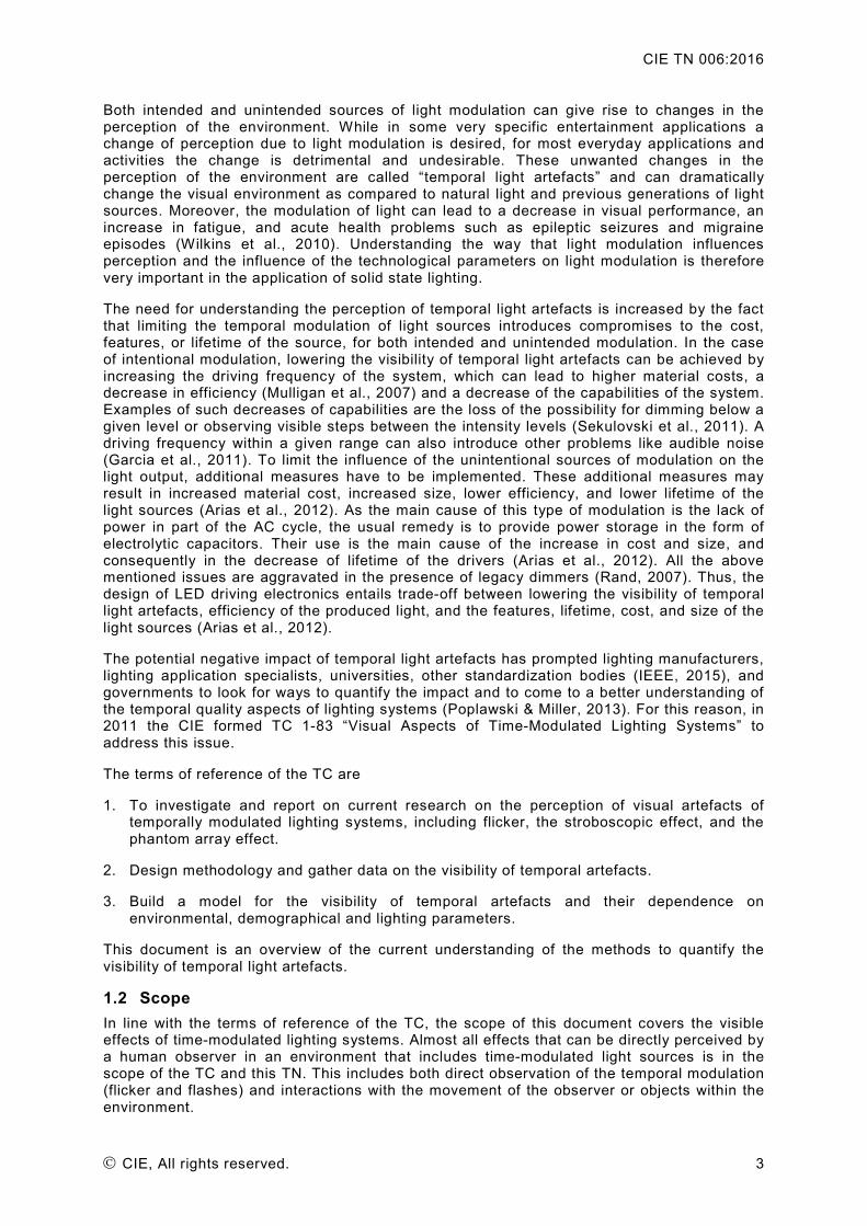
Temporal light modulation can also be intended and is used for control of intensity and colour. Using temporal modulation ensures that the solid state light sources are always driven in a similar operating range and results in simpler, usually linear, models of their behaviour (Pousset et al., 2010). Examples of such driving schemes are pulse width and pulse density modulation, often used in colour-tuneable light sources. Figure 1 below and Figure 2 in Clause 2 depict examples of time-modulated light signals, from unintended modulation arising from AC mains and from intended modulation produced by a system that uses a pulse width modulation scheme, respectively.

Figure 1 – Example of a time-modulated light output (unintended light modulation over time caused by AC mains)

Rel

ativ

e lu

min

ance

Time / s

0 0,02 0,04 0,06 0,08 0,10 0,12 0,14 0,16 0,18 0,20

CIE TN 006:2016


Both intended and unintended sources of light modulation can give rise to changes in the perception of the environment. While in some very specific entertainment applications a change of perception due to light modulation is desired, for most everyday applications and activities the change is detrimental and undesirable. These unwanted changes in the perception of the environment are called “temporal light artefacts” and can dramatically change the visual environment as compared to natural light and previous generations of light sources. Moreover, the modulation of light can lead to a decrease in visual performance, an increase in fatigue, and acute health problems such as epileptic seizures and migraine episodes (Wilkins et al., 2010). Understanding the way that light modulation influences perception and the influence of the technological parameters on light modulation is therefore very important in the application of solid state lighting.

The need for understanding the perception of temporal light artefacts is increased by the fact that limiting the temporal modulation of light sources introduces compromises to the cost, features, or lifetime of the source, for both intended and unintended modulation. In the case of intentional modulation, lowering the visibility of temporal light artefacts can be achieved by increasing the driving frequency of the system, which can lead to higher material costs, a decrease in efficiency (Mulligan et al., 2007) and a decrease of the capabilities of the system. Examples of such decreases of capabilities are the loss of the possibility for dimming below a given level or observing visible steps between the intensity levels (Sekulovski et al., 2011). A driving frequency within a given range can also introduce other problems like audible noise (Garcia et al., 2011). To limit the influence of the unintentional sources of modulation on the light output, additional measures have to be implemented. These additional measures may result in increased material cost, increased size, lower efficiency, and lower lifetime of the light sources (Arias et al., 2012). As the main cause of this type of modulation is the lack of power in part of the AC cycle, the usual remedy is to provide power storage in the form of electrolytic capacitors. Their use is the main cause of the increase in cost and size, and consequently in the decrease of lifetime of the drivers (Arias et al., 2012). All the above mentioned issues are aggravated in the presence of legacy dimmers (Rand, 2007). Thus, the design of LED driving electronics entails trade-off between lowering the visibility of temporal light artefacts, efficiency of the produced light, and the features, lifetime, cost, and size of the light sources (Arias et al., 2012).

The potential negative impact of temporal light artefacts has prompted lighting manufacturers, lighting application specialists, universities, other standardization bodies (IEEE, 2015), and governments to look for ways to quantify the impact and to come to a better understanding of the temporal quality aspects of lighting systems (Poplawski & Miller, 2013). For this reason, in 2011 the CIE formed TC 1-83 “Visual Aspects of Time-Modulated Lighting Systems” to address this issue.

The terms of reference of the TC are

1. To investigate and report on current research on the perception of visual artefacts of temporally modulated lighting systems, including flicker, the stroboscopic effect, and the phantom array effect.

2. Design methodology and gather data on the visibility of temporal artefacts.

3. Build a model for the visibility of temporal artefacts and their dependence on environmental, demographical and lighting parameters.

This document is an overview of the current understanding of the methods to quantify the visibility of temporal light artefacts.

1.2 Scope In line with the terms of reference of the TC, the scope of this document covers the visible effects of time-modulated lighting systems. Almost all effects that can be directly perceived by a human observer in an environment that includes time-modulated light sources is in the scope of the TC and this TN. This includes both direct observation of the temporal modulation (flicker and flashes) and interactions with the movement of the observer or objects within the environment.

CIE TN 006:2016


Furthermore the visibility of time-modulated light effects depends on many environmental factors that differ for each application. For those parts of the document which are specific to an application or a set of applications, the applicability will be clearly stated.

To keep the focus of the TC and this TN, the effects described below are not in the scope of this TN.

Modulation schemes that change the spectrum of the light, while maintaining the same luminance, can also give rise to flicker, called “chromatic flicker” or “colour flicker”. However, the chromatic channels of human vision show much lower temporal sensitivity compared to the achromatic channel (Swanson et al., 1987; Perz, 2010). For most lighting systems, luminance flicker is the dominant effect. For this reason, no models that describe the visibility of chromatic flicker will be presented in this TN. The general methods, however, can still be applied using appropriate sensitivity curves.

This TN does not cover so-called flashing light, which consists of time-modulated light at very low frequencies such as 1 Hz and used for beacons and traffic warning lights for increased visibility or conspicuity (this is covered in CIE TC 2-49).

Time-modulated lighting systems might also give rise to non-visual effects among the user population (IEEE, 2015). These effects, however, are outside of the scope of the work of the TC and this TN.

The work of the TC concerns the visibility of the temporal light artefacts. The amount of modulation that is acceptable in an application (beyond the visibility thresholds) depends on the specific application. Acceptable limits to modulation might be more strictly defined by other effects that are not part of this TN. Acceptability thresholds are therefore not within the scope of this TN.

The scope of the work of the TC only includes conditions where a human observer directly interacts with an environment lit by a time-modulated light source. Thus, unwanted artefacts through interactions with capture and reproduction systems such as TV recording, broadcasting and personal video are outside the scope of this work. Interactions with non-human vision, like animal, insect or machine vision are also outside the scope.

1.3 Structure of the document One of the possible sources of confusion in scientific literature, standards and regulations and commercial communication is the absence of standardized terminology for temporal light artefacts with unambiguous meaning. The meaning of the term “flicker” is not clearly defined when used in a different (but even in the same) context. Descriptions range from direct visual observation, through interactions with moving objects and subconscious effects on humans, to being just another term for time-modulated light. One of the early tasks of TC 1-83 was to review the definitions in use today and to propose a new, less ambiguous set of definitions, which are described in Clause 2.

Clause 3 of this document gives a concise overview of relevant literature on the topic. It is by no means complete, but should provide a good starting point.

Depending on the type of modulation that is predominantly present, specific methodologies for analysis are appropriate. On the one hand, periodic modulations that are presented long enough to be perceived and have a well-defined set of frequencies are better suited for frequency domain analysis. On the other hand, aperiodic modulations, transient modulations or modulations with random frequency components are better suited for time domain analysis. Clause 4 discusses both methodologies and gives two general frameworks, in which the effects of both types of modulations can be quantified. Examples of implementations of the framework are included.

Clause 5 formulates recommendations for the methods to be used to quantify the visibility of temporal light artefacts. These recommendations are expected to be updated in a Technical Report that is going to be prepared by the TC. Furthermore, recommendations for future work

CIE TN 006:2016


are given as there is a clear need for validation and extension of the knowledge on the visibility of temporal light artefacts.

2 Terms, definitions and fundamentals

2.1 Introduction Temporal modulation of light can give rise to a number of different temporal light artefacts. This is, however, not represented in the definitions that are currently in use. In some contexts, the term “flicker” is also used to describe temporal modulation of the light itself, whether the light modulation produces visual effects or not. In this TN, the term “temporal modulation” is used for any measurable change of the intensity or the spectral distribution of the light. The term “flicker” is only used for the direct perception of the modulation.

Furthermore, the extent of applicability of the definitions is also not clear, which might lead to ambiguous interpretations. The CIE defines the term “flicker” as:

impression of unsteadiness of visual perception induced by a light stimulus whose luminance or spectral distribution fluctuates with time (CIE, 2011, term 17-443).

This definition clearly defines flicker as a perceptual effect. The extent of applicability is however unclear. Both direct observation of time modulation of light as well as the interaction with movements of the observer or in the environment could be part of this definition, but are not necessarily so. For these reasons, the interpretation of the definition can be ambiguous.

The interpretation of the term “flicker” is mostly connected to direct observation of the time modulation, without consideration of interaction with movements. Because of this, the introduction of a new term, “temporal light artefact” (“TLA”), and a revised definition of “flicker” are proposed. In addition definitions for further terms used in this document are listed in the following clause. For all new terms defined, the respective definitions give the minimal requirements for the detection, but do not limit the visibility to only those conditions. For example, flicker is visible in a static environment, but this does not mean that it is not visible in an environment that has moving objects.

2.2 Physical characteristics of time-modulated lighting systems In this clause, physical characterization of temporally modulated light is discussed and the basic terms used later in the document are described.

2.2.1 Waveform The graph of the variation of a luminous quantity (luminance or luminous intensity) emitted by a light source as a function of time, y(t), is called “light waveform”. In the rest of the document, for brevity, the term “waveform” is used meaning “light waveform”.

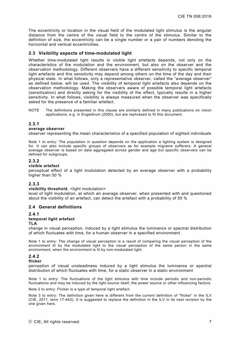
A repetitive waveform is a waveform that is equal to all shifted versions of itself by an integer multiple, k, of a fixed time, T, i.e. y(t) = y(t + kT). An example of a square time modulation, a common repetitive waveform, is given in Figure 2.

In most practical applications, waveforms are represented by their digitized version, with a discretized representation of both time and intensity. Non-repetitive waveforms cannot be represented with a finite time sample and are typically approximated by a limited time digitized version.

2.2.2 Time characteristics The period of the repetitive waveform is denoted T, and its reciprocal, the frequency, is denoted f. For a single cycle of a repetitive waveform, the time for which the intensity is above 10 % of the maximum intensity of the waveform is called the active period, Ta . The ratio of the active period to the period of a waveform is called a duty cycle, D, and can vary from 0 to 1. The duty cycle is usually used to describe square waveform modulations (Figure 2).

CIE TN 006:2016


Figure 2 – Square modulation of light

2.2.3 Intensity characteristics Within a period of time, a waveform reaches a maximum intensity, y max, and a minimum intensity, ymin , and has a time average, y . Modulation depth (symbol DM

1) is defined as

max minM

max min

y yDy y

−=

+ (1)

For waveforms for which the time-average, y , is equal to max min)( ) / 2y y+ , the modulation

depth is equal to: M max min)( ) / (2 )D y y y= − . Modulation depth is often expressed as a percentage.

2.2.4 Spatial characteristics Depending on the application, the time-modulated part of the visual field can vary in its spatial layout, complexity and relation to the non-modulated part of the visual field. A number of descriptors of the spatial characteristics of modulated light will be defined below using a simple example layout. This simple case contains a single modulated part of the visual field (possibly with spatially non-uniform luminance) surrounded by a spatially uniform non-modulated background. The modulated and non-modulated parts of the visual field are called the modulated light stimulus and the background, respectively. The modulated light stimulus is also known as the test field.

The contrast (Weber contrast), CM, of the modulated light stimulus is defined as

s bM

b

L LCL−

= (2)

Where sL is the (space and time) average of the modulated stimulus luminance, and Lb is the luminance of the background. Note that the Weber contrast can be negative as the average luminance of the modulated light can be lower than the background. An example of negative contrast is a display with a modulated backlight in front of a wall with a higher luminance.

The visual size of the modulated stimulus is the angular extent of the modulated stimulus having an absolute value of the contrast that exceeds 10 % of the maximum absolute value of the contrast. The visual size can be a single number, as in the case of a circularly symmetric modulated light stimulus, or a pair of numbers denoting the horizontal and vertical size. ————————— 1 Note that the abbreviation of the term “modulation depth”, MD, is often used as quantity symbol, too. This does

not conform with the CIE rules and the rules of other standardizing organizations regarding the presentation of quantity symbols. For that reason the symbol DM is introduced for the quantity “modulation depth” in this document.

0 Ta T T+Ta 2T 2T+Ta 3T 3T+Ta

ymin

ymax

CIE TN 006:2016


The eccentricity or location in the visual field of the modulated light stimulus is the angular distance from the centre of the visual field to the centre of the stimulus. Similar to the definition of size, the eccentricity can be a single number or a pair of numbers denoting the horizontal and vertical eccentricities.

2.3 Visibility aspects of time-modulated light Whether time-modulated light results in visible light artefacts depends, not only on the characteristics of the modulation and the environment, but also on the observer and the observation methodology. Different observers have a different sensitivity to specific temporal light artefacts and this sensitivity may depend among others on the time of the day and their physical state. In what follows, only a representative observer, called the “average observer” as defined below, will be used. The visibility of temporal light artefacts also depends on the observation methodology. Making the observers aware of possible temporal light artefacts (sensitization) and directly asking for the visibility of the effect, typically results in a higher sensitivity. In what follows, visibility is always measured when the observer was specifically asked for the presence of a familiar artefact.

NOTE The definitions presented in this clause are similarly defined in many publications on vision applications, e.g. in Engeldrum (2000), but are rephrased to fit this document.

2.3.1 average observer observer representing the mean characteristics of a specified population of sighted individuals

Note 1 to entry: The population in question depends on the application a lighting system is designed for. It can also include specific groups of observers as for example migraine sufferers. A general average observer is based on data aggregated across gender and age but specific observers can be defined for subgroups.

2.3.2 visible artefact perceptual effect of a light modulation detected by an average observer with a probability higher than 50 %

2.3.3 visibility threshold, <light modulation> level of light modulation, at which an average observer, when presented with and questioned about the visibility of an artefact, can detect the artefact with a probability of 50 %

2.4 General definitions 2.4.1 temporal light artefact TLA change in visual perception, induced by a light stimulus the luminance or spectral distribution of which fluctuates with time, for a human observer in a specified environment

Note 1 to entry: The change of visual perception is a result of comparing the visual perception of the environment lit by the modulated light to the visual perception of the same person in the same environment, when the environment is lit by non-modulated light.

2.4.2 flicker perception of visual unsteadiness induced by a light stimulus the luminance or spectral distribution of which fluctuates with time, for a static observer in a static environment

Note 1 to entry: The fluctuations of the light stimulus with time include periodic and non-periodic fluctuations and may be induced by the light source itself, the power source or other influencing factors.

Note 2 to entry: Flicker is a type of temporal light artefact.

Note 3 to entry: The definition given here is different from the current definition of “flicker” in the ILV (CIE, 2011, term 17-443). It is suggested to replace the definition in the ILV in its next revision by the one given here.

CIE TN 006:2016


2.4.3 stroboscopic effect change in motion perception induced by a light stimulus the luminance or spectral distribution of which fluctuates with time, for a static observer in a non-static environment

Note 1 to entry: The stroboscopic effect is a type of temporal light artefact.

EXAMPLE 1 For a square periodic luminance fluctuation, moving objects are perceived to move discretely rather than continuously.

EXAMPLE 2 If the frequency of a periodic luminance fluctuation coincides with the frequency of a rotating object, the rotating object is perceived as static.

2.4.4 phantom array effect ghosting change in perceived shape or spatial positions of objects, induced by a light stimulus the luminance or spectral distribution of which fluctuates with time, for a non-static observer in a static environment

Note 1 to entry: The phantom array effect is a type of temporal light artefact.

EXAMPLE When making a saccade over a small light source having a square periodic luminance fluctuation, the light source is perceived as a series of spatially extended light spots.

2.4.5 static observer observer who does not move her/his eye(s)

Note 1 to entry: Only large eye movements (saccades) fall under this definition. An observer that only does involuntary micro-saccades is considered static.

2.4.6 static environment environment that does not contain perceivable motion under non-modulated lighting conditions

3 Literature overview

3.1 Fundamental studies and models The topic of the visibility of temporal light modulation is not a new one. The most studied temporal light artefact, flicker, has been a topic of considerable interest in the literature.

Early works on flicker mention specific forms of time modulation, like flashes or ramps, and determined the relationship between the parameters of those particular forms of time modulation and the perceived effect. A number of results are known as perceptual laws, including Bloch’s law (Watson, 1986), the Ferry-Porter law (Watson, 1986), and the Granit-Harper law (Hecht & Shlaer, 1936). Early works using repetitive modulation concentrated on the parameters that affect the highest modulation frequency still visible as flicker, known as the critical flicker fusion (CFF) threshold, also called “flicker fusion frequency”.

After 1950, a more general approach based on linear systems theory was introduced to visual perception by De Lange (1958; 1961) and Kelly (1959; 1961). In the subsequent work, flicker visibility has been shown to depend on many quantities, including the temporal frequency of the light changes, the magnitude of change, the shape of the waveform, the light intensity, the position in the visual field (Tyler, 1987; Tyler & Hamer, 1990; Perz, 2010) and the spatial extent of the modulated light, and the adaptation state of the observer. To characterize the visibility of flicker due to temporal modulations using the linear systems approach, a temporal contrast sensitivity function (TCSF) is used. It is obtained by measuring the contrast sensitivity to sinusoidal stimuli for a number of frequencies. Contrast sensitivity is the reciprocal of the visibility threshold, defined as the modulation depth (see Equation (1)) at which an average observer can detect flicker with a probability of 50 %. As with other

CIE TN 006:2016


perceptual correlates, the human visual system also adapts to flicker (Shady et al., 2004). Thus, the sensitivity for flicker is attenuated after prolonged exposure to a flickering stimulus.

De Lange gave the basis for prediction of visibility of flicker for complex stimuli (De Lange, 1961) by demonstrating that the visibility of all the waveforms depended on the amplitude at the fundamental frequency. Levinson (1960) demonstrated that for waveforms where additional frequencies have amplitudes that result in similar visibility of the harmonics to the fundamental frequency, all frequencies have to be taken into account. Furthermore Levinson demonstrated that under specific conditions there is also an influence of the relative phase between multiple frequency components. Recent work on modelling of flicker of lighting systems (Perz et al., 2013; Bodington et al., 2015) used similar methodologies and supported the findings of Levinson in the target applications. Additionally, both Perz et al. and Bodington et al. used a general Minkowski summation procedure (Shepard, 1987) to account for the interaction of multiple frequencies.

The next step in the development of flicker visibility measures was to do the analysis in the time domain. A number of approaches to determine the time domain filters needed are described in literature. One line of research used assumptions of minimal phase (Kelly, 1971; Swanson et al., 1987; Stork & Falk, 1987), but Tyler (1992) showed that minimum phase assumption was not compatible with results from psychophysics. Another line of research used physiologically inspired parametric models (Ikeda & Boynton, 1965; Roufs, 1972; Roufs & Blommaert, 1981; Watson, 1982). Watson (1986) and Ikeda (1986) are recommended sources for a review on the topic. Rashbass (1970) used a two-flash methodology to develop a technique that is used as a basis for the most established flicker quantification method, the IEC Flickermeter (IEC, 2010).

Flicker is perceived up to frequencies of ~80 Hz depending on the conditions. The stroboscopic effect, on the contrary, may also occur for light fluctuating with frequencies higher than 100 Hz. Contrary to the rich literature on flicker, literature on the stroboscopic effect is scarcer. The qualitative perception of the stroboscopic effect was studied using different activities and conditions demonstrating that extreme modulation above 100 Hz is deemed unacceptable (Frier & Henderson, 1973; Rea & Ouellette, 1988; Bullough et al., 2011; Vogels et al., 2011). The visibility of the stroboscopic effect depends on the frequency, modulation depth, duty cycle, waveform, spatial contrast of the moving object and background as well as the speed of movement of the objects in the environment (Bullough et al., 2011; Vogels et al., 2011; Perz et al., 2014). To encompass the most important effects on the visibility of the stroboscopic effect, a new measure called the “stroboscopic effect visibility measure” (SVM) was developed (Perz et al., 2014). It is based on Minkowski summation with an exponent of 3,7 and experiments show that the new measure successfully predicts the visibility of single and multiple sinusoids, square waveforms with different duty cycles and real world waveforms (Perz et al., 2014).

Another temporal light artefact that is caused by fluctuating light is the phantom array effect (also known as ghosting). It occurs when a saccade (a movement of the eye) is made across a contour with a sufficiently large contrast that is fluctuating in intensity. The contour is then perceived as a spatially extended series of contours. Roberts and Wilkins (2013) showed that the phantom array effect enabled observers to discriminate modulated from steady light under two alternative forced choice conditions at frequencies up to 2 500 Hz.

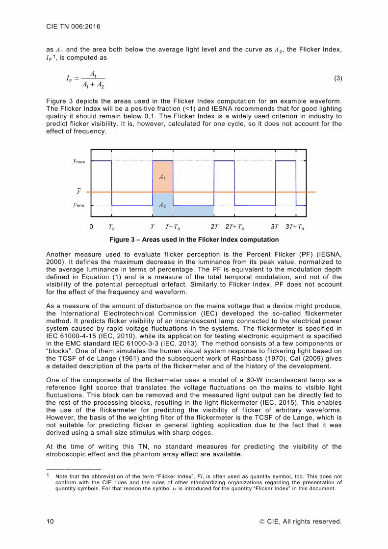
3.2 Standardized measures to predict visibility of temporal light artefacts A number of measures to quantify flicker visibility have been proposed. The Illuminating Engineering Society of North America (IESNA) has defined the Flicker Index (FI) (IESNA, 2000). It is defined as the area between the curve representing the waveform and the average light level divided by the total area below the curve for a single cycle of the fluctuation. Denoting the area between the curve representing the waveform and the average light level

CIE TN 006:2016


as A1 and the area both below the average light level and the curve as A2 , the Flicker Index, IF

1, is computed as

1F

1 2

AIA A

=+

(3)

Figure 3 depicts the areas used in the Flicker Index computation for an example waveform. The Flicker Index will be a positive fraction (<1) and IESNA recommends that for good lighting quality it should remain below 0,1. The Flicker Index is a widely used criterion in industry to predict flicker visibility. It is, however, calculated for one cycle, so it does not account for the effect of frequency.

Figure 3 – Areas used in the Flicker Index computation

Another measure used to evaluate flicker perception is the Percent Flicker (PF) (IESNA, 2000). It defines the maximum decrease in the luminance from its peak value, normalized to the average luminance in terms of percentage. The PF is equivalent to the modulation depth defined in Equation (1) and is a measure of the total temporal modulation, and not of the visibility of the potential perceptual artefact. Similarly to Flicker Index, PF does not account for the effect of the frequency and waveform.

As a measure of the amount of disturbance on the mains voltage that a device might produce, the International Electrotechnical Commission (IEC) developed the so-called flickermeter method. It predicts flicker visibility of an incandescent lamp connected to the electrical power system caused by rapid voltage fluctuations in the systems. The flickermeter is specified in IEC 61000-4-15 (IEC, 2010), while its application for testing electronic equipment is specified in the EMC standard IEC 61000-3-3 (IEC, 2013). The method consists of a few components or “blocks”. One of them simulates the human visual system response to flickering light based on the TCSF of de Lange (1961) and the subsequent work of Rashbass (1970). Cai (2009) gives a detailed description of the parts of the flickermeter and of the history of the development.

One of the components of the flickermeter uses a model of a 60-W incandescent lamp as a reference light source that translates the voltage fluctuations on the mains to visible light fluctuations. This block can be removed and the measured light output can be directly fed to the rest of the processing blocks, resulting in the light flickermeter (IEC, 2015). This enables the use of the flickermeter for predicting the visibility of flicker of arbitrary waveforms. However, the basis of the weighting filter of the flickermeter is the TCSF of de Lange, which is not suitable for predicting flicker in general lighting application due to the fact that it was derived using a small size stimulus with sharp edges.

At the time of writing this TN, no standard measures for predicting the visibility of the stroboscopic effect and the phantom array effect are available.

————————— 1 Note that the abbreviation of the term “Flicker Index”, FI, is often used as quantity symbol, too. This does not

conform with the CIE rules and the rules of other standardizing organizations regarding the presentation of quantity symbols. For that reason the symbol IF is introduced for the quantity “Flicker Index” in this document.

ymax

ymin

A1

0 Ta T T+Ta 2T 2T+Ta 3T 3T+Ta

A2

CIE TN 006:2016


4 Methodologies for quantification of visibility of temporal light artefacts

4.1 Introduction In this clause recommendations for general methods to quantify the visibility of temporal light artefacts will be formulated, based on the literature review. Depending on the type of modulation that is predominantly present, specific analysis methodologies are appropriate. On the one hand, periodic modulations that are presented long enough to be perceived and that have a well-defined set of frequencies, are better suited for frequency domain analysis. On the other hand, aperiodic modulations, transient modulations or modulations with random frequency components are better suited for time domain analysis. In this clause, an overview of the general frameworks which can be used to quantify temporal light artefacts in the frequency and time domain are given. Furthermore, examples of implementations of these general frameworks in specific contexts are given.

Both approaches have two things in common: First, they both start with capturing and digitization of the waveform. Second, they both result in a single number that quantifies visibility where a value of 1 corresponds to modulation at visibility threshold.

4.2 Capturing the waveform Translating the luminance modulation over time to a digital signal that can be further analysed is a challenging problem in the general case. The details of the system and the procedure of capturing are beyond the scope of this TN. However, a number of requirements have to be fulfilled for the capture to be suitable for the quantification of the luminous temporal light artefacts.

4.2.1 Linearity and sensitivity The combination of the photo detector, the amplifier and the analogue-to-digital converter has to give a linear response to changes in intensity of the light over the required frequency range. In the cases where only the relative intensity change is needed and there is no spectral change in the light output, the spectral sensitivity of the photo detector does not necessarily need to correspond to human spectral sensitivity (CIE, 2004). In case a luminance measurement is needed or there are changes in the spectrum of the stimulus, standard photometric CIE recommendations for the spectral sensitivity of the photo detector should be followed (CIE, 2015).

4.2.2 Sampling frequency and sample duration For periodic waveforms, the highest and the lowest frequency of a luminous modulation that can result in visible temporal light artefacts determine the sampling frequency and the sample duration needed for the quantification. For aperiodic waveforms where statistical processing is used, the probability of detecting an artefact per time unit also influences the sample duration.

For the quantification of flicker, the capture guidelines for the use of the light flickermeter given by IEC (IEC, 2015) should be followed.

The stroboscopic effect and the phantom array effect from periodic waveforms can be seen up to frequencies of 2,5 kHz. Even though they are visible below 80 Hz, the most noticeable effect in that frequency range is flicker. For this reason, the minimum recommended sampling frequency is 20 kHz with a sample duration of one second (minimum) to be able to verify the periodicity of the waveform. The sample duration should be such that the sample has an integer number of periods of the waveform.

4.2.3 Measurement resolution For frequencies between 10 Hz and 20 Hz, flicker can be perceived for modulation depths of less than 0,3 %. The system should be able to measure modulations of this size reliably. It is recommended that at least a 12-bit analogue-to-digital converter is used, which provides 0.025 % resolution in full scale). Furthermore, the noise level of the detector and the amplifier should be low enough for a reliable measurement of such modulations.

CIE TN 006:2016


4.2.4 Normalization of the data The measures found in literature that use frequency domain analysis are developed with a particular application or set of applications in mind. The range of average light levels used in the experiments referred to in the literature is representative for typical indoor conditions. Similar studies can be performed for outdoor light levels. This means that the absolute light intensity is already taken into account in the sensitivity curve that is used, and in this part of the analysis only the relative changes are important. Because of this, as a first step of the process, the waveform is normalized such that the time average equals unity. Normalization is applied to the data in both frequency and time domain analysis.

4.3 Frequency domain analysis For periodic waveforms where the phase information can be neglected, the analysis can be performed in the frequency domain.

4.3.1 Discrete Fourier transform As a first step in the frequency analysis, the time domain digital signal is transferred to a frequency representation using the Discrete Fourier Transform (DFT), usually implemented using the Fast Fourier Transform (FFT) algorithm. After the transform, the amplitudes of the m-th Fourier component are denoted by C m . Due to the normalization steps, these amplitudes are independent of the average light level. Depending on the duration of the signal, the m-th Fourier component will correspond to a given frequency, fm .

The computed amplitudes of real world measured signals can strongly depend on the phase difference between the beginning and the end of the sampling. For a more reliable amplitude estimation it is recommended to apply windowing (by e.g. a Hanning window) before the DFT, follow the DFT by peak finding, and only take the peaks with at least 1 Hz difference as the amplitudes, C m , of the components.

4.3.2 Sensitivity normalization Next, the frequency representation is normalized using the visibility threshold data determined using simple sinusoidal modulations. The normalization is performed by dividing each amplitude, Cm , by the visibility threshold for sinusoidal modulations at the corresponding frequency, Tv(fm). In the following, Tm will be used as a short hand notation for T v(fm ). This normalization takes into account the two most important parameters for the visibility of temporal light artefacts: the frequency and the amplitude at that frequency. Other parameters that do not typically change for an application but might change between different contexts can be taken into account by selecting an appropriate sensitivity curve. For each specific embodiment of the general framework, the range of applicability corresponding to the sensitivity curve used should be clearly specified.

For both the flicker and the stroboscopic effect, studies have shown that in modulations consisting of multiple frequencies close to their respective visibility thresholds, all these frequencies contribute to the visibility of the overall modulation. Reports from literature also show that the frequency summation can be different for different artefacts. To allow for the difference in summation of the modulations for different frequencies, a general Minkowski norm Ln is used (Shepard, 1987). By varying the exponent, n, a number of different norms are produced. Setting n = 2 results in the standard Euclidean norm, used by Bodington et al. (2015) and Perz et al. (2013) for their quantification of flicker, while setting the limit n → ∞ results in the Chebyshev norm, used by De Lange (1958) for his quantification of flicker.

4.3.3 Visibility measure Taking the steps described above, the input modulation is translated into a single number, which conveniently quantifies the visibility of the temporal light artefact. The corresponding

CIE TN 006:2016


quantity is called “visibility measure” (symbol M v1) and can be calculated with the following

equation:

1

v1

n n

m

m m

CMT

∞

=

= ∑ (4)

where C m is the amplitude of the m-th Fourier component and T m is the visibility threshold for the effect for a sine wave at the frequency of the m-th Fourier component. The parameter n is the Minkowski norm parameter, for which examples are provided in 4.3.4. The value of the parameter n can be determined theoretically or based on experimental data. The summation is carried over all the components of the signal with corresponding frequencies that have a defined visibility threshold, Tm , for the sensitivity curve used. For simplicity of notation, the summation in Equation (4) is done over all normalized amplitudes. Outside of the frequency range in which the visibility threshold curve is defined, the normalized amplitudes should be set to zero. If the value of the visibility measure equals to one, the input modulation produces a temporal light artefact that is just visible, i.e. at visibility threshold. This means that an average observer will be able to detect the artefact with a probability of 50 %. If the value of the visibility measure is above unity, the effect has a probability of detection of more than 50 %. If the value of the visibility measure is smaller than unity, the probability of detection is less than 50 %. These visibility thresholds show average detection of an average human observer in a population. This does not, however, guarantee acceptability. For some less critical applications, the acceptability level of an artefact might be well above the visibility threshold. For other applications and artefacts that are more critical such as flicker, the acceptable levels might be below the visibility threshold.

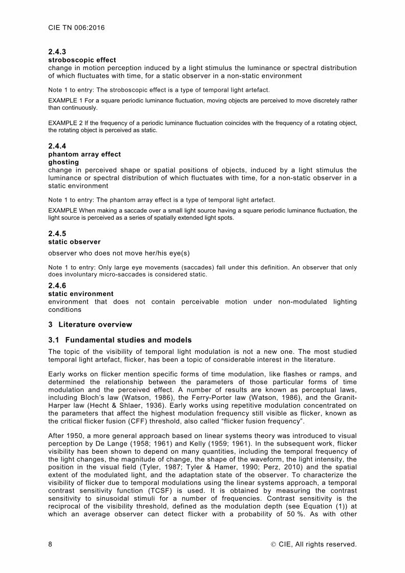
4.3.4 Example embodiments In a particular context, the parameters of the method that were left open in the general frameworks are specified. For the frequency method, these parameters are the sensitivity curve, Tv(f), and the parameter of the Minkowski norm, n. Table 1 gives an overview of an implementation of the method for the visibility quantification of the stroboscopic effect as an example based on the Stroboscopic Effect Visibility Measure introduced by Perz et al. (2014). The sensitivity curve is based on work by Perz et al. (2014) and Wang et al. (2015). It was designed for an application in an office environment, but it can be applied in a broader context. The sensitivity curve in the example was measured in a room with no other light sources except the modulated light source. This results in the most critical situation that can be expected given the context. Note that even though the sensitivity curve is based on data from more than 160 participants, the data come from only two labs and further verification is needed.

————————— 1 Note that the abbreviation of the term “visibility measure”, VM, is often used as quantity symbol, too. This does

not conform with the CIE rules and the rules of other standardizing organizations regarding the presentation of quantity symbols. For that reason the symbol Mv is introduced for the quantity “visibility measure” in this document.

CIE TN 006:2016


Table 1 – Stroboscopic effect visibility measure

Temporal light artefact Stroboscopic effect

Application context General indoor applications, defined by: general illumination, broad spatial distribution; average light level > 100 lx, fully adapted; fastest movements being moderate speed hand

movements <= 4 m/s, movements in the modulated light.

Sensitivity curve /10 Hzv ( )

1( ) 20

1f

a f bT f e

e

,

where f is the frequency in Hz; a = 0,005 18 s; b = 306,6 Hz.

The sensitivity curve is only defined up to 2 000 Hz.

Minkowski norm parameter n = 3,7

Abbreviation SVM

Figure 4 depicts the sensitivity curve defined in Table 1.

Figure 4 – SVM sensitivity curve

In the case of flicker, two sources in literature (Bodington et al., 2015; Perz et al., 2013) recommend the use of n = 2 in the Minkowski norm. These sources, however, apply different sensitivity curves, and further harmonization of the data is needed.

The phantom array effect has not been studied as much as the other two effects. An example shown in Table 2 is derived from the data of Roberts and Wilkins (2013). The sensitivity curve is obtained using a linear interpolation between the two points measured, 10 % at 120 Hz and 100 % at 2 500 Hz. The factor of 4/ in the sensitivity curve is a translation constant from the square waveforms used in the study of Roberts and Wilkins (2013) to sinusoidal waveform used in the general method. Note that the sensitivity curve is based on data from a small number of participants from a single lab.

0

0,2

0,4

0,6

0,8

1

1,2

0 500 1000 1500 2000

Vis

ibili

ty th

resh

old

Frequency / Hz

CIE TN 006:2016


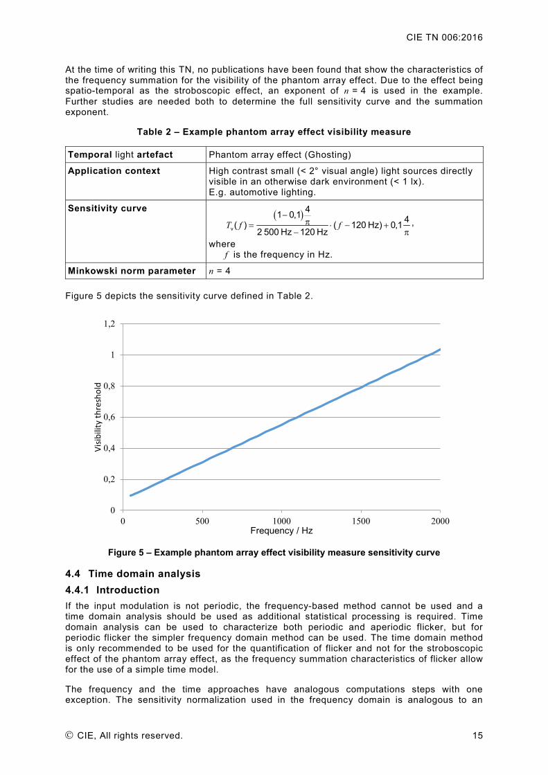
At the time of writing this TN, no publications have been found that show the characteristics of the frequency summation for the visibility of the phantom array effect. Due to the effect being spatio-temporal as the stroboscopic effect, an exponent of n = 4 is used in the example. Further studies are needed both to determine the full sensitivity curve and the summation exponent.

Table 2 – Example phantom array effect visibility measure

Temporal light artefact Phantom array effect (Ghosting)

Application context High contrast small (< 2° visual angle) light sources directly visible in an otherwise dark environment (< 1 lx). E.g. automotive lighting.

Sensitivity curve ( )v

41 0,1 4( ) ( 120 Hz) 0,12 500 Hz 120 Hz

T f f−

π= ⋅ − +− π

,

where f is the frequency in Hz.

Minkowski norm parameter n = 4

Figure 5 depicts the sensitivity curve defined in Table 2.

Figure 5 – Example phantom array effect visibility measure sensitivity curve

4.4 Time domain analysis 4.4.1 Introduction If the input modulation is not periodic, the frequency-based method cannot be used and a time domain analysis should be used as additional statistical processing is required. Time domain analysis can be used to characterize both periodic and aperiodic flicker, but for periodic flicker the simpler frequency domain method can be used. The time domain method is only recommended to be used for the quantification of flicker and not for the stroboscopic effect of the phantom array effect, as the frequency summation characteristics of flicker allow for the use of a simple time model.

The frequency and the time approaches have analogous computations steps with one exception. The sensitivity normalization used in the frequency domain is analogous to an

0

0,2

0,4

0,6

0,8

1

1,2

0 500 1000 1500 2000

Visib

ility

thre

shol

d

Frequency / Hz

CIE TN 006:2016


application of a temporal filter in the time domain. The frequency summation, for a specific Minkowski norm, is analogous to the computation of the short-term variance. Due to the non-periodic nature of the signal, the last step uses statistical processing to quantify the visibility of the temporal light artefact and it is only used in the time domain analysis.

4.4.2 Temporal filtering After the normalization (see 4.3.2), the input modulation is filtered using a context-specific filter to produce an output-filtered waveform. The filter can be implemented either as an analogue filter before sampling or as a digital filter on the sampled waveform. Digital filtering is assumed in this TN. The amplitude response of this filter should correspond to the visibility thresholds for simple sinusoids in the same context, i.e. to the corresponding sensitivity curve (Watson 1986). Some authors (e.g. Hess & Plant, 1985) argue the need for using not one, but two independent temporal filters, corresponding to the two channels in the human visual system each having different time characteristics. In models that use two channels, this step produces two filtered waveforms, one for each channel.

4.4.3 Computing short-term variance and adjustment Next, the filtered waveform is normalized such that the short-term time average is zero. This is done by taking the difference between the waveform and a low-pass filtered version of the waveform. The characteristics of this low-pass filter can be context specific and should be given in the embodiment of the procedure. As a next step, the difference is squared to find the short-term variance of the signal. This step is equivalent to the frequency summation in the case where the Minkowski norm n = 2 is used (equal to the Euclidean norm). Due to possible differences in the duration and sampling frequency, the output of this step needs to be adjusted to ensure proper output. This can be done by using periodic waveforms at prescribed frequencies and modulation depths that result in a just visible temporal light artefact.

4.4.4 Statistical processing The next step is the statistical processing of the short-term variance. In this step, the ordered statistics of the short-term variance are computed, and based on the values of a selected set of ordered statistics the visibility of the temporal light artefacts is quantified. For example, if the value of the 90th percentile is used as a single ordered statistic, then the effect will be visible if there is a probability larger than 10 % of the modulation being more visible than a periodic waveform at visibility threshold.

4.4.5 Example embodiment The IEC Flickermeter (IEC, 2010) is a widely used standard for determining the limits on the allowed voltage modulation. The recent modification of the flickermeter that removes the model of the incandescent bulb can be directly used as a measure for flicker visibility in a general context. The largest problem with the flickermeter is that the temporal filtering used is based on the data of De Lange (1958) for a small visual field and for an observer who is adapted to the flickering frequency. Table 3 gives an overview of an example implementation of the method for the visibility quantification of the short-term flicker severity.

Table 3 – Short-term flicker severity

Temporal light artefact Flicker

Application context General indoor applications, defined by: • direct observation of the light source, small visual

angle ~2°, sharp edge, central vision; • average light level > 100 lx, fully adapted; • adapted to flicker.

Temporal filter and processing

Details of the implementation are described in IEC/TR 61547-1:2015 (IEC, 2015) and in IEC 61000-4-15 (IEC, 2010)

Symbol P st

CIE TN 006:2016


5 Recommendations and future work

TC 1-83 recommends the use of the definitions of temporal light artefacts as given in Clause 2.

In line with the results from the literature overview, the general frameworks given in Clause 4 are recommended to be used for quantification of temporal light artefacts. The frequency-based method according to 4.3 is recommended for the quantification of the visibility of the stroboscopic effect and the phantom array effect. The time-based method according to 4.4 is recommended to quantify flicker. The example embodiments of the general methods given in Clause 4, respectively SVM and the IEC short-term flicker severity, are recommended as methods to quantify the visibility of the stroboscopic effect and flicker, for the appropriate contexts as described in Clause 4.

Future studies are needed to produce additional sensitivity data to validate the measures in the currently defined contexts and extend the applicability of the measures to a wider lighting context.

Further experiments for the quantification of the phantom array effect are needed. Experimental results and theoretical models on the frequency summation are needed as well as more sensitivity data for specific contexts.

For periodic flicker the frequency domain method can be used, and for suitable choices of parameters in the models the same results can be produced by both models. There is, however, no interchangeable implementation of the time domain model in the frequency domain at the moment. For this reason there was no example regarding the frequency domain method for flicker given.

Translating the measures described in this TN into measurement procedures requires detailed analysis of the setup of such a measurement procedure and of the system used. Furthermore, an analysis of the reliability and the reproducibility of both the traditional measures and the new measures and the corresponding frameworks needs to be carried out. For this reason, the formation of a new TC in Division 2 is proposed that will carry out these tasks.

References

ARIAS, M., AITOR, V., JAVIER, S. 2012. An Overview of the AC-DC and DC-DC Converters for LED Lighting Applications. Automatika‒Journal for Control, Measurement, Electronics, Computing and Communications 53 (2), 156-172.

BODINGTON, D., BIERMAN, A., NARENDRAN, N. 2015. A Flicker Perception Metric. Lighting Research and Technology, 1477153515581006.

BULLOUGH, J.D., SWEATER HICKCOX, K., KLEIN, T.R., LOK, A., NARENDRAN, N. 2011. Detection and Acceptability of Stroboscopic Effects from Flicker. Lighting Research and Technology, 44, 477-483.

CAI, R., 2009. Flicker Interaction Studies and Flickermeter Improvement. PhD Research, Eindhoven, Technical University Eindhoven.

CIE 2004. CIE 15:2004 Colorimetry, 3rd Edition. CIE 2011. CIE S 017/E:2011 ILV:International Lighting Vocabulary CIE 2015. CIE S 025/E:2015 Test Method for LED Lamps, LED Luminaires and LED Modules. DE LANGE, H. 1958. Research into the Dynamic Nature of the Human Fovea --> Cortex

Systems with Intermittent and Modulated Light. I. Attenuation Characteristics with White and Colored Light. Journal of the Optical Society of America 48 (11): 777–83.

DE LANGE, H. 1961. Eye’s Response at Flicker Fusion to Square-Wave Modulation of a Test Field Surrounded by a Large Steady Field of Equal Mean Luminance. Journal of the Optical Society of America 51 (4): 415–21.

CIE TN 006:2016


ENGELDRUM, P.G. 2000. Psychometric Scaling: A Toolkit for Imaging Systems Development. Imcotek Press.

FRIER, J.P., HENDERSON, A.J. 1973. Stroboscopic Effect of High Intensity Discharge Lamps. Journal of the Illuminating Engineering Society 3 (1): 83–86.

GARCIA, J., CALLEJA, A.J., LÓPEZ ROMINAS, E., GACIO VAQUERO, D., CAMPA, L. 2011. Interleaved Buck Converter for Fast PWM Dimming of High-Brightness LEDs. Power Electronics, IEEE Transactions on 26 (9): 2627–36.

HECHT, S., SHLAER, S. 1936. Intermittent Stimulation by Light V. The Relation between Intensity and Critical Frequency for Different Parts of the Spectrum. The Journal of General Physiology 19 (6): 965–77.

HESS, R.F., PLANT, G.T. 1985. Temporal Frequency Discrimination in Human Vision: Evidence for an Additional Mechanism in the Low Spatial and High Temporal Frequency Region. Vision Research 25 (10): 1493–1500.

IEC 2010. 61000-4-15:2010 Electromagnetic Compatibility (EMC) - Part 4-15: Testing and Measurement Techniques - Flickermeter - Functional and Design Specifications.

IEC 2013. IEC 61000-3-3:2013 Electromagnetic Compatibility (EMC) - Part 3-3: Limits - Limitation of Voltage Changes, Voltage Fluctuations and Flicker in Public Low-Voltage Supply Systems, for Equipment with Rated Current ≤16 A per Phase and Not Subject to Conditional Connection.

IEC 2015. IEC TR 61547-1:2015 Equipment for General Lighting Purposes - EMC Immunity Requirements - Part 1: An Objective Voltage Fluctuation Immunity Test Method.

IEEE 2015. IEEE Std 1789-2015 IEEE Recommended Practices for Modulating Current in High-Brightness LEDs for Mitigating Health Risks to Viewers.

IESNA 2000. IESNA Lighting Handbook. Edited by Mark Stanley Rea. 9th edition. New York, NY: Illuminating Engineering.

IKEDA, M. 1986. Temporal Impulse Response. Vision Research 26 (9): 1431–40.

IKEDA, M., BOYNTON, R.M. 1965. Negative Flashes, Positive Flashes, and Flicker Examined by Increment Threshold Technique. Journal of the Optical Society of America 55 (5): 560–65.

KELLY, D.H. 1959. Effects of Sharp Edges in a Flickering Field. Journal of the Optical Society of America 49 (7): 730–32.

KELLY, D.H. 1961. Visual Responses to Time-Dependent Stimuli. I. Amplitude Sensitivity Measurements. Journal of the Optical Society of America 51 (4): 422–29.

KELLY, D.H. 1971. Theory of Flicker and Transient Responses, I. Uniform Fields. Journal of the Optical Society of America 61 (4): 537–46.

LEVINSON, J. 1960. Fusion of Complex Flicker II. Science 131 (3411): 1438–40. MULLIGAN, M.D., BROACH, B., LEE, T.H. 2007. A 3MHz Low-Voltage Buck Converter with

Improved Light Load Efficiency. In 2007 IEEE International Solid-State Circuits Conference. Digest of Technical Papers, 528–620.

REA, M.S., OUELLETTE, M.J. 1988. Table-Tennis under High Intensity Discharge (HID) Lighting. Journal of the Illuminating Engineering Society 17(1). 29-35.

PERZ, M. 2010. Flicker Perception in the Periphery. Master thesis, Eindhoven, Technical University Eindhoven.

PERZ, M., VOGELS, I.M.L.C., SEKULOVSKI, D., WANG, L., TU, Y., HEYNDERICKX, I.E.J. 2014. Modeling the Visibility of the Stroboscopic Effect Occurring in Temporally Modulated Light Systems. Lighting Research and Technology, May, 1477153514534945.

PERZ, M., VOGELS, I.M., SEKULOVSKI, D. 2013. Evaluating the Visibility of Temporal Light Artifacts. In Proceedings of Lux Europa 2013 – the 12th European Lighting Conference. Krakow.

CIE TN 006:2016


POPLAWSKI, M.E., MILLER, N.M. 2013. Flicker in Solid-State Lighting: Measurement Techniques, and Proposed Reporting and Application Criteria. In Proceedings of CIE Centenary Conference “Towards a New Century of Light“. Paris.

POUSSET, N., ROUGIÉ, B., RAZET, A. 2010. Impact of Current Supply on LED Colour. Lighting Research and Technology 42 (4): 371–83.

RASHBASS, C. 1970. The Visibility of Transient Changes of Luminance. The Journal of Physiology 210 (1): 165–86.

ROBERTS, J.E., WILKINS, A.J. 2013. Flicker Can Be Perceived during Saccades at Frequencies in Excess of 1 kHz. Lighting Research and Technology 45 (1): 124–32.

ROUFS, J.A.J. 1972. Dynamic Properties of vision—I. Experimental Relationships between Flicker and Flash Thresholds. Vision Research 12 (2): 261–78.

ROUFS, J.A.J., BLOMMAERT, F.J.J. 1981. Temporal Impulse and Step Responses of the Human Eye Obtained Psychophysically by Means of a Drift-Correcting Perturbation Technique. Vision Research 21 (8): 1203–21.

SCHUBERT, E. F., KIM, J. K. 2005. Solid-State Light Sources Getting Smart. Science 308 (5726): 1274–78.

SCHUBERT, E.F., KIM, J.K., LUO, H., Xi, J.Q. 2006. Solid-State Lighting—a Benevolent Technology. Reports on Progress in Physics 69 (12): 3069.

SEKULOVSKI, D., VOGELS, I., CLOUT, R., PERZ, M. 2011. Changing Color over Time. In Ergonomics and Health Aspects of Work with Computers, edited by Michelle M. Robertson, 218–25. Springer Berlin Heidelberg.

SHADY, S., MACLEOD, D.I.A., FISHER, H.S. 2004. Adaptation from Invisible Flicker. Proceedings of the National Academy of Sciences of the United States of America 101 (14): 5170–73.

SHEPARD, R.N. 1987. Toward a Universal Law of Generalization for Psychological Science. Science 237 (4820): 1317–23.

STORK, D.G., FALK, D.S. 1987. Temporal Impulse Responses from Flicker Sensitivities. JOSA A 4 (6): 1130–35.

SWANSON, W.H., UENO,T., SMITH, V.C., POKORNY, J. 1987. Temporal Modulation Sensitivity and Pulse-Detection Thresholds for Chromatic and Luminance Perturbations. JOSA A 4 (10): 1992–2005.

TYLER, C.W. 1992. Psychophysical Derivation of the Impulse Response through Generation of Ultrabrief Responses: Complex Inverse Estimation without Minimum-Phase Assumptions. JOSA A 9 (7): 1025–40.

TYLER, C.W. 1987. Analysis of visual modulation sensitivity. III: Meridional variation in peripheral flicker sensitivity. JOSA A 4 (8): 1612.

TYLER, C.W, HAMER, R.D. 1990. Analysis of Visual Modulation Sensitivity. IV. Validity of the Ferry–Porter Law. JOSA A 7 (4): 743–58.

VOGELS, I.M.L.C., SEKULOVSKI, D., PERZ, M. 2011. Visible Artefacts of LEDs. In 27th Session of the CIE. Sun City, South Africa: CIE.

WANG, L., TU, Y., LU, L., PERZ, M., VOGELS, I.M.L.C., HEYNDERICKX I.E.J. 2015. 50.2: Invited Paper: Stroboscopic Effect of LED Lighting. In SID Symposium Digest of Technical Papers 46:754–57. Wiley Online Library.

WATSON, A.B. 1982. Derivation of the Impulse Response: Comments on the Method of Roufs and Blommaert. Vision Research 22 (10): 1335–37.

WATSON, A.B. 1986. Temporal Sensitivity. In Handbook of Perception and Human Performance, edited by K. Boff, L. Kaufman, and J. Thomas. New York: Wiley.

WILKINS, A., VEITCH, J., LEHMAN, B. 2010. LED Lighting Flicker and Potential Health Concerns: IEEE Standard PAR1789 Update. In 2010 IEEE Energy Conversion Congress and Exposition (ECCE), 171–78.

CIE TN 006:2016files.cie.co.at/883_CIE_TN_006-2016.pdf · TECHNICAL NOTE . Visual Aspects of...

Documents

Transcript of CIE TN 006:2016files.cie.co.at/883_CIE_TN_006-2016.pdf · TECHNICAL NOTE . Visual Aspects of...