Pattern of Trade and EconomicDevelopment in the Model

of Monopolistic Competition

Jeffrey D. Sachs, Xiaokai Yang,and Dingsheng Zhang

CID Working Paper No. 14April 1999

© Copyright 1999 Jeffrey D. Sachs, Xiaokai Yang, Dingsheng Zhang,and the President and Fellows of Harvard College

Working PapersCenter for International Developmentat Harvard University

CID Working Paper no. 14

Pattern of Trade and Economic Developmentin the Model of Monopolistic Competition

Jeffrey D. Sachs, Xiaokai Yang, and Dingsheng Zhang

Abstract

The paper introduces differences in production and transaction conditions between countries into

the model of monopolistic competition to investigate the interplay between trade policies and

development strategies. It applies inframarginal analysis, which is total benefit analysis between

corner solutions in addition to marginal analysis of each corner solution, to show that as

transaction conditions are improved, the general equilibrium may discontinuously jump across

different patterns of trade and economic development. It compares the marginal and

inframarginal comparative statics of equilibrium in the model of monopolistic competition with

the core theorems in the neoclassical trade models and with conventional wisdom in

development economics. It shows that as analytical framework is altered, the meanings of

concepts and related empirical observations will be changed too.

Keywords: trade pattern, development strategy, income distribution, terms of trade

JEL codes: F12, F13, O10

Jeffrey D. Sachs is the Director of the Center for International Development and the HarvardInstitute for International Development, and the Galen L. Stone Professor of International Tradein the Department of Economics. His current research interests include emerging markets,global competitiveness, economic growth and development, transition to a market economy,international financial markets, international macroeconomic policy coordination andmacroeconomic policies in developing and developed countries.

Xiaokai Yang is a Research Fellow at the Center for International Development. His researchinterests include equilibrium network of division of labor, endogenous comparative advantages,inframarginal analysis of patterns of trade and economic development.

Dingsheng Zhang is Professor of Research Center of Economics, Wuhan University. His currentresearch interests include dual structure in economic development, economic development andincome distribution, equilibrium models of monopolistic competition, trade pattern anddevelopment strategies.

CID Working Paper no. 14

Pattern of Trade and Economic Developmentin the Model of Monopolistic Competition

Jeffrey D. Sachs, Xiaokai Yang, and Dingsheng Zhang

1. Introduction

The purpose of this paper is twofold. First we investigate trade pattern in a general equilibrium

model of monopolistic competition with transaction costs in comparison with the four core

theorems, the Heckscher-Olin (HO) theorem, the Stolper-Samuelson (SS) theorem, the

Rybczynski (RY) theorem, and factor price equalization (FPE) theorem in the HO model.

Second, we introduce differences in transaction conditions between countries into the model of

monopolistic competition to investigate interplay between trade patterns and development

strategies. Let us motivate the two tasks one by one.

According to Trefler (1995), the HO theorem is consistent with empirical findings only

50% of the time. Grossman and Levinsohn (1989) show that the specific factor model captures

reality more closely than the SS theorem for many U.S. industries.1

There are several lines of research that might accommodate the new empirical evidences.

Leontief (1953) suggested to introduce technological differences between countries into the HO

model to accommodate observations. Trefler (1995) demonstrated empirically that a

modification is desirable that allows for consumption bias and technology difference between

countries. Bhagwati and Dehejia (1994, pp.39, 42) indicate that the assumptions of the SS and

FPE theorems remain so extraordinarily demanding that they cannot be taken seriously as the

major theoretical construct justifying fears in industrial countries that trade with developing

countries will undermine the wages of unskilled labor. They note that considerable analytical

work was devoted to showing why FPE seemed to be frustrated in reality. They suggest three

ways to invalidate the SS theorem and FPE theorem. One is to consider the equilibrium that

occurs outside of the diversification cone and discontinuous jumps of equilibrium between

different patterns of specialization. Another is to consider the CES production function. In the

face of a sufficiently large shift in relative factor prices, goods could switch over from being

intensive in one factor to being intensive in the other (factor reversal). Finally, scale economies

could be another reason for de facto differences in technology and, in particular, could invalidate

2

the SS theorem, causing both factors real wages to rise (p. 44) as scale efficiencies from trade

swamp adverse effects on the scarce factor.

Cheng, Sachs, and Yang (1998) introduce differences in technology and in transaction

conditions between the countries into the HO model and conduct inframarginal analysis of jumps

of equilibrium between various patterns of specialization to confirm these suggestions.

Panagariya (1983), Kemp (1991), Young (1991), and others introduce variable returns to scale to

refine the core theorems. Helpman and Krugman (1985) explore effects of economies of scale

and monopolistic competition on trade pattern. For instance, Helpman (1987) shows that when

economies become more similar in size, world trade increases. However, because of symmetry in

their models, it is indeterminate which country exports which goods in equilibrium.

In the Ricardo model of exogenous comparative advantage (see Dixit and Norman,

1980), trade pattern is explained by exogenous comparative advantage in technologies. Here,

exogenous comparative advantages come from ex ante differences between agents before they

have made decisions. In the literature of endogenous specialization (see Yang and Ng, 1998 for a

recent survey of this literature and references there), trade pattern is explained by endogenous

comparative advantage. Endogenous comparative advantage comes from increasing returns. It

may exist between ex ante identical agents. Individuals trade those goods which have greater

economies of specialization, better transaction condition, and/or are more desirable if not all

goods are traded (see Yang, 1991). But who sells which good is indeterminate in the models of

endogenous specialization because of the assumption that all individuals are ex ante identical.

The current paper shall investigate the implications of coexistence of endogenous and exogenous

comparative advantage and transaction costs for economic development and trade.

Puga and Venables (1998) introduce difference in endowment between countries into the

model of monopolistic competition. But as they come to comparative statics of equilibrium, the

difference is assumed away. In the current paper, we introduce difference in transaction and

production conditions between countries into the model of monopolistic competition to

investigate pattern of trade in the model of monopolistic competition in comparison with

neoclassical core trade theorems in the HO model. Our purpose is not only checking under what

conditions the core theorems hold (or do not hold), but also investigating effects of changes in

framework on changes of the meanings of the concepts, such as factor intensity and gains from

trade. As the meanings of the concepts change in response to changes in model structure,

3

relevance of empirical evidence that is obtained on the basis of the neoclassical framework to the

framework of monopolistic competition may be in question.

As Albert Einstein stated (quoted in Heisenberg, 1971, p. 31), "It is quite wrong to try

founding a theory on observable magnitudes alone. … It is the theory which decides what we can

observe." For instance, many economists take the notion of capital as granted. But its meaning in

the model of endogenous number of intermediate (capital) goods is totally different from that in

a neoclassical HO model. As the number of capital goods that are employed to produce a final

good increases in response to improvements in transaction conditions, the equilibrium input level

of capital and capital intensity increase even if production conditions, tastes, and equilibrium

prices are not changed. Hence, in a model of monopolistic competition, outsourcing,

disintegration, and variety of goods might be better concepts than the notion of capital to capture

the essence of comparative statics of equilibrium. Hence, data sets that are designed according to

the new concepts might be more appropriate for testing the new theory.

Many new models of monopolistic competition with transaction costs are used to analyze

trade and development phenomena. For instance Krugman and Venables (1995) analyze

industrialization and income distribution, Fujita and Krugman (1995) analyze urbanization by

introducing difference of transaction conditions between industrial and agricultural sectors into

the model of monopolistic competition. Puga and Venables (1998) analyze import substitution

and geographical concentration of industrial production. As the essence of comparative statics of

equilibrium in this kind of models is increasingly more appreciated, we can see that many

conventional notions, such as import substitution, become out-of-date. Rethinking of the

relationship between trade pattern and economic development pattern is needed.1

Hence, the second purpose of the current paper is to investigate the interplay between

trade pattern and development pattern in a model of monopolistic competition. Feenstra (1998)

reviews empirical evidences for the relationship between increases in trade of intermediate inputs

and economic development. He points out that the distinction between effects of trade and

effects of technological changes on income distribution becomes suspect if we consider

1 Another example of interdependence between notions and framework that are used relates to the concepts ofskilled versus unskilled workers. In a model of endogenous variety of intermediate goods, this distinction can bereplaced with difference in the number of professional sectors. An increase in variety of occupations implies thatmore professional workers are available, which is equivalent to an increase of skilled workers. Allyn Young (1928)called this variety of professional occupations "qualitative aspect of division of labor." He referred to economies ofscale as "quantitative aspect of division of labor."

4

equilibrium comparative statics in a model of endogenous number of intermediate goods. As

transaction conditions are improved (due to new communication and transacting technology) the

number of intermediate goods increases, final goods become more "capital intensive," and

outsourcing trade increases. Our general equilibrium comparative statics in the framework of

monopolistic competition will assist clarifying the discussion in which vague logic and

inaccurate terms are sometimes used.

As we introduce exogenous comparative advantage in production (based on ex ante

differences in production conditions between countries) and exogenous comparative advantage

in transactions (based on ex ante differences in transaction conditions between countries) into the

model with monopolistic competition and endogenous comparative advantage (based on

economies of scale), we can show that a country may export goods in which it has exogenous

comparative disadvantage in production if its endogenous comparative advantages in production

and exogenous comparative advantage in transactions outweigh its exogenous comparative

disadvantage. Also, final manufactured goods may become increasingly more capital intensive,

as the number of capital goods increases in response to parameter changes. A country can export

capital intensive goods even if it has exogenous comparative disadvantage in producing this

good.

Our model will show that a country will trade goods in which it has net comprehensive

exogenous and endogenous comparative advantage in production as well as in transactions. It

will exploit substitution between trades of different types of goods to avoid trade that involves

high transaction costs. Various possible substitutions between endogenous and exogenous

comparative advantages and between comparative advantages in production and in transactions

generate much more colorful picture of equilibrium trade and development patterns than in

neoclassical trade models.

Section 2 specifies the model, identifies possible trade patterns, and solves for local

equilibrium in each trade pattern. Section 3 conducts inframarginal analysis across different trade

patterns and identifies parameter subspaces within each of which a local equilibrium is the

general equilibrium. In section 4, our results are compared with conventional wisdom in

neoclassical theories of trade and economic development. Final section concludes the paper.

5

2. The Model and Local Equilibria and Marginal Comparative Statics in Various Trade

Structures

Consider two countries. Population size in country i is Mi. Migration between countries is

prohibitively expensive. Agricultural good z is produced from labor. Industrial good y is

produced from labor and n intermediate goods.

2.1. A consumer's decision

A representative consumer's decision problem in country i is

(1) Max: ui = (yi + kiyji)α (zi +kizji)

1-α s.t. piy yi+ pjyyji + pizzi + pjzzji

= wi

where ui is a consumer's utility level in country i, yi and zi are the respective quantities of the

manufactured consumption good (such as car) and the agricultural good (such as food), purchased

from the domestic market in country i. yji and zji

are the respective quantities of the two goods

imported by an individual in country i from the other country. pis is the price of good s in country i.

It is assumed that each individual is endowed with one unit labor, and labor in country 1 is the

numeraire, so that w1 = 1 and w2 = w. Iceberg transaction cost is assumed, so that 1-ki ∈ [0, 1] is

the transaction cost coefficient and ki the transaction efficiency coefficient for importing one unit

of final consumption goods in country i.

2.2. Possible Trade Structures

As we introduce the ex ante differences in transaction conditions between the two countries into

the model, corner solutions are possible. Hence, standard marginal analysis for interior solutions

does not work. We need a little bit of innovation of analytical method. We first apply the Kuhn-

Tucker condition to identify the conditions under which a particular trade structure occurs in

equilibrium. These conditions are dependent on relative prices. Second, for a given structure, we

solve for a local equilibrium using marginal analysis. We can plug the equilibrium prices into the

conditions identified in the first step. We can then partition parameter space into subspaces

within each of which a particular structure occurs in equilibrium. This is called inframarginal

analysis.

Let us take the first step in the inframarginal analysis. The Kuhn-Tucker condition for the

two representative consumers' decision problems in the two countries indicates that some trade

6

structures never occur in equilibrium and that each of the feasible trade structures occurs in

equilibrium only if relative prices and relative transaction condition in the two countries satisfy a

certain condition. Later, we can obtain similar result for trade pattern of intermediate goods using

the Kuhn-Tucker condition for the decision of a firm producing the final manufactured good.

The two sets of the Kuhn-Tucker conditions yield the following conditions for a certain trade

pattern to occur in equilibrium, where xi is the amount of an intermediate good purchased from

the domestic market in country i, xji is the amount of an intermediate good imported from country

j to country i, and ti is the transaction efficiency coefficient of importing intermediate goods in

country i.

(2)

(A) If k1 and t1 and/or k2 and t2 are sufficiently small, the optimum decision requires that zji = xji =

yji = 0 and xi, yi, zi >0, which implies that no trade occurs between the countries or autarky

structure, shown in Fig. 1(a), occurs in equilibrium.

(C1) For p1y/p2y <k2 and p1z/p2z >1/k1, the optimum decision requires z12 = x12 = y21 = z1 = y2 = 0

and x1, y1, z2, x21, z21, y12 >0. This structure of trade (C1) is shown in Fig. 1(c).

(C2) For p1y/p2y > 1/k1 and p1z/p2z < k2, the optimum decision requires z21 = x21 = y12 = z2 = y1 = 0

and x2, y2, z1, x12, z12, y21>0. This structure of trade C2 is symmetric to C1.

(D0) For p1y/p2y ∈(k2, 1/k1) and p1z/p2z ∈(k2, 1/k1), the optimum decision requires z12 = y12 = z21 =

y21 = 0 and x1, y1, z1, x2, y2, z2, x12, x21 > 0. This structure of trade (D0) is shown in Fig. 1(d).

(D1) For p1y/p2y ∈(k2, 1/k1) and p1z/p2z < k2, the optimum decision requires y12 = z21 = y21 = z2 = 0

and x1, y1, z1, x2, y2, x12, x21, z12 > 0. This structure of trade is called D1.

(D2) For p1y/p2y ∈(k2, 1/k1) and p1z/p2z > 1/k1, the optimum decision requires y21 = z12 = y12 = z1 =

0 and x2, y2, z2, x1, y1, x21, x12, z21 > 0. This structure of trade D2 is symmetric to D1.

(E1) For p1y/p2y <k2 and p1z/p2z ∈(k2, 1/k1), the optimum decision requires x12 = z12 = y21 = z21 = x2

= y2 = 0 and x1, y1, z1, x21, y12, z2 > 0..This trade structure is called E1, shown in panel (e).

(E2) For p1y/p2y > 1/k1 and p1z/p2z ∈(k2, 1/k1), the optimum decision requires x21 = z21 = y12 = z12 =

x1 = y1 = 0 and x2, y2, z2, x12, y21, z1 > 0. This trade structure E2 is symmetric to E1.

(F1) For p1y/p2y <k2 and p1z/p2z < k2, the optimum decision requires x12 = y21 = z21 = x2 = z2 = y2 = 0

and x1, y1, z1, x21, y12, z12 > 0. This trade structure is called F1, shown in panel (f).

7

(F2) For p1y/p2y > 1/k1 and p1z/p2z > 1/k1, the optimum decision requires x21 = y12 = z12 = x1 = z1 =

y1 = 0 and x2, y2, z2, x12, y21, z21 > 0. This trade structure is called F2.

(a) Structure A (autarky) (b) A structure that does not occur in equilibrium

(c) Structure C1 (d) Structure D0

(e) Structure E1 (f) Structure F1

Figure 1: Different Patterns of Development and Trade

Also, it can be shown that a pattern of trade in panel (b) and other trade structures do not occur in

equilibrium except for some razor edge cases where some of the inequalities involving relative

prices in (2) become equalities.2 The markets for goods y and z are competitive because of

constant returns to scale in production. But the market for intermediate goods is monopolistically

competitive.

2 The complete partition of the parameter space when the razor edge cases are considered can be obtained from theauthors upon request.

8

2.3. Production of agricultural good z

The production function of food in country i is

Zi = θiLiz

where Zi is the output level of z, and Liz is the amount of labor allocated to the production of food

in country i. For simplicity, we assume that θ2 =1 and θ1 = θ > 1. This implies that country 1 has

exogenous comparative advantage in producing food, since in the next two subsections the

production function of industrial goods y and x is assumed same for the two countries.

2.4. Production of final manufactured good y

The production function for a representative car manufacturer's production function in country i is

Yi = [nixiρ +(n-ni)(tixji)

ρ]β/ρLiy1-β

where Yi is output level of good y produced by a representative firm in country i, ni and n-ni are the

respective numbers of intermediate goods purchased by country i from domestic market and from

the other country, xi is the amount of an intermediate good purchased by the firm in country i from

domestic market to produce good y, xji is that purchased by the firm in country i from the other

country, and ti is the transaction efficiency coefficient for country i importing intermediate good

from the other country. x can be considered as all kinds of professional machine tools, and the

elasticity of substitution 1/(1-ρ) is assumed to be larger than one, that is ρ∈(0,1). We have used the

symmetry and omit index of intermediate goods when no confusion is caused.

2.5. Production of intermediate goods

The production function for the monopolist producer of an intermediate good in country i is

Xi = (Li-a)/b,

where Xi is the quantity of an intermediate good supplied by the monopolist in country i and Li is

the amount of labor hired by the firm to produce the intermediate good. Again, we have used the

symmetry and omit index of intermediate goods when no confusion is caused.

As shown in (2), ten market structures may occur in equilibrium in this model. We consider

the local equilibrium in each of them.

9

2.6. Local equilibrium in structure A

We first consider structure A where xi, yi, zi > 0, xij = yij = zij = 0. A consumer's decision yields

demand functions for goods y and z. Each consumer supplies one unit of labor and total supply of

labor in country i is Mi. The zero profit condition for the firm producing z gives the price of good z

in terms of labor in country i piz, The symmetry implies that quantities supplied or employed are

the same for ni intermediate goods. The zero profit condition and a first order condition for the

decision problem of the firm producing y yields the equilibrium relative quantity of labor and

intermediate goods and an equation that determines the equilibrium piy/pix. Using the production

and demand functions of y, the market clearing conditions for y and labor, and the first order

conditions for the decision problem of the firm producing y, we can find the demand function for

x. Using the Dixit-Stiglitz formula for own price elasticity E = 1/(1-ρ), we can then work out the

first order condition for the decision problem for the monopolist producer of an intermediate good.

Then the zero profit condition for this firm yields the equilibrium ni. The local equilibrium and its

marginal comparative statics in this structure is summarized as follows.

wi = 1, p1z = 1/θ, p2z = 1, pix =b/ρ,

piy = (1-β)β-1[a/(1-ρ)β]β/ρ [(1-ρ)b/ρa]β (αMi)β (1-1/ρ),

ni = Miβα(1-ρ)/a,

u1 = [θ(1-α)](1-α)ααp1y-α, u2 = (1-α)(1-α)ααp2y

-α,

dpiy/dMi < 0, dni/dMi > 0, dui/dMi > 0.

where i = 1, 2. The marginal comparative statics imply that as the population in an integrated

market increases, the equilibrium price of final manufactured good decreases and the equilibrium

number of intermediate goods and per capita real income increase. Since total factor productivity

of the final manufactured good is an increasing function of the number of intermediate goods, this

productivity increases with population size too. Ethier (1980) uses this result to show that the

opening up of international trade can increase the population size in an integrated world market.

This enlarges the scope for trading off economies of scale against productivity gains from more

variety of intermediate goods and therefore generates gains from trade.

2.7. Local equilibrium in structure C

Next, we consider structure C1 where x1, y1, z2, y12, x21 > 0, x12 = y21 = z12 = 0. The procedure to

solve the corner equilibrium in this structure is the same as that for structure A except that the

10

markets for x, y, z are jointly cleared for both countries. The corner equilibrium in this structure is

summarized as follows.

w = t1ρ, p1z = 1/θ, p2z = t1

ρ, p1x =b/ρ, p2x = t1ρb/ρ,

p1y = (1-β)β-1β-β/ρ (b/ρ)β [(1-ρ)α(M1+ k1ρM2)/a] β (1-1/ρ),

n1 = [(1-ρ)/a][M1(βα+1-α)-α(1-β)t1ρM2],

n2 = [(1-ρ)/a][M2α-(1-α)t1-ρM1],

u1 = B(θk1)1-αt1

-ρ(1-α)(M1+t1ρM2)

αβ(1-ρ)/ρ, u2 = Bt1ραk2

α(M1+t1ρM2)

αβ(1-ρ)/ρ,

where B ≡ (1-α)(1-α)αα [(1-β)1-βββ/ρ(ρ/b)β]α[α(1-ρ)/a]αβ(1-ρ)/ρ. The differentiation of the solutions

yields marginal comparative statics of the local equilibrium in structure C1.

(3) dni/dMi > 0, dni/dMj < 0, dn2/dt1 > 0, dn1/dt1 < 0,

dn/dt1 > 0, if (1-α)M1/α(1-β)M2 > t12ρ,

dn/dM1 > 0 iff t1>[(1-α)/αβ+1-α]1/ρ, dn/dM2 > 0,

dw/dt1 > 0, dui/dMj > 0, dui/dki > 0, dui/dt1 > 0.

where i, j = 1, 2 and n = n1 + n2 is the number of all intermediate goods available in the two

countries. The marginal comparative statics of the local equilibrium imply that as the transaction

condition in country 1 improves, the production of intermediate goods will shift from country 1 to

country 2. This relocation of industrial production increase utility levels in the two countries

although the nominal income in country 1 relative to that in country 2 increases as well. The

improvement of the transaction condition in country 2 has no effects on industrial structure and

location of industrial production, though it increases utility of each individual in country 2. An

increase in the population size in country 1 will shift the production of producer goods from

country 2 to country 1. But an increase in the population size in country 2 has opposite effect on

location of industrial production. However, the increase in population size in either country will

raise per capita real income in both countries.

As n1 or n2 tends to zero, the production of all intermediate goods becomes concentrated in

country 2 or 1. A careful examination of the equilibrium solutions yields the following conditions

for such concentration.

(4) n1 = n and n2 = 0 if t1 < ta ≡ [M1(1-α)/M2α]1/ρ

n1, n2 ∈ (0, n) if t1 ∈ (ta, tb), where tb ≡ [M1(αβ+1-α)/M2α(1-ρ)]1/ρ

n2 = n and n1 = 0 if t1 > tb,

11

where ta< tb always holds. The marginal comparative statics of the local equilibrium in structure C1

are summarized in the following proposition.

Proposition 1:

If the transaction efficiency of intermediate goods is very low in country 1, country 2 specializes in

producing the agricultural good in the absence of industrialization. The production of all final and

intermediate manufactured goods is located in country 1. As the transaction condition is improved

in country 1, country 2 starts industrialization which relocates the production of intermediate goods

from country 1 to country 2. The smaller the population size of country 1 relative to country 2, the

faster is the relocation process. Per capita real incomes in both countries increase as a result of the

relocation, although wage rate in country 2 increases compared to that in country 1. The wage

difference between the two countries converges to 0 as transaction cost tends to 0. The per capita

real income in country 1 is more likely to be higher than in country 2, the greater the income share

of the final manufactured good, the greater the elasticity of substitution between intermediate

goods, and/or the higher the relative transaction efficiency of country 1 to country 2. An increase in

the population size of a country will move the production of intermediate goods to this country

from the other country, increasing per capita real income in this country.

The local equilibrium in structure C2 is symmetric to that in C1. Hence, a similar proposition can

be obtained from the comparative statics of that local equilibrium.

2.8. Local equilibrium in structure D

We now consider structure D0 in which country 1 produces final goods y and z and n1 intermediate

goods. It exchanges the intermediate goods for n2 intermediate goods produced by country 2 which

self-provides goods y and z as well. Hence, for this structure we have xi, yi, zi, xij > 0, yij = zij = 0.

The local equilibrium in this structure is summarized as follows.

w is given by f = M1 + t1ρ/(1-ρ) [M2w

-ρ/(1-ρ)-M1w-1/(1-ρ)-M2w

-(1+ρ)/(1-ρ) t2-ρ/(1-ρ)] = 0

p1z = 1/θ, p2z = 1, p1x =b/ρ, p2x = wb/ρ,

p1y = A(M1/t1)β [(t1

ρ/(ρ-1)-t2ρ/(1-ρ))/(1-t2

ρ/(1-ρ)w1/(1-ρ))]β [M1t11/(ρ-1)+M2w

ρ/(ρ-1)]-β/ρ

p2y = wAM2β[(t1

ρ/(ρ-1)-t2ρ/(1-ρ))/(t1

ρ/(ρ-1)w1/(1-ρ)-1)]β [M1t21/(1-ρ)+M2w

ρ/(ρ-1)]-β/ρ

ni = β(1-ρ)Mi/a,

12

u1 = [θ(1-α)]1-αααp1y-α, u2 = (1-α)1-ααα (p2y/w)-α.

where A ≡ (1-β)β-1αβ[a/(1-ρ)β]β/ρ[(1-ρ)b/aρ]β. The market clearing conditions for intermediate

goods and the first order conditions for producers of good y in the two countries require

w∈(t1ρ, t2

-ρ).

where t1ρ< t2

-ρ always holds. It is obvious that w converges to 1 as t1 and t2 tend to 1.

The differentiation of the solutions yields:

dw/dt1 = -(∂f/∂ t1)/(∂f/∂w) > 0, dw/dt2 = -(∂f/∂ t2)/(∂f/∂w) < 0,

where ∂f/∂t1 > 0, ∂f/∂t2 < 0, ∂f/∂w < 0. The result implies that relative per capital nominal income

of country 2 to country 1 increases as the transaction condition in country 1 improves or as the

transaction condition in country 2 worsens.

Similar results can be obtained for the relationship between per capita real income in a

country and the transaction conditions in the two countries. It can be shown that

(5a) du1/dt1 = (∂u1/∂t1)+(∂u1/∂w)(dw/dt1) < 0,

du2/dt2 = (∂u2/∂t2)+(∂u2/∂w)(dw/dt2) < 0,

where dw/dt1 > 0, dw/dt2 < 0, ∂u1/∂w < 0, ∂u2/∂w > 0, ∂u1/∂ t1 < 0, ∂u1/∂t2 < 0, ∂u2/∂t2 < 0.

Other marginal comparative statics in this structure are

(5b) dui/dMi > 0, dui/dMj > 0, dni/dMi > 0, dni/dρ < 0, dni/da < 0.

The Kuhn-Tucker condition for a producer of good y indicates that the first order derivative

of profit with respect to quantity of an imported intermediate good is always negative if the

transaction efficiency coefficient is zero in this country. Hence, the equilibrium will jump to

another structure if t is sufficiently close to 0 in either country.

If 1-ti is interpreted as the import tariff rate in country i and all tariff revenue is exhausted

by bureaucrats who collect it, then the marginal comparative statics in (5) imply that each country

has an incentive to impose tariff which increases per capita real income in the home country.

Proposition 2:

As the population size in either country or import tariff rate increases in a country, the per capita

real income in this country increases. Also, the number of intermediate goods produced in a

country increases with its population size. Wage difference between the two countries converges to

0 as transaction cost tends to 0.

13

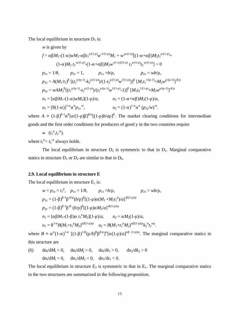
The local equilibrium in structure D1 is:

w is given by

f = αβM1-(1-α)wM2-αβt1ρ/(1-ρ)w-1/(1-ρ)M1 + w-ρ/(1-ρ)[(1-α+αβ)M2t1

ρ/(1-ρ)+

(1-α)M2 t2-ρ/(1-ρ)-(1-α+αβ)M2w

-(1+ρ)/(1-ρ) t1ρ/(1-ρ)t2

-ρ/(1-ρ)] = 0

p1z = 1/θ, p2z = 1, p1x =b/ρ, p2x = wb/ρ,

p1y = A(M1/t1)β [(t1

ρ/(ρ-1)-k2ρ/(1-ρ))/(1-t2

ρ/(1-ρ)w1/(1-ρ))]β [M1t11/(ρ-1)+M2w

ρ/(ρ-1)]-β/ρ

p2y = wAM2β[(t1

ρ/(ρ-1)-t2ρ/(1-ρ))/(t1

ρ/(ρ-1)w1/(1-ρ)-1)]β [M1t21/(1-ρ)+M2w

ρ/(ρ-1)]-β/ρ

n1 = [αβM1-(1-α)wM2](1-ρ)/a, n2 = (1-α+αβ)M2(1-ρ)/a,

u1 = [θ(1-α)]1-αααp1y-α, u2 = (1-α)1-ααα (p2y/w)-α.

where A ≡ (1-β)β-1αβ[a/(1-ρ)β]β/ρ[(1-ρ)b/aρ]β. The market clearing conditions for intermediate

goods and the first order conditions for producers of good y in the two countries require

w∈(t1ρ,t2

-ρ).

where t1ρ< t2

-ρ always holds.

The local equilibrium in structure D2 is symmetric to that in D1. Marginal comparative

statics in structure D1 or D2 are similar to that in D0.

2.9. Local equilibrium in structure E

The local equilibrium in structure E1 is:

w = p2z = t1ρ, p1z = 1/θ, p1x =b/ρ, p2x = wb/ρ,

p1y = (1-β)β-1β-β/ρ(b/ρ)β[(1-ρ)α(M1 +M2t1ρ)/a]-β(1-ρ)/ρ

p2y = (1-β)β-1β-β (b/ρ)β[(1-ρ)αM2/a]-β(1-ρ)/ρ

n1 = [αβM1-(1-β)α t1ρM2](1-ρ)/a, n2 = αM2(1-ρ)/a,

u1 = θ1-αB(M1+t1ρM2)

αβ(1-ρ)/ρ u2 = B(M1+t1ρM2)

αβ(1-ρ)/ρk2αt1

αρ.

where B ≡ αα(1-α)1-α [(1-β)1-β(ρ/b)βββ/ρ]α[α(1-ρ)/a]αβ (1-ρ)/ρ. The marginal comparative statics in

this structure are

(6) dui/dMi > 0, dui/dMj > 0, dui/dt1 > 0, du2/dk2 > 0

dni/dMi > 0, dn1/dM2 < 0, dn1/dt1 < 0.

The local equilibrium in structure E2 is symmetric to that in E1. The marginal comparative statics

in the two structures are summarized in the following proposition.

14

Proposition 3:

As transaction efficiency and population size increases in either country, per capita real incomes in

both countries increase. The number of intermediate goods produced in a country increases with

the population size in this country. The number of intermediate goods produced by the country

importing intermediate goods decreases with the population size in the other country and with the

transaction efficiency coefficient in this country.

2.10. Local equilibrium in structure F

The local equilibrium in structure F1 and its marginal comparative statics are:

(7) w = p2z = t1ρ, p1z = 1/θ, p1x =b/ρ, p2x = wb/ρ,

p1y = (1-β)β-1(b/ρ)ββ-β/ρ[(1-ρ)α(M1+t1ρM2)/a]

p2y = (1-β)β-1β-β (b/ρ)β[(1-ρ)M2/a]-β(1-ρ)/ρ

n1 = [αβM1-(1-αβ)t1ρM2](1-ρ)/a, n2 = M2(1-ρ)/a,

u1 = θ1-αB(M1+t1ρM2)

αβ(1-ρ)/ρ, u2 = B(M1+t1ρM2)

αβ(1-ρ)/ρt1ρk2.

dui/dMi > 0, dui/dt1 > 0, du2/dk2 > 0

dni/dMi > 0, dn1/dM2 < 0, dn1/dt1 < 0.

where B ≡ αα(1-α)1-α [(1-β)1-β(ρ/b)βββ/ρ]α[α(1-ρ)/a]αβ (1-ρ)/ρ.

The local equilibrium in structure F2 is symmetric to that in F1. The marginal comparative

statics in the two structures are consistent with proposition 3.

3. General Equilibrium and Inframarginal Comparative Statics

Inserting the local equilibrium values of prices into (2), we can partition the parameter space of

twelve dimensions (θ, b, a, ρ, M1, M2, α, β, t1, t2, k1, k2) into subspaces, within each of which a

local equilibrium is the general equilibrium. This analysis needs the equilibrium value of domestic

price of some good in a country which does not produce this good in some structure. But we can

calculate the shadow price of this good in this country from the first order condition of a firm,

assuming that this firm is active in producing this good. This analysis yields the following

inframarginal comparative statics of general equilibrium.

15

(8a) The local equilibrium in structure A is the general equilibrium if either k1 and t1 or k2 and t2

are sufficiently small.

(8b) Suppose that M1 is not too small compared to M2 and that k2 and t1 are not too small.

(8b-I) the local equilibrium in structure C1 is the general equilibrium if t1ρ < k1/θ.

(8b-II) the local equilibrium in structure E1 is the general equilibrium if t1ρ ∈(k1/θ, 1/θk2).

(8b-III) the local equilibrium in structure F1 is the general equilibrium if t1ρ >1/θk2.

(8c) Suppose that M1 is close to M2 and t1 is close to t2.

(8c-I) the local equilibrium in structure D0 is the general equilibrium

if k1 < θt1ρ and k2 < t2

ρ/θ

(8c-II) the local equilibrium in structure D1 is the general equilibrium if k2 > 1/θt1ρ.

(8c-III) the local equilibrium in structure D2 is the general equilibrium if k1 > θ/t2ρ.

(8d) Suppose that M2 is not too small compared to M1 and that t2 and k1 are not too small.

(8d-I) the local equilibrium in structure C2 is the general equilibrium if t2ρ < θk2

(8d-II) the local equilibrium in structure E2 is the general equilibrium if t2ρ∈(θk2, θ/k1).

(8d-III) the local equilibrium in structure F2 is the general equilibrium if t2ρ > θ/k1.

Here, we have used the upper and lower bound of the local equilibrium value of w to find sufficient

conditions for Di to occur in equilibrium since the local equilibrium value of w in Di cannot be

solved analytically. But these conditions may not be necessary. Hence, the parameter subspace (8c)

is not completely partitioned.

In words, the inframarginal comparative statics state that three factors determine trade

patterns: exogenous technological comparative advantage (its degree is represented by θ);

endogenous comparative advantage (its degree is represented by 1/ρ, reciprocal of elasticity of

substitution); exogenous comparative advantages in transactions which relate to relative transaction

efficiencies of final and intermediate goods in country 1 compared to that in country 2 (ki/kj, ti/tj,

ki/ti, kj/tj) and absolute level of transaction efficiency.

16

If the absolute level of transaction efficiency is low for all goods, autarky is equilibrium. As

transaction efficiency is improved, the general equilibrium jumps from autarky to a structure with

trade. It is the interplay between exogenous and endogenous comparative advantage in production

and transactions that determines to which structure the equilibrium will jump.

In order to understand the complicated comparative statics, we take a three-step analysis.

We first consider inframarginal analysis between structures, then marginal analysis for each

structure. For inframarginal analysis, we first compare between cases (8b), (8c), and (8d), then

compare between different structures in each case. The comparison between the cases indicates

that when transaction conditions of intermediate goods are similar in the two countries, each

country exports and imports intermediate goods. That is, a structure D occurs in equilibrium.

Otherwise, the country with the better transaction condition of intermediate goods imports such

goods. This is case (8b) or (8d). Case (8b) in which only country 1 imports intermediate goods, is

more likely to occur in equilibrium than case (8d) in which country 2 imports intermediate goods,

if the transaction efficiency of intermediate goods relative to that of final goods is higher in country

1 than in country 2 and/or if the population size in country 1 is larger.

We now take the second step. We consider case (8b) first. Suppose that the transaction

condition and exogenous comparative advantage change in the following way. k1 decreases and/or

k2 increases, and/or θ (degree of exogenous comparative advantage) increases, and t1 increases

over three periods of time. Hence, in period 1 k1> t1ρ/θ, which implies that country 1's transaction

efficiency of final goods is high, its transaction efficiency of intermediate goods is low, and

exogenous comparative advantage is not significant. Hence, the local equilibrium in structure C1 is

the general equilibrium (see (8b-I). In this structure, country 1 imports z and x and country 2

imports y. Then, these parameters change: k1 decreases, θ increases, and/or t1ρ increases, such that

in period 2, t1ρk2θ > 1 > t1

ρk1θ. Hence, the equilibrium jumps to structure E1 where country 1 no

longer imports the final good z. In period 3, k2 increases, and/or t1ρ, θ further increase, such that

k2θt1ρ > 1. Then the equilibrium jumps to structure F1 where country 2 imports one more final

good z. This implies that as the degree of exogenous comparative advantage increases and as

country 2's relative transaction efficiency of importing final and intermediate goods increases

compared to that for country 1, the equilibrium trade pattern shifts as to increase country 2's

imported final goods compared to country 1. Also, the equilibrium trade pattern shifts from

17

exporting goods with exogenous comparative disadvantage in production to exporting goods

with exogenous comparative advantage.

Repeating this analysis for other cases, we can obtain similar results. In summary, if

exogenous and endogenous comparative advantages in production and transactions go in the

same direction, then a country exports its comparative advantage goods. If it has endogenous

comparative in production and exogenous comparative advantage in transactions, but exogenous

comparative disadvantage in production for exporting a good, then it will export this good if the

advantage dominates the disadvantage. Otherwise, it imports this good. In other words, a country

exports a good with net comprehensive endogenous and exogenous comparative advantage in

production and transactions. It will use substitution between trade of different types of goods to

avoid trade with low transaction efficiency.

Put marginal comparative statics for structure C, given in (3), and inframarginal

comparative statics, given in (8), together, we can see that if the local equilibrium in structure C1 is

the general equilibrium, then the conditions for dn/dt1 > 0 and dn/dM1 > 0, given in (3), are

satisfied. Hence, dn/dt1 > 0 and dn/dM1 > 0 holds if structure C1 occurs in equilibrium. All

marginal and inframarginal comparative statics are summarized in the following proposition.

Proposition 4:

(1) If transaction efficiencies for all goods are low, then autarky structure is equilibrium in which

no international trade occurs though the number of intermediate goods, productivity, and per capita

real income in each country increases with its population size. As transaction efficiency is

improved, the equilibrium jumps to a structure with trade. In an equilibrium trade pattern, a

country exports goods with net endogenous and exogenous comparative advantages in production

and transactions. It exports a good if its endogenous comparative advantage in production and

exogenous comparative advantage in transactions outweigh its exogenous comparative

disadvantage in producing this good. Otherwise, it imports this good. Each country will exploit the

substitution between trades of different types of goods to avoid trading goods that are associated

with low transaction efficiency.3

3 The effects of transaction conditions on economic development are verified by historical evidences documented inNorth (1958) and by empirical evidences provided in Barro (1997), Easton and Walker (1997), Frye and Shleifer(1997), Gallup and Sachs (1998), Sachs and Warner (1995, 1997).

18

(2) If a country exports the agricultural good and imports the final manufactured good (structure

C), as the transaction efficiency of intermediate goods in the other country increases from a very

low to a high level, this country shifts from specialization in producing the agricultural good to

exporting increasingly more intermediate goods. Changes in relative population size will shift the

production of producer goods to the country with increased relative population size. Improvements

in transaction conditions of final goods benefit both countries too. Improvements in transaction

conditions and increases in population size raise per capita real incomes in both country and the

total number of producer goods in the whole economy.

(3) If a country specializes in producing producer goods (structure E or F occurring in

equilibrium), an increase in population size and/or in transaction efficiency in either country raises

per capita real income. But an increase in a country's transaction efficiency or in the population

size in the other country will relocate the production of producer goods from the former country to

the latter.

(4) If the two countries trade producer goods (structure D occurring in equilibrium), then an

increase in the transaction efficiency in a country may reduce its per capita real income although

increases in population sizes may have positive effects on industrialization and per capital real

income. This implies that the government in each country may have an incentive to impose a tariff

(reduces transaction efficiency for importing goods) to improve terms of trade and raise home

residents' per capita real income.

4. Comparison with Conventional Wisdom based on the Models with CRS

In this section, we compare our analysis of pattern of trade and economic development with the

wisdom in the conventional theories of trade and economic development. We first compare our

theory with the core theorems of neoclassical trade theory and then compare it with neoclassical

development economics based on the models with constant returns to scale.

We first compare our results with the HO theorem. It is interesting to see that our

comparative statics may generate prediction that is empirically equivalent to rejecting the HO

theorem. If we interpret intermediate goods as capital or producer goods, then empirically, the

aggregate output level of intermediate goods in our model can be considered to be total value of

capital. With this interpretation, good y is capital intensive and z is labor intensive (which needs

19

no capital goods for production). Hence, as the number of intermediate goods endogenously

increases in response to improvements of transaction condition or to population growth, capital

intensity of good y increases. There is no reason that the country producing a lot of capital goods

must export good y in our model. Hence, it is perfectly reasonable that from empirical

observation, a country producing a lot of capital goods exports labor intensive goods z and

imports capital intensive goods y. This analysis is consistent with the proposition made by

Bhagwati and Dehejia (1994) that as increasing returns and intermediate goods are introduced,

the neoclassical core trade theorems may not hold.

Next, we compare our results with the SS theorem. Using the results in (3)-(7), it can be

shown that if structure C, E, or F occurs in equilibrium, we have

d(pix/wi)/dti = 0 and d(piy/piz)/dti < 0.

d(pix/wi)/dMi = 0 and d(piy/piz)/dMi < 0.

d(pix/wi)/dMj = 0 and d(piy/piz)/dMj < 0.

Also, if structure D occurs in equilibrium

d(pix/wi)/dtj = 0 and d(piy/piz)/dtj < 0.

d(pix/wi)/dMi = 0 and d(piy/piz)/dMi < 0.

d(pix/wi)/dMj = 0 and d(piy/piz)/dMj < 0.

All of these marginal comparative statics imply that as relative prices of goods and inputs change

in response to changes in parameters, the direction of the changes of relative prices are

inconsistent with the SS theorem. In other words, the final manufactured good y is capital

intensive and the agricultural good is labor intensive. As relative price of the two final goods

decreases in response to changes of transaction conditions, the relative price of capital goods to

labor does not change.

It is well known that the SS theorem does not hold out of the diversification cone. Hence,

if we consider inframarginal comparative statics that involve discontinuous jumps of equilibrium

across structures, then the SS theorem can be easily invalidated. This is consistent with a well-

known anything possible theorem about equilibrium comparative statics proved by Sonnenschein

(1973), Mantel (1974), and Debreu (1974).

The SS theorem has been used to show that tariff can be used to redistribute income

toward the scarce factor. But the common sense is inconsistent with the logic of the SS theorem.

The common sense says that as tariff increases in a country that exports capital intensive goods

20

and imports labor intensive goods, labor will marginally benefit. But this tariff forgone

opportunity to increase productivity by expanding trade network. Hence, it is the net effect that

determines if labor can benefit from the increased tariff.

Our model substantiates this common sense. From (8b), we can see that if k2 and t1 are

large, structure C1 occurs in equilibrium. Assume that country 1 is the US and country 2 is

Taiwan. Now the government in the US increases import tariff rate, so that t1 decreases. Its

inframarginal effect is to make the equilibrium jump to autarky. From (2) and the local

equilibrium in autarky, we can see that the relative wage rate of the US to Taiwan is 1/t1ρ>1 in

C1, and is 1 in autarky. Hence, inframartinal effect of the tariff increase is to reduce relative wage

of the US. But marginal effect of a decrease in t1 is to raise the relative wage rate in the US since

d(1/w) = d(1/t1ρ)/dt1 < 0. Also, from (2), the terms of trade of the US p1y/p2z marginally increases

as t1 decreases (or tariff rate in the US increases). These are positive marginal effect of this tariff

increase on terms of trade and wage rate in the US. But it generates negative marginal effect by

reducing trade and productivity gains that can be exploited. The net marginal effect of this tariff

increase is represented by resulting changes in per capita real incomes (equilibrium utility). From

(2) and (3), it is obvious, this net marginal effect is negative since per capita real income

decreases as a result of the tariff increase in the US (du1/dt1, du2/dt1 > 0). If we take into account

of the negative inframarginal effect of the tariff increase which reduces the relative wage rate of

the US, the total net effect of the tariff increase is to hurt labor in the US. We have conducted

similar analysis for other structures C, E, F and obtained similar results.

It is interesting to see that in this example, labor in the US benefits from a decrease in

tariff rate, even if this tariff reduction marginally deteriorates US’s terms of trade. This is

because productivity gains from expanded network size of trade (an increase in the number of

traded intermediate goods n) may outweigh the negative effect of deteriorated terms of trade.4

But the analysis of structure D indicates that the net marginal effect of a tariff increase in

the US is positive (u1 increases as t1 decreases), though it marginally deteriorates terms of trade

p1x/p2x and relative wage 1/w. But total net marginal and inframarginal effect could be still

negative.

It is straightforward from the local equilibria in C, D, E, and F, that the factor price

equalization does not hold in general since the equilibrium value of w is not 1 in general, though

4 Empirical evidence to support this prediction can be found from Sen (1998).

21

it tends to 1 as transaction cost goes to 0. Hence, transaction costs explain the difference in factor

prices between the countries. As transaction conditions are improved, the factor price tends to be

equal for a given structure. A generalized FPE theorem may then be considered that as

transaction conditions are improved, factor prices tend to be equalized. But inframarginal

comparative statics (jumps of equilibrium between structures) will invalidate the generalized

FPE theorem. For instance, as k2 increases, the equilibrium may jump from D0 to C1, which may

cause an increase in the difference in wage rates between the two countries.

It is easy to see that the RY theorem may not hold in our model. But it is not appropriate

to directly compare our comparative statics with the core trade theorems in the HO model

because of different specifications of model structures. Hence, we should pay more attention to

the distinct features of comparative statics of our model which are summarized in propositions 1-

4. The effects of changes in transaction conditions on the number of traded goods and

intermediate goods (degree of industrialization), productivity, and per capita real income and on

discontinuous jumps of trade patterns are much more important than their effects on structure of

relative prices. No much regularity of comparative statics that relate to changes of structure of

relative prices stands out in general in our model. Anything is possible even if a specific model is

explicitly specified. The regularity of comparative statics that relates to price structure is not only

model specific, but also trade structure specific (or parameter subspace specific). Hence, it is

inconsequential to try finding the counterparts of the SS theorem and RY theorem in our model.

We now consider comparison between our comparative statics and conventional wisdom in

development economics. We first consider the development trap, then the relationship between

industrialization, income distribution, and evolution of dual structure, and finally development

strategy.

Assume that food z is a necessity and its minimum per capita consumption must be not

smaller than 1 for subsistence. Suppose all labor is allocated to the production of z. Then per

capita output and therefore per capita consumption of z is θi, which is not greater than 1 if and

only if θi ≤ 1. Hence, for a value of θi that is small enough to be close to 1, the equilibrium

number of intermediate goods must be at its minimum value 1. In other words, each intermediate

good is not necessity individually for the production of the final manufactured good y and

therefore labor must be concentrated in the production of food rather than dispersed in producing

many intermediate goods if productivity of food is very low. If transaction efficiency for

22

international trade is very low too, then importing food is not an optimum choice. Therefore, a

country with very low transaction efficiency and low productivity of the agricultural goods will

be locked in the development trap where the number of available producer goods is very small,

productivity of the final manufactured goods is low, and trade dependence and per capita income

is low.

It is not difficult to show that as transaction conditions are improved, the relative output of

industrial goods x and y to the agricultural good z increases though the income share of industrial

goods is always a constant regardless of the degree of industrialization (an increase in the number

of intermediate goods and a decrease of price of final manufactured goods). As industrialization

continues, changes in the difference in per capita real income between countries has no much

general regularity.

Suppose structure C1 occurs in equilibrium, then from (2) and (3), we can see that per

capita real income in country 1 is higher than in country 2 if and only if (θk1)1-αt1

1-ρ-α > (k2t2)α.

Suppose this inequality holds, the difference in per capita real income between the two countries

increases with θ and k1, and decreases with k2 and a. Its relationship with t1 is ambiguous. Hence,

there are many determinants of the relationship between trade and inequality of income distribution

between countries. Suppose industrialization and increases in trade are driven by improvements in

transaction conditions. Relative change speed of transaction conditions in the two countries affects

changes in the difference in per capita real income between the two countries. There is no

monotonic correlation, nor simple inverted U curve between the difference and trade, which

increases with transaction efficiency and concurs with industrialization. If marginal comparative

statics in other structures and inframarginal comparative statics are considered, our conclusion will

be strengthened: no much general regularity of the relationship between inequality and economic

development and related trade exists. This prediction is supported by recent empirical evidences in

Ram (1997), which rejects inverted U curve for the relationship between inequality and per

capita income, and in Jones (1998, p. 65) which shows that the ratio of GDP per worker in the

5th-richest country to GDP per worker in the 5th-poorest country fluctuated from 1960 to 1990.

This result differentiates our model from the Krugman and Venables (1995) which predicts an

inverted U-curve.

We now consider the implications of our comparative statics for development strategies.

Again, we may take country 1 as the US and country 2 as Taiwan. Suppose that transaction

23

efficiency for international trade in the initial period of time is very low in both countries, then

autarky occurs in equilibrium. Assume further that the US has a quite large autarky equilibrium

number of intermediate goods (quite high degree of industrialization) due to the relatively large

population size and Taiwan is in the development trap. We consider the two cases. In case (a),

Taiwan is in the development trap due to low relative productivity of the agricultural sector (bad

climate condition and limited arable land). In case (b) Taiwan’s relative productivity of the

agricultural sector is high, but its population size is too small.

Assume that in period 2, transaction efficiency for international trade is slightly improved.

The equilibrium will jump to structure F1 for case (a) since (8a) and (8b-III) indicate that for a

large θ (country 2’s relative productivity of the agricultural good is low), as transaction conditions

are slightly improved, the equilibrium jumps from autarky to F1. For case (b), as transaction

conditions are improved, the equilibrium jumps from autarky to structure C1 since (8b-I) indicates

that for a small θ (country 2’s relative productivity of the agricultural good is high), structure C1 is

more likely to occur in equilibrium. Suppose that the slight improvement of transaction condition

is not enough to ensure t1 > ta, so that n2 = 0 as shown in (4). This implies that Taiwan completely

specializes in producing and exporting the agricultural good (without industrialization) though it

can gain from exogenous comparative advantage in production.

In period 3, Taiwan has several options, dependent on the transaction cost coefficient or

tariff rate in the US (1-t1). Suppose 1-t1 decreases over time due to liberalization reforms or

preferential tariff rate to Taiwan in the US. Then Taiwan starts industrialization. The production of

intermediate goods relocates from the US to Taiwan, increasing per capita real incomes in both

countries and the relative wage rate in Taiwan (see (3) and (4)). This shifts from C1 with a small n2

to C1 with a large n2 looks like an export oriented development pattern, pursued by Taiwan in the

1960s - 1980s. The driving forces of this industrialization are the open door policy of the US (an

increase in t1 and k1, see (3) and (8b-I)) and Taiwan’s liberalization and internalization policy (a

large k2, see (8b)). In the literature of development economics, structure C1 with a small n2 is

sometimes called development pattern of dependence (see Myrdal, 1957, Nelson, 1956, Palma,

1978, for instance).

But if k2 is small compared to t1 and t2 because of a high tariff of imported final goods and a

low tariff of imported producer goods in Taiwan, then the equilibrium will jump from C1 with a

small n2 to D0 as Taiwan lows its import tariff of producer goods. This policy regime is just like the

24

import substitution strategy carried out in Taiwan in the 1950s (see, for instance, Balassa, 1980,

Chenery, Robinson, and Syrquin, 1986, Meier, 1989, pp.297-306, and Bruton, 1998). The jump

from C1 with a small n2 to D0 is just like an import substitution process. The difference between

export oriented and import substitution development patterns lies in the fact shown in propositions

1-4 that all countries have incentives to raise import tariff rates in structure D0 which will reduce

per capita real incomes in both countries, while in structure C, E, or F, both countries have

incentives to reduce tariff rates.

In other words, if a government distorted tariff structure to pursue structure D (import

substitution), D itself will justify a more distorted tariff structure which impends economic

development. Hence, this distorted tariff policy could generate a particular type of development

trap. In the absence of such distorted tariff, structure D may occur naturally in equilibrium as a

consequence of certain patter of endogenous and exogenous comparative advantages in production

and transactions. Since utilities of both countries increase with transaction efficiencies in structures

C, E, and F, liberalization and internationalization policy is easier to carry out in these structures.

This explains why export oriented development pattern is more successful than the pattern of

import substitution. But the notion of import substitution is inaccurate, since this pattern of trade

and development relies on increases in imported intermediate goods, though it promotes domestic

production of final manufactured goods.

Another interesting difference in development patterns is between structure E1 or F1 and

structure E2. F1 is like that the less developed country (country 2) imports final goods and exports

parts and components of the final manufactured goods. Taiwan does not export automobiles but

exports a lot of parts and components of automobiles and computers. In structure E2, the less

developed country imports intermediate goods and exports final manufacture goods, similar to

Hong Kong’s development pattern in the 1970s and 1980s. However, if E1 or F2 occurs in

equilibrium in the absence of the government intervention, which of them takes place is

determined by natural endogenous and exogenous comparative advantage in production and

transactions. It is counter-productive to pursue a particular one of them by using tariff policy. Any

improvements in transaction efficiencies will promote productivity progress and increase per capita

real income, regardless which one among E and F occurs in equilibrium.

Following Yang and Heijdra's method (1992), we can show that all local equilibria may not

be Pareto optimal. Ignoring the conditions that marginal revenue equals marginal cost for firms

25

producing intermediate goods, we can use all conditions for a local equilibrium in a structure to

express utilities as functions of n1 and n2. Maximizing utility of one country with respect to n1 and

n2 for a given value of utility of the other country yields the Pareto optimum n1 and n2, which may

be either greater or smaller than their local equilibrium values. Nobody gains from such distortions

caused by monopoly power and coordination problems of the industrial linkage network. Hence, a

cheap talk among members of an industrial association may reduce such distortions. Kemp (1995)

shows that if identical share holders’ decisions are spelt out in this kind of models, the distortions

caused by coordination problems can be avoided since consumers as shareholders do not gain from

such distortions while they suffer from them. In the presence of interest conflict between countries

which occurs in structure D when governments can manipulate transaction conditions via tariff

policies, the coordination difficulty cannot be solved via cheap talks. Hence, structure D (import

substitution pattern) cannot survive competition in the long-run if tariff policies are used to

manipulate terms of trade.

5. Concluding Remarks

We develop the model of monopolistic competition to provide a unified framework for the analysis

of patterns of trade and economic development. Coexistence of exogenous and endogenous

comparative advantages in production and differences in transaction conditions between countries

distinguishes our model from other models of monopolistic competition. Inframarginal

comparative statics distinguishes our results from marginal analyses of other models of

monopolistic competition. Our model shows that a country exports goods with net endogenous and

exogenous comparative advantage in production and transactions. It may export a good with

exogenous comparative disadvantage in production, if its endogenous comparative advantage in

producing this good and its comparative advantage in transactions dominate this disadvantage.

Decision makers will use substitution between trades of different types of goods to avoid trade

with high transaction costs.

Improvements in transaction conditions or increases in population sizes will promote

industrialization, increase productivity, per capita real incomes, and trade dependence. But

increases in the population size in a country may relocate the production of intermediate goods to

this country from the other country. In an asymmetric trade pattern which looks like an export

26

oriented development pattern, improvements in transaction conditions in a country has positive

effects on per capita real incomes in all countries. But in a symmetric trade pattern which looks

like a development pattern of import substitution, a decrease in transaction efficiency in a country

may increase per capita real income in this country. This creates incentives for manipulating terms

of trade by imposing import tariff. This tariff war will impend economic development in all

countries.

No much general regularity exists for the relationship between inequality of income

distribution between countries and economic development and related trade, nor for the

relationship between relative prices of goods and relative prices of inputs.

The shortcoming of this model is that it predicts two types of scale effects. Type I scale

effect implies that industrialization, economic development, and trade will be promoted by an

increase in population size in the whole economy. The scale effect is rejected by empirical

evidences surveyed in National Research Council (1986) and Dasgupta (1995). Also, our model

generates Type II scale effect which implies that productivity of manufactured goods goes up if

and only if the average size of the manufacturing firms increases. The scale effect is rejected by

empirical evidence provided by Liu and Yang (1999). There are two ways to avoid the scale

effects. One is to specify local economies of scale. This makes the algebra very complicated due to

feedback loops between positive profit and consumers' demand functions. The other way is to

develop the models with endogenous individuals’ levels of specialization (Sun and Lio, 1997,

Yang and Ng, 1995, Shi and Yang, 1995, and Liu and Yang, 1999). These models of endogenous

specialization formalize the argument of irrelevance of the size of the firm, proposed by Coase

(1937), Cheung (1983), Stigler (1953), and Young (1928). According to this argument, if division

of labor develops between firms, productivity increases while average size of firms declines

(outsourcing, contracting out, disintegration, focusing on core competence). If division of labor

develops within each firm, then the average size of firms and productivity increase simultaneously.

27

References

Balassa, Bela (1989), “Outward Orientation,” in H. Chenery and T.N. Srinivasan (eds.), Handbook of DevelopmentEconomics, Amsterdam: North-Holland, vol. II, pp. 1645-90.

Bhagwati, J. and V. Dehejia (1994), “Freer Trade and Wages of the Unskilled: Is Marx Striking Again?” in Tradeand Wages: Leveling Wages Down? ed. By J Bhagwati and M. Kosters. Washington, American EnterpriseInstitute.

Bruton, Henry (1998), “A Reconsideration of Import Substitution,” Journal of Economic Literature, 36, 903-36.

Chenery, Robinson, and Syrquin, eds. (1986), Industrialization and Growth: A Comparative Studies, New York,Oxford University Press.

Cheng, Wen Li, Jeff Sachs, and Xiaokai Yang (1998), “An Inframarginal Analysis of the Heckscher-Olin Modelwith Transaction Costs and Technological Comparative Advantage,” Discussion Paper of Center forInternational Development, Harvard University, No. 2.

Cheung, S. (1983), "The Contractual Nature of the Firm", Journal of Law & Economics, 26, 1-21.

Coase, R. (1937): "The Nature of the Firm", Economica, 4: 386-405

Dasgupta, Partha (1995), “The Population Problem: Theory and Evidence,” Journal of Economic Literature, 33,1879-1902.

Debreu, G. (1974), Excess Demand Functions. Journal of Mathematical Economics, 1, 15-21.

Dixit, A. K. and Norman, V. (1980), Theory of International Trade, James Nisbet & Co. Ltd. and CambridgeUniversity Press.

Easton, Stephen and Michael, Walker (1997): "Income, Growth, and Economic Freedom", American EconomicReview, Papers and Proceedings, 87, 328-32.

Feenstra (1998), "Integration of Trade and Disintegration of Production in the Global Economy," Journal ofEconomic Perspectives, 12, 31-50.

Frye, Timothy and Shleifer, Andrei (1997): "The Invisible Hand and the Grabbing Hand.” American EconomicReview, Papers and Proceedings, 87, 354-58.

Fujita, Masahisa and Krugman, Paul (1995), “When is the Economy Monocentric: von Thünen and ChamberlinUnified,” Regional Science & Urban Economics, 25, 505-28.

Gallup, John and Jeff Sachs (1998), “Geography and Economic Development,” Working Paper, Harvard Institute forInternational Development.

Grossman, G. M. and Levinsohn, J. (1989), “Import Competition and the Stock Market Return to Capital,”American Economic Review, 79, 1065-87.

Heisenberg, Werner (1971), Physics and Beyond; Encounters and Conversations. Trans. Arnold Pomerans. NewYork, Harper & Row.

Helpman, E. and Krugman, P. (1985), Market Structure and Foreign Trade, Cambridge: MIT Press.

Helpman, Elhanan (1987), “Imperfect Competition and International Trade: Evidence from Fourteen IndustrialCountries.” Journal of the Japanese and International Economics, 1, 62-81.

28

Kemp, Murray (1991), “Variable Returns to Scale, Non-uniqueness of Equilibrium and the Gains from InternationalTrade.” Review of Economic Studies. 58, 807-16.

Krugman, P. And A. J. Venables (1995), “Globalization and the Inequality of Nations,” Quarterly Journal ofEconomics, 110, 857-80.

Leontief, Wassily W. (1956), “Domestic Production and Foreign Trade: the American Capital Position Re-examined,” in Readings in International Economics, edited by Richard E. Caves and Harry G. Johnson.Homewood: Irwin, 1968.

Liu, P-W. and X. Yang (forthcoming) "Division of Labor, Transaction Cost, Evolution of the Firm and Firm Size,"Journal of Economic Behavior and Organization.

Mantel, R. (1974), “On the Characterization of Aggregate Excess Demand.” Journal of Economic Theory, 7, 348-53.

Meier, G. (1989), Leading Issues in Economic Development, New York, Oxford University Press.

Myrdal, G. (1957), Economic Theory and the Underdeveloped Regions. London, Duckworth.

National Research Council (1986), Population Growth and Economic Development: Policy Questions. Washington, DC,National Academy of Sciences Press.

Nelson, R. (1956), “A Theory of the Low Level of Equilibrium Trap in Under-developed Economies.” AmericanEconomic Review, 46, 894-908.

North, D. (1958), "Ocean Freight Rates and Economic Development", Journal of Economic History, ??, 537-55.

*Ohlin, B. (1933), Interregional and International Trade, Cambridge, Harvard University Press.

Palma, Babriel (1978), “Dependency: A Formal Theory of Underdevelopment or a Methodology for the Analysis ofConcrete Situations of Underdevelopment?” World Development, 6, 899-902.

Panagariya, Arvind (1983), “Variable Returns to Scale and the Heckscher-Ohlin and Factor-Price-EqualizationTheorems.” World Economics. 119, 259-80.

Puga, Diego and Venables, Anthony (1998), "Agglomeration and Economic Development: Import Substitution vs.Trade Liberasation," Centre for Economic Performance Discussion Paper No. 377.

Sachs, J. and Warner, A. (1995) “Economic Reform and the Process of Global Integration,” Brookings Papers onEconomic Activity, 1.

Sachs, Jeffrey and Warner, Andrew (1997): "Fundamental Sources of Long-Run Growth.” American EconomicReview, Papers and Proceedings, 87, 184-88.

*Samuelson, P.A. (1948), “International Trade and the Equalisation of Factor Prices,” Economic Journal, 58(230),163-84.

*Samuelson, P. A. (1953), “Prices of Factors and Goods in General Equilibrium”, Review of Economic Studies,21(1), 1-20.

Sen, Partha (1998), “Terms of Trade and Welfare for a Developing Economy with an Imperfectly CompetitiveSector,” Review of Development Economics, 2, 87-93.

Shi, H. and X. Yang (1995), "A New Theory of Industrialization", Journal of Comparative Economics, 20, 171-89.

29

Stigler, G. (1951), "The Division of Labor is Limited by the Extent of the Market", Journal of Political Economy, 59,185-93.

Sonnenschein, H. (1973), Do Walras’ identity and continuity characterize the class of community excess demandfunctions? Journal of Economic Theory, 6, 345-54.

*Stolper, Wolfgang and Samuelson, Paul (1941), “Protection and Real Wages,” Review of Economic Studies, 9, 58-73.

Sun, G. and Lio, M. (1996): "A General Equilibrium Model Endogenizing the Level of Division of Labor and Varietyof Producer Goods", Working Paper, Department of Economics, Monash University.

Trefler, Daniel (1995), “The Case of the Missing Trading and Other Mysteries,” American Economic Review,85(5), 1029-1046.

*Rybczynski, T. M. (1955), “Factor Endowments and Relative Commodity Prices,” Economica, 22, 336-41.

Yang, X. (1991), "Development, Structure Change, and Urbanization," Journal of Development Economics, 34: 199-222.

*Yang, Xiaokai (1994), “Endogenous vs. Exogenous Comparative Advantages and Economies of Specialization vs.Economies of Scale,” Journal of Economics, 60, 29-54.

Yang, X. and Ng, Y-K. (1995): "Theory of the Firm and Structure of Residual Rights", Journal of Economic Behaviorand Organization, 26, 107-28.

Yang, Xiaokai and Ng, Siang (1998), “Specialization and Division of Labor: A Survey,” in K. Arrow, Y-K Ng andX, Yang eds. Increasing returns and Economics Analysis, London, Macmillan.

Young, Allyn (1928), "Increasing Returns and Economic Progress", The Economic Journal, 38, 527-42.

Young, Leslie (1991), “Heckscher-Ohlin Trade Theory with Variable Returns to Scale.” Journal of InternationalEconomics.” 31, 183-90.