N. Scott Cardell, Mikhail Golovnya, Dan Steinberg

Salford Systems

http://www.salford-systems.com

June 2003

Churn, the loss of a customer to a competitor, is a problem for any provider of a subscription service or recurring purchasable◦ Costs of customer acquisition and win-back can be high ◦ Best if churn can be prevented by preemptive action or selection

of customers less likely to churn

Churn is especially important to mobile phone service providers given the ease with which a subscriber can switch services

The NCR Teradata center for CRM at Duke identified churn prediction as a modeling topic deserving serious study

A major mobile provider offered data for an international modeling accuracy and targeted marketing competition

Data was provided for 100,000 customers with at least 6 months of service history, stratified into a roughly equal number of churners and non-churners

Objective was to predict probability of loss of a customer 30-60 days into the future

Historical information provided in the form of ◦ Type and price of handset and recency of change/upgrade

◦ Total revenue and recurring charges

◦ Call behavior: statistics describing completed calls, failed calls, voice and data calls, call forwarding, customer care calls, directory info

◦ Statistics included mean and range for at least 3 months, last 6 months, and lifetime

◦ Demographic and geographical information, including familiar Acxiom style variables and census-derived neighborhood summaries.

Competition defined a sharply-defined task: churn within a specific window for existing customers of a minimum duration

Challenge was defined in a way to avoid complications of censoring that could require survival analysis models

Each customer history was already summarized

Data quality was good

Vast majority of analytical effort could be devoted to development of an accurate predictive model of a binary outcome

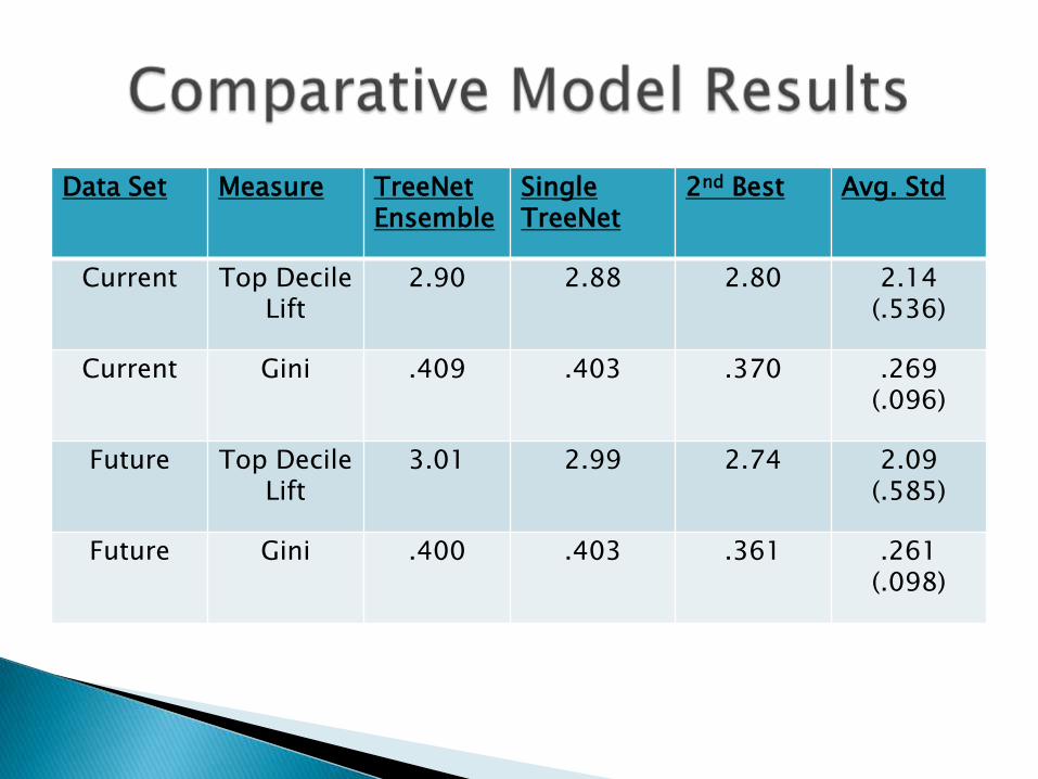
Data Set Measure TreeNetEnsemble

SingleTreeNet

2nd Best Avg. Std

Current Top DecileLift

2.90 2.88 2.80 2.14 (.536)

Current Gini .409 .403 .370 .269 (.096)

Future Top DecileLift

3.01 2.99 2.74 2.09 (.585)

Future Gini .400 .403 .361 .261 (.098)

Single TreeNet model always better than 2nd best entry in field

Ensemble of TreeNets slightly better 3 out of 4 times

Best entries substantially better than the average

In broad telecommunications markets the added accuracy and lift of TreeNet models over alternatives could easily translate into millions of dollars of revenue per year

A modest amount of data preprocessing was undertaken to repair and extend original data

Some missing values could be recorded to “0”

Select non-missing values were recorded to missing

Experiments with missing value handling were conducted, including the addition of missing value indicators to the data◦ CART imputation◦ “All missings together” strategies in decision trees

Missings in a separate node Missings go with non-missing high values Missings go with non-missing low values

TreeNet was key to winning the tournament ◦ Provided considerably greater accuracy and top decile lift than any

other modeling method we tried

A new technology, different than standard boosting, developed by Stanford University Professor Jerome Friedman

Based on the CART® decision tree and thus inherits these characteristics:◦ Automatic feature selection

◦ Invariant with respect to order-preserving transforms of predictors

◦ Immune to outliers

◦ Built-in methods for handling missing values

Based on optimizing an objective function

◦ e.g: Likelihood function or sum of squared errors

Objective function expressed in terms of a target function of the data

◦ The target function is fit as a nonparametric function of the data

◦ The fit optimizes the objective function

Large number of small decision trees used to form the nonparametric estimate

Current implementation allows:

◦ Binary classification

◦ Multinomial classification

◦ Least-squares regression

◦ Least-absolute-deviation regression

◦ M-regression (Huber loss function)

Other objective functions are possible

(Insert equation)

The dependent variable, y, is coded (-1,+1)

The target function, F(x), is ½ the log-odds ratio

F is initialized to the log odds on the full training data set

(Insert equation)◦ Equivalent to fitting data to a constant.

Do not use all training data in any one iteration◦ Randomly sample from training data (we used a 50%

sample)

Compute log-likelihood gradient for each observation◦ (insert equation)

Build a K-node tree to predict G(y,x)◦ K=9 gave the best cross-validated results

◦ Important that trees be much smaller than the size of an optimal single CART tree

Let (insert equations)

Update formula (insert equation)

Repeat until T trees grown

Select the value of m≤T that produces the best fit to the test data

Compute Ymn, a single Newton-Raphson step for Bmn

(insert equation)

Use only a small fraction, p of, Ymn(Bmn=Pymn)

Apply the update formula

(insert equation)

P is called the learning rate, T is the number of trees grown

The product pT is the total learning◦ Holding pT constant, smaller p usually improves model fit to test

data, but can require many trees

Reducing the learning rate tends to slowly increase the optimal amount of total learning

Very low learning rates can require many trees

Our CHURN models used values of p from 0.01 to 0.001

We used total learning of between 6 and 30

All the models used to score the data for the entries used 9-node trees

Our final models used the following three combinations:◦ (p=.001; T=6000; pT=6)◦ (p=.005; T=2500; pT=12.5)◦ (p=.01; T=3000; pT=30)

One entry was a single TreeNet model (p=.01; T=3000; pT=30)◦ In this range all models had almost identical results on test data

◦ The scores were highly correlated (r≥.97)

◦ Within this range, a higher pT was the most important factor

◦ For models with pT=6, the smaller the learning rate the better

(insert table)

(insert graphs)

(insert graph)

(insert graph)

Friedman, J.H. (1999). Stochastic gradient boosting. Stanford: Statistics Department, Stanford University.

Friedman, J.H. (1999). Greedy function approximation: a gradient boosting machine. Stanford: Statistics Department, Stanford University.

Salford Systems (2002) TreeNet™ 1.0 Stochastic Gradient Boosting. San Diego, CA.

Steinberg, D., Cardell, N.S., and Golovnya, M. (2003) Stochastic Gradient Boosting and Restrained Learning. Salford Systems discussion paper.