Chronogram estimation: Penalized Likelihood Approach … · BEAST is a cross-platform program for...

Biology 559R: Introduction to Phylogenetic Comparative Methods

Topics for this week (Feb 3 & 5):

• Chronogram estimation: Penalized Likelihood Approach BEAST

• Presentations of your projects

1

The Anatomy of Trees

• The trees (phylogenies) represent the evolutionary relationships among a group of organisms of interest. • A phylogeny is graph formed by a set of nodes and a set of edges that connect pairs of nodes.


• A node in a phylogeny represents an extant taxon (i.e., a tip or leaf) or a common ancestor for a set of taxa (internal nodes).

Nodes: extant taxon (i.e., a tip or leaf) common ancestor (internal nodes)


• An edge is the part of the phylogeny that connects two nodes (or tips), and is represented by a connecting line (i.e., a branch). We interpret the length of an edge as the amount of evolutionary change or time for transition from an ancestral taxon to a descendant taxon.

Edges or branches (see scale bar for reference)


• The root is the node that represents the last common ancestor of all taxa in the tree. Rooted tree:

A phylogeny without a reference of time

Unrooted tree

A phylogeny where the time is represented by a single direction (bottom-up)

Time-calibrated Phylogenies: Chronograms

• The trees that we have inferred have branch lengths that correspond to the amount of change that has happened on each tip and edge • Most methods and analyses of character evolution are better suited if we use phylogenies whose branch lengths correspond with time (i.e., these trees are ultrametric)

ultrametric tree is one in which the distances from the root to every branch tip are equal.

Chronogram Estimation: A Penalized Likelihood Approach

• We are going to use R and FigTree to estimate an starting chronogram to be input in BEAST. You can use only R for this purpose, but I think it is useful to visualize these fist steps. • Open the Rag1_best_garli.tree from the course website that we estimated using garli

7

to estimate an starting chronogram to be input in BEAST. You can use only R for this purpose, but I think it is useful to visualize

the manipulation menu is not available

Chronogram estimation: A Penalized Likelihood Approach

• We are going to ‘root’ (i.e., give a directionality to) the tree

8

1) click on the branch that we are going to consider that connects to the outgroup

2) the manipulation menu will be activated 3) Then click on the reroot tool


• Our tree will change in shape and then increase the node order (for aesthetics)

9

• Our tree will change in shape and then increase the node order (for aesthetics)


• Then save it in amenable format for R (i.e., newick)

10


• This is how a tree in newick looks like

11

((Polychrus_marmoratus_RAG1_FJ356748:0.04283221,(Hoplocercus_spinosus_RAG1_AY662592:0.01261769,(Morunasaurus_annularis_RAG1_FJ356741:0.011411379999999999,Enyalioides_laticeps_RAG1_GU457971:0.011038409999999999):0.001710199999999995):0.018509200000000003):4.5878E-4,((Dipsosaurus_dorsalis_RAG1_FJ356747:0.03070635,Sauromalus_ater_RAG1_AY662591:0.02422809):0.016886570000000004,((((Uranoscodon_superciliosus_RAG1_JF806215:0.05076097000000001,Stenocercus_guentheri_RAG1_HQ876440:0.04615523):0.012897029999999997,(Gambelia_wislizenii_RAG1_HQ876434:0.010268659999999999,Crotaphytus_collaris_RAG1_FJ356749:0.0119067):0.022629829999999997):0.0021230500000000013,((Anolis_cupreus_RAG1_JN112651:0.027426979999999997,Anolis_equestris_RAG1_JN112653:0.017801500000000005):0.028208580000000004,(Leiocephalus_raviceps_RAG1_FJ356744:0.010438710000000004,Leiocephalus_carinatus_RAG1_AY662598:0.009998069999999998):0.04389986):0.0032812099999999927):0.0023408899999999982,(((Basiliscus_basiliscus_RAG1_JF806202:0.006294059999999997,Basiliscus_plumifrons_RAG1_HM161150:0.0048609599999999975):0.00465753,(Basiliscus_galeritus_RAG1_FJ356743:0.007934999999999998,Corytophanes_cristatus_RAG1_JF806205:0.02278752):0.0027498000000000036):0.029911269999999997,(((Petrosaurus_mearnsi_RAG1_HQ876437:0.0092565,Uta_stansburiana_RAG1_JF806216:0.018854500000000003):0.0077617599999999995,(Phrynosoma_mcallii_RAG1_AY662590:0.01316908,Uma_scoparia_RAG1_JF806214:0.010927510000000001):0.011117379999999996):0.0325743,((Liolaemus_lineomaculatus_RAG1_FJ356740:0.04486896,(Phymaturus_palluma_RAG1_JF806209:0.004616830000000002,Phymaturus_somuncurensis_RAG1_AY662594:0.012232880000000002):0.012305779999999995):0.017839220000000003,((Oplurus_cuvieri_RAG1_JQ073188:0.0071352900000000025,(Chalarodon_madagascariensis_RAG1_JF806204:0.008597300000000002,Chalarodon_madagascariensis_RAG1_JQ073189:0.01288305):0.003126610000000002):0.03292048000000001,(Diplolaemus_darwinii_RAG1_JQ073190:0.014965480000000003,(Pristidactylus_scapulatus_RAG1_JN112660:0.011669610000000004,(Pristidactylus_torquatus_RAG1_JF806210:0.004229379999999998,(Leiosaurus_catamarcensis_RAG1_JF806207:0.0045133099999999995,Urostrophus_gallardoi_RAG1_JN112661:0.020704549999999995):9.772099999999992E-4):0.0010546500000000042):0.008388519999999997):0.012652700000000003):0.0028363099999999947):0.0016280600000000006):7.123299999999971E-4):3.8573999999999553E-4):0.0016100900000000085):4.587799999999978E-4);!


• You can use r8s: http://loco.biosci.arizona.edu/r8s/ See Sanderson (2002) and the r8s manual for further information. However, most of it has been implemented in R. • We are going to use ‘ape’ package to ultrametrize our tree. Load the following package library(ape)!

• Make a working directory and select it as your working. Suggestion: you can also use setwd(). R top menus: Misc>Change Working Directory (select the directory that has our file) • Read our RAG1-phylogeny !rag1_rooted_garli <-read.tree(file = "Rag1_best_garli_rooted.newick")!!

• Let's take a look to our phylogeny !plot(rag1_rooted_garli)!add.scale.bar(x=0, y=0)!

12


13


• Let’s get names of variables in phylogeny names(rag1_rooted_garli)!

• Let’s get tip labels rag1_rooted_garli$tip.label!

• Suggestion: for comparative analyses is better to drop outgroups, so we limit the effect of long branches on the penalized likelihood function that renders our tree ultrametric I will drop one tip, but for the starting BEAST tree we will use the full tree rag1_rooted_garli_no_out <- drop.tip(rag1_rooted_garli, tip ="Polychrus_marmoratus_RAG1_FJ356748")!

• Let's take a look to our tree with and without that tip !par(mfrow=c(1,2))!plot(rag1_rooted_garli)!add.scale.bar(x=0, y=0)!plot(rag1_rooted_garli_no_out)!add.scale.bar(x=0, y=0)!! 14


15


• We can force the tree to be ultrametric using the chronos() function in ‘ape’. • If we don't have a calibration point, we can set the age of the whole tree to "1". First, we need to define the internal function 'makeChronosCalib(rag1_rooted_garli)' of the function 'chronos()'! For relative age chronogram let's fix root at 1 cal_relative <- makeChronosCalib(rag1_rooted_garli, node = "root", age.min = 1, age.max = 1, interactive = FALSE, soft.bounds = FALSE) !!cal_relative!!

For absolute age chronogram, we need to provide a range of possible ages of the reference nodes Notice the change in the parameter to interactive = TRUE and soft.bounds = TRUE !cal_absolute <- makeChronosCalib(rag1_rooted_garli, node = "root", age.min = 1, age.max = 1, interactive = TRUE, soft.bounds = TRUE)# in macs use rigth-click (control + click) on the plot to exit!!

16


17

• For absolute age chronogram, we need to provide a range of possible ages of the reference nodes !cal_absolute <- makeChronosCalib(rag1_rooted_garli, node = "root", age.min = 1, age.max = 1, interactive = TRUE, soft.bounds = TRUE)# in macs use rigth-click (control + click) on the plot to exit!!

(node number: 49): younger age is 15 and older age 35


root (node number: 34): younger age is 55 and older age 76


18

• For absolute age chronogram, we need to provide a range of possible ages of the reference nodes !cal_absolute <- makeChronosCalib(rag1_rooted_garli, node = "root", age.min = 1, age.max = 1, interactive = TRUE, soft.bounds = TRUE)# in macs use rigth-click (control + click) on the plot to exit!!

(node number: 49): younger age is 15 and older age 35 (node number: 59): younger age is 40 and older age 62 root (node number: 34): younger age is 55 and older age 76


• Both cal_relative and cal_absolute are data frames, so you can modify these data without the interactive mode cal_relative!cal_absolute!!

• Let's estimate our chronogram using Penalized Likelihood and Maximum Likelihood. We need to select a method, I prefer a relaxed clock model to account for heterogeneity among branches. • We also need to select a smoothing parameter lambda (see Sanderson, 2002) If lambda = 0, then the parametric component dominates and rates vary as much as possible among branches, whereas for increasing values of lambda, the variation in the rates are smoother and tend to a clock-like model (same rate for all branches) • However, I prefer BEAST for my chronogram estimation given that it is more parametrized and used the actual data to estimate the chronogram. So, you can pick an arbitrary lambda or test of different lambdas for this chronogram (This is just a starting tree for our BEAST analysis)

19


• Relative age chronogram with three smoothing parameters rag1_chrono_rel_garli_lambda_0 <- chronos(rag1_rooted_garli, model = "relaxed", lambda = 0, calibration = cal_relative) !rag1_chrono_rel_garli_lambda_0_1 <- chronos(rag1_rooted_garli, model = "relaxed", lambda = 0.1, calibration = cal_relative) !rag1_chrono_rel_garli_lambda_1_0 <- chronos(rag1_rooted_garli, model = "relaxed", lambda = 1.0, calibration = cal_relative) !!rag1_chrono_abs_garli_lambda_0 <- chronos(rag1_rooted_garli, model = "relaxed", lambda = 0, calibration = cal_absolute) !rag1_chrono_abs_garli_lambda_0_1 <- chronos(rag1_rooted_garli, model = "relaxed", lambda = 0.1, calibration = cal_absolute) !rag1_chrono_abs_garli_lambda_1_0 <- chronos(rag1_rooted_garli, model = "relaxed", lambda = 1.0, calibration = cal_absolute) !!

• Check the 'Penalised log-lik' values, the you want the largest likelihood; i.e., largest likelihood or smallest negative log-likelihood. Negative numbers are OK. A log-likelihood of -2 is better than -4. The best in this case corresponds to the lambda = 0 (i.e., Penalised log-lik = -3.885571) !

20


• After the calculations are done, we can write the trees in newick format for future use. write.tree (rag1_chrono_rel_garli_lambda_0, file ="rag1_chrono_rel_garli_lambda_0.newick")!write.tree (rag1_chrono_rel_garli_lambda_0_1, file ="rag1_chrono_rel_garli_lambda_0_1.newick")!write.tree (rag1_chrono_rel_garli_lambda_1_0, file ="rag1_chrono_rel_garli_lambda_1_0.newick")!!write.tree (rag1_chrono_abs_garli_lambda_0, file ="rag1_chrono_abs_garli_lambda_0.newick")!write.tree (rag1_chrono_abs_garli_lambda_0_1, file ="rag1_chrono_abs_garli_lambda_0_1.newick")!write.tree (rag1_chrono_abs_garli_lambda_1_0, file ="rag1_chrono_abs_garli_lambda_1_0.newick")!!

• Let's check that our trees are ultrametric is.ultrametric(rag1_rooted_garli)!is.ultrametric(rag1_chrono_rel_garli_lambda_0)!is.ultrametric(rag1_chrono_rel_garli_lambda_0_1)!is.ultrametric(rag1_chrono_rel_garli_lambda_1_0)!is.ultrametric(rag1_chrono_abs_garli_lambda_0)!is.ultrametric(rag1_chrono_abs_garli_lambda_0_1)!is.ultrametric(rag1_chrono_abs_garli_lambda_1_0)!!

21


22

Chronogram estimation: BEAST

23

• One of the most widely used software to estimate chronograms and most recently species trees Drummond AJ, Suchard MA, Xie D & Rambaut A (2012) Bayesian phylogenetics with BEAUti and the BEAST 1.7 Molecular Biology And Evolution 29: 1969-1973 http://beast.bio.ed.ac.uk/ From the authors: BEAST is a cross-platform program for Bayesian analysis of molecular sequences using MCMC. It is entirely orientated towards rooted, time-measured phylogenies inferred using strict or relaxed molecular clock models. It can be used as a method of reconstructing phylogenies but is also a framework for testing evolutionary hypotheses without conditioning on a single tree topology. BEAST uses MCMC to average over tree space, so that each tree is weighted proportional to its posterior probability. We include a simple to use user-interface program for setting up (BEAUTi) standard analyses and a suit of programs for analysing the results.


24

• This software has detailed manuals and tutorials: http://beast.bio.ed.ac.uk/tutorials • After installation, you will also require the extensive set of auxiliary programs. Most of them are included in the BEAST package, but others require independent installation. Bayesian Evolutionary Analysis Utility (BEAUti): GUI application for the preparation of the BEAST XML files. LogCombiner: Program that allows you to combine log and tree files from multiple independent runs of BEAST. TreeAnnotator: Program that assists you in summarizing the information from a sample of trees produced by BEAST. Tracer: is graphical tool for visualization and diagnostics of MCMC output. It can read output files from MrBayes and BEAST (Not in BEAST package): http://tree.bio.ed.ac.uk/software/tracer/ FigTree: You know this one.


25

• This is very important, you need to install BEAGLE BEAGLE is a high-performance library that can perform the core calculations at the heart of most Bayesian and Maximum Likelihood phylogenetics package. It can make use of highly-parallel processors such as those in 3D graphics boards found in many PCs. http://beast.bio.ed.ac.uk/BEAGLE MACs: https://code.google.com/p/beagle-lib/wiki/MacInstallInstructions Windows: https://code.google.com/p/beagle-lib/wiki/WindowsInstallInstructions

Preparing run for BEAST using a starting tree

26

• You need to create a folder with a nexus file with the sequences and the chronogram that we estimated using ‘ape’. Folder: RAG1_BEST


27

• Edit and add the chronogram at the end of the nexus file (I have added the edited file to the courser website): RAG1_nucleotide_chrono.nex

Our chronogram

Partitions by codon (if you have multiple genes)


28

• Open BEAUti v1.8.1 and import the nexus file with chronogram


29

• Open BEAUti v1.8.1 and import the nexus file with chronogram

Our data file

Our starting chronogram and partitions (e.g., genes, codon positions)


30

• We are going to change the partitions defaults for codon positions in a single gene, but you can do the same procedure for multiple genes. You need to do the following to allow to run a partitioned dataset: 1) On the partitions tab select all partitions or genes 2) We like to analyze each partition/gene under separate substitutions models, while assuming the clock and tree are linked Highlight all three partitions/genes Unlink Subst. Models 3) Rename Partition Clock Model. Changes are done by highlighting all partitions Highlight all three partitions/genes Link Clock Models Rename this to Rag1_clock 4) Rename Partition Tree. Changes are done by highlighting all partitions Highlight all three genes Link Trees Rename this to Rag1_tree


31

• After all of these changes you should have something like this:


32

• We will create the calibration nodes and identifying internal nodes in the Taxa tab Notice: If not enforced monophyletic, then it is possible to define a node using a pair of descendant taxa and use the name of the node corresponding to their MRCA (most recent common ancestor) to define calibration times. This procedure will reduced the time editing the xml BEAST file

Click of + to start defining groups that will used to do calibrations

33

• We are going to use the same calibration nodes that we did in the Penalized Likelihood Approach!!



root (node number: 34): younger age is 55 and older age 76


34




35




36

• Not necessary to worry about Tips (do not click) • Not necessary to worry about Traits tab (do not click) • On the Sites tab will select the substitution models for each partition/gene. We did this part for the entire RAG1 gene in jModelTest, but not for each of its codon positions. For this exercise, we will assume that each position has a GTR+G+I model. Notice the limited number of models


37

• On the Clocks tab will estimate the clock (click on Estimate) The model will be ‘Lognormal relaxed clock (Uncorrelated)’ which is fit for more distantly related taxa and low taxon sampling.


38

• On the Trees tab will we are going to select a tree prior and starting trees Tree Prior -> Speciation: Birth-Death Incomplete Sampling (also Yule process is useful) Random starting tree if you do not have an starting tree


Speciation: Birth-Death Incomplete Sampling (also Yule process is useful)

39

• Not necessary to worry about States (do not click) • On the Priors tab will input some a priori information to allow us find our time calibrated chronogram


will input some a priori information to allow us find our time calibrated

Node upper and lower ages

parameters for the clock model

40

• Nodes with an upper and lower within an uniform distribution


41

• Parameter for the clock model


I trust the theoreticians and this values for this prior seems to work well

42

• On the tab Operators left them as they are, the software is going ‘Auto optimize’ while searching for the optimal chronogram. • On the MCMC tab will like to have a really long chain > 90 million (depends on the computational disponibility and time). • I usually run at least 4 independent starts (based on random numbers)


43

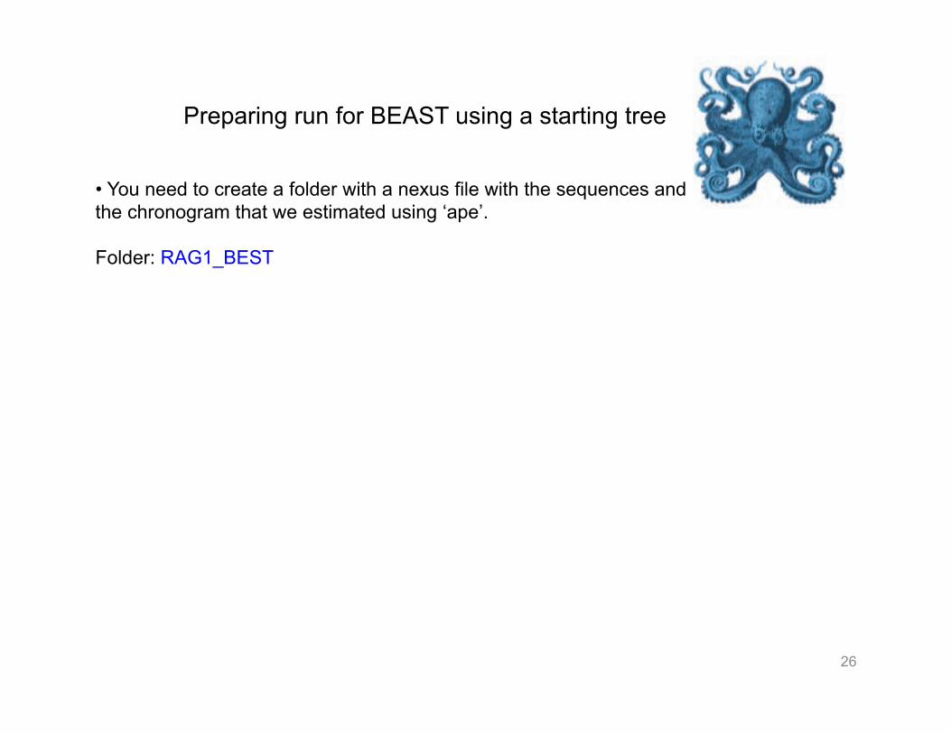
• Generate the BEAST file. But, DO NOT CLOSE BEUTi, this will allow you correct mistakes easily in case something needs a quick fix • A tab about un changed defaults priors will appear, just click ‘Continue’


44

• BEAST has tends to split long trees into pieces that need to put in a single line: It should be like this: • During a test run I found that one of the lower bound of the uniform distribution of the Corytophanidae node was to high and I have to fix it to a lower value. It is very likely that you will have to review the BEAUTi file for such changes.

Fixing the BEAUTi file

45

• If you made a good job, then BEAST will run for a long time and will produce several intermediate files. I recommend to create a folder for each run and have at least 4 independent starts. • The same xml file will run in the cluster, so check that it runs in your computer before you send it to the cluster • Click on BEAST v1.8.1, select you xml file and run. • For independent starts, change the Random Number Seed

Running BEAST

46

• Check the performance of the run and wait until it finishes

Running BEAST

47

• The run will finish with a report about the operators

Running BEAST

48

• Open Tracer and explore the results of the course website: RAG1_nucleotide_chrono.log.zip

BEAST: Visualizing the results in Tracer

49

From the Manual: On the left hand side is a list of the different quantities that BEAST has logged. There are traces for the posterior (this is the log of the product of the tree likelihood and the prior probabilities), and the continuous parameters. Selecting a trace on the left brings up analyses for this trace on the right hand side depending on tab that is selected.

• Open Tracer and explore the results of: RAG1_nucleotide_chrono.log


50

From the Manual: On the left hand side is a list of the different quantities that BEAST has logged. the posterior (this is the log of the product of the tree likelihood and the prior probabilities), and the continuous parameters. Burn-In: We need to discard early very bad estimates that usually do not add information to our parameter estimation. These wrong estimates are usually visualized using the Trace Tab

Burn-In:

• Open Tracer and explore the results of: RAG1_nucleotide_chrono.log


51

• Tracer will display summary statistics (e.g., means) and in the estimates in each parameter as the run progresses (graph). • We are interested in Effective Sample Size (ESS). This value indicates the size of a set of independent data points with the same information. • If ESS is good if it is high enough (i.e., > 100) it will also be indicated in black. • A low ESS (e.g., < 100) means that even though we may have sampled many data points, our search is rejecting most of its proposals (e.g., node ages) and thus may not represent the posterior distribution well. Other reason is that the proposals it accepts are all very close together so that it is not moving freely across the surface. • Tracer will color Effective Sample Size (ESS) statistic under 100 as RED indicating a run which is too short. We need to run longer our chains (as many times the lowest ESS to get > 100 ESS for that parameter: if ESS = 25 you should run > 4 times the chain). • It is suggested to have ESS > 200 to be confident in our estimates. For more information read:http://beast.bio.ed.ac.uk/analysing-beast-output

BEAST: Visualizing the results

52

• Let’s explore the results of our nodes that we assigned calibration dates • This BEAST search look in general good, so lets estimate our summary chronogram.

BEAST: Visualizing the results

53

• If you have more than 1 run, you need to be combined the tree and log files using LogCombiner v1.8.1 (see Manual). • Use Tracer to determine if your total runs are long enough to get a high ESS • Then, open TreeAnnotator v1.8.1 and select the file from the course website: RAG1_nucleotide_chrono.trees.zip to create a summary tree for the graphs make sure: 1) to define the number of trees to burn-in with at least stationary posterior, in our case 5000000 2) posterior probability limit at 0.0 3) set to maximum clade credibility tree 4) set to Mean or Median heights

BEAST: Summary Tree

54

BEAST: Summary Tree

55

BEAST: Summary Tree

We will get in our folder the annotated tree: RAG1_nucleotide_chrono_summary.tre We can now visualize our chronogram in FigTree and this can be used for comparative analyses

• We can explore this tree or the one in the course website: RAG1_nucleotide_chrono_summary.tre and see the nodal 95% HPD (highest posterior density interval) which represents the most compact interval on the selected parameter that contains 95% of the posterior probability. • These 95% HPD can be thought of as a Bayesian analog to a confidence interval.

56

BEAST: Summary Tree

57

BEAST: Summary Tree

58

Presentations

• This next Thursday (Feb 5th) • You have 5 minutes (3 min for presentation and 2 min for questions) • You will need to send me or bring a pdf of your presentation (so I put it in my computer) • You will need to give me an abstract of your project: Title: 150 characters (including spaces) Text: 300 words maximum for your abstract. This should include: A brief background introduction Your main question or hypothesis Summary or names of comparative methods that you plan to use Your expected results

Chronogram estimation: Penalized Likelihood Approach … · BEAST is a cross-platform program for...

Documents

Transcript of Chronogram estimation: Penalized Likelihood Approach … · BEAST is a cross-platform program for...