Christopher F Baum - NCER · Christopher F Baum (BC / DIW) Using Stata NCER/QUT, 2014 11 / 138...
138
Using Stata for data management and reproducible research Christopher F Baum Boston College and DIW Berlin NCER, Queensland University of Technology, March 2014 Christopher F Baum (BC / DIW) Using Stata NCER/QUT, 2014 1 / 138
Transcript of Christopher F Baum - NCER · Christopher F Baum (BC / DIW) Using Stata NCER/QUT, 2014 11 / 138...

Using Stata for data managementand reproducible research
Christopher F Baum
Boston College and DIW Berlin
NCER, Queensland University of Technology, March 2014
Christopher F Baum (BC / DIW) Using Stata NCER/QUT, 2014 1 / 138

Overview of the Stata environment
Overview of the Stata environment
Stata is a full-featured statistical programming language for Windows,Mac OS X, Unix and Linux. It can be considered a “stat package,” likeSAS, SPSS, RATS, or eViews.
Stata is available in several versions: Stata/IC (the standard version),Stata/SE (an extended version) and Stata/MP (for multiprocessing).The major difference between the versions is the number of variablesallowed in memory, which is limited to 2,047 in standard Stata/IC, butcan be up to 32,767 in Stata/SE or Stata/MP. The number ofobservations in any version is limited only by your computer’s memory.
Christopher F Baum (BC / DIW) Using Stata NCER/QUT, 2014 2 / 138

Overview of the Stata environment
Stata/SE relaxes the Stata/IC constraint on the number of variables,while Stata/MP is the multiprocessor version, capable of utilizing 2, 4,8, 16... processors available on a single computer. Stata/IC will meetmost users’ needs; if you have access to Stata/SE or Stata/MP, youcan use that program to create a subset of a large survey dataset withfewer than 2,047 variables. Stata runs on all 64-bit operating systems,and can access larger datasets on a 64-bit OS, which can address alarger memory space.
All versions of Stata provide the full set of features and commands:there are no special add-ons or ‘toolboxes’. Each copy of Stataincludes a complete set of manuals (over 11,000 pages) in PDFformat, hyperlinked to the on-line help.
Christopher F Baum (BC / DIW) Using Stata NCER/QUT, 2014 3 / 138
Overview of the Stata environment
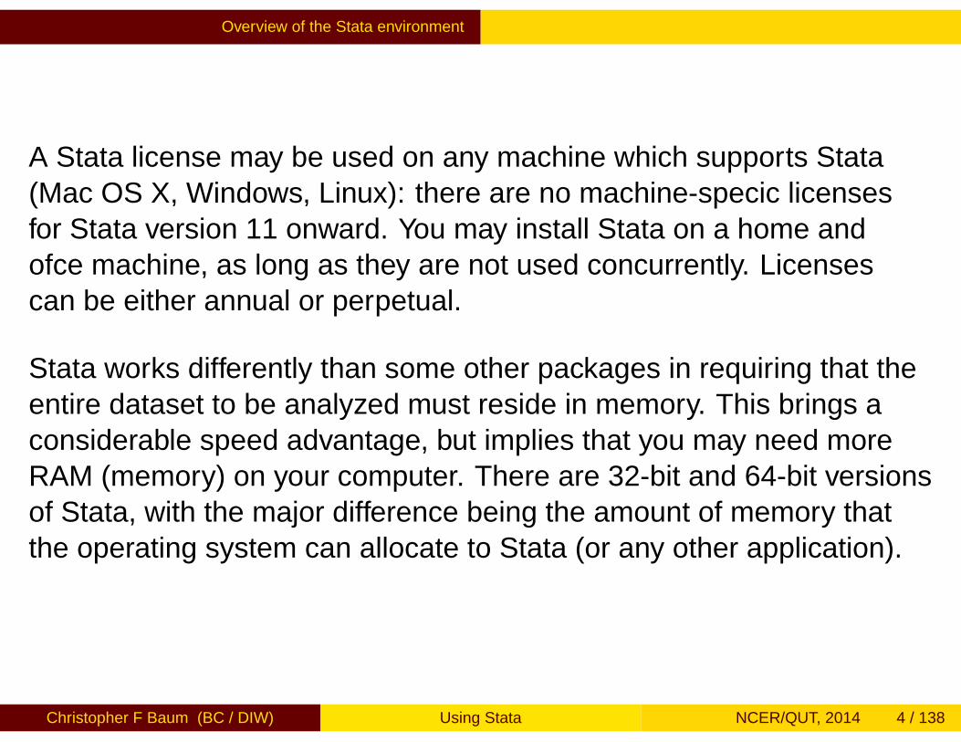
A Stata license may be used on any machine which supports Stata(Mac OS X, Windows, Linux): there are no machine-specific licensesfor Stata version 11 onward. You may install Stata on a home andoffice machine, as long as they are not used concurrently. Licensescan be either annual or perpetual.
Stata works differently than some other packages in requiring that theentire dataset to be analyzed must reside in memory. This brings aconsiderable speed advantage, but implies that you may need moreRAM (memory) on your computer. There are 32-bit and 64-bit versionsof Stata, with the major difference being the amount of memory thatthe operating system can allocate to Stata (or any other application).
Christopher F Baum (BC / DIW) Using Stata NCER/QUT, 2014 4 / 138
Overview of the Stata environment
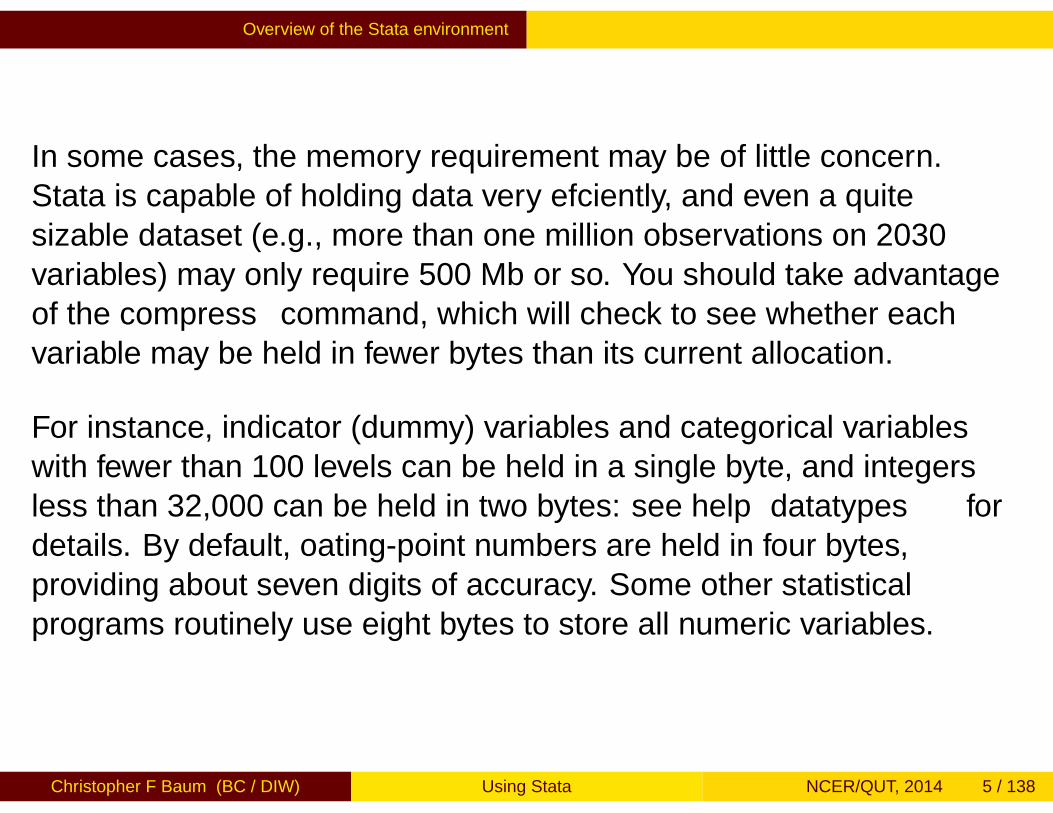
In some cases, the memory requirement may be of little concern.Stata is capable of holding data very efficiently, and even a quitesizable dataset (e.g., more than one million observations on 20–30variables) may only require 500 Mb or so. You should take advantageof the compress command, which will check to see whether eachvariable may be held in fewer bytes than its current allocation.
For instance, indicator (dummy) variables and categorical variableswith fewer than 100 levels can be held in a single byte, and integersless than 32,000 can be held in two bytes: see help datatypes fordetails. By default, floating-point numbers are held in four bytes,providing about seven digits of accuracy. Some other statisticalprograms routinely use eight bytes to store all numeric variables.
Christopher F Baum (BC / DIW) Using Stata NCER/QUT, 2014 5 / 138
Overview of the Stata environment
The memory available to Stata may be considerably less than theamount of RAM installed on your computer. If you have a 32-bitoperating system, it does not matter that you might have 4 Gb or moreof RAM installed; Stata will only be able to access about 1 Gb,depending on other processes’ demands.
To make most effective use of Stata with large datasets, you shoulduse a computer with a 64-bit operating system. Stata will automaticallyinstall a 64-bit version of the program if it is supported by the operatingsystem. All Linux, Unix and Mac OS X computers today come with64-bit operating systems.
Christopher F Baum (BC / DIW) Using Stata NCER/QUT, 2014 6 / 138
Overview of the Stata environment Portability
Stata is eminently portable, and its developers are committed tocross-platform compatibility. Stata runs the same way on Windows,Mac OS X, Unix, and Linux systems. The only platform-specificaspects of using Stata are those related to native operating systemcommands: e.g. is the file to be accessed
C:\Stata\StataData\myfile.dtaor/users/baum/statadata/myfile.dta
Perhaps unique among statistical packages, Stata’s binary data filesmay be freely copied from one platform to any other, or even accessedover the Internet from any machine that runs Stata. You may storeStata’s binary datafiles on a webserver (HTTP server) and open themon any machine with access to that server.
Christopher F Baum (BC / DIW) Using Stata NCER/QUT, 2014 7 / 138
Overview of the Stata environment Stata’s user interface
Stata’s user interface
Stata has traditionally been a command-line-driven package thatoperates in a graphical (windowed) environment. Stata version 11(released June 2009), version 12 (released July 2011) and version 13(released June 2013) contain a graphical user interface (GUI) forcommand entry via menus and dialogs. Stata may also be used in acommand-line environment on a shared system (e.g., a Unix server) ifyou do not have a graphical interface to that system.
A major advantage of Stata’s GUI system is that you always have theoption of reviewing the command that has been entered in Stata’sReview panel. Thus, you may examine the syntax, revise it in theCommand panel and resubmit it. You may find that this is a moreefficient way of using the program than relying wholly on dialogs.
Christopher F Baum (BC / DIW) Using Stata NCER/QUT, 2014 8 / 138
Overview of the Stata environment Stata’s user interface
Stata version 13, default screen appearance:
Christopher F Baum (BC / DIW) Using Stata NCER/QUT, 2014 9 / 138

Overview of the Stata environment Stata’s user interface
The Toolbar contains icons that allow you to Open and Save files, Printresults, control Logs, and manipulate windows. Some very importanttools allow you to open the Do-File Editor, the Data Editor and the DataBrowser.
The Data Editor and Data Browser present you with a spreadsheet-likeview of the data, no matter how large your dataset may be. TheDo-File editor, as we will discuss, allows you to construct a file of Statacommands, or “do-file”, and execute it in whole or in part from theeditor.
Christopher F Baum (BC / DIW) Using Stata NCER/QUT, 2014 10 / 138
Overview of the Stata environment Stata’s user interface
The foot of the screen also contains an important piece of information:the Current Working Directory, or cwd. In the screenshot, it is listed ascfbaum > Documents > . The cwd is the directory to which anyfiles created in your Stata session will be saved. Likewise, if you try toopen a file and give its name alone, it is assumed to reside in the cwd.If it is in another location, you must change the cwd [File→ChangeWorking Directory] or qualify its name with the directory in which itresides.
You generally will not want to locate or save files in the default cwd. Acommon strategy is to set up a directory for each project or task in aconvenient location in the filesystem and change the cwd to thatdirectory when working on that task. This can be automated in ado-file with the cd command.
Christopher F Baum (BC / DIW) Using Stata NCER/QUT, 2014 11 / 138
Overview of the Stata environment Stata’s user interface
There are several panels in the default interface: the Review, Results,Command, Variables and Properties panels. You may alter theappearance of any panel in the GUI using the Preferences→Generaldialog, and make those changes on a temporary or permanent basis.
As you might expect, you may type commands in the Command panel.You may only enter one command in that panel, so you should not trypasting a list of several commands. When a command isexecuted—with or without error—it appears in the Review panel, andthe results of the command (or an error message) appears in theResults panel. You may click on any command in the Review paneland it will reappear in the Command panel, where it may be edited andresubmitted.
Christopher F Baum (BC / DIW) Using Stata NCER/QUT, 2014 12 / 138
Overview of the Stata environment Stata’s user interface
Once you have loaded data into the program, the Variables panel willbe populated with information on each variable, as you can see in theexample. That information includes the variable name, its label (if any),its type and its format. This is a subset of information available fromthe describe command.
Let’s look at the interface after I have loaded one of the datasetsprovided with Stata, uslifeexp, with the sysuse command andgiven the describe and summarize commands:
Christopher F Baum (BC / DIW) Using Stata NCER/QUT, 2014 13 / 138
Overview of the Stata environment Stata’s user interface
Christopher F Baum (BC / DIW) Using Stata NCER/QUT, 2014 14 / 138

Overview of the Stata environment Stata’s user interface
Notice that the three commands are listed in the Review panel. If anyhad failed, the _rc column would contain a nonzero number, in red,indicating the error code.
The Variables panel contains the list of variables and their labels.
The Results panel shows the effects of summarize: for each variable,the number of observations, their mean, standard deviation, minimumand maximum. If there were any string variables in the dataset, theywould be listed as having zero observations.
Christopher F Baum (BC / DIW) Using Stata NCER/QUT, 2014 15 / 138
Overview of the Stata environment Stata’s user interface
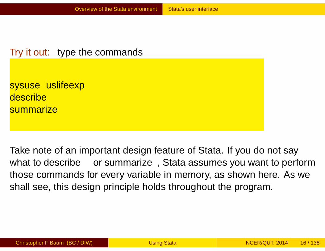
Try it out: type the commands
sysuse uslifeexpdescribesummarize
Take note of an important design feature of Stata. If you do not saywhat to describe or summarize, Stata assumes you want to performthose commands for every variable in memory, as shown here. As weshall see, this design principle holds throughout the program.
Christopher F Baum (BC / DIW) Using Stata NCER/QUT, 2014 16 / 138
Overview of the Stata environment Using the Do-File Editor
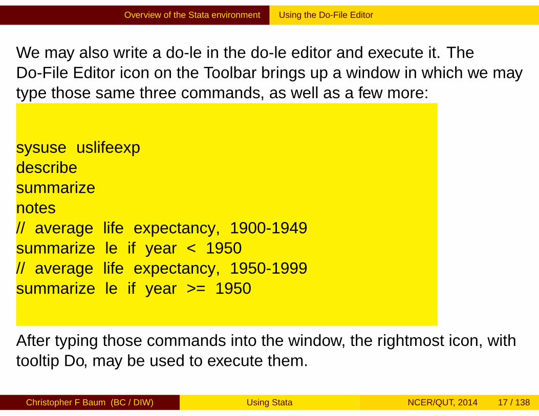
We may also write a do-file in the do-file editor and execute it. TheDo-File Editor icon on the Toolbar brings up a window in which we maytype those same three commands, as well as a few more:
sysuse uslifeexpdescribesummarizenotes// average life expectancy, 1900-1949summarize le if year < 1950// average life expectancy, 1950-1999summarize le if year >= 1950
After typing those commands into the window, the rightmost icon, withtooltip Do, may be used to execute them.
Christopher F Baum (BC / DIW) Using Stata NCER/QUT, 2014 17 / 138

Overview of the Stata environment Using the Do-File Editor
Christopher F Baum (BC / DIW) Using Stata NCER/QUT, 2014 18 / 138
Overview of the Stata environment Using the Do-File Editor
In this do-file, I have included the notes command to display the notessaved with the dataset, and included two comment lines. There areseveral styles of comments available. In this style, anything on a linefollowing a double slash (//) is ignored. You may also place an asterisk(*) on the left margin to indicate a comment, or surround severalcomment lines in a do-file with the /* . . . */ notation.
If a command is too long to fit comfortably on a single line, you maycontinue it on successive lines by placing a triple slash (///) at theend of each line.
You may use the other icons in the Do-File Editor window to save yourdo-file (to the cwd or elsewhere), print it, or edit its contents. You mayalso select a portion of the file with the mouse and execute only thosecommands.
Christopher F Baum (BC / DIW) Using Stata NCER/QUT, 2014 19 / 138

Overview of the Stata environment Using the Do-File Editor
Christopher F Baum (BC / DIW) Using Stata NCER/QUT, 2014 20 / 138
Overview of the Stata environment Using the Do-File Editor
Try it out: use the Do-File Editor to save and reopen the do-fileS1.1.do, and run the file.
Try selecting only those last four lines and run those commands.
Christopher F Baum (BC / DIW) Using Stata NCER/QUT, 2014 21 / 138
Overview of the Stata environment The help system
The rightmost menu on the menu bar is labeled Help. From that menu,you can search for help on any command or feature. The HelpBrowser, which opens in a Viewer window, provides hyperlinks, in blue,to additional help pages. At the foot of each help screen, there arehyperlinks to the full manuals, which are accessible in PDF format.The links will take you directly to the appropriate page of the manual.
You may also search for help at the command line with helpcommand. But what if you don’t know the exact command name?Then you may use the search command, which may be followed byone or several words.
Christopher F Baum (BC / DIW) Using Stata NCER/QUT, 2014 22 / 138
Overview of the Stata environment The help system
Results from search are presented in a Viewer window. Thosecommands will present results from a keyword database and from theInternet: for instance, FAQs from the Stata website, articles in theStata Journal and Stata Technical Bulletin, and downloadable routinesfrom the SSC Archive (about which more later) and user sites.
Try it out: when you are connected to the Internet, type the commands
search baum, ausearch baum
Note the hyperlinks that appear on URLs for the books and journalarticles, and on the individual software packages (e.g., st0030_3,archlm).
Christopher F Baum (BC / DIW) Using Stata NCER/QUT, 2014 23 / 138

Overview of the Stata environment Stata’s update facility
Stata’s update facility
One of Stata’s great strengths is that it can be updated over theInternet. Stata is actually a web browser, so it may contact Stata’s webserver and enquire whether there are more recent versions of eitherStata’s executable (the kernel) or the ado-files. This enables Stata’sdevelopers to distribute bug fixes, enhancements to existingcommands, and even entirely new commands during the lifetime of agiven major release (including ‘dot-releases’ such as Stata 12.1).
Updates during the life of the version you own are free. You need onlyhave a licensed copy of Stata and access to the Internet (which maybe by proxy server) to check for and, if desired, download the updates.
Christopher F Baum (BC / DIW) Using Stata NCER/QUT, 2014 24 / 138

Overview of the Stata environment Extensibility
Extensibility of official Stata
Another advantage of the command-line driven environment involvesextensibility: the continual expansion of Stata’s capabilities. Acommand, to Stata, is a verb instructing the program to perform someaction.
Commands may be “built in” commands—those elements sofrequently used that they have been coded into the “Stata kernel.” Arelatively small fraction of the total number of official Stata commandsare built in, but they are used very heavily.
Christopher F Baum (BC / DIW) Using Stata NCER/QUT, 2014 25 / 138
Overview of the Stata environment Extensibility
The vast majority of Stata commands are written in Stata’s ownprogramming language–the “ado-file” language. If a command is notbuilt in to the Stata kernel, Stata searches for it along the adopath.Like the PATH in Unix, Linux or DOS, the adopath indicates theseveral directories in which an ado-file might be located. This impliesthat the “official” Stata commands are not limited to those coded intothe kernel.
Try it out: give the
adopath
command in Stata.
Christopher F Baum (BC / DIW) Using Stata NCER/QUT, 2014 26 / 138
Overview of the Stata environment Extensibility
If Stata’s developers tomorrow wrote a new command named “foobar”,they would make two files available on their web site: foobar.ado(the ado-file code) and foobar.sthlp (the associated help file). Bothare ordinary, readable ASCII text files. These files should be producedin a text editor, not a word processing program.
Christopher F Baum (BC / DIW) Using Stata NCER/QUT, 2014 27 / 138

Overview of the Stata environment Extensibility
The importance of this program design goes far beyond the limits ofofficial Stata. Since the adopath includes both Stata directories andother directories on your hard disk (or on a server’s filesystem), youmay acquire new Stata commands from a number of web sites. TheStata Journal (SJ), a quarterly peer-reviewed journal, is the primarymethod for distributing user contributions. Between 1991 and 2001,the Stata Technical Bulletin played this role, and a complete set ofissues of the STB are available on line at the Stata website.
Christopher F Baum (BC / DIW) Using Stata NCER/QUT, 2014 28 / 138
Overview of the Stata environment Extensibility
The SJ is a subscription publication (articles more than three years oldfreely downloadable), but the ado- and sthlp-files may be freelydownloaded from Stata’s web site. The Stata help commandaccesses help on all installed commands; the Stata search commandwill locate commands that have been documented in the STB and theSJ, and with one click you may install them in your version of Stata.Help for these commands will then be available in your own copy.
Christopher F Baum (BC / DIW) Using Stata NCER/QUT, 2014 29 / 138
Overview of the Stata environment Extensibility
User extensibility: the SSC archive
But this is only the beginning. Stata users worldwide participate in theStataList listserv, and when a user has written and documented a newgeneral-purpose command to extend Stata functionality, theyannounce it on the StataList listserv (to which you may freelysubscribe: see Stata’s web site).
Since September 1997, all items posted to StataList (over 1,500)have been placed in the Boston College Statistical SoftwareComponents (SSC) Archive in RePEc (Research Papers inEconomics), available from IDEAS (http://ideas.repec.org) andEconPapers (http://econpapers.repec.org).
Christopher F Baum (BC / DIW) Using Stata NCER/QUT, 2014 30 / 138

Overview of the Stata environment Extensibility
Any component in the SSC archive may be readily inspected with aweb browser, using IDEAS’ or EconPapers’ search functions, and ifdesired you may install it with one command from the archive fromwithin Stata. For instance, if you know there is a module in the archivenamed mvsumm, you could use ssc describe mvsumm to learnmore about it, and ssc install mvsumm to install it if you wish.Anything in the archive can be accessed via Stata’s ssc command:thus ssc describe mvsumm will locate this module, and make itpossible to install it with one click.
Windows users should not attempt to download the materials from aweb browser; it won’t work.
Christopher F Baum (BC / DIW) Using Stata NCER/QUT, 2014 31 / 138
Overview of the Stata environment Extensibility
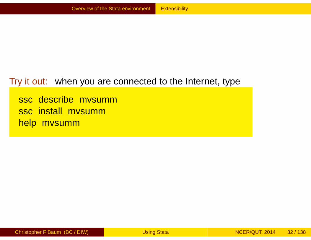
Try it out: when you are connected to the Internet, type
ssc describe mvsummssc install mvsummhelp mvsumm
Christopher F Baum (BC / DIW) Using Stata NCER/QUT, 2014 32 / 138

Overview of the Stata environment Extensibility
The command ssc new lists, in the Stata Viewer, all SSC packagesthat have been added or modified in the last month. You may click ontheir names for full details. The command ssc hot reports on themost popular packages on the SSC Archive.
The Stata command adoupdate checks to see whether all packagesyou have downloaded and installed from the SSC archive, the StataJournal, or other user-maintained net from... sites are up to date.adoupdate alone will provide a list of packages that have beenupdated. You may then use adoupdate, update to refresh yourcopies of those packages, or specify which packages are to beupdated.
Christopher F Baum (BC / DIW) Using Stata NCER/QUT, 2014 33 / 138
Overview of the Stata environment Extensibility
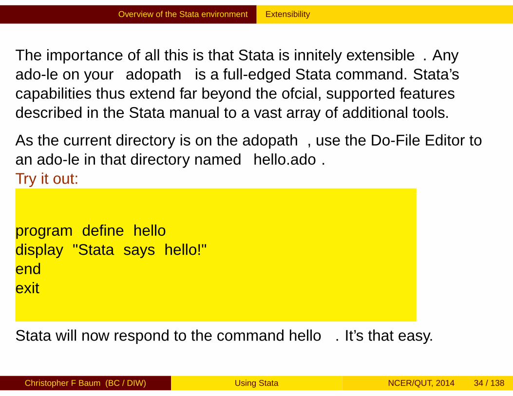
The importance of all this is that Stata is infinitely extensible. Anyado-file on your adopath is a full-fledged Stata command. Stata’scapabilities thus extend far beyond the official, supported featuresdescribed in the Stata manual to a vast array of additional tools.
As the current directory is on the adopath, use the Do-File Editor toan ado-file in that directory named hello.ado.Try it out:
program define hellodisplay "Stata says hello!"endexit
Stata will now respond to the command hello. It’s that easy.
Christopher F Baum (BC / DIW) Using Stata NCER/QUT, 2014 34 / 138
Working with the command line Stata command syntax
Stata command syntax
Let us consider the form of Stata commands. One of Stata’s greatstrengths, compared with many statistical packages, is that itscommand syntax follows strict rules: in grammatical terms, there areno irregular verbs. This implies that when you have learned the way afew key commands work, you will be able to use many more withoutextensive study of the manual or even on-line help.
Christopher F Baum (BC / DIW) Using Stata NCER/QUT, 2014 35 / 138
Working with the command line Stata command syntax
The fundamental syntax of all Stata commands follows a template. Notall elements of the template are used by all commands, and someelements are only valid for certain commands. But where an elementappears, it will appear in the same place, following the same grammar.
Like Unix or Linux, Stata is case sensitive. Commands must be givenin lower case. For best results, keep all variable names in lower caseto avoid confusion.
Christopher F Baum (BC / DIW) Using Stata NCER/QUT, 2014 36 / 138
Working with the command line Command template
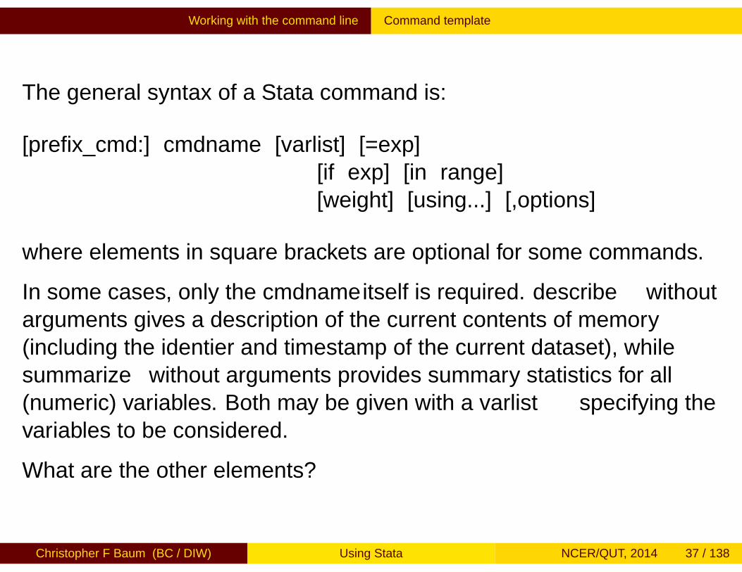
The general syntax of a Stata command is:
[prefix_cmd:] cmdname [varlist] [=exp][if exp] [in range][weight] [using...] [,options]
where elements in square brackets are optional for some commands.
In some cases, only the cmdname itself is required. describe withoutarguments gives a description of the current contents of memory(including the identifier and timestamp of the current dataset), whilesummarize without arguments provides summary statistics for all(numeric) variables. Both may be given with a varlist specifying thevariables to be considered.
What are the other elements?
Christopher F Baum (BC / DIW) Using Stata NCER/QUT, 2014 37 / 138
Working with the command line The varlist
The varlist
varlist is a list of one or more variables on which the command is tooperate: the subject(s) of the verb. Stata works on the concept of asingle set of variables currently defined and contained in memory,each of which has a name. As the describe command will show you,each variable has a data type (various sorts of integers and reals, andstring variables of a specified maximum length). The varlist specifieswhich of the defined variables are to be used in the command.
Christopher F Baum (BC / DIW) Using Stata NCER/QUT, 2014 38 / 138
Working with the command line The varlist
The order of variables in the dataset matters, since you can usehyphenated lists to include all variables between first and last. (Theorder and move commands can alter the order of variables.) You canalso use “wildcards” to refer to all variables with a certain prefix. If youhave variables pop60, pop70, pop80, pop90, you can refer to them in avarlist as pop* or pop?0.
Christopher F Baum (BC / DIW) Using Stata NCER/QUT, 2014 39 / 138
Working with the command line The exp clause
The exp clause
The exp clause is used in commands such as generate andreplace where an algebraic expression is used to produce a new (orupdated) variable. In algebraic expressions, the operators ==, &, | and! are used as equal, AND, OR and NOT, respectively. The
∧operator
is used to denote exponentiation. The + operator is overloaded todenote concatenation of character strings.
Christopher F Baum (BC / DIW) Using Stata NCER/QUT, 2014 40 / 138
Working with the command line The if and in clauses
The if and in clauses
Stata differs from several common programs in that Stata commandswill automatically apply to all observations currently defined. You neednot write explicit loops over the observations. You can, but it is usuallybad programming practice to do so. Of course you may want not torefer to all observations, but to pick out those that satisfy somecriterion. This is the purpose of the if exp and in range clauses. Forinstance, we might:
sort pricelist make price in 1/5
to determine the five cheapest cars in auto.dta. The 1/5 is a numlist: inthis case, a list of observation numbers. ` is the last observation, thuslist make price in -5/` will list the five most expensive cars inauto.dta.
Christopher F Baum (BC / DIW) Using Stata NCER/QUT, 2014 41 / 138
Working with the command line The if and in clauses
Even more commonly, you may employ the if exp clause. This restrictsthe set of observations to those for which the “exp”, a Booleanexpression, evaluates to true. Stata’s missing value codes are greaterthan the largest positive number, so that the last command would avoidlisting cars for which the price is missing.
list make price if foreign==1
orlist make price if foreign
lists only foreign cars, and
list make price if price > 10000 & !mi(price).
lists only expensive cars (in 1978 prices). Note the double equal in theexp. A single equal sign, as in the C language, is used for assignment;double equal for comparison.
Christopher F Baum (BC / DIW) Using Stata NCER/QUT, 2014 42 / 138
Working with the command line The using clause
The using clause
Some commands access files: reading data from external files, orwriting to files. These commands contain a using clause, in which thefilename appears. If a file is being written, you must specify the“replace” option to overwrite an existing file of that name.
Stata’s own binary file format, the .dta file, is cross-platformcompatible, even between machines with different byte orderings(low-endian and high-endian). A .dta file may be moved from onecomputer to another using ftp (in binary transfer mode).
Christopher F Baum (BC / DIW) Using Stata NCER/QUT, 2014 43 / 138
Working with the command line The using clause
To bring the contents of an existing Stata file into memory, thecommand:
use file [,clear]
is employed (clear will empty the current contents of memory). Youmust have sufficient memory for Stata to load the entire file, as Stata’sspeed is largely derived from holding the entire data set in memory.
Christopher F Baum (BC / DIW) Using Stata NCER/QUT, 2014 44 / 138
Working with the command line The using clause
Reading and writing binary (.dta) files is much faster than dealing withtext (ASCII) files (with the insheet or infile commands), andpermits variable labels, value labels, and other characteristics of thefile to be saved along with the file. To write a Stata binary file, thecommand
save file [,replace]
is employed. The compress command can be used to economize onthe disk space (and memory) required to store variables.
Stata’s version 10, 11 and 12 datasets cannot be read by version 8 or9; to create a compatible dataset, use the saveold command.Likewise, Stata 13 uses a new dataset format to accommodate longstring variables. saveold in Stata 13 will create a dataset usable(except for long strings, or strLs) in version 11 or 12.
Christopher F Baum (BC / DIW) Using Stata NCER/QUT, 2014 45 / 138
Working with the command line The options clause
The options clause
Many commands make use of options (such as clear on use, orreplace on save). All options are given following a single comma,and may be given in any order. Options, like commands, may generallybe abbreviated (with the notable exception of replace).
Christopher F Baum (BC / DIW) Using Stata NCER/QUT, 2014 46 / 138
Working with the command line Programmability of tasks
Programmability of tasks
Stata may be used in an interactive mode, and those learning thepackage may wish to make use of the menu system. But when youexecute a command from a pull-down menu, it records the commandthat you could have typed in the Review window, and thus you maylearn that with experience you could type that command (or modify itand resubmit it) more quickly than by use of the menus.
Stata makes reproducibility very easy through a log facility, the abilityto generate a command log (containing only the commands you haveentered), and the do-file editor which allows you to easily enter,execute and save sequences of commands, or program fragments.
Christopher F Baum (BC / DIW) Using Stata NCER/QUT, 2014 47 / 138
Working with the command line Programmability of tasks
Going one step further, if you use the do-file editor to create asequence of commands, you may save that do-file and reuse ittomorrow, or use it as the starting point for a similar set of datamanagement or statistical operations. Working in this way promotesreproducibility, which makes it very easy to perform an alternateanalysis of a particular model. Even if many steps have been takensince the basic model was specified, it is easy to go back and producea variation on the analysis if all the work is represented by a series ofprograms.
One of the implications of the concern for reproducible work: avoidaltering data in a non-auditable environment such as a spreadsheet.Rather, you should transfer external data into the Stata environment asearly as possible in the process of analysis, and only make permanentchanges to the data with do-files that can give you an audit trail ofevery change made to the data.
Christopher F Baum (BC / DIW) Using Stata NCER/QUT, 2014 48 / 138
Working with the command line Programmability of tasks
Programmable tasks are supported by prefix commands, as we willsoon discuss, that provide implicit loops, as well as explicit loopingconstructs such as the forvalues and foreach commands.
To use these commands you must understand Stata’s concepts oflocal and global macros. Note that the term macro in Stata bears noresemblance to the concept of an Excel macro. A macro, in Stata, isan alias to an object, which may be a number or string.
Christopher F Baum (BC / DIW) Using Stata NCER/QUT, 2014 49 / 138
Working with the command line Local macros and scalars
Local macros and scalars
In programming terms, local macros and scalars are the “variables” ofStata programs (not to be confused with the variables of the data set).The distinction: a local macro can contain a string, while a scalar cancontain a single number (at maximum precision). You should use theseconstructs whenever possible to avoid creating variables with constantvalues merely for the storage of those constants. This is particularlyimportant when working with large data sets.
Christopher F Baum (BC / DIW) Using Stata NCER/QUT, 2014 50 / 138
Working with the command line Local macros and scalars
When you want to work with a scalar object—such as a counter in aforeach or forvalues command—it will involve defining andaccessing a local macro. As we will see, all Stata commands thatcompute results or estimates generate one or more objects to holdthose items, which are saved as numeric scalars, local macros (stringsor numbers) or numeric matrices.
Christopher F Baum (BC / DIW) Using Stata NCER/QUT, 2014 51 / 138
Working with the command line Local macros and scalars
The local macro
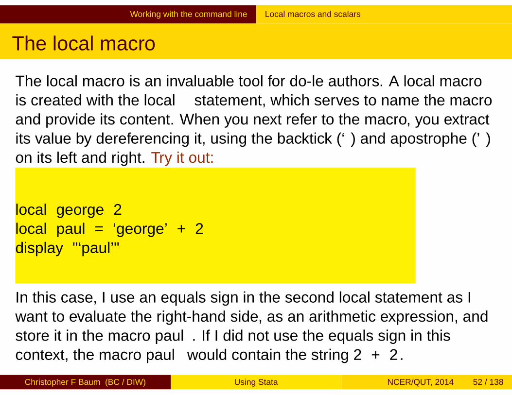
The local macro is an invaluable tool for do-file authors. A local macrois created with the local statement, which serves to name the macroand provide its content. When you next refer to the macro, you extractits value by dereferencing it, using the backtick (‘) and apostrophe (’)on its left and right. Try it out:
local george 2local paul = ‘george’ + 2display "‘paul’"
In this case, I use an equals sign in the second local statement as Iwant to evaluate the right-hand side, as an arithmetic expression, andstore it in the macro paul. If I did not use the equals sign in thiscontext, the macro paul would contain the string 2 + 2.
Christopher F Baum (BC / DIW) Using Stata NCER/QUT, 2014 52 / 138
Working with the command line forvalues and foreach
forvalues and foreach
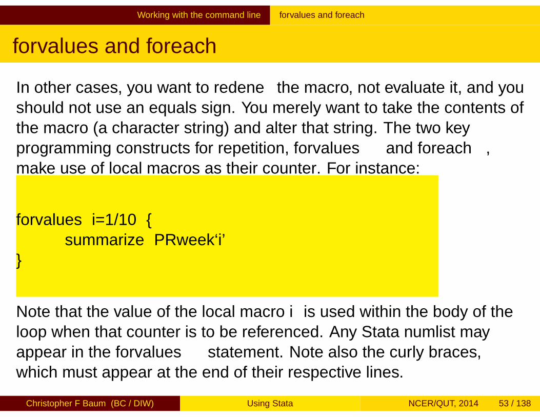
In other cases, you want to redefine the macro, not evaluate it, and youshould not use an equals sign. You merely want to take the contents ofthe macro (a character string) and alter that string. The two keyprogramming constructs for repetition, forvalues and foreach,make use of local macros as their “counter”. For instance:
forvalues i=1/10 {summarize PRweek‘i’
}
Note that the value of the local macro i is used within the body of theloop when that counter is to be referenced. Any Stata numlist mayappear in the forvalues statement. Note also the curly braces,which must appear at the end of their respective lines.
Christopher F Baum (BC / DIW) Using Stata NCER/QUT, 2014 53 / 138
Working with the command line forvalues and foreach
In many cases, the forvalues command will allow you to substituteexplicit statements with a single loop construct. By modifying the rangeand body of the loop, you can easily rewrite your do-file to handle adifferent case.
The foreach command is even more useful. It defines an iterationover any one of a number of lists:
the contents of a varlist (list of existing variables)the contents of a newlist (list of new variables)the contents of a numlist (list of integers)the separate words of a macrothe elements of an arbitrary list
Christopher F Baum (BC / DIW) Using Stata NCER/QUT, 2014 54 / 138
Working with the command line forvalues and foreach
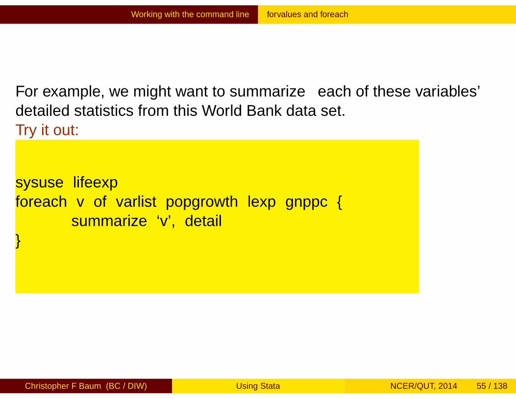
For example, we might want to summarize each of these variables’detailed statistics from this World Bank data set.Try it out:
sysuse lifeexpforeach v of varlist popgrowth lexp gnppc {
summarize ‘v’, detail}
Christopher F Baum (BC / DIW) Using Stata NCER/QUT, 2014 55 / 138
Working with the command line forvalues and foreach
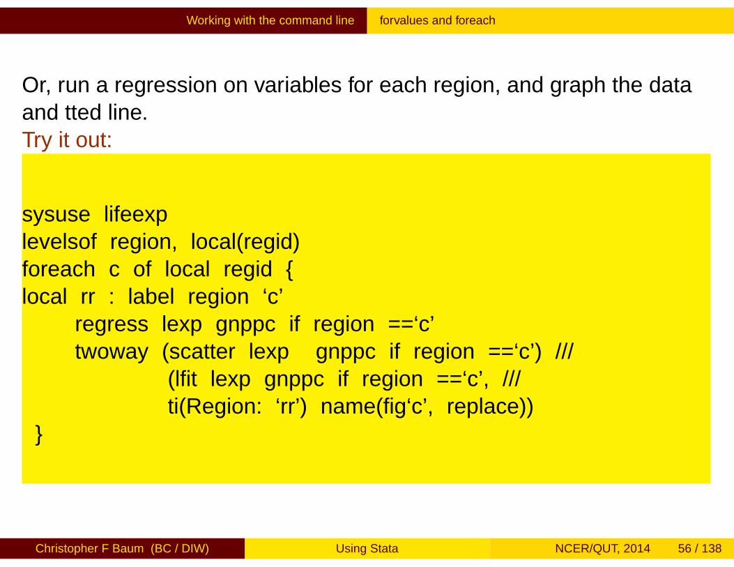
Or, run a regression on variables for each region, and graph the dataand fitted line.Try it out:
sysuse lifeexplevelsof region, local(regid)foreach c of local regid {local rr : label region ‘c’
regress lexp gnppc if region ==‘c’twoway (scatter lexp gnppc if region ==‘c’) ///
(lfit lexp gnppc if region ==‘c’, ///ti(Region: ‘rr’) name(fig‘c’, replace))
}
Christopher F Baum (BC / DIW) Using Stata NCER/QUT, 2014 56 / 138
Working with the command line forvalues and foreach
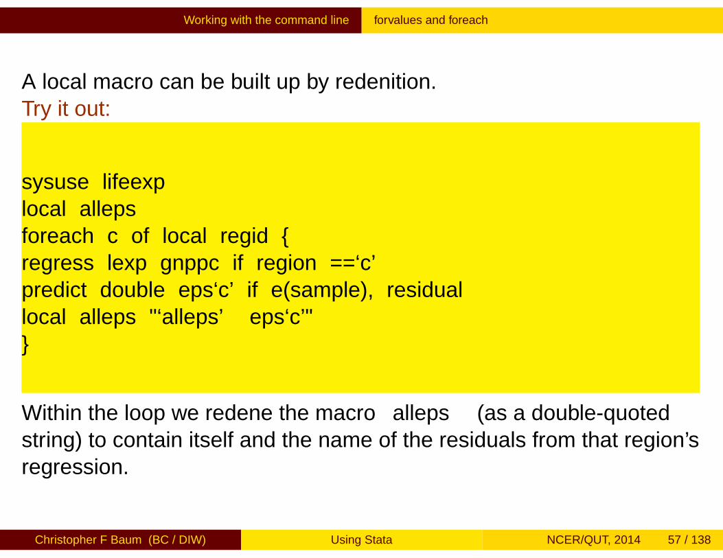
A local macro can be built up by redefinition.Try it out:
sysuse lifeexplocal allepsforeach c of local regid {regress lexp gnppc if region ==‘c’predict double eps‘c’ if e(sample), residuallocal alleps "‘alleps’ eps‘c’"}
Within the loop we redefine the macro alleps (as a double-quotedstring) to contain itself and the name of the residuals from that region’sregression.
Christopher F Baum (BC / DIW) Using Stata NCER/QUT, 2014 57 / 138
Working with the command line forvalues and foreach
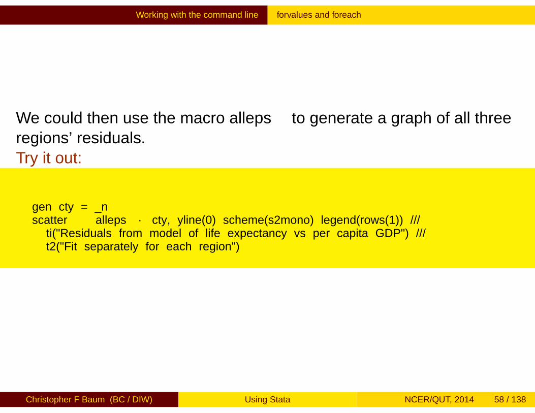
We could then use the macro alleps to generate a graph of all threeregions’ residuals.Try it out:
gen cty = _nscatter `alleps´ cty, yline(0) scheme(s2mono) legend(rows(1)) ///ti("Residuals from model of life expectancy vs per capita GDP") ///t2("Fit separately for each region")
Christopher F Baum (BC / DIW) Using Stata NCER/QUT, 2014 58 / 138

Working with the command line forvalues and foreach
-15
-10
-50
5
0 20 40 60 80cty
Eur & C.Asia N.A. S.A.
Fit separately for each regionResiduals from model of life expectancy vs per capita GDP
Christopher F Baum (BC / DIW) Using Stata NCER/QUT, 2014 59 / 138
Working with the command line forvalues and foreach
Global macros
Stata also supports global macros, which are referenced by a differentsyntax ($country rather than ‘country’). Global macros are usefulwhen particular definitions (e.g., the default working directory for aparticular project) are to be referenced in several do-files that are to beexecuted.
However, the creation of persistent objects of global scope can bedangerous, as global macro definitions are retained for the entire Statasession. One of the advantages of local macros is that they disappearwhen the do-file or ado-file in which they are defined finishesexecution.
Christopher F Baum (BC / DIW) Using Stata NCER/QUT, 2014 60 / 138
Working with the command line Prefix commands
Prefix commands
A number of Stata commands can be used as prefix commands,preceding a Stata command and modifying its behavior. The mostcommonly employed is the by prefix, which repeats a command over aset of categories. The statsby: prefix repeats the command, butcollects statistics from each category. The rolling: prefix runs thecommand on moving subsets of the data (usually time series).
Several other command prefixes: simulate:, which simulates astatistical model; bootstrap:, allowing the computation of bootstrapstatistics from resampled data; and jackknife:, which runs a commandover jackknife subsets of the data. The svy: prefix can be used withmany statistical commands to allow for survey sample design.
Christopher F Baum (BC / DIW) Using Stata NCER/QUT, 2014 61 / 138
Working with the command line The by prefix
The by prefix
You can often save time and effort by using the by prefix. When acommand is prefixed with a bylist, it is performed repeatedly for eachelement of the variable or variables in that list, each of which must becategorical.Try it out:
sysuse censusby region: summ pop medage
This one command provides descriptive statistics for each of four USCensus regions. If the data are not already sorted by the bylistvariables, the prefix bysort should be used. The option ,total willadd the overall summary.
Christopher F Baum (BC / DIW) Using Stata NCER/QUT, 2014 62 / 138
Working with the command line The by prefix
This can be extended to include more than one by-variable.Try it out:
sysuse censusgenerate large = (pop > 5000000) & !mi(pop)bysort region large: summ popurban death
This is a very handy tool, which often replaces explicit loops that mustbe used in other programs to achieve the same end.
The by-group logic will work properly even when some of the definedgroups have no observations. However, its limitation is that it can onlyexecute a single command for each category. If you want to estimate aregression for each group and save the residuals or predicted values,you must use an explicit loop.
Christopher F Baum (BC / DIW) Using Stata NCER/QUT, 2014 63 / 138
Working with the command line The by prefix
The by prefix should not be confused with the by option available onsome commands, which allows for specification of a grouping variable:for instance
ttest price, by(foreign)
will run a t-test for the difference of sample means across domesticand foreign cars.
Another useful aspect of by is the way in which it modifies themeanings of the observation number symbol. Usually _n refers to thecurrent observation number, which varies from 1 to _N, the maximumdefined observation. Under a bylist, _n refers to the observation withinthe bylist, and _N to the total number of observations for that category.This is often useful in creating new variables.
Christopher F Baum (BC / DIW) Using Stata NCER/QUT, 2014 64 / 138
Working with the command line The by prefix
For instance, if you have data on individuals with a family identifier,these commands might be useful:
sort famid ageby famid: generate famsize = _Nby famid: generate birthorder = _N - _n +1
Here the famsize variable is set to _N, the total number of records forthat family, while the birthorder variable is generated by sorting thefamily members’ ages within each family.
Christopher F Baum (BC / DIW) Using Stata NCER/QUT, 2014 65 / 138
Data management: principles of organization and transformation Missing values
Missing values
Missing value codes in Stata appear as the dot (.) in printed output(and a string missing value code as well: “”, the null string). It takes onthe largest possible positive value, so in the presence of missing datayou do not want to say
generate hiprice = (price > 10000) but rather
generate hiprice = (price > 10000) if price <. or
generate hiprice = (price > 10000) if !mi(price)
which then generates an indicator (dummy) variable equal to 1 forhigh-priced cars. The indicator will be zero for low-priced cars andmissing for cars with missing prices.
Christopher F Baum (BC / DIW) Using Stata NCER/QUT, 2014 66 / 138
Data management: principles of organization and transformation Missing values
Stata allows for multiple missing value codes (.a, .b, .c, ...,
.z). The standard missing value code (.) is the smallest amongthem, so testing for < . will always work. You may also use the missingfunction: mi(varname) will return 1 if the observation is a missingvalue, 0 otherwise.
Christopher F Baum (BC / DIW) Using Stata NCER/QUT, 2014 67 / 138

Data management: principles of organization and transformation Missing data handling
Missing data handling
An issue that often arises when importing data from external sourcesis the proper handling of missing data codes. Spreadsheet files oftenuse NA to denote missing values, while in some datasets codes suchas -9, -999, or -0.001 are used. The latter instances areparticularly worrisome as they may not be detected unless thevariables’ values are carefully scrutinized.
Note also that there is a missing value for string variables—the null, orzero-length string—which looks identical to a string of one or morespace characters.
Christopher F Baum (BC / DIW) Using Stata NCER/QUT, 2014 68 / 138
Data management: principles of organization and transformation Missing data handling
To properly handle missing values so that they are understood as suchin Stata, use the mvdecode command. This command allows you tomap various numeric values into numeric missing, or into one of theextended missing value codes .a, .b, ..., .z.
The mvencode command provides the inverse operation: particularlyuseful if you must transfer data to another package that uses someother convention for missing values.
Christopher F Baum (BC / DIW) Using Stata NCER/QUT, 2014 69 / 138

Data management: principles of organization and transformation Missing data handling
No matter what methods you have used to input external data to theStata workspace, you should immediately save the file in Stata formatand perform the describe and summarize commands. It is muchmore efficient to read a Stata-format .dta file with use than torepeatedly input a text file with any of the commands discussed above.If the file is large, you may want to use the compress command tooptimise Stata’s memory usage before saving it. compress isnon-destructive; it never reduces the stored precision of a variable.
Before any further use is made of this datafile, examine the results ofthe describe and summarize commands and ensure that eachvariable has been input properly, and that numeric variables havesensible values for their minima and maxima.
Christopher F Baum (BC / DIW) Using Stata NCER/QUT, 2014 70 / 138
Data management: principles of organization and transformation Display formats
Display formats
Each variable may have its own default display format. This does notalter the contents of the variable, but only affects how it is displayed.For instance, %9.2f would display a two-decimal-place real number.The command
format varname %9.2f
will save that format as the default format of the variable, and
format date %tm
will format a Stata date variable into a monthly format (e.g., 1998m10).
Christopher F Baum (BC / DIW) Using Stata NCER/QUT, 2014 71 / 138
Data management: principles of organization and transformation Variable labels
Variable labels
Each variable may have its own variable label. The variable label is acharacter string (maximum 80 characters) which describes thevariable, associated with the variable via
label variable varname "text"
Variable labels, where defined, will be used to identify the variable inprinted output, space permitting.
Christopher F Baum (BC / DIW) Using Stata NCER/QUT, 2014 72 / 138
Data management: principles of organization and transformation Value labels
Value labels
Value labels associate numeric values with character strings. Theyexist separately from variables, so that the same mapping of numericsto their definitions can be defined once and applied to a set ofvariables (e.g. 1=very satisfied...5=not satisfied may be applied to allresponses to questions about consumer satisfaction). Value labels aresaved in the dataset. For example:
label define sexlbl 0 male 1 femalelabel values sex sexlbl
The latter command associates the label sexlbl with the variablesex. Unlike other packages, Stata’s value labels are independent ofvariables, and the same label may be attached to any number ofvariables. If value labels are defined, they will be displayed in printedoutput instead of the numeric values.
Christopher F Baum (BC / DIW) Using Stata NCER/QUT, 2014 73 / 138
Data management: principles of organization and transformation Generating new variables
Generating new variables
The command generate is used to produce new variables in thedataset, whereas replace must be used to revise an existingvariable—and the command replace must always be spelled out.
A full set of functions are available for use in the generate command,including the standard mathematical functions, recode functions, stringfunctions, date and time functions, and specialized functions (helpfunctions for details). Note that generate’s sum() function is arunning or cumulative sum.
Christopher F Baum (BC / DIW) Using Stata NCER/QUT, 2014 74 / 138
Data management: principles of organization and transformation Generating new variables
As mentioned earlier, generate operates on all observations in thecurrent data set, producing a result or a missing value for each. Youneed not write explicit loops over the observations. You can, but it isusually bad programming practice to do so. You may restrictgenerate or replace to operate on a subset of the observationswith the if exp or in range qualifiers.
The if exp qualifier is usually more useful, but the in range qualifiermay be used to list a few observations of the data to examine theirvalidity. To list observations at the end of the current data set,use if -5/` to see the last five.
Christopher F Baum (BC / DIW) Using Stata NCER/QUT, 2014 75 / 138
Data management: principles of organization and transformation Generating new variables
You can take advantage of the fact that the exp specified in generatemay be a logical condition rather than a numeric or string value. Thisallows producing both the 0s and 1s of an indicator (dummy, orBoolean) variable in one command. For instance:
generate large = (pop > 5000000) & !mi(pop)
The condition & !mi(pop) makes use of two logical operators: &,AND, and !, NOT to add the qualifier that the result variable should bemissing if pop is missing, using the mi() function. Although numericfunctions of missing values are usually missing, creation of anindicator variable requires this additional step for safety.
The third logical operator is the Boolean OR, written as |. Note alsothat a test for equality is specified with the == operator (as in C). Thesingle = is used only for assignment.
Christopher F Baum (BC / DIW) Using Stata NCER/QUT, 2014 76 / 138
Data management: principles of organization and transformation Generating new variables
Keep in mind the important difference between the if exp qualifierand the if (or “programmer’s if”) command. Users of some alternativesoftware may be tempted to use a construct such as
generate raceid = .if (race == "Black")
replace raceid = 2
else if(race== "White")replace raceid = 3
which is perfectly valid syntactically. It is also useless, in that it willdefine the entire raceid variable based on the value of race of thefirst observation in the data set!
Christopher F Baum (BC / DIW) Using Stata NCER/QUT, 2014 77 / 138
Data management: principles of organization and transformation Generating new variables
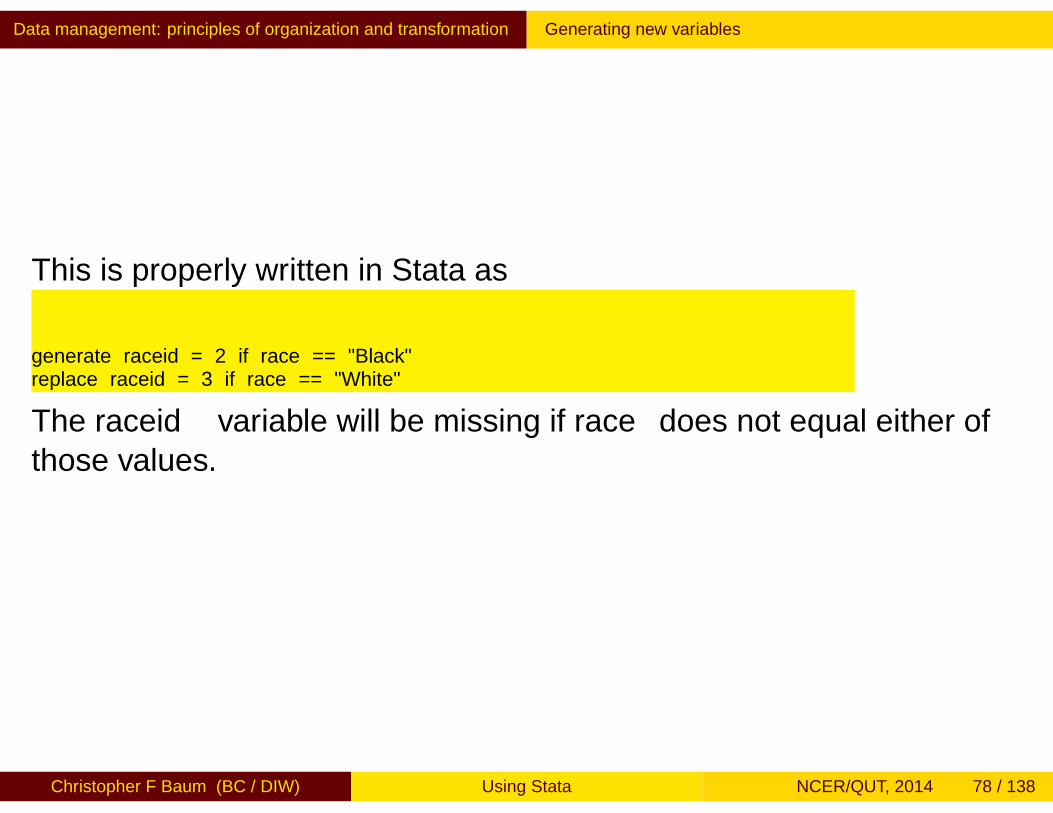
This is properly written in Stata as
generate raceid = 2 if race == "Black"replace raceid = 3 if race == "White"
The raceid variable will be missing if race does not equal either ofthose values.
Christopher F Baum (BC / DIW) Using Stata NCER/QUT, 2014 78 / 138
Data management: principles of organization and transformation Functions for generate, replace
Functions for generate and replace
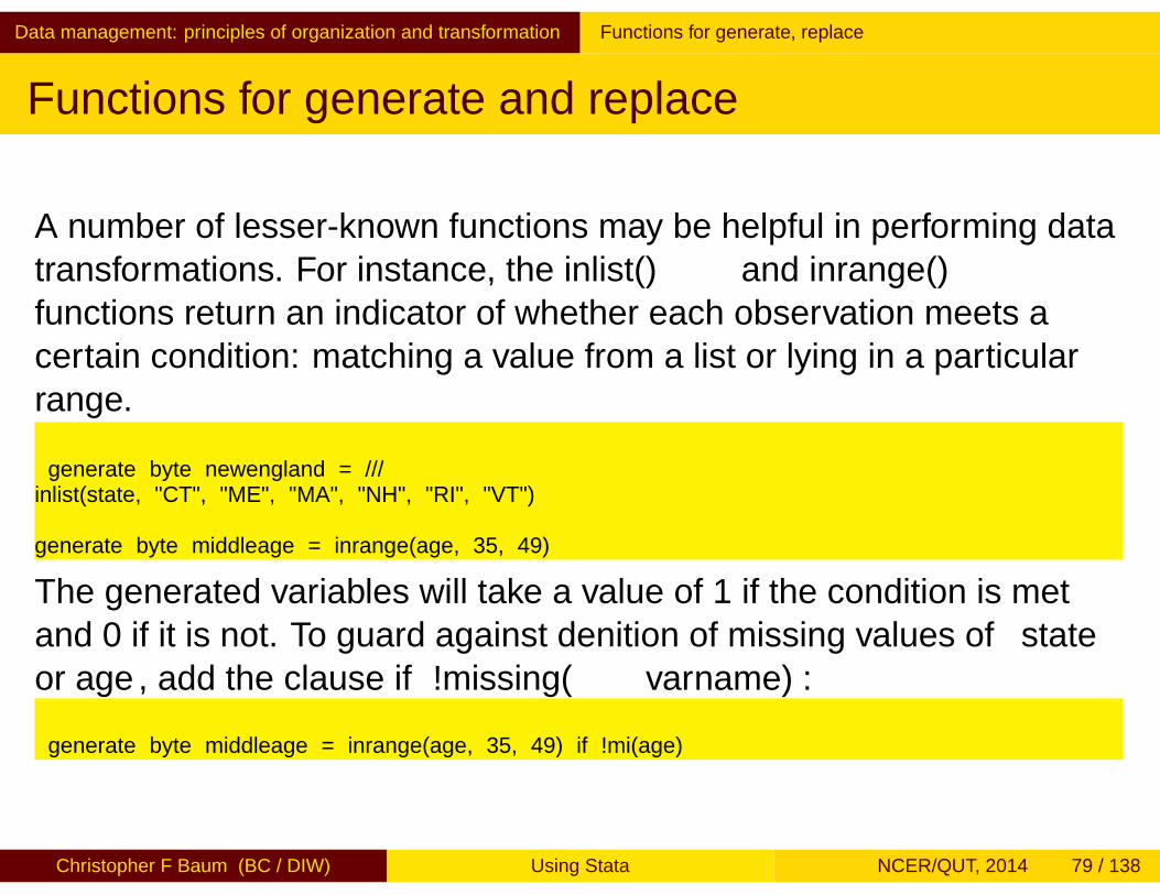
A number of lesser-known functions may be helpful in performing datatransformations. For instance, the inlist() and inrange()functions return an indicator of whether each observation meets acertain condition: matching a value from a list or lying in a particularrange.
generate byte newengland = ///inlist(state, "CT", "ME", "MA", "NH", "RI", "VT")
generate byte middleage = inrange(age, 35, 49)
The generated variables will take a value of 1 if the condition is metand 0 if it is not. To guard against definition of missing values of stateor age, add the clause if !missing(varname):
generate byte middleage = inrange(age, 35, 49) if !mi(age)
Christopher F Baum (BC / DIW) Using Stata NCER/QUT, 2014 79 / 138
Data management: principles of organization and transformation Functions for generate, replace
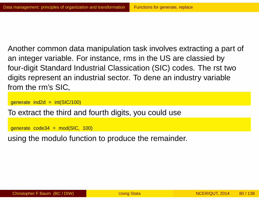
Another common data manipulation task involves extracting a part ofan integer variable. For instance, firms in the US are classified byfour-digit Standard Industrial Classification (SIC) codes. The first twodigits represent an industrial sector. To define an industry variablefrom the firm’s SIC,
generate ind2d = int(SIC/100)
To extract the third and fourth digits, you could use
generate code34 = mod(SIC, 100)
using the modulo function to produce the remainder.
Christopher F Baum (BC / DIW) Using Stata NCER/QUT, 2014 80 / 138

Data management: principles of organization and transformation Functions for generate, replace
The cond() function may often be used to avoid more complicatedcoding. It evaluates its first argument, and returns the secondargument if true, the third argument if false:
generate endqtr = cond( mod(month, 3) == 0, ///"Filing month", "Non-filing month")
Notice that in this example the endqtr variable need not be definedas string in the generate statement.
Christopher F Baum (BC / DIW) Using Stata NCER/QUT, 2014 81 / 138
Data management: principles of organization and transformation Functions for generate, replace
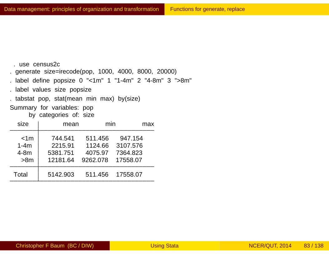
Stata contains both a recode command and a recode() function.These facilities may be used in lieu of a number of generate andreplace statements. There is also a irecode function to create anumeric code for values of a continuous variable falling in particularbrackets. For example, using a dataset containing population andmedian age for a number of US states:
Christopher F Baum (BC / DIW) Using Stata NCER/QUT, 2014 82 / 138
Data management: principles of organization and transformation Functions for generate, replace
. use census2c. generate size=irecode(pop, 1000, 4000, 8000, 20000)
. label define popsize 0 "<1m" 1 "1-4m" 2 "4-8m" 3 ">8m"
. label values size popsize
. tabstat pop, stat(mean min max) by(size)
Summary for variables: popby categories of: size
size mean min max
<1m 744.541 511.456 947.1541-4m 2215.91 1124.66 3107.5764-8m 5381.751 4075.97 7364.823>8m 12181.64 9262.078 17558.07
Total 5142.903 511.456 17558.07
Christopher F Baum (BC / DIW) Using Stata NCER/QUT, 2014 83 / 138
Data management: principles of organization and transformation Functions for generate, replace
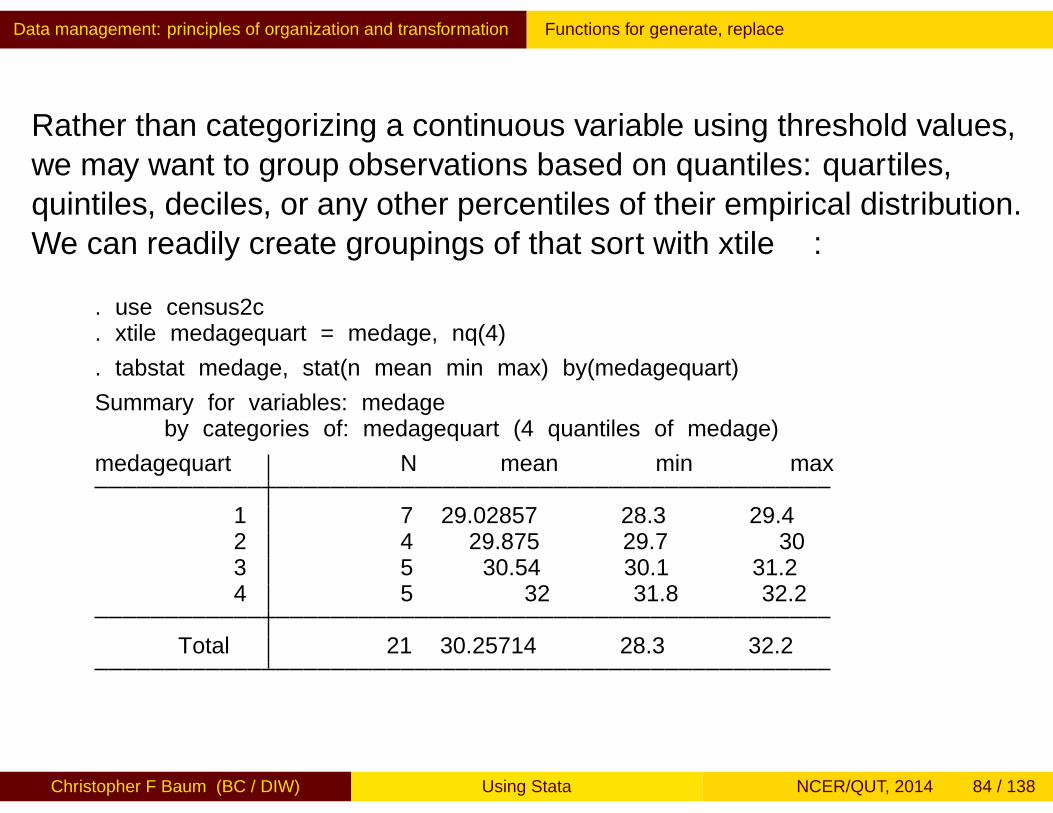
Rather than categorizing a continuous variable using threshold values,we may want to group observations based on quantiles: quartiles,quintiles, deciles, or any other percentiles of their empirical distribution.We can readily create groupings of that sort with xtile:
. use census2c
. xtile medagequart = medage, nq(4)
. tabstat medage, stat(n mean min max) by(medagequart)
Summary for variables: medageby categories of: medagequart (4 quantiles of medage)
medagequart N mean min max
1 7 29.02857 28.3 29.42 4 29.875 29.7 303 5 30.54 30.1 31.24 5 32 31.8 32.2
Total 21 30.25714 28.3 32.2
Christopher F Baum (BC / DIW) Using Stata NCER/QUT, 2014 84 / 138
Data management: principles of organization and transformation String-to-numeric conversion and vice versa
String-to-numeric conversion
A problem that commonly arises with data transferred fromspreadsheets is the automatic classification of a variable as stringrather than numeric. This often happens if the first value of such avariable is NA, denoting a missing value. If Stata’s convention fornumeric missings—the dot, or full stop (.) is used, this will not occur. Ifone or more variables are misclassified as string, how can they bemodified?
First, a warning. Do not try to maintain long numeric codes (such asUS Social Security numbers, with nine digits) in numeric form, as theywill generally be rounded off. Treat them as string variables, which maycontain up to 2,045 bytes.
Christopher F Baum (BC / DIW) Using Stata NCER/QUT, 2014 85 / 138
Data management: principles of organization and transformation String-to-numeric conversion and vice versa
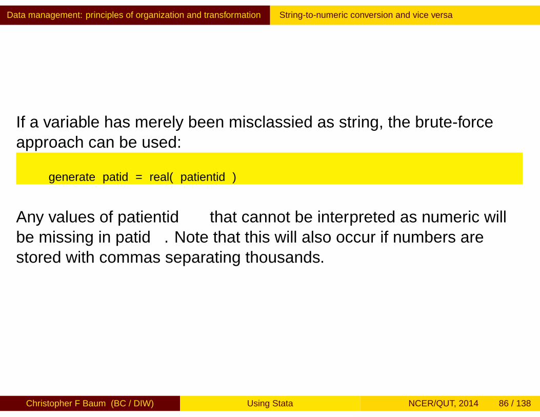
If a variable has merely been misclassified as string, the brute-forceapproach can be used:
generate patid = real( patientid )
Any values of patientid that cannot be interpreted as numeric willbe missing in patid. Note that this will also occur if numbers arestored with commas separating thousands.
Christopher F Baum (BC / DIW) Using Stata NCER/QUT, 2014 86 / 138

Data management: principles of organization and transformation String-to-numeric conversion and vice versa
A more subtle approach is given by the destring command, whichcan transform variables in place (with the replace option) and can beused with a varlist to apply the same transformation to a set ofvariables. Like the real() function, destring should only be usedon variables misclassified as strings.
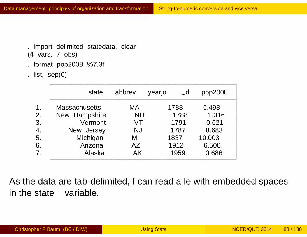
If the variable truly has string content and you need a numericequivalent, for statistical analysis, you may use encode on thevariable. To illustrate, let us read in some tab-delimited data withimport delimited.
Christopher F Baum (BC / DIW) Using Stata NCER/QUT, 2014 87 / 138
Data management: principles of organization and transformation String-to-numeric conversion and vice versa
. import delimited statedata, clear(4 vars, 7 obs)
. format pop2008 %7.3f
. list, sep(0)
state abbrev yearjo~d pop2008
1. Massachusetts MA 1788 6.4982. New Hampshire NH 1788 1.3163. Vermont VT 1791 0.6214. New Jersey NJ 1787 8.6835. Michigan MI 1837 10.0036. Arizona AZ 1912 6.5007. Alaska AK 1959 0.686
As the data are tab-delimited, I can read a file with embedded spacesin the state variable.
Christopher F Baum (BC / DIW) Using Stata NCER/QUT, 2014 88 / 138

Data management: principles of organization and transformation String-to-numeric conversion and vice versa
I want to create a categorical variable identifying each state with an(arbitrary) numeric code. This can be achieved with encode:
. encode state, gen(stid)
. list state stid, sep(0)
state stid
1. Massachusetts Massachusetts2. New Hampshire New Hampshire3. Vermont Vermont4. New Jersey New Jersey5. Michigan Michigan6. Arizona Arizona7. Alaska Alaska
. summarize stid
Variable Obs Mean Std. Dev. Min Max
stid 7 4 2.160247 1 7
Christopher F Baum (BC / DIW) Using Stata NCER/QUT, 2014 89 / 138

Data management: principles of organization and transformation String-to-numeric conversion and vice versa
Although stid is a numeric variable (as summarize shows) it isautomatically assigned a value label consisting of the contents ofstate. The variable stid may now be used in analyses requiringnumeric variables.
You may also want to make a variable into a string (for instance, toreinstate leading zeros in an id code variable). You may use thestring() function, the tostring command or the decodecommand to perform this operation.
Christopher F Baum (BC / DIW) Using Stata NCER/QUT, 2014 90 / 138
Data management: principles of organization and transformation The egen command
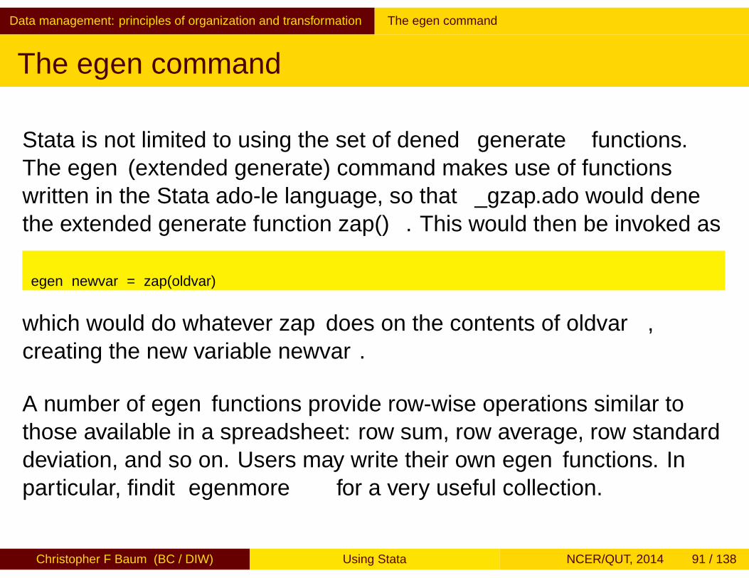
The egen command
Stata is not limited to using the set of defined generate functions.The egen (extended generate) command makes use of functionswritten in the Stata ado-file language, so that _gzap.ado would definethe extended generate function zap(). This would then be invoked as
egen newvar = zap(oldvar)
which would do whatever zap does on the contents of oldvar,creating the new variable newvar.
A number of egen functions provide row-wise operations similar tothose available in a spreadsheet: row sum, row average, row standarddeviation, and so on. Users may write their own egen functions. Inparticular, findit egenmore for a very useful collection.
Christopher F Baum (BC / DIW) Using Stata NCER/QUT, 2014 91 / 138
Data management: principles of organization and transformation The egen command
Although the syntax of an egen statement is very similar to that ofgenerate, several differences should be noted. As only a subset ofegen functions allow a by varlist: prefix or by(varlist) option, thedocumentation should be consulted to determine whether a particularfunction is byable, in Stata parlance. Similarly, the explicit use of _nand _N, often useful in generate and replace commands is notcompatible with egen.
Christopher F Baum (BC / DIW) Using Stata NCER/QUT, 2014 92 / 138
Data management: principles of organization and transformation The egen command
Wildcards may be used in row-wise functions. If you have state-levelU.S. Census variables pop1890, pop1900, ..., pop2000 youmay use egen nrCensus = rowmean(pop*) to compute theaverage population of each state over those decennial censuses. Therow-wise functions operate in the presence of missing values. Themean will be computed for all 50 states, although several were not partof the US in 1890.
Christopher F Baum (BC / DIW) Using Stata NCER/QUT, 2014 93 / 138
Data management: principles of organization and transformation The egen command
The number of non-missing elements in the row-wise varlist may becomputed with rownonmiss(), with rowmiss() as thecomplementary value. Other official row-wise functions includerowmax(), rowmin(), rowtotal() and rowsd() (row standarddeviation).
The functions rowfirst()and rowlast() give the first (last)non-missing values in the varlist. You may find this useful if thevariables refer to sequential items: for instance, wages earned peryear over several years, with missing values when unemployed.rowfirst() would return the earliest wage observation, androwlast() the most recent.
Christopher F Baum (BC / DIW) Using Stata NCER/QUT, 2014 94 / 138
Data management: principles of organization and transformation The egen command
Official egen also provides a number of statistical functions whichcompute a statistic for specified observations of a variable and placethat constant value in each observation of the new variable. Sincethese functions generally allow the use of by varlist:, they may beused to compute statistics for each by-group of the data. This facilitatescomputing statistics for each household for individual-level data oreach industry for firm-level data. The count(), mean(), min(),max() and total() functions are especially useful in this context.
As an illustration using our state-level data, we egen the averagepopulation in each of the size groups defined above, and expresseach state’s population as a percentage of the average population inthat size group. Size category 0 includes the smallest states in oursample.
Christopher F Baum (BC / DIW) Using Stata NCER/QUT, 2014 95 / 138
Data management: principles of organization and transformation The egen command
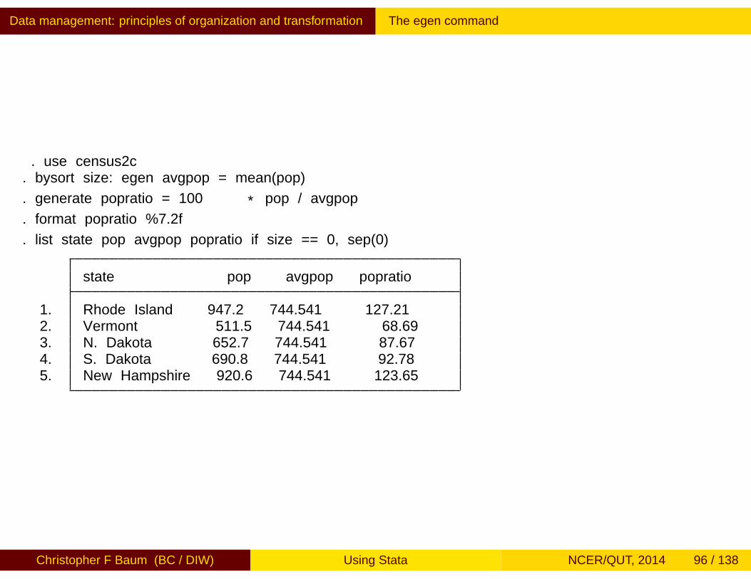
. use census2c. bysort size: egen avgpop = mean(pop)
. generate popratio = 100 * pop / avgpop
. format popratio %7.2f
. list state pop avgpop popratio if size == 0, sep(0)
state pop avgpop popratio
1. Rhode Island 947.2 744.541 127.212. Vermont 511.5 744.541 68.693. N. Dakota 652.7 744.541 87.674. S. Dakota 690.8 744.541 92.785. New Hampshire 920.6 744.541 123.65
Christopher F Baum (BC / DIW) Using Stata NCER/QUT, 2014 96 / 138
Data management: principles of organization and transformation The egen command
Other egen functions in this statistical category include iqr()(inter-quartile range), kurt() (kurtosis), mad() (median absolutedeviation), mdev() (mean absolute deviation), median(), mode(),pc() (percent or proportion of total), pctile(), p(n) (nth
percentile), rank(), sd() (standard deviation), skew() (skewness)and std() (z-score).
Many other egen functions are available; see help egen for details.
Christopher F Baum (BC / DIW) Using Stata NCER/QUT, 2014 97 / 138
Data management: principles of organization and transformation Time series calendar
Time series calendar
Stata supports date (and time) variables and the creation of a timeseries calendar variable. Dates are expressed, as they are in Excel, asthe number of days from a base date. In Stata’s case, that date is1 Jan 1960 (like Unix/Linux). You may set up data on an annual,half-yearly, quarterly, monthly, weekly or daily calendar, as well as acalendar that merely uses the observation number.
You may also set the delta of the calendar variable to be other than1: for instance, if you have data at five-year intervals, you may definethe data as annual with delta=5. This ensures that the lagged valueof the 2005 observation is that of 2000.
Christopher F Baum (BC / DIW) Using Stata NCER/QUT, 2014 98 / 138
Data management: principles of organization and transformation Time series calendar
A useful utility for setting the appropriate time series calendar istsmktim, available from the SSC Archive (ssc describetsmktim) and described in “Utility for time series data”, Baum, CF andWiggins, VL. Stata Technical Bulletin, 2000, 57, 2-4. It will set thecalendar, issuing the appropriate tsset command and the displayformat of the resulting calendar variable, and can be used in a paneldata context where each time series starts in the same calendarperiod.
Christopher F Baum (BC / DIW) Using Stata NCER/QUT, 2014 99 / 138
Data management: principles of organization and transformation Time series calendar
An observation-number calendar is generally necessary forbusiness-daily data where you want to avoid gaps for weekends,holidays etc. which will cause lagged values and differences to containmissing values. However, you may want to create two calendarvariables for the same time series data: one for statistical purposesand one for graphical purposes, which will allow the series to begraphed with calendar-date labels. This procedure is illustrated in“Stata Tip 40: Taking care of business...”, Baum, CF. Stata Journal,2007, 7:1, 137-139.
This is a moot point in Stata versions 12 and 13, which provide supportfor custom business-daily calendars (or bcals). As we shall see, Statacan construct the bcal from your dataset in version 13.
Christopher F Baum (BC / DIW) Using Stata NCER/QUT, 2014 100 / 138
Data management: principles of organization and transformation Time series operators
Time series operators
The D., L., and F. operators may be used under a time seriescalendar (including in the context of panel data) to specify firstdifferences, lags, and leads, respectively. These operators understandmissing data, and numlists: e.g. L(1/4).x is the first through fourthlags of x, while L2D.x is the second lag of the first difference of the xvariable.
Christopher F Baum (BC / DIW) Using Stata NCER/QUT, 2014 101 / 138
Data management: principles of organization and transformation Time series operators
It is very important to use the time series operators to refer to laggedor led values, rather than referring to the observation number (e.g.,_n-1). The time series operators respect the time series calendar, andwill not mistakenly compute a lag or difference from a prior period if itis missing. This is particularly important when working with panel datato ensure that references to one individual do not reach back into theprior individual’s data.
Christopher F Baum (BC / DIW) Using Stata NCER/QUT, 2014 102 / 138

Data management: principles of organization and transformation Time series operators
Using time series operators, you may not only consistently generatedifferences, lags, and leads, but may refer to them ‘on the fly’ instatistical and estimation commands. To estimate an AR(4) model, youneed not create the lagged variables.Try it out!
webuse lutkepohl, clearregress consumption L(1/4).consumption
To test Granger causality:
regress consumption L(-4/4).income
which would regress consumption on four leads, four lags and thecurrent value of income.
For a “Dickey–Fuller” style regression:
regress D.consumption L.consumption
Christopher F Baum (BC / DIW) Using Stata NCER/QUT, 2014 103 / 138
Reading external data import delimited
Reading external data with import delimited
Comma-separated (CSV) files or tab-delimited data files may be readvery easily with the import delimited command. If your file hasvariable names in the first row that are valid for Stata, they will beautomatically used (rather than default variable names). You usuallyneed not specify whether the data are tab- or comma-delimited. Notethat import delimited cannot read space-delimited data, norcharacter strings with embedded spaces, unless they aretab-delimited.
Christopher F Baum (BC / DIW) Using Stata NCER/QUT, 2014 104 / 138
Reading external data import delimited
The command presumes that the filetype is .csv:
import delimited using filename
You can also specify which rows and/or columns of the .csv file are tobe read.
Christopher F Baum (BC / DIW) Using Stata NCER/QUT, 2014 105 / 138
Reading external data import excel
Reading external data with import excel
In Stata 12 and 13, you may read data directly from Excel andExcel-compatible worksheets with the import excel command. Youmay specify from which sheet the data are to be loaded, and the rangeof that sheet in which they are located. You may also specify that thefirst row contains valid Stata variable names that are to be used. Forexample,
import excel using weo_201204_FR.xls, firstrow clear
Christopher F Baum (BC / DIW) Using Stata NCER/QUT, 2014 106 / 138
Reading external data import excel
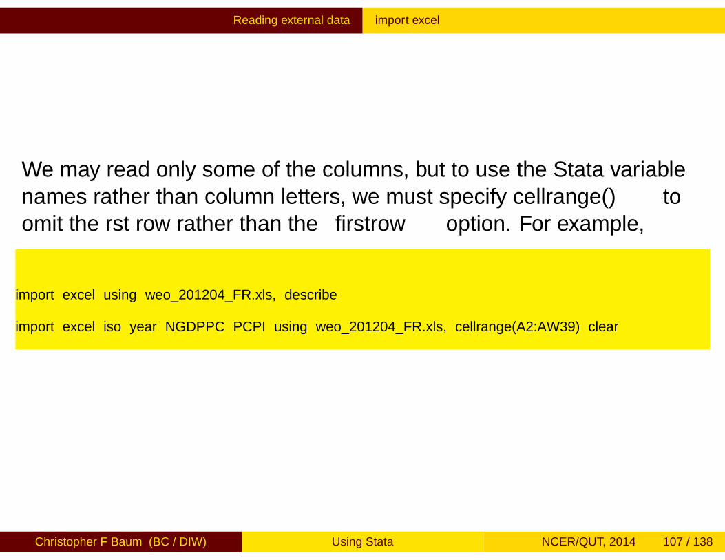
We may read only some of the columns, but to use the Stata variablenames rather than column letters, we must specify cellrange() toomit the first row rather than the firstrow option. For example,
import excel using weo_201204_FR.xls, describe
import excel iso year NGDPPC PCPI using weo_201204_FR.xls, cellrange(A2:AW39) clear
Christopher F Baum (BC / DIW) Using Stata NCER/QUT, 2014 107 / 138
Reading external data infile
Reading external data with infile
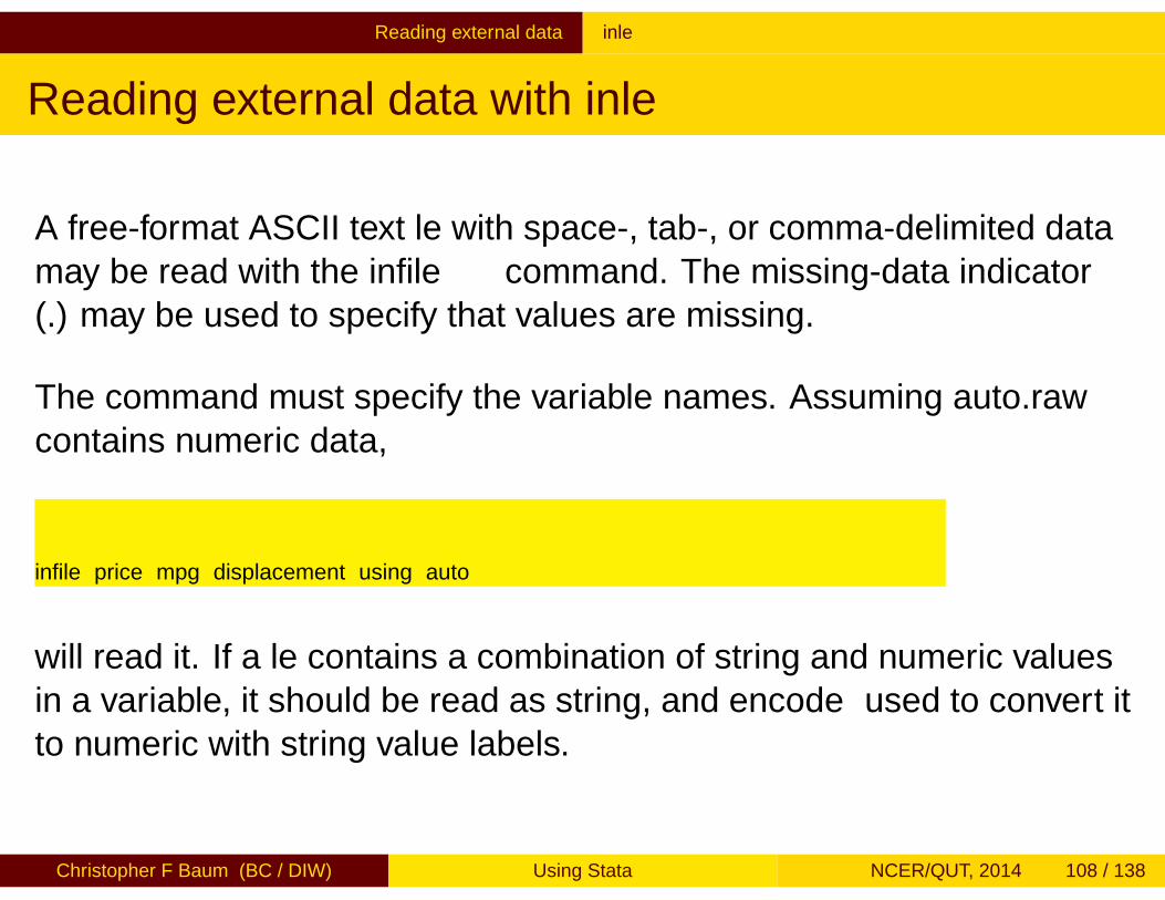
A free-format ASCII text file with space-, tab-, or comma-delimited datamay be read with the infile command. The missing-data indicator(.) may be used to specify that values are missing.
The command must specify the variable names. Assuming auto.rawcontains numeric data,
infile price mpg displacement using auto
will read it. If a file contains a combination of string and numeric valuesin a variable, it should be read as string, and encode used to convert itto numeric with string value labels.
Christopher F Baum (BC / DIW) Using Stata NCER/QUT, 2014 108 / 138
Reading external data infile
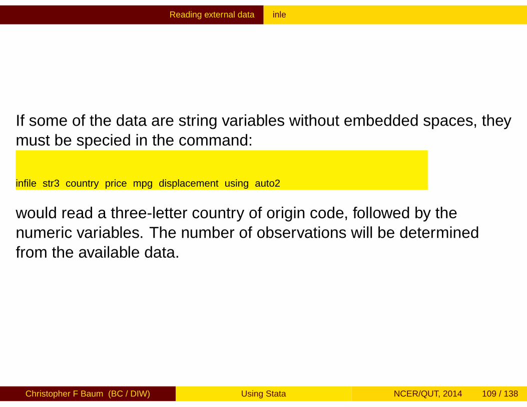
If some of the data are string variables without embedded spaces, theymust be specified in the command:
infile str3 country price mpg displacement using auto2
would read a three-letter country of origin code, followed by thenumeric variables. The number of observations will be determinedfrom the available data.
Christopher F Baum (BC / DIW) Using Stata NCER/QUT, 2014 109 / 138

Reading external data infile
The infile command may also be used with fixed-format data,including data containing undelimited string variables, by creating adictionary file which describes the format of each variable andspecifies where the data are to be found. The dictionary may alsospecify that more than one record in the input file corresponds to asingle observation in the data set.
Sometimes data fields are not delimited—for instance, the sequence‘102’ might actually represent three integer variables. A dictionarymust then be used to define the variables’ locations.
The byvariable() option allows a variable-wise dataset to be read,where one specifies the number of observations available for eachseries.
Christopher F Baum (BC / DIW) Using Stata NCER/QUT, 2014 110 / 138
Reading external data Stat/Transfer
Reading external data with Stat/Transfer
If your data are already in the internal format of SAS, SPSS, Excel,GAUSS, MATLAB, or a number of other packages, the best way to getit into Stata is by using the third-party product Stat/Transfer.
Stat/Transfer will preserve variable labels, value labels, and otheraspects of the data, and can be used to convert a Stata binary file intoother packages’ formats. It can also produce subsets of the data(selecting variables, cases or both) so as to generate an extract filethat is more manageable. This is particularly important when the2,047-variable limit on standard Stata data sets is encountered.
Christopher F Baum (BC / DIW) Using Stata NCER/QUT, 2014 111 / 138
Writing external data outfile
Writing external data: outfile
If you want to transfer data to another package, Stat/Transfer is veryuseful. But if you just want to create an ASCII file from Stata, theoutfile command may be used. It takes a varlist, and the if or inclauses may be used to control the observations to be exported.Applying sort prior to outfile will control the order of observations inthe external file. You may specify that the data are to be written incomma-separated format.
Christopher F Baum (BC / DIW) Using Stata NCER/QUT, 2014 112 / 138
Writing external data export delimited and file
Writing external data: export delimited and file
The export delimited command can write a comma-delimited ortab-delimited ASCII file, optionally placing the variable names in thefirst row. Such a file can be easily read by a spreadsheet programsuch as Excel.
For customized output, the file command can write out information(including scalars, matrices and macros, text strings, etc.) in any ASCIIor binary format of your choosing.
Christopher F Baum (BC / DIW) Using Stata NCER/QUT, 2014 113 / 138
Writing external data export excel
Writing external data: export excel
In Stata 12 and 13, the export excel command may be used towrite into a sheet of an Excel or Excel-compatible workbook. You maymodify or replace an existing sheet, and specify which Stata variablesare to be written to the worksheet. For example, after importing theFrench spreadsheet data:
export excel using myfrenchdata, firstrow(variables) replace
export excel iso year NGDPPC PCPI using myfrenchdata, replace
will create a new workbook, myfrenchdata.xls, containing allvariables in memory in the first example, and only the four specifiedvariables in the second example. You may also specify that Statavariable labels are to be output, rather than variable names.
Christopher F Baum (BC / DIW) Using Stata NCER/QUT, 2014 114 / 138
Writing external data postfile and post
Writing external data: postfile and post
A very useful capability is provided by the postfile and postcommands, which permit a Stata data set to be created in the courseof a program. For instance, you may be simulating the distribution of astatistic, fitting a model over separate samples, or bootstrappingstandard errors. Within the looping structure, you may post certainnumeric values to the postfile. This will create a separate Statabinary data set, which may then be opened in a later Stata run andanalyzed. Note that the parens () given in the documentation,surrounding each exp, are required.
Christopher F Baum (BC / DIW) Using Stata NCER/QUT, 2014 115 / 138
Combining data sets append
Combining data sets
In many empirical research projects, the raw data to be utilized arestored in a number of separate files: separate “waves” of panel data,timeseries data extracted from different databases, and the like. Stataonly permits a single data set to be accessed at one time. How, then,do you work with multiple data sets? Several commands are available,including append, merge, and joinby.
How, then, do you combine datasets in Stata? First of all, it isimportant to understand that at least one of the datasets to becombined must already have been saved in Stata format. Second, youshould realize that each of Stata’s commands for combining datasetsprovides a certain functionality, which should not confused with that ofother commands.
Christopher F Baum (BC / DIW) Using Stata NCER/QUT, 2014 116 / 138
Combining data sets append
The append command
The append command combines two Stata-format data sets thatpossess variables in common, adding observations to the existingvariables. The same variables need not be present in both files, aslong as a subset of the variables are common to the “master” and“using” data sets. It is important to note that “PRICE" and “price” aredifferent variables, and one will not be appended to the other.
Christopher F Baum (BC / DIW) Using Stata NCER/QUT, 2014 117 / 138
Combining data sets append
You might have a dataset on the demographic characteristics in 2007of the largest municipalities in China, cityCN. If you were given asecond dataset containing the same variables for the largestmunicipalities in Japan in 2007, cityJP, you might want to combinethose datasets with append. With the cityCN dataset in memory, youwould append using cityJP, which would add those records asadditional observations. You could then save the combined file under adifferent name. append can be used to combine multiple datasets, soif you had the additional files cityPH and cityMY, you could list thosefilenames in the using clause as well.
Prior to using append, it is a good idea to create an identifier variablein each dataset that takes on a constant value: e.g., gen country =1 in the CN dataset, gen country = 2 in the JP dataset, etc.
Christopher F Baum (BC / DIW) Using Stata NCER/QUT, 2014 118 / 138
Combining data sets append
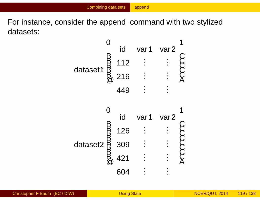
For instance, consider the append command with two stylizeddatasets:
dataset1 :
id var1 var2
112...
...
216...
...
449...
...
dataset2 :
id var1 var2
126...
...
309...
...
421...
...
604...
...
Christopher F Baum (BC / DIW) Using Stata NCER/QUT, 2014 119 / 138
Combining data sets append
These two datasets contain the same variables, as they must forappend to sensibly combine them. If dataset2 contained idcode,Var1, Var2 the two datasets could not sensibly be appended withoutrenaming the variables (recall that in Stata, var1 and Var1 are twoseparate variables). Appending these two datasets with commonvariable names creates a single dataset containing all of theobservations:
Christopher F Baum (BC / DIW) Using Stata NCER/QUT, 2014 120 / 138
Combining data sets append
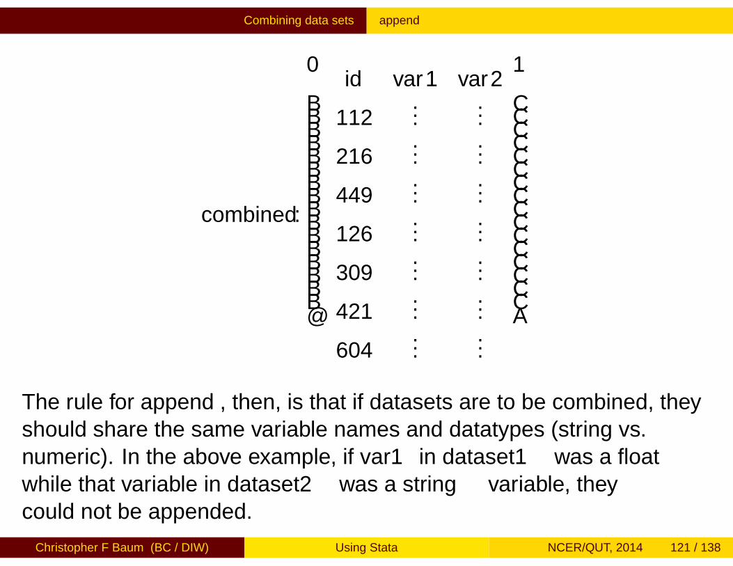
combined :
id var1 var2
112...
...
216...
...
449...
...
126...
...
309...
...
421...
...
604...
...
The rule for append, then, is that if datasets are to be combined, theyshould share the same variable names and datatypes (string vs.numeric). In the above example, if var1 in dataset1 was a floatwhile that variable in dataset2 was a string variable, theycould not be appended.
Christopher F Baum (BC / DIW) Using Stata NCER/QUT, 2014 121 / 138
Combining data sets append
It is permissible to append two datasets with differing variable names inthe sense that dataset2 could also contain an additional variable orvariables (for example, var3, var4). The values of those variables inthe observations coming from dataset1 would then be set to missing.
Some care must be taken when appending datasets in which the samevariable may exist with different data types (string in one, numeric inanother). For details, see “Stata tip 73: append with care!”, Baum CF,Stata Journal, 2008, 9:1, 166-168.
Christopher F Baum (BC / DIW) Using Stata NCER/QUT, 2014 122 / 138
Combining data sets merge
The merge command
We now describe the merge command, which is Stata’s basic tool forworking with more than one dataset. Its syntax changed considerablyin Stata version 11.
The merge command takes a first argument indicating whether you areperforming a one-to-one, many-to-one, one-to-many or many-to-manymerge using specified key variables. It can also perform a one-to-onemerge by observation.
Christopher F Baum (BC / DIW) Using Stata NCER/QUT, 2014 123 / 138
Combining data sets merge
Like the append command, the merge works on a “master”dataset—the current contents of memory—and a single “using”dataset (prior to Stata 11, you could specify multiple using datasets).One or more key variables are specified, and you need not sort eitherdataset prior to merging.
The distinction between “master” and “using” is important. When thesame variable is present in each of the files, Stata’s default behavior isto hold the master data inviolate and discard the using dataset’s copyof that variable. This may be modified by the update option, whichspecifies that non-missing values in the using dataset should replacemissing values in the master, and the even stronger updatereplace, which specifies that non-missing values in the using datasetshould take precedence.
Christopher F Baum (BC / DIW) Using Stata NCER/QUT, 2014 124 / 138
Combining data sets merge
A “one-to-one” merge (written merge 1:1) specifies that each recordin the using data set is to be combined with one record in the masterdata set. This would be appropriate if you acquired additional variablesfor the same observations.
In any use of merge, a new variable, _merge, takes on integer valuesindicating whether an observation appears in the master only, theusing only, or appears in both. This may be used to determine whetherthe merge has been successful, or to remove those observationswhich remain unmatched (e.g. merging a set of households fromdifferent cities with a comprehensive list of postal codes; one wouldthen discard all the unused postal code records). The _merge variablemust be dropped before another merge is performed on this data set.
Christopher F Baum (BC / DIW) Using Stata NCER/QUT, 2014 125 / 138
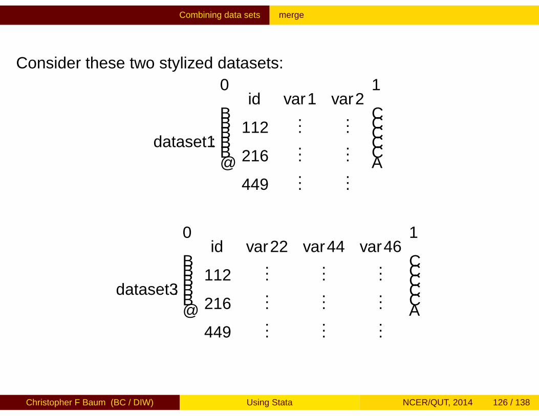
Combining data sets merge
Consider these two stylized datasets:
dataset1 :
id var1 var2
112...
...
216...
...
449...
...
dataset3 :
id var22 var44 var46
112...
......
216...
......
449...
......
Christopher F Baum (BC / DIW) Using Stata NCER/QUT, 2014 126 / 138
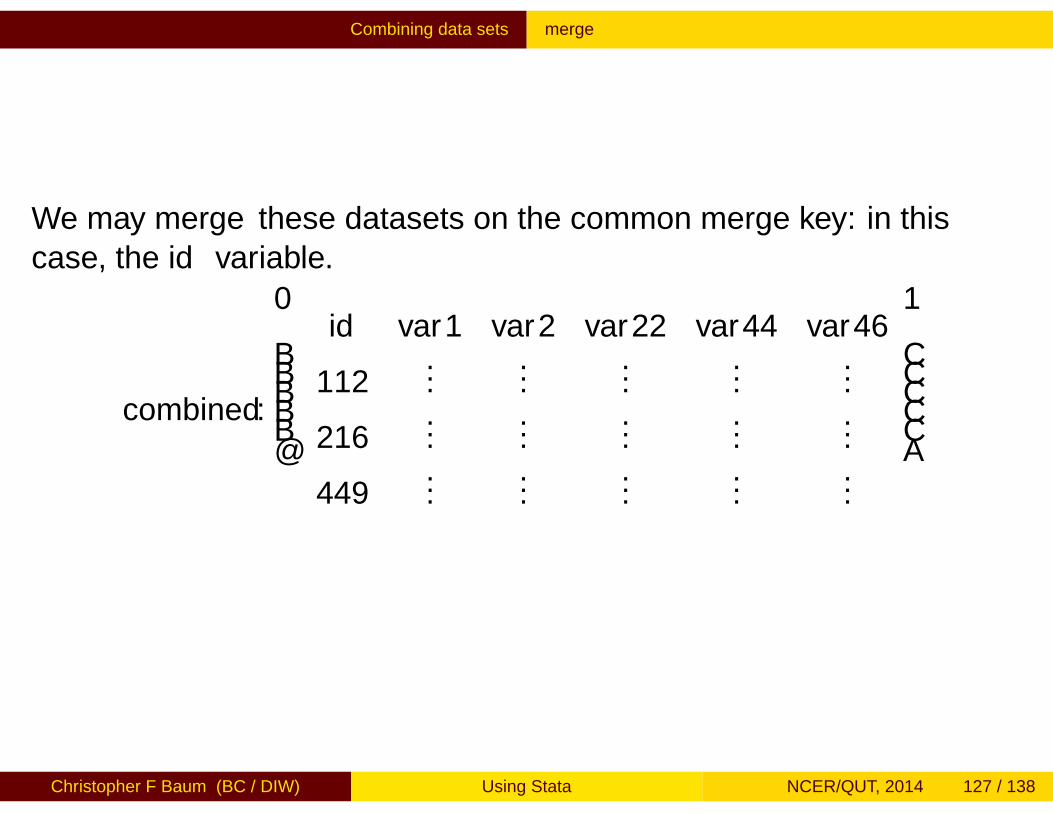
Combining data sets merge
We may merge these datasets on the common merge key: in thiscase, the id variable.
combined :
id var1 var2 var22 var44 var46
112...
......
......
216...
......
......
449...
......
......
Christopher F Baum (BC / DIW) Using Stata NCER/QUT, 2014 127 / 138
Combining data sets merge
The rule for merge, then, is that if datasets are to be combined on oneor more merge keys, they each must have one or more variables with acommon name and datatype (string vs. numeric). In the exampleabove, each dataset must have a variable named id. That variable canbe numeric or string, but that characteristic of the merge key variablesmust match across the datasets to be merged. Of course, we need nothave exactly the same observations in each dataset: if dataset3contained observations with additional id values, those observationswould be merged with missing values for var1 and var2.
This is the simplest kind of merge: the one-to-one merge. Statasupports several other types of merges. But the key concept should beclear: the merge command combines datasets “horizontally”, addingvariables’ values to existing observations.
Christopher F Baum (BC / DIW) Using Stata NCER/QUT, 2014 128 / 138
Combining data sets Match merge
The merge command can also do a “many-to-one"’ or “one-to-many”merge. For instance, you might have a dataset named hospitalsand a dataset named discharges, both of which contain a hospitalID variable hospid. If you had the hospitals dataset in memory,you could merge 1:m hospid using discharges to match eachhospital with its prior patients. If you had the discharges dataset inmemory, you could merge m:1 hospid using hospitals to addthe hospital characteristics to each discharge record. This is a veryuseful technique to combine aggregate data with disaggregate datawithout dealing with the details.
Although “many-to-one"’ or “one-to-many” merges are commonplaceand very useful, you should never want to do a “many-to-many” (m:m)merge, which will yield seemingly random results.
Christopher F Baum (BC / DIW) Using Stata NCER/QUT, 2014 129 / 138
Combining data sets Match merge
The long-form dataset is very useful if you want to add aggregate-levelinformation to individual records. For instance, we may have paneldata for a number of companies for several years. We may want toattach various macro indicators (interest rate, GDP growth rate, etc.)that vary by year but not by company. We would place those macrovariables into a dataset, indexed by year, and sort it by year.
We could then use the firm-level panel dataset and sort it by year. Amerge command can then add the appropriate macro variables toeach instance of year. This use of merge is known as a one-to-manymatch merge, where the year variable is the merge key.
Note that the merge key may contain several variables: we might haveinformation specific to industry and year that should be merged ontoeach firm’s observations.
Christopher F Baum (BC / DIW) Using Stata NCER/QUT, 2014 130 / 138
Reconfiguring data sets
Reconfiguring data sets
Data are often provided in a different orientation than that required forstatistical analysis. The most common example of this occurs withpanel, or longitudinal, data, in which each observation conceptuallyhas both cross-section (i) and time-series (t) subscripts. Often one willwant to work with a “pure” cross-section or “pure” time-series. If themicrodata themselves are the objects of analysis, this can be handledwith sorting and a loop structure. If you have data for N firms for Tperiods per firm, and want to fit the same model to each firm, onecould use the statsby command, or if more complex processing ofeach model’s results was required, a foreach block could be used. Ifanalysis of a cross-section was desired, a bysort would do the job.
Christopher F Baum (BC / DIW) Using Stata NCER/QUT, 2014 131 / 138

Reconfiguring data sets collapse
But what if you want to use average values for each time period,averaged over firms? The resulting dataset of T observations can beeasily created by the collapse command, which permits you togenerate a new data set comprised of summary statistics of specifiedvariables. More than one summary statistic can be generated per inputvariable, so that both the number of firms per period and the averagereturn on assets could be generated. collapse can produce counts,means, medians, percentiles, extrema, and standard deviations.
Christopher F Baum (BC / DIW) Using Stata NCER/QUT, 2014 132 / 138
Reconfiguring data sets reshape
reshape
Different models applied to longitudinal data require differentorientations of those data. For instance, seemingly unrelatedregressions (sureg) require the data to have T observations (“wide”),with separate variables for each cross–sectional unit. Fixed–effects orrandom-effects regression models xtreg, on the other hand, requirethat the data be stacked or “vec”’d in the “long” format. It is usuallymuch easier to generate transformations of the data in stacked format,where a single variable is involved.
The reshape command allows you to transfer the data from theformer (“wide”) format to the latter (“long”) format or vice versa. It is acomplicated command, because of the many variations on thisprocess one might encounter, but it is very powerful.
Christopher F Baum (BC / DIW) Using Stata NCER/QUT, 2014 133 / 138
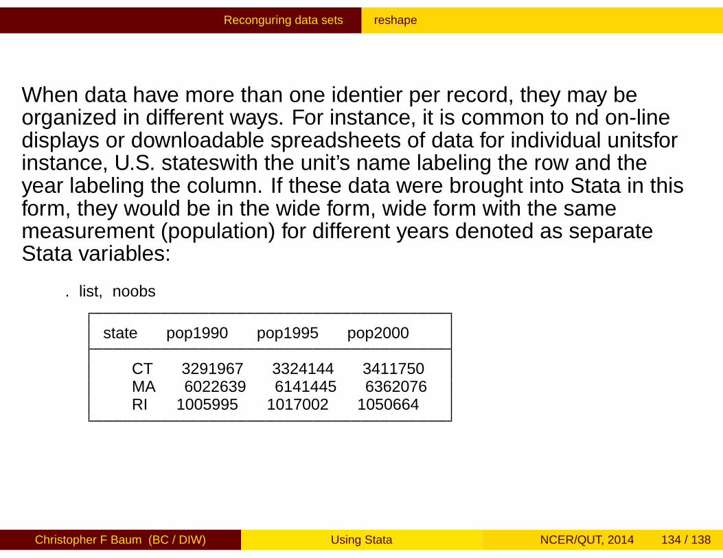
Reconfiguring data sets reshape
When data have more than one identifier per record, they may beorganized in different ways. For instance, it is common to find on-linedisplays or downloadable spreadsheets of data for individual units—forinstance, U.S. states—with the unit’s name labeling the row and theyear labeling the column. If these data were brought into Stata in thisform, they would be in the wide form, wide form with the samemeasurement (population) for different years denoted as separateStata variables:
. list, noobs
state pop1990 pop1995 pop2000
CT 3291967 3324144 3411750MA 6022639 6141445 6362076RI 1005995 1017002 1050664
Christopher F Baum (BC / DIW) Using Stata NCER/QUT, 2014 134 / 138

Reconfiguring data sets reshape
There are a number of Stata commands—such as egen row-wisefunctions—which work effectively on data stored in the wide form. Itmay also be a useful form of data organization for producing graphs.
Alternatively, we can imagine stacking each year’s population figuresfrom this display into one variable, pop. In this format, known in Stataas the long form, each datum is identified by two variables: the statename and the year to which it pertains.
Christopher F Baum (BC / DIW) Using Stata NCER/QUT, 2014 135 / 138
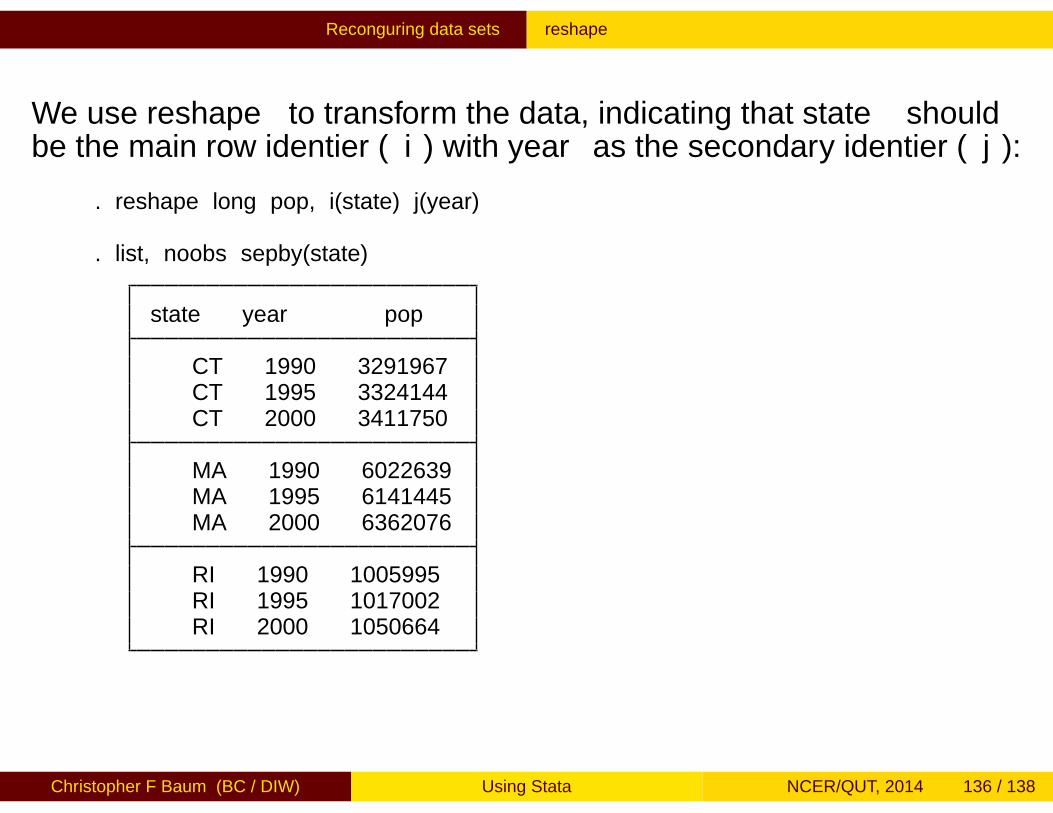
Reconfiguring data sets reshape
We use reshape to transform the data, indicating that state shouldbe the main row identifier (i) with year as the secondary identifier (j):
. reshape long pop, i(state) j(year)
. list, noobs sepby(state)
state year pop
CT 1990 3291967CT 1995 3324144CT 2000 3411750
MA 1990 6022639MA 1995 6141445MA 2000 6362076
RI 1990 1005995RI 1995 1017002RI 2000 1050664
Christopher F Baum (BC / DIW) Using Stata NCER/QUT, 2014 136 / 138
Reconfiguring data sets reshape
This data structure is required for many of Stata’s statisticalcommands, such as the xt suite of panel data commands. The longform is also very useful for data management using by-groups and thecomputation of statistics at the individual level, often implemented withthe collapse command.
Inevitably, you will acquire data (either raw data or Stata datasets) thatare stored in either the wide or the long form and will find thattranslation to the other format is necessary to carry out your analysis.In statistical packages lacking a data-reshape feature, commonpractice entails writing the data to one or more external text files andreading it back in.
Christopher F Baum (BC / DIW) Using Stata NCER/QUT, 2014 137 / 138
Reconfiguring data sets reshape
With the proper use of reshape, writing data out and reading themback in is not necessary in Stata. But reshape requires, first of all,that the data to be reshaped are labelled in such a way that they canbe handled by the mechanical rules that the command applies. Insituations beyond the simple application of reshape, it may requiresome experimentation to construct the appropriate command syntax.This is all the more reason for enshrining that code in a do-file as someday you are likely to come upon a similar application for reshape.
An illustration of advanced use of reshape on data from InternationalFinancial Statistics is provided in Baum CF, Cox NJ, “Stata tip 45:Getting those data into shape,” Stata Journal, 2007, 7, 268–271.
Christopher F Baum (BC / DIW) Using Stata NCER/QUT, 2014 138 / 138


![E B DAVID AUBERT E LA VENGANCE DE LA MORT … · Judas qui le vendi ... soltanto la biografia leggendaria di Giuda era stata pubblicata da ... dell’apostolo [Baum 1916: 536-41].](https://static.fdocuments.in/doc/165x107/5bb5e22109d3f250788dacd7/e-b-david-aubert-e-la-vengance-de-la-mort-judas-qui-le-vendi-soltanto-la.jpg)