Christopher F Baum - Boston Collegefm · Christopher F Baum (BC / DIW) Count & Categorical Data...

Models for Count Dataand Categorical Response Data

Christopher F Baum

Boston College and DIW Berlin

June 2010

Christopher F Baum (BC / DIW) Count & Categorical Data June 2010 1 / 66

Poisson and negative binomial regression

Poisson regression

In statistical analyses, dependent variables may be limited by beingcount data, only taking on nonnegative (or only positive) integervalues. This is a natural form for data such as the number of childrenper family, the number of jobs an individual has held or the number ofcountries in which a company operates manufacturing facilities.

Just as with the other limited dependent variable models we havediscussed, linear regression is not an appropriate estimation techniquefor count data, as it fails to take into account the limited number ofpossible values of the response variable.


Poisson and negative binomial regression Poisson regression

The most common technique employed to model count data is Poissonregression, so named because the error process is assumed to followthe Poisson distribution. As an aside, you may notice that the insignia(colophon) of Stata Press appears to be a soldier with a horse. ThePoisson distribution was first applied to data on the number ofPrussian cavalrymen who died after being kicked by a horse, and thecolophon refers to that historical detail.



The technique is implemented in Stata by the poisson command,which has the same format as other estimation commands, where thedepvar is a nonnegative count variable; that is, it may be zero. It is amaximum likelihood estimation technique.

In some contexts, the Poisson distribution describes the number ofevents that occur in a given time period where its mean µ is theaverage number of events per period. It has the unusual feature that itsmean equals its variance. Its probability density function isPr(Y = y) =

(e−µµy

y!

), y=0,1,2,. . . where e is the base of the natural

logarithms and y ! is the factorial of y .

The skewness of the Poisson distribution is (1/√µ) and the kurtosis is

(3 + 1/µ), so that for large µ, the distribution approaches the NormalN(µ, µ) with skewness of zero and kurtosis of three.



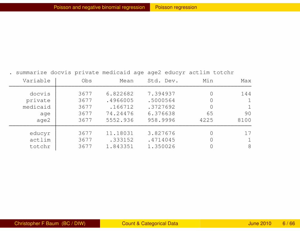
We illustrate count data techniques using a dataset from the U.S.Medical Expenditure Panel Survey (MEPS) containing information onthe number of doctor visits in 2003 (docvis) for a number of elderlypatients as well as a number of patient characteristics.

private is an indicator of private insurance coverage, supplementalto Medicare. medicaid indicates the patient is eligible for low-incomeMedicaid coverage. actlim indicates the presence of activitylimitations, while totchr is the number of chronic conditions. educyrindicates the number of years of education attained.



. summarize docvis private medicaid age age2 educyr actlim totchr

Variable Obs Mean Std. Dev. Min Max

docvis 3677 6.822682 7.394937 0 144private 3677 .4966005 .5000564 0 1

medicaid 3677 .166712 .3727692 0 1age 3677 74.24476 6.376638 65 90age2 3677 5552.936 958.9996 4225 8100

educyr 3677 11.18031 3.827676 0 17actlim 3677 .333152 .4714045 0 1totchr 3677 1.843351 1.350026 0 8



The default parameterization of the Poisson model, in which theconditional mean of observation i depends on a number of covariates,is the exponential mean:

µi = exp(x ′i β), i = 1, ...,N

This model may be estimated by maximum likelihood (ML), where theparameter estimates are the solutions to the first order conditions

N∑i=1

(yi − exp(x ′i β))xi = 0

The likelihood function is globally concave and the estimationconverges rapidly.



. poisson docvis private medicaid age age2 educyr actlim totchr, nolog

Poisson regression Number of obs = 3677LR chi2(7) = 4477.98Prob > chi2 = 0.0000

Log likelihood = -15019.64 Pseudo R2 = 0.1297

docvis Coef. Std. Err. z P>|z| [95% Conf. Interval]

private .1422324 .0143311 9.92 0.000 .114144 .1703208medicaid .0970005 .0189307 5.12 0.000 .0598969 .134104

age .2936722 .0259563 11.31 0.000 .2427988 .3445457age2 -.0019311 .0001724 -11.20 0.000 -.0022691 -.0015931

educyr .0295562 .001882 15.70 0.000 .0258676 .0332449actlim .1864213 .014566 12.80 0.000 .1578726 .2149701totchr .2483898 .0046447 53.48 0.000 .2392864 .2574933_cons -10.18221 .9720115 -10.48 0.000 -12.08732 -8.277101



If the model is correctly specified, but the distribution of errors is notPoisson (as we will discuss next) one approach is to estimate themodel with pseudo-ML, generating robust standard errors:

. poisson docvis private medicaid age age2 educyr actlim totchr, ///> vce(robust) nolog

Poisson regression Number of obs = 3677Wald chi2(7) = 720.43Prob > chi2 = 0.0000

Log pseudolikelihood = -15019.64 Pseudo R2 = 0.1297

Robustdocvis Coef. Std. Err. z P>|z| [95% Conf. Interval]

private .1422324 .036356 3.91 0.000 .070976 .2134889medicaid .0970005 .0568264 1.71 0.088 -.0143773 .2083783

age .2936722 .0629776 4.66 0.000 .1702383 .4171061age2 -.0019311 .0004166 -4.64 0.000 -.0027475 -.0011147

educyr .0295562 .0048454 6.10 0.000 .0200594 .039053actlim .1864213 .0396569 4.70 0.000 .1086953 .2641474totchr .2483898 .0125786 19.75 0.000 .2237361 .2730435_cons -10.18221 2.369212 -4.30 0.000 -14.82578 -5.538638



Although all parameters (except medicaid) are still highly significant,the standard errors and z-statistics are much smaller, indicating thatthe errors may not be distributed as Poisson.

The coefficients may be interpreted as semielasticities. A coefficient of0.029 on educyr indicates that a patient with one more year ofeducation is expected to have 2.9% more doctor visits.



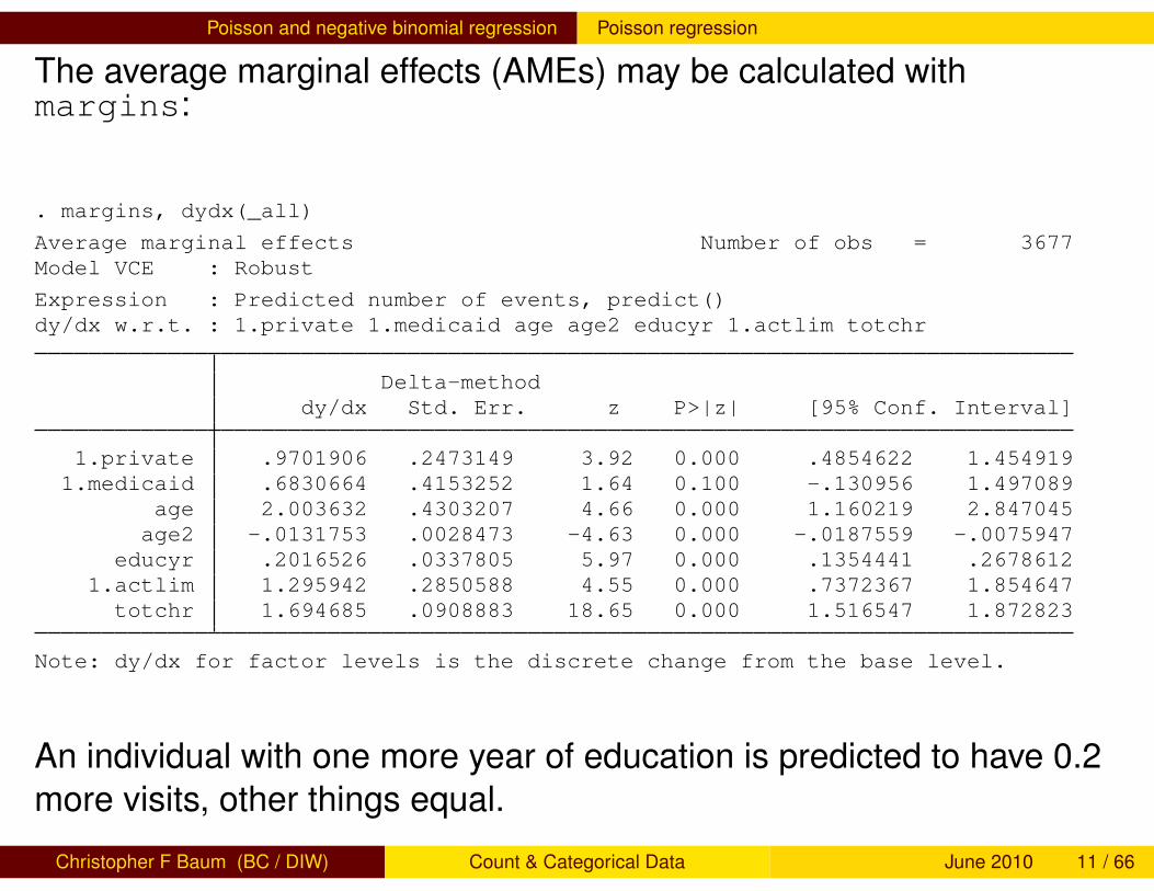
The average marginal effects (AMEs) may be calculated withmargins:

. margins, dydx(_all)

Average marginal effects Number of obs = 3677Model VCE : Robust

Expression : Predicted number of events, predict()dy/dx w.r.t. : 1.private 1.medicaid age age2 educyr 1.actlim totchr

Delta-methoddy/dx Std. Err. z P>|z| [95% Conf. Interval]

1.private .9701906 .2473149 3.92 0.000 .4854622 1.4549191.medicaid .6830664 .4153252 1.64 0.100 -.130956 1.497089

age 2.003632 .4303207 4.66 0.000 1.160219 2.847045age2 -.0131753 .0028473 -4.63 0.000 -.0187559 -.0075947

educyr .2016526 .0337805 5.97 0.000 .1354441 .26786121.actlim 1.295942 .2850588 4.55 0.000 .7372367 1.854647

totchr 1.694685 .0908883 18.65 0.000 1.516547 1.872823

Note: dy/dx for factor levels is the discrete change from the base level.

An individual with one more year of education is predicted to have 0.2more visits, other things equal.


Poisson and negative binomial regression Negative binomial regression

Negative binomial regression

A limitation of the Poisson distribution is the equality of its mean andvariance. We may often observe count data processes where thisequality is not reasonable: in particular, where the conditional varianceis larger than the conditional mean. This is termed overdispersion, andits presence renders the assumption of a Poisson distribution for theerror process untenable. It is particularly likely to occur in the case ofunobserved heterogeneity.

In this circumstance, a reasonable alternative is negative binomialregression. This model allows the variance to differ from the mean. Inits Stata implementation as nbreg, a Poisson model is also estimatedand a test of overdispersion is provided. If the dispersion parameter iszero, it is appropriate to fit a Poisson regression model.



The negative binomial (NB) distribution is a two-parameter distribution.For positive integer n, it is the distribution of the number of failures thatoccur in a sequence of trials before n successes have occurred, wherethe probability of success in each trial is p. The distribution is definedfor any positive n. The negative binomial distribution is a mixture of thePoisson distribution and the Gamma distribution, or generalizedfactorial function.

Unlike the Poisson, which is fully characterized by its mean µ, the NBdistribution is a function of both µ and α. Its mean is still µ, but itsconditional variance is µ(1 + αµ). As is evident, as α→ 0, thedistribution becomes the Poisson distribution.



We reestimate the model with Stata’s nbreg:

. nbreg docvis private medicaid age age2 educyr actlim totchr, nolog

Negative binomial regression Number of obs = 3677LR chi2(7) = 773.44

Dispersion = mean Prob > chi2 = 0.0000Log likelihood = -10589.339 Pseudo R2 = 0.0352

docvis Coef. Std. Err. z P>|z| [95% Conf. Interval]

private .1640928 .0332186 4.94 0.000 .0989856 .2292001medicaid .100337 .0454209 2.21 0.027 .0113137 .1893603

age .2941294 .0601588 4.89 0.000 .1762203 .4120384age2 -.0019282 .0004004 -4.82 0.000 -.0027129 -.0011434

educyr .0286947 .0042241 6.79 0.000 .0204157 .0369737actlim .1895376 .0347601 5.45 0.000 .121409 .2576662totchr .2776441 .0121463 22.86 0.000 .2538378 .3014505_cons -10.29749 2.247436 -4.58 0.000 -14.70238 -5.892595

/lnalpha -.4452773 .0306758 -.5054007 -.3851539

alpha .6406466 .0196523 .6032638 .6803459

Likelihood-ratio test of alpha=0: chibar2(01) = 8860.60 Prob>=chibar2 = 0.000



The likelihood ratio test of α = 0 strongly rejects the null hypothesisthat the errors do not exhibit overdispersion. Thus, the Poissonregression model is rejected in favor of its generalized version, the NBregression model. The coefficients are similar between the twomodels, and the NB estimates are comparable to those from poissonwith robust standard errors.


Extended count data models

Extended count data models

In many social science datasets, count data may include a largenumber of zero values. If the data were dichotomized into zero andnon-zero subsets so that a probit or logit model could be fit, theunconditional probability of zero would be sizable: larger than thatarising in a Poisson or negative binomial distribution. For instance, wemight have a random sample from the population in which the numberof postgraduate degrees is recorded. For many individuals, the countwill be zero. For many professionals, it will be one, and for mostacademics, it will be two (or more).


Extended count data models zero-inflated models

To model data with these characteristics, we may employ thezero-inflated variants of Poisson regression (zip) or negative binomialregression (zinb). In these commands, there is an auxiliary logitmodel specified in the inflate()) option that determines whetherthe observed count is zero. This model could contain only a constantor additional covariates.

With the vuong option, a test of the ZIP versus standard Poissonregression model is computed. For zinb, the zip option computes atest of the zinb model versus the zero-inflated Poisson model which isnested within.



To illustrate these models, we consider a different dependent variable:the number of emergency room (ER) visits, which is small for mostpatients, with 80% of the sample recording no ER visits in 2003. Thesample mean of er is 0.2774. We could choose to ignore the highprevalence of zeros and fit a nbreg model:

. nbreg er age actlim totchr, nolog

Negative binomial regression Number of obs = 3677LR chi2(3) = 225.15

Dispersion = mean Prob > chi2 = 0.0000Log likelihood = -2314.4927 Pseudo R2 = 0.0464

er Coef. Std. Err. z P>|z| [95% Conf. Interval]

age .0088528 .0061341 1.44 0.149 -.0031697 .0208754actlim .6859572 .0848127 8.09 0.000 .5197274 .8521869totchr .2514885 .0292559 8.60 0.000 .1941481 .308829_cons -2.799848 .4593974 -6.09 0.000 -3.700251 -1.899446

/lnalpha .4464685 .1091535 .2325315 .6604055

alpha 1.562783 .1705834 1.26179 1.935577

Likelihood-ratio test of alpha=0: chibar2(01) = 237.98 Prob>=chibar2 = 0.000



The likelihood ratio test rejects the Poisson distribution. But shouldthese data be treated as zero-inflated? To use zinb, we must specifythe inflate() option, listing the variable or variables that areexpected to influence whether the count is zero or not.



. zinb er age actlim totchr, inflate(totchr) vuong nolog

Zero-inflated negative binomial regression Number of obs = 3677Nonzero obs = 710Zero obs = 2967

Inflation model = logit LR chi2(3) = 98.06Log likelihood = -2310.65 Prob > chi2 = 0.0000

Coef. Std. Err. z P>|z| [95% Conf. Interval]

erage .0076908 .006134 1.25 0.210 -.0043317 .0197133

actlim .6761249 .0849168 7.96 0.000 .509691 .8425588totchr .1600338 .0461155 3.47 0.001 .0696492 .2504185_cons -2.333669 .501506 -4.65 0.000 -3.316603 -1.350736

inflatetotchr -.8182987 .3673752 -2.23 0.026 -1.538341 -.0982565_cons -.3149276 .4843635 -0.65 0.516 -1.264263 .6344074

/lnalpha .2305631 .2038915 1.13 0.258 -.169057 .6301832

alpha 1.259309 .2567625 .8444608 1.877955

Vuong test of zinb vs. standard negative binomial: z = 1.35 Pr>z = 0.0885



The results show that totchr is significant in the logit estimation of eras zero or nonzero. It is also significant, along with actlim, in theestimated equation.

The Vuong test weakly rejects the standard negative binomial model infavor of the zero-inflated NB model.


Extended count data models zero-truncated models

A second variant of the count data model appears when we onlyrecord positive integer values for the response variable, although zerovalues appear in the population. This is a form of truncation, asdiscussed earlier. This could occur, for example, if we collected datafrom an elementary school from each pupil on how many childrenunder 18 were in their family. This would only capture information fromhouseholds containing children: a subset of households in thepopulation.

To make appropriate inferences on the population, we must take intoaccount the truncated nature of the data. In Stata, this technique isimplemented as zero-truncated Poisson regression (ztp) or negativebinomial regression (ztnb).


Extended count data models zero-truncated models

We illustrate by fitting a zero-truncated Poisson regression model onthe nonzero observations of er:

. ztp er age actlim totchr if er>0, nolog

Zero-truncated Poisson regression Number of obs = 710LR chi2(3) = 196.31Prob > chi2 = 0.0000


er Coef. Std. Err. z P>|z| [95% Conf. Interval]

age .0013535 .0082979 0.16 0.870 -.01491 .0176171actlim .2402127 .1218004 1.97 0.049 .0014884 .4789371totchr .1370198 .0384868 3.56 0.000 .061587 .2124525_cons -.8600034 .6309487 -1.36 0.173 -2.09664 .3766333


Multinomial logit models


Categorical data often fall into one of several mutually exclusivecategories: e.g., different ways of commuting to work, or differentcategories of self-assessed health status. In the latter case, where thecategories are ordered, we may utilize ordered probit or ordered logittechniques, as we have discussed. But in the case where the choicesare underordered, we have multinomial data, with the most commontechnique being that of multinomial logit.

The outcome, yi , is one of m alternatives. We set yi = j if the outcomeis the j th alternative. The probability that individual i choosesalternative j , conditional on regressors xi , is:

pij = Pr(yi = j) = Fj(Xi , θ), j = 1, . . . ,m, i = 1, . . . ,N

with different functional forms Fj(·) corresponding to differentmultinomial models.



Only m − 1 of the probabilities can be freely specified, as they mustsum to unity. Multinomial models require a normalization. Theirparameters are generally not directly interpretable: for instance, apositive coefficient on xk does not imply that an increase in xkincreases the probability that the alternative is selected.

Instead, marginal effects are computed for individual i , alternative j ,and regressor k :

MEijk =∂Pr(yi = j)

∂xik=∂Fj(xi , θ)

∂xik

For each regressor, there will be m marginal effects corresponding tothe m probabilities, and the marginal effects must sum to zero. As withother nonlinear models, the marginal effects vary with the point atwhich they are evaluated, xi .


Multinomial logit models Regressors for multinomial logit

Some regressors, such as gender, do not vary across alternatives andare termed case-specific regressors. Other regressors, such as priceor time, may vary across alternatives and are termedalternative-specific regressors. For instance, we may record the pricecharged by different vendors from which an individual could buy thegood, or the time required for each commuting mode.

The Stata commands used to estimate multinomial logit models varyaccording to the form of regressors. In the simplest case, allregressors are case-specific, and we may use the mlogit command.In more complicated specifications, some or all of the regressors arealternative-specific, and we could use the asclogit command. Otherchoices exist, including nested logit (nlogit) and stereotype logit(slogit).


Multinomial logit models multinomial logit with case-specific regressors

We illustrate with a dataset on individuals choosing one of four fishingmodes: from the beach, the pier, a private boat or a charter boat.Selected characteristics of the dataset are:

. summarize mode price crate d* income, sep(0)

Variable Obs Mean Std. Dev. Min Max

mode 1182 3.005076 .9936162 1 4price 1182 52.08197 53.82997 1.29 666.11crate 1182 .3893684 .5605964 .0002 2.3101dbeach 1182 .1133672 .3171753 0 1dpier 1182 .1505922 .3578023 0 1

dprivate 1182 .3536379 .4783008 0 1dcharter 1182 .3824027 .4861799 0 1

income 1182 4.099337 2.461964 .4166667 12.5

mode is the choice of fishing mode; the d variables are indicators ofeach choice. price and crate are the price and catch rate for thechosen mode. income is monthly income in thousands of USD.



We may examine how income varies across fishing mode:

. table mode, contents(N income mean income sd income)

Fishingmode N(income) mean(income) sd(income)

beach 134 4.051617 2.50542pier 178 3.387172 2.340324

private 418 4.654107 2.777898charter 452 3.880899 2.050029

We see that the highest-income anglers use a private boat, and thatthe lowest-income individuals fish from the pier.



We now fit a multinomial logit, using the only case-specific regressor,and mode 1 (beach) as the base outcome:

. mlogit mode income, baseoutcome(1) nolog

Multinomial logistic regression Number of obs = 1182LR chi2(3) = 41.14Prob > chi2 = 0.0000


mode Coef. Std. Err. z P>|z| [95% Conf. Interval]

beach (base outcome)

pierincome -.1434029 .0532884 -2.69 0.007 -.2478463 -.0389595_cons .8141503 .228632 3.56 0.000 .3660399 1.262261

privateincome .0919064 .0406637 2.26 0.024 .0122069 .1716058_cons .7389208 .1967309 3.76 0.000 .3533352 1.124506

charterincome -.0316399 .0418463 -0.76 0.450 -.1136571 .0503774_cons 1.341291 .1945167 6.90 0.000 .9600457 1.722537



Although the overall fit (as judged by Pseudo R2) is poor, the χ2 testagainst the null model is highly significant. We test whether income isan important determinant with a joint (Wald) test on the threecoefficients:

. test income

( 1) [beach]income = 0( 2) [pier]income = 0( 3) [private]income = 0( 4) [charter]income = 0

Constraint 1 dropped

chi2( 3) = 37.70Prob > chi2 = 0.0000



The multinomial logit model is equivalent to a series of pairwise logitmodels comparing each category with the base category. A positivecoefficient thus indicates that as xk increases, we are more likely tochoose alternative j than the base category, number 1. Thecoefficients may also be expressed as proportional odds orrelative-risk ratios,

Pr(yi = j)Pr(yi = 1)

= exp(xiβj)



. mlogit mode income, rr baseoutcome(1) nolog

Multinomial logistic regression Number of obs = 1182LR chi2(3) = 41.14Prob > chi2 = 0.0000


mode RRR Std. Err. z P>|z| [95% Conf. Interval]

beach (base outcome)

pierincome .8664049 .0461693 -2.69 0.007 .7804799 .9617896

privateincome 1.096262 .0445781 2.26 0.024 1.012282 1.18721

charterincome .9688554 .040543 -0.76 0.450 .8925639 1.051668



A one thousand dollar increase in income leads to relative odds ofchoosing to fish from a pier (rather than the beach) of 0.866 times whatthey were at the original level of income, so the relative odds (pier vs.beach) have declined.

We may also create predictions for each alternative and individual.



. predict pml1 pml2 pml3 pml4, pr

. summarize pml*Variable Obs Mean Std. Dev. Min Max

pml1 1182 .1133672 .0036716 .0947395 .1153659pml2 1182 .1505922 .0444575 .0356142 .2342903pml3 1182 .3536379 .0797714 .2396973 .625706pml4 1182 .3824027 .0346281 .2439403 .4158273

These predicted values have the same means as the observed data,by construction. As the predicted values for beach fishing (pml1) varyonly between 0.094 and 0.115, the model using only income performsvery poorly. Ideally, it would produce predictions of 1.0 for the 134individuals that chose beach fishing, and 0 for the rest.



We may calculate marginal effects:

∂pij

∂xi= pij(βj − β̄i)

where β̄i is a probability-weighted average of the estimated βcoefficients. The marginal effects vary with the point in regressorspace as pij varies with xi .

The signs of the coefficients do not give the signs of the marginaleffects, as the sign of the marginal effect is positive if βj > β̄i .



. margins, predict(pr outcome(3)) dydx(income)

Average marginal effects Number of obs = 1182Model VCE : OIM

Expression : Pr(mode==private), predict(pr outcome(3))dy/dx w.r.t. : income

Delta-methoddy/dx Std. Err. z P>|z| [95% Conf. Interval]

income .0317562 .0052589 6.04 0.000 .021449 .0420633

A one-unit change (thousand-dollar increase) in income increases theprobability of choosing to fish from a private boat by 0.032, or 3.2%.


Multinomial logit models multinomial logit with alternative-specific regressors

Alternative-specific multinomial logit

When alternative-specific data are available, they must be transformedinto the long form by reshape so that each individual has one recordper alternative. The asclogit command can then be employed. Thecase() option is used to identify the individual, alternatives()specifies the choices and casevars() may be used to give a varlistof case-specific regressors.

In the long form fishing data, d indicates the mode choice, p indicatesthe choice-specific price and q gives the choice-specific catch rate. Wealso use the case-specific variable income.



. asclogit d p q, case(id) alternatives(fishmode) ///> casevars(income) basealternative(beach) nolog

Alternative-specific conditional logit Number of obs = 4728Case variable: id Number of cases = 1182

Alternative variable: fishmode Alts per case: min = 4avg = 4.0max = 4

Wald chi2(5) = 252.98Log likelihood = -1215.1376 Prob > chi2 = 0.0000

d Coef. Std. Err. z P>|z| [95% Conf. Interval]

fishmodep -.0251166 .0017317 -14.50 0.000 -.0285106 -.0217225q .357782 .1097733 3.26 0.001 .1426302 .5729337



beach (base alternative)

charterincome -.0332917 .0503409 -0.66 0.508 -.131958 .0653745_cons 1.694366 .2240506 7.56 0.000 1.255235 2.133497

pierincome -.1275771 .0506395 -2.52 0.012 -.2268288 -.0283255_cons .7779593 .2204939 3.53 0.000 .3457992 1.210119

privateincome .0894398 .0500671 1.79 0.074 -.0086898 .1875694_cons .5272788 .2227927 2.37 0.018 .0906132 .9639444



In the alternative-specific regression, we may readily interpret thecoefficients for the r th regressor:

∂pij

∂xrik=

{pij(1− pij)βr j = k−pijpikβr j 6= k

If βr > 0, then the own-effect is positive, and the cross-effect isnegative. A positive coefficent indicates that category j is chosen morefrequently and other categories are chosen less frequently, and viceversa.

In our example, the negative price coefficient (p) indicates that anincrease in the price of choice j causes it to be chosen less often. Thepositive coefficient on the catch rate, q, indicates that an increasecauses choice j to be choisen more often. An increase in incomereduces the probability of charter boat fishing and pier fishing, andincreases the probability of private boat fishing, relative to beachfishing.


Multinomial logit models Nested logit

Another alternative specification of this model could be madeemploying the nested logit (in Stata, nlogit) technique. In thisframework, we assume that individuals make a sequence of choices.For instance, they choose a fishing mode of shore or boat, perhapsdepending how much they like being out on the water. After choosing amode, they then choose among the alternatives in that branch of thedecision tree. For instance, for fishing from shore, they then choosebeach or pier. This model may be relevant for a number of outcomesthat can be considered as sequential choices. We do not discuss itfurther.


DIscriminant analysis


Limited-dependent-variable techniques such as binomial logit or probitmay be used to model decisions, such as a lender’s willingness toextend credit to an applicant or a consumer’s willingness to purchase aproduct. Another body of statistical methodology that may be used toanalyze data of that nature is discriminant analysis, also known insome contexts as classification.

Discriminant analysis describes the difference between groups in orderto exploit those differences in allocating of classifying observations ofunknown group membership to the groups.



These techniques, as implemented in Stata by subcommands of thediscrim command, include linear discriminant analysis (LDA),quadratic discriminant analysis (QDA), logistic discriminant analysisand k th-nearest-neighbor discriminant analysis (KNN). Thesetechniques may be both predictive and descriptive, depending onwhether the researcher is seeking to classify unknown observations orto merely analyze the determinants of group membership.

As an example, consider a dataset in which 12 riding-lawnmowerowners and 12 nonowners appear, with their family income and lotsize. Using predictive analysis, do these variables adequately classifyobservations into owner/nonowner status? We apply lineardiscriminant analysis (LDA) with discrim lda:



. discrim lda lotsize income, group(owner)

Linear discriminant analysisResubstitution classification summary

Key

NumberPercent

ClassifiedTrue owner nonowner owner Total

nonowner 10 2 1283.33 16.67 100.00

owner 1 11 128.33 91.67 100.00

Total 11 13 2445.83 54.17 100.00

Priors 0.5000 0.5000



This classification table shows that 10 of the nonowners and 11 of theowners are correctly classified, with three being misclassified. Aleave-one-out analysis provides a more robust approach, using a sortof jackknife strategy to build the LDA model, and using it to classifyeach omitted observation in turn.



4060

8010

012

0

14.0 16.0 18.0 20.0 22.0 24.0Lot size in 1000 ft^2

owner nonowner



. estat classtable, loo nopriors

Leave-one-out classification table

Key

NumberPercent

LOO ClassifiedTrue owner nonowner owner Total

nonowner 9 3 1275.00 25.00 100.00

owner 2 10 1216.67 83.33 100.00

Total 11 13 2445.83 54.17 100.00

With leave-one-out (loo) classification, we see that 5 (rather than 3) ofthe 24 observations are misclassified.



We may use predictive discriminant analysis to explore how the groupsare separated. The postestimation command estat loadingsallows us to view the discriminant function coefficients, or loadings.

. estat loadings, unstandardized

Canonical discriminant function coefficients

function1

lotsize .3795228income .0484468_cons -10.50754

These coefficients may be expressed as the equation

lotsize = −0.1277income + 27.6862

which provides the separating line between riding-lawnmower ownersand nonowners.



The difference between the discrim techniques involves the choiceof density function for each group. The LDA technique assumes thatthe groups are multivariate normal with equal covariance matrices.The QDA technique assumes that they are multivariate normal withpotentially unequal covariance matrices. The k th nearest neighbor(KNN) technique is a nonparametric alternative, similar to kerneldensity estimation.


DIscriminant analysis Linear discriminant analysis

Linear discriminant analysis

Linear discriminant analysis (LDA) is based on seeking the linearcombination of the discriminating variables that provides maximalseparation between the groups. It is based on an eigensystem analysisof matrices formed from the between-group and within-group matricesof sums of squares and cross products. The first linear discriminantfunction is the eigenvector associated with the largest eigenvalue.



We illustrate with the dataset twogroup from the Stata website whichcontains 30 observations on {x , y} pairs. We fit the LDA and retrievethe unstandardized coefficients, which may then be expressed instandard y = mx + b form, as illustrated in the following figure.

. discrim lda y x, group(group) notable

. estat loadings, unstandardized

Canonical discriminant function coefficients

function1

y .0862145x .0994392

_cons -6.35128



020

4060

10 20 30 40 50 60x

Group 1 Group 2Dividing line



Another approach, predictive LDA, is based on the assumption that theobservations are multivariate normal with equal covariance matrices,but different locations, or means, for different groups. LDA then usesthe Mahalanobis distance for classification, grouping by observationsby their smallest Mahalanobis distance from the group mean. Thisapproach can be viewed as a transformation of the data, and thencalculation of Euclidian distance measures. Group membership isbased on Euclidian distance in the transformed space.

To illustrate, we use dataset threegroup from the Stata website. Thisdataset contains 300 {y , x} pairs, 100 from each of three groups. Ascatterplot of the raw data shows significant overlap between thegroups’ observations.



020

4060

80

0 20 40 60 80 100x

Group 1 Group 2 Group 3

Raw data



Predictive LDA transforms the data into Mahalanobis distances:

02

46

8

-5 0 5 10zz2

Group 1 Group 2 Group 3

Mahalanobis-transformed data



In the transformed space, the groups are more distinct.

. discrim lda y x, group(group)


Key

NumberPercent

ClassifiedTrue group 1 2 3 Total

1 93 4 3 10093.00 4.00 3.00 100.00

2 3 97 0 1003.00 97.00 0.00 100.00

3 3 0 97 1003.00 0.00 97.00 100.00

Total 99 101 100 30033.00 33.67 33.33 100.00

Priors 0.3333 0.3333 0.3333



Classification was quite successful, with 93, 97 and 97 observationscorrectly classified into groups 1, 2 and 3, respectively. We could alsoexamine the misclassified observations’ characteristics withestat list, varlist misclassifed and use several options ofthe predict command to generate additional insight into the resultsof this predictive LDA analysis.


DIscriminant analysis k th nearest neighbor discriminant analysis

k th nearest neighbor discriminant analysis

k th nearest neighbor (KNN) discriminant analysis, unlike LDA or QDA,is a nonparametric technique that is based on the k nearest neighborsof each observation. We illustrate with a dataset, head, from the Statawebsite produced to study a possible link between American footballhelmet design and neck injuries. The three groups of 30 observationsinclude high school football players, college football players, andnonfootball players. The discriminating variables we employ includewdim, head width; circum, head circumference; and fbeye,front-to-back measurement at eye level.



We first produce a LDA for these variables:

. discrim lda wdim circum fbeye, group(group)


Key

NumberPercent

ClassifiedTrue group high school college nonplayer Total

high school 17 6 7 3056.67 20.00 23.33 100.00

college 6 17 7 3020.00 56.67 23.33 100.00

nonplayer 4 12 14 3013.33 40.00 46.67 100.00

Total 27 35 28 9030.00 38.89 31.11 100.00

Priors 0.3333 0.3333 0.3333



We now produce a KNN analysis, using three nearest neighbors in thek() option:

. discrim knn wdim circum fbeye, group(group) k(3) mahalanobis

Kth-nearest-neighbor discriminant analysisResubstitution classification summary

Key

Number

Percent

Classified

True group high school college nonplayer Unclassified Total

high school 17 4 3 6 30

56.67 13.33 10.00 20.00 100.00

college 3 13 7 7 30

10.00 43.33 23.33 23.33 100.00

nonplayer 4 5 19 2 30

13.33 16.67 63.33 6.67 100.00

Total 24 22 29 15 90

26.67 24.44 32.22 16.67 100.00

Priors 0.3333 0.3333 0.3333



The results will be sensitive to the choice of k , the number of nearestneighbors to be considered. The “Unclassified" observations are thosefor which the method resulted in ties. The ties() option may be usedto break ties by one of several methods. Using the ties(nearest)option results in all observations being classified.



. discrim knn wdim circum fbeye, group(group) k(3) mahalanobis ties(nearest)

Kth-nearest-neighbor discriminant analysisResubstitution classification summary

Key

Number

Percent

Classified

True group high school college nonplayer Total

high school 23 4 3 30

76.67 13.33 10.00 100.00

college 3 20 7 30

10.00 66.67 23.33 100.00

nonplayer 4 5 21 30

13.33 16.67 70.00 100.00

Total 30 29 31 90

33.33 32.22 34.44 100.00

Priors 0.3333 0.3333 0.3333



We see that the KNN classification with this option of handling tiedscores is considerably more successful than LDA. LDA correctlyclassified 17, 17 and 14 of the observations in each 30-person group.The KNN analysis correctly classified 23, 20 and 21 observations.

This discussion of discriminant analysis only scratches the surface ofStata’s capabilities in multivariate statistics. Other available techniquesinclude correspondence analysis (help ca), cluster analysis (helpcluster), factor analysis (help factor), multivariate analysis ofvariance (help manova), multiple classification analysis (help mca),multidimensional scaling (help mds), and principal componentanalysis (help pca).


Case study: Analyzing health status


use and describe the mus18dataH.dta dataset:use mus18dataH, clear

describe

tabulate the health status variable:tabulate hlthstat

summarize the explanatory variables:summarize hlthstat age linc ndisease num

evaluate how (log) income differs across health status: tablehlthstat, contents(N linc mean linc p50 linc)

Are individuals from wealthier families more healthy?evaluate how age differs across health status:table hlthstat, contents(N age mean age p50 age)

Are younger individuals more healthy?




analyze as a multinomial logit, using poor_fair as the baseoutcome:mlogit hlthstat age linc ndisease num, nolog base(1)

perform Wald tests for each of the explanatory variables:test age (etc.)estimate the model in terms of proportional odds or relative riskratios:mlogit hlthstat age linc ndisease num, nolog base(1) rr

calculate marginal effects for each outcome:margins, predict(pr outcome(1)) dydx(_all) (etc.)Which of the explanatory factors have the greatest effect for eachoutcome?




fit the model as an ordered logistic regression, taking the orderednature of hlthstat into account:ologit hlthstat age linc ndisease num, nolog

calculate marginal effects for each outcome from the ologit:margins, predict(pr outcome(1)) dydx(_all) (etc.)Which of the explanatory factors have the greatest effect for eachoutcome?Compare and contrast the marginal effects from the mlogit andologit forms of the model. Which do you prefer? Why?


Christopher F Baum - Boston Collegefm · Christopher F Baum (BC / DIW) Count & Categorical Data...

Documents

Transcript of Christopher F Baum - Boston Collegefm · Christopher F Baum (BC / DIW) Count & Categorical Data...