Choosing Electoral Rules: Theory and Evidence from US Cities.
35
Choosing Electoral Rules: Theory and Evidence from US Cities. Francesco Trebbi ∗ , Philippe Aghion † , Alberto Alesina ‡ September 2006 Abstract This paper studies the choice of electoral rules, in particular the question of minority repre- sentation. Majorities tend to disenfranchise minorities through strategic manipulation of elec- toral rules. With the aim of explaining changes in electoral rules adopted by US cities, we show why majorities tend to adopt “winner-take-all” city-wide rules (at-large elections) in response to an increase in the size of the minority when the minority they are facing is relatively small. In this case, for the majority it is more effective to leverage on its sheer size instead of risking to concede representation to voters from minority-elected districts. However, as the minority becomes larger (closer to a fifty-fifty split), the possibility of losing the whole city induces the majority to prefer minority votes to be confined in minority-packed districts. Single-member district rules serve this purpose. We show empirical results consistent with these implications of the model in a novel data set covering US cities and towns from 1930 to 2000. We thank Matilde Bombardini, Gary Chamberlain, John Friedman, Edward Glaeser, Richard Holden, Caroline Hoxby, David Lucca, James Robinson, and John Wallis for useful comments and suggestions. We are grateful to participants of the CIAR meetings in Toronto and seminars at Brown University, Harvard University, London Business School, Stockholm University, University of British Columbia, University of Chicago Graduate School of Business, and University of Maryland. Dilyan Donchev, Laura Serban, and Radu Tatucu provided excellent research assistance. Trebbi acknowledges financial support from the Social Sciences Research Council and from the University of Chicago Graduate School of Business. ∗ University of Chicago, Graduate School of Business. † Harvard University, Department of Economics, and Canadian Institute for Advanced Research. ‡ Harvard University, Department of Economics, National Bureau of Economic Research, and Centre for Economic Policy Research. 1
Transcript of Choosing Electoral Rules: Theory and Evidence from US Cities.

Choosing Electoral Rules: Theory and Evidence from US Cities.
Francesco Trebbi∗, Philippe Aghion†, Alberto Alesina‡
September 2006
Abstract
This paper studies the choice of electoral rules, in particular the question of minority repre-
sentation. Majorities tend to disenfranchise minorities through strategic manipulation of elec-
toral rules. With the aim of explaining changes in electoral rules adopted by US cities, we show
why majorities tend to adopt “winner-take-all” city-wide rules (at-large elections) in response
to an increase in the size of the minority when the minority they are facing is relatively small.
In this case, for the majority it is more effective to leverage on its sheer size instead of risking
to concede representation to voters from minority-elected districts. However, as the minority
becomes larger (closer to a fifty-fifty split), the possibility of losing the whole city induces the
majority to prefer minority votes to be confined in minority-packed districts. Single-member
district rules serve this purpose. We show empirical results consistent with these implications
of the model in a novel data set covering US cities and towns from 1930 to 2000.
We thank Matilde Bombardini, Gary Chamberlain, John Friedman, Edward Glaeser, Richard Holden, Caroline
Hoxby, David Lucca, James Robinson, and John Wallis for useful comments and suggestions. We are grateful
to participants of the CIAR meetings in Toronto and seminars at Brown University, Harvard University, London
Business School, Stockholm University, University of British Columbia, University of Chicago Graduate School of
Business, and University of Maryland. Dilyan Donchev, Laura Serban, and Radu Tatucu provided excellent research
assistance. Trebbi acknowledges financial support from the Social Sciences Research Council and from the University
of Chicago Graduate School of Business.
∗University of Chicago, Graduate School of Business.†Harvard University, Department of Economics, and Canadian Institute for Advanced Research.‡Harvard University, Department of Economics, National Bureau of Economic Research, and Centre for Economic
Policy Research.
1

1 Introduction
Ideally, rules should be chosen behind a “veil of ignorance”, ignoring (or pretending to ignore) the
identity of those benefiting from the choices themselves. In reality, however, in most constitutional
tables the veil of ignorance is “see-through”, in the sense that there is some knowledge of who
would benefit under alternative rules and of what policy outcomes those rules would produce.
Our focus is on the question of minority representation, and we pursue two goals, one more
general and one more specific. The first and more general goal is to make progress in modeling
institutional choice as endogenous.1 On this point, most of the literature in Economics is normative,
i.e. it discusses how electoral laws should be chosen, starting from the work of Hayek (1960) and
Buchanan and Tullock (1962)2. A normative approach usually characterizes works in Political
Science as well, with some notable exception such as Lipset and Rokkan (1967), Riker (1986) and
several essays in Colomer (2004). Economists have only recently begun to pay attention to the
endogeneity of political institutions from a positive, as opposed to a normative perspective.3 The
present paper is a study in “positive constitutional theory”. The second and more specific goal of
our paper is to analyze the evolution of minority representation in American cities. We examine US
municipalities, that adopt two types of electoral rules: either a single-member district or at-large
rules (or a combination of the two). Councilmen elected by district compete for one or, more rarely,
multiple seats in each geographic subdivision (district or ward) of the city. In at-large elections,
officials are elected in multi-member plurality or majority districts, voters have as many votes as
there are council seats, and the only multi-member district is identified by the city itself. The basic
“winner-take-all” logic holds for both rules. For given council size, the difference between single-
district and at-large rules is due to geographic clustering of groups of voters with homogeneous
preferences4. We show why majorities at the constitutional design stage tend to adopt at-large
electoral rules in response to an increase in the size of the minority when the minority they are
facing is relatively small. In this case, as the size of the minority increases, for the majority it
becomes more effective to leverage on its sheer size instead of risking to concede representation to
1For a discussion of the effects of electoral rules taken as predetermined or exogenous see Lijphart (1994) and
Persson and Tabellini (2003) for a sample of democratic countries and Baqir (2002) for a cross-section of US cities.
Alt and Lowry (1994), Poterba (1994), and Bohn and Inman (1996) amongst others. Mulligan, Gil, and Sala-i-Martin
(2004) offer a dissenting view, namely that policies are determined by lobbying pressures that are not much affected
by institutional forms of government.2For a survey of the literature on Constitutional Theory, see Voigt (1997).3Alesina and Glaeser (2004) for instance discuss how the choice of alternative electoral rules, which are themselves
associated with different policy choices over the welfare state, are indeed the result of strategic constitutional choices.4See Cutler, Glaeser, and Vigdor (1999) for a detailed account of racial segregation patterns in the United States.
The assumption of geographic clustering will be maintained throughout the paper.
2

voters from minority-elected districts. However, as the minority becomes larger (closer to a fifty-
fifty split), the possibility of losing the whole city induces the majority to prefer minority votes to
be confined in minority-packed districts. Single-member district electoral rules serve this purpose.
This shift in the preferences of the (constitutional) majority, first towards an at-large electoral rule,
and then towards a single-district rule as the size of the minority increases, is precisely what the
data show.
When discussing local politics in the US, one is immediately thrown into the area of race
relations56. In fact, it is quite compelling to identify the “majority” with the whites and the
“minority” with racial “minorities”. The evolution of voting rights, especially in the South, allows
us to test implications of the model regarding the endogenous institutional choice. Until the mid-
sixties, before the civil right movement and the Voting Rights Act of 1965, racial minorities (mainly
blacks) in the South were essentially disenfranchised by a battery of regulations that, although color-
blind on paper, were in practice directed to severely limit black vote. In this context the choice of
electoral rules had not much to do with a white majorities’ attempt at controlling black influence on
city governments, since blacks did not vote. After the mid-sixties, due to novel federal voting rights
legislation, black influence increased substantially in terms of their ability to elect representatives.
Indeed, after the Voting Rights Act of 1965, we show that decisions about electoral rules reflected
changes in the relative size of the white and black populations in a way consistent with our model7.
Our empirical results on (between- and within-) US cities variation are quite consistent with
previous findings on the cross-country evidence in Aghion, Alesina, and Trebbi (2004) but in the
present paper the construction of an extensive novel data set of US municipalities’ political insti-
tutions allows for a richer set of empirical exercises, improving upon current standards in empirical
political economy.
The paper is organized as follows. Section 2 develops a simple formal setup. Section 3 describes
the institutional context of US city governments and introduces our data. Section 4 presents our
empirical results. The last section concludes.
5US cities are not the only example of local politics influenced by race relations. For a discussion of electoral rules
and racial politics in elections in India see Pande (2003).6For discussion of the importance of race in American local politics, see for instance Hacker (1992), Huckfeld and
Kohfeld (1989) and Wilson (1996) amongst many others. Alesina, Baqir, and Hoxby (2004) argue that even the
design and number of local jurisdictions in the US depends upon race relations. City elections are for the greatest
majority explicitly nonpartisan, therefore we will leave out partisan considerations in the following discussion.7Manipulation of electoral rules is not a prerogative exclusive of American cities. Alexander (2004, p.211) describes
in detail the 1947 Gaullist manipulations of electoral rules in France. In the Paris area where the Gaullist alliance
was weak they introduced proportional representation, in rural areas where the alliance was strong, they introduced
plurality rule. Krenzer (2004, p.229) describes strategic manipulation in Germany. One could go on.
3

2 A model of the choice of electoral rules
2.1 Basic setup
There are two groups of voters in a city, whites (W ) and blacks (B). The initial relative size of
group B is π > 0, so that the size of groupW is (1−π). The whites are, initially at least, a majority(we restrict π < 1/2) and they are those who choose the electoral rule for the city (in short, we
call the choice of the electoral rule the “constitution”). The population is equally spread over three
(exogenously apportioned8) electoral districts, numbered 1, 2, 3, and with M individuals in each,
and the city council consists of three seats. The initial number of B and W voters in each district
are given by Bi and Wi for i = 1, 2, 3. We assume that:
W1 = M,
W2 = W3 =
µ1
2+ z
¶M,
where z is a real number between −1/4 and 1/2, which insures that 0 < π < 1/2, since:
z =1− 3π2
. (1)
Thus, initially the W voters have a majority and they can choose the electoral rule (constitu-
tion). Given the electoral rule, a three-member council is elected. After the constitution is chosen,
there is a shock to the composition of voters in the city, to which the electoral rule cannot be
made contingent upon. This assumption states that the electoral rule cannot be changed upon
the realization of the voters preferences (i.e. the electoral rule cannot be modified after the voters’
preferences have been cast), implying a specific form of contractual incompleteness9. More formally,
we suppose that during the interim phase an exogenously given mass LN of new B voters joins the
polity10, with LN = αM where α is a random variable uniformly distributed between 0 and an
upper bound α ∈ (1, 2). Moreover, we assume that the newcomers are not evenly distributed acrossthe three districts, but that instead one half of them joins district 2, whereas the remaining half
goes to district 3 (thus, no new B voter enters district 1).
8The model will abstract from gerrymandering of the electoral districts and the vast literature on the matter. We
lack detailed city-level information on municipal districts for the empirical analysis. On gerrymandering, see Cox and
Katz (2002) and Friedman and Holden (2005).9See Laffont (2000) and Aghion and Bolton (2003) for a detailed discussion of this approach in political economy.10One could assume that mobility across cities is affected by the nature of charter rules, electoral systems, and
the identity of the mayor, an issue which we do not tackle in the model. See Epple and Romer (1991) for a classic
treatment of endogenous mobility in a political economy model. However, empirical evidence of Tiebout sorting is
scant. See Strumpf and Oberholzer-Gee (2002). We discuss this effect in Section 4.
4

Different compositions of the council imply different policies, and therefore different ex post
payoffs for the white. The ex ante expected utility of aW constitution writer can then be expressed
as:
Uw = (1− p0 − p1)r + p1u0 + p0r, r > u0 > r
where pj denotes the probability that j council representatives belong to theW group at the interim
stage, r (resp. u0 and r) is the utility level of a W group member when there are no (resp. one and
two) W representative(s) on the council11. With this we imply that having some representation
is better than having none at all12 and that, in general, voters’ preferences are increasing in their
electoral representation. The choice of electoral rules (the constitution) chosen by the W voters
will determine the value of p0 and p1.
The timing of events is as follows: 1) The electoral rule is chosen by the W group; 2) New B
voters join the polity and elections determine a given composition of the council; 3) Payoffs realize.
2.2 Electoral rules and ex ante expected utilities
With an eye to the case of American cities, we now study two alternative electoral rules. The
first one, referred to as representation “at-large” (AL), allocates all seats to the party that wins
more than fifty percent of the votes of the entire city. The second rule, referred to as “single-
member district rule” (SD), requires that each candidate runs in a particular district and obtains
a majority of votes within the district in order to be elected. These are admittedly rough but
workable (and we believe reasonable) approximations of the many varieties in which the AL and
SD manifest empirically13. Given our assumptions on the group composition of the three districts,
we immediately have that p1 = 0 under the AL rule, whereas p0 = 0 under the SD rule. We now
compute the expected ex ante utilities of constitution writers in the W group, respectively under
these two electoral rules.11For an alternative view see Cameron, Epstein and O’Halloran (1996). They discuss the relationship between
council composition and policy outcomes implemented and show how this relation may not be monotonic. Their
argument specifically refers to minority representation and the reduction in support for pro-minority legislation.12See Alesina and Rosenthal (1995) for a legislative model and an extensive discussion of this assumption and a
comparison with alternatives.13For instance, at-large elections can be importantly characterized by full-slate versus single-shot options. Single-
shot allows minorities to concentrate their electoral efforts on a restricted number of candidates in order to elect them.
Our description of AL is closer to a full-slate type, the most effective in disenfranchising minorities by breaking the
minority’s strenght into multiple contests (one for each councilman). SD also presents variations impinging mostly
on run-offs and gerrymanderying efforts of the council.
5

2.2.1 Expected utility under the at-large rule
The ex ante expected utility of constitution writers in the W group is:
UALW = pAL0 r + (1− pAL0 )r = r − pAL0 ∆,
where ∆ = r − r is the loss from losing the majority, and
pAL0 = Pr(B1 +B2 +B3 + LN > W1 +W2 +W3) = Pr(α > 1 + 4z)
is the probability of the white losing the majority under AL. Substituting for z as a function of π
in pAL0 using (1), the ex ante expected loss of constitution writers (relative to the bliss point r) in
the W group under the AL rule, is equal to:
LALW = pAL0 ∆ =
µ1− 3
α(1− 2π)
¶+∆, (2)
where we use the notation x+ = max{x, 0}.
2.2.2 Expected utility under the single-member district rule
Under the SD rule council seats are allocated at the district level. The probability pSD1 of the B
group winning a majority of two seats is equal to the probability that districts 2 and 3 be won by
the B group. Then the ex ante utility of constitution writers in the W group under the SD rule,
can be expressed as:
USDW = pSD1 u0 + (1− pSD1 )r = r − pSD1 δ,
where δ = r − u0 is the constitution writers’ loss from losing the majority. Substituting for z in
pSD1 = Pr
µB3 +
1
2αM > W3
¶= Pr(α > 4z).
using (1), the ex ante expected loss of constitution writers in the W group under the SD rule is
equal to:
LSDW = pSD1 δ =
µ1− 2
α(1− 3π)+
¶+δ.
2.3 The size of minorities and the choice of electoral rule
Ex ante at the constitutional stage, individuals in theW group will simply choose the electoral rule
that minimizes the expected loss LW .Our main theoretical prediction can be summarized intuitively
as follows. If initially theW group commands a very large majority of votes, the constitution writers
do not fear they can lose the majority under either rule, thus they are indifferent between the two
rules. As the relative size of the B group increases, however, at some point it becomes preferable
6

for constitution writers in theW group to move to AL in order to reduce the power of the B voters
in districts 2 and 3 by confronting them with the whole pool ofW voters, including those in district
1. Doing so allows the W group to preserve its majority as long as the fraction of B individuals
does not become too large. Finally, when the fraction of B voters reaches the point that it becomes
impossible to prevent their becoming the new majority for sure, moving back to the SD rule allows
the W group to limit their losses. Indeed, as π becomes sufficiently close to 1/2 , the risk of losing
all three districts and of thereby incurring the large loss ∆ makes theW group prefer a SD system.
In fact SD guarantees the whites at least 1 seat on the council - and thereby limits their loss to
δ < ∆, given that in this case B voters are restricted to commanding districts 2 and 3 only. Not
surprisingly, this latter motive from moving back from AL to SD disappears if the loss incurred by
the minority is independent of the size of the majority, that is if ∆ = δ.
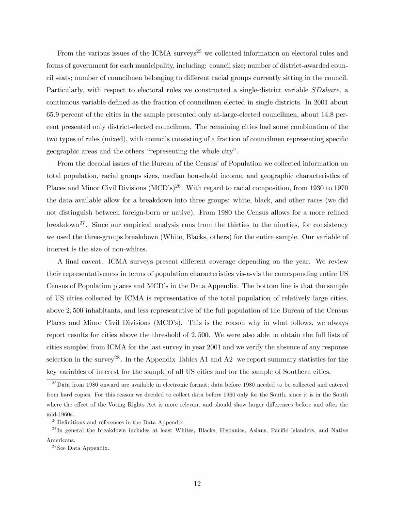
More formally, we establish:
Proposition 1 (a) Both rules AL and SD involve no utility loss to W group individuals when
π ∈¡0, 13 −
α6
¢; (b) if ∆ > δ, then there exists a unique cut-off point bπ ∈ ¡13 − α
6 ,12
¢such that
LALW < LSD
W if π ∈µ1
3− α
6, bπ¶
and
LALW > LSD
W if π ∈µbπ, 1
2
¶;
(c) if ∆ = δ, then for all π ∈¡13 −
α6 ,12
¢the AL rule dominates the SD rule.
Proof. In Appendix.
Figure 1 represents graphically the loss functions LALW and LSD
W where πAL0 (resp. πSD0 ) is the
size of the minority at which the expected loss under AL (resp. SD) becomes positive.
2.4 N districts and mixed systems
We now consider two relevant generalizations of the problem. Suppose that the population is equally
spread over N electoral districts with M individuals in each, which elect a council of size N . We
maintain a distinction between two types of districts: districts with W1 = M and districts with
W2 =¡12 + z
¢M, where Wj denotes the number of whites in a type-j district. Type-1 districts
are all while W2 whereas type-2 districts are an ex ante identical mix of W and B. There are
N1 type-1 districts, therefore N2 = N − N1, and N1 < N2. During the interim phase a mass
αM of B newcomers arrives with α ∼ U [0, α] and α < N. Assume that the W constitutional
writers’ utility u(.) is defined over the share of seats won, where we indicate ∆ = u(1)− u(0) and
7

δ = u(1) − u(N1/N), following the notation of Proposition 1. Proposition 1 then generalizes to
the N− district case: namely, one can show that there exist a first cut-off point πSD0 ∈¡0, 12
¢such
that there is no utility loss for the W group in¡0, πSD0
¢under any rule, and a second cut-off point
π̂ ∈¡πAL0 , 12
¢14 such that expected losses under the two rules AL and SD satisfy
LALW < LSD
W if π ∈ (πSD0 , π̂);LALW > LSD
W if π ∈µπ̂,1
2
¶.
To conclude the section, we now investigate the N−districts case along an important dimension:the opportunity of employing mixed electoral rules for risk-averse W voters. Consider a city with
a council of size NTOT = ρN. Let us now assume ρ > 1 to allow for mixed systems: at least
one representative for each single-member district and NAL > 0 at-large representatives. Assume
W ’s preferences to be defined over the share of seats won on the council. In a setup with risk-
neutral agents, it is never optimal to have mixed systems involving both single-district and at-large
councilmen: either AL or SD offers the highest expected number of winning seats. While a
risk-neutral W considers exclusively the expected seat-share and has no incentives to convexify,
a risk-averse constitutional writer W may find useful to reduce the risk of running pure at-large
elections when the opportunity of winning safer single-district seats is available. The following
proposition presents this result more formally:
Proposition 2 Consider a city of N districts, council of size NTOT , and B newcomers’ arrival
αM, α ∼ U [0, α], N1 < α < N . If the W constitutional writers are risk-averse with utility u(.),
u0 > 0, u00 < 0, defined over the share of seats won, then there is an interval (π3, π4) , π4 < 1/2,
and a mixed system with NSD > 0 single district seats and NAL > 0 at-large seats for which:
UALW < UMX
W and USDW < UMX
W if π ∈ (π3, π4) ,
where UALW is the expected utility under AL, UMX
W is the expected utility under a mixed system,
USDW is the expected utility under SD.
Proof. In Appendix.
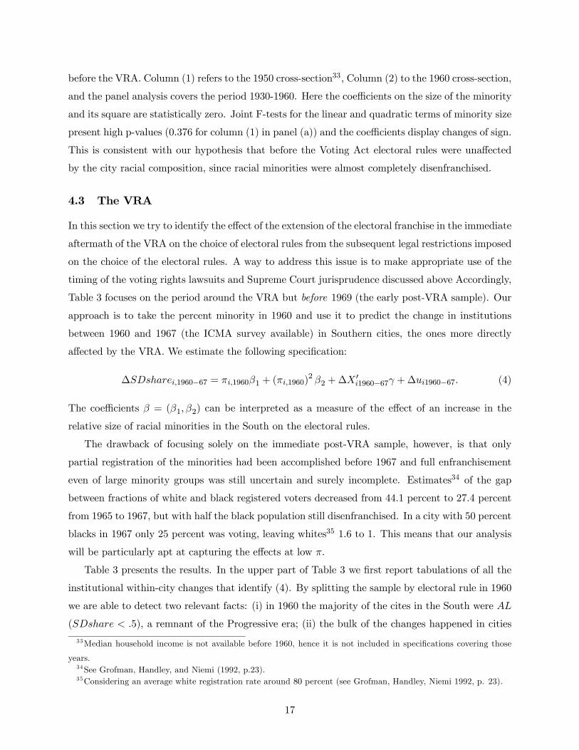
Figure 2 reports a numerical example of the optimal share of single-member district councilmen
as a function of the ex ante size of the minority for a stylized city of N = 12 districts with N1 = 3,
ρ = 5, and W voters with quadratic preferences, as generated by the model. The fundamental
non-linearity in the choice of the electoral rule extends to the case of mixed systems (notice the
ascending part of the step-function that indicates the choice of mixed systems). The parabolic
curve (quadratic fit) that approximates the relation between π and the ratio of SD seats in the
14Where: πAL0 = 12
¡1− α
N
¢> πSD0 = N2
2N
³1− α
N2
´.
8

council (indicated as SDshare) is precisely the relation we will investigate empirically in Section
4. Figure 3 reports the expected utilities for the W agents under the different electoral rules at
various levels of π. The mixed system curve traces the combination of SD and AL seats that is
optimal (i.e. that has the highest expected utility for W ) at any given π. Over the range where
such curve does not coincide with either pure SD or pure AL the chosen electoral rule includes
both single-member district and at-large councilmen.
3 Institutional setting and data
3.1 The Voting Rights Act and its implementation
There was no constitutional protection for voting and electoral participation in the United States
before the Civil War.15 African American individuals in state of servitude were neither granted citi-
zenship nor voting rights. After the war, during the Reconstruction (1867-1877), Congress provided
such constitutional protection with the ratification of the 14th Amendment in 1868 (conferring cit-
izenship to all persons born or naturalized in the United States) and the 15th Amendment in 1870
(providing that the right of vote should not be denied or abridged on the basis of race, color, or
previous status of servitude). It is widely acknowledged that the Reconstruction failed to truly
enfranchise black voters in the South, whose representation in fact went steadily down from the
1870 to the 1960 due to various de facto obstacle to their registration. This does not mean of
course that no black person would vote, but the share of black voters was quite small: in 1868 there
were 300 blacks elected to state legislatures in eleven form confederate states in 1900 there were
516. The Progressive-era (1900-17) fostered substantial institutional innovations in the direction of
reducing representation of minorities. At-large elections were widely introduced both in the South
and in the North with the purported scope of curbing corruption and log-rolling between localized
factional interests, historically represented by SD, but de facto aiming at reducing the influence of
immigrants and (the very few) black voters.
President Lyndon Johnson ratified the 24th Amendment of the Constitution17 (1964) and signed
into law both the Civil Rights Act in 1964 and the Voting Rights Act in 1965. LBJ relied on a
coalition of Northern democrats and republicans to pass the act against the opposition of Southern
15We refer to the United States Department of Justice, Civil Rights Division, Voting Section for further details
and reference for this section.16See in particular the discussion in Kousser (1999) and Grofman and Davidson (1992).17The amendment outlawed the poll tax in federal elections. Virginia ratified the amendment in 1977, albeit
the ratification process was completed on January 23, 1964 (by 38 States). The amendment was ratified by North
Carolina in 1989. The amendment was rejected by the State of Mississippi (and not subsequently ratified) in 1962.
9

democrats. The goal of the VRA is to remove obstacles in voting registration procedures for racial
minorities. Section 2 of the Act included a broad reassessment of the principles embedded in
the 14th and 15th Amendments. It deemed illegal the use of poll taxes, literacy tests, and the
requirement of fluency in English for voting eligibility. As a consequence of the Voting Rights
Act, the number of registered minority voters as a fraction of voting age population doubled and in
some cases tripled in Alabama, Georgia, Louisiana, Mississippi, and Virginia between 1965 and 1988
(Grofman, Handley and Niemi, 1992)18. Even though white Southerners grudgingly had to remove
obstacles to black registration (penalty was jail) they immediately started trying to change electoral
laws in order to minimize the probability of electing black representatives. For instance already
in January 1966 an all-white legislature in Mississippi without much discussion and unanimously
passed 13 bills concerning the election process, most of them moving various type of elections to an
at large system19. The purpose was clearly to dilute black votes. Eventually in 1969 in Allen vs.
State Board of Election the Supreme Court struck down most of these bills. In fact the mid sixties
mark the beginning of a long series of court battles about vote diluting, gerrymandering, and various
other maneuvers of the white majority to minimize black influence. Different lower courts ruled
in different ways and there was much uncertainty about how each specific ruling would go given
the complexity of the issues involved20. Because of all these disagreements in the lower courts, the
Supreme Court in 1980 took on the Case of City of Mobile versus Bolden and established the need
to prove discriminatory purposes when challenging a change in electoral rules21. The language
of the majority opinion suggested very high standard of proof for active discrimination22. In a
18Amy (2002) reports that “the number of black elected officials in the United States grew an average 16.7 percent
a year between 1970 and 1977, from 1469 to 4311” (p.129). In 1999 according to the Joint Center for Political and
Economic Studies the total number of black elected officials was 5938 in the South (respectively 8936 in all U.S.),
of which 340 were city mayors (resp. 450 nationwide), 2677 members of municipal governing bodies (resp. 3498
nationwide). There were no black senators in 1999 and 19 representatives form the South (39 black representatives
nationwide). See also Cole (1976).19See the detailed discussion by Parker (1990).20For a revealing review of extremely different point of views held by opposing expert witnesses in the cases see
Grofman (1992) in Grofman and Davidson (1992)21 In 1980 the Supreme Court imposed the requirement of proof of “racial discriminatory purpose” in vote dilution
cases (Mobile v. Bolden, 446 U.S. 55, 1980). This was rectified by a 1982 Congress Amendment, dispensing from
such proof. The Supreme Court substantially challenged “affirmative gerrymandering” in Shaw v. Reno, 509 U.S.
630 (1993) and Holden v. Hall, 512 U.S. 874 (1994) among the others. Under President Bill Clinton the National
Voter Registration Act (also known popularly as the Motor Voter Act of 1993) aimed at strongly promoting voter
registration (for example, through the department of motor vehicles structures, unemployment, and welfare bureaus).
More recently the Help America Vote Act of 2001 has shifted back to individual States most of the supervisory power
over the quality of electoral franchise. Voting Rights Acts renewal hearings are due in 2007.22See Grofman, Handley, and Niemi (1992).
10

reaction to this ruling a 1982 Congress Amendment, dispensed from such proof. Finally in 1986
in the ruling of Thornbourg versus Gingles the Supreme Court clarified what had to be considered
active discrimination in a series of points including the presence of block voting, a history of racial
discrimination, evidence of vote diluting, gerrymandering, etc. While the court did clarify the
issue, still a very large grey area persisted. For instance, as our model itself suggests, the fact
that moving to at-large election may dilute black votes, but sometimes moving to single-member
districts may disadvantage blacks as well was already in the minds of litigants in the seventies,
eighties and nineties (see Chapter 5 of Grofman Handley and Niemi (1992)). Also it was not clear
how many of the points were necessary and/or sufficient to prove discrimination. This is not a
failure of the Court per se, but just reflects the complexity of the issues at hand.
From this brief historical excursus, we need to remember three points germane to our empirical
analysis: 1) Until the mid-sixties white majorities did not have to worry about black vote in
the South; only with the Voting Act of 1965 blacks were really a political block to reckon with
electorally. 2) The implementation by the Courts of the Voting Rights Act also took up the issues
of the choice of electoral rules, precisely to avoid choices (like at-large elections) that would have
favored the white majority. 3) Attempts of the white majority to change electoral laws were kept
in check by the Courts which became increasingly concerned. But at least well into the eighties
and even beyond that much uncertainty remained about what could or could not be challenged in
courts. So a fair amount of room for maneuver remained for the white majority to strategically
manipulate electoral rules. In a sense, without courts interventions our finding below would be
even stronger, since the white majority could have acted unconstrained.
3.2 Data and summary statistics
This section briefly reviews the main variables employed in the empirical analysis. We refer the
reader to the separate Data Appendix23 for details on variables definition, construction, and sources.
We gathered two sets of data: one including characteristics of city governments and their institu-
tional details; the other including demographic, economic, and geographic characteristics of US
cities. We collected information on US municipal governments characteristics for the period 1930-
2000, at 10-year intervals, from the Form of Government Survey and Municipal Year Book by the
International City/County Management Association (ICMA) in Washington D.C.24
23Due to space limitations we produce the Data Appendix in a separate document, available on request. Please
refer to the authors’ webpages for a downloadable version of the Data Appendix.24 ICMA is a professional organization of city managers and administrators publishing local government data since
1914 and a recognized scholarly source. ICMA data have been employed in a number of papers, including Baqir
(2002), Sass and Pittman (2000), DeSantis and Renner (1992) among the others.
11
From the various issues of the ICMA surveys25 we collected information on electoral rules and
forms of government for each municipality, including: council size; number of district-awarded coun-
cil seats; number of councilmen belonging to different racial groups currently sitting in the council.
Particularly, with respect to electoral rules we constructed a single-district variable SDshare, a
continuous variable defined as the fraction of councilmen elected in single districts. In 2001 about
65.9 percent of the cities in the sample presented only at-large-elected councilmen, about 14.8 per-
cent presented only district-elected councilmen. The remaining cities had some combination of the
two types of rules (mixed), with councils consisting of a fraction of councilmen representing specific
geographic areas and the others “representing the whole city”.
From the decadal issues of the Bureau of the Census’ of Population we collected information on
total population, racial groups sizes, median household income, and geographic characteristics of
Places and Minor Civil Divisions (MCD’s)26. With regard to racial composition, from 1930 to 1970
the data available allow for a breakdown into three groups: white, black, and other races (we did
not distinguish between foreign-born or native). From 1980 the Census allows for a more refined
breakdown27. Since our empirical analysis runs from the thirties to the nineties, for consistency
we used the three-groups breakdown (White, Blacks, others) for the entire sample. Our variable of
interest is the size of non-whites.
A final caveat. ICMA surveys present different coverage depending on the year. We review
their representativeness in terms of population characteristics vis-a-vis the corresponding entire US
Census of Population places and MCD’s in the Data Appendix. The bottom line is that the sample
of US cities collected by ICMA is representative of the total population of relatively large cities,
above 2, 500 inhabitants, and less representative of the full population of the Bureau of the Census
Places and Minor Civil Divisions (MCD’s). This is the reason why in what follows, we always
report results for cities above the threshold of 2, 500. We were also able to obtain the full lists of
cities sampled from ICMA for the last survey in year 2001 and we verify the absence of any response
selection in the survey28. In the Appendix Tables A1 and A2 we report summary statistics for the
key variables of interest for the sample of all US cities and for the sample of Southern cities.
25Data from 1980 onward are available in electronic format; data before 1980 needed to be collected and entered
from hard copies. For this reason we decided to collect data before 1960 only for the South, since it is in the South
where the effect of the Voting Rights Act is more relevant and should show larger differences before and after the
mid-1960s.26Definitions and references in the Data Appendix.27 In general the breakdown includes at least Whites, Blacks, Hispanics, Asians, Pacific Islanders, and Native
Americans.28See Data Appendix.
12

4 Empirical results
We now focus on the main prediction of our model, namely that: the preference of constitution
writers for AL over SD, increases and then decreases with the initial size of the minority group.
This section presents the main results.
4.1 The choice of electoral rules
Empirical Strategy - The empirical strategy that we employ in Table 1 and in the majority of the
following tables is a simple, yet flexible, linear (in the coefficients) parametric model of the choice
of electoral rules. Proposition 1 hypothesizes a non-monotonic, U−shaped relationship betweenSDshare (the fraction of councilmen elected by ward or district) and π (the size of the minority),
which provides intuitive appeal to the choice of fitting a quadratic relationship. For each city i in
year t let us define the electoral rule variable, SDshareit, the relative size of the minority, πit, a
vector of (k x 1) controls Xit, in our baseline specification: the log of city population and median
household income. We specify the following equation in levels:
SDshareit = β0 + πitβ1 + (πit)2 β2 +X 0
itγ + uit (3)
for i = 1, ..., N and t = 1, ..., T .
We perform our analysis both in a cross-section for given t and in a two-way panel in which we
account for unobserved, time-invariant heterogeneity at the city level and for time-specific effects29.
In the latter case the two-way error component becomes uit = αi + δt + ηit. Controlling for city-
specific unobserved characteristics is relevant to our empirical strategy. Historical, geographical,
and cultural conditions explain much of the variation in political institutions at the city cross-
sectional level (about 67 percent of the variation on average). However, such conditions are often
difficult to measure directly and may bias, if omitted, any cross-sectional inference concerning the
role of changes of racial composition of the city in the choice of electoral rules. Employing within-
city variation allows us to account for such unobserved heterogeneity and estimate consistently the
vector β = (β1, β2) . Time-specific effects are similarly useful in accounting for across-the-board
effects, such as federal legislation, that again need to be controlled for, especially in the post-1965
period when legislation was extremely active. We address the issue of serial correlation in the
error component η by relaxing the assumption of independence and clustering at the city level.
Conditional heteroskedasticity of unknown type is also accounted for in all standard errors both in
the cross-section and the panel results.29Formal F-tests for this specification support the use of a two-way setup. Both groups of fixed effects are jointly
significant in every specification.
13

Identification - The most likely source of reverse causation affecting (3) is endogenous sorting
across municipalities driven by more favorable electoral rules. Minority voters may move towards
cities in which they have better chances of representation, and similarly white voters may move
out of cities with excess minority representation. In general, Tiebout sorting would predict a
correlation between changes in city racial composition and in electoral rules of the opposite sign to
what predicted by our model, dampening the least squares estimates towards zero.
To see this, suppose that, given a small size of the minority, π, a city changes its electoral rule
in favor of white voters against black voters by decreasing the number of single-district seats on the
council. In this case Tiebout sorting would predict a decrease in the size of the minority (blacks
would leave the city and possibly more whites could join in), implying a positive correlation between
the share of single-district seats and the size of the minority at small π. Now suppose that, given
a large size of the minority, π, a city changes its electoral rule by increasing the number of single-
district seats on the council. Under the basic setup of Proposition 1 this produces an unambiguous
reduction of the expected utility of the blacks. Tiebout sorting would predict a decrease in the size
of the minority (blacks would leave the city and possibly more whites could join in), implying a
negative correlation between the share of single-district seats and the size of the minority at large
π. However, it is enough to move to our more general theoretical setup including risk aversion to
see that moving towards single-member district at high π may produce an increase in the utility of
both groups. In this case Tiebout sorting could produce an overestimate of the true slope of the
U− curve in the rightmost range of π.We address potential endogeneity by instrumenting the fraction of the minority with 10 years
lags and geographic location (an indicator variable taking value 1 if the city is in geography).
Distant lags and geographic location should be considered predetermined or exogenous (the case
for South) and therefore valid instruments of current size of the minority. Exclusion restrictions
can be tested given overidentification of the system.
Results - Table 1, panel (a), presents the results concerning the main non-monotonicity. The
Table refers to the sample of US cities30 in 1990 for the cross-sectional analysis (in columns 1-
3) and to the period 1970-2000 for the panel analysis (columns 4 and 5). The model calls for a
negative linear and a positive quadratic coefficient on the share of the non-white minority31. The
30As for all the rest of our empirical analysis we exclude from the sample those cities for which we have information
that the change of structure of government is the result of court mandate or State Law. We also exclude cities below
2500 as the ICMA sample is representative of the US Census of Population places and MCD in this group. Similar
results were obtained when employing the complete sample of municipalities or performing the cross-sectional analysis
for the years 1980 and 2000.31Note that one may want to exclude cities in which whites are a minority. There are very few of those and
14

signs of the coefficients are consistent with this story and significant at standard confidence levels
both individually and jointly. Looking at column (1) the estimated coefficients imply that the U−shaped curve reaches a minimum (indicated with π∗) at about 43.8 percent non-white minority.
(Note that 94.5 percent of the cities in year 1990 were below this level). In column (2) we include
for robustness a larger set of controls, of which we do not report the coefficients. For column (2) the
controls are: the squared log of city population and income, the fraction of population employed
in manufacturing, agriculture, mining, trade, financial services, and fraction above 65 years of age.
The estimated coefficients support qualitatively the results of column (1) with a lower minimum at
0.388 and are again individually and jointly significant.
Column (3) reports 2SLS estimates of the specification in column (1). Consistently with our
previous discussion concerning identification, the coefficients on the linear and quadratic terms
become larger in absolute value and outside the 95 percent confidence interval for the estimates of
column (1). This finding seems to suggest a reduction of the possible attenuation bias stemming
from Tiebout sorting. A J-test for overidentification of all instruments produces a p-value of 0.12,
thus not rejecting the validity of the instruments set in terms of exclusion restrictions. It is a low
value, however, given the low power properties of the test. The minimum for the U− shaped curveis estimated at 0.318 minority size.
In columns (4) and (5) we tackle the issue of unobserved heterogeneity at the city level in our
baseline specification and in one where additional controls are added. For column (5) controls are
the squared log of city population and median income. We obtain estimates of β = (β1, β2) close to
the 2SLS estimates and statistically significant at the 1 percent confidence level (both individually
and jointly).
To gauge quantitatively the size of the two effects in Table 1, we can start from the empirical
distribution of minorities in US cities in year 1990 for the cities in our sample32. The median (Q5)
for the fraction of minority is 5.5 percent and the ninth decile (Q9) is 34.3. At Q5, given estimated
coefficients in column (4) of −0.622 and 1.078 (with robust standard errors respectively 0.202 and0.284), an increase of one standard deviation of minority sizes (15.3 percent) implies a reduction of
−5.3 percent of the fraction of single-district seats. This is equivalent to about 1/3 seat switchingfrom single-member district to at-large in a council of 6 seats (the mean council size in the 1990
sample). At Q9, the same increase of one standard deviation would instead produce an increase of
about +4.4 percent in the fraction of single-district seats. This would be equivalent to more than
in addition even when whites are a minority in terms of number of inhabitants, demographic factors and vote
participation patterns may still make them a majority as active voters (see Amy 2002 for an example). For this
reason it is unclear which cities to drop from the sample. We tried a few experiments and our results appear robust.32But likewise for the decades 1980, 2000.
15

1/4 seat switching from at-large to single-district in a council of 6 seats.
The estimates are quantitatively reasonable, since the voting rights legislation over the years
has imposed increasing limits on institutional changes. In other words, without Supreme Court
involvement, these effects would have been surely larger. We return to this issue below. To
conclude, in its lower portion (panel b) Table 1 presents estimates employing a (two-sided) limited
dependent variable (LDV) approach, a Tobit and IV Tobit estimator for columns (1)-(3) and a
random effects Tobit estimator grouping observations at the city level for columns (4)-(5). This is
a way of incorporating the empirical feature that SDshare is constrained to be in [0, 1]. All the
specifications correspond to the ones of panel (a). The implications of panel (a) carry over to LDV
specification consistently with the predictions of Proposition 1.
We also separately run a battery of robustness checks that we do not report for the sake of syn-
thesis. We have considered a discrete version of our dependent variable, SD, and found analogous
evidence of the main non-monotonicity for both the cross-section and the panel (using conditional
logit fixed effects). Since time dependence is an important characteristic of political systems, we
have included the t−10 lag of SDshare and employed a standard dynamic panel technique, through
first differencing and application of the Arellano and Bond (1991) GMM estimator. The consistency
of the standard linear model and this dynamic extension are source of reassurance. The dynamic
model delivers stronger effects, in the range of 1/2 seat in a council of 6 (towards and away from
AL), especially for the South. We have also considered a simple non-parametric approach, ex-
pecting to observe two basic regularities in the data. First, the slope of a within regression of the
single-district variable on the fraction of the minority should be increasing in subsamples where the
average minority size is increasingly higher. Second, we would expect statistically significant coeffi-
cients of negative sign to appear at relatively small values of the fraction of the minority (where the
steeper downward-bending part of the U) and statistically significant coefficients of positive sign
to appear at relatively large values of the fraction of the minority (steeper upward-bending part of
the U). A flat and insignificant relationship should appear in the middle range. Both regularities
seem supported by the data.
4.2 Before the VRA
An important issue in the empirical strategy concerns the timing of the Voting Rights Act. We
employ such date as an informative source of variation for institutional manipulation. Table 2
reproposes the specifications of columns (1) and (4) of Table 1 before the Voting Rights Act of
1965. The top (OLS) and bottom (Tobit) panels show regressions for the sample of Southern cities
16
before the VRA. Column (1) refers to the 1950 cross-section33, Column (2) to the 1960 cross-section,
and the panel analysis covers the period 1930-1960. Here the coefficients on the size of the minority
and its square are statistically zero. Joint F-tests for the linear and quadratic terms of minority size
present high p-values (0.376 for column (1) in panel (a)) and the coefficients display changes of sign.
This is consistent with our hypothesis that before the Voting Act electoral rules were unaffected
by the city racial composition, since racial minorities were almost completely disenfranchised.
4.3 The VRA
In this section we try to identify the effect of the extension of the electoral franchise in the immediate
aftermath of the VRA on the choice of electoral rules from the subsequent legal restrictions imposed
on the choice of the electoral rules. A way to address this issue is to make appropriate use of the
timing of the voting rights lawsuits and Supreme Court jurisprudence discussed above Accordingly,
Table 3 focuses on the period around the VRA but before 1969 (the early post-VRA sample). Our
approach is to take the percent minority in 1960 and use it to predict the change in institutions
between 1960 and 1967 (the ICMA survey available) in Southern cities, the ones more directly
affected by the VRA. We estimate the following specification:
∆SDsharei,1960−67 = πi,1960β1 + (πi,1960)2 β2 +∆X
0i1960−67γ +∆ui1960−67. (4)
The coefficients β = (β1, β2) can be interpreted as a measure of the effect of an increase in the
relative size of racial minorities in the South on the electoral rules.
The drawback of focusing solely on the immediate post-VRA sample, however, is that only
partial registration of the minorities had been accomplished before 1967 and full enfranchisement
even of large minority groups was still uncertain and surely incomplete. Estimates34 of the gap
between fractions of white and black registered voters decreased from 44.1 percent to 27.4 percent
from 1965 to 1967, but with half the black population still disenfranchised. In a city with 50 percent
blacks in 1967 only 25 percent was voting, leaving whites35 1.6 to 1. This means that our analysis
will be particularly apt at capturing the effects at low π.
Table 3 presents the results. In the upper part of Table 3 we first report tabulations of all the
institutional within-city changes that identify (4). By splitting the sample by electoral rule in 1960
we are able to detect two relevant facts: (i) in 1960 the majority of the cites in the South were AL
(SDshare < .5), a remnant of the Progressive era; (ii) the bulk of the changes happened in cities
33Median household income is not available before 1960, hence it is not included in specifications covering those
years.34See Grofman, Handley, and Niemi (1992, p.23).35Considering an average white registration rate around 80 percent (see Grofman, Handley, Niemi 1992, p. 23).
17

where SDshare > .5. In the South basically all cities employing an AL rule kept it unchanged
at the moment of the black enfranchisement and a vast majority of the SD cities moved towards
at-large in a way consistent with intuition and our model. If a city moves from zero voting minority
(where the electoral rule is inconsequential) to π < π∗, the only type of city that should change is
the (initially) SD moving towards AL. The AL cities should not move unless π is very large. It is
therefore not surprising that our results will be especially strong concerning the movement towards
AL.
Column (1) in the bottom part of Table 3 presents first-difference estimates for the specification
(4), where the fraction of the minority enters linearly at the 1960 level and in a quadratic form.
The estimated coefficient β1 presents the expected sign but not β2, and both are not statistically
significant. In column (2) we run the same regression in the portion of the data containing the
identifying information: the initially SD cities. Importantly the regression picks up both the linear
and the quadratic effects in a way consistent with the theory. Similarly to Section 4.1 we can
calculate the effect of an increase of one standard deviation of minority sizes (0.153). The effects
are −23.2 (at Q5) and +4.1 percent (at Q9) of the share of single-member seats. The negative effectis around four times larger than in Table (1), confirming substantial pressure towards endogenous
changes in the electoral rules. In column (3) we restrict to the set of initially AL cities. Here
identification is due to a very small fraction of cities, the few changing, and we find a counterintuitive
swap in coefficients signs and borderline significance for the t-tests. Notice however that these
findings are countervailed by lack of joint significance of π and π2, a result consistent with the
model. The F-test p-value does not warrant rejection at any standard confidence level.
It is also relevant to investigate how our results would change depending on the VRA coverage.
In columns (4)-(6) we run the same specifications of columns (1)-(3) on the VRA-fully covered
states with stronger results than in the overall South sample. Estimates especially differ on the
quantitative implications on the increasing part. Repeating our calculations, the two estimated
effects are now −23.5 percent at Q5 and +11 percent at Q9 for the sample of cities initially SD.
Again we detect individual but no joint significance of π and π2 for the AL cities (the F-test p-value
does not warrant rejection at any standard confidence level).
The immediate post-VRAmovement toward at-large seems therefore consistent with the downward-
sloping component of the main non-monotonicity, but the increasing part of the parabola is also
present in the part of the data where the identifying information is. Finally, repeating the estima-
tion for the fraction of blacks in 1960 produces analogous results.
18

4.4 Minority representation
Our basic story holds that electoral rules affect the ratio of minorities elected differently. This is
the reason why the constitutional writers choose different rules in the first place. Crucially, the
ratio of non-white council members should display dependence on the electoral rules in order for
the fundamental tenet of our analysis to be verified. Moreover, different rules should have different
effects on minority representation at different minority sizes. By quantitatively documenting the
correlation between electoral rules and minority representation, in this section we provide evidence
that both statements are verified by the data and that the estimated effects move in the direction
our model rationalizes.
The representational ratio (RR) is the fraction of minority councilmen in a council divided by the
fraction of the population that belongs to the minority and is available for our all-US cities sample
in year 1980, 1990, and 200036. We regress RR on our variable of interests, the single-district rule
variable. Table 4 reports the results. The null hypothesis that the electoral rule adopted by a city
has no association with the representational ratio is soundly rejected in both a 1990 cross-sectional
regressions (Panel a, column 1) and in fixed-effect regressions in which time invariant city-specific
unobserved heterogeneity is accounted for (Panel b, column 1)37. Single-district rules substantially
increase the chance of minorities to be proportionally represented at the municipal level. Recalling
that the fraction of single-district seats, SDshare, is defined over the [0, 1] interval, our results in
column (1) imply an average increase in the RR of the city council between 8.2 (in panel a) and
21.6 (in panel b) percent from switching from a fully at-large rule to a fully single-district rule. This
is a quantitatively substantial effect: each black or minority vote has more than 1/5 more weight
in terms of electoral representation under single-district than under at-large elections38. Finally,
let us note that the correlations presented in column (1) identify the effect of the electoral rule on
the representational ratio without the strong exclusion restriction that the fraction of the minority
has an independent effect on RR.
In columns (2)-(4) we provide evidence that the impact of the single-district rule on the repre-
36Very few cities for the all US sample present representational ratios of minorities of more than 1, indicating
over-proportional representation. Even less of them are present in the South. In order to limit the role of these
outliers we limit the representational ratio to be smaller than 5.37All panel specifications include year fixed effects and a set of standard controls for city size (log population) and
income levels (log household median income in 1990 dollars) and we apply the same clustering as Table 1.38Focusing on the South produces even stronger estimates, in a range of 1/3. Sass and Pittman (2000) also provide
panel data evidence on the effect of electoral rule on minority representation reporting a representational ratio
differential of 36 percent, larger but comparable with our estimates. Our results extend to more recent data and a
substantially larger sample of cities.
19

sentational ratio is actually non-monotonic in the size of the minority by looking at the effect of
the single-district variable over different ranges of π.
At low levels of minority size both at-large and single-district should be indistinguishable in
warranting representation: minority are just too small to achieve representation under any rule.
However, as the minority size increases single-district will offer better chances of representation to
geographically segregated minorities vis-a-vis at-large. Such effect will diminish, however, when the
minority becomes so large that some district votes (those beyond simple majority in the district)
will be wasted (particularly, when π is above the estimated π∗). This implies that the sign of the
coefficient should be the highest in intermediate ranges of π and the lowest when the fraction of
the minority is either very small or very large. The three ranges we employ are: (i) below the mean
of π;39 between the mean and the minimum, π∗, of the U computed in Table 1 (columns 1 for the
cross-section and 4 for the panel); and above π∗.
In panel (a) columns (2)-(4) present coefficients suggestive of the implied non-monotonicity.
Single-district maintains its expected positive effect, but its effect is quantitatively always stronger
at intermediate ranges. A similar picture arises in the fixed effect analysis of panel (b). Notice that
the effect of SDshare is consistently significant and large in both the cross-section and the panel
only at intermediate ranges of π. The results are influenced by the choice of the thresholds, but the
decreasing effect of SDshare seems to be a robust feature of the data.
We are not the first to observe that at-large election favors the white majority but we are not
aware of previous empirical studies pointing at the non-monotonicity in the effect of single-district
rules on minority representation.
5 Conclusions
Before the Voting Rights Act of 1965, racial minorities were essentially disenfranchised in the US
South. Therefore, the type of electoral institutions were irrelevant in determining the level of control
of the white majority: a level of control that was almost absolute. The Voting Rights Act allowed
racial minorities to enter into the political arena. The white majorities reacted, within the legal
boundaries of the Voting Rights Act, by changing electoral rules as to minimize expected minority
influence. This evidence suggests how institutions (in this case electoral rules) evolve even rather
quickly in response to changes in the environment and raises questions about empirical evidence
that holds electoral institutions as exogenous.
39The mean π for the 1990 sample is 0.125 and for the panel is 0.130.
20

References
[1] Aghion, Philippe, Alberto Alesina, and Francesco Trebbi (2004) “Endogenous Political Insti-
tutions” Quarterly Journal of Economics, 119, May, 565- 612.
[2] Aghion, Philippe and Patrick Bolton (2003) “Incomplete Social Contracts” Journal of the
European Economic Association,1, 38-67.
[3] Alesina, Alberto, Reza Baqir, and Caroline Hoxby (2004) “Political Jurisdictions in Heteroge-
neous Communities” Journal of Political Economy, 112, April, 348-396.
[4] Alesina, Alberto and Edward Glaeser (2004) Fighting Poverty in the US and Europe: A World
of Difference (Oxford University Press, Oxford, UK).
[5] Alesina, Alberto and Howard Rosenthal (1995) Partisan Politics, Divided Government, and
the Economy (Cambridge University press, Cambridge, UK).
[6] Alexander, Gerard (2004) “France: Reform-mongering between Majority Runoff and Pro-
portionality”, in Handbook of Electoral System Choice, by Josep M. Colomer (ed.) (Palgrave
MacMillan, New York, N.Y.)
[7] Alt, James E. and Robert C. Lowry (1994) “Divided Government, Fiscal Institutions and
Budget Deficits: Evidence from the States” American Political Science Review, 89, December,
811-828.
[8] Amy, Douglas J. (2002, second edition) Real Choices / New Voices: The Case for Proportional
Representation Elections in the United States (Columbia University Press, New York, NY).
[9] Arellano, Manuel and Stephen Bond (1991) “Some Tests of Specification for Panel Data: Monte
Carlo Evidence and an Application to Employment Equations” Review of Economics Studies,
58, January, 277-297.
[10] Baqir, Reza (2002) “Districting and Government Overspending” Journal of Political Economy,
110, December, 1318-1354.
[11] Bohn, Henning and Robert P. Inman (1996) “Balanced Budget Rules and Public Deficits:
Evidence from US States” Carnegie Rochester Conference on Public Policies, 13-76.
[12] Buchanan, James M. and Gordon Tullock (1962) The Calculus of Consent: Logical Foundations
of Constitutional Democracy (University of Michigan Press, Ann Arbor, MI).
21

[13] Cameron, Charles, David Epstein, and Sharyn O’Halloran (1996) “Do Majority-Minority Dis-
tricts Maximize Substantive Black Representation in Congress?” American Political Science
Review, 90, 4, December, 794-812.
[14] Cole, Leonard A. (1976) Blacks in Power: A Comparative Study of Black and White Elected
Officials (Princeton University Press, Princeton, NJ).
[15] Colomer, Josep M. (2004) Handbook of Electoral System Choice, (Palgrave MacMillan, New
York, N.Y.)
[16] Cox, Gary W. and Johnatan N. Katz (2002) Elbridge Gerry’s Salamander (Cambridge Uni-
versity press, Cambridge, UK).
[17] Cutler, David, Edward Glaeser, and Jacob Vigdor (1999) “The Rise and Decline of the Amer-
ican Ghetto”, Journal of Political Economy, 107, June, 455-506.
[18] DeSantis, Victor and Tari Renner “Minority and Gender Representation In American County
Legislatures: The Effect of Election Systems” in Rule, Wilma and Joseph F. Zimmerman (eds.)
(1992) United States Electoral Systems (Greenwood Press, New York, US).
[19] Epple, Dennis and Thomas Romer (1991) “Mobility and Redistribution” Journal of Political
Economy, 99, August, 828-858.
[20] Friedman, John N. and Richard Holden (2005) “Towards a Theory of Optimal Partisan Ger-
rymandering” Mimeograph, Harvard University.
[21] Grofman, Bernard, Lisa Handley, and Richard Niemi (1992) Minority Representation and the
Quest for Voting Equality (Cambridge University Press, New York, NY).
[22] Grofman B. and C. Davidson (1992) Controversies in Minority Voting Borrikings Institution
Washington DC
[23] Hacker, Andrew (1992) Two nations: Black and White, Separate, Hostile, Unequal (Scribner’s,
New York, US).
[24] Hayek, Friedrich A. (1960) The Constitution of Liberty (University of Chicago Press, Chicago,
Ill).
[25] Huckfeld, Robert, and Carol Weitzel Kohfeld (1989) Race and the Decline of Class in American
Politics (University of Illinois Press, Urbana, Ill).
22

[26] Karning, Albert K. and Susan Welch (1982) “Electoral Structure and Black Representation
on City Councils” Social Science Quarterly, 63, March, 99-114.
[27] Kousser, Morgan J. (1999) Color-blind Injustice: Minority Voting Rights and the Undoing of
the Second Reconstruction (University of North Carolina Press, Chapel Hill, NC).
[28] Kreuzer, Marcus (2004) “Germany: Partisan Engineering of Personalized Proportional Rep-
resentation”, in Handbook of Electoral System Choice, by Josep M. Colomer (ed.) (Palgrave
MacMillan, New York, N.Y.)
[29] Laffont, Jean-Jacques (2000) Incentives and Political Economy (Oxford University Press, New
York, NY).
[30] Lijphart, Arend (1994) Electoral Systems and Party Systems: a Study of 27 Democracies
(Oxford University Press, New York, NY).
[31] Lipset, Seymour .M. and Rokkan, Stein (1967) Party Systems and Voter Alignments. New
York: Free Press.
[32] Mulligan, Casey B., Richard Gil, and Xavier Sala-i-Martin (2004) “Do Democracies Have
Different Public Policies than Nondemocracies?” Journal of Economic Perspectives, 18, winter,
51-74.
[33] Pande, Rohini (2003) “Can Mandate Political Representation Increase Policy Influence for
Disadvantaged Minorities? Theory and Evidence from India” American Economic Review,
93, 1132-1151.
[34] Parker F. (1990) Black Votes Count: Poltical Empowerement in Mississipi After 1965 Univer-
sity of North carolina press, Chapell Hill NC
[35] Persson, Torsten and Guido Tabellini (2003) The Economics Effects of Constitutions (MIT
Press, Cambridge, MA).
[36] Poterba, James M. (1994) “State Response on Fiscal Crises: The Effects of Budgetary Insti-
tutions on Policies”, Journal of Political Economy, 102, August, 799-821.
[37] Riker, William (1986) The Art of Political Manipulation (Yale University Press, New Haven,
CT).
[38] Sass, Tim R. and Bobby J. Pittman (2000) “The Changing Impact of Electoral Structure on
Black Representation in the South, 1970-1996” Public Choice, 104, 3-4, September, 369-388.
23

[39] Strumpf, S. Koleman and Felix Oberholzer-Gee (2002) “Endogenous Policy Decentralization:
Testing the Central Tenet of Economic Federalism” Journal of Political Economy, 110, Febru-
ary, 1-36.
[40] Voigt, Stefan (1997) “Positive Constitutional Economics: A Survey” Public Choice, 90, March,
11-53.
[41] Wilson,William J. (1996)When Work Disappear: The World of the New Urban Poor (Knopf,
New York, NY)
24

6 Appendix: Proofs of Propositions
Proof of Proposition 1
Part (a) is straightforward. For part (b) consider that:
LALW = 0 < LSD
W if π ∈µ1
3− α
6,1
2− α
6
¶;
and LALW and LSD
W are both linear increasing in π for π ∈¡12 −
α6 ,13
¢.At π = 1
3 , we may have two
cases. Case 1: it holds that
LALW =
µ1− 1
α
¶∆ > LSD
W = δ
and hence the existence of a unique cut-off bπ ∈ ¡12 − α6 ,
13
¢with the desired properties. Case 2:
∆
µ1− 1
α
¶≤ δ and ∆ > δ.
For π ∈¡13 ,12
¢the loss LAL
W is linear increasing in π and LSDW is constant at δ. Hence the existence
of a unique cut-off bπ ∈ ¡13 , 12¢ in this case. Finally, to establish part (c) consider that for any π
between 0 and 12 , we have:
LSDW ≥ LAL
W
since here ∆ = δ and µ1− 2
α(1− 3π)+
¶+≥µ1− 3
α(1− 2π)
¶+. (5)
At π = 12 (5) holds with equality. This establishes the proposition.
Proof of Proposition 2
Define N1/N = n1 and ρ = NTOT/N. Normalize u(0) = 0. The expected utility of a pure AL
is:
UALW = Pr(α < X)u(1),
where X (π) = N (1− 2π) .The probability under a single-member district system of winning type-2 districts 1, 2, ..., N2
for W is:
Pr
µα <
(1− 2πN/N2)
f
¶With constant f = 1/N2 indicate Y (π) =
(1−2πN/N2)+f = (N2 − 2πN)+ . Then the expected utility
of pure SD for given π is:
USDW = Pr(α > Y )u(n1) + Pr(α < Y )u(1).
Notice that X (π) > Y (π) , ∀π.
25

Consider the value of π∗ at which the expected share of seats won by W is the same under pure
AL and pure SD. For any π < π∗, AL is actuarially more favorable than SD. If W is risk averse,
the π̂ at which USDW = UAL
W lays in the interval¡πAL0 , π∗
¢, since AL is a riskier electoral rule. A
unique point π̂ always exists as shown in the text. It follows that
USDW = UAL
W (6)
=⇒ Pr(α > Y ) = Pr(Y < α < X)u(1)
u(n1),
where
Pr(α > Y ) = 1− (N2 − 2πN)+ /α
Pr(Y < α < X) = N1/α
Hence (6) implies that at π̂ :
u(1)
u(n1)=
α
N1− 1
N1(N2 − 2π̂N)+ <
α
N1<
N
N1(7)
A risk averse W will always accept at least a small amount of risk that is actuarially favorable.
Therefore, at π̂ W will prefer a mixed system to a pure SD rule.
To see this, define the number of SD councilmen per district ρ and consider the problem of W
for π = π̂ :
maxρ
©UMXW (ρ)
ªsubject to 0 ≤ ρ ≤ ρ.
The expected utility of a mixed system MX for given π is:
UMXW = Pr(α > X)u(ρn1/ρ) + Pr(Y < α < X)u
¡¡ρn1 + ρ− ρ
¢/ρ¢
(8)
+Pr(α < Y )u(1)
By using the expression in (8) and allowing ρ to take continuous values the FOC for the problem
is:
Φ(ρ) =1
ρ
£n1 Pr(α > X)u0(ρn1/ρ)− (1− n1) Pr(Y < α < X)u0
¡¡ρn1 + ρ− ρ
¢/ρ¢¤.
Consider Φ(ρ) at π = π̂ :
Φ(ρ) =Pr(Y < α < X)
ρN∗ (9)∙
N1
µu(1)
u(n1)− 1¶u0(ρn1/ρ)−N2u
0 ¡¡ρn1 + ρ− ρ¢/ρ¢¸
.
26

where we use the fact that Pr(α > X) = Pr(α > Y )− Pr(Y < α < X) and condition (6). We are
interested in evaluating (9) at ρ = ρ :
Φ(ρ = ρ) =Pr(Y < α < X)
ρNu0(n1)
∙N1
µu(1)
u(n1)− 1¶−N2
¸. (10)
By replacing in (10) the expression in (7) we can see that the FOC is strictly negative at ρ = ρ.
This is because the element in brackets in (10) is strictly negative by (7):
N1u(1)
u(n1)−N < 0.
This excludes that W will choose a pure SD system. Since at π̂ USDW is not the optimum and
USDW = UAL
W , then a pure AL rule cannot be an optimum either. This implies W will choose a
mixed system with ρ 6= 0, ρ 6= ρ. Finally, by continuity in a neighborhood (π3, π4) of π̂ the same
must hold.
This establishes the proposition.
27
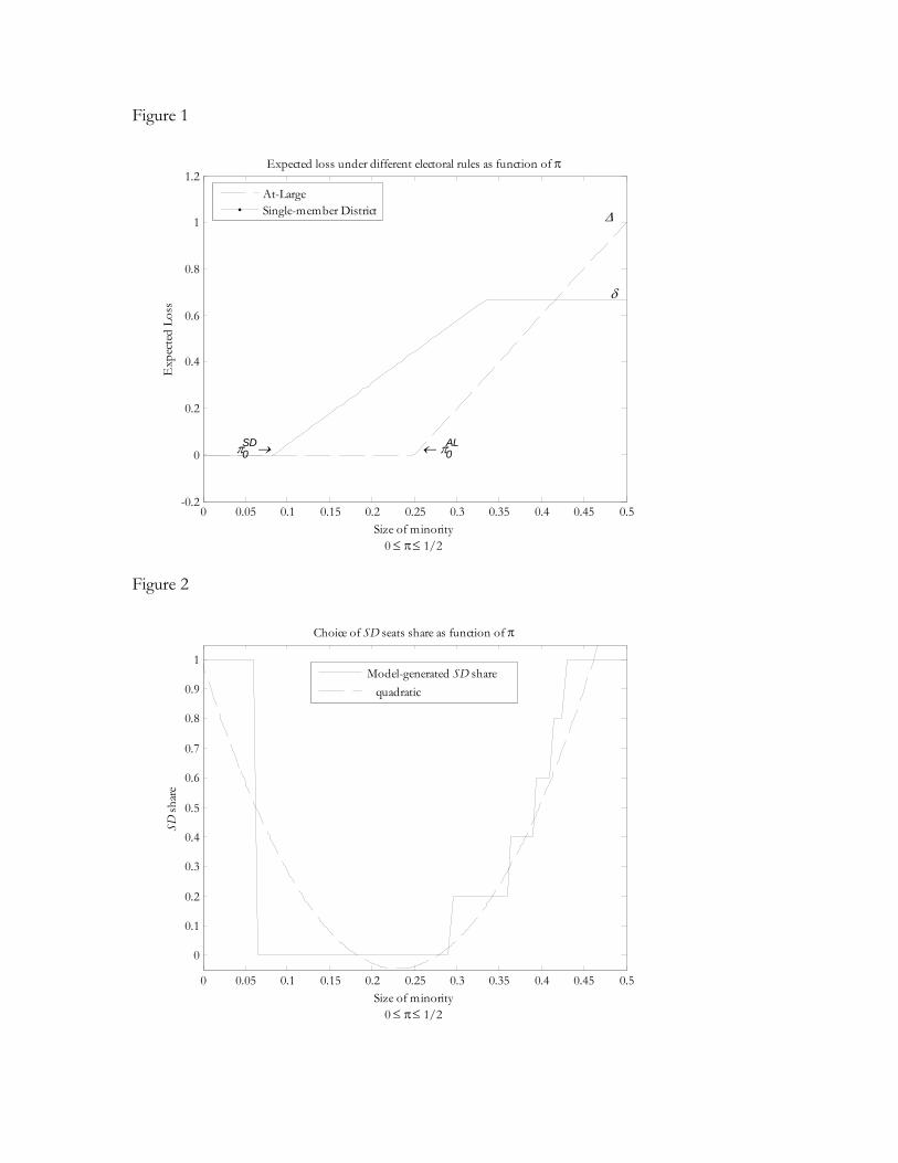
Figure 1
0 0.05 0.1 0.15 0.2 0.25 0.3 0.35 0.4 0.45 0.5-0.2
0
0.2
0.4
0.6
0.8
1
1.2
Size of minority0 ≤ π ≤ 1/2
Exp
ecte
d Lo
ssExpected loss under different electoral rules as function of π
← π0AL π0
SD→
∆
δ
At-LargeSingle-member District
Figure 2
0 0.05 0.1 0.15 0.2 0.25 0.3 0.35 0.4 0.45 0.5
0
0.1
0.2
0.3
0.4
0.5
0.6
0.7
0.8
0.9
1
Size of minority0 ≤ π ≤ 1/2
SD sh
are
Choice of SD seats share as function of π
Model-generated SD share quadratic
Figure 3
0 0.05 0.1 0.15 0.2 0.25 0.3 0.35 0.4 0.45 0.50
0.2
0.4
0.6
0.8
1
1.2
1.4
Exp
ecte
d U
tility
Expected utility under different electoral rules as function of π
Mixed systemAt-LargeSingle-member District
Size of minority0 ≤ π ≤ 1/2

Table 1Size of Minority and City Electoral Rule: Main Non-Monotonicity, All U.S.
Dependent variable: Fraction of councilmen elected by district
Sample period:Cross-section 1990
Cross-section 1990
Cross-section 1990
Panel 1970-2000
Panel 1970-2000
Panel (a)Estimator: OLS OLS 2SLS City F. E. City F. E.
(1) (2) (3) (4) (5)Frac. Minority -0.360 -0.292 -0.645 -0.622 -0.697
[0.115]*** [0.118]** [0.191]*** [0.202]*** [0.203]***(Frac. Minority)^2 0.410 0.375 1.011 1.078 1.114
[0.189]** [0.190]** [0.356]*** [0.284]*** [0.284]***Log(City Population) 0.062 0.105 0.064 0.021 -0.750
[0.007]*** [0.091] [0.008]*** [0.027] [0.229]***Log(Median Income) -0.237 -0.078 -0.253 -0.010 2.081
[0.015]*** [0.530] [0.019]*** [0.048] [0.911]**Controls Included Included
Observations 3601 3601 2491 11485 11485R-squared 0.06 0.07 0.07 0.84 0.84Minimum of U-function (π*) 0.438 0.388 0.318 0.288 0.312Observations π > π* 198 288 280 1678 1462No relation F-test (p-value) 0.002 0.041 0.002 0.000 0.000
Panel (b)
Estimator: Tobit Tobit IV Tobit Tobit R. E. Tobit R. E.
(1) (2) (3) (4) (5)Frac. Minority -2.840 -2.211 -4.353 -2.525 -2.391
[0.707]*** [0.728]*** [0.981]*** [0.252]*** [0.254]***(Frac. Minority)^2 3.230 2.831 6.301 3.118 3.108
[1.119]*** [1.135]** [1.674]*** [0.382]*** [0.384]***Log(City Population) 0.401 1.258 0.389 0.238 0.291
[0.043]*** [0.515]** [0.051]*** [0.016]*** [0.197]Log(Median Income) -1.692 14.254 -1.737 -1.030 8.317
[0.134]*** [4.990]*** [0.163]*** [0.051]*** [1.801]***Controls Included Included
Observations 3601 3601 2491 11485 11485Minimum of U-function (π*) 0.439 0.390 0.345 0.404 0.384Observations π > π* 197 276 246 848 948No relation F-test (p-value) 0.000 0.008 0.000 0.000 0.000Notes: Robust standard errors in brackets below coefficients. * significant at 10%; ** significant at 5%; *** significant at 1%. In panel (a) and (b) standard errors are clustered at the city level for columns (4) and (5). Regressions of columns (4) and (5) include year fixed effects. No relation F-test refers to the joint test for the null hypothesis that Frac. Minority and Frac. Minority squared are zero. For column (2) controls are: the squared log of city population and income, the fraction of population employed in manufacturing, agricolture, mining, trade, financial services, and fraction above 65 years of age. For column (3) the instruments set includes t-10 lags of frac. minority and its square and an indicator variable for Southern cities. For column (5) controls are the squared log of city population and income.

Table 2Pre-VRA in the South: Validation tests
Dependent variable: Fraction of councilmen elected by district
Sample period:Cross-section 1950
Cross-section 1960
Panel 1930-1960
Panel (a)Estimator: OLS OLS City F. E.
(1) (2) (3)Frac. Minority 0.308 0.226 0.406
[0.413] [0.358] [0.841](Frac. Minority)^2 -0.852 -0.478 -0.661
[0.776] [0.744] [1.322]Log(City Population) -0.045 -0.015 0.001
[0.021]** [0.017] [0.042]Log(Median Income) -0.145
[0.058]**
Observations 486 652 1482R-squared 0.01 0.02 0.81No relation F-test (p-value) 0.376 0.811 0.882
Panel (b)
Estimator: Tobit Tobit Tobit R. E.
(1) (2) (3)Frac. Minority 2.020 2.190 1.803
[3.268] [3.154] [1.061]*(Frac. Minority)^2 -5.648 -4.240 -2.832
[6.579] [6.304] [2.062]Log(City Population) -0.372 -0.147 -0.115
[0.160]** [0.155] [0.044]***Log(Median Income) -1.298
[0.514]**
Observations 486 652 1482No relation F-test (p-value) 0.566 0.784 0.180Notes: Robust standard errors in brackets below coefficients. * significant at 10%; ** significant at 5%; *** significant at 1%. In panel (a) and (b) standard errors are clustered at the city level for column (3). Regressions of column (3) include year fixed effects. No relation F-test refers to the joint test for the null hypothesis that Frac. Minority and Frac. Minority squared are zero.

Table 3Post-VRA reaction to minority enfranchisement and the selection of electoral rules in the South
before Allen v. State Board of Elections (1969)
Tabulation of changes in electoral rules 1960-67
All SouthSDshare 1960 > 0.5 (SD)
SDshare 1960 < 0.5 (AL)
VRA-Covered
SDshare 1960 > 0.5 (SD)
SDshare 1960 < 0.5 (AL)
∆(SDshare 1960-67) > 0 17 4 6 15∆(SDshare 1960-67) = 0 54 398 22 252∆(SDshare 1960-67) < 0 90 34 39 2Tot. 597 161 436 336 67 269
Dependent variable:Within-city change in the fraction of councilmen elected by district between 1960 - 1967
Sample period: 1960-67 1960-67 1960-67 1960-67 1960-67 1960-67
All SouthSDshare 1960 > 0.5 (SD)
SDshare 1960 < 0.5 (AL)
VRA-Covered
SDshare 1960 > 0.5 (SD)
SDshare 1960 < 0.5 (AL)
Estimator: First Diff. First Diff. First Diff. First Diff. First Diff. First Diff.(1) (2) (3) (4) (5) (6)
Frac. Minority 1960 -0.143 -2.335 0.433 -0.146 -2.560 0.457[0.353] [0.739]*** [0.239]* [0.363] [0.977]** [0.235]*
(Frac. Minority 1960)^2 -0.125 3.104 -0.940 -0.100 3.905 -0.911[0.775] [1.487]** [0.480]* [0.758] [1.804]** [0.457]**
∆Log(City Pop.) 1960-67 0.167 -0.027 0.138 0.194 0.548 0.151[0.075]** [0.151] [0.064]** [0.068]*** [0.474] [0.057]***
∆Log(Med. Inc.) 1960-67 -0.113 -0.301 0.034 -0.071 -0.317 0.000[0.065]* [0.156]* [0.049] [0.067] [0.237] [0.038]
No relation F-test (p-value) 0.279 0.001 0.148 0.355 0.032 0.138Observations 1551 345 1206 838 141 697R-squared 0.79 0.69 0.79 0.76 0.67 0.74Tot. No. Changers 592 332Notes: The date of the VRA is 1965. Robust standard errors in brackets below coefficients. * significant at 10%; ** significant at 5%; *** significant at 1%. Columns (1)-(3) employ sample of all Southern cities; (4)-(6) only cities in VRA-covered States. In these first difference specification frac. minority and its square enter in 1960 levels in order to proxy for the extension of the franchise to minorities.

Table 4City Electoral Rule and Minority Representation: Cross-sectional and Within-city variation
Sample: All U.S.Frac. Minority < mean( Frac. Minority )
mean( Frac. Minority ) < Frac. Minority < π*
π* < Frac. Minority
Panel (a): OLS, cross-section 1990Dependent variable: Representaional ratio
(1) (2) (3) (4)SD Share 0.082 0.081 0.146 0.088
[0.031]*** [0.038]** [0.057]** [0.059]Log(City Population) 0.072 0.036 0.051 0.053
[0.011]*** [0.018]** [0.017]*** [0.021]**Log(Median Income) -0.208 -0.092 -0.507 -0.202
[0.033]*** [0.035]*** [0.081]*** [0.073]***Frac. Minority 1.127 3.821 0.156 0.833
[0.057]*** [0.426]*** [0.239] [0.177]***
Observations 3507 2375 934 198R-squared 0.13 0.06 0.10 0.13
Panel (b): City Fixed Effects, panel 1980-2000Dependent variable: Representaional ratio
(1) (2) (3) (4)SD Share 0.216 0.027 0.433 0.296
[0.058]*** [0.102] [0.193]** [0.092]***Log(City Population) 0.087 0.188 -0.131 -0.028
[0.080] [0.115] [0.288] [0.132]Log(Median Income) -0.017 -0.043 0.269 -0.163
[0.120] [0.150] [0.518] [0.264]Frac. Minority -0.248 -0.359 -0.858 -0.272
[0.227] [1.105] [1.678] [0.472]
Observations 10252 6874 1925 1453R-squared 0.71 0.67 0.87 0.87Notes: Robust standard errors are in brackets below coefficients. * significant at 10%; ** significant at 5%; *** significant at 1%. Standard errors are clustered at the city level in Panel (b). In Panel (b) all regressions include year fixed effects and sample coverage period is 1980-2000. The representational ratio is the fraction of non-white councilmen in the council divided by the fraction of the population that is non-white.
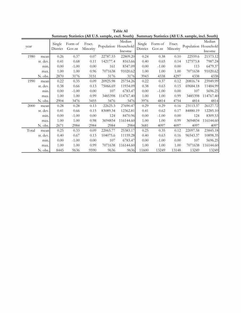
Table AISummary Statistics (All U.S. sample, excl. South) Summary Statistics (All U.S. sample, incl. South)
year Single District
Form of Gov.nt
Fract. Minority Population
Median Household
Income
Single District
Form of Gov.nt
Fract. Minority Population
Median Household
Income1980 mean 0.26 0.37 0.07 22787.53 22809.20 0.24 0.38 0.10 22559.6 21573.12
st. dev. 0.41 0.68 0.11 142177.4 8163.66 0.40 0.65 0.14 127573.8 7987.24min. 0.00 -1.00 0.00 161 8347.09 0.00 -1.00 0.00 113 6479.37max. 1.00 1.00 0.96 7071638 91020.62 1.00 1.00 1.00 7071638 91020.62
N. obs. 2870 3176 3151 3176 3176 3943 4338 4297 4338 43381990 mean 0.22 0.35 0.09 20925.98 25754.26 0.22 0.37 0.12 20816.74 23949.99
st. dev. 0.38 0.66 0.13 75066.69 11934.09 0.38 0.63 0.15 69684.18 11484.99min. 0.00 -1.00 0.00 107 6783.47 0.00 -1.00 0.00 107 5696.25max. 1.00 1.00 0.99 3485398 114767.40 1.00 1.00 0.99 3485398 114767.40
N. obs. 2904 3476 3455 3476 3476 3976 4814 4754 4814 48142000 mean 0.28 0.28 0.13 22625.3 27690.47 0.29 0.29 0.16 23113.37 26127.72
st. dev. 0.41 0.66 0.15 83089.34 12362.81 0.41 0.62 0.17 84880.19 12285.10min. 0.00 -1.00 0.00 124 8470.96 0.00 -1.00 0.00 124 8309.53max. 1.00 1.00 0.98 3694834 116144.60 1.00 1.00 0.99 3694834 116144.60
N. obs. 2671 2984 2984 2984 2984 3681 4097 4097 4097 4097Total mean 0.25 0.33 0.09 22065.77 25383.17 0.25 0.35 0.12 22097.58 23845.18
st. dev. 0.40 0.67 0.13 104075.6 11159.28 0.40 0.63 0.16 96543.37 10898.35min. 0.00 -1.00 0.00 107 6783.47 0.00 -1.00 0.00 107 5696.25max. 1.00 1.00 0.99 7071638 116144.60 1.00 1.00 1.00 7071638 116144.60
N. obs. 8445 9636 9590 9636 9636 11600 13249 13148 13249 13249

Table AIISummary Statistics: South Region
year Single District
Form of Governmen
t
Fract. Minority Population
1930 mean 0.1901865 0.6144578 0.240152 55689.73st. dev. 0.3417885 0.6756604 0.1527653 97710.1
min. 0 -1 0.00094 284.928max. 0.9473684 1 0.9616204 804874.1
N. obs. 144 166 137 1371940 mean 0.3677645 0.2313253 0.2214527 44127.13
st. dev. 0.4594916 0.7952042 0.1455125 85805.16min. 0 -1 0.0002387 4868max. 1 1 0.5976929 859100.3
N. obs. 415 415 229 2291950 mean 0.3452313 0.254065 0.2088538 32005.15
st. dev. 0.4523494 0.7459898 0.1448257 73305.76min. 0 -1 0.0001114 2774max. 1 1 0.7235112 949708.4
N. obs. 486 492 492 4921960 mean 0.2539517 0.2642643 0.1941368 34242.28
st. dev. 0.4137504 0.6755555 0.1454932 82867.91min. 0 -1 0 3202.001max. 1 1 0.6946776 939023.6
N. obs. 656 666 663 6631970 mean 0.1613318 0.2837259 0.1779699 29274.97
st. dev. 0.3543261 0.5554105 0.150278 79091.1min. 0 -1 0 2406max. 1 1 0.7703364 1199388
N. obs. 904 934 936 9361980 mean 0.1721898 0.4061962 0.1825356 21936.64
st. dev. 0.3517008 0.536582 0.1646552 74266.77min. 0 -1 0 113max. 1 1 0.9988168 1595138
N. obs. 1073 1162 1146 11621990 mean 0.2301296 0.3983558 0.2088375 20532.95
st. dev. 0.3838137 0.5150512 0.1756844 53238.92min. 0 -1 0 243max. 1 1 0.9864677 935926.6
N. obs. 1072 1338 1299 13382000 mean 0.318919 0.3225517 0.2462236 24421.92
st. dev. 0.4229846 0.5082095 0.1855629 89530.48min. 0 -1 0 138max. 1 1 0.9933691 1954847
N. obs. 1010 1113 1113 1113Total mean 0.2454504 0.3385301 0.2055153 26973.67
st. dev. 0.4016687 0.5937366 0.1662955 76418.88min. 0 -1 0 113max. 1 1 0.9988168 1954847
N. obs. 5760 6286 6015 6070