CHIRPLET SIGANL DECOMPOSITION OF ULTRASONIC SIGNAL...

CHIRPLET SIGANL DECOMPOSITION OF ULTRASONIC SIGNAL:

ANALYSIS, ALGORITHMS AND APPLICATIONS

BY

YUFENG LU

Submitted in partial fulfillment of the requirements for the degree of

Doctor in Philosophy in Electrical Engineering in the Graduate College of the Illinois Institute of Technology

Approved _________________________ Adviser

Chicago, Illinois May 2007

iii

ACKNOWLEDGEMENT

I would like to express my sincere gratitude and appreciation to my advisor, Dr.

Jafar Saniie, for his encouragement, motivation, inspiration, guidance and friendship

throughout all phases of my Ph.D study at Illinois Institute of Technology. I am very

grateful to my defense committee members: Dr. Guillermo E. Atkin, Dr. Erdal Oruklu,

and Dr. Xiangyang Li, for their valuable comments and suggestion on this work. I am

also thankful to my colleagues and friends: Dr. Ramazan Demirli, Dr. Guillerme

Cardoso, Dr. Fernando Martinez Vallina, and Mr. Logan Sorenson, in particular, to

Ramazan and Guillerme for their valuable discussion to enhance the work, to Logan for

the collaboration in the hardware implementation chapter.

I would like to dedicate the work to my family: my wife, my parents, and my

sister. This work would not be possible without their years of constant support,

encouragement and love. The special thanks to my wife, Jie Jiao for the endless patience

and understanding. The work witnesses the days from China to United States, from

Syracuse to Chicago.

iv

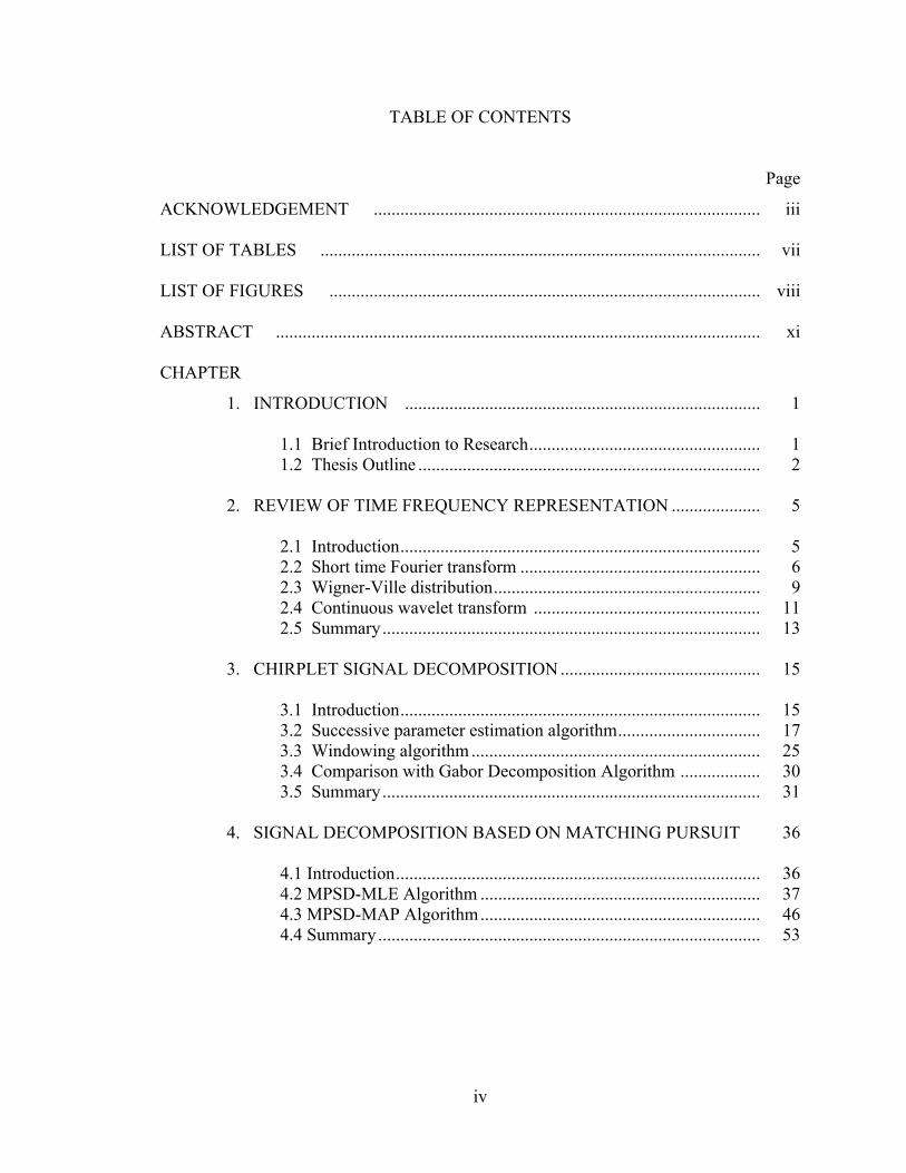
TABLE OF CONTENTS

Page

ACKNOWLEDGEMENT ....................................................................................... iii

LIST OF TABLES ................................................................................................... vii

LIST OF FIGURES ................................................................................................. viii

ABSTRACT ............................................................................................................. xi

CHAPTER

1. INTRODUCTION ................................................................................ 1

1.1 Brief Introduction to Research .................................................... 1 1.2 Thesis Outline ............................................................................. 2

2. REVIEW OF TIME FREQUENCY REPRESENTATION .................... 5

2.1 Introduction ................................................................................. 5 2.2 Short time Fourier transform ...................................................... 6 2.3 Wigner-Ville distribution ............................................................ 9 2.4 Continuous wavelet transform ................................................... 11 2.5 Summary ..................................................................................... 13

3. CHIRPLET SIGNAL DECOMPOSITION ............................................. 15

3.1 Introduction ................................................................................. 15 3.2 Successive parameter estimation algorithm ................................ 17 3.3 Windowing algorithm ................................................................. 25 3.4 Comparison with Gabor Decomposition Algorithm .................. 30 3.5 Summary ..................................................................................... 31

4. SIGNAL DECOMPOSITION BASED ON MATCHING PURSUIT 36

4.1 Introduction .................................................................................. 36 4.2 MPSD-MLE Algorithm ............................................................... 37 4.3 MPSD-MAP Algorithm ............................................................... 46 4.4 Summary ...................................................................................... 53

v

5. COMPARITIVE STUDY OF CTSD AND MPSD ALGORITHMS ...... 54

5.1 Introduction ................................................................................. 54 5.2 Derivation of Cramer-Rao Lower Bounds .................................. 55 5.3 Monte Carlo Simulation .............................................................. 59 5.4 Observation and Analysis ........................................................... 60 5.5 Summary ..................................................................................... 61

6. TARGET DETECTION OF ULTRASONIC BACKSCATTERED

SIGNAL .................................................................................................. 64

6.1 Introduction ................................................................................. 64 6.2 Real Time Ultrasonic Measurement System .............................. 64 6.3 Target Detection in Ultrasonic Backscattered Signal ................. 67 6.4 Bat Chirp Signal Analysis ........................................................... 75 6.5 Summary ..................................................................................... 76

7. STATISTICAL EVALUATION USING ULTRASONIC GRAIN

SIGNAL ................................................................................................... 83

7.1 Introduction ................................................................................. 83 7.2 Ultrasonic Backscattered Model ................................................ 84 7.3 Grain Size Evaluation Using Ultrasonic Backscattered Echoes ........................................................................................ 87 7.4 Summary ..................................................................................... 93

8. ULTRASONIC REVERBERANT APPLICATION ............................... 94

8.1 Introduction ................................................................................. 94 8.2 Reverberant Signal Model for Multilayered Structures ............. 95 8.3 Experimental Reverberant Signal Analysis ................................ 101 8.4 Summary ..................................................................................... 108

9. EMBEDDED SIGNAL DECOMPOSITION SYSTEM

IMPLEMENTATION... ........................................................................... 109

9.1 Introduction ................................................................................. 109 9.2 Embedded DSP System Based on Xilinx Virtex II Pro FPGA. . 110 9.3 Summary ..................................................................................... 114

vi

10. CONCLUSION ....................................................................................... 116

BIBLIOGRAPHY .................................................................................................... 120

vii

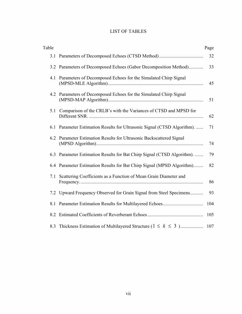
LIST OF TABLES

Table Page

3.1 Parameters of Decomposed Echoes (CTSD Method) ..................................... 32 3.2 Parameters of Decomposed Echoes (Gabor Decomposition Method) ............ 33 4.1 Parameters of Decomposed Echoes for the Simulated Chirp Signal (MPSD-MLE Algorithm) ................................................................................ 45 4.2 Parameters of Decomposed Echoes for the Simulated Chirp Signal (MPSD-MAP Algorithm) ................................................................................ 51 5.1 Comparison of the CRLB’s with the Variances of CTSD and MPSD for Different SNR. ................................................................................................ 62 6.1 Parameter Estimation Results for Ultrasonic Signal (CTSD Algorithm). ...... 71 6.2 Parameter Estimation Results for Ultrasonic Backscattered Signal (MPSD Algorithm). ......................................................................................... 74 6.3 Parameter Estimation Results for Bat Chirp Signal (CTSD Algorithm). ....... 79 6.4 Parameter Estimation Results for Bat Chirp Signal (MPSD Algorithm). ....... 82 7.1 Scattering Coefficients as a Function of Mean Grain Diameter and Frequency. ....................................................................................................... 86 7.2 Upward Frequency Observed for Grain Signal from Steel Specimens. .......... 93 8.1 Parameter Estimation Results for Multilayered Echoes .................................. 104 8.2 Estimated Coefficients of Reverberant Echoes ............................................... 105 8.3 Thickness Estimation of Multilayered Structure ( 31 ≤≤ k ) ................... 107

viii

LIST OF FIGURES

Figure Page

2.1 Comparisons of Time Frequency Techniques. a) a Simulated Signal. b) WVD of the Signal. c) STFT of the Signal (Using Hamming Window). d) CWT of the Signal (Using Morlet Wavelet). ............................................ 14

3.1 The Flowchart of CTSD Algorithm ................................................................ 28 3.2 Basic Illustration of Dominant Echo Windowing Method. a) CT of Three Interfering Chirp Echoes. b) Projection in Frequency Domain and the Frequency Window Boundary Points (Dashed Lines). c) Projection in Time Domain and the Time Window Boundary Points (Dashed Lines) ................. 29 3.3 Simulated Ultrasonic Highly Overlapping Echoes(Solid Line), Superimposed

with the Reconstructed Signals by CTSD Algorithm and Gabor Decomposition Method. ........................................................................................................... 34

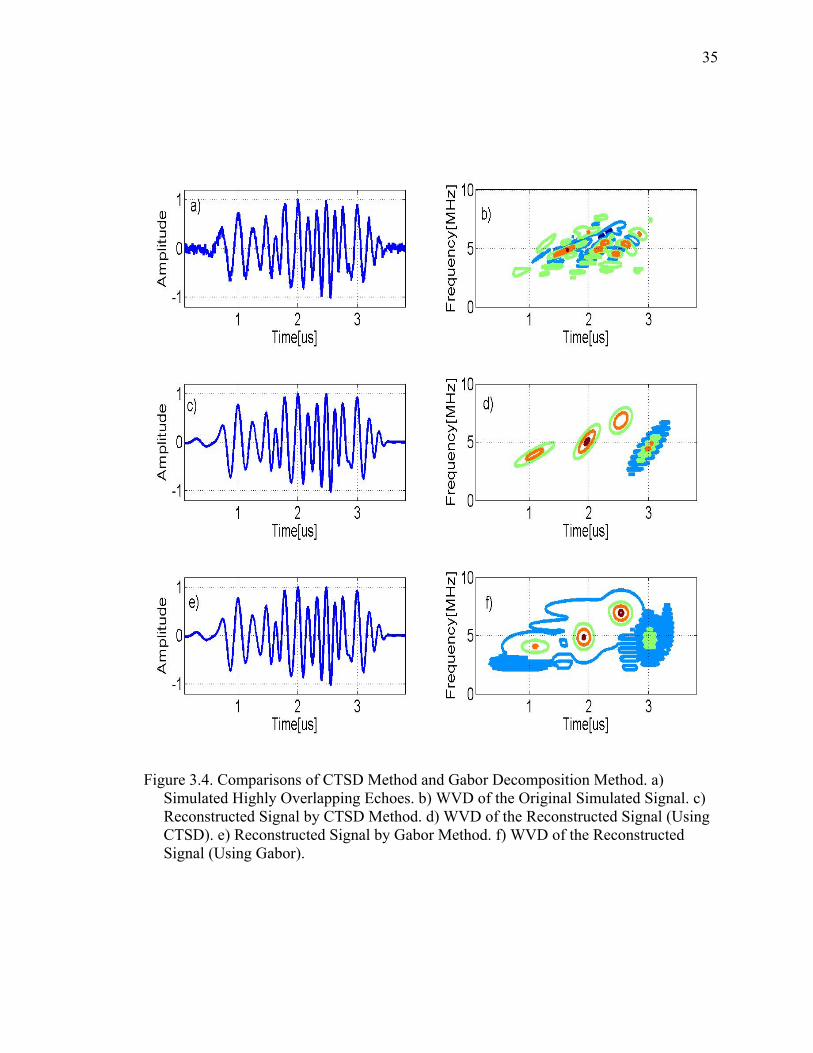
3.4 Comparisons of CTSD Method and Gabor Decomposition Method. a) Simulated

Highly Overlapping Echoes. b) WVD of the Original Simulated Signal. c) Reconstructed Signal by CTSD Method. d) WVD of the Reconstructed Signal (Using CTSD). e) Reconstructed Signal by Gabor Method. f) WVD of the Reconstructed Signal (Using Gabor)... ........................................................... 35

4.1 The Flowchart of MPSD Algorithm. .............................................................. 42 4.2 Overlapping Chirp Signal Superimposed with the Reconstructed Signal Using

MPSD-MLE Algorithm. ................................................................................. 43 4.3 a) Overlapping Chirp Signal. b) WVD of the Overlapping Chirp Signal. c) the Estimated Signal Using MPSD-MLE Algorithm. d) WVD of the Estimated Signal. ............................................................................................................. 44 4.4 Overlapping Chirp Signal Superimposed with the Reconstructed Signal Using

MPSD-MAP Algorithm. ................................................................................. 49 4.5 a) Overlapping Chirp Signal. b) WVD of the Overlapping Chirp Signal. c) the Estimated Signal Using MPSD-MAP Algorithm. d) WVD of the Estimated Signal. ............................................................................................................. 50 5.1 a) Input SNR vs. Output SNR for a Single Noisy Chirp Echo Using CTSD Algorithm. b) Input SNR vs. Output SNR for a Single Noisy Chirp Echo Using MPSD Algorithm. ............................................................................................ 62 6.1 Real Time Ultrasonic Measurement System. .................................................. 66

ix

6.2 Ultrasonic Backscattering Signal Superimposed with the Reconstructed Signal (CTSD Algorithm) ............................................................................... 67 6.3 a) Ultrasonic Backscattering Signal. b) TF representation of the Ultrasonic Backscattering Signal. c) Estimated Signal Using CTSD Algorithm. d) TF Representation of the Estimated Signal. ......................................................... 70 6.4 Ultrasonic Backscattering Signal Superimposed with the Reconstructed Signal (MPSD Algorithm) .............................................................................. 72 6.5 a) Ultrasonic Backscattering Signal. b) WVD of Ultrasonic Backscattering Signal. c) the Reconstructed Signal. d) WVD of the Reconstructed Signal Using MPSD Algorithm. ................................................................................ 73 6.6 Experimental Bat Chirp Signal Superimposed with the Estimated Result (CTSD Algorithm). ......................................................................................... 77 6.7 a) Experimental Bat Chirp Signal. b) TF Representation of the Experimental Bat Chirp Signal. c) Estimated Signal. d) TF Representation of the Estimated Signal. .............................................................................................................. 78 6.8 Experimental Bat Chirp Signal Superimposed with the Estimated Result (MPSD Algorithm). ......................................................................................... 80 6.9 a) Experimental Bat Chirp Signal. b) WVD of Bat Chirp Signal. c) the

Reconstructed Signal. d) WVD of the Reconstructed Signal Using MPSD Algorithm. ...................................................................................................... . 81

7.1 Microscopes of Specimens. a) Steel-ref. b) Steel-1600. c) Steel-1900. .......... 89 7.2 Grain Signals of Steel Specimens. (I) Shows Grain Signal. (II) Shows Magnitude Spectrum. a) Steel-ref. b) Steel-1600. c) Stell-1900. .................... 91 8.1 Reverberation Path in Signal Thin Layer. ....................................................... 96 8.2 Multilayered Structures Consisting of Four Different Regions. ..................... 97 8.3 Variation of Wave Paths with Equivalent Traveling Time for Case Where k=2 and L=2. ................................................................................................... 98 8.4 The Reconstructed Reverberant Echoes Superimposed with the Experimental Reverberant Echoes of Multilayered Structure. .............................................. 103 8.5 Comparison of Envelope of Class “a” Echoes, “b” Echoes and “c” Echoes. . 106

x

9.1 Architecture Overview of Embedded FPGA-Based System........................... 113 9.2 Process Experimental Ultrasonic Echoes on FPGA-Based DSP System ....... 115

xi

ABSTRACT

A major and challenging problem in ultrasonic nondestructive evaluation (NDE)

is the ultrasonic backscattered signal analysis in presence of high scattering noise. The

pattern of Ultrasonic backscattered signal represents the shape, size and orientation of

ultrasonic reflectors and the physical property of propagation path. The signal loss by the

effect of scattering and absorption imposes a limit on the detection capability of

ultrasonic NDE systems. Therefore, signal modeling and parameter estimation of the

nonstationary ultrasonic signal is critical for precise evaluation of objects.

Joint time-frequency signal representation is an important method to evaluate the

nonstationary characteristic of ultrasonic backscattered signal. It can be shown that the

conventional time frequency transform such as Wigner Ville Distribution and Short time

Fourier transform introduce cross-terms , offer poor resolution, and are sensitive to noise

level. On the other hand, the continuous wavelet transform shows higher time resolution

in smaller scale and higher frequency resolution in high scale. This is a preferable

property for tracking the time-varying frequency of nonstationary signal, especially in

ultrasonic model based algorithm design.

In this study, we introduced chirplet transform (CT) as a means not only to obtain

time frequency representation of signal, but also to be utilized for chirplet signal

decomposition and successive parameter estimation. Based on the assumption that the

signal to be processed, no matter how complex, can be decomposed into superimposition

of multiple chirplet echoes, the chirplet signal decomposition based on chirplet transform

(CTSD) algorithm is developed. It utilizes the chirplet transform of signal to locate the

most dominant chirplet component and successively estimate its parameters, such as

xii

time-of-arrival, center frequency, chirp rate, phase and intensity. Compared with signal

decomposition based on Gabor function, the chirplet signal decomposition algorithm is

very effective in representing dispersive ultrasonic echoes due to the parameter diversity

of chirplets. Analysis and simulation results show that the performance of chirplet signal

decomposition overwhelms that of the Gabor decomposition with less number of

components to reconstruct the same high overlapping signal.

As an alternative, we developed matching pursuit signal decomposition(MPSD)

algorithm through incorporating statistical methods such as Maximum Likelihood

Estimation (MLE) and Maximum a Posteriori (MAP) into a general nonstationary signal

analysis frame work (i.e., matching pursuit algorithm). The MPSD algorithm iteratively

optimizes the parameters of a chirplet function to match the signal and achieve high

resolution decomposition. This approach avoids the exhaustive search of a large number

of dictionary functions and leads to a more efficient implementation.

Furthermore, we derived analytical Cramer Rao Lower Bound (CRLB) of chriplet

estimator. The performance of CTSD and MPSD algorithm are evaluated against the

CRLB bounds. Computer simulation indicates noise is better suppressed in CTSD

algorithm than it is in MPSD algorithm. Monte Carlo analysis shows that both algorithms

are minimum variance unbiased (MVU) estimators, hence they provide optimal

parameter estimation and robust chirplet signal decomposition.

We also explored different applications of the chirplet signal decomposition

approaches. The estimated parameters from the experimental signals have been

successfully used to locate the target echo in ultrasonic reverberant signal, evaluate grain

size of materials, and classify ultrasonic multilayered reverberant echoes. Moreover, an

xiii

embedded hardware system is implemented on Xilinx Virtex II Pro FPGA platform to

accelerate the chirplet signal decomposition algorithm. Through computer simulation and

analysis of experimental signals, this type of study addresses a broad range applications

including target detection, deconvolution, object classification, velocity measurement,

and ranging system.

1

CHAPTER 1

INTRODUCTION

1.1 Brief Introduction to Research

Ultrasonic waves have been applied in testing and imaging of material for a long

time. In the ultrasonic pulse-echo testing, ultrasonic signal travels through medium

without changing their physical states. The signal undergoes an energy loss due to

absorption and scattering of the internal microstructure on the propagation path. Hence,

the information of microstructure is inherent to the measured backscattered ultrasonic

signal. It can be utilized to characterize the propagation path which determines the

physical properties of reflectors, in terms of their location, geometric shape, size,

orientation and microstructure. Through the signal analysis, the useful feature of the

medium can be extracted. This is the property that supports the broad applications of

ultrasound in non-destructive evaluation (NDE) of material, and medical diagnosis.

The extraction of the desired information related to the properties of the medium

requires models to simulate the formation of echoes. From system point of view, the

measured backscattered signal can be simplified as the convolution result of input signal

(i.e., the transducer excitation pulse) and system response. The parameters of the

backscattered echoes such as time-of-arrival, center frequency, amplitude, bandwidth,

phase, and chirp rate are of important for their significance to dissolve the system

response. For example, the time-of-arrival and amplitude of the echo can be attributed to

the target response in term of target location, size and orientation. The variation of time-

of-arrival and amplitude can be attributed to the energy loss and the traversed time. The

center frequency, bandwidth and the phase of the echo can be attributed to the frequency

2

modification of the propagation path (i.e. characterization of media impedance). The

chirp rate can be attributed to the dispersion phenomenon in the traveling of ultrasonic

wave.

In this research, to form an efficient way to model the ultrasonic backscattered

echoes, we propose chirplet signal decomposition algorithm based on the chirplet

transform. The mathematical foundation of the algorithm is discussed. Another

decomposition implementation scheme which is based on the matching pursuit

framework is compared and discussed. The analytical Cramer-Rao bounds of the

algorithms are explored and compared with the simulated results. Furthermore, the

proposed algorithm is tested and verified in the different applications such as target

detection, bat chirp signal analysis, material grain size evaluation, and multilayered

structure inspection. Furthermore, an embedded FPGA-based DSP system for signal

decomposition is analyzed.

1.2 Thesis Outline

Chapter 2 presents a brief review concerning time frequency representation. Three

notably used time frequency representations such as short time Fourier transform,

Wigner-Ville distribution, and continuous wavelet transform are outlined. The time

resolution and frequency resolution of the three time frequency representations are

discussed.

Chapter 3 lays out the mathematical foundation of chirplet signal decomposition.

The basic idea behind the chirplet signal decomposition is to decompose any complex

signal into a linear combination of chirplet model and estimate all the parameters of the

3

model precisely. First, the chirp signal and its application background are presented.

Then, the successive parameter estimation algorithm based on chirplet transform is

elaborately derived with mathematical details. Furthermore, a windowing strategy is

applied in both time domain and frequency domain to generalize the successive

parameter estimation algorithm to decompose multiple high overlapping signals. In order

to demonstrate the robustness of chirplet model and the efficiency of chirplet signal

decomposition algorithm, we simulate a signal with multiple highly-overlapping echoes.

The simulated signal is examined by the chirplet signal decomposition algorithm and

another decomposition algorithm from the literature, which is based on Gabor function.

The performances of these two algorithms are compared with each other and discussed

with details.

Alternatively, Chapter 4 introduces signal decomposition based on matching

pursuit (MPSD) framework. The matching pursuit framework was proposed by Mallat et.

al for non-stationary signal analysis. In the original matching pursuit algorithm, it uses

correlation criteria to search the best matching function in dictionaries. It has been

reported that this criterion obtains decompositions adaptive to global signal

characteristics. Since in some applications, it is preferable to be best adapted to the local

structures of signal, we incorporate the statistical analysis tools such as Maximum

Likelihood Estimation and Maximum a Posteriori into the implementation of

decomposition. The implementation details of the algorithms and simulation results are

discussed in Chapter 4. To benchmark the proposed signal decomposition algorithms,

Chapter 5 explores the analytical lower bound, i.e., the Cramer-Rao lower bound (CRLB).

4

We evaluate the performance of the signal decomposition and parameter estimation

algorithms against the analytical CRLB bounds through Monte Carlo simulation.

Chapter 6 presents the applications of the chirplet signal decomposition algorithm

and the signal decomposition based on matching pursuit in ultrasonic target detection and

bat chirp signal analysis. Chapter 7 introduces the application of material grain size

evaluation. The chirplet signal decomposition algorithm is applied to estimate the grain

size of materials which are processed under different heat treatment condition. As another

important aspect of ultrasonic nondestructive evaluation, Chapter 8 lay out the discussion

of the multilayered reverberant structures. The proposed algorithm is evaluated by

ultrasonic multilayered reverberant echoes. To verify the feasibility of hardware

implementation and acceleration of the algorithm, In Chapter 9, an embedded hardware

design of signal decomposition algorithm is analyzed and implemented on Xilinx Virtex

II Pro Field Programmable Gate Array (FPGA) Platform. Finally, Chapter 10 summaries

the research of chirplet signal decomposition algorithm and its applications.

5

CHAPTER 2

REVIEW OF TIME-FREQUENCY REPRESENTATION

2.1 Introduction

In this chapter, the background of time-frequency representation is reviewed.

Then three commonly used methods of time-frequency signal representation such as short

time Fourier transform, Wigner Ville distribution and continuous wavelet transform are

introduced. The time resolution and frequency resolution are discussed and compared

among the three time frequency representations.

The need for time-frequency representation is from the nonstationary nature of

most signals in real world. Usually it is inadequate to fully describe the signal using

either time domain or frequency domain analysis. Time-frequency representation is a

useful tool for simultaneous characterization of a signal in time and frequency domain. It

provides information about how the spectrum of the signal changes with time, thus

leading to accurately describe, analyze and interpret the nonstationary signal. The time-

frequency process is performed by mapping the signal from time domain, where the

signal is one-dimensional, into a two dimensional expression (i.e., time frequency

domain). A variety of methods for obtaining time frequency representation have been

devised, most notably the short time Fourier transform (STFT), the Wigner-Ville

distribution (WVD) and the continuous wavelet transform.

6

2.2 Short Time Fourier Transform (STFT)

During the 1940s, the motivation to analyze the human speech, which is

nonstationary and rapidly varying spectral components, led to the invention of sound

spectrogram (i.e., STFT). In order to analyze such a non-stationary signal, it is

reasonable to apply a small window along time axis in order to examine the frequency

content of the signal in the given time window. The STFT aims to obtain the short time

Fourier transform of a signal by sliding a time window and then taking the Fourier

transform of the windowed signal. In doing so, it is assumed that the signal is stationary

during the duration of the time window. The STFT of a signal can be expressed as:

( ) ∫+∞

∞−

−−= dtettgtftSTFT tif

0)()(, 000ωω (2.1)

Here, )( tg is a normalized real and symmetric window

)()( tgtg −= , 1)( =tg (2.2)

Using different type windows result in different TF representations. Since there

already have extensive research efforts in the classic signal processing field, such as

efficient implementation of Fourier transform, correlation and filter design theory in past

years, they can be imported into the implementation of STFT.

The downfall of STFT is from the windowing process, which leads to inherent

trade off between time resolution and frequency resolution. The resolution problem of

STFT can be revealed by the following expression of time spread tσ and frequency

spread ωσ of the window function )( tg .

Let )(ˆ ωg denote ))(( tgFT , then from properties of Fourier transform,

7

( ) ))((ˆ 0)(

000 ttgFTeg it −=− −− ωωωω (2.3)

Hence, the time spread tσ and frequency spread ωσ are

( ) ( )

( )∫∫

∞+

∞−

+∞

∞−

−

=

−−=

dttgt

dtettgtt tit

22

2

02

02 0ωσ

(2.4)

( ) ( )

( )∫

∫∞+

∞−

+∞

∞−

=

−−=

ωωωπ

ωωωωωπ

σ ωω

dg

deg ti

22

2

02

02

ˆ21

ˆ21

0

(2.5)

From Equation 2.4 and Equation 2.5, it can be seen that the spreads are independent of

the time shift, 0t , and the frequency shift, 0ω . Therefore, STFT has the same time

resolution and the same frequency resolution across time frequency plane. Can the time

resolution and the frequency resolution of STFT both be arbitrarily small to reveal the

non-stationary property of signal? Unfortunately, Heisenberg uncertain principle limits

the scheme.

Heisenberg uncertainty principle [Mal99] expresses a fundamental relationship

between the time spread and the frequency spread of the windowed signal. It states the

mathematical fact that a narrow waveform yields a wide spectrum and a wide waveform

yields a narrow spectrum. Both the time waveform and the frequency spectrum can not

be made arbitrarily small simultaneously.

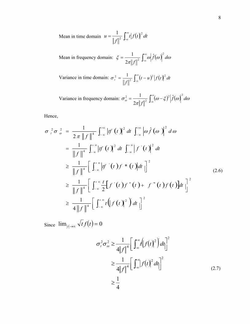
The Heisenberg uncertain principle can be derived as following. Given a

signal ( ) ( )RLtf 2∈ , the mean and variance of signal in time domain and frequency

domain can be expressed as following.

8

Mean in time domain ( )∫+∞

∞−= dttft

fu 2

2

1

Mean in frequency domain: ( )∫+∞

∞−= ωωω

πξ df

f

2

2ˆ

21

Variance in time domain: ( ) ( )∫+∞

∞−−= dttfut

ft

222

2 1σ

Variance in frequency domain: ( ) ( )∫+∞

∞−−= ωωξω

πσω df

f

222

2 ˆ2

1

Hence,

( ) ( )

( ) ( )

( ) ( )

( ) ( ) ( ) ( )[ ]

( )( ) 2'2

4

2'**'

4

2'

4

2'2

4

22

422

41

21

*1

1

ˆ2

1

⎥⎦⎤

⎢⎣⎡≥

⎥⎦⎤

⎢⎣⎡ +≥

⎥⎦⎤

⎢⎣⎡≥

=

=

∫

∫

∫

∫∫

∫∫

∞+

∞−

∞+

∞−

∞+

∞−

∞+

∞−

∞+

∞−

+∞

∞−

+∞

∞−

dttftf

dttftftftftf

dttfttff

dttfdtttff

dfdtttff

t ωωωπ

σσ ω

(2.6)

Since ( ) 0lim =∞→ tftt

( )( )

( )

414

1

41

22

4

2'24

22

≥

⎥⎦⎤

⎢⎣⎡≥

⎥⎦⎤

⎢⎣⎡≥

∫

∫∞+

∞−

∞+

∞−

dttff

dttftf

t ωσσ

(2.7)

9

The principle shows that there is a lower bound of ωσσ t .

Through the above discussion of time resolution and frequency resolution, it can

be seen that in STFT, the resolutions solely depend on the resolution property of the short

time window. The inherent lower bound of Heisenberg principle determines the tradeoff

between time resolution and frequency resolution of STFT. For a non-stationary signal,

it is always problematic to find an appropriate type and size of the window to fit the

specific signal analysis in STFT of signal. To demonstrate the STFT of a signal, Figure

2.1a shows a simulated ultrasonic signal consisting of two chirp echoes. Figure 2.1c

shows the STFT of the signal in Figure 2.1a using Hamming window.

2.3 Wigner-Ville Distribution (WVD)

Another well-known time frequency representation, Wigner-Ville Distribution

(WVD), has been received research attention for many years. In 1932, Wigner presented

a joint probability function for the coordinates and moment in the study of statistical

quantum mechanics [Wig32]. Ville derived the Wigner distribution for analytic signals

in 1948, which is known as Wigner-Ville distribution (WVD) [Vil48]. In 1946, Gabor

presented the method to expand the given signal into a sum of elementary signals of

“minimum” spread in time and frequency [Gab46]. In 1966, Cohen generalized time-

frequency representation into different distribution functions [Coh89].

A great interest was shown in time-frequency analysis in the 1980’s when a large

number of researchers started exploring the field of time frequency representation in

signal processing area [Coh89]. In the implementation of discrete Wigner-Ville

distribution, Classsen discussed the sampling rate to avoid aliasing [Cla80]. Boualem

10

Boashash et. al made a significant contribution towards Wigner-Ville analysis of time

varying signals, non-stationary random signals, cross spectral analysis, estimation and

interpretation of instantaneous frequency[Boa03].

The WVD of signal can be expressed as

∫∞+

∞−

−⎟⎠⎞

⎜⎝⎛ −⎟

⎠⎞

⎜⎝⎛ += τττω τω detftftWVD i

f0

22),( 0

*000 (2.8)

From the analysis of STFT in Section 2.2, it can be seen that the time and

frequency resolution is limited by the resolution of correlated window ( )tg in STFT. But

in WVD representation of signal, it is calculated by correlating the signal with a time and

frequency translation of the signal. From Equation 2.8, it can be seen that the time

resolution and frequency resolution are solely determined by the signal ( )tf itself.

Hence the WVD representation does not have the resolution loss from windowing.

Although WVD has excellent time and frequency resolution, the quadratic

property of WVD is that the cross terms (i.e., artifacts) are introduced when dealing with

multi-component signals. The artifacts lead to an erroneous interpretation of the time

frequency representation of the signal. The cross terms indicate that the time-frequency

energy is distributed to the place where the signal doest not really exist on the joint time-

frequency domain. To demonstrate the cross terms problem of WVD representation in

the case of multi-component signal, an example is demonstrated in the Figure 2.1. Figure

2.1a is the simulated multi-component signal. Figure 2.1b clearly shows the cross term

between these two components of the signal.

Many researchers worked on the problem of cross-terms in WVD by smoothing,

windowing, interpolating, filtering in time domain, frequency domain, or joint time-

11

frequency domain so that to attenuate the cross terms [And87, Gre96, and Oeh97].

Usually, the suppression and elimination of the cross-terms is achieved at the cost of

marginal properties and computation.

2.4 Continuous Wavelet Transform (CWT)

In the STFT implementation, a window is designed to slide along the time axis.

Once the window is chosen, the time resolution and the frequency resolution are fixed. In

certain applications, it is more desirable to have better time resolution at higher

frequencies than that at lower frequency. As a result of this characteristic, wavelet

transform have become a useful tool for non-stationary signal analysis. Since wavelet

theory were developed independently in multiple fields such as mathematics, quantum

physics, and electrical engineering, it is difficult to track a unique origin of wavelet

theory.

In 1984, Grossman and Morlet broadly defined wavelets in the context of

quantum physics. They discussed decomposition of hardy functions into square

integrable wavelets of constant shape [Gro84]. In 1985, Stephane Mallet gave wavelets

an ice-break jump through his work in digital signal processing [Mal89, Mal99]. For the

first time, he discovered some relationship between quadrature mirror filters, pyramidal

algorithm, and orthonormal wavelet bases. After that, many researchers such as Meyer,

Ingrid Daubechies worked out many sets of wavelets [Dau92, Mey93].The continuous

wavelet transform, discrete wavelet transform, and the fast implementation of wavelet

transform have been extensively explored by researchers. The wavelets have been

applied to a broad range of applications such as denoising, compression, spectral

12

estimation, pattern recognition, human vision, radar and sonar etc [Dau90, Mal91, Ant92,

Rod98, Zen01, and Cha06]. Wavelet becomes a general mathematical tool in the similar

way as the Fourier transform does. Nevertheless, we are not going to discuss the discrete

wavelet transform and the details of different wavelet base functions. We focus on the

similar resolution argument in the introduction of continuous wavelet transform as the

discussion in the STFT and WVD section. Unlike STFT and WVD, continuous wavelet

transform (CWT), through the correlation of the signal with a scaling and translating

function of wavelet ( )tψ , has varying resolution at different scale. The role of scale acts

as the role of frequency in WVD and STFT.

The CWT of signal ( )tf can be expressed as

( )

( ) ( )∫

∫∞+

∞−

∞+

∞−

=

⎟⎠⎞

⎜⎝⎛ −

=

ωωψπ

ψ

ω desstf

dtstt

stfstCWT

ti 0*

0*0

ˆˆ21

1),(

(2.9)

Here ( )tψ satisfies ( )∫+∞

∞−=0dttψ and ( )ωψ̂ denotes ( )( )tFT ψ .

0t denotes the center time of ( )tψ

0ω denotes the center frequency of ( )ωψ̂

tσ denotes the time spread of ( )tψ

ωσ denotes the frequency spread of ( )ωψ̂

Then the time spread of ⎟⎠⎞

⎜⎝⎛ −

stt

s01 ψ is

13

( ) ( ) 222222

0*20

1tsdtttsdt

stt

stt σψψ ==⎟

⎠⎞

⎜⎝⎛ −

− ∫∫∞+

∞−

∞+

∞− (2.10)

and the frequency spread of ( ) 0*ˆ tiess ωωψ is

( )( ) ( )

2

2

20

220

0

2*2

0ˆ

21

ˆ21

ss

ddss

sωσ

ωωψωωπωωψωω

π=

−=⎟

⎠⎞

⎜⎝⎛ −

∫∫

+∞

∞+

(2.11)

Hence the wavelet window ⎟⎠⎞

⎜⎝⎛ −

stt

s01 ψ centered at ⎟

⎠⎞

⎜⎝⎛

st 0

0 , ω in time frequency domain

and the time spread is tsσ , frequency spread issωσ . And the product ωσσ t still keeps

unchanged, which is the inherent property of Heisenberg uncertain principle. It is worth

to point out that the time resolution and frequency resolution depend on the scale s . This

shows higher time resolution in smaller scale and higher frequency resolution in higher

scale. As a comparison, the CWT using morlet wavelet is shown in Figure 2.1d.

2.5 Summary

In this chapter, we reviewed the time frequency representation of signal and

introduced three conventional time frequency representations such as short time Fourier

transform, Wigner-Ville distribution, and continuous wavelet transform. From all the

preliminary analysis, it can be seen that the conventional time frequency representation

such as WVD and STFT introduce cross terms, have poor resolution and are sensitive to

noise level. On the other hand, CWT shows higher time resolution in smaller scale and

higher frequency resolution in higher scale. Hence, it is a preferable property for tracking

14

the time-varying frequency of non-stationary signals, especially in our ultrasonic model

base algorithm design.

Figure 2.1 Comparisons of Time Frequency Techniques. a) a Simulated Signal. b) WVD of the Signal. c) STFT of the Signal (using Hamming Window) d) CWT of the Signal (Using Morlet Wavelet).

15

CHAPTER 3

CHIRPLET SIGNAL DECOMPOSITION

3.1 Introduction

It has been reported [San89, Wan91, and San94] that the broadband ultrasonic

backscattered signal depicts a downward shift in frequency due to signal attenuation. It

means that the higher frequencies are experienced more attenuation than the lower

frequencies. On the other hand, in the Rayleigh region of scattering, an upward trend in

frequency due to scattering is experienced. This implies that the high frequency

components are backscattered with more intensity than the low frequency components.

The echo reflected from a discontinuity (flaw) has lower frequency due to attenuation

effect compared with that of the echoes backscattered from internal microstructure of

materials. Furthermore, dispersion is a phenomenon in which the velocity of sound

depends on its frequency and consequently different frequency components arrive at

different time. Hence, the shift in frequency with depth and the random arrival of

different frequency components with random amplitude in backscattered ultrasonic signal

make it a non-stationary signal. By Fourier analysis, we can decompose signal into

individual different frequency components. However, the spectrum of signal does not

shows how the frequencies evolve with time. Therefore, joint time-frequency (TF)

representation is required by the non-stationary property of ultrasonic backscattered

signal.

Chirp signal is a type of signal that is often encountered in seismic signal, radar,

sonar, speech and ultrasound [Ma98, Fan02, Wan02, Wan03, Zan03, Lu05, and Lu06a].

The chirplet transformation has been applied as a useful and practical method for time-

16

frequency analysis of radar signals [Man92, Man95, Nei99, Qia98, Xia00, and Yin02].

Further implementations and applications of the adaptive chirplet transform for sonar,

speech, CFAR detection, medical signal and seismic signal analysis have been presented

in [Wan00a, Wan00b, Lij03, Lop02, Lop03, and Cui06]. The chirp signal parameters are

very important in analysis the physical interpretation of the signal in these applications.

More recently, a modified continuous wavelet transform (MCWT), which is based on the

Gabor-Helstorm transformation, has been introduced as a means to estimate parameters

of ultrasonic echoes [Car05a, Car05b]. The MCWT decomposition has not been found

effective in representing ultrasonic echoes with chirp characteristics.

Compared with Gaussian Gabor function, chirplet has one more parameter

freedom and thereby can better match chirp signal. Moreover, Gaussian Gabor function is

the special chirplet with zero chirp rates. We introduce a chirplet signal decomposition

algorithm to represent chirp-type signals in terms of Gaussian chirplet, which is sparse

and energy preserving. The sparseness property aims for a compact representation of the

complex signal by decomposing it into a limited number of chirp components. The

energy preservation property, by coherently distributing the signal energy into composing

functions, enables the linear addition of the time-frequency distributions of composing

functions to represent the TF of the signal. Furthermore, once the signal is decomposed

by a family of chirplet echoes, these echoes, individually or collectively can be used to

describe the nonstationary behavior of the signal.

The chirplet signal decomposition method utilizes the chirplet transform and a

successive parameter estimation algorithm. Based on the chirplet transform of the signal,

the algorithm identifies the location and duration of the most dominant chirp component

17

in time frequency domain. Then, a successive parameter estimation algorithm is used to

estimate the parameters of this dominant chirp component. The algorithm can recover

the parameters of a noise-free chirp signal without requiring any initial guess for

parameters. It accounts for a variety of differently shaped echoes, including narrow-

band, broad-band, symmetric, skewed, dispersive or nondispersive.

In this chapter, we first introduce the successive parameter estimate algorithm

and address the details of its mathematical derivation. Moreover, an efficient windowing

method is designed to iteratively handle the echo estimation process of more complex

signals. To compare with the performance of MCWT algorithm, the proposed signal

decomposition based on chirplet transform (CTSD) algorithm is utilized to process the

same high overlapping signal as the MCWT algorithm does.

3.2 Successive Parameter Estimation Algorithm

Under the assumption that the signal to be processed, no matter how complex, it

can be decomposed into the superposition of multiple chirplet echoes. The objective of

the successive parameter estimation algorithm is to efficiently estimate the parameters of

the individual chirp echoes.

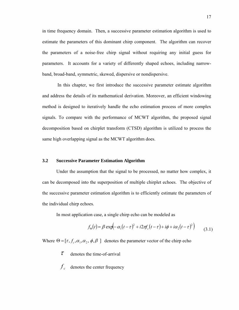
In most application case, a single chirp echo can be modeled as

( ) ( ) ( ) ( )( )22

21 2exp ταφτπταβ −++−+−−=Θ tiitfittf c (3.1)

Where ],,,,,[ 21 βφαατ cf=Θ denotes the parameter vector of the chirp echo

τ denotes the time-of-arrival

cf denotes the center frequency

18

1α denotes the bandwidth factor

2α denotes the chirp-rate

φ denotes the phase

β denotes the amplitude

These parameters can be estimated successively using the chirplet transform (CT).

The successive parameter estimation algorithm is a recursive method that starts with a

time-frequency (TF) representation of the superimposed chirp signal based on the CT.

The CT of ( )tf Θ with respect to a chirplet kernel ( )tΘ

Ψ ˆ is defined as

( ) ( ) dtttfCT ∫

+∞

∞− ΘΘ Ψ=Θ )(ˆ *ˆ

(3.2)

Where ⎥⎦⎤

⎢⎣⎡=Θ ηθγγ

πω ,,,,2

,ˆ21

0

ab denotes the parameter vector of chirplet kernel. The

chirplet kernel ( )tΘ

Ψ ˆ is

( ) ( ) ( ) ⎟⎟

⎠

⎞⎜⎜⎝

⎛−++⎟

⎠⎞

⎜⎝⎛ −

+−−=ΨΘ

220

21ˆ exp btii

abtibtt γθωγη

(3.3)

Where ( )tΘΨ ˆ* denotes the conjugate of ( )tΘ

Ψ ˆ . In order to normalize the energy of the

chirplet kernel, the term 41

12⎟⎠⎞

⎜⎝⎛=πγη . Hence, the CT of a signal chirp echo ( )tfΘ given by

Equation 3.2 can be expressed as

19

( ) ( )

( ) ( )

( ) ( ) ( )

( ) ( ) ( )

⎥⎥⎥⎥

⎦

⎤

+−+

−⎟⎠⎞

⎜⎝⎛ ++−

+

+−+−+−

−

−+

⎢⎢⎢⎢⎢

⎣

⎡

+−+

⎟⎠⎞

⎜⎝⎛ −

−

+−+=Θ

2211

21210

2211

22121

2211

20

2211

41

1

4exp

12ˆ

γαγα

τγγωααω

γαγατγγαα

θφγαγα

ωω

γαγαπγβ

ii

biiia

i

iibii

iii

a

iiCT

c

c

(3.4)

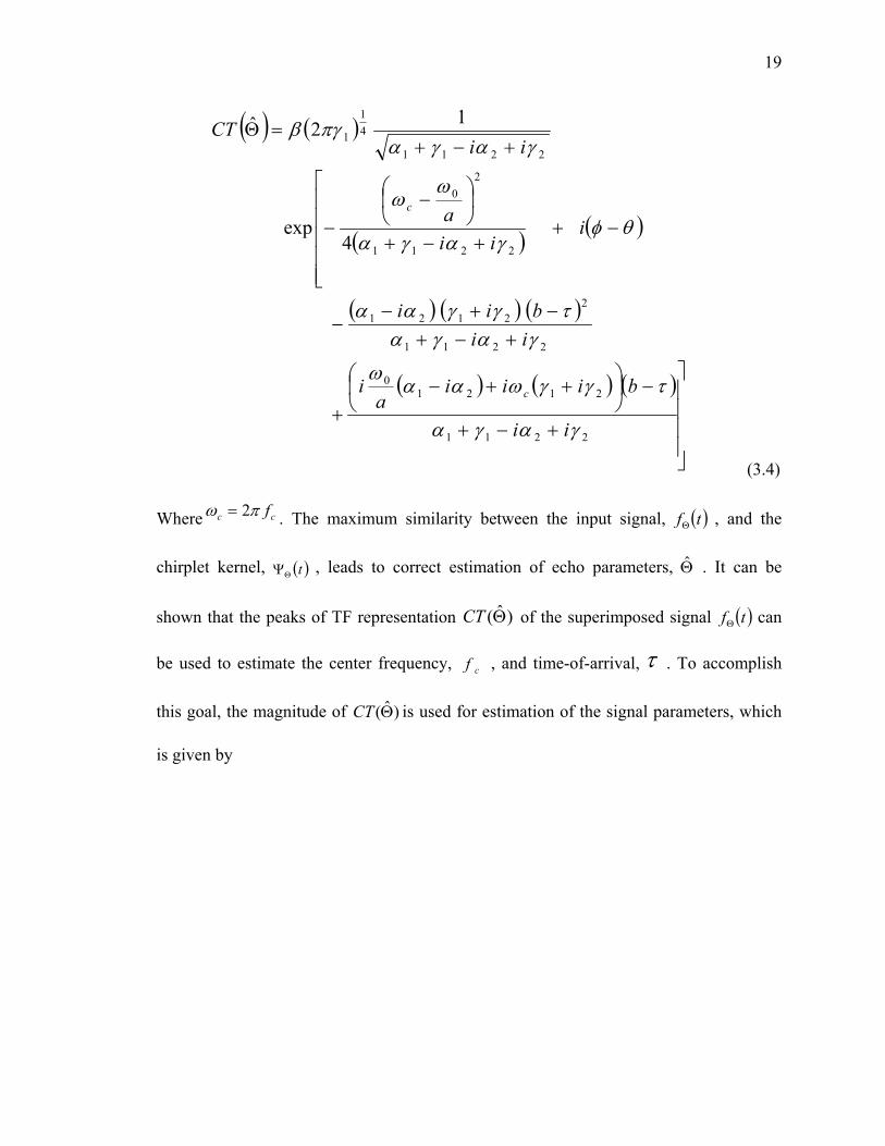
Where cc fπω 2= . The maximum similarity between the input signal, ( )tfΘ , and the

chirplet kernel, ( )tΘΨ , leads to correct estimation of echo parameters, Θ̂ . It can be

shown that the peaks of TF representation )ˆ(ΘCT of the superimposed signal ( )tfΘ can

be used to estimate the center frequency, cf , and time-of-arrival, τ . To accomplish

this goal, the magnitude of )ˆ(ΘCT is used for estimation of the signal parameters, which

is given by

20

( ) ( ) ( ) ( )[ ]

( )

( ) ( )( )

( )( )

( ) ( )( )( )

( ) ( ) ⎥⎥⎦

⎤

−++

−+++−

−++

−+⎟⎠

⎞⎜⎝

⎛ −−

⎢⎢⎢⎢⎢

⎣

⎡

−++

+⎟⎠

⎞⎜⎝

⎛ −−

−++=Θ−

222

211

21

221

211

221

21

222

211

12210

222

211

211

20

412

222

114

11

4exp

2ˆ

γαγαταγαγγαγα

γαγα

τγαγαω

ω

γαγα

γαω

ω

γαγαπγβ

b

ba

a

CT

c

c

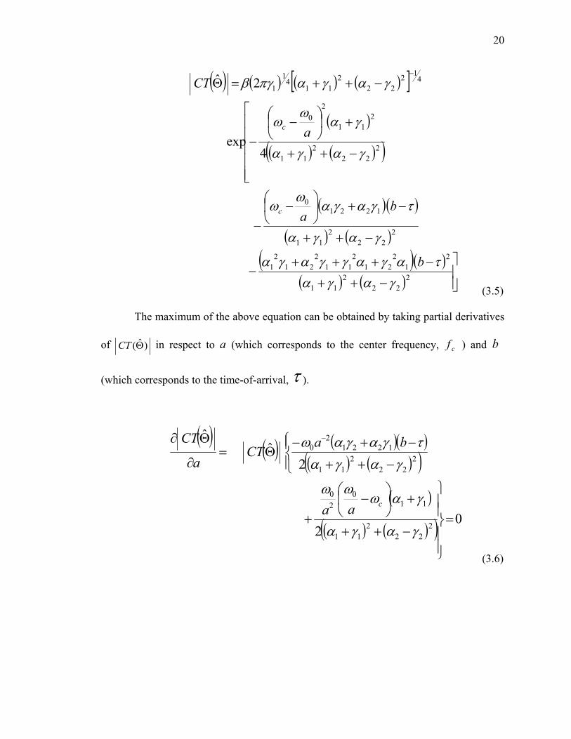
(3.5)

The maximum of the above equation can be obtained by taking partial derivatives

of )ˆ(ΘCT in respect to a (which corresponds to the center frequency, cf ) and b

(which corresponds to the time-of-arrival, τ ).

( ) ( ) ( )( )( ) ( )( )

( )

( ) ( )( ) 02

2ˆ

ˆ

222

211

110

20

222

211

12212

0

=

⎪⎪⎭

⎪⎪⎬

⎫

−++

+⎟⎠

⎞⎜⎝

⎛ −+

⎪⎩

⎪⎨⎧

−++

−+−Θ=

∂

Θ∂ −

γαγα

γαωωω

γαγατγαγαω

caa

baCT

a

CT

(3.6)

21

( ) ( ) ( )( )( ) ( )( )

( )

( ) ( )( ) 04

2ˆ

ˆ

222

211

12210

222

211

221

2111

221

21

=

⎪⎪⎭

⎪⎪⎬

⎫

−++

+⎟⎠

⎞⎜⎝

⎛−

+

⎪⎩

⎪⎨⎧

−++

−+++−Θ=

∂

Θ∂

γαγα

γαγαωω

γαγατγαγαγαγα

ca

bCT

b

CT

(3.7)

The solutions of Equation 3.6 and Equation 3.7 are

τ=b caωω

=0 (3.8)

It is important to point out that under the condition of Equation 3.8, the estimation

of the peak position of )ˆ(ΘCT in TF domain is not a function of the bandwidth factor,

1γ ,chirp-rate, 2γ , and phase, θ of the echo. Furthermore, the peak value of )ˆ(ΘCT is

proportional to the amplitude of the actual echo and leads to the estimation of β .

Based on the above estimations of a and b , the estimation of the chirp-rate, 2γ ,

becomes a one-dimensional estimation problem. This can be achieved by taking the

derivative of )ˆ(ΘCT in respect to 2γ and setting it to 0,

22

( ) ( )( ) ( )( )

( ) ( )

( ) ( )

( ) ( )

( ) ( )( )( ) ( )( )

( ) ( )( )( ) ( ) ( )

( ) ( )( ) ⎥⎥⎦

⎤

−++

−+++−−

−++

−+⎟⎠

⎞⎜⎝

⎛−−

−

−++

+⎟⎠

⎞⎜⎝

⎛−−

−

−++

−+−⎟⎠

⎞⎜⎝

⎛−

−

⎢⎢⎣

⎡

−++

−Θ=

∂

Θ∂

2222

211

21

221

211

221

2122

2222

211

12210

22

2222

211

211

20

22

222

211

212

01

222

211

22

2

2

2

2

2

2ˆ

ˆ

γαγα

ταγαγγαγαγα

γαγα

τγαγαω

ωγα

γαγα

γαω

ωγα

γαγα

ταγτω

ωα

γαγαγα

γ

b

ba

a

bba

CTCT

c

c

c

(3.9)

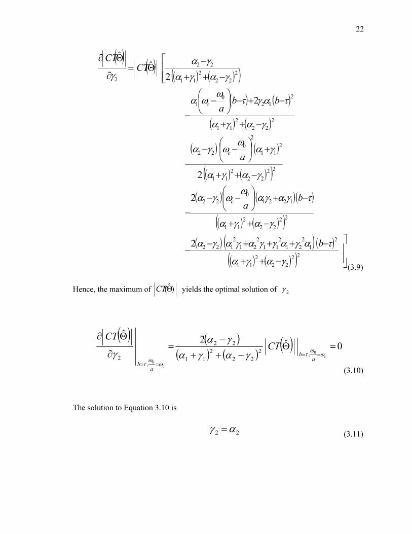
Hence, the maximum of )ˆ(ΘCT yields the optimal solution of 2γ

( ) ( )( ) ( )

( ) 0ˆ2ˆ

0

0

,222

211

22

,2

=Θ−++

−=

∂

Θ∂

==

==c

ca

b

ab

CTCT

ωω

τ

ωω

τγαγα

γαγ

(3.10)

The solution to Equation 3.10 is

22 αγ = (3.11)

23

Similarly, the estimation of the bandwidth factor, 1γ , is carried out by taking the

partial derivative of )ˆ(ΘCT in respect to the bandwidth factor, 1γ , and setting it to 0.

( ) ( ) ( ) ( )( ) ( )( )

( )

( ) ( )( )( ) ( )( )

( ) ( )

( )

( ) ( )( )( ) ( )( )

( ) ( )( )( )( )( )

( ) ( )( ) ⎥⎥⎦

⎤

−++

−++++−

−++

−+⎟⎠⎞

⎜⎝⎛ −+

−

−++

+⎟⎠⎞

⎜⎝⎛ −

−

−++

−++−⎟⎠⎞

⎜⎝⎛ −

−

−++

+⎟⎠⎞

⎜⎝⎛ −

−

⎢⎣

⎡

−++−+−

Θ=∂

Θ∂

2222

211

21

221

211

221

2111

2222

211

12210

11

2222

211

311

20

222

211

222

21

02

2222

211

11

20

222

2111

222

21

21

1

2

2

2

2

4ˆ

ˆ

γαγα

ταγαγγαγαγα

γαγα

τγαγαωωγα

γαγα

γαωω

γαγα

ταατωωα

γαγα

γαωω

γαγαγγαγα

γ

b

ba

a

bba

a

CTCT

c

c

c

c

(3.12)

Hence,

( )( )

( ) 0ˆ4

ˆ

22

0

22

0

,

,2

111

21

21

,

,1

=Θ⎟⎟⎠

⎞⎜⎜⎝

⎛

+−

=∂

Θ∂

=

=

=

=

=

=

αγω

ωτ

αγω

ωτ γαγ

γαγ c

ca

b

a

bCT

CT

(3.13)

The solution to Equation 3.13 yields

24

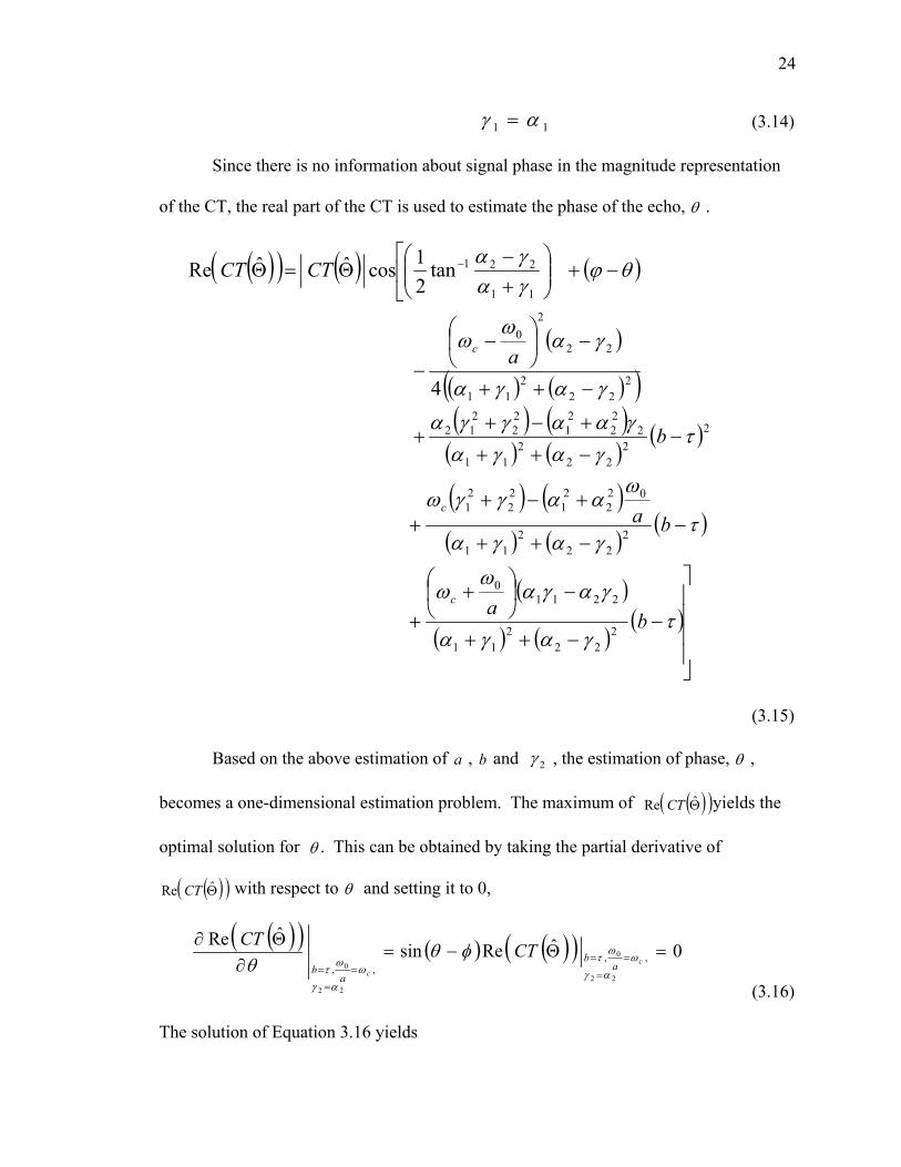
11 αγ = (3.14)

Since there is no information about signal phase in the magnitude representation

of the CT, the real part of the CT is used to estimate the phase of the echo, θ .

( )( ) ( ) ( )

( )

( ) ( )( )( ) ( )( ) ( )

( )

( ) ( )( ) ( )

( )

( )

( ) ( )( )

⎥⎥⎥⎥

⎦

⎤

−−++

−⎟⎠

⎞⎜⎝

⎛ ++

−−++

+−++

−−++

+−++

−++

−⎟⎠

⎞⎜⎝

⎛ −−

−+⎢⎣

⎡⎟⎟⎠

⎞⎜⎜⎝

⎛+−

Θ=Θ −

τγαγα

γαγαω

ω

τγαγα

ωααγγω

τγαγα

γααγγα

γαγα

γαω

ω

θϕγαγα

ba

ba

b

a

CTCT

c

c

c

222

211

22110

222

211

022

21

22

21

22

222

11

222

21

22

212

222

211

22

20

11

221

4

tan21cosˆˆRe

(3.15)

Based on the above estimation of a , b and 2γ , the estimation of phase, θ ,

becomes a one-dimensional estimation problem. The maximum of ( )( )Θ̂Re CT yields the

optimal solution for θ . This can be obtained by taking the partial derivative of

( )( )Θ̂Re CT with respect to θ and setting it to 0,

( )( ) ( ) ( )( ) 0ˆResinˆRe

22

0

22

0,,

,,=Θ−=

∂Θ∂

=

==

=

== αγω

ωτ

αγω

ωτ

φθθ c

ca

b

ab

CTCT

(3.16)

The solution of Equation 3.16 yields

25

πφθ k2±= , ,...3,2,1=k (3.17)

In summary, the mathematical steps present above show that the chirplet

transform leads to an exact estimation of the time-of-arrival, center frequency, phase,

bandwidth factor, and chirp-rate of the chirp echo signal. The parameter estimation based

on these equations can be implemented successively using signal correlation (see

Equation 3.2). A grid search is performed of these parameters are refined with a fast

Gauss-Newton algorithm [Dem00, Dem01a, Dem01b]. The refinement improves the

parameter estimation beyond the resolution of the search grid. The successive parameter

estimation based on CTSD method can recover the exact value of the parameters of a

noise-free Gaussian chirp echo. It does not require any initial guess for the parameters

before estimation. Furthermore, it can also estimate the parameters of a noise corrupted

echo with high accuracy.

3.3 Windowing Algorithm

We utilize the successive parameter estimation technique to decompose a

complex signal into a small number of Gaussian chirplets. The complex signal is

presented by the linear addition of a number of chirplets:

( )∑

−

=Θ=

1

0)(

N

jtfts

j

(3.18)

where ( )tfjΘ is the chirplet model and jΘ is the parameter vector of ( )tf

jΘ , (refer to

Equation 3.1).

26

The goal of signal decomposition is to express the signal, )(ts , as a linear

combination of chirp components. The decomposition is performed as follows. First,

based on the CT of the signal (i.e.,TF representation), the most dominant chirp echo is

windowed and estimated using the successive parameter estimation algorithm presented

in Section 3.2. Then, the estimated echo is subtracted from the original signal. Next, the

second echo is estimated from the remaining signal. This process is repeated until the

reconstruction error, Er, is below an acceptable value Emin. The value of Emin is

determined based on the requirements of the reconstruction quality of the signal. This

iterative decomposition method ensures energy preservation by coherently distributing

the signal energy into composing function. Energy preservation allows us to add the TF

distribution of composing function ( )tfjΘ to estimate the TF distribution of the

signal )( ts . Meanwhile, the sparseness of decomposition is ensured by searching for

the most dominant chirp echo per iteration. A block diagram summarizing the chirplet

signal decomposition algorithm is shown in Figure 3.1.

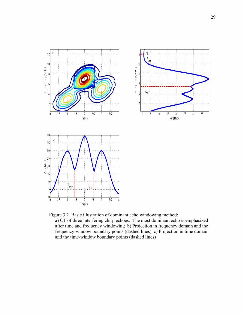
The procedure used to design the window is based on the determination of the

peaks and valleys of the CT of the signal. Figure 3.2 illustrates the windowing method

with simulated data containing 3 interfering echoes. First, the maximum peak of the CT

of the signal (Figure. 3.2a) is identified. Next, the CT of the signal is projected onto the

time domain (Figure. 3.2c) and frequency domain (Figure. 3.2b). The windowing

algorithm uses these projections to isolate the dominant echo by tracing the nearest

valleys around the peak. The closest two valleys confining the time-projection peak are

defined as the boundaries of the time-window (i.e., Tbegin and Tend in Figure. 3.2c).

Similarly, the closest two valleys confining the frequency projection peak are defined as

27

the boundaries of the frequency-window (i.e., Fbegin and Fend in Figure 3.2b). The time-

of-arrival τ and center frequency cf parameters are in fact the peak locations of the

projections (see Equation 3.2). The dominant signal along with the time window and

frequency window is used to estimate the remaining chirplet parameters (i.e.,

amplitude β , bandwidth 1γ , chirp rate 2γ , and phaseθ ) using signal correlation (see

Equation 3.2).

When there are heavily overlapping echoes and high noise levels, the performance

of the automatic windowing method may be compromised as the peak separation process

becomes more difficult. The distance between peaks becomes shorter and artificial

valley points may be created due to the noise. In these cases, a time window and

frequency window with predetermined size can be used to separate out the time and

frequency projection peaks. The windows are centered at the peaks. The sizes of the

windows can be determined by inspecting the CT of the measured signal for given noise

levels. A good window size selection strategy is to keep as much of the signal energy as

possible while suppressing the contribution of noise energy in the window. For the

simulated and experimental signals presented in this study, the automatic windowing

method performed adequately in extracting the individual echoes. However, one can

apply the predetermined windowing method for signals with very poor SNRs (2 dB and

below).

28

E stim ate α 2 ,α 1 and φ

E r < E m in

Y es

N o Subtract the estim ated

echo from the signal

S tore the estim ated param eters

G enerate ( )Θ̂C T and

localize dom inant echo

by w indow ing m ethod

M ultip le E choes

C alculate reconstruction error E r

E stim ate β , fc and τ

Figure 3.1 The Flowchart of the CTSD Algorithm.

29

Figure 3.2 Basic illustration of dominant echo windowing method: a) CT of three interfering chirp echoes. The most dominant echo is emphasized after time and frequency windowing b) Projection in frequency domain and the frequency-window boundary points (dashed lines) c) Projection in time domain and the time-window boundary points (dashed lines)

30

3.4 Comparison with Gabor Decomposition Algorithm

The CTSD algorithm is very effective in representing dispersive ultrasonic

echoes. An alternative decomposition algorithm [Car05a] uses a Gabor kernel to analyze

ultrasonic echoes. However, if the ultrasonic signal has a dispersive or frequency shift

property, Gabor decomposition requires many components. The chirplet model is

expected to have better decomposition efficiency with extra parameter diversity. To

demonstrate chirplet decomposition efficiency, a noisy chirp signal containing highly

overlapping echoes is simulated, and then the algorithm presented in [Car05a] and the

CTSD algorithm are both applied to reconstruct the signal. Figure 3.3 shows the noisy

chirp signal and the two reconstruction results from these two different decomposition

strategies, under the same output SNR criteria. More specifically, the parameters of the

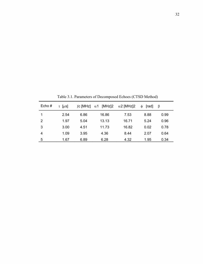
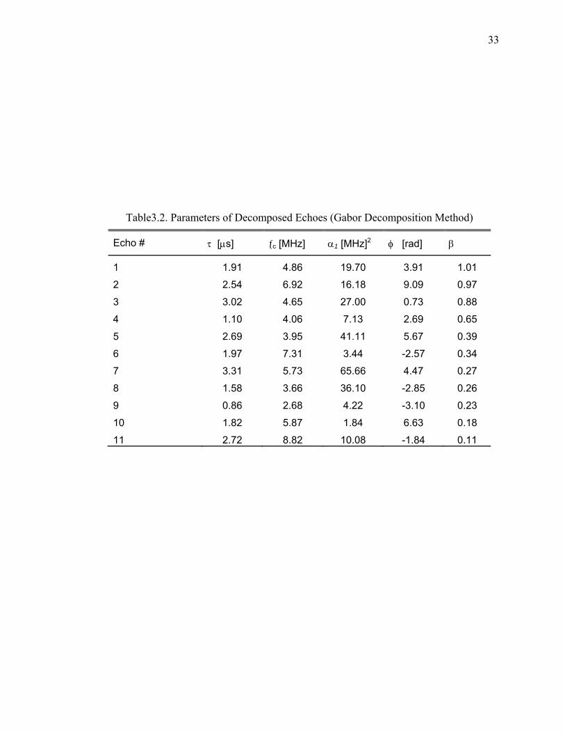
decomposed echoes are listed in Table 3.1 and Table 3.2. Furthermore, Figure 3.4 shows

the time frequency difference of the reconstructed signal using CTSD method (see Figure

3.4c and Figure 3.4d) and using Gabor method (see Figure 3.4e and Figure 3.4f). It can

be seen that, under the same quality of reconstructed signal (i.e., the same output SNR

criteria), the chirplet decomposition algorithm requires significantly a less number of

components than Gabor decomposition [Lu06a].

The compact representation achieved by the chirplet decomposition is more

powerful in revealing the physical properties of chirp-type signals (e.g., the Doppler shift

in a radar system, the dispersive echoes in an ultrasonic nondestructive testing system).

31

3.5 Summary

In this chapter, we introduce a successive and efficient chirplet decomposition

algorithm that employs an adaptive chirplet kernel as the general model for the parameter

estimation of the superimposed chirp signal. This algorithm adaptively tracks and locates

the individual echoes for efficient and precise estimation of all echo parameters. Analysis

results showed that the performance of chirplet signal decomposition overwhelmed that

of the Gabor decomposition algorithm with less number of components to reconstruct the

same high overlapping signal. Hence, the chirplet signal decomposition and parameter

estimation algorithm allows for high fidelity signal reconstruction.

32

Table 3.1. Parameters of Decomposed Echoes (CTSD Method)

Echo # τ [μs] ƒc [MHz] α1 [MHz]2 α2 [MHz]2 φ [rad] β

1 2.54 6.86 16.86 7.53 8.88 0.99

2 1.97 5.04 13.13 16.71 5.24 0.96

3 3.00 4.51 11.73 16.82 0.02 0.78

4 1.09 3.95 4.36 8.44 2.07 0.64

5 1.67 6.89 6.28 4.32 1.95 0.34

33

Table3.2. Parameters of Decomposed Echoes (Gabor Decomposition Method)

Echo # τ [μs] ƒc [MHz] α1 [MHz]2 φ [rad] β

1 1.91 4.86 19.70 3.91 1.01

2 2.54 6.92 16.18 9.09 0.97

3 3.02 4.65 27.00 0.73 0.88

4 1.10 4.06 7.13 2.69 0.65

5 2.69 3.95 41.11 5.67 0.39

6 1.97 7.31 3.44 -2.57 0.34

7 3.31 5.73 65.66 4.47 0.27

8 1.58 3.66 36.10 -2.85 0.26

9 0.86 2.68 4.22 -3.10 0.23

10 1.82 5.87 1.84 6.63 0.18

11 2.72 8.82 10.08 -1.84 0.11

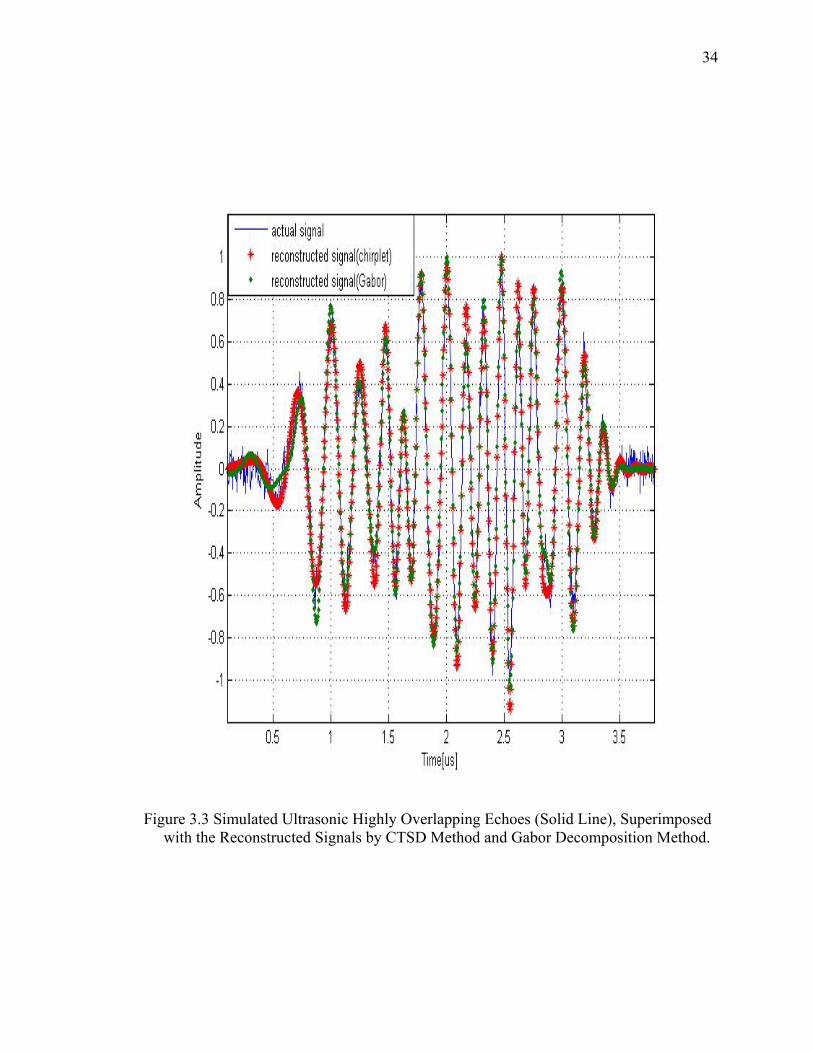
34

Figure 3.3 Simulated Ultrasonic Highly Overlapping Echoes (Solid Line), Superimposed with the Reconstructed Signals by CTSD Method and Gabor Decomposition Method.

35

Figure 3.4. Comparisons of CTSD Method and Gabor Decomposition Method. a) Simulated Highly Overlapping Echoes. b) WVD of the Original Simulated Signal. c) Reconstructed Signal by CTSD Method. d) WVD of the Reconstructed Signal (Using CTSD). e) Reconstructed Signal by Gabor Method. f) WVD of the Reconstructed Signal (Using Gabor).

36

CHAPTER 4

SIGNAL DECOMPOSITION BASED ON MATCHING PURSUIT

4.1 Introduction

The matching pursuit (MP) algorithm has been initially introduced by Mallat and

Zhang [Mal89, Mal93]. It aims to provide a signal analysis framework for non-stationary

signal under energy conservation signal decomposition condition. Hence, a high

resolution TF representation can be achieved by decomposing ultrasonic backscattering

signal into a limited number of elementary functions with known TF distribution such as

WVD.

The real challenge of matching pursuit algorithm is that different matching

criteria can get different decomposition results [Adl96, Che98, and Cot98]. The original

matching pursuit algorithm uses correlation criteria (the inner product between signal

residue and a pre-defined dictionary function) to determine the best matching function.

This matching criterion obtains decompositions adaptive to global signal characteristics,

but is not best adapted to its local structures.

Recently, an enhanced version of MP algorithm, called high resolution matching

pursuit (HRMP) algorithm, is proposed by Grilbonval et. al [Gri96]. The HRMP uses a

different correlation function, which allows the pursuit to emphasize local fit over global

fit at each step. The new correlation function avoids creating energy at time location

where there are none. Compared with MP algorithm, HRMP algorithm performs higher

time resolution decomposition but the frequency resolution is decreased [Gri96]. This

limits the use of HRMP algorithm in the case for ultrasonic signal where local signal

structure change in frequency.

37

In this chapter, we first introduce matching pursuing signal decomposition

algorithm based on Maximum Likelihood Estimation (MPSD-MLE). The principle of

MPSD-MLE algorithm is discussed. Moreover, another implementation scheme, which is

the matching pursuit signal decomposition based on Maximum a Posteriori (MPSD-

MAP), is presented. Furthermore, the performance of these two algorithms is

demonstrated by applying both algorithms to simulated overlapping signal.

4.2 MPSD-MLE Algorithm

In the implementation of the original MP algorithm, the best match criterion is

based on the projection coefficient obtained by projecting the signal residue of current

stage onto a dictionary function. The signal residue of next stage is the remaining signal

after the best matching function has been subtracted from the signal residue of current

stage. When the energy summation of signal residue at all stages is a fraction of the

energy of the original signal, the decomposition is said to be completed. The final

decomposition is a linear expansion of all chosen matching functions.

In our MP algorithm, by incorporating the statistical strategies such as Maximum

Likelihood Estimation (MLE) and Maximum a Posteriori (MAP) method, we adaptively

optimize the parameters of the chirplet function to achieve high resolution

decompositions. This approach avoids the exhaustive search of a larger number of

dictionary functions and leads to a more efficient implementation.

At any stage of the MP algorithm, the signal residue is represented by a chirplet

function and a remaining signal (i.e., next residue),

38

sRtgsR nn 1);( ++Θ= (4.1)

Here, sR n is the current residue of signal )(ts , sR n 1+ is the next signal residue and

);( Θtg is a chirplet echo defined by the model,

])()(2cos[);( 22

2)( 21 φτατπβ τα +−+−=Θ −− ttfetg c

t

(4.2)

Where ],,,,,[ 21 τφβαα cf=Θ denotes the parameter vector of );( Θtg .

If we assume sR n 1+ has white Gaussian noise characteristics, the maximum likelihood

estimation of the parameter vector Θ can be obtained by minimizing:

2);(minargˆ Θ−=Θ Θ tgsR n

MLE (4.3)

Therefore, the parameter vector of the best matching function at stage n is chosen

by minimizing the least-square error. By assuming the remaining signal residue sR n 1+

is white Gaussian, Maximum Likelihood Estimation is simplified to Least Square

estimation [Kay93, Dem01a]. Hence, the optimization problem in Equation 4.3 replaces

the search for the best matching function. The MLE parameter vector, MLEΘ̂ , maximizes

the inner product between signal residue and normalized chirplet function, );(, ΘtgsR n .

In summary, for the signal )(ts , the MPSD-MLE algorithm can be outlined in

the following computation steps:

1. Set iteration index 0=n and first signal residue )(0 tssR = .

2. Find the best parameter vector of the chirplet function such that

2

);(minargˆ Θ−=Θ Θ tgsRnn (4.4)

39

3. Computer the next residue )ˆ;(1n

nn tgsRsR Θ−=+.

4. Check convergence: If Thresholdts

sR n

≤+

2

21

)(, STOP;

OTHERWISE, set 1+→ nn , and go to Step 2.

Step 1 of the algorithm initializes current signal residue as the original signal.

Step 2 finds the best matching function for the current signal residue by optimizing the

parameters of the chirplet function. Step 3 computes the next signal residue by

subtracting the best matching chirplet function. Step 4 checks for convergence: if the

residue energy is some fraction of the original signal energy, the algorithm stops,

otherwise a new chirplet function is matched to current signal residue. The flow chart of

MPSD algorithm is shown in Figure 4.1.

In the decomposition algorithm, Step 2 is essentially the most important step. An

optimal solution is critical in achieving the best decomposition. Since the model );( Θtg

is a nonlinear function ofΘ , there is no closed form solution available for Equation 4.4.

An iterative estimator can be obtained by successive linearizing the objective function.

i.e., by taking Taylor series expansion of );( Θtg at ( )nΘ

))(();();( )()()( nnn Htgtg Θ−ΘΘ+Θ≈Θ (4.5)

Where )(

)()( )(

n

gH n

Θ=ΘΘ∂Θ∂

=Θ

Then Equation 4.5 can be expressed as

WHX n +ΘΘ= )(~ )( (4.6)

Where ( ) )()()( )(;~ nnnn HtgsRX ΘΘ+Θ−= , and sRW n 1+=

Lemma 1: Optimality of the MLE for the linear model [Kay98]

40

For linear model WHX +Θ= , where ),0(~ WCNW .Then the minimum variance

unbiased MVU estimator is XHHH TT 1][ˆ −=Θ . Therefore, assuming that sR n 1+ has

white Gaussian noise (WGN) characteristics in Equation 4.6, the MLE estimation of the

parameter vector Θ can be obtained by

)];()[()]()([ˆ )(1)()()( nnnTnnTnMLE tgsRHHH Θ−ΘΘΘ+Θ=Θ −

(4.7)

A fast Gauss-Newton algorithm is used to approach the MLE estimator MLEΘ̂ in

iterative manner. Consider the signal sR n and the chirp function );( Θtg [see Equation

4.2]

it can be outlined as the following steps.

1. Make an initial guess for the parameter vector )0(Θ and set iteration number

0=k .

2. Compute the gradients ( ) )( kH Θ of the chirplet function );( )( ktg Θ .

3. Update the parameter vector:

( ) ( )[ ] ( ) ( ) )];()[()()( 1)()1( knkTkkTkkMLE tgsRHHH Θ−ΘΘΘ+Θ=Θ

−+ (4.8)

4. Check convergence: If Thresholdkk ≤Θ−Θ + )()1( , then STOP;

OTHERWISE, set 1+→ kk , and go to Step 2.

The MPSD-MLE method described above yields a greedy approximation of the

signal. As long as a function matches the signal residue, it is included in the

decomposition. We demonstrate the performance of MPSD-MLE with a simulation

41

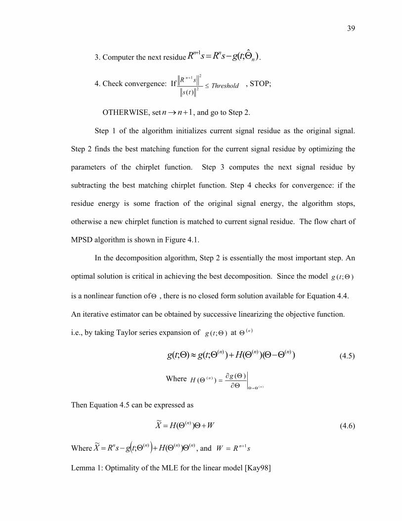
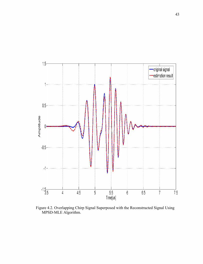
example. This example simulates two overlapping ultrasonic echoes sampled at 100 MHz

sampling frequency. The parameter vectors used to generate these functions are

[ ]0.10.0][0.4][0.80.40.5 221 radMHzMHzMHzsμ=Θ

[ ]0.10.1][0.3][0.60.65.5 222 radMHzMHzMHzsμ=Θ

These two echoes are very close in terms of center frequency and bandwidths.

Figure 4.2 shows the overlapping signal superimposed with the reconstructed result.

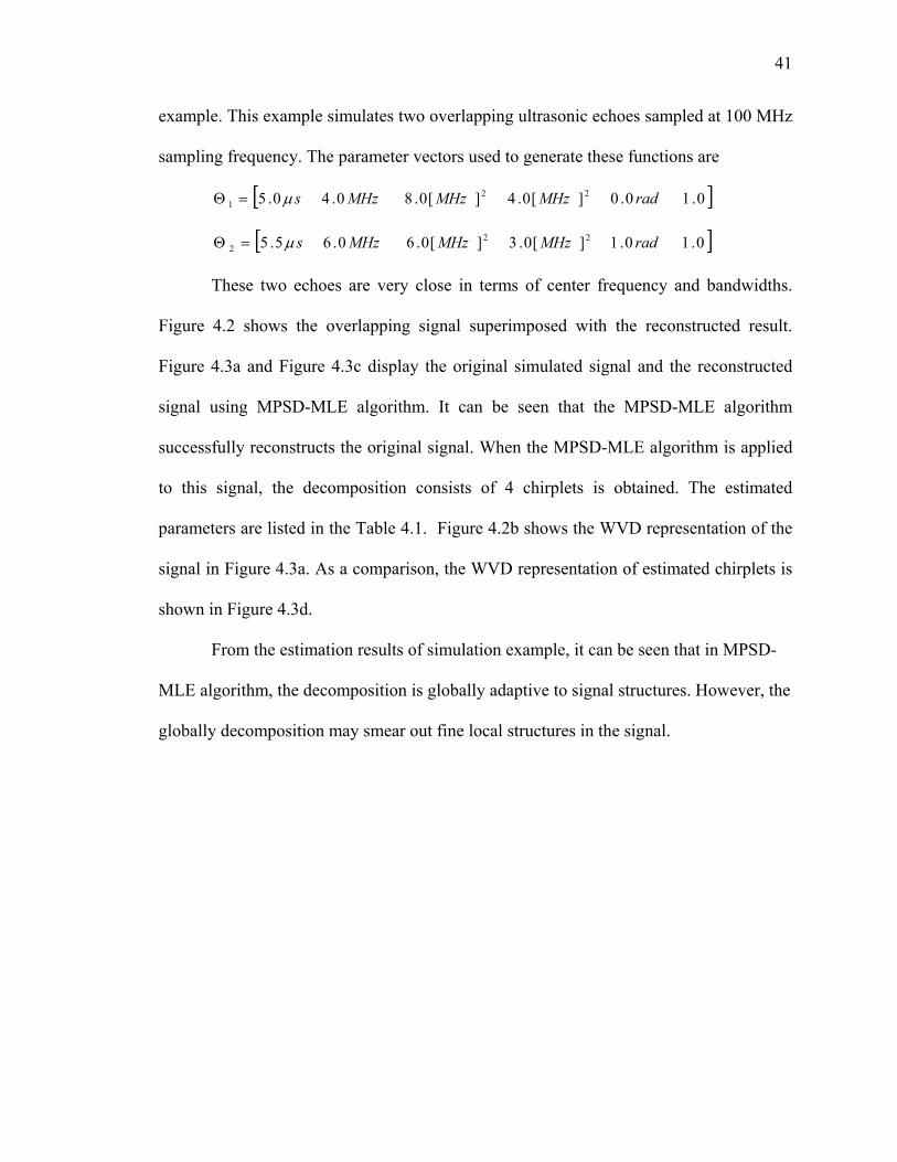
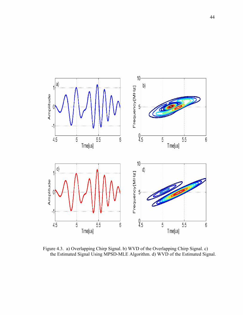
Figure 4.3a and Figure 4.3c display the original simulated signal and the reconstructed

signal using MPSD-MLE algorithm. It can be seen that the MPSD-MLE algorithm

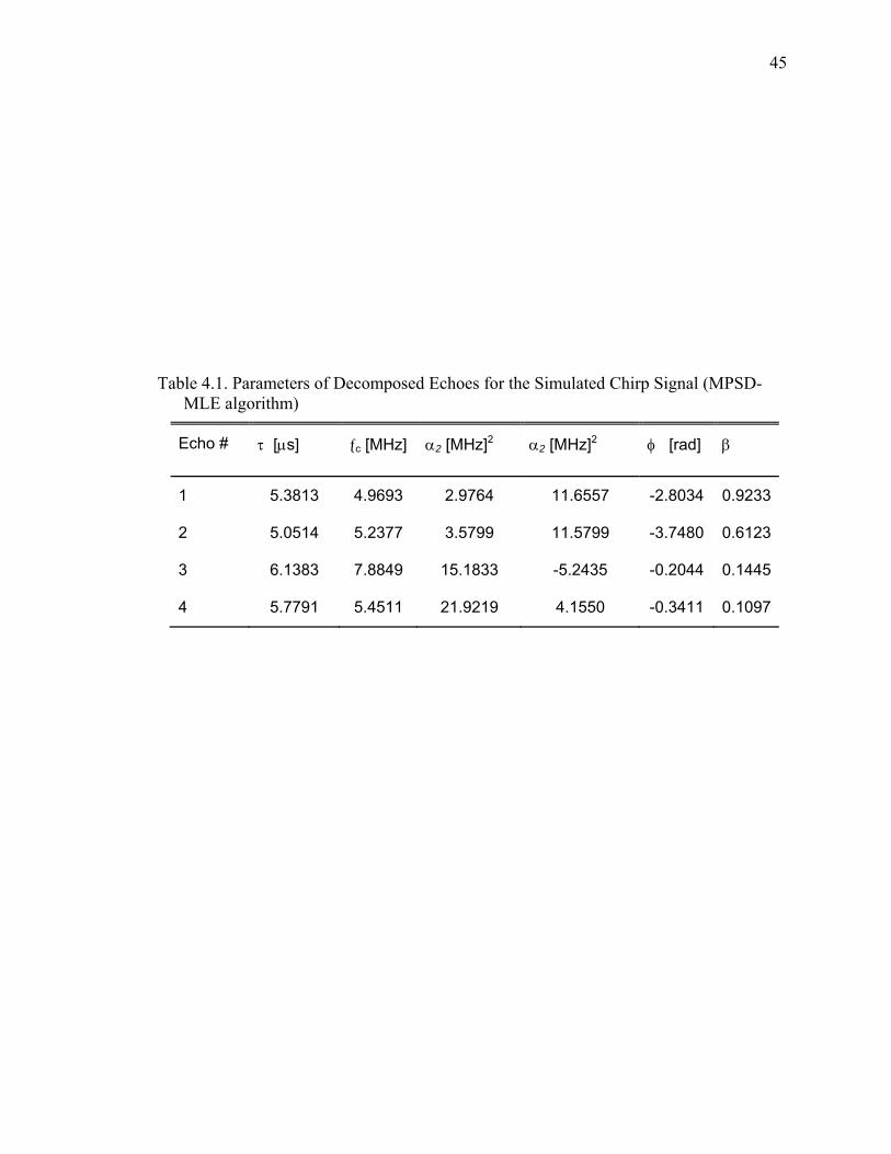
successfully reconstructs the original signal. When the MPSD-MLE algorithm is applied

to this signal, the decomposition consists of 4 chirplets is obtained. The estimated

parameters are listed in the Table 4.1. Figure 4.2b shows the WVD representation of the

signal in Figure 4.3a. As a comparison, the WVD representation of estimated chirplets is

shown in Figure 4.3d.

From the estimation results of simulation example, it can be seen that in MPSD-

MLE algorithm, the decomposition is globally adaptive to signal structures. However, the

globally decomposition may smear out fine local structures in the signal.

42

Figure 4.1. The Flowchart of MPSD Algorithm.

43

Figure 4.2. Overlapping Chirp Signal Superposed with the Reconstructed Signal Using MPSD-MLE Algorithm.

44

Figure 4.3. a) Overlapping Chirp Signal. b) WVD of the Overlapping Chirp Signal. c) the Estimated Signal Using MPSD-MLE Algorithm. d) WVD of the Estimated Signal.

45

Table 4.1. Parameters of Decomposed Echoes for the Simulated Chirp Signal (MPSD- MLE algorithm)


1 5.3813 4.9693 2.9764 11.6557 -2.8034 0.9233

2 5.0514 5.2377 3.5799 11.5799 -3.7480 0.6123

3 6.1383 7.8849 15.1833 -5.2435 -0.2044 0.1445

4 5.7791 5.4511 21.9219 4.1550 -0.3411 0.1097

46

4.3 MPSD-MAP Algorithm

One can improve the MPSD algorithm by concentrating on the local signal

structures and using better matching criteria. We propose a MPSD algorithm based on

the MAP estimation principle to achieve high-resolution decompositions. This algorithm

is an extension of the MPSD-MLE algorithm. Essentially, the MAP strategy replaces the

MLE strategy in Step 2: when choosing the chirplet function to match signal residues,

one can place constraints on the parameters of chirplet functions to achieve locally

adaptive functions. By enforcing a priori information on the parameters of chirplet

functions, MAP estimation provides a convenient and highly effective way to match local

signal characteristics. This estimation approach also uses the least square criterion but

only includes chirplet functions whose parameters are allowed to vary around a priori

values in the decomposition.

The MPSD-MAP algorithm can be formulated by changing Step 2 of the MPSD-

MLE algorithm as:

2);(minargˆ Θ−=Θ Θ tgsR n

n , where Θ=Θ μ)(E and Θ=ΘΘ CE T )( (4.9)

Based on the above optimization criterion, the MAP estimator can be derived as

following.

Lemma 2: Posterior probability density function (PDF) for the Bayesian General

Linear Model [Kay98 ]

For Bayesian general linear model WHX +Θ= , where ),0(~ WCNW and

),(~ ΘΘΘ CN μ .Then the posterior PDF )|( Xp Θ is Gaussian with mean

)()(]|[ 1Θ

−ΘΘΘ −++=Θ μμ HXCHHCHCXE W

TT and covariance

47

Θ−

ΘΘΘΘ +−= HCCHHCHCCC WTT

X1

| )( . Therefore, in Equation 4.6, assuming that

),0(~1W

n CNsR + and ),(~ ΘΘΘ CN μ

The MAP estimation of the parameter vector Θ can be obtained by

)])(();()[()]()([ˆ )()()()(1)()(1Θ

−−ΘΘ −ΘΘ+Θ−ΘΘΘ++=Θ CHtgsRHHHCC nnnnnTnnT

WMAP μ

(4.10)

It can be verified that if there is no prior knowledge of Θ (i.e.,

0=Θμ and ∞=ΘC ), the MAP estimator (see Equation 4.10) is same as the MLE

estimator (see Equation 4.7). Similarly, a fast Gauss-Newton algorithm is used to

approach the MAP estimator MAPΘ̂ in iterative manner. In the Step 3 of fast Gauss-

Newton algorithm, Equation 4.8 is substituted by Equation 4.11.

)])(();()[()]()([ )()()()(1)()(11Θ

−−ΘΘ

+ −ΘΘ+Θ−ΘΘΘ++=Θ CHtgsRHHHCC kkknkTkkTW

kMAP μ

(4.11)

To demonstrate the difference of MPSD-MLE and MPSD-MAP, we apply

MPSD-MAP algorithm to the same overlapping simulated chirp signal in the

demonstrated example of MPSD-MLE discussion. For MPSD-MAP decomposition, the

following prior statistics are used for the parameter vector

[ ]0.10.0][15][250.50.1][ 22 radMHzMHzMHzsE μ=Θ

⎥⎥⎥⎥⎥⎥⎥⎥

⎦

⎤

⎢⎢⎢⎢⎢⎢⎢⎢

⎣

⎡

=Θ

0.10000000.1000000][15000000][2500000020000000.1

2

2

radMHz

MHzMHz

s

C

μ

(4.12)

48

These prior statistics favor chirplet functions with center frequencies around 5

MHz, bandwidth factor around 25 [MHz] 2, chirp rate around 15 [MHz] 2. The variations

in these values are determined by the variances, i.e., the diagonal elements in the

covariance matrix ΘC .

As a comparison of MPSD-MLE algorithm, the same ultrasonic signal is used to

demonstrate the MPSD-MAP algorithm. Figure 4.4 shows the overlapping signal

superimposed with the reconstructed result. Figure 4.5a and Figure 4.5c display the

original simulated signal and the reconstructed signal using MPSD-MAP algorithm. It

can be seen that the MPSD-MAP algorithm successfully reconstructs the original signal.

When the MPSD-MAP algorithm is applied to this signal, the decomposition consists of

3 chirplets is obtained. The estimated parameters are listed in the Table 4.2. Figure 4.5b

shows the WVD representation of the signal in Figure 4.5a. As a comparison, the WVD

representation of estimated chirplets is shown in Figure 4.5d.

From the above results, it can be seen that , unlike the MPSD-MLE

decomposition[see Figure 4.3 and Table 4.1], the MPSD-MAP composition clearly fit

two distinct signal components with slightly different frequency content and produce a

physically meaningful result[see Figure 4.5 and Table 4.2 ].

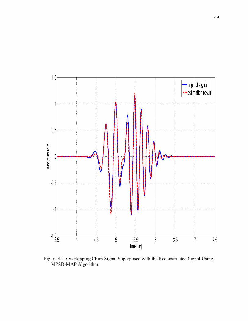
49

Figure 4.4. Overlapping Chirp Signal Superposed with the Reconstructed Signal Using MPSD-MAP Algorithm.

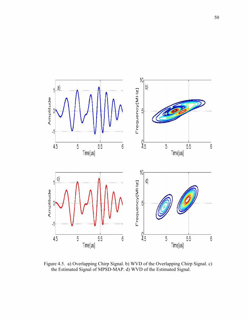
50

Figure 4.5. a) Overlapping Chirp Signal. b) WVD of the Overlapping Chirp Signal. c) the Estimated Signal of MPSD-MAP. d) WVD of the Estimated Signal.

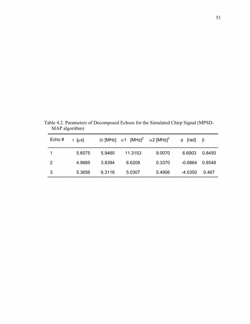
51

Table 4.2. Parameters of Decomposed Echoes for the Simulated Chirp Signal (MPSD- MAP algorithm)


1 5.6575 5.9460 11.3153 9.0070 6.6903 0.8450

2 4.9685 3.8394 6.6208 0.3370 -0.6864 0.8548

3 5.3656 6.3116 5.0307 5.4906 -4.0350 0.467

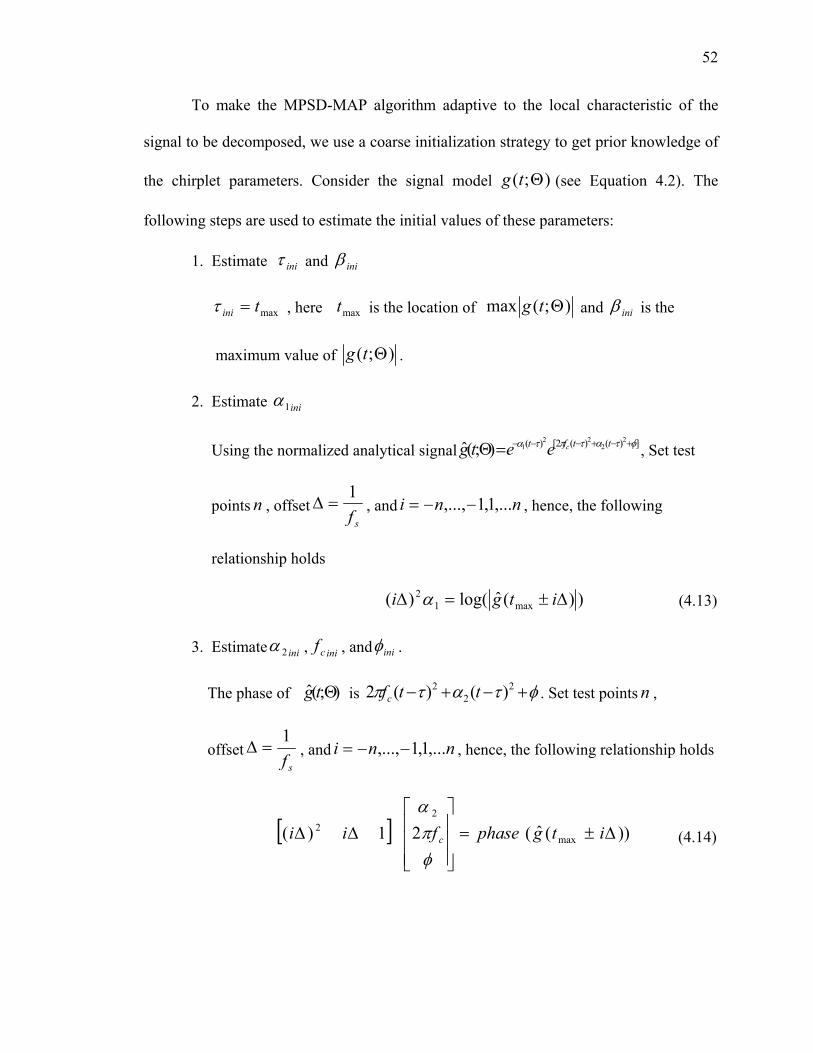
52

To make the MPSD-MAP algorithm adaptive to the local characteristic of the

signal to be decomposed, we use a coarse initialization strategy to get prior knowledge of

the chirplet parameters. Consider the signal model );( Θtg (see Equation 4.2). The

following steps are used to estimate the initial values of these parameters:

1. Estimate iniτ and iniβ

maxtini =τ , here maxt is the location of );(max Θtg and iniβ is the

maximum value of );( Θtg .

2. Estimate ini1α

Using the normalized analytical signal ])()(2[)( 22

221);(ˆ φτατπτα +−+−−−=Θ ttft ceetg , Set test

points n , offsetsf

1=Δ , and nni ,...1,1,...,−−= , hence, the following

relationship holds

))(ˆlog()( max12 Δ±=Δ itgi α (4.13)

3. Estimate ini2α , inicf , and iniφ .

The phase of );(ˆ Θtg is φτατπ +−+− 22

2 )()(2 ttfc . Set test points n ,

offsetsf

1=Δ , and nni ,...1,1,...,−−= , hence, the following relationship holds

[ ] ))(ˆ(21)( max

22 Δ±=

⎥⎥⎥

⎦

⎤

⎢⎢⎢

⎣

⎡ΔΔ itgphasefii c

φπα

(4.14)

53

In Equation 4.13 and Equation 4.14, the initial parameters ini1α , ini2α , inicf ,

and iniφ can be estimated through the n2 test equations, using the least square solution. In

a matrix form, the least square solution of equation BAX = is BAAAX '1' )( −= . It

is also noticed that the initial guess in severe noise levels affects the iteration efficiency

of MPSD algorithm.

4.4 Summary

In this chapter, the matching pursuit signal decomposition algorithm was

presented. By incorporating the MLE and MAP estimation strategies into the original

matching pursuit framework, the experimental and analytical results have shown that

both algorithms can be successfully used to decompose the signal into a linear

combination of chirplets and estimate the parameters of each chirplet. The different

decomposition results verified the difference of the algorithms in the nature of

implementation.

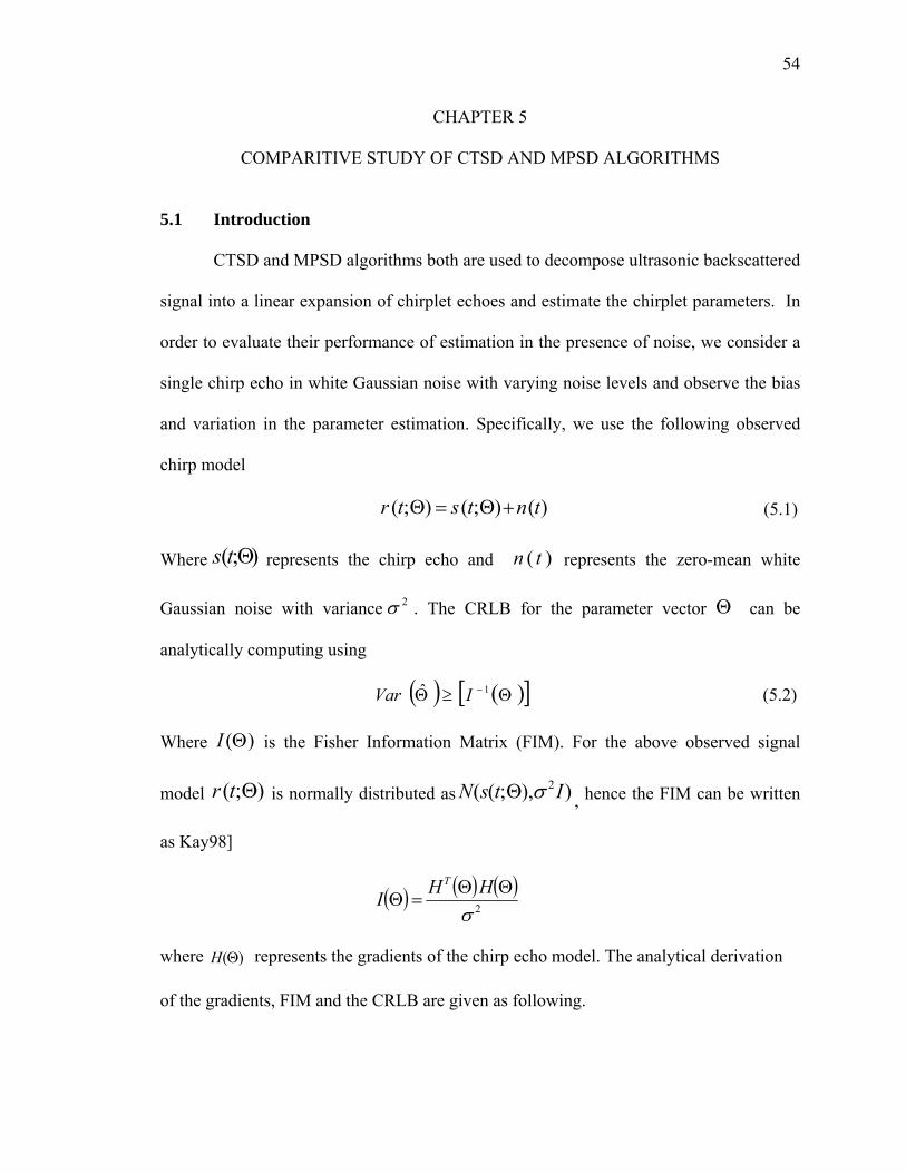
54

CHAPTER 5

COMPARITIVE STUDY OF CTSD AND MPSD ALGORITHMS

5.1 Introduction

CTSD and MPSD algorithms both are used to decompose ultrasonic backscattered

signal into a linear expansion of chirplet echoes and estimate the chirplet parameters. In

order to evaluate their performance of estimation in the presence of noise, we consider a

single chirp echo in white Gaussian noise with varying noise levels and observe the bias

and variation in the parameter estimation. Specifically, we use the following observed

chirp model

)();();( tntstr +Θ=Θ (5.1)

Where );( Θts represents the chirp echo and )( tn represents the zero-mean white

Gaussian noise with variance 2σ . The CRLB for the parameter vector Θ can be

analytically computing using

( ) ( )[ ]Θ≥Θ − 1ˆ IVar (5.2)

Where )(ΘI is the Fisher Information Matrix (FIM). For the above observed signal

model );( Θtr is normally distributed as )),;(( 2ItsN σΘ , hence the FIM can be written

as Kay98]

( ) ( ) ( )2σ

ΘΘ=Θ

HHIT

where )(ΘH represents the gradients of the chirp echo model. The analytical derivation

of the gradients, FIM and the CRLB are given as following.

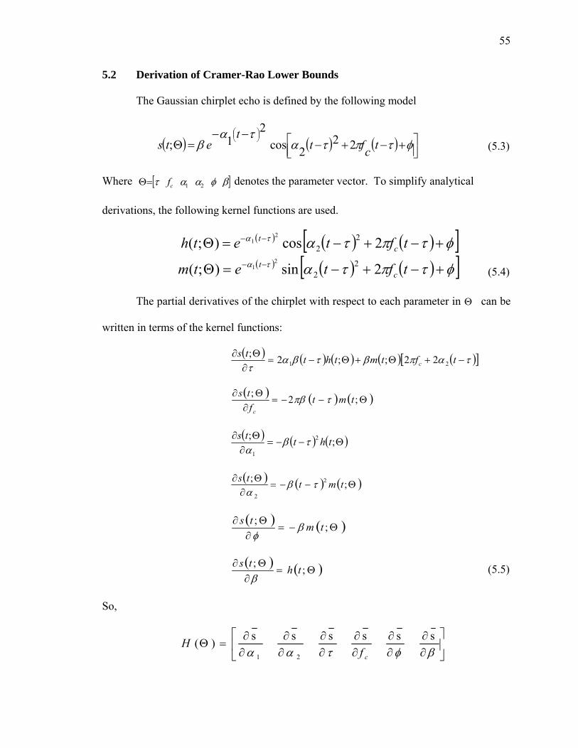
55

5.2 Derivation of Cramer-Rao Lower Bounds

The Gaussian chirplet echo is defined by the following model

( ) ( ) ( ) ⎥⎦⎤

⎢⎣⎡ +−+−

−−=Θ

⎟⎠⎞⎜

⎝⎛

φτπτατα

β tcftt

ets 222cos

21; (5.3)

Where [ ]βφαατ 21cf=Θ denotes the parameter vector. To simplify analytical

derivations, the following kernel functions are used.

( ) ( ) ( )[ ]φτπτατα +−+−=Θ −− tfteth ct 2cos);( 2

2

21

( ) ( ) ( )[ ]φτπτατα +−+−=Θ −− tftetm ct 2sin);( 2

2

21 (5.4)

The partial derivatives of the chirplet with respect to each parameter in Θ can be

written in terms of the kernel functions:

( ) ( ) ( ) ( ) ( )[ ]ταπβτβατ

−+Θ+Θ−=∂Θ∂ tftmthtts

c 21 22;;2;

( ) ( ) ( )Θ−−=∂

Θ∂ ;2; tmtfts

c

τπβ

( ) ( ) ( )Θ−−=∂

Θ∂ ;; 2

1

thtts τβα

( ) ( ) ( )Θ−−=∂

Θ∂ ;; 2

2

tmtts τβα

( ) ( )Θ−=∂

Θ∂ ;; tmts βφ

( ) ( )Θ=∂

Θ∂ ;; thtsβ

(5.5)

So,

⎥⎦

⎤⎢⎣

⎡∂∂

∂∂

∂∂

∂∂

∂∂

∂∂

=Θβφτααssssss)(

21 cfH

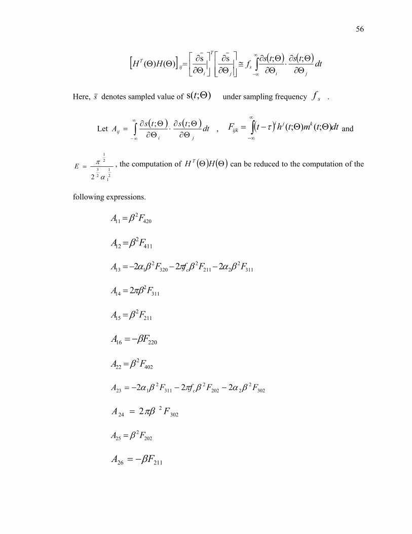
56

[ ] ( ) ( )∫∞

∞− Θ∂Θ∂

⋅Θ∂Θ∂

≅⎥⎥⎦

⎤

⎢⎢⎣

⎡

Θ∂∂

⎥⎦

⎤⎢⎣

⎡Θ∂∂

=ΘΘ dttstsfHHji

sj

T

iij

T ;;ss)()(

Here, s denotes sampled value of );s( Θt under sampling frequency sf .

Let ( ) ( )∫∞

∞− Θ∂Θ∂

⋅Θ∂Θ∂

= dttstsAji

ij;; , ( ) dttmthtF kji

ijk ∫∞

∞−

ΘΘ−= );();(τ and

21

123

21

2 α

π=E , the computation of ( ) ( )ΘΘ HH T can be reduced to the computation of the

following expressions.

4202

11 FA β=

4112

12 FA β=

3112

22112

3202

113 222 FFfFA c βαβπβα −−−=

3112

14 2 FA πβ=

2112

15 FA β=

22016 FA β−=

4022

22 FA β=

3022

22022

3112


3022

24 2 FA πβ=

2022

25 FA β=

21126 FA β−=

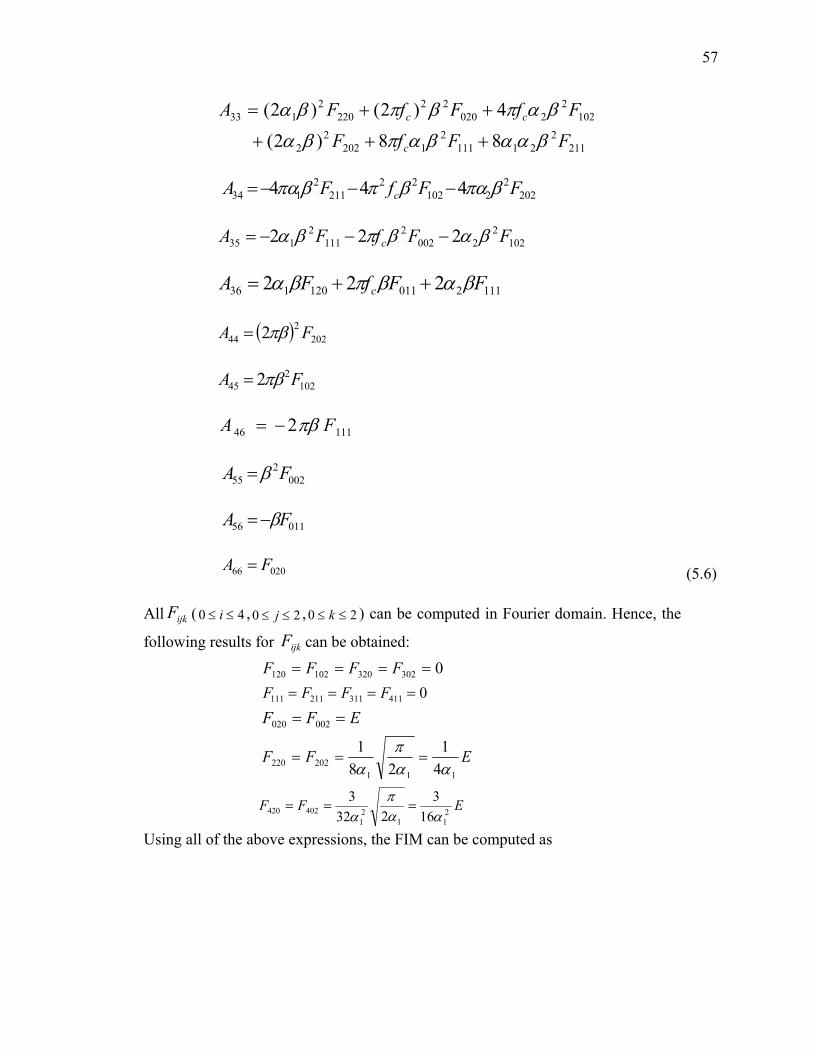
57

2112

211112

12022

2

1022

202022

2202

133

88)2(

4)2()2(

FFfF

FfFfFA

c

cc

βααβαπβα

βαπβπβα

+++

++=

2022

210222

2112

134 444 FFfFA c βπαβπβπα −−−=

1022

20022

1112


1112011120136 222 FFfFA c βαβπβα ++=

( ) 2022

44 2 FA πβ=

1022

45 2 FA πβ=

11146 2 FA πβ−=

0022

55 FA β=

01156 FA β−=

02066 FA = (5.6)

All ijkF ( 40 ≤≤ i , 20 ≤≤ j , 20 ≤≤ k ) can be computed in Fourier domain. Hence, the

following results for ijkF can be obtained:

0302320102120 ==== FFFF

0411311211111 ==== FFFF

EFF == 002020

EFF111

202220 41

281

ααπ

α===

EFF 211

21

402420 163

2323

ααπ

α===

Using all of the above expressions, the FIM can be computed as

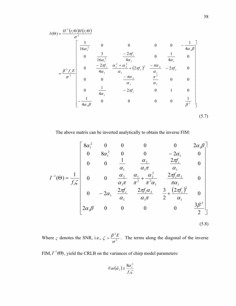
58

( ) ( )

( )

⎥⎥⎥⎥⎥⎥⎥⎥⎥⎥⎥⎥⎥⎥⎥

⎦

⎤

⎢⎢⎢⎢⎢⎢⎢⎢⎢⎢⎢⎢⎢⎢⎢

⎣

⎡

−

−

−

−−

++−

−

−

=

ΘΘ=Θ

21

1

1

2

1

2

1

22

1

22

21

1

112

1

12

1

2

2

2

100004

1

01024

10

0000

02242

0

04

1042

1630

410000

163

;;)(

ββα

πα

απ

απα

παπα

πααα

απ

ααπ

α

βαα

σβ

σ

c

ccc

c

s

T

f

fff

f

Ef

tHtHI

(5.7)

The above matrix can be inverted analytically to obtain the inverse FIM:

( )

⎥⎥⎥⎥⎥⎥⎥⎥⎥⎥⎥⎥

⎦

⎤

⎢⎢⎢⎢⎢⎢⎢⎢⎢⎢⎢⎢

⎣

⎡

+−

+

−

=Θ−

2300002

02232220

0200

02100

020080200008

1)(

2

1

1

2

1

2

11

1

2

12

22

21

1

2

11

2

1

12

1

12

1

1

ββα

απ

πααπ

απα

πααπ

απα

πα

παα

απ

παα

α

ααβαα

ζ

ccc

c

c

s

fff

f

f

fI

(5.8)

Where ζ denotes the SNR, i.e., 2

2

σβζ E

= . The terms along the diagonal of the inverse

FIM, )(1 Θ−I , yield the CRLB on the variances of chirp model parameters:

( )ζα

αsf

Var21

18ˆ ≥

59

( )ζα

αsf

Var21

28ˆ ≥

( )ζα

τsf

Var1

1ˆ ≥

( )ζαπ

αα

sc f

fVar1

2

22

21ˆ +

≥

( )( )

ζαπ

φs

c

f

f

Var 1

2223

ˆ+

≥

( )ζ

ββsf

Var23ˆ

2

≥ (5.9)

5.3 Monte Carlo Simulation

To evaluate the performance of estimation, a Monte-Carlo simulation is

performed to observe the means and variances of the estimated parameters of a single

noisy echo given in Equation 5.1. The chirp echo is simulated according to Equation 5.3

with the parameter vector listed in the Actual Parameter row of Table 5.1. The sampling

frequency is 100 MHz. The noise level is adjusted to simulate echoes with SNR levels of

20, 10 and 5 dB. For each SNR level, both algorithms (i.e., CTSD and MPSD) are

performed 250 times on the simulated chirp echo with different realizations of noise. The

average value and the variance of parameter estimators are listed in Table 5.1 along with

the analytically computed CRLB’s using Equation 5.9. One can observe that the

parameter estimation is unbiased, i.e., the mean value of the estimated parameters

achieves the actual parameter values used in simulation and the variance of estimators

attains the CRLB bounds for SNR as low as 5 dB. Therefore, the CTSD and MPSD are

60

minimum variance unbiased (MVU) estimator for a single chirp echo, hence they provide

optimal parameter estimation results.

The signal decomposition and parameter estimation algorithms significantly

improve the SNR of chirp signals. To quantify the SNR improvement, a chirp echo with

varying noise level is simulated. After estimation is performed, the output SNR (i.e., an

estimated SNR) is computed as the energy ratio of the original signal and residual error,

i.e., the difference between the original and the estimated signal. Figure 5.1 shows the

output SNR as a function of the input SNR. Each point in this plot represents a

realization of the signal with a different noise level. The parameters of the single echo

have not been changed. The input SNR has been varied from 5 dB (severely poor SNR)

to 25 dB (high SNR). It has been observed that the average SNR enhancement for the

single echo in WGN is well above 20 dB. It is important to point out that one should

expect a smaller SNR enhancement when the signal contains overlapping chirp echoes

and is corrupted correlated noise.

5.4 Observation and Analysis

In Figure 5.1a and Figure 5.1b, it can be seen that in moderate noise levels (i.e.,

input SNR varying from 10 dB to 25 dB), the estimation efficiency of MPSD algorithm is

similar, even better than that of CTSD algorithm. However, in the severe noise levels

(i.e., input SNR is below 5 dB), the MPSD algorithm is not as efficient as the CTSD

algorithm. This can be explained by the different implementation strategies of CTSD

algorithm and MPSD algorithm. First, the CTSD algorithm performs parameter

estimation in time-frequency domain whereas the MPSD algorithm performs only in time

61

domain. Hence, the noise is better suppressed in CTSD algorithm than it is in MPSD

algorithm. Secondly, the MPSD algorithm is based on iterative optimization and may

become more dependent on the initial guess in severe noise levels.

5.5 Summary

In this comparative study of chirplet model-based echo estimation techniques, two

different signal decomposition and parameter estimation algorithms (i.e., CTSD and

MPSD) are analyzed. Numerical and analytical results have shown that both algorithms

attain CRLB bounds, therefore they are robust and efficient in signal analysis.

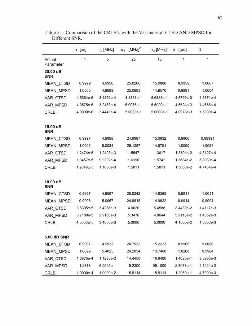
62

Table 5.1. Comparison of the CRLB’s with the Variances of CTSD AND MPSD for Different SNR.

τ [μs] ƒc [MHz] α1 [MHz]2 α2 [MHz]2 φ [rad] β

Actual Parameter

1 5 25 15 1 1

20.00 dB SNR

MEAN_CTSD 0.9999 4.9996 25.0266 15.0080 0.9959 1.0007

MEAN_MPSD 1.0000 4.9989 25.0683 14.9570 0.9991 1.0004

VAR_CTSD 4.5664e-6 3.4852e-4 4.4831e-1 5.6883e-1 4.5799e-3 1.5671e-4

VAR_MPSD 4.3575e-6 3.2463e-4 5.0075e-1 5.5020e-1 4.5524e-3 1.4666e-4

CRLB 4.0000e-6 3.4449e-4 5.0000e-1 5.0000e-1 4.0978e-3 1.5000e-4

15.00 dB SNR

MEAN_CTSD 0.9997 4.9998 24.9987 15.0932 0.9906 0.99991

MEAN_MPSD 1.0003 5.0034 25.1287 14.9751 1.0090 1.0053

VAR_CTSD 1.2474e-5 1.2403e-3 1.5547 1.3617 1.3101e-2 4.8127e-4

VAR_MPSD 1.3457e-5 9.9292e-4 1.6190 1.5742 1.3684e-2 5.3039e-4

CRLB 1.2649E-5 1.1000e-3 1.5811 1.5811 1.3000e-2 4.7434e-4

10.00 dB SNR

MEAN_CTSD 0.9997 4.9967 25.0242 14.8368 0.9911 1.0011

MEAN_MPSD 0.9998 5.0057 24.8818 14.9922 0.9914 0.9991

VAR_CTSD 3.5395e-5 3.4286e-3 4.0620 5.4588 3.4439e-2 1.4117e-3

VAR_MPSD 3.7189e-5 2.9160e-3 5.3476 4.8644 3.9118e-2 1.4352e-3

CRLB 4.0000E-5 3.4000e-3 5.0000 5.0000 4.1000e-2 1.5000e-3

5.00 dB SNR

MEAN_CTSD 0.9997 4.9933 24.7932 15.2223 0.9905 1.0080

MEAN_MPSD 1.0699 5.4025 24.2034 13.7460 1.0268 0.9984

VAR_CTSD 1.3875e-4 1.1230e-2 14.4450 16.9490 1.4020e-1 3.8953e-3

VAR_MPSD 1.2318 5.0545e-1 19.2300 95.1000 2.3073e-1 4.1424e-3

CRLB 1.0000e-4 1.0900e-2 15.8114 15.8114 1.2960e-1 4.7000e-3

63

Figure 5.1. a) Input SNR vs. Output SNR for a Single Noisy Chirp Echo Using CTSD Algorithm. b) Input SNR vs. Output SNR for a Single Noisy Chirp Echo Using MPSD Algorithm.

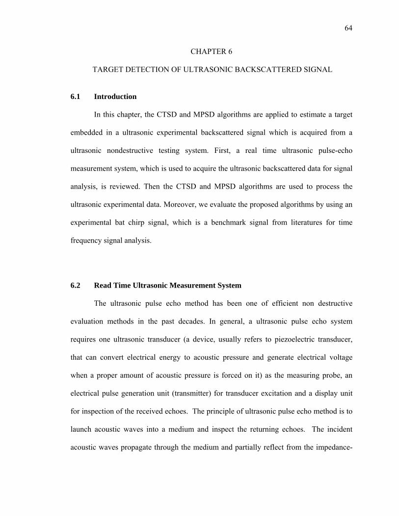
64

CHAPTER 6

TARGET DETECTION OF ULTRASONIC BACKSCATTERED SIGNAL

6.1 Introduction

In this chapter, the CTSD and MPSD algorithms are applied to estimate a target

embedded in a ultrasonic experimental backscattered signal which is acquired from a

ultrasonic nondestructive testing system. First, a real time ultrasonic pulse-echo

measurement system, which is used to acquire the ultrasonic backscattered data for signal

analysis, is reviewed. Then the CTSD and MPSD algorithms are used to process the

ultrasonic experimental data. Moreover, we evaluate the proposed algorithms by using an

experimental bat chirp signal, which is a benchmark signal from literatures for time

frequency signal analysis.

6.2 Read Time Ultrasonic Measurement System

The ultrasonic pulse echo method has been one of efficient non destructive

evaluation methods in the past decades. In general, a ultrasonic pulse echo system

requires one ultrasonic transducer (a device, usually refers to piezoelectric transducer,

that can convert electrical energy to acoustic pressure and generate electrical voltage

when a proper amount of acoustic pressure is forced on it) as the measuring probe, an

electrical pulse generation unit (transmitter) for transducer excitation and a display unit

for inspection of the received echoes. The principle of ultrasonic pulse echo method is to

launch acoustic waves into a medium and inspect the returning echoes. The incident

acoustic waves propagate through the medium and partially reflect from the impedance-

65

mismatched boundaries. The reflected acoustic waves excite the piezoelectric transducer

and form the returning ultrasonic signal.

The objective of ultrasonic pulse echo test is to evaluate the functionality and

characterization of specimen, which could be material, vegetation, or tissue texture.

Although there are a lot of information embedded in the return ultrasonic echoes, one of

the most common applications is ultrasonic target detection, which usually only addresses

the detection and positioning of defects in materials. The proposed signal decomposition

algorithms are used not only to detect and locate the targets but also enable us to

determine the characteristics of sound propagation and reflection as well as quantitatively

evaluate physical properties of targets.

The ultrasonic pulse-echo system used in this study for data acquisition is a real

time ultrasonic measurement system, which is depicted in Figure 6.1. It can be seen that

the basic elements of the system are transducer, stepper motor and controller, pulse

transmitter/receiver unit, oscilloscope with digitizer unit. The pulse transmitter/receiver

unit launches an impulse train to excite the transducer and generates a triggering signal to

control the timing of events in the system. A computer with virtual instrument

programming (i.e., LabVIEW programming) is used to control two stepper motors to

moving in both X and Y directions, and configure the sampling and digitizing parameters

for data acquisition. Due to the difficulties to reproduce the same conditions of coupling

between transducer and the specimen in transducer-contact method, we use water as

couplant in this experiment and immerse the specimen and transducer in a water tank.

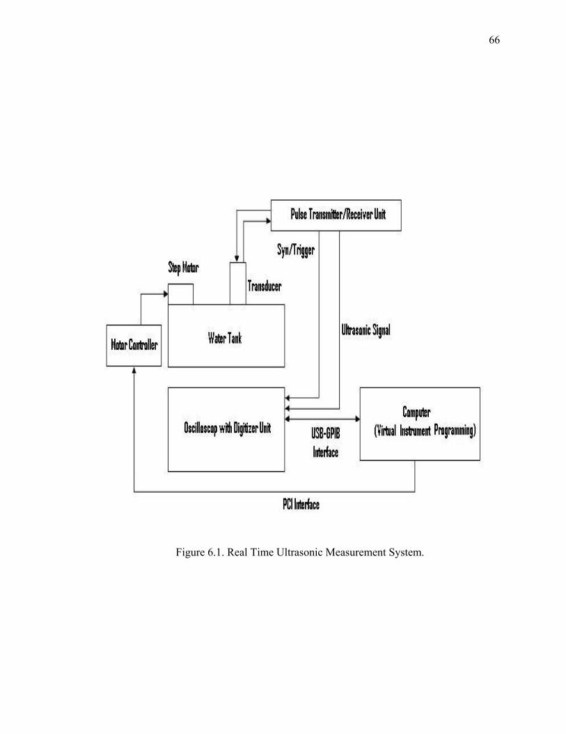
66

Figure 6.1. Real Time Ultrasonic Measurement System.

67

According to the transducer scan mode, there exist different testing procedures

(i.e., A-scan, B-scan and C-scan). When the transmitted signal scans the specimen along

the transducer axis through one fixed point, the acquired data is called A-scan (Amplitude

scan). When the transducer is moved along X or Y direction, it yields 2-D image, which

is called B-scan (Brightness scan). When the transducer is moved both in X and Y

directions, it would yields 3-D image. The image slice perpendicular to the transducer

axis is called C-scan (Constant depth scan). It can be seen that the A-scan is the base of

B-scan and C-scan. The quality of B-scan and C-scan in turn depend on the quality of A-

scan data in certain extent. The accurate analysis and enhancement of A-scan can

improve B-scan and C-scan for ultrasonic imaging and further process. The signal

decomposition algorithms aim to efficiently analysis an A-scan data.

6.3 Target Detection in Ultrasonic Backscattered Signal

The CTSD algorithm is utilized to evaluate an ultrasonic experimental

backscattered signal consisting of many interfering echoes and detect a embedded target.

The experimental signal is acquired from a steel block with a flat-bottom hole (i.e., target)

using a nominal center frequency 5MHz transducer and sampling rate of 100 MHz.

Figure 6.2 shows the reconstructed signal using CTSD algorithm (dash line)

superimposed the experimental ultrasonic backscattered echoes (solid line). The

experimental signal has poor SNR and the target echo shows interference from

microstructure scattering and measurement noise. The reconstructed signal and its

chirplet transform representation are shown in Figure 6.3c and Figure 6.3d. The

parameters of each decomposed chirplet using CTSD algorithm are listed in the Table 6.1.

68

Furthermore, the comparison between the experimental signal and the reconstructed

signal using CTSD algorithm (see Figure 6.2 and Figure 6.3) clearly demonstrates that

the chirplet signal decomposition has been successful in estimating echoes and filtering

out the noise.

Similarly, the MPSD algorithm is evaluated using the same ultrasonic

experimental backscattered signal consisting of many interfering echoes to detect the

embedded target. Figure 6.4 shows the reconstructed signal (dash line) using MPSD

algorithm superimposed the experimental ultrasonic backscattered echoes (solid line).

The experimental signal has poor SNR and the target echo shows interference from

microstructure scattering and measurement noise. The WVD representation of the

experimental signal (see Figure 6.5b) clearly shows that the experimental signal has poor

SNR and the target echo is completely embedded in the interference from microstructure

scattering, measurement noise. The cross-term effect of WVD also smears the target

information in the time frequency representation. After the process of decomposition, the

reconstructed signal and its WVD representation are shown in Figure 6.5c and Figure

6.5d. The parameters of each decomposed chirplet using MPSD algorithm are listed in

the Table 6.2. The comparison between the experimental signal and the reconstructed

signal using MPSD algorithm (see Figure 6.4 and Figure 6.5) also clearly demonstrates

that the decomposition has been successful in detecting the target echo and filtering out

the noise.

From the discussion of ultrasonic target detection, it can be seen that the CTSD

and MPSD algorithm can decompose and reconstruct the heavily overlapped ultrasonic

backscattered signal with high accuracy. The time frequency representations show that

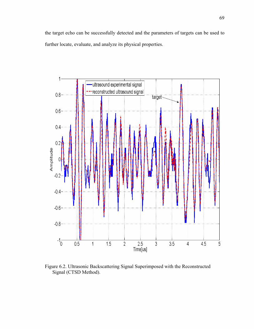
69

the target echo can be successfully detected and the parameters of targets can be used to

further locate, evaluate, and analyze its physical properties.

Figure 6.2. Ultrasonic Backscattering Signal Superimposed with the Reconstructed Signal (CTSD Method).

70

Figure 6.3. a) Ultrasonic Backscattering Signal. b) TF Representation of the Ultrasonic Backscattered Signal. c) Estimated Signal.d) TF representation of the Estimated Signal.

71

Table 6.1 Parameter Estimation Results for Ultrasonic signal (CTSD)


1 0.5308 4.7014 43.0777 3.4705 0.8524 0.9276

2 1.2283 4.8446 308.7686 427.96 4.7114 0.8536

3 3.8402 3.3447 31.253 -22.8812 1.1696 0.8437

4 0.6605 3.7696 222.0866 90.9201 5.0828 0.6972

5 4.9418 5.6884 62.9997 8.5722 6.0407 0.5471

6 4.7969 4.0229 324.299 -85.4654 0.9936 0.5387

7 4.179 4.5125 93.1408 -15.737 2.1609 0.5046

8 4.3933 5.2119 48.4645 -3.5827 3.1171 0.4987

9 3.1771 5.8968 38.5415 27.8241 1.1234 0.487

10 1.3715 4.8725 155.1614 -172.874 4.0749 0.4794

11 1.8503 5.7028 70.8195 49.3017 4.8279 0.4581

12 2.527 5.2801 43.2308 -22.0839 1.6656 0.3998

13 -0.3449 10.6442 3.6708 -39.8702 5.033 0.3621

14 2.1343 6.5791 137.6486 114.295 4.883 0.3415

15 0.9926 5.9012 24.035 69.3318 0.4228 0.3295

16 1.5421 4.403 16.1625 -34.1705 2.7274 0.2961

17 3.4903 3.7745 33.1804 -51.7901 0.9032 0.1901

18 2.7452 3.9808 34.1805 -43.3182 2.0305 0.1656

72

Figure 6.4. Ultrasonic Backscattering Signal Superimposed with the Reconstructed Signal (MPSD Method).

73

Figure 6.5. a) Ultrasonic Backscattering Signal. b) WVD of Ultrasonic Backscattering Signal. c) the Reconstructed Signal d) WVD of the Reconstructed Signal Using MPSD Method.

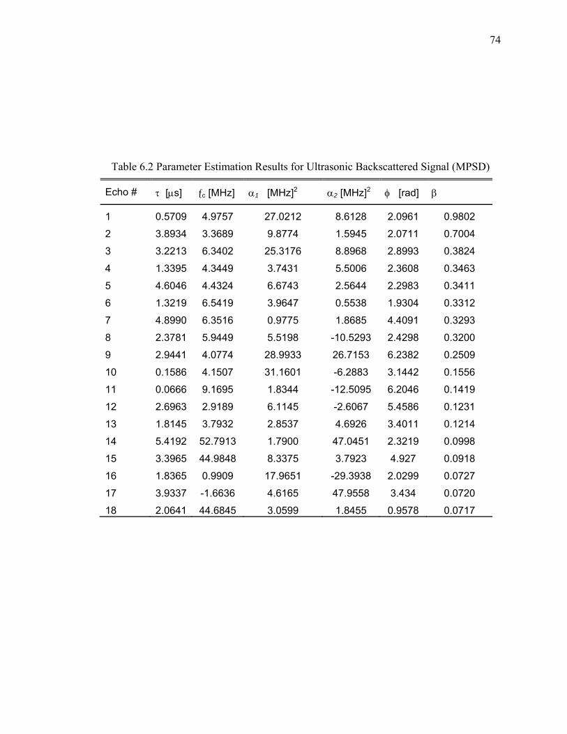
74

Table 6.2 Parameter Estimation Results for Ultrasonic Backscattered Signal (MPSD)


1 0.5709 4.9757 27.0212 8.6128 2.0961 0.9802

2 3.8934 3.3689 9.8774 1.5945 2.0711 0.7004

3 3.2213 6.3402 25.3176 8.8968 2.8993 0.3824

4 1.3395 4.3449 3.7431 5.5006 2.3608 0.3463

5 4.6046 4.4324 6.6743 2.5644 2.2983 0.3411

6 1.3219 6.5419 3.9647 0.5538 1.9304 0.3312

7 4.8990 6.3516 0.9775 1.8685 4.4091 0.3293

8 2.3781 5.9449 5.5198 -10.5293 2.4298 0.3200

9 2.9441 4.0774 28.9933 26.7153 6.2382 0.2509

10 0.1586 4.1507 31.1601 -6.2883 3.1442 0.1556

11 0.0666 9.1695 1.8344 -12.5095 6.2046 0.1419

12 2.6963 2.9189 6.1145 -2.6067 5.4586 0.1231

13 1.8145 3.7932 2.8537 4.6926 3.4011 0.1214

14 5.4192 52.7913 1.7900 47.0451 2.3219 0.0998

15 3.3965 44.9848 8.3375 3.7923 4.927 0.0918

16 1.8365 0.9909 17.9651 -29.3938 2.0299 0.0727

17 3.9337 -1.6636 4.6165 47.9558 3.434 0.0720

18 2.0641 44.6845 3.0599 1.8455 0.9578 0.0717

75

6.4 Bat Chirp Signal Analysis

Bat is one of species that use ultrasound for echolocation. The research of its

sound is important in scientific research, which providing insights into the biology of

hibernation and sonar mechanisms. There is an experimental chirp data which is emitted

by a large brown bat in the signal analysis literatures [Qia98, Fen01, Wan01, Cap03,

Rub05, and Don06]. It has been used as a benchmark signal for time frequency signal

analysis. Thanks to Beckman Institute, University of Illinois for offering the data, we can

evaluate the proposed signal decomposition algorithms using the bat chirp signal.

The CTSD algorithm is applied to process the bat chirp signal emitted by the large

brown bat, which is digitized within 2.2 ms duration with sampling period of 7 us. Figure

6.6 shows the reconstructed signal using CTSD algorithm (dash line) superimposed the

experimental bat chirp signal (solid line). The parameters of each decomposed chirplet

using CTSD algorithm are listed in the Table 6.3. The bat chirp signal has poor SNR and

contains heavily overlapping chirp components. From the reconstructed signal and its

chirplet transform representation (shown in Figure 6.7c and Figure 6.7d), it can be seen

that the bat chirp signal includes three main stripes. These stripes are highly overlapped

with each other in both time domain and frequency domain, which add the difficulties for

signal analysis. The process results (shown in Figure 6.6, Figure 6.7 and Table 6.3)

clearly demonstrate that the chirplet signal decomposition not only successful analyzes

the contents of bat echoes as the other literatures did, but offer the details of parameters

for better scientific analysis of the species.

Similarly, the MPSD algorithm is evaluated using the same experimental bat chirp

echoes. Figure 6.8 shows the reconstructed signal (dash line) using MPSD algorithm

76

superimposed the experimental bat chirp echoes (solid line). . The parameters of each

decomposed chirplet using MPSD algorithm are listed in the Table 6.4. The WVD

representation of the experimental bat chirp echoes (see Figure 6.9b) shows that the cross

term effect of WVD conceals the characteristics of bat signal. After the process of

MPSD algorithm, the WVD representation of the reconstructed signal (see Figure 6.9d)

suppresses the cross terms and reveals the similar three main stripes in time frequency

domain. The process results (shown in Figure 6.8, Figure 6.9 and Table 6.4) show the

decomposition with high efficiency in the bat chirp signal analysis.

6.5 Summary

In this chapter, the CTSD and MPSD algorithm has been evaluated in the

ultrasonic target detection and bat chirp signal analysis. Experimental results and

performance analysis indicate the robustness of the proposed algorithms in these

applications.

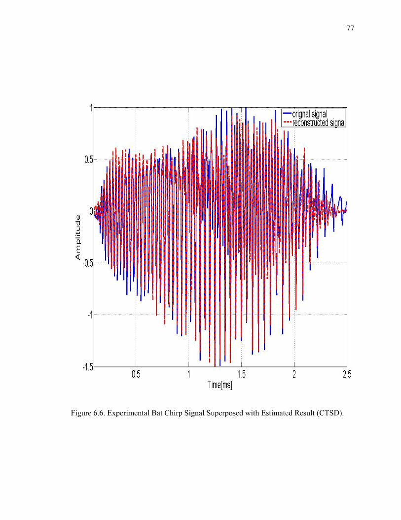
77

Figure 6.6. Experimental Bat Chirp Signal Superposed with Estimated Result (CTSD).

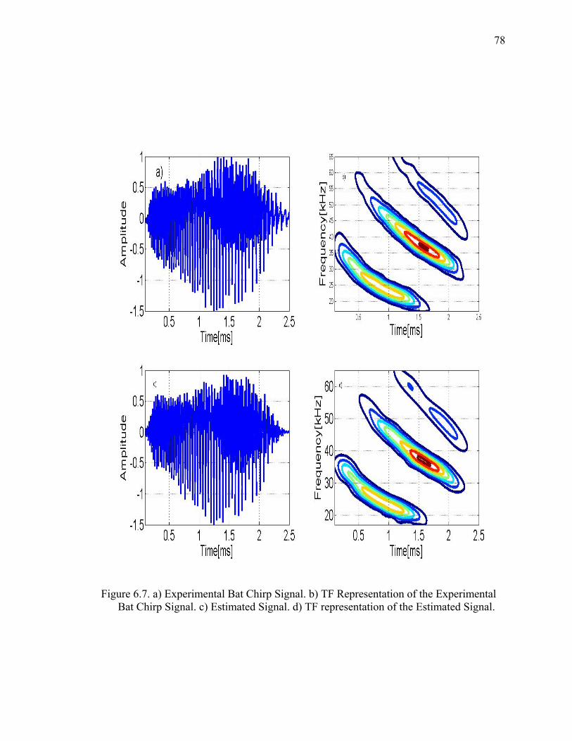
78

Figure 6.7. a) Experimental Bat Chirp Signal. b) TF Representation of the Experimental Bat Chirp Signal. c) Estimated Signal. d) TF representation of the Estimated Signal.

79

Table 6.3. Parameter Estimation Results for Bat Chirp (CTSD)

Echo # τ [μs] ƒc [KHz] α1 [KHz]2 α2 [KHz]2 φ [rad] β

1 1.60 36.9 5.8 -39.7 -2.07 0.995

2 1.20 20.3 16.4 -15.5 2.29 0.830

3 .819 25.0 6.0 -45.4 -1.53 0.761

4 1.10 44.4 37.1 -55.8 -1.1 0.724

5 .854 24.4 12.1 -51.1 0.81 0.723

6 .910 24.0 4.10 -39.2 -0.14 0.646

7 .287 33.9 76.4 -58.9 1.1 0.633

8 1.00 21.2 60.7 -15.6 0.46 0.425

9 .777 50.6 14.4 -87.5 -0.87 0.330

10 2.00 32.0 29.2 -55.9 -1.79 0.313

11 1.80 51.2 6.2 -64.8 -0.83 0.297

12 1.30 60.8 15.1 -62.4 -2.36 0.254

13 2.10 44.3 16.8 -81.9 -1.88 0.168

14 2.00 62.9 68.5 -34.5 1.49 0.155

15 1.30 41.3 194.7 -26.0 -2.53 0.134

16 .917 71.4 51.6 63.7 2.87 0.120

17 1.60 36.0 33.5 -19.3 -2.04 0.120

18 1.70 71.4 27.6 70.2 2.68 0.096

80

Figure 6.8. Experimental Bat Chirp Signal Superposed with Estimated Result (MPSD).

81

Figure 6.9 a) Bat Chirp Signal. b) WVD of Bat Chirp Signal. c) the Reconstructed Signal d) WVD of the Reconstructed Signal Using MPSD Method.

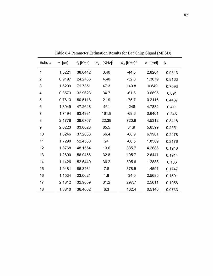
82

Table 6.4 Parameter Estimation Results for Bat Chirp Signal (MPSD)

Echo # τ [μs] ƒc [KHz] α1 [KHz]2 α2 [KHz]2 φ [rad] β

1 1.5221 38.0442 3.40 -44.5 2.8264 0.9643

2 0.9197 24.2786 4.40 -32.8 1.3079 0.8163

3 1.6299 71.7351 47.3 140.8 0.849 0.7093

4 0.3573 32.9623 34.7 -61.6 3.6695 0.691

5 0.7813 50.5118 21.9 -75.7 0.2116 0.4437

6 1.3949 47.2648 464 -248 4.7882 0.411

7 1.7494 63.4931 161.8 -69.6 0.6401 0.345

8 2.1776 38.6767 22.39 720.9 4.5312 0.3418

9 2.0223 33.0028 85.5 34.9 5.6599 0.2551

10 1.6246 37.2038 66.4 -68.9 6.1901 0.2478

11 1.7290 52.4530 24 -66.5 1.8509 0.2176

12 1.8768 48.1554 13.6 335.7 4.2686 0.1948

13 1.2600 56.9456 32.8 105.7 2.6441 0.1914

14 1.1426 52.6449 36.2 595.6 1.2888 0.186

15 1.9481 86.3461 7.8 378.5 1.4591 0.1747

16 1.1534 23.0621 1.8 -34.0 2.5685 0.1501

17 2.1812 32.9059 31.2 297.7 2.5611 0.1056

18 1.8810 36.4662 6.3 162.4 0.5146 0.0733

83

CHAPTER 7

STATISTICAL EVALUATION USING ULTRASONIC GRAIN SIGNAL

7.1 Introduction

In polycrystalline materials, almost all the important mechanical properties of

materials, such as strength, hardness, elasticity and magnetic characteristics, depend on

their grain size. Hence the grain size estimation is critical for material evaluation.

Intercept method is a simple method of grain size measurement. The method counts the

number of grain boundaries intersected by a test line and provides an average intercept

length to match ASTM (American Society for Testing and Materials) grain size number.

The most advantages of this method are its simple interpretation and high computational

efficiency. However, the process to take microscopic examination of the material is slow,

which is not amenable to on-line application and the count of grain number is subjective.

A considerable effort has been directed to estimate grain size by using ultrasonic

backscattered grain signals. More recently, the homomorphic processing, low-order

autoregressive models, and neural network have been applied to ultrasonic backscattered

signals for grain sizing [San89, Wan91].

This chapter presents the application of CTSD algorithm in grain size estimation.

First, a frequency-dependent statistical model of ultrasound backscattered grain echoes is

addressed [San81, Wan91]. Through the analysis of this model, the connection between

frequency shift trends of grain echoes with the average grain size of materials is revealed.

Furthermore, as an alternative technique of material evaluation, the proposed CTSD

algorithm is used to decompose the ultrasonic experimental backscattered echoes, which

are measured from different samples with different average grain size, into chirplets.

84

Then, the estimated parameters of chirplets are used to evaluate the average grain size of

specimens.

7.2 Ultrasonic Backscattered Model

Based on the fact that the ultrasonic wave traveling through materials undergoes

energy loss due to absorption and scattering, The amplitude of the backscattered

signal, bA , can be modeled as [San89]

∫=

∫=

−

+−

z

zas

dzfz

s

dzfzfz

sb

efzA

efzAA

0

0

),(2

0

)),(),((2

0

),(

),(α

αα

α

α (7.1)

Where 0A denotes the initial amplitude, ),( fzsα denotes the scattering coefficient,

which is depend on position, z , and frequency , f . Similarly, ),( fzaα denotes the

absorption coefficient, and ),( fzα denotes the overall attenuation coefficient, which is

the combination coefficient of absorption and scattering. If the materials exhibit

homogeneous properties as a function of position z , then the Equation 7.1 can be

simplified to

zfsb efAA )(2

0 )( αα −= (7.2)

In general, grain scattering losses are larger compared to absorption losses. The

scattering formulas have been intensively studied and classified into distinct scattering

regions based on the ratio of sound wavelength, λ , to the mean grain diameter,

D [San89]. The scattering regions are tabulated in Table 7.1. In Rayleigh scattering

region, where the ultrasound wavelength is much greater than the mean grain diameter,

85

the scattering coefficient varies with the average volume of the grain ( 3D ) and the

fourth power of ultrasonic wave frequency, while absorption increases linearly with

frequency. Since Rayleigh scattering )( fsα shows high sensitivity to the variation in

grain size and frequency, the Rayleigh scattering region will be of our primary concern.

The attenuation coefficient can be represented in terms of the grain size and frequency

4321)( fDff ααα += (7.3)

Where 1α denotes the absorption constant, 2α is the scattering constant, and f denotes

the wave frequency. In the Rayleigh scattering region, the scattering coefficient )( fsα

is a function of frequency ( λDf ∝ ) [San81]. High frequency components exhibit

larger intensity in backscattered echoes compared with the low frequency components.

Consequently, this situation results in an upward shift in the expected frequency of the

power spectrum corresponding to the broadband echoes. Since the spectral shift is grain

size dependent, the estimate of the upward shift can be used for grain size

characterization. Furthermore, from the Equation 7.2 it can be seen that the term

zfe )(2α− influences the frequency shift in a downward direction. The downward shift is

dependent on the position of the scatters relative to the transmitting/receiving transducer.

The two opposing phenomena (i.e., upward shift due to scattering and downward shift

caused by attenuation) can potentially be used grain size evaluation. Estimating the

frequency shift can be achieved from random patterns of grain echoes, which is a

challenging task.

86

Table 7.1 Scattering Coefficients as a Function of Mean Grain Diameter and Frequency.

Scattering region Scattering function Relationships

Rayleigh 431 fDC D>>λ

Stochastic 22 fDC D≈λ

Diffusive

DC3 D<<λ

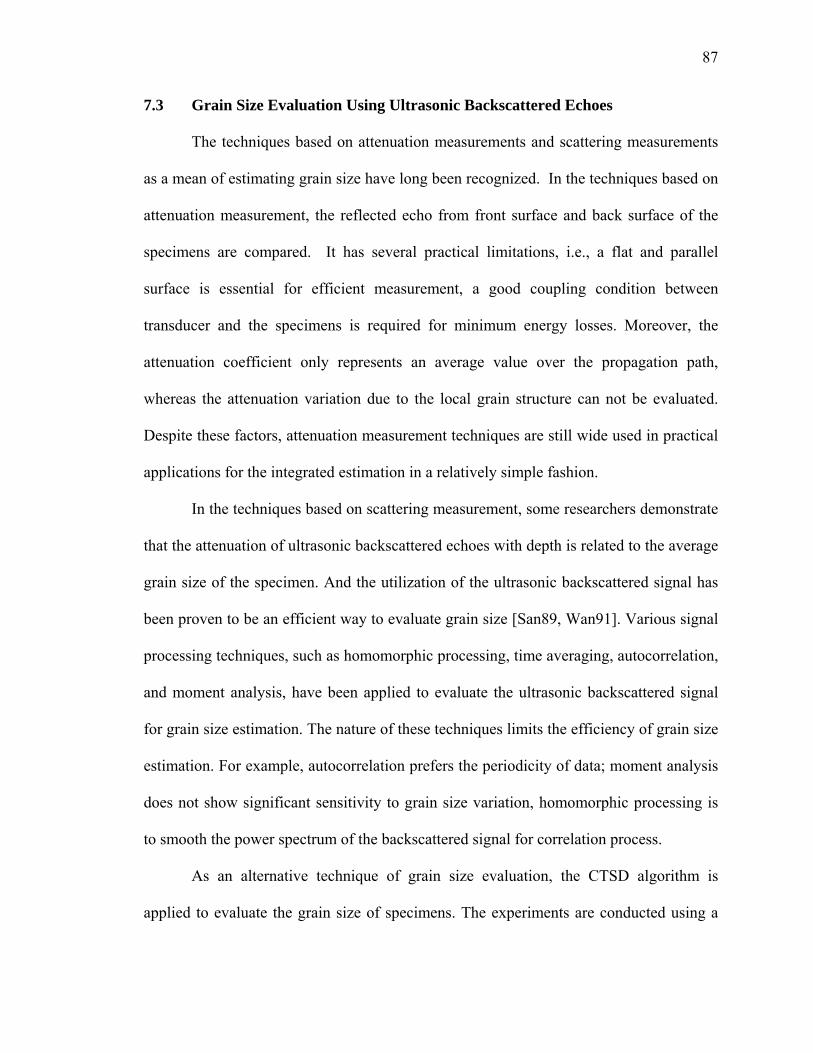
87

7.3 Grain Size Evaluation Using Ultrasonic Backscattered Echoes

The techniques based on attenuation measurements and scattering measurements

as a mean of estimating grain size have long been recognized. In the techniques based on

attenuation measurement, the reflected echo from front surface and back surface of the

specimens are compared. It has several practical limitations, i.e., a flat and parallel

surface is essential for efficient measurement, a good coupling condition between

transducer and the specimens is required for minimum energy losses. Moreover, the

attenuation coefficient only represents an average value over the propagation path,

whereas the attenuation variation due to the local grain structure can not be evaluated.

Despite these factors, attenuation measurement techniques are still wide used in practical

applications for the integrated estimation in a relatively simple fashion.

In the techniques based on scattering measurement, some researchers demonstrate

that the attenuation of ultrasonic backscattered echoes with depth is related to the average

grain size of the specimen. And the utilization of the ultrasonic backscattered signal has

been proven to be an efficient way to evaluate grain size [San89, Wan91]. Various signal

processing techniques, such as homomorphic processing, time averaging, autocorrelation,

and moment analysis, have been applied to evaluate the ultrasonic backscattered signal

for grain size estimation. The nature of these techniques limits the efficiency of grain size

estimation. For example, autocorrelation prefers the periodicity of data; moment analysis

does not show significant sensitivity to grain size variation, homomorphic processing is

to smooth the power spectrum of the backscattered signal for correlation process.

As an alternative technique of grain size evaluation, the CTSD algorithm is

applied to evaluate the grain size of specimens. The experiments are conducted using a

88

Panametrics transducer A3062 with nominal center frequency 5 MHz with sampling rate

100 MHz. Steel blocks with different grain sizes were examined. The different structures

and correspondingly different grains in specimens are often obtained by using different

heat treatments. In our experiment, the grain size of reference sample (without heat

treatment) is 14 μm. Two of steel blocks were annealed at 1600oF and 1900oF for 4 hours

heat, then air cooled to room temperature, that increased the average grain size to 24 μm

and 50 μm, respectively. The micrographs with 400 magnifications of all three specimens

are shown in Figure 7.1.

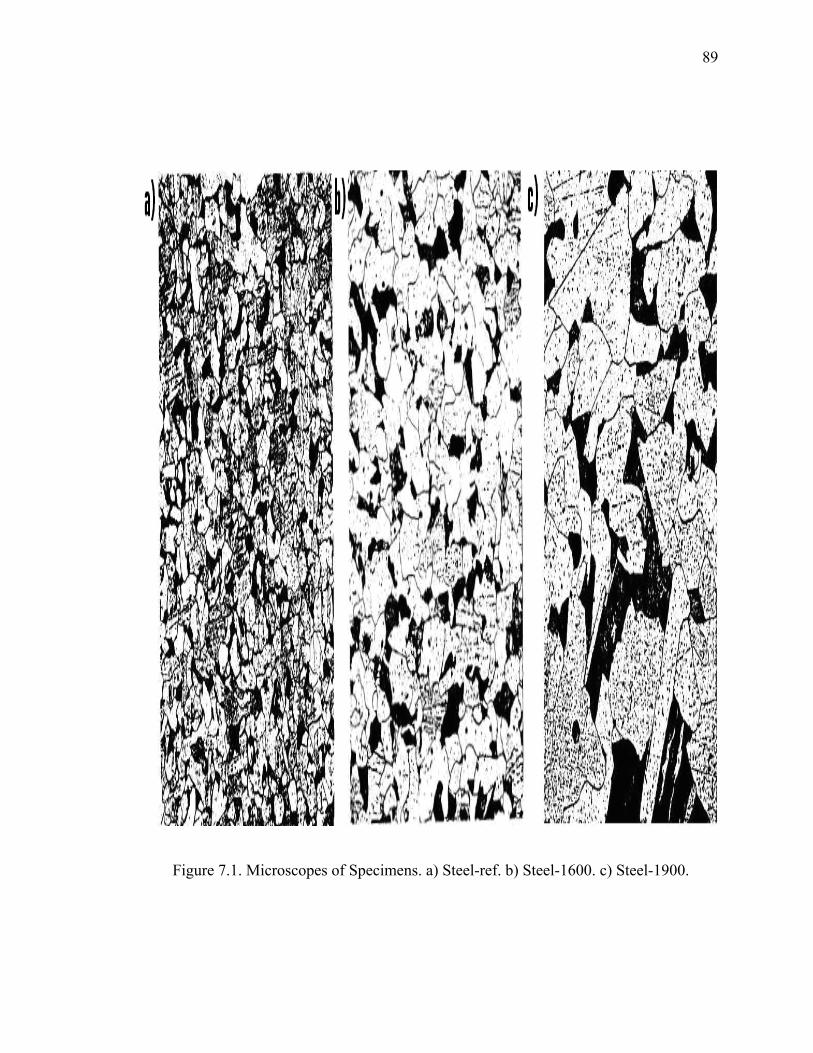
89

Figure 7.1. Microscopes of Specimens. a) Steel-ref. b) Steel-1600. c) Steel-1900.

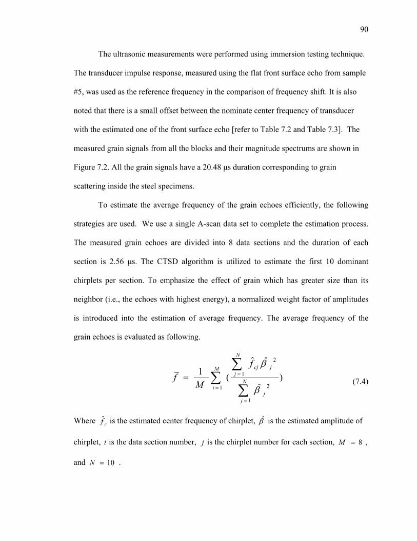
90

The ultrasonic measurements were performed using immersion testing technique.

The transducer impulse response, measured using the flat front surface echo from sample

#5, was used as the reference frequency in the comparison of frequency shift. It is also

noted that there is a small offset between the nominate center frequency of transducer

with the estimated one of the front surface echo [refer to Table 7.2 and Table 7.3]. The

measured grain signals from all the blocks and their magnitude spectrums are shown in

Figure 7.2. All the grain signals have a 20.48 μs duration corresponding to grain

scattering inside the steel specimens.

To estimate the average frequency of the grain echoes efficiently, the following

strategies are used. We use a single A-scan data set to complete the estimation process.

The measured grain echoes are divided into 8 data sections and the duration of each

section is 2.56 μs. The CTSD algorithm is utilized to estimate the first 10 dominant

chirplets per section. To emphasize the effect of grain which has greater size than its

neighbor (i.e., the echoes with highest energy), a normalized weight factor of amplitudes

is introduced into the estimation of average frequency. The average frequency of the

grain echoes is evaluated as following.

∑∑

∑=

=

==M

iN

jj

N

jjcjf

Mf

1

1

2

1

2

)ˆ

ˆˆ

(1

β

β

(7.4)

Where cf̂ is the estimated center frequency of chirplet, β̂ is the estimated amplitude of

chirplet, i is the data section number, j is the chirplet number for each section, 8=M ,

and 10=N .

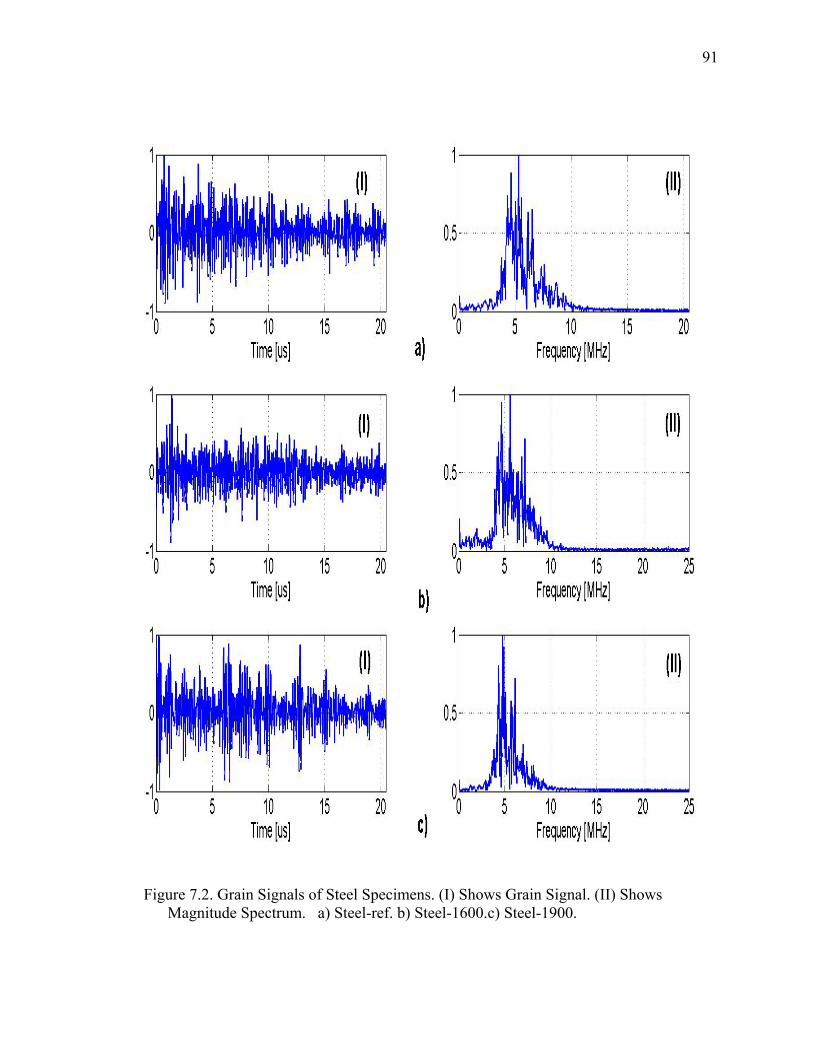
91

Figure 7.2. Grain Signals of Steel Specimens. (I) Shows Grain Signal. (II) Shows Magnitude Spectrum. a) Steel-ref. b) Steel-1600.c) Steel-1900.

92

As discussed in Section 7.2, there is an inherent upward shift in the frequency of

the grain echoes due to scattering, and a downward shift caused by the attenuation effect.

In all the measured grain signals, it was observed that the upward shift in the frequency is

far more dominating than the downward shift. The quantitative center frequencies of

grains are presented in the Table 7.2. As shown in the table, all specimens exhibit an

upward shift in the frequency due to the scattering effect compared to reference echo.

However, since attenuation begins to dominate as the grain size increases, the degree of

upward shift is reduced with respect to the reference signal for larger grained samples.

Fox example, steel-1900(the specimen with the largest grains) shows a lower upward

frequency shift than the other two samples. Note that steel-1600 shows a slightly higher

upward frequency shift in the estimated frequency than the steel-ref specimen, which is in

consistent with the model prediction. This discrepancy may be caused by the estimation

error and/or possible inherent variations in the scattering properties of the grains. It is

important to point out that the quantitative relationship between the average grain size

and the expected frequency shift is dependent on the type of material, the quality of grain

boundaries, as well as the characteristics of the measuring instruments. Therefore, proper

interpretation of the presence or absence of frequency shift in the measured data needs to

be carefully examined prior to its application to grain size characterization.

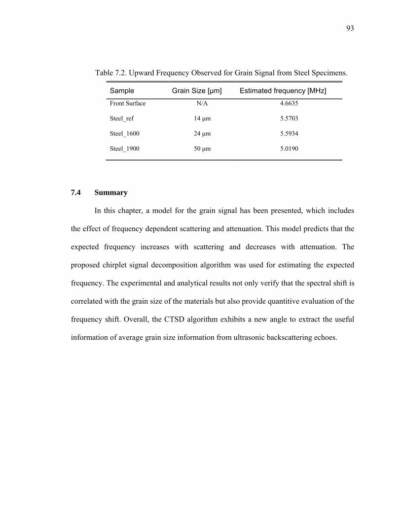
93

Table 7.2. Upward Frequency Observed for Grain Signal from Steel Specimens.

Sample Grain Size [μm] Estimated frequency [MHz]

Front Surface N/A 4.6635

Steel_ref 14 μm 5.5703

Steel_1600 24 μm 5.5934

Steel_1900 50 μm 5.0190

7.4 Summary

In this chapter, a model for the grain signal has been presented, which includes

the effect of frequency dependent scattering and attenuation. This model predicts that the

expected frequency increases with scattering and decreases with attenuation. The

proposed chirplet signal decomposition algorithm was used for estimating the expected

frequency. The experimental and analytical results not only verify that the spectral shift is

correlated with the grain size of the materials but also provide quantitive evaluation of the

frequency shift. Overall, the CTSD algorithm exhibits a new angle to extract the useful

information of average grain size information from ultrasonic backscattering echoes.

94

CHAPTER 8

ULTRASONIC REVERBERANT APPLICATION

8.1 Introduction

In ultrasonic imaging applications, the problem of reverberating patterns arises

frequently. The reverberant echoes which comprise the entire signal complicate the

characterization of objects. For example, in medical imaging system, the multiple

reflection produced by reverberations in the bone become the dominant feature and

obscure signals from surrounding tissue. In ultrasonic non-destructive material evaluation

applications, the reverberant patterns usually occur in the measurement of thin planar

defects in metal, lamination of composite bonds, gap thickness measurements of metal

adhesively bonded system, and fatigue crack analysis, etc. A theoretical model was

successfully developed to characterize the multilayered reverberant environment that

exists in the detection of corrosion or volatile changes in the steam generator tubing

system [San89].

In this chapter, The CTSD algorithm application in ultrasonic multilayered

reverberant structure is presented. First, a theoretical reverberation model is reviewed.

The model describes the reverberation phenomenon for multilayered structures and

provides critical insight in the characterization of boundaries of multilayered structures.

Then, the proposed CTSD algorithm is utilized to analyze an experimental reverberant

signal from multilayered structures. The physical properties of the multilayered

structures are appropriately interpreted by the estimated parameters of chirplets.

95

8.2 Reverberant Signal Model for Multilayered Structures

For the sake of developing a theoretical base of analyzing the backscattered

echoes from a highly reverberant discrete structure, the case of a single thin layer is

examined first. Figure 8.1 illustrates an outline of the reverberation process which shows

the normal incident beam and the corresponding transmitted and reflected beams as a

function of time, where region I , region II, and region III are defined by their density ,

and the velocity of sound in that media. The incident ultrasonic beam impinging the thin

layer is partially reflected and transmitted at each boundary as shown in Figure 8.1. Using

the characteristic impedances, the reflection and transmission coefficients of each

boundary can be calculated using

ji

jiij ZZ

ZZ+−

=α and ji

iij ZZ

Z+

=2β (8.1)

Where ijα and ijβ are the reflection and transmission coefficients of adjacent regions i

and j , respectively.

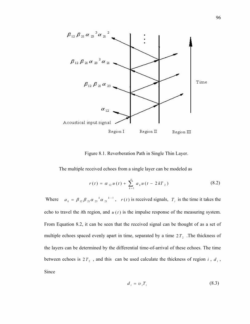
96

Figure 8.1. Reverberation Path in Single Thin Layer.

The multiple received echoes from a single layer can be modeled as

∑∞

=

−+=1

212 )2()()(k

k kTtuatutr α (8.2)

Where 121232112

−= kkka ααββ , )( tr is received signals, iT is the time it takes the

echo to travel the ith region, and )( tu is the impulse response of the measuring system.

From Equation 8.2, it can be seen that the received signal can be thought of as a set of

multiple echoes spaced evenly apart in time, separated by a time 22T .The thickness of

the layers can be determined by the differential time-of-arrival of these echoes. The time

between echoes is 22 T , and this can be used calculate the thickness of region i , id ,

Since

iii Td υ= (8.3)

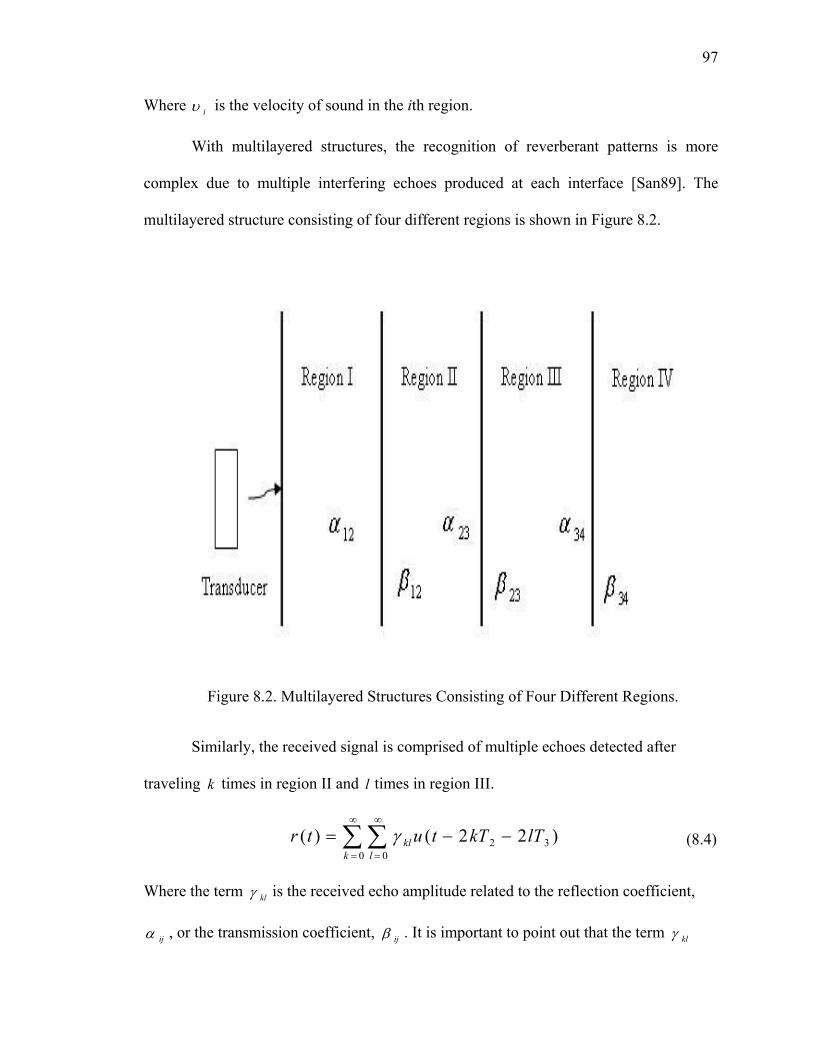
97

Where iυ is the velocity of sound in the ith region.

With multilayered structures, the recognition of reverberant patterns is more

complex due to multiple interfering echoes produced at each interface [San89]. The

multilayered structure consisting of four different regions is shown in Figure 8.2.

Figure 8.2. Multilayered Structures Consisting of Four Different Regions.

Similarly, the received signal is comprised of multiple echoes detected after

traveling k times in region II and l times in region III.

∑∑∞

=

∞

=

−−=0 0

32 )22()(k l

kl lTkTtutr γ (8.4)

Where the term klγ is the received echo amplitude related to the reflection coefficient,

ijα , or the transmission coefficient, ijβ . It is important to point out that the term klγ

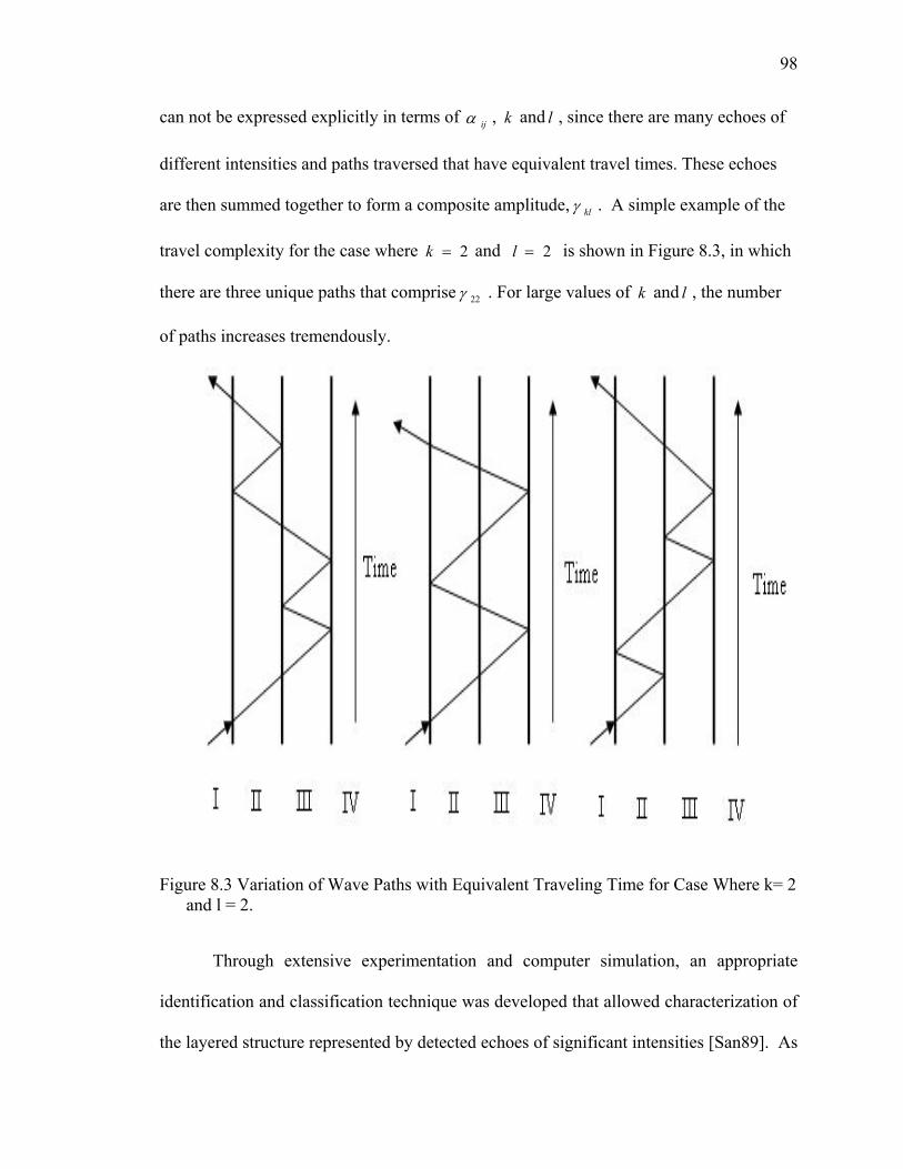
98

can not be expressed explicitly in terms of ijα , k and l , since there are many echoes of

different intensities and paths traversed that have equivalent travel times. These echoes

are then summed together to form a composite amplitude, klγ . A simple example of the

travel complexity for the case where 2=k and 2=l is shown in Figure 8.3, in which

there are three unique paths that comprise 22γ . For large values of k and l , the number

of paths increases tremendously.

Figure 8.3 Variation of Wave Paths with Equivalent Traveling Time for Case Where k= 2 and l = 2.

Through extensive experimentation and computer simulation, an appropriate

identification and classification technique was developed that allowed characterization of

the layered structure represented by detected echoes of significant intensities [San89]. As

99

a result of classification the generalized model for the received echoes given in Equation

8.4 can be re-organized differently:

⋅⋅⋅+−−+

−−+

−+=

∑

∑

∑

∞

=

∞

=

∞

=

023

123

1212

)24(

)22(

)2()()(

kk

kk

kk

kTTtuc

kTTtub

kTtuatutr α

(8.5)

Where ka is the amplitude of the class “a” echoes, which reverberate in region II only;

kb is the amplitude of the class “b” echoes, which reverberate continually in region II

and once in region III; kc is the amplitude of the class “c” echoes, which reverberate

continually in region II and twice in region III; etc.

The amplitude of these classes of echoes has explicitly close-forms:

kk Aa 0

21

2112 )(αββ

= ; for 1≥k

101

21

2112 )( −= kk AAkb

αββ

for 1≥k

221

21121 Ac

αββ

=

⎥⎦⎤

⎢⎣⎡ −

+= −− 20

21

102

21

2112

21)( kk

k AAkAAkcαββ

for 1>k

where 211

32343223 αααββ −= nnnA . (8.6)

The amplitude of echo pulse 1+ka is less than that of ka due to energy loss at

the boundary of region II. Each time the incident sound reaches the back surface of

100

region II, a small fraction of it passes into the water gap (region III) and reverberates

between adjacent region II and region IV. Each time a sound packet returns to region II, a

small fraction of its energy is transmitted through it toward the transducer. Each time the

“a” type wave packet reaches the back surface of region II it generates a water gap wave

packet which, upon returning to the region, adds energy to the “b” series of signals. Thus

the class “a” pulses decrease with time whereas the “b” series should actually increase

with time, at least until it in turn loses energy to a “c” type wave train. Class “c” echoes

consist of region II reverberations which have traversed region II twice. However,

because such a ray passes from region II and III four times, it lost most of its energy.

Therefore, the class “c” echoes reaching the transducer is negligible compared to the “a”

and “b” class echoes, at least for the first few reverberations.

The maximum of “b” echoes in terms of the reverberation number k can be found

by setting

0=dkdb k (8.7)

,which leads to the solution of k as following.

2321log

1αα

−=k (8.8)

In the specific case for which regions I and III are water, the maximum value of kb

varies according to the characteristic impedance of region II relative to regions I and III.

One of major advantages of wave classification is that class “b” echoes increase

while class “a” echoes decrease. This increase is true for several reverberations and

depends solely on the characteristics of region III (or the first thin layer). The effect of

region IV changes the class “b” linearly, as can be seen in Equation 8.6. As the

101

impendence of region IV increase, kb increase, this is a highly desirable situation for

detection.

8.3 Experimental Reverberant Signal Analysis

An immersion ultrasonic testing experiment is conducted to verify the reverberant

model discussed in section 8.2. The multilayered structure is constructed as Figure 8.2.

The region I and region III are both water. Region II is a thin aluminum layer and region

IV is steel. The nominal center frequency of the transducer used in the experiment is 10

MHz. The sampling frequency is 100 MHz. The CTSD algorithm is applied to the

experimental reverberant data. The reconstructed signal compared with original acquired

signal is shown in Figure 8.4, where CTSD algorithm has successfully reconstructed the

multilayered reverberant echoes. It gives clear indication of the equally-spaced for each

type of echoes. The thickness of thin layer (region II) and gap size(region III) can be

determined from this figure, where the thickness of the thin layer corresponds to the

delay between the peaks of the echoes within each class, and the gap distance is given by

the time delay between the “a” and “b” echoes. Similar discussions should be hold for

class “c”, but their amplitudes are much smaller than class “a” and “b” echoes.

The interesting observation of the experimental signal would be that we can see

exactly the same trend of echoes as we discussed in the theoretical model part. The class

“a” pulses decreases with time. Whereas the class “b” pulses increase for the first two

echoes, then decrease with time.

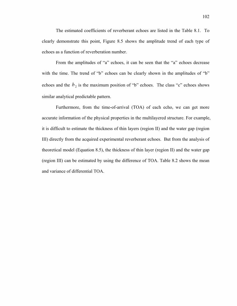
102

The estimated coefficients of reverberant echoes are listed in the Table 8.1. To

clearly demonstrate this point, Figure 8.5 shows the amplitude trend of each type of

echoes as a function of reverberation number.

From the amplitudes of “a” echoes, it can be seen that the “a” echoes decrease

with the time. The trend of “b” echoes can be clearly shown in the amplitudes of “b”

echoes and the 2b is the maximum position of “b” echoes. The class “c” echoes shows

similar analytical predictable pattern.

Furthermore, from the time-of-arrival (TOA) of each echo, we can get more

accurate information of the physical properties in the multilayered structure. For example,

it is difficult to estimate the thickness of thin layers (region II) and the water gap (region

III) directly from the acquired experimental reverberant echoes. But from the analysis of

theoretical model (Equation 8.5), the thickness of thin layer (region II) and the water gap

(region III) can be estimated by using the difference of TOA. Table 8.2 shows the mean

and variance of differential TOA.

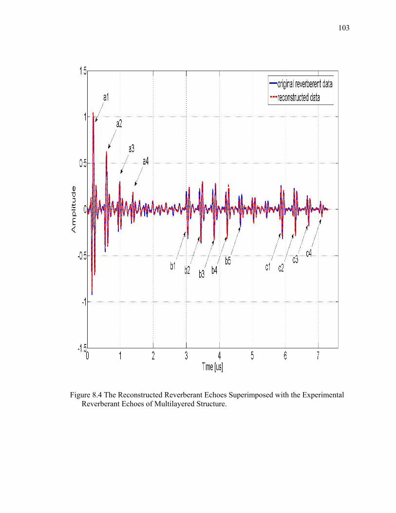
103

Figure 8.4 The Reconstructed Reverberant Echoes Superimposed with the Experimental Reverberant Echoes of Multilayered Structure.

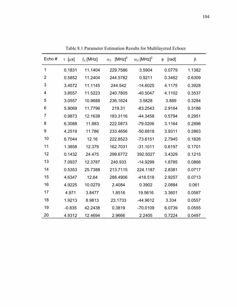
104

Table 8.1 Parameter Estimation Results for Multilayered Echoes


1 0.1831 11.1404 229.7586 3.5904 0.0779 1.1382

2 0.5852 11.2404 244.5782 0.9211 0.3462 0.6309

3 3.4572 11.1145 244.542 -14.6025 4.1175 0.3928

4 3.8557 11.5223 240.7805 -40.5047 4.1102 0.3537

5 3.0557 10.9688 236.1624 3.5828 3.889 0.3284

6 5.9069 11.7796 219.31 -83.2543 2.9164 0.3186

7 0.9873 12.1638 183.3116 -44.3458 0.5794 0.2951

8 6.3088 11.883 222.0873 -79.0206 3.1164 0.2896

9 4.2519 11.786 233.4656 -50.6818 3.9311 0.2863

10 6.7044 12.16 222.8523 -73.6151 2.7945 0.1826

11 1.3858 12.379 162.7031 -31.1011 0.6197 0.1701

12 0.1432 24.475 299.6772 392.5027 3.4329 0.1215

13 7.0937 12.3787 240.933 -14.9299 1.8785 0.0866

14 0.5353 25.7388 213.7115 224.1187 2.8381 0.0717

15 4.6347 12.64 288.4906 -418.518 2.9257 0.0713

16 4.9225 10.0279 2.4084 0.3902 2.0884 0.061

17 4.971 3.8477 1.8516 19.5616 3.3601 0.0587

18 1.9213 8.9813 23.1733 -44.9612 3.334 0.0557

19 -0.835 42.2438 0.3819 -70.0109 6.0739 0.0555

20 4.9312 12.4694 2.9666 2.2405 0.7224 0.0497

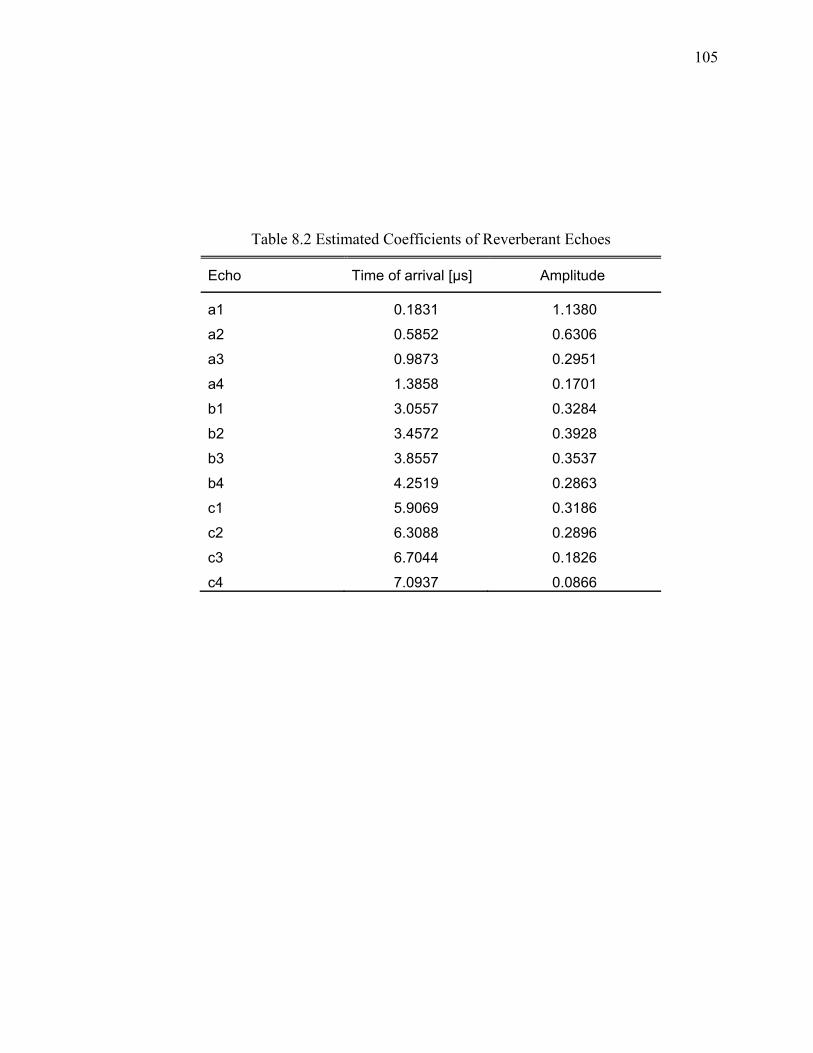
105

Table 8.2 Estimated Coefficients of Reverberant Echoes

Echo Time of arrival [μs] Amplitude

a1 0.1831 1.1380

a2 0.5852 0.6306

a3 0.9873 0.2951

a4 1.3858 0.1701

b1 3.0557 0.3284

b2 3.4572 0.3928

b3 3.8557 0.3537

b4 4.2519 0.2863

c1 5.9069 0.3186

c2 6.3088 0.2896

c3 6.7044 0.1826

c4 7.0937 0.0866

106

1 2 3 40

0.2

0.4

0.6

0.8

1

1.2

Reverberation number

Am

plitu

de

a echob echoc echo

Figure 8.5. Comparison of Envelope of Class “a” Echoes, “b” Echoes and “c” Echoes.

107

Table 8.3 Thickness Estimation of Multilayered Structure ( 31 ≤≤ k )

Difference of TOA Mean [μs] Variance

kk aa −+1 0.4009 4.3200e-6

kk bb −+1 0.3987 7.0633e-6

kk cc −+1 0.3956 1.3363e-5

kk ab −

2.8698 9.4425e-6

kk bc −

2.8483 2.0569e-5

108

8.4 Summary

In this chapter, we have analyzed theoretical model of multilayer structure. An

echo classification model of multilayered structure has been developed to reveal the

physical nature of reverberant path and re-grouped the general expression of reverberant

signal into different type of sequential echoes based on the traveling distance in the media.

The chirplet signal decomposition algorithm has been utilized to reconstruct the

experimental ultrasonic multilayered reverberant echoes with high accuracy. The

expected echo patterns, based on the theoretical model, not only have been shown in the

acquired experimental ultrasonic data, but also shown by the parameter estimation results

of chirplet signal decomposition algorithm. Through extensive experimental studies we

have shown that the reverberation model of thin layers coupled with chirplet signal

decomposition allows for a very accurate estimation of transmission/reflection properties

of each layer and also leads to an accurate estimation of the thicknesses of the layers by

an order of magnitude beyond the resolution of the ultrasonic measuring system.

109

CHAPTER 9

EMBEDDED FPGA-BASED DSP SYSTEM FOR SIGNAL DECOMPOSITION

9.1 Introduction

Field programmable gate arrays (FPGAs) are digital integrated circuits that

contain configurable logic blocks (CLBs) along with programmable interconnects

between these blocks. The Virtex series FPGAs are intended as system integration

platform which offer a combinations of performance, capability, and low system cost.

The Virtex integrates high level of system functions such as processors, delay lock loops,

clock managers, memory, and serial transceivers on a single FPGA chip [Xil06a].

Due to the flexibility of the FPGA to add custom hardware to accelerate software

bottlenecks and its quick development time, speeding the prototype process by allowing

in-platform testing and debugging of the system, we choose the Xilinx University

Program Virtex II Pro (XUPV2P) development board to verify the CTSD algorithm. The

XUPV2P board provides an advance hardware platform that has a 100 MHz system clock

and consists of a high performance Virtex-II Pro platform FPGA (i.e., XC2VP30)

surrounded by a comprehensive collection of peripheral components such as RS-232, on-

board 10/100 Ethernet device, up to 2GB of Double Data Rate(DDR) SDRAM, AC-97

audio CODEC, and on-board video port[Xil05].

Moreover, Xilinx provides its own implementation of a 32 bit RISC processor

soft core (i.e., MicroBlaze), which is tailored and optimized for implementation in Xilinx

FPGAs with minimum configurable logic resource. It features a 5-stage pipeline, with

most instructions completing in a single cycle. Both instruction and data words are 32

bits. Many aspects of the MicroBlaze can be configured at compile time due to the

110

configurable nature of FPGAs[Xil06a]. The XC2VP30 FPGA can be configured to

contain multiple MicroBlaze cores for multiprocessor system design. One of the most

useful features of the MicroBlaze is the fast simplex link (FSL) bus, which provides a

simple and high-throughput point-to-point communications between MicroBlaze and

custom hardware cores. The MicroBlaze has special assembly instructions to place and

retrieve data on and from the FSL bus.

In this chapter, the CTSD algorithm is implemented as a System-on-Chip (SoC)

based on Xilinx Virtex-II Pro FPGA to rapid prototype and further probes its suitability

for embedded hardware [Sor06]. The CTSD algorithm is implemented in software and

profiled with standard software tools to identify the parts of the algorithm which consume

the most execution time. The dedicated hardware accelerator is designed to increase the

performance of the embedded system. Simulated and experimental ultrasonic signals are

used to verify the functionality of the system design.

9.2 Embedded DSP System Based on Xilinx Virtex II Pro FPGA

From a computational complexity standpoint, the complexity of the chirplet

transform, a correlation operation between the signals and the scaled chirplet kernels (see

Equation 3.2), is )( mnO , where m is the number of scaled chirplets, and n is the

number of samples in the signal. The windowing process of chirplet transform is a linear

search with computational complexity )( nO . In other words, the time-frequency

representation of the signal depends on the sampling frequency and the scale size of the

chirplet kernel. Meanwhile, in the successive parameter estimation stage, each parameter

111

is estimated through maximization of the correlation between windowed signal and

chirplet kernel. The accuracy is dependent on the step size used to estimate the parameter.

The C implementation of the CTSD algorithm is profiled using GNU tools to

isolate which parts of the algorithm consumed the most execution time. The chirplet

transform and successive parameter estimation process occupied most of execution time.

The chirplet transform and windowing algorithm consumes on average 45.3% of the total

processing time. The successive parameter estimation consumes on average 40.3%

processing time. Further analysis shows that forward and inverse Fourier Transform

consume the majority of the windowing algorithm execution time (72.1%). Moreover, in

the successive parameter estimation stage of the algorithm, the trigonometric functions

and exponent functions are found to be heavily used in calculating the time frequency

representation and reconstructing the signal, which are major contributors to execution

time. They are most promising candidates for hardware acceleration.

An architectural overview of the developed embedded DSP system is shown in

Figure 9.1[Sor07]. From Figure 9.1, it can be seen that this system consists of an analog

sensor (ultrasonic transmitter/receiver), an A/D converter devices to sample and digitize

the ultrasonic data, and two FPGAs (i.e., an interface FPGA and an application FPGA).

The interface FPGA pre-processes the data from A/D devices and manages queuing the

data for the application FPGA. In the application FPGA, two MicroBlaze are

implemented in the FPGA fabric. One MicroBlaze is referred to as the algorithm

processor, while the other is refereed to as the communication processor.

112

The algorithm MicroBlaze is connected to the hardware cores through

unidirectional FSL buses. The FSL buses are implemented internally as FIFO queues,

along with some control logic. Since the FSLs are unidirectional, the FSL master places

data on the bus and store in the internal buffer of FSL core. The FSL slaver is in charge

of reading the data out of FSL. The transmission occurs asynchronously. This allows the

accelerators to run with a higher clock frequency than the MicroBlaze to achieve better

performance. A dedicated cache connects the algorithm MicroBlaze and the system

memory. It speeds execution on the algorithm processor since most of the data is kept in

on-chip memory. In the design of hardware accelerator cores, based on the profile

results, those time-consuming software functions are transferred to custom hardware

accelerator cores. For the Fourier transform hardware acceleration, the FFT core, a

pipelined architecture is chosen based on decimation in frequency Radix-2 butterfly units

for maximum throughput [Sek99], offered by Xilinx is capsulated with FSL interface. A

CORDIC-based core is selected for the sine, cosine acceleration, which improves

performance by calculating both sine and cosine in hardware simultaneously [Men98].

The communication MicroBlaze is mainly to provide interfacing to fetch and send

processed results from the system. It is supplemented with hardware cores to handle

RS232, video, audio and Ethernet interfacing.

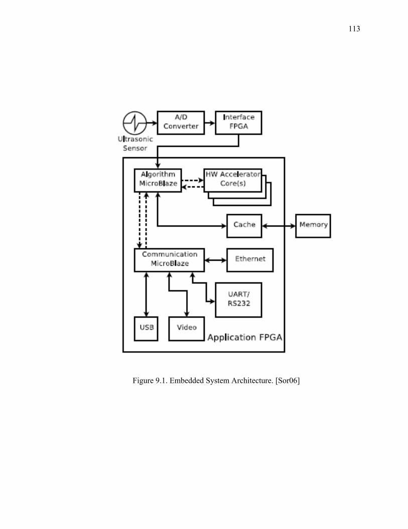
113

Figure 9.1. Embedded System Architecture. [Sor06]

114

Figure 9.2 shows the process results of processing actual experimental ultrasonic

measurements through the system. These results show that the reconstructed signal

demonstrates high fidelity to the original signal. Also, the result of estimated parameters

for each echoes from FPGA system matched the results obtained from software

implementation of the CTSD algorithm, proving the feasibility of constructing an

embedded implementation of the CTSD algorithm.

9.3 Summary

In this Chapter, A Xilinx Virtex II Pro FPGA-Based DSP system is designed to

verify the feasibility of hardware implementation of CTSD algorithm. Embedded

MicroBlaze processors and FSL buses are utilized to manage the hardware system. Based

on the profile results of CTSD algorithm, hardware acceleration cores such as FFT cores

and CORDIC-based core are used to accelerate the computation of the algorithm. The

simulation and experimental results functionally verified the system design. This work

demonstrates an embedded FPGA-based DSP system for ultrasonic detection and

estimation using the CTSD algorithm. Further algorithm analysis and hardware

acceleration strategies are expected to be done for the future real time ultrasonic signal

processing.

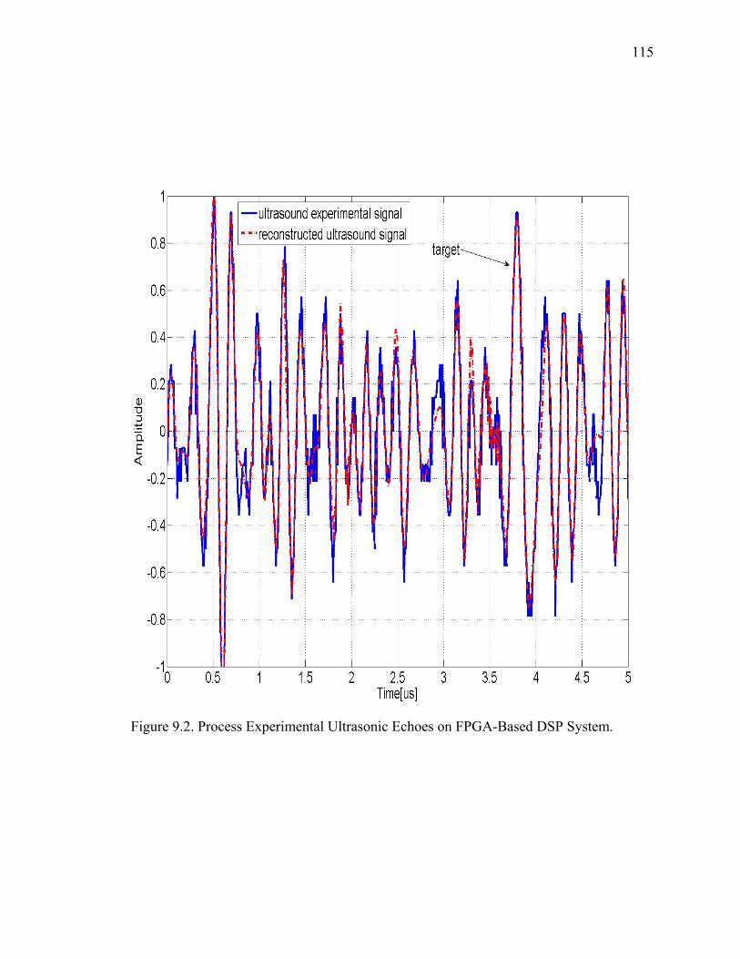
115

Figure 9.2. Process Experimental Ultrasonic Echoes on FPGA-Based DSP System.

116

CHAPTER 10

CONCLUSION AND FUTURE WORK

In ultrasonic applications, the patterns of detected echoes correspond to the shape,

size and orientation of the reflectors and the physical properties of the propagation path.

However, these echoes are often overlapped due to closely spaced reflectors and/or

microstructure scattering. Therefore, signal model and parameter estimation is critical for

these applications. In this research, we have developed chirplet signal decomposition

algorithms for signal analysis. Two different implementation strategies of decomposition

have been discussed. One is based on chirplet transform. Another one is based on the

matching pursuit framework. We developed the decomposition algorithms and

demonstrated them in different ultrasonic applications such as ultrasonic target detection,

bat chirp signal evaluation, grain size estimation, and backscattered reverberant analysis.

The chirplet signal decomposition algorithm aims to decompose the signal to be

processed into a linear combination of chirplets. In the signal decomposition algorithm

based on chirplet transform (CTSD) algorithm, from the point view of time frequency

resolution, the chirplet transform has similar resolution advantage as wavelet transform

does. The chirplet transform is used not only used as a mean for time frequency

representation, but also to estimate the echo parameters including the amplitude, time of

arrival, center frequency, bandwidth factor, phase, and chirp rate. Once these parameters

are estimated, one can achieve a quantitative representation leading to the identification

of echoes and physical property analysis of specimen. The successive parameter

estimation algorithm coupled with windowing strategy in time frequency representation

domain showed robustness in chirp signal decomposition, compared with the Gabor

117

decomposition algorithm [Car05b]. This comparison revealed one important fact about

the CTSD algorithm, that is, it uses fewer components to reconstruct the chirp type signal

and the parameters reveal the chirp nature of original signals.

Another algorithm is matching pursuit signal decomposition (MPSD) algorithm.

We incorporated statistical signal processing methods such as Maximum Likelihood

Estimation (MLE) and Maximum a Posteriori (MAP) into matching pursuit framework.

The signal analysis results show that, if proper prior information is offered, MPSD-MAP

can be more matched to the local physical properties of signals than MPSD-MLE. In both

implementations of the MPSD algorithm, the parameters of chirplet are adaptively

optimized to best match the signal residues. It avoids the exhaustive search of a large

number of dictionary function and leads to a more efficient implementation.

Furthermore, in order to determine the effect of noise level in parameter

estimation, we derived the analytical Cramer Rao Lower Bounds (CRLB) for chirplet

signal decomposition. The CRLB provides the bounds on the variance of parameter

estimators. Through Monte Carlo simulation, we demonstrated that the chirplet parameter

estimation of both algorithms is unbiased with minimum variance, i.e., it attains

analytical derived CRLB bounds. When applied to simulated ultrasonic signals, both

algorithms perform robustly, yield accurate echo estimations and result in considerable

SNR enhancements. Moreover, the MPSD algorithm outperforms the CTSD in moderate

noise levels whereas the CTSD performs better than MPSD in severe noise levels. This

can be explained by the different nature of algorithms. First, the processing domain is

different. The CTSD algorithm is to process signal and estimate the parameters in time

frequency domain whereas the MPSD algorithm performs only in time domain. Hence,

118

the noise is better suppressed in CTSD algorithm than it is in MPSD algorithm. Secondly,

the iterative optimization of MPSD algorithm may become more dependent on the initial

guess in severe noise levels.

One immediate application of the chirplet signal decomposition algorithm is

ultrasonic target detection. The CTSD algorithm has been evaluated using an ultrasonic

experimental backscattered signal consisting of many interfering echoes to detect a target

embedded in it. The reconstructed signal and time frequency representation showed that

the target echo was successfully detected and the parameters can be used to further

evaluate and analyze the physical properties.

We studied the performance of our algorithm in an experimental bat chirp echoes,

which is emitted by a large brown bat and used as the benchmark signal in literatures for

time frequency analysis. The time frequency representation shows that the bat chirp

signal is highly overlapped in both time and frequency domain, which add the difficulties

in the signal analysis. The bat chirp signal has poor SNR and contains heavily

overlapping chirp components. The chirplet signal decomposition not only successful

analyzes the contents of bat echoes as the other literatures did, but offer the details of

parameters for better scientific analysis of the species.

Another application of our algorithms is grain size estimation, which is critical to

determine the mechanical properties of materials. We reviewed a model for the ultrasonic

grain backscattered signal and discussed the effect of frequency dependent scattering and

attenuation. By estimating the expected frequency, our algorithm verified the spectral

shift trend in different specimens which were processed under different heat treatment

119

and have different grain size. Our algorithm exhibits a new angle to extract the mean

grain size information from ultrasonic backscattering echoes.

One can also use the chirp signal decomposition algorithms in the classification of

ultrasonic multilayered reverberant echoes. An echo classification model of multilayered

structure has been developed to reveal the physical nature of reverberant. Our algorithm

has been utilized to successfully classify different type of echoes in ultrasonic

experimental reverberant signal and estimate the physical parameters of multilayered

structure.

Furthermore, an embedded FPGA-based DSP system is successfully designed to

verify the feasibility of hardware implementation and acceleration for the CTSD

algorithm.

Overall, it has been shown through computer simulation and analysis of

experimental data that the chirplet decomposition algorithms can efficiently decompose

the nonstationary signal and estimate the parameters of the chirplets. The estimated

parameters have been successfully used to locate the target echo in ultrasonic

backscattered signal, evaluate grain size of material, and classify ultrasonic multilayered

reverberant echoes. This type of study addresses a broad range of applications such as

target detection, data compression, deconvlution, object classification, velocity

measurement, and material characterization.

120

BIBLIOGRAPHY

[Adl96] Adler, J., B. Rao, and K. Delgado. “Comparison of Basis Selection Methods.” Proceeding of IEEE Asilomar Conference on Signals, Systems, and Computer Frequency and Time Scale Analysis. Pacific Grove, CA (November 1996):252-257. [And87] Adnrieux, J., M. Feix, G. Mourgues, P. Bertrand, B. Izrar, and V. Nguyen.

“Optimum Smoothing of the Wigner Ville Distribution.” IEEE Transactions on Acoustics, Speech, and Signal Processing. 35.6(June 1987):764-769.

[Ant92] Antonini, M., M. Barlaud, P. Mathieu, and I. Daubechies. “Image Coding Using Wavelet Transform.” IEEE Transaction on Image Processing.1.2 (April 1992): 205-220. [Boa03] Boashash, B., Time Frequency Analysis. Massachusetts: Elsevier Science, 2003. [Bul98] Bultan, A., and O. Arikan. “ A Parallelized Matching Pursuit Algorithm for the Four Parameter Chirplet Decomposition.” IEEE International Symposium on Time Frequency and Time Scale Analysis. 1.1(October 1998):421-424. [Cap03] Capus, C., and K. Brown. “Short Time Fractional Fourier Methods for the Time Frequency Representation of Chirp Signals.” Journal of the Acoustical Society of America.113.6 (June 2003): 3253-3263. [Car05a] Cardoso, G., and J. Saniie. “Ultrasonic Data Compression via Parameter Estimation.” IEEE Transaction on Ultrasonics, Ferroelectrics and Frequency Control.52.2 (February 2005): 313-325. [Car05b] Cardoso, G., Compression, Estimation, and Analysis of Ultrasonic Signals.

Chicago: Illinois Institute of Technology May 2005.

[Cha06] Chaux, C., L. Duval, and J. Pesquet. “ Image Analysis Using a Dual Tree M Band Wavelet Tranform.” IEEE Transaction on Image Processing.15.8 (August 2006): 2397-2412.

[Che98] Chen, S., D. Donoho, and M. Saunders. “Atomic Decomposition by Basis Pursuit.” SIAM Journal on Scientific Computing.20.1 (August 1998):33-61. [Cla80] Classen, T., and W. Mechlenbrauker. “The Wigner Distribution – a Toll for Time Frequency Signal Analysis.” Philips J. Res.35 (1980): 217-250.

121

[Coh89] Cohen, L. “Time Frequency Distributions – a Review.” Proceeding of IEEE.77.7 (July 1989): 941-981. [Cot98] Cotter, S., M. Murthi, and B. Rao. “Fast Basic Selection Methods.” Proceeding of IEEE Asilomar Conference on Signals, Systems, and Computer Frequency and Time Scale Analysis. Pacific Grove, CA (November 1997):1474-1478. [Cui06] Cui, J., and W. Wong. “The Adaptive Chirplet Transform and Visual Evoked Potentials.” IEEE Transaction on Biomedical Engineering.53.7 (July 2006): 1378-1384. [Dau90] Daubechies, I. “The Wavelet Transform, Time Frequency Localization and

Signal Analysis.” IEEE Transaction on Information Theory.36.5 (September 1990):961-1005.

[Dau03] Daubechies, I., Ten Lectures on Wavelets. Philadelphia: Society for Industrial

and Applied Mathematics, June 1992. [Dem00] Demirli, R., and J. Saniie. “Model Based Time Frequency Estimation of Ultrasonic Echoes for NDE Applications.” IEEE Ultrasonics, Ferroelectrics and Frequency Control Symposium.1.1 (October 2000): 785-788. [Dem01a] Demirli, R., and J. Saniie. “Model Based Estimation of Ultrasonic Echoes. Part I: Analysis and Algorithms.” IEEE Transaction on Ultrasonics, Ferroelectrics and FrequencyControl.48.3 (May 2001): 787-802. [Dem01b] Demirli, R., and J. Saniie. “Model Based Estimation of Ultrasonic Echoes. Part II: Nondestructive Evaluation Applications.” IEEE Transaction on Ultrasonics, Ferroelectrics and FrequencyControl.48.3 (May 2001):

803-811.

[Dju90] Djuric, P., and S. Kay. “Parameter Estimation of Chirp Signals.” IEEE Transaction on Acoustics, Speech and Signal Processing.38.12 (December 1990): 2118-2126. [Don06] Donnelly, D.“The Fast Fourier Transform for Experimentalists. Part VI. Chirp of a Bat.” Computing in Science and Enigeering.8.2 (March 2006): 72-78. [Fan02] Fan, W., H. Zou, Y. Sun, Z. Li, and R. Shi. “Decomposition of Seismic Signal via Chirplet Transform.” Proceeding of IEEE 6th International Conference on Signal Processing, Beijing, China (August 2002): 1778-1782. [Fen01] Feng, A., X. Wu, and Q. Yin. “Fast Algorithm of Adaptive Chirplet Based Real Signal Decomposition.” IEEE International Symposium on Circuits and Systems.2.1 (March 2001): 6-9.

122

[Gab46] Gabor, D. “Theory of Communication.” Journal of IEE.93 (June 1946): 429-457. [Gre96] Gregorio, A., and M. Savino. “Interpolated Smoothed Pseudo Wigner Ville Distribution for Accurate Spectrum Analysis.” IEEE Transaction on Instrumentation and Measurement.45.4 (August 1996): 818-823. [Gri96] Gribonval, R., P. Depalle, X. Rodet, E. Bacry, and S. Mallat. “Sound Signals Decomposition Using a High Resolution Matching Pursuit.” Proceeding of International Computer Music Conference, Hongkong, China (August 1996): 293-296. [Gro84] Grossmann, A., and J. Morlet. “Decomposition of Hardy Functions into Square Integrable Wavelets of Constant Shape.” SIAM Journal of Mathematics Analysis.15.4 (July 1984): 723-736. [Kay98] Kay, S., Fundamentals of Statistical Signal Processing: Estimation Theory.

New Jersey: Prentice Hall, 1998. [Kri03] Krishnamachari, S., and W. Williams. “Adaptive Kernel Design in the Generalized Marginal Domain for Time Frequency Analysis.” Proceeding of IEEE International Conference on Acoustic, Speech, and Signal Processing, Adelaide, Australia (April 1994): 341-344. [Lij03] Li, J., and H. Ling. “Application of Adaptive Chirplet Representation for ISAR Feature Extraction from Targets with Rotating Parts.” IEE Proceeding on Radar, Sonar and Navigation.1.150 (August 2003): 284-291. [Lop02] Lopez, G., J. Grajal, and Q. Yeste. “Atomic Decomposition Based Radar Complex Signal Interception.” Proceeding of IEE Radar and Sonar Navigation.150.4 (August 2003): 323-331. [Lop03] Lopez, G., J. Grajal, and O. Yeste. “CFAR Detection of Chirplets in Coloured Gaussian Noise.” Proceeding of IEEE International Conference on Acoustic, Speech, and Signal Processing, Hong Kong, China (April 2003): 741-744. [Lu03] Lu, Y. “Ultrasonic NDT and Imaging System.” Research Report of Special Problem, Chicago, IL(February 2003): 1- 41. [Lu05] Lu, Y., G. Cardoso, R. Demirli, and J. Saniie. “Chirplet Transform for Ultrasonic Signal Analysis and NDE Applications.” IEEE Ultrasonics, Ferroelectrics and Frequency Control Symposium.1.1 (September 2005):

536-539. [Lu06a] Lu, Y., R. Demirli, G. Cardoso, and J. Saniie. “A Successive Parameter Estimation Algorithm for Chirplet Signal Decomposition.” IEEE

123

Transaction on Ultrasonics, Ferroelectrics and Frequency Control.53.11 (November 2006): 2121-2131. [Lu06b] Lu, Y., R. Demirli, and J. Saniie. “A Comparative Study of Echo Estimation Techniques for Ultrasonic NDE Applications.” IEEE Ultrasonics, Ferroelectrics and Frequency Control Symposium.1.1 (October 2006). [Lu07] Lu, Y., R. Demirli, E. Oruklu, and J. Saniie. “Estimation and Classification of Ultrasonic Echoes Backscattered from Reverberant Multilayered Materials.” International Congress on Ultrasound. (April 2007). [Mal89] Mallat, S. “A Theory for Multiresolution Signal Decomposition: the Wavelet Representation.” IEEE Transactions on Pattern Analysis and Machine Intelligence.11.7(July 1989): 674-693. [Mal91] Mallat, S. “Zero-Crossings of a Wavelet Transform.” IEEE Transaction on Information Theory.37.4 (July 1991):1019-1033. [Mal93] Mallat, S., and Z. Zhang. “Matching Pursuits with Time Frequency Dictionaries.” IEEE Transactions on Signal Processing. 41.12(December 1993):3397-3415. [Mal99] Mallat, S, A Wavelet Tour of Signal Processing. California: Academic Press, 1999. [Ma98] Ma, N., and D. Vray. “Bottom Backscattering Coefficient Estimation from Wideband Chirp Sonar Echoes by Chirp Adapted Time Frequency Representation.” Proceeding of IEEE International Conference on Acoustic, Speech, and Signal Processing, Seattle, WA (May 1998): 12-15. [Man92] Mann, S., and S. Haykin. “Time Frequency Perspectives: the Chirplet Transform.” Proceeding of IEEE International Conference on Acoustic, Speech, and Signal Processing, San Francisco, CA (March 1992): 417-420. [Man95] Mann, S., and S. Haykin. “The Chirplet Transform: Physical Considerations.” IEEE Transaction on Signal Processing.43.11 (November 1995): 2745-2761. [Men98] Mencer, O., M. Morf, and J. Delosme. “Application of Reconfigurable CORDIC Architectures.” Proceeding of IEEE Asilomar Conference on Signals, Systems, and Computer, Monterey , CA (June 1998):182-186. [Mey93] Meyer, Y., and R. Ryan. Waveletes: Algorithms and Applications. Massachusetts: Society for Industrial and Applied Mathematic, May 1993. [Nei99] Neill, J., and J. Williams. “A Function of Time, Frequency, Lag and Doppler.” IEEE Transaction on Signal Processing.47.3 (March 1999):

124

789-799. [Oeh97] Oehlmann, H., and D. Bric. “The Reduced Interference Local Wigner Ville

Distribution.” Proceeding of IEEE International Conference on Acoustics, Speech and Signal Processing, Munich, Germany (April 1997): 3645-3648.

[Qia92] Qian, S., D. Chen, and K. Chen. “Signal Approximation Via Data Adaptive

Normalized Gaussian Functions and Its Applications for Speech Processing.” IEEE International Conference on Acoustics, Speech, and Signal Processing, San Francisco, CA (Augest1992):141-144.

[Qia94] Qian, S., and D. Chen. “Signal Representation Using Adaptive Normalized Gaussian Functions.” IEE Transaction on Signal Processing.36.1 (March 1994):1-11. [Qia98] Qian, S., D. Chen, and Q. Yin. “Adaptive Chirplet Based Signal Approximation.” Proceeding of IEEE International Conference on Acoustic, Speech, and Signal Processing, Seattle, WA (May 1998): 1781-1784. [Rab93] Rabiner, L., Fundamentals of Speech Recognition. New Jersey: Prentice Hall, April 1993. [Rod98] Rodenas, J., and R. Garello. “Internal Wave Detection and Location in SAR

Images Using Wavelet Transform.” IEEE Transaction on Geosciences and Remote Sensing.36.5 (September 1998): 1494-1507.

[San81] Saniie, J. Ultrasonic Signal Processing: System Identification and Parameter Estimation of Reverberant and Inhomogeneous Targets. West Lafayette: Purdue University August 1981. [San82] Saniie, J., E. Furgason, and V. Newhouse. “Ultrasonic Imaging Through Highly Reverberant Thin Layers - Theoretical Considerations.” Material Evaluation.40 (January 1982):115-121.

[San89] Saniie, J. and D. Nagle. “Pattern Recognition in the Ultrasonic Imaging of Reverberant Multilayered Structures.” IEEE Transaction on Ultrasonics, Ferroelectrics, and Frequency Control.36.1 (January 1989): 80-92. [San94] Saniie, J. and M. Mohamed. “Ultrasonic Flaw Detection Based on Mathematical Morphology.” IEEE Transaction on Ultrasonics, Ferroelectrics, and Frequency Control.41.1 (January 1994): 150-160. [Sek99] Sekhar, B., and K. Prabhu. “Radix-2 Decimation In Frequency Algorithm for the Computation of the Real Valued FFT.” IEEE Transaction on Signal Processing.47.1 (April 1999): 1181-1184.

125

[Sor06] Sorenson, L., Y. Lu, F. M. Vallina, and J. Saniie. “Chirplet Transform Signal Decomposition for Echo Detection and Estimation.” Proceeding of IEEE Asilomar Conference on Signals, Systems, and Computer, Pacific Grove , CA (October 2006). [Unl96] Unluturk, M., and J. Saniie. “ Neural Networks for Ultrasonic Grain Size Discrimination” Proceeding of IEEE on Ultrasonic, Ferroelectrics, and Frequency Control.1.1 (November 1996): 669-672. [Vil48] Ville, J. “Theorie et Applications de la Notion de Signal Analytique.”

Cable et Transmission .2A (June 1948): 61-74.

[Wan91] Wang, T., J. Saniie, and X. Jin. “Analysis of Low Order Autogressive Models for Ultrasonic Grain Signal Characterization.” IEEE Transaction on Ultrasonics,Ferroelectrics, and Frequency Control.38.2 (March 1991): 116-124.

[Wan00a] Wang, G., and X. Xia. “An Adaptive Filtering Approach to Chirp Estimation and ISAR Imaging of Maneuvering Targets.” Proceeding of IEEE International Radar Conference. Alexandria, VA (May 2000): 481-486. [Wan00b] Wang, G., and X Xia. “Iterative Algorithm for Direction of Arrival Estimation with Wideband Chirp Signals.” Proceeding of IEE on Radar and Sonar Navigation.147.5(October 2000): 233-238. [Wan01] Wang, J., X. Yan, A. Costa, and D. Kasilingam. “A Weighted Decomposition of the Wigner Distribution.” Proceeding of IEEE on Signal Processing.10.11 (August 2001): 337-340. [Wan02] Wang, G., and X. Xia. “Moving Target Detection in Over the Horizon Radar Using Adaptive Chirplet Transform.” Proceeding of IEEE International Conference on Radar. Long Beach, CA (April 2002): 77-84. [Wan03] Wang, G., X. Xia, B. Root, V. Chen, Y. Zhang, and M. Amin.

“ Manoeuvring Target Detection in Over the Horizon Radar Using Adaptive Clutter Rejection and Adaptive Chirplet Transform.” Proceeding of IEE on Radar and Sonar Navigation.150.4 (August 2003): 292-298.

[Wig32] Wigner, E. “On the Quantum Correction for Thermodynamic Equilibrium.”

Physical Review (June 1932): 749-759. [Xia00] Xia, X., “Discrete Chirp Fourier Transform and Its Application to Chirp Rate Estimation.” IEEE Transaction on Signal Processing.48.11 (November 2000): 3122-3133. [Xil06a] Xilinx Inc., Xilinx Microprocessor Controller and Peripheral: MicroBlaze

126

Soft Processor Core. Xilinx, 2006 [Xil06b] Xilinx Inc., Fast Simplex Link (FSL) Bus (v2.00a). Xilinx, 2006

[Yin02] Yin, Q., S. Qian, and A. Feng. “A Fast Refinement for Adaptive Gaussian Chirplet Decomposition.” IEEE Transaction on Signal Processing.50.6 (June 2002):1298-1306.

[Zan03] Zhang, L., Y. Peng, and J. Xu. “A Chirp Signal Parameter Estimation Algorithm and its Application to SAR.” Proceeding of IEEE Conference on Radar.Huntsville, Alabama (May 2003): 228-231. [Zen01] Zeng, Z., and I. Cumming. “SAR Image Data Compression Using a Tree

Structured Wavelet Transform.” IEEE Transaction on Geosciences and Remote Sensing.39.3 (March 2001): 546-552.

CHIRPLET SIGANL DECOMPOSITION OF ULTRASONIC SIGNAL...

Documents

Transcript of CHIRPLET SIGANL DECOMPOSITION OF ULTRASONIC SIGNAL...