1

Chinese Economic Development and Input-Output Extension1

CHEN Xikang, GUO Ju-e and YANG Cuihong

ABSTRACT

There are three parts in this paper. In the first part we summarily introduce the application of

input-output analysis in China, including construction of national and regional input-output tables,

input-output tables for special sectors and enterprise input-output table, and their application in

China. Particularly, on the basis of input-output model in 1990 the National Bureau of Statistics

made a suggestion to the State Council of China for increasing additional 40 billion RMB yuan of

the investment in capital construction, the proposal was accepted by the Chinese government.

In the second part we discuss extended input-output model with assets. The main

characteristic of the model is that it allows us to examine all holding assets used in production,

not only machinery and buildings but also the labor force (or human capital), land, etc., and their

requirements are specified for each sector. Thus extended input-output model with assets

provides a better alternative to capital stock matrices in the standard Systems of National

Accounts (SNA). In this paper we will comprehensively introduce its methods and applications.

We specify term of holding and using of assets, extended input-output table with assets and its

main characteristics, method of calculation of total input coefficient with input of fixed assets,

total holding coefficient of assets, dynamic extended input-output model, etc.

In the final part we introduce the application of extended input-output model with assets in

China. Particularly, the model was successfully applied in yearly grain output prediction of China

1980-2004. Since 1980 this approach has been used in China. Every year at the beginning of May

we send annual report of yearly national grain output prediction to the governmental agencies and

1Chen Xikang, Yang Cuihong, Academy of Mathematics and Systems Science, Chinese Academy of Sciences, 55 Zhongguancun Dong Lu, Beijing, 100080, P. R. of China. Guo Ju-e, Management School of Xi’an Jiaotong University, 28 Xian Ning West Road, Xi’an, China, 710049, P. R. of China. E-mail: xkchen@mail.iss.ac.cn, guojue@mail.xjtu.edu.cn, chyang@mail.iss.ac.cn. The research was funded by the National Natural Science Foundation of China (Project No. 70131002, 60474063) and the Chinese Academy of Sciences. The authors would like to express their sincere thanks to Professors Christian DeBresson, Erik Dietzenbacher, Karen R. Polenske for their valuable comments and important suggestions.

1

2

top leaders of China. From 1980 to 2003 the main results are as follows:

First, predicted bumper, average and poor harvests are correct every year;

Second, the lead-time of prediction is more than half a year. Since 70% of China grain is

reaped in fall and harvest is ended in November, such prior forecasting report at the end of April

helps responsible governmental agencies with enough time to arrange grain consumption, storage,

imports and exports.

Third, forecasting is accurate (under 3% error) for 19 years out of 23. Error rates for 8 years

are lower than 1%, for 6 years are between 1-2%, for 5 years are between 2-3%, for 2 years are

between 3-5%, and for 2 years are between 5-8%. Overall, average error rate over 23 years is

only 1.9% compared to statistical reports from sample surveys.

Therefore, this forecasting has supported some important policy decisions. The top leaders of

China, relevant departments of Chinese government, such as State Grain Administration,

Ministry of Agriculture, Research Department of State Council, National Development and

Reform Commission, and others paid much attention and gave excellent evaluation to the

prediction.

Keywords: Chinese economic development; extended IO table with assets; total input coefficient

with input of fixed assets; direct and total holding coefficient of asset; yearly grain output

prediction

1. Constructing and Using Input-Output Tables in China

In China study on input-output analysis began in 1960. There were two research groups studying

on input-output analysis: one was in the Department of Operations Research, Institute of

Mathematics, Chinese Academy of Sciences. The other was in the Institute of Economics,

Chinese Academy of Social Sciences. During the period of “Cultural Revolution” (1966-1976) all

scientific methods of management, including input-output techniques, methods of operations

research, econometrics and others were criticized as capitalist and revisionist rubbish. It was hard

time for us. In 1972 we made a suggestion to the National Planning Commission (NPC) for

2

3

constructing a national input-output table to improve the planning work of China. The proposal

was accepted by the NPC. In 1974 under the support of NPC, National Bureau of Statistics and

National Bureau of Information, Chen Xikang and others, constructed the first experimental

input-output table of the national economy of China for 1973. Since reform and opening to the

outside world (1978-present) great changes have taken place in China. Input-output analysis has

been applied not only in macroeconomic analysis, but also in microeconomic management.

With the rapid spread of input-output technique in China, it is necessary to exchange

experience and search together for solutions to the problems in theory and applications. In 1987

the China Input-Output Society was founded. Up to the present there were 6 conferences. The

first conference was convened in 1988 in Nanchang, Jiangxi Province. The second one was in

1991 in Baotou, Inner Mongolia. The third one was in 1994 in Yinchuan, Ningxia Province. The

fourth one was in 1997 in Changchun, Jilin Province. The fifth one was convened in 2001 in

Xining, Qinghai Province. The sixth conference was convened in October, 2004 in Kunming,

Yunan Province. The number of participants of each conference was 80-130. Under the assistance

of National Bureau of Statistics (NBS) proceedings for the first 5 conferences have been

published.

Besides, the China Input-Output Society spent nearly one and a half year collecting over

one hundred papers on input-output application in China from the beginning of 2003. After

several rounds of strict examination, finally 35 papers were selected in the book entitled “Selected

Papers on Analytical Purposes of I-O Techniques in China”, edited by Xu Xianchun and Liu

Qiyun, This book was published in May 2004.

1.1. Constructing National Input-Output Table

The national input-output tables constructed to date are listed in Table 1 (Chen 1989, Karen

and Chen, 1991).

The 1973 input-output table is in physical units, while 1979, 1981, 1983 and 1992 tables

are available in both physical and value units. The physical input-output table plays very

3

4

important role in China. It is because before 1978 the most targets of the annual plan and

five-year plan, such as iron, steel, coal, oil, electricity, grain, cotton, etc., were given in physical

units. After 1978 in order to measure the amounts of generation of pollution, pollution abatement

and natural resource use, physical input-output table and value-physical table is also very useful.

Before 1987 all value input-output tables are in Material Balance System (MBS). It means only

material production is included in the first quadrant (intersectorial flow part) of input-output table.

Since 1987 all input-output tables are constructed according to the System of National Accounts

(SNA) of United Nations.

In 1987 the State Council of the People’s Republic of China decided that every 5 years

(1987, 1992, 1997, 2002 and so on) China would do special input-output survey to construct

national and regional input-output tables. Since 1987 the NBS constructs input-output table

regularly.

1.2. Constructing Regional and Interregional Input-Output Tables

Between 1979 and 1986, 25 of China’s 29 provinces, autonomous regions, and municipalities

constructed regional input-output tables (Liu and Wu, 1991). Shanxi is the first region to compile

regional input-output tables for 1979. Heilongjiang and Shanghai constructed their tables for

1981. Tianjin and Henan constructed their tables for 1982. Liaoning, Guizhou, Gansu and Hunan

compiled the tables for 1983. Hebei, Jilin, Zheijing, Sichuan, Fujian and Xinjiang Uygur

Autonomous region compiled their tables for 1984. Beijing, Jiangsu, Anhui, Jiangxi, Hubei,

Guangdong, Guangxi Zhuang Autonomous region, Shaanxi, Qinghai, and Ningxia Hui

Autonomous region constructed their tables for 1985. Beside provincial tables, many cities and

counties, for example, Wuhan, Dalian, Xi’an, Chongqing and Harbin constructed their regional

tables. The techniques to construct regional tables are flexible and varied. For example, the staff

of Shanxi, Heilongjiang, Liaoning provinces and Wuhan city constructed their tables, using

“Direct Decomposition Method” on the basis of special surveys, in which all large and

median-sized enterprises and part of small enterprises were included. The staff of Tianjin city and

4

5

Guangdong province constructed the tables by “UV Technique” recommended by the Statistics

Bureau of United Nations.

In 1987, 1992 and 1997 the NBS of China constructed national input-output tables under

general and special surveys. All provinces, autonomous regions, and municipalities except Tibet

and Hainan constructed their regional input-output tables. The sector classification and the scale

of regional tables are the same as national input-output tables.

Besides regional input-output tables, some institutions and scholars also did some work in

constructing interregional input-output table. For example, Information Center of Jiangsu

Province, etc. constructed Jiangsu interregional table for 1985, in which national economy of

Jiangsu is divided into two parts: South and North. The southern part has a developed economy

and northern part has a less developed economy. The table is used to analyze the effect of an

additional investment in the North on Jiangsu economy. Development Research Center under

State Council of China constructed interregional table of China with 3 regions and 10 sectors for

1987 and other years. State Information Center of China constructed interregional table with 8

economic zones: North-East Zone (Liaoning, Jilin and Heilongjiang), Beijing-Tianjin Zone

(Beijing and Tianjin), Northern Coastal Zone (Hebei and Shandong), Central Coastal Zone

(Jiangsu, Shanghai and Zhejiang), Southern Coastal Zone (Fujian, Guangdong and Hainan),

Central Zone (Shanxi, Henan, Anhui, Hubei, Hunan and Jiangxi), North-West Zone (Inner

Mongolia, Shaanxi, Ningxia, Gansu, Qinghai and Xinjiang) and South-West Zone (Sichuan,

Chongqing, Guangxi, Yunnan, Guizhou and Tibet) for 1997. The table was constructed on the

basis of 1997 regional input-output tables and used gravity model to determine the interregional

coefficient under the transportation statistical data (Zhang and Zhao, 2004). Under the

organization of the Institute of Developing Economies of Japan the State Information Center,

together with USA and other 8 Asian countries and regions, compiled the linked international I-O

tables for 1985, 1990 and 1995, they are constructing the table for 2000.

1.3. Constructing Input-Output Tables for Special Sectors

5

6

In addition to general tables for all sectors we have compiled input-output tables for special

sectors, such as input-output tables of agricultural sectors for 1982, 1984, 1987, 1992 and 1997,

table of mechanical and electronic industry for 1983, table of chemical industry for 1979 and

1985, table of urban water-economy in Beijing for 1982, table of colour television for 1985, table

of weapons industry, table of copper industry, table of information industry, table of

environment-economy for Tianjin city, Liaoning province and China, table of taxes for 1987,

table of energy consumption and greenhouse gas emission for 1992, table of information for

China (1987) and for Yueyang county, Hunan Province, table of foreign trade for 1995, table of

township and village enterprise for Shanxi Province and China for 1992, 1995, and 1997, table of

air pollution input-output table for Beijing, etc.

The 1982 and 1984 input-output table for agricultural sectors was constructed by staff of

Institute of systems Science, Chinese Academy of Sciences and others under the support of Rural

Development Research Centre of the State Council of China. The tables were classified into a

physical table; two value tables (at current prices and 1980 constant price) and an energy table.

There are 40 agricultural products in the first part of physical table, 24 agricultural sectors in

value table, and 47 agricultural sectors in energy table. In order to construct these tables a special

survey was conducted in 120 counties to collect the data not provided by the existing accounting

system of China. The energy table is very interesting and was used to calculate the output-input

ratio of artificial energy and study the ecological balance in agriculture (Karen and Chen, 1991).

1.4. Constructing Enterprise Input-Output Table

One of the important characteristics of the application of input-output techniques in China is to

use the techniques in enterprise planning and cost calculation, and to construct enterprise

input-output table.

In 1964 Chen Xikang and Li Bingquan constructed the first enterprise input-output table for

Tianjin Chemical Factory. It was a physical table, which includes 25 self-made products and

service sectors in the first part and 30 purchased material and energy products in the third part of

6

7

the table.

In 1965 Li Bingquan and others of the Institute of mathematics, Chinese Academy of

Sciences, went to Anshan Iron and Steel Corporation, the biggest iron and Steel Corporation in

China, and constructed a physical enterprise input-output table. The table included 55 self-made

products, 10 retrieved metallic materials and 8 purchased metallic products. The table served the

needs of the analysis of the metal equilibrium and the management of the corporation. For

example, the table created a planned internal price system within the corporation and constructed

a long-term development program of the corporation (Li, 1991, 2004).

So far, more than 100 large and medium-sized enterprises of China have constructed

input-output tables, for example, Huabei Pharmaceutical Factory, Hangzhou Iron and steel Plant,

Shanghai Gaoqiao Chemical Plant, Synthesis Plant under Jilin Chemical Industry Corporation,

Qingdao Second Rubber Plant, Tianjin Bicycle Factory, Yanshan Petrochemical General

Corporation, Yunan Chemical Plant and so on.

Tong Rencheng and Wang Dong constructed input-output table for Hualin Robber

Corporation, one of the large sized robber corporation of China, and made a system of cost

calculation and prediction (Tong and Wang, 1992). The input-output table included about 400

products and service. The system is useful to calculate cost of products and to predict profits and

gross value output. Since 1991 the manager of the corporation used the system in operational

management. Besides, Tong Rencheng and others used input-output method in oil piping

enterprise of Liaoning Province (Tong, 2004).

1.5. Some Applications

Chinese economists find that input-output techniques are very useful for economic analysis,

planning, management and forecasting. In China input-output analysis is popular for economists,

for example, Input-Output Techniques, written by Chen Xikang and Li Bingquan，Beijing

International Broadcast Press, 1983, had 223 thousand copies. Because of his contribution to

input-output technique, Wassily Leontief was the most famous foreign economist of China in the

7

8

eighties and nineties of the 20th century.

(1) Using input-output techniques to check the equilibrium of the annual plan and the

five-year plan. For example, in 1978, 1979 and 1981 we used revised input coefficients of 1973

physical input-output table to check the material balance of the 1979, 1980 and 1991 national

economic plan of China (Chen and Xue, 1984). We found that there was serious unbalance in

some energy products, particularly electricity, crude oil and coal, and about 15 million tonnes of

crude oil in 1975 was burned directly in electricity sector and others instead of coal and fuel oil.

We made suggestion to the National Planning Commission for stop burning of crude oil and to

increase amount of crude oil export.

(2) Making suggestion on Chinese economic development. At the beginning of 1990 the

National Bureau of Statistics used 1987 national input-output table to check the main targets of

the annual plan of 1990 and found that total investment of capital construction by government

was too small. It made a negative impact on the economic growth of China. Then the National

Bureau of Statistics made a suggestion for increasing additional 40 billion RMB yuan of the

investment of the capital construction to the State Council of China. The State Council accepted

the suggestion. Former Premier Li Peng gave a very nice appraisal on it and the suggestion played

an important role in Chinese national economic development of 1990 (Li, Q., 1992).

(3) Using input-output techniques in price reform and studying effect of change in price of

some products. The Price Research Centre of the State Council and the Price Research Institute of

the National Price Bureau organized the calculation of theoretical prices in 1981, 1983 and 1985.

In 1981 it included 1200 categories of products, in which 100 agricultural, 40 mineral, 600

manufactured, 100 light industrial, and 100 textile products (Li, M., 1988). In 1990 and 1991 the

Ministry of Finance used input-output model to calculate the effect of raising price in some

important products, for example grain, coal, etc. and increasing taxes on government budget and

price level. Some people of the Ministry of Railway and others used input-output methods to

study the effects of raising price in railway transportation on the national economy. In 1999 the

Academy of Mathematics and Systems Science used input-output model to calculate the effect of

8

9

change in crude oil price of world market on the GDP and the price level of China.

(4) Studying the effect of China’s entry to the WTO on the economic development of China.

Professor Li Shantong and her colleagues in the Development Research Center under the State

Council used I-O techniques and CGE model to study the effect of China’s entry to the WTO on

the GDP of China and Guangdong Province. The direct and indirect effect on the growth rate of

GDP in the period from 2001 to 2010 is more than 0.5% (Li, Zhai and Liu, 2001)

(5) Studying the effect of Olympic game in 2008 on the economic development of China.

Beijing has won the bid for 2008 Olympic Games. The Olympic Game has deep influences on the

policy, economy, culture and other aspects of China. Liao Mingqiu, Wei Xiaozhen and others in

Beijing Bureau of Statistics and universities, construct China Beijing Olympic Economic Model,

using input-output analysis, econometrics and optimization to study the effects.

(6) Using input-output techniques in foreign trade. Chen Xikang, with the collaboration of

Lawrence J. Lau, Professor of Department of Economics, Stanford University and others,

compiled China’s 1995 foreign trade input-output table and studied the effect of Chinese exports

on the GDP, employment and gross output. They find that China increases exports to the world

market by 1 USD, China’s GDP will increase 0.57 USD. China increases exports to United States

by 1 USD, China’s GDP will increase 0.49 USD (Chen, 2001). Shen Lisheng and Wu Zhenyu

studied the effect of imports by method of distribution coefficient on the Chinese economy and

reasonability of the structure of foreign trade products (Shen and Wu, 2004)

(7) Using input-output model in environment protection. For example, Tianjin Environment

Protection Bureau and Tianjin Statistical Bureau constructed environment

protection-economy-input-output tables for 1982, 1985 and 1992. From the tables they found that

there was good relationship between economic structure and pollution abatement. Tianjin

Environment Protection Bureau used 1987 tables to predict the discharge amount of 4 pollutants

(heavy metal, COD, dust and waste residue) of Tianjin City in 1995.

2 Extended Input-Output Model with Assets

9

10

In the process of using input-output analysis, in the 1980s we began to study extended

input-output model with assets. The main idea of the model is that assets, including fixed assets,

inventory, labor, financial assets, and natural resources, play a very important role in production.

The common input-output table does not include assets. Assets have to be incorporated into the

input-output table and a set of corresponding model has to be established. Since 1980, Chinese

input-output researchers have used the extended input-output model in grain output prediction,

water conservancy, economic-environmental analysis of township and village enterprises, foreign

trade, finance, and other areas.

Many scholars have done work on assets issues. In particular, Leontief proposed a dynamic

input-output model using a capital coefficient matrix. He and several researchers at the Harvard

Economic Research Project not only studied dynamic models theoretically, but also led empirical

work on the construction of matrices of capital coefficients, including fixed capital stocks and

inventories by sector (Leontief, Chenery, Clark, Duesenberry, Ferguson, Grosse, A. P., Grosse, R.

N., Holzman, Isard, & Kistin, 1953). Following Leontief, many scholars—for example, Ghosh

(1964), Alman (1970), Carter (1970), Green (1971), Grossling (1975), Peterson & Schott

(1979)—studied issues concerning capital coefficients and labor. In Japan there has been much

meaningful research on capital measurement, including an estimation of capital formation matrix

every five years since 1970 and an estimation of capital stock matrix in 1955, 1975, and other

years (Kuroda & Nomura, 2003). Concerning natural resources, Leontief and his colleagues

calculated the production and consumption of six metallic and three energy resources for 2000

and divided developing countries into two groups: developing with major mineral resource

endowment and other developing countries (Leontief et al, 1977). The following work is seen as

an extension of this research agenda. The common input-output table, however, has up to now not

regularly included assets, held or used. In this paper we will introduce an extended input-output

model with assets and apply it to prediction of grain output in China.

2.1. Holding and Using of Assets

10

11

In 1984, when we constructed input-output table for agriculture to study grain issues in China, we

had to face the fact that both cultivated land and capital play a critical role in agricultural

production, but the common input-output model did not include land, labor, or any forms of

capital assets used in agricultural production. It was therefore necessary for us to extend the

normal input-output models to include fixed assets, inventory, labor, land, water, and other assets.

Holding and using assets in production is a prerequisite for production. No production

process can proceed without the presence of required quantities of assets, including capital,

skilled or unskilled labor, and natural resources. Production scale and economic benefits also

depend on the quantity and quality of the available assets. Natural resources play a critical role in

some sectors, such as mining and agriculture.

In normal input-output models, the term “input” represents the consumption of various

production factors in the process of economic activities. It may be seen from the meaning of

“total input” in the input-output table. The total input is equal to the sum of intermediate inputs

and primary input, which are consumptions of various materials, energy, services and primary

factors.

With assets we refer to holding and using various assets and elements that are used by each

sector at a point in time. Assets consist not only of fixed assets (such as machinery and

construction), but also of inventories, financial assets, labor force (educated or not, skilled or not),

natural resources, intangible assets, and others.

There exists close inter-relationships between factor inputs, assets held and used, and output.

First, assets are a prerequisite for input and output. Without assets there will be neither input nor

output. The quantity and quality of output are directly dependent on the quantity and quality of

assets held and used. In particular, modern production requires higher-quality assets.

Second, assets are related with output and input. For example, some parts of output are used

as fixed capital formation and thus as an increase in stocks in order to improve the quality and

quantity of fixed assets. For example, in order to have a more skilled and highly skilled labor

force, it is necessary to have more output in the education sector.

11

12

Finally, input is dependent on assets used. For example, because modern agriculture uses

advanced agricultural machinery and highly skilled managers and workers as assets, its input

coefficients, such as oil, electricity, chemical fertilizer, and chemical pesticides, are different from

the input coefficients of traditional agriculture.

The input-output model reflects the interdependence between factor inputs (consumption) and

outputs in production, but the normal input-output model does not include an asset section; nor

does it reflect the inter-relationships between assets and outputs. Because there is no asset section,

especially fixed assets and financial assets (other than machinery and construction in the capital

stock matrix), the current input-output tables may lead to a misconception that by using the

following equations the vector of total output of all sectors can be determined given a final

demand vector.

fAIx 1)( −−= (1)

Where:

x denotes gross output vector

f denotes final demand vector and contains the row sums of the final demand matrix F

I and A represent identity matrix and direct input coefficient matrix, respectively

In fact, even if f has been determined, x cannot be obtained if certain quantities of the assets held

and used, such as fixed assets, natural resources, and labor, are not assured (Chen, 1990).

The common input-output model shows inter-relationships between input and output; the

extended input-output model with assets shows not only relationships between factor input and

output, but also relationships between assets and output, and linkages between assets and factor

input.

From the point of view of the system of national accounts and statistics, factor input and

assets held and used are different types of statistical indicators. Factor input is listed in the

category of flows, and assets belong to category of stocks. In common input-output tables, all

entries, including intermediate and primary input, intermediate final demand, and output belong

to flows. All assets held—for example, natural resources, labor, fixed assets, inventory, and

12

13

financial assets—are stocks. As Hicks wrote, current activity of production and consumption are

called “flow activity”, while the holding of assets is called “stock activity” (Hicks, 1965).

Flows reflect creation, transformation, transaction, or exchange in economic activities within

a period of time. Their quantity depends directly on the length of the process. Steel output per

year, for instance, is equal to roughly 12 times the output per month. However, stocks are in

position or in “holding” at a point in time. The quantity has no direct relation with length of the

production period. For example, the number of workers in the steel sector at the beginning of year

is roughly equal to that at the end of the year. Generally, stocks are preconditions of flows and the

intensity and quantity of flows are determined by the status of stocks. Increases in stocks and

reproduction of stocks are dependent on the flows. There is close and reciprocal relationship

between the two.

In summary, the common input-output model shows relationships only between flows; the

extended input-output model with assets shows not only linkages between flows, but also

between stocks and flows and between stocks themselves.

2.2. Extended Input-Output Model with Assets and Its Main Characteristics2

The extended input-output table is shown in Table 2. In order to compile this table it is necessary

to have a large quantity of data. Because data in most applications in China are scarce, we more

often use some simplified forms of the table. Table 3 is one of the simplified forms.

[TABLES 2 AND 3 ABOUT HERE]

These tables differ from a normal input-output table in two ways. First, the normal

input-output table includes only factor input in the vertical direction, whereas the extended

2 In some previous books and many papers published in China and a few abroad, the

model was called input-“occupancy”-output model. The meaning of the term

“occupancy” was meant to stand for, in English, “holding and using assets” at a point of

time by a sector, where assets include fixed assets, inventory, financial assets, labor,

natural resources, and so on.

13

14

input-output table with assets includes two sections vertically: factor input section and holding of

assets section (Chen, 1990, 1998). The asset matrix may be very large and consists of

following parts:

OW

1). Fixed assets. From the table we find not only the total amount of fixed assets, but their

specified use by every production sector and the physical contents of the fixed assets (e.g.,

construction, machinery, transport vehicles, etc.) distributed according to their sector of origin.

Therefore, we have a square matrix of fixed assets with n orders (some rows of the matrix consist

only of zeros);

2). Inventory. This is also a square matrix with n orders that gives the inventories originating

from sector I that are held by sector j;

3). Financial assets. An matrix with financial assets held by sector j for each of the

categories (such as currencies; deposits; loans; shares; securities other than shares; advances

and trade credits; and other financial assets);

nnf ×

fn

4). An matrix with labor used by sector j for each of the schooling categories

(such as illiterate; primary school; junior secondary school; senior secondary school; college; and

higher level, or according to unskilled, skilled, and highly skilled levels). Labor is usually

expressed in physical units.

nnl × ln

5). Natural resources: land, water, subsoil assets, and so on. Natural resources are also

expressed in physical units;

6). An matrix with intangible assets held by sector j for each of the categories

(such as patents; trade marks; and other intangible assets).

nn i × in

In the current system of national accounts (SNA) there are capital accounts, financial

accounts, and so on. Usually, the total amounts of fixed assets, inventory, financial assets, labor,

and natural resources are shown in the related accounts of SNA, but in the current SNA there are

no detailed capital data in input-output form by sector of use and origin. In the normal

input-output table, fixed capital formation and changes in inventories are column vectors; they are

14

15

total amounts for all sectors of the economy. We cannot find the figures for fixed capital

formation or changes in inventories for every sector of use. This means that the current SNA and

the normal input-output table cannot reflect the relationships between output and asset held and

used by each sector.

The advantage of the extended input-output model over the SNA model is that it specifies the

quantity of asset elements held and used by every production sector and reflects the relationships

between output and assets in every sector. This not only supplies more information but creates a

very important analytical foundation, for example, to measure the growth of multi-factor or total

factor productivity in each sector.

In the extended input-output table, fixed capital formation and changes in inventories are two

matrices with n orders, respectively. There are three advantages to this:

1) Representing the amounts of fixed capital formation and changes in inventories in every

sector. These are important elements for economic analysis and forecasts.

2) Reflecting relations between factor input and assets. There are two relationships: those

between fixed capital formation (flow) in final demand and fixed assets in assets held (stock), and

those between changes in inventories in final demand (flow) and inventories of assets (stock). The

linkages can be shown in following equations, in language form:

Amount of fixed assets at the beginning of next year = Amount of fixed assets at the beginning

of current year + fixed capital formation of current year – consumption of fixed capital of

current year.

Amount of inventories at the beginning of next year = Amount of inventories at the beginning

of current year + net changes in inventories in current year.

3). Capital coefficients play a very important role in dynamic economic analysis. They are the

basis of the dynamic input-output model. But it is well known under the present SNA system it

is difficult to obtain a capital coefficient matrix. The extended input-output table assists us in

data collection, thus allowing us to calculate a capital coefficient matrix, because we find data on

fixed assets and inventory in matrix form with n orders. If we then compile two extended

15

16

input-output tables with the same sector classification for two years, we can calculate not only

an average capital coefficient matrix, but also a marginal capital coefficient matrix.

4). How to estimate assets is a very important issue. In order to exactly estimate the assets it

is necessary to have some special surveys. We used some simple methods to roughly estimate

the assets. In current Chinese economic practice, the depreciation of fixed assets is calculated

not according to the fixed asset classification, but according to the specific sector that uses the

specific asset - a practice that makes general economic sense. Using data of depreciation of fixed

assets and depreciation rate by sector, we estimated the approximate value of total fixed assets in

every sector (vector of fixed asset value) on the basis of total value of fixed assets of all sectors,

which is estimated by the National Bureau of Statistics of China in the national economic

accounts. In order to obtain a fixed asset stock matrix we have to disaggregate the value of fixed

assets by sector of origin. We used data from the fixed asset formation matrices from previous

years to estimate the structure of fixed asset by sectors of origin.

In addition, when we construct an extended input-output table with assets in agriculture we

have to disaggregate agricultural fixed assets, labor, irrigated areas, and other factors by

agricultural sub-sector (grain, cotton, and others). We used data from surveys on the costs and

benefits of major agricultural products of China, organized by the National Development and

Planning Commission, National Economic and Trade Commission, the Ministry of Agriculture,

the National Bureau of Forestry, the National Bureau of Light Industry, the National Bureau of

Tobacco, the General Cooperative of Supply and Marketing of China, and other agencies. The

surveys have been conducted in the 1,300 counties of China for more than 60,000 rural

households every year since 1980. In these surveys, we can obtain many important figures, such

as data on depreciation cost of fixed assets, day labor, cost of farm machinery, irrigation cost,

and taxes and benefits per mu (.067 hectare) of sown area by major crops, and on the

depreciation cost of fixed assets, day labor, material cost, and other factors for livestock products,

aquatic products, and forest products.

Horizontally in the extended input-output model with assets, we can write two types of

16

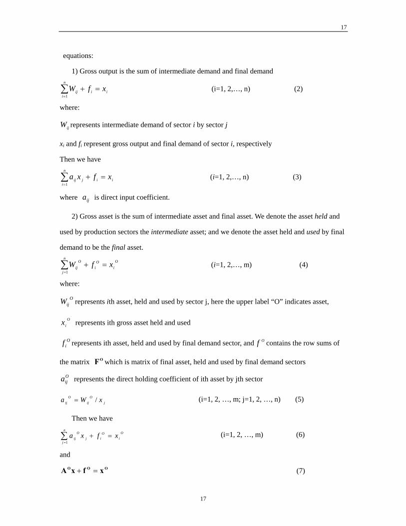
17

equations:

1) Gross output is the sum of intermediate demand and final demand

ii

n

iij xfW =+∑

=1 (i=1, 2,…, n) (2)

where:

ijW represents intermediate demand of sector i by sector j

xi and fi represent gross output and final demand of sector i, respectively

Then we have

ii

n

ijij xfxa =+∑

=1 (i=1, 2,…, n) (3)

where is direct input coefficient. ija

2) Gross asset is the sum of intermediate asset and final asset. We denote the asset held and

used by production sectors the intermediate asset; and we denote the asset held and used by final

demand to be the final asset.

Oi

Oi

n

j

Oij xfW =+∑

=1 (i=1, 2,…, m) (4)

where:

OijW represents ith asset, held and used by sector j, here the upper label “O” indicates asset,

Oix represents ith gross asset held and used

Oif represents ith asset, held and used by final demand sector, and contains the row sums of

the matrix which is matrix of final asset, held and used by final demand sectors

Of

OF

Oija represents the direct holding coefficient of ith asset by jth sector

jO

ijO

ij xWa /= (i=1, 2, …, m; j=1, 2, …, n) (5)

Then we have

Oi

Oi

n

jj

Oij xfxa =+∑

=1

(i=1, 2, …, m) (6)

and

OOO xfxA =+ (7)

17

18

Where

}{ Oija=OA

,{ 1= O ffOf

indicates direct holding coefficient matrix of asset

represents vector of final asset which is held and used by final demand

sectors.

},,2 ′Om

O fL

On the basis of this extended input-output model we will have some new concepts, models,

and calculation formulae—for example, total input coefficient with inputs of fixed assets, total

labor consumption coefficient, and total holding coefficients of fixed assets, financial assets,

natural resources, and labor.

2.3. Total Input Coefficient with Indirect Input of Fixed Assets

In input-output analysis, the standard static model can be expressed as

xfAx =+ (8)

Then we have

fIBfBfAIx )()( 1 +==−= − (9)

where:

1)( −−= AIB is the matrix of total requirements coefficients, or Leontief’s Inverse

IAIB −−= −1)( is the matrix of total input coefficients, or matrix of total consumption

coefficients, which are equal to the sum of direct input coefficient and total indirect input

coefficients. Element (i, j) of the Leontief inverse gives the output in sector i that is

required to satisfy a one unit final demand in sector j. The consumptions or inputs from sector i

that are required (directly and indirectly) in satisfying this one unit final demand in sector j are

given by element (i, j) of the matrix . The

difference between Leontief’s Inverse and matrix of total consumption coefficients is unity matrix

(final demands).

1)( −− AI

A +=−1) IAIAAAIAB −−=++−= −132 )(...(

The total consumption matrix is widely used in China, for example, to calculate total

18

19

electricity consumption of steel and calculate total labor consumption per ton of grain, etc. In the

above formula, a question arises concerning the calculation of total input coefficients. The

equations in B did not include the indirect consumption from the fixed assets. For example, if j

denotes steel, i denotes electricity, in the production of steel, some parts of factory buildings and

metallurgical equipment are consumed. The production of these buildings and equipment also

consumes electricity, which is obviously an indirect input of electricity to steel, but it is not

contained in the total consumption (total input) of electricity to steel in the normal input-output

model. Consequently, the total consumption coefficients derived from the above formula are

incomplete.

In order to completely include the indirect input of electricity via the fixed assets, a new

equation for computing the total input coefficients is developed by extended input-output model

with assets as follows (Chen, 1990).

*

1

*

1

***sjs

n

sis

n

kijikjikijij dbdabab αα ∑∑

==

+++= (i, j=1,2,…,n) (10)

In above equations, the first item in the right side of the above equations denotes direct

electricity consumption coefficient of electricity by steel, the second item denotes indirect

electricity consumption via intermediate input, the third one represents direct electricity

consumption via fixed assets which is equal to the product of depreciation rate and fixed asset

holding coefficient , and the last one represents indirect electricity consumption via fixed

assets. Because we haven’t data on actual consumption rate of fixed assets and only have

depreciation rate, we made an important assumption that the consumption rate of fixed asset

reflects or approximately equals to the depreciation rate of fixed assets. Then we have

iα

*ijd

DαBDαABAB ** ˆˆ* +++= (11)

Where:

*B represents a matrix of total input coefficients with the input of fixed assets

D a matrix of direct holding coefficients of fixed asset. D is the submatrix of direct holding

coefficients matrix that corresponds to the submatrix for fixed assets. OA

19

20

{ }iα=α̂ , represents a diagonal matrix of depreciation rates of fixed assets.

Therefore we can get:

DαADαAIB* ˆ)ˆ( +=−− (12)

We can prove that the matrix )ˆ( DαAI −− is nonsingular and its inverse exists.

Consequently we have

IDαAIB* −−−= −1)ˆ( (13)

It means that in above formula the matrix A is to be replaced by , and similarly B

by . The total input coefficients

DA α̂+

IDAI −−− −1)ˆ( α *B computed from (13) are obviously

greater than B. For example: Based on the extended input-output table for the urban and rural

economies of China in 1987, the total input coefficients of electricity to rice, coal, and

metallurgical industries were, respectively, 0.01810, 0.08019, and 0.08626 by use of B; and those

by use of the new equation B* were, respectively, 0.02045, 0.09334, and 0.09475.

What does it imply for the basic accounting equations of input-output table? The new

equations of the input-output table will be as follows

*fDxαAxx ++= ˆ (14)

and we have

*1)ˆ( fDαAIx −−−= (15)

Where

Dxαff * ˆ−= represents vector of net final demand, which is equal to the vector of final

demand minus vector of depreciation of fixed assets,

Under the following condition that vector of depreciation of fixed assets reflects or

approximately equals to the replacement of fixed assets, then reflects the vector of net final

demand, excluding replacement investment of fixed assets. In this case would then include the

net investments (gross investments minus the investment for replacement of fixed assets). Of

course, if data are available with respect to such replacement investments, then we could define

Dxα̂*f

*f

20

21

vector α̂ as diagonal vector of replacement rate of fixed assets. In this case it is assumed that

the consumption of fixed assets reflects or approximately equals to the replacement of fixed

assets3.

−A

2.4. Using an Extended Input-Output Model with Assets to Calculate Total Labor Consumption

Coefficient and Others

Total labor consumption coefficient is the sum of direct and indirect labor consumption per

unit product. It is a very important indicator to express social productivity for each sector. As we

know in the common input-output analysis, if the direct labor input coefficients are given by the

row vector , the ith element of the row vector l′ 1)( −−′=′ AIlµ gives the total amount of labor

that is (directly and indirectly) required to satisfy one unit of final demand in sector i.

The above formula of total labor consumption coefficient does not include labor consumed

by fixed assets. To overcome the problem, the new formula by the extended model with assets is

. 1)ˆ( −−′ DαIl

Similar results are obtained if the row vector with direct energy coefficients is replaced by a

vector with direct energy consumption coefficients, direct service input coefficients, direct water

input coefficients, direct input coefficients for employees’ compensations, direct input coefficient

of net indirect taxes, and others.

The above method could be used in many issues. For example, the traditional method of

calculating total service intensities of different industries is 1)( −−′ AIs

1)ˆ −− Dα

(Bhowmik, 2003). The

new formula to calculate total service intensities is . The difference between the

above two methods is that second one includes the indirect service input, contained in the fixed

assets.

( − AI

2.5. Using the Extended Input-output Model with Assets to Calculate Total Holding Coefficient of

3 From comments of Dr. Erik Dietzenbacher.

21

22

Asset and Others

Direct holding coefficient of asset is the ratio of ith asset divided by the output of sector j. It

indicates the holding intensity of ith asset by production sector j.

Oija

jO

ijOij xWa /= (16)

It can be written in matrix form

1ˆ −= xWA OO (17)

where:

OW indicates intermediate asset matrix

The total holding coefficient of asset can be calculated by two methods. The first one is: OB

1)( −−= AIAB OO (18)

The second method for calculating the total holding coefficient matrix of asset follows:

1* )ˆ( −−−= DαAIAB OO (19)

The total holding coefficient matrix could be used to calculate total holding intensity of fixed

assets, inventory, financial assets, employment, natural assets and others for unit of final demands.

For example, we use total holding coefficient matrix of employment to estimate the increase in

employment in the People’s Republic of China in response to an increase in exports from China

to United States.

2.6. Dynamic Extended Input-output Model with Assets4

Above we introduced the static extended input-output model with assets. In this part we

will discuss the dynamic extended input-output model. The Leontief dynamic

input-output model can be written as follows (Leontief, Chenery, Clark, Duesenberry,

Ferguson, Grosse, A. P., Grosse, R. N., Holzman, Isard, & Kistin, 1953):

4 We will discuss application of the dynamic extended I-O model in other paper.

22

23

fxCAxx ~=−− & (in continuous form) (20)

fxxCAxx ~)]()1([)()( =−+−− tttt (in discrete form) (21)

where:

C is a matrix of capital coefficient

f~ is a column vector of net final demands excluding capital formation

dtd /xx =&

The time lag in the above models is one year. These models reflect the relationships

between capital demand for increase in outputs in a later period (t+1 year) and products

use in the current period (t year).

Two issues arise:

1) In order to expand production, not only more fixed assets and inventory, but also

more labor, particularly skilled labor, are required.

As Schultz has indicated, humans are the determinant factor of production, and in

order to develop production it is first required to raise people’s cultural, scientific, and

technological knowledge. He put forward an important conception of human capital,

investment in increasing human capability, and also said that knowledge is the most

powerful engine of production. Based on U.S. data, Schultz established that the

contribution of human capital to profits is greater than that of physical capital (Schultz,

1961).

In the dynamic extended input-output model with assets, we must take into account

the fact that it takes a longer time to train skilled labor than to prepare fixed assets and

23

24

inventory. Therefore, future demand for labor for expanding production should be linked

with current human capital investment. Then, we get a new dynamic extended

input-output model reflecting the relationship between human capital demand for

increase in outputs in later periods and input for training in the current period. We obtain

the following model:

fxHxCAxx ~=−−− && (22)

where H is the matrix of human capital coefficient, which is necessary for increasing unit

output in next period, and

LMH L= (23)

where L is marginal labor force coefficient matrix and ML is the input matrix for training

the labor force. The discrete form of the above model is:

)(~)]()1()[()()( ttttt fxxHCAxx =−++−− (24)

This dynamic model shows the functional relationship between uses of products in

the current period and the needed skilled labor and capital for an increase in output in the

next period. For simplicity’s sake, here we also assumed that the time lag is one year. If

the time lag is more than one year, we can obtain a system of high-order-difference

differential equations (in continuous form) or a system of high-order-difference equations

(in discrete form).

Because most asset elements have time-lag problems similar to that of human capital

formation, we can formulate the following dynamic extended input-output model with

assets:

24

25

fxCAxx ~* =−− & (in continuous form) (25)

fxxCAxx ~)]()1([)()( * =−+−− tttt (in discrete form) (26)

where C* is the sum of matrix of marginal capital coefficient C, matrix of human capital

coefficient H, and others.

2) Leontief’s dynamic model does not include the requirement to cover consumption

of fixed assets.

From Leontief’s dynamic model, it can be seen that if production is not

expanded—that is, if =0, or x(t+1)-x(t)=0—then investment is not needed; in the real

world, however, gross capital formation is used not only to expand production, but also

for maintenance, i.e. to cover the consumption of existing assets (see Table 4).

x&

[TABLE 4 ABOUT HERE]

From Table 4 we can conclude that in China, Japan, and the United States the ratios of

depreciation of fixed assets on gross capital formation are very high: 36.2% in China

(1997), 72.4% in Japan (2000), and 70.3% in the United States (1990). In the last two

countries, most gross capital formation is to cover the consumption of fixed assets. This

ratio tends to increase over time. In Japan, it was 33.0% in 1960, 40.6% in 1980, 52.2%

in 1990, and 72.4% in 2000. This should not be ignored. This is for us an additional

motivation for extending the Leontief dynamic model as follows:

fxCxAαAxx ~ˆ =−−− &OCap (27)

where indicates average capital coefficient matrix, and OCapA

25

26

1ˆ −= xWA OCap

OCap (28)

where is the matrix of intermediate capital assets. If we assume that the average

capital coefficient is equal to the marginal capital coefficient, then equals to C, and

we have

OCapW

OCapA

fxCCxαAxx ~ˆ =−−− & (29)

We could get a dynamic model in discrete form as follows:

)(~)]()1([)(ˆ)()( tttttt fxxCCxαAxx =−+−−− (30)

Because labor eventually retires and this has to be put in a dynamic model, we put

forward an extended dynamic input-output model with assets on human capital as

follows:

fxHHxαxCCxαAxx ~ˆˆ =−−−−− && H (31)

where is diagonal matrix of labor retirement coefficients. We have the model in

discrete form:

Hα̂

)(~)]()1()[()()ˆˆ()()( tttttt H fxxHCxHαCαAxx =−++−+−− (32)

Because consumption of most assets must be covered, we have the following dynamic

extended input-output model:

fxCxCαAxx ~ˆ *** =−−− & (33)

where and α are the asset coefficient matrix for all occupied elements and the

diagonal matrix of consumption coefficient for all elements, respectively. The discrete

form of the above model is:

*C *ˆ

26

27

)(~))()1(()(ˆ *** tttt fxxCxCαAxx =−+−−− (34)

3. Yearly National Grain Output Prediction for China 1980–2004

Up to the present, the extended input-output model with assets has been used in China for grain

output prediction (Chen, Pan, Yang, 2001); to study the key sectors of Chinese economic

development in urban and rural economies, to calculate the amount of surplus labor

(unemployment) in rural areas (Chen, Cao, Xue & Lu, 1992); to predict, from a 1987 base,

economic development indicators in Xinjiang in 1990, 1995, and 2000 and to study relations

between Xinjiang and other regions of China; to study Shanxi Water Resource (Chen, 2000); to

study water conservancy for the nine major river basins in China (Chen, Yang and Xu, 2002); to

study Township and Village Enterprises (TVE) in China, in particular their coal and energy

utilization and environmental pollution (Yang, 2001). We will focus below on the example of

grain production.

3.1. Three Approaches to Predicting Grain Output

Feeding 1.2 billion citizens is a critical issue for China. At the end of 1970s, the former Rural

Development Research Center under the State Council requested that the Chinese Academy of

Sciences forecast national grain output with two preliminary requirements. First, the prediction

lead time should be half a year prior to harvest season so as to plan storage, imports, exports and

grain consumption as early as possible. Second, the prediction should be highly accurate, with an

error rate lower than 3%.

Three main approaches to predicting cereal output used worldwide are:

a. Meteorological approach, in which the main variables are temperature, sunshine, rainfall,

and so on.

b. Statistical dynamic simulation approach to studying relationships between grain yield and

effects of environmental factors such as temperature, sunshine and concentration of CO2 on crop

photosynthesis, transpiration, respiration, solid material and seed formation.

c. Remote sensing approach.

27

28

These approaches normally have a 5–10% error rate compared to reported output and a

two-month prediction lead time. For example, Williams, Joynt & Mecormick (1975) adopted the

meteorological approach to predicting Canadian prairie crop district cereal yields at the end of

June, two months prior to harvest, with an error rate of 8.8%, 4.7%, and 5.4% for wheat, oats, and

barley, respectively. Hayes and Decker (1996) used the Vegetation Condition Index derived from

NOAA/AVHRR (National Oceanographic and Atmospheric Administration/Advanced Very High

Resolution Radiometer) satellite data since 1982 to estimate maize production in corn belt of the

United States of America. The forecasting results from 1985 to 1992 had a lead time of about two

months and a 4.9% average error rate over the eight years, of which the rate was below 5% for

four years, 5–10% for three years, and higher than 10% for one year. (As we shall see later,

however, remote sensing provides the most accurate information about cultivated land which we

can use in our own predictions).

These approaches could not, however, satisfy the above two requirements of the Chinese

government of prediction lead time and accuracy.

3.2. Systematic Integrated Approach

The above approaches predict grain output mainly by meteorological factors. Up to the present it

has been extremely difficult to predict the weather—temperature, sunshine, rainfall, and so

on—two to three months away. In the late 1970s we suggested predicting grain output mainly by

factor input and assets, held and used, and presented a systematic integrated approach using the

key methods of an extended input-output model with assets, nonlinear variable coefficient

forecasting equations, and minimum sum of absolute value technique. Our theoretical

assumptions were as follows:

Agricultural production is a typical complex system with a multi-level structure. There are

complex interrelations between its subsystems and between the system and the external

environment, and the characteristics of the system are nonlinear, stochastic, and dynamic.

Grain output is affected by different types of factors: 1) social, economic, and production

technology factors, such as agricultural policies, education level of peasants, prices, fertilizers,

28

29

improved seed varieties, irrigation, machinery; 2) natural factors such as meteorological and

non-meteorological factors; 3) others. Only when we consider all these factors can we effectively

increase the accuracy of prediction of grain output.

The first set of factors, i.e. social, economic, and production technology factors, however,

play the critical role in increasing grain output. While the grain output of China in 1952 was

163.9 million tons, in 1998 it was 512.3 million tons. Over 46 years, the changes in China’s

meteorology were not striking to the same extent. Therefore, the increase in grain output is more

likely to have been caused mainly by changes in social, economic, and production technology

factors. These factors not only determine the long-term trend of grain production but are also a

major cause of yearly fluctuations in grain production. There are two periods of significant

variation in grain output since 1949: a drastic decline from 1959 to 1961, and a sharp increase

from 1981 to 1984, both of which were mainly caused by social, political, and economic factors.

The systematic integrated approach we proposed is based on synthetic method and

multi-equations forecasting model. In the approach we use extended input-output model with

assets, nonlinear forecasting equations and minimum sum of absolute value technique.

3.3. Extended Input-output Model with Assets on Chinese Agriculture

With the support of the former Rural Development Research Center of the State Council of China,

the Chinese Academy of Sciences and National Natural Science Foundation of China, the

Institute of Systems Science, we constructed an extended input-output table with assets in

agriculture for 1982 (Chen, Hao & Xue, 1991), 1984, 1987 (Chen, Cao, Xue & Lu, 1992), 1992,

and 1997. In other years, in order to predict output of grain, cotton, and oil-bearing crops we did

some updating calculations on the basis of these extended input-output tables.

The 1997 extended input-output table with assets on agriculture was constructed on the basis

of the 1997 national input-output table, compiled by the National Bureau of Statistics. For the

purpose of grain output prediction, in our extended input-output table with assets, the agriculture

industry was divided into the following 12 sectors: rice, wheat, corn, other grain, oil-bearing

29

30

crops, cotton, vegetables, other farm crops, forestry, livestock and livestock products, fishery, and

other agriculture. In China the term “grain” is the sum of rice, wheat, corn and other grain. Some

sectors, including grain, cotton, and oil-bearing crops, and some important agricultural inputs,

such as fertilizer and electricity, are measured not only in value, but also in physical units. There

are eight items in the asset part: sown area, cultivated land, irrigated area, labor, agricultural fixed

assets, total power of agricultural machinery, large and medium tractors, and mini-tractors. The

assets part of agriculture in the 1997 extended input-output table with assets is shown in Table 5.

[TABLE 5 ABOUT HERE]

Land and water play a very important role in grain production. The figures for cultivated land

prior and including 1995, published by the National Bureau of Statistics (NBS) of China, however,

were underestimated and cannot be used in our calculation. To date, we have only reliable figures

on cultivated land for 1996 and 2001, published by the NBS on the basis of the remote sensing

approach. In our grain output prediction, sown area of crops is a very important indicator. Grain

output is a function of the area sown in grain and grain yield. Therefore, if we had not taken

into consideration this asset, our predictions would necessarily been way off the mark. The

main cause of the sudden decline in grain output from 1999 to 2003 is the sharp drop of area

sown in grain (see Table 6).

[TABLE 6 ABOUT HERE]

From Table 6 we find that from 1998 to 2003 grain output in China dropped very quickly,

from 512.3 million tons to 430.7 million tons, or 15.9%. Areas sown in grain over the same

period fell from 113.787 million hectares to 99.410 million hectares, a drop of 12.8%, while grain

yield decreased by 3.8%. Thus, the sharp drop in Chinese grain output from 1998 to 2003 was

caused mainly by the decline in sown area.

Using data in the asset part of our extended input-output model, we calculate many important

indicators, such as consumption of chemical fertilizer and electricity per hectare of sown area,

fixed assets per hectare of sown area, ratio of irrigated area to cultivated area, labor per hectare,

total power of agricultural machinery per hectare, tractors per hectare, ratio of areas covered by

30

31

natural disasters to total sown areas, and ratio of total areas affected by natural disasters (natural

disasters include flood, drought, wind, hail and frost, etc.) to total areas covered by natural

disaster. In particular, we use the extended input-output model with assets to calculate the total

income per mu of sown area (1 hectare is equal to 15 mu) for grain and other important farm

crops (see Table 7), net income per workday, and profit rate of capital. Since 1981 China’s grain

output variation has had a close relationship with the variation of net income of grain. Because

the net income status of grain directly influences the quantities of factor inputs and holding of

asset in grain production, the net income of the previous year has a significant linear correlation

with the grain output of the current year.

[TABLE 7 ABOUT HERE]

According to our calculation and forecasting, the net income per mu of grain crops in 2004

will rise quickly and once again to a higher level than 1998. Using systematic integrated approach,

in April of 2004, we predicted and reported that grain output would rise and China would have a

good harvest in 2004. Using the extended input-output model with assets, the total consumption

coefficients of electricity, oil, and chemical fertilizer by grain crops can also be precisely

calculated. For example, the direct input of electricity for wheat was 68.1 kilowatts per ton; using

traditional formula of B, total consumption of electricity for wheat was 235.4 kilowatts per ton;

using formula (15), it was 268.6 kilowatts per ton. These results are important for our grain output

prediction.

3.4. Nonlinear Forecasting Equation with the Consideration of Diminishing Return

In fact, functional relationships between input and output, and between assets and output, are

usually nonlinear. For example, the effect of fertilizer on grain yield follows the law of

diminishing return to scale. Figure 1 shows that marginal product and average product per kg of

chemical fertilizer sharply decreases with increased consumption of chemical fertilizer per mu. To

improve forecasting accuracy, it is therefore necessary to construct nonlinear forecasting

equations.

[FIGURE 1 ABOUT HERE]

31

32

We have so far established 20 forecasting equations on grain yield with a high degree of

accuracy. These equations include different variables. Since the effect of fertilizers follows the

law of diminishing returns, it is shown as a nonlinear coefficient in the equations, for example:5

2001)-(1952 50N 1583; F0.9945;R(1.9588)

CA0.18578X (18.2190)

)]X(1.55-1.1).95e1.95153[(6(6.8073) (-3.8095) (3.8869) (10.3210) 1.44660X61.02954X-10.41246D62.27441ˆ

2

4

30.02X54X0.03911791-

21

33

===

++

+++

+++=Y (35)

where:

$Y : estimated grain yield per mu annually

D: annual policy dummy variable (D= -1 in case of negative agricultural policy such as which

resulted in the extensive loss of grain output during 1959–1961)

X1: ratio of areas covered by natural disasters on total sown areas

X2: ratio of irrigated area on cultivated area

X3: chemical fertilizer input per mu

X4: net income of grain per mu of the preceding year

CA: adjusted item

The above equation has the higher F value (F = 1583, R2 = 0.9945) and the reasonable t-test

values of fertilizer terms with an exponential form.

The nonlinear items of chemical and traditional fertilizer are calculated from historical data

on fertilizer inputs and yield increments, in particular statistically tested the data of yield

increments related to the increased chemical fertilizer inputs in some regions of China.

It is found in equation (35) that the t-test value of chemical fertilizer item is 18.2190. If we

did not consider the diminishing return, the t-test value would be only 0.4538; in other words,

there is no significant linear correlation between China’s grain yield and chemical fertilizer input.

6 Data in parenthesis are values of t-test.

32

33

3.5. Minimum Sum of Absolute Value Technique

In regression analysis, the parameter β is normally estimated by the least square (LS) method:

min ( $ ) Z Y Yi i= −∑ 2 (36)

The drawback is that the least square treatment will move the fitted curve to some

exceptional points, thus reducing forecasting accuracy. One of the modifications is to minimize

the sum of absolute value of errors between estimated and actual yields:

min ' | $ Z Yi= −∑ | (37) Yi

Equation (41) can be solved by the linear programming method. The model is as follows:6

(

2, , n

0

min ),

,

u vX X Y u v i

u v

i i

i k ki i i i

i i

+

+ + + − = − =≥ ≥

∑β β β1 1 1

0 0L L (38)

Following is the modified result of equation (39) by minimum sum of absolute value

approach:

19468.0)]X(1.55-1.1).95e2.01756[(6+ 29494.138615.9622152.1108731.67ˆ

430.02X54X0.03911791-

21

33 CAXXXDY

+++

++−+= (39)

This equation reduced the average error of grain yield per mu from 3.688 kg to 3.551 kg, and

the average error rate (average error over average yield) from 2.02% to 1.94%. The technique

also marginally improves the accuracy of the grain output prediction.

In order to increase forecasting accuracy, our research team also conducts field studies in the

13 main grain-production provinces in China in March and April of every year. We consult local

and national experts and gather their views (using a Delphi method) and collect other related

information, do technical and economic analysis, and then modify the results derived from

forecasting equations. In particular, we modify the adjusted item CA based on data from

experimental regions in response to unprecedented factors such as the Household Contract

Responsibility Policy System and new improved grain varieties.

6 It can be simply proved that uivi = 0, if optimal solution exists.

33

34

Besides, we use formulae (13) and (19) to calculate total requirements of chemical fertilizer

(electricity, diesel oil, etc.) and total requirements of various assets (fixed assets, land, water

resource, etc.), respectively. If current qualities of fertilizer and assets are not assured, the

predicated amount of grain output will be decreased.

From above description we could find that in systematic integrated approach mainly used

three methods: econometrics, extended input-output model with asset and mathematic

programming. In the approach extended input-output model is the basis to use other two methods.

Particularly, net income per mu of grain crops, which is calculated by the extended input-output

model, plays a key role in the grain output prediction. The assets which listed in the extended

input-output model are prerequisite and constraints for the grain production. Three methods are

used together. As Richard Stone said: “The development of the I/O model seems to be leading in

direction which its I/O core is becoming less and less discernible” (Stone, 1984).

3.6. Application and Evaluation

This approach has been successfully used in China since 1980. Every year at the beginning of

May, we send a report predicting national grain output to government agencies and top leaders of

China. From 1980 to 2003 the main results are as follows: Predicted bumper, average, and poor

harvests are correct every year. The prediction lead-time is more than half a year. Since 70% of

the grain is reaped in the fall and the harvest is over in November, a forecasting report at the end

of April provides government agencies with enough time to arrange for storage, imports, exports

and grain consumption. The forecasting accuracy was acceptable (under 3% error) for 19 years

out of 23. Over the period, error rates have been below 1% for eight years, 1–2% for six years,

2–3% for five years, 3–5% for two years, and 5–8% for two years. Overall, the average error rate

over 23 years is only 1.9% compared to statistical reports from sample surveys.

This forecasting has supported some important policy decisions. Given the predicted bumper

harvests of 1996, 1997, and 1998, the Chinese government and the China Agricultural Bank gave

financial aid to grain enterprises to expand their storage capacities. The relevant departments of

34

35

the Chinese government, such as the State Grain Administration, the Ministry of Agriculture, the

Research Department of State Council, and the National Development and Reform Commission

paid much attention to our predictions. For example, State Grain Administration wrote in the

documents: “lead time of prediction is very long”, “forecasting is accurate and prediction on the

grain situation is correct”, “supply very important reference to our Administration and others for

policy-making on grain supply and sale, grain imports and exports etc.” 7

9. Conclusions

The holding and using of assets is a prerequisite for production. Production in modern society

cannot occur without appropriate quantities of fixed assets, natural resources, labor, and financial

assets. The scale of production and the economic benefits derived from the output also partially

depend on the quality and quantity of production factors and assets. The output is obtained not

only by factor input, but also by assets held and used. The input-output model extended to assets

is a very important tool for analyzing the relationships between sectors.

Our contribution has been to formally incorporate assets into the input-output table and

establish a corresponding model system to calculate total input coefficient and related indexes, for

example, total coefficient of fixed asset. Most important, we have successfully applied this

method in predicting China's grain output from 1980 to 2004.

In the 1980s, when we wanted to predict annual grain output in China, we discovered it was

necessary to include assets in the input-output model. Since 1987, the model has been used in

China to analyze many issues. Most of published papers and books are in Chinese. Therefore

most input-output analysts in the world are as yet unaware of this extended input-output model to

assets, or its applications.

7 The work was awarded with the First Prize for Operational Research in Development in the 15th IFORS

Triennial Conference in 1999 (Chen, Pan & Yang, 1999). It was also awarded with the Outstanding Science

and Technology achievement Prize of the Chinese Academy of Sciences in 2003.

35

36

References

Almon, C. (1970) Investment in input-output models and the treatment of secondary products, in:

A. P. Carter and A. Bródy (eds) Contributions to Input-output Analysis (Amsterdam,

North-Holland Publishing).

Bhowmik, R. (2003) Service intensity in the Indian economy: 1968/9-1993/4, Economic Systems

Research, 15, pp.427-437.

Carter, A. P. (1970) Structural Change in the American Economy (Cambridge, MA, Harvard

University Press).

Chen, X. (1989) Input-output techniques in China, Economic Systems Research, 1, pp. 87–96.

Chen, X. (1990) Input-occupancy-output analysis and its application in China, in: M. Chatterji &

R. E. Kuenne (eds) Dynamics and Conflict in Regional Structural Change (London,

Macmillan), pp. 267–278.

Chen, X. (1998) Input-occupancy-output analysis and its application in Chinese economy,

International Journal of Development Planning Literature, 13, pp. 105–134. The paper is also

in: S. Dahiya (ed), The Current State of Economic Science (Rohtak, Spellbound Publications),

Vol. 1, pp. 501–514.

Chen, X. (2000) Water resource input-occupancy-output table and its application in Shanxi

Province of China, International Journal of Development Planning Literature, 15, pp. 247–264.

Chen, X. (2001) Input-occupancy-output table of foreign trade of China for 1995 and its

application, in: X. Xu & Q. Liu (eds) Input-Output Theory and Practice in China (Beijing,

China Statistical Press), pp. 185–192.

Chen, X. Cao, J., Xue X., & Lu Z. (1992) Input-Occupancy-Output Analysis of the Urban and

Rural Economies of China (Beijing, Science Press) (in Chinese).

Chen, X., Hao, J., & Xue, X. (1991) Application of the input-output table for agricultural sectors,

in: K. R. Polenske & X. Chen (eds) Chinese Economic Planning and Input-Output Analysis

(Hong Kong, New York, Oxford University Press), pp. 109–124.

Chen, X., Pan, X., & Yang C. (2001) On the study of China’s grain prediction, International

36

37

Transactions in Operations Research, 8, pp. 429–437.

Chen, X. & Xue, X. (1984) A non-linear input-output model in physical units and its application

in China, in: United Nations Industrial Development Organization (ed) Proceedings on the

Conference on Input-Output Techniques (New York, United Nations), pp. 201–209.

Chen, X., Yang C. & Xu J. (2002) Water conservancy economy input-occupancy-output table of

China and its application, International Journal of Development Planning Literature, 17(1–2),

pp. 19–28.

Department of Price, National Development and Reform Commission (2002, 2003 and 2004)

Compilation of Data on Costs and Benefits of Main Farm Crops of China, 2002, 2003, 2004

(Beijing, China Price Publishing House).

Ghosh, A. (1964) Experiments with Input-Output Models (Cambridge, Cambridge University

Press).

Green, M. J. (1971) Investment matrices for plant and machinery: 1963 and 1968, in: Economic

Trends (London, H.M.S.O.).

Grossling, W. F. (eds) (1975) Capital Coefficients and Dynamic Input-Output Models (London,

Input-Output Publishing Company).

Hayes, M. J. and Decker, W. L. (1996) Using NOAA/AVHRR data to estimate maize production

in the United States Corn Belt, International Journal of Remote Sensing, 17(16), pp.

3189–3200.

Hicks, J.R. (1965) Capital and Growth (Oxford, Clarendon Press).

Japan Statistical Bureau (2003) Input-Output Table in Japan, 1995 and 2000,

http://www.stat.go.jp/english/data/io/1995/zuhyou/ and

http://www.stat.go.jp/english/data/io/2000/zuhyou/.

Kimio Uno (1989) Input-Output Table in Japan 1951–1985 (Tsukuba, Japan, Institute of

Socioeconomic Planning, University of Tsukuba).

Kuroda, M. & Nomura, K. (2003) Technological Change and Accumulated Capital: A Dynamic

Decomposition of Japan’s Growth (Japan, Keio Data Base, Keio Economic Observatory).

37

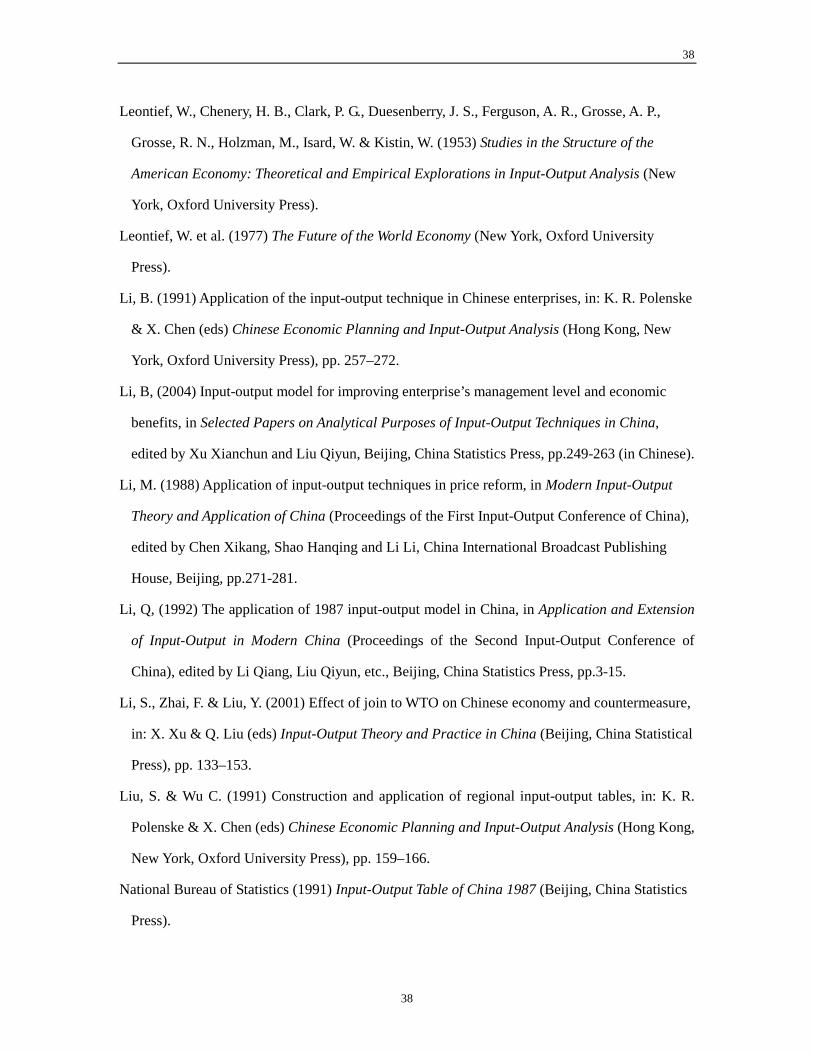
38

Leontief, W., Chenery, H. B., Clark, P. G., Duesenberry, J. S., Ferguson, A. R., Grosse, A. P.,

Grosse, R. N., Holzman, M., Isard, W. & Kistin, W. (1953) Studies in the Structure of the

American Economy: Theoretical and Empirical Explorations in Input-Output Analysis (New

York, Oxford University Press).

Leontief, W. et al. (1977) The Future of the World Economy (New York, Oxford University

Press).

Li, B. (1991) Application of the input-output technique in Chinese enterprises, in: K. R. Polenske

& X. Chen (eds) Chinese Economic Planning and Input-Output Analysis (Hong Kong, New

York, Oxford University Press), pp. 257–272.

Li, B, (2004) Input-output model for improving enterprise’s management level and economic

benefits, in Selected Papers on Analytical Purposes of Input-Output Techniques in China,

edited by Xu Xianchun and Liu Qiyun, Beijing, China Statistics Press, pp.249-263 (in Chinese).

Li, M. (1988) Application of input-output techniques in price reform, in Modern Input-Output

Theory and Application of China (Proceedings of the First Input-Output Conference of China),

edited by Chen Xikang, Shao Hanqing and Li Li, China International Broadcast Publishing

House, Beijing, pp.271-281.

Li, Q, (1992) The application of 1987 input-output model in China, in Application and Extension

of Input-Output in Modern China (Proceedings of the Second Input-Output Conference of

China), edited by Li Qiang, Liu Qiyun, etc., Beijing, China Statistics Press, pp.3-15.

Li, S., Zhai, F. & Liu, Y. (2001) Effect of join to WTO on Chinese economy and countermeasure,

in: X. Xu & Q. Liu (eds) Input-Output Theory and Practice in China (Beijing, China Statistical

Press), pp. 133–153.

Liu, S. & Wu C. (1991) Construction and application of regional input-output tables, in: K. R.

Polenske & X. Chen (eds) Chinese Economic Planning and Input-Output Analysis (Hong Kong,

New York, Oxford University Press), pp. 159–166.

National Bureau of Statistics (1991) Input-Output Table of China 1987 (Beijing, China Statistics

Press).

38

39

National Bureau of Statistics (1996) Input-Output Table of China 1992 (Value Unit) (Beijing,

China Statistics Press).

National Bureau of Statistics (1998) China Statistical Yearbook 1998 (Beijing, China Statistics

Press).

National Bureau of Statistics (1999a) Input-Output Table of China 1997 (Beijing, China Statistics

Press).

National Bureau of Statistics (1999b) Material of the National Economic Accounting in 1997,

unpublished data.

National Bureau of Statistics and State Planning Commission (eds.) (1984) Input-Output Table of

China 1981 (unpublished data).

National Development and Planning Commission, National Economic and Trade Commission,

Ministry of Agriculture, National Bureau of Forestry, National Bureau of Light Industry,

National Bureau of Tobacco and General Cooperative of Supply and Marketing of China,

Ministry of Foreign Trade and Cooperation (eds) (1998, 1999, 2000, 2001) Compilation of

Data on Costs and Benefits of Main Farm Crops of China for1988, 1999, 2000, 2001,

unpublished data.

OECD (2003) The OECD input-output Database, http://www.oecd.org/document

/6/0,2340,en_2825_495684_2672966_1_1_1_1,00.html/ and

http://www.oecd.org/EN/document/0,,EN-document-435-15-no-1-22204-435,00.htm/ .

Peterson, K. D. & Schott, K. (eds) (1979) The Measurement of Capital: Theory and Practice

(London, Macmillan).

Polenske, K. R. & Chen, X. (eds) (1991) Chinese Economic Planning and Input-Output Analysis

(Hong Kong, New York, Oxford University Press).

Rural Social and Economic Survey Team of National Statistical Bureau of China (1999, 2000,

2001, 2002, 2003): China Rural Statistical Yearbook for1999, 2000, 2001, 2002, 2003 (Beijing,

China Statistics Press).

Schultz, T. (1961) Investment in human capital, American Economic Review, 51, pp. 1–17.

39

40

Shen, L. and Wu, Z., 2004, Analysis on reasonability of the structure of foreign trade products, in

Selected Papers on Analytical Purposes of Input-Output Techniques in China, edited by

Xianchun Lu and Qiyun Liu, Beijing, China Statistics Press, pp.121-128 (in Chinese).

Stone, R. (1984) Where are we now? A short account of vthe development of input-output studies

and their present trends, in: United Nations Industrial Development Organization (ed)

Proceedings on the Conference on Input-Output Techniques (New York, United Nations), pp.

439-459.

Tong, R. & Wang, D. (1992) Application of input-output methods in cost calculation of enterprise,

in: Li, Q., Liu, Q., et al. (eds) Application and Extension of Input-Output Analysis in Modern

China (Beijing, China Statistics Press), pp. 355–365.

Williams, G. D.V., Joynt, M. I., & Mecormick, P. A. (1975) Regression analysis of Canadian

prairie crop district cereal yields, 1961–1972, in relation to weather, soil and trend, Canadian

Journal of Soil Science, 55, pp. 43–53.

Yang, C. (2001) Comparative analysis of investment effect between the TVEs and non-TVEs, in:

X. Xu & Q. Liu (eds) Input-Output Theory and Practice in China (Beijing, China Statistical

Press), pp. 180–184.

.Zhang, Y. & Zhao K. (2004) Compiling method and analytical application of China inter-regional

input-output tables, in Selected Papers on Analytical Purposes of Input-Output Techniques in

China, edited by Xu Xianchun and Liu Qiyun, Beijing, China Statistics Press, pp.224-235 (in

Chinese).

Table 1. Chinese national input-output tables, 1973–2000

Year Type of table Number of sectors/products Comments

1973 Physical 61 First national table (experimental) 1979 Physical

Value 61 21

1973 table updated by RAS method MBS table

1981 Physical Value

146 26

MBS table MBS table

1983 Physical Value

146 22

1981 updated physical table by RAS method1981 updated value table by RAS method

40

41

1987 Value 117 First table based on special input-output surveys

1990 Value 33 1987 updated table by RAS method 1992 Physical

Value 151 118

Tables based on special input-output surveys

1995 Value 33 1992 updated table by RAS method 1997 Value 124 Table based on special input-output surveys2000 Value 40 1997 updated table by RAS method

Source: Authors and Karen R. Polenske (Chen, 1989; Polenske & Chen, 1991) Note: MBS denotes Material Balance System.

41

42

Table 2. Extended input-output table with assets

Intermediate demand and intermediate asset

Final demand and final asset

Fixed capital formation

Changes in inventories

Sector 1 Sector 2 ⋯ Sector nX

Consum-ption 1, 2 ⋯ n 1, 2 ⋯ n

Exports Imports

Gross output and

gross assets

Sector 1 ⋯⋯

Inter- mediate input Sector n

W F x

Depreciation of fixed assets

Compensation of employees

Net indirect taxes

Primary Input

Operating surplus

V

FACTOR

I N P U T Total input x′

Sector 1 ⋯⋯ Fixed

Assets Sector n

Sector 1 ⋯⋯ InventorySector n

OW OF

Ox

Currency Deposits Loans Shares Security other than

shares Advances and trade

credits

H O L D I N G

FinancialAssets

Others

42

43

Illiterate Primary Junior secondary schoolSenior secondary schoolCollege

Labor

Higher level

Land Water resource Subsoil assets Forest

Natural Resources

Others

Patent Trade mark

A S S E T

IntangibleAssets Others

43

44

Table 3. A simplified form of the extended IO table with assets

Intermediate demand Final demand Gross outputs Intermediate inputs W F X

Primary inputs V

I N P U T Total inputs x′ Intermediate assets Final assets Gross assets

Fixed assets

Circulating assets OW 0F 0x

A S S E T Labor

Note: In China circulating assets includes financial assets in short term and inventory. The total circulating assets is estimated by the National

Bureau of Statistics in the national economic accounts. In statistical yearbook, published by the National Bureau of Statistics yearly, there are also figures of circulating assets of industry by sectors.

44

45

Table 4. The proportion of depreciation of fixed assets to gross capital formation in China, Japan and the United States

Unit: 1 billion respective currency units at current prices Gross capital formation

Total Gross

fixed asset formation

Depreciation of

fixed assets

Ratio of depreciation on

gross fixed asset formation

(%)

Ratio of depreciation on

gross capital formation (%)

China 1981 1987 1992 1997

151.7 437.3 963.8

2,845.7

118.9 380.3 831.7

2,515.4

41.1

120.2 353.7

1,031.2

34.6 31.6 42.5 41.0

27.1 27.5 36.7 36.2

Japan 1960 1970 1980 1985 1990 1995 2000

5,292.7

28,617.5 77,846.5 88,049.9

139,054.0 141,782.7 130,076.4

4,658.9

26,257.9 73,943.5 86,558.2

138,727.0 139,721.7 129,807.4

1,746.7 9,531.2

31,640.9 44,330.5 72,654.0 80,800.7 94,179.0

37.5 36.3 42.8 51.2 52.4 57.8 72.6

33.0 33.3 40.6 50.3 52.2 57.0 72.4

U.S. 1970 1980 1990

180.0 540.0 943.0

106.0 365.0 663.0

58.9 67.6 70.3

Sources: National Bureau of Statistics and State Planning Commission (1984); National Bureau of Statistics (1991,1996, 1999a); Kimio Uno (1989); Japan Statistical Bureau (2003); and OECD (2003).

45

46

Table 5. Asset holding part of agriculture in the 1997 extended IO table of China Crop cultivation

Grain crops Items Rice Wheat Corn Other

grainSub- total

Oil-bearingcrops

Cotton Vege- tables

Other farm crops

Sub- total

Forestry

Livestock and

livestock products

FisheryOther agri-

cultureTotal

Total sown area (1,000 ha)

31,765 30,057 23,775 27,315 112,912 12381 4,491 11,288 12,897 153,969 153,969

Area of cultivated land (1,000 ha)

23,059

25,385 21,080 24,345 93,869 11,805 3,638 7,870 12,376 129,558 129,558

Irrigated area (1,000 ha) 15,257 10,020 5,706 4,019 35,002 2,830 3,235 7,435 2,737 51,239 51,239Labor force (million

persons) 40.1 26.0 26.8 15.2 108.1 14.0 12.4 49.9 11.0 195.2 14.4 93.2 31.2 14.4 348.4

Total agricultural fixed assets (billion RMB)

92.8 77.2 49.2 9.5 228.7 18.5 12.6 90.5 28.2 378.5 29.0 191.4 94.9 28.8 722.6

Total power of agricultural machinery (million kW)

49.5 79.6 41.8 13.4 184.4 6.1 5.9 5.5 3.9 205.9 36.7 92.1 52.3 33.2 420.2

Large and medium tractors (1,000 units)

22.7 255.6 219.1 71.4 568.7 18.9 18.3 16.9 12.1 635.0 30.1 14.5 1.5 8.0 689.1

Mini-tractors (1,000 units)

2323 3737 1964 631 8654 288 279 256 185 9663 457 221 23 122 10485

Sources: National Bureau of Statistics (1998, 1999a, 1999b); National Development and Planning Commission, National Economic and Trade Commission, Ministry of Agriculture, National Bureau of Forestry, National Bureau of Light Industry, National Bureau of Tobacco and General Cooperative of Supply and Marketing of China, Ministry of Foreign Trade and Cooperation (eds) (1998). In the last source, there are many important figures per mu of sown area by major crops, for example, data on fixed assets depreciation cost, labor, cost of plows, cost of irrigation, taxes, benefits and others. These data are collected from surveys of 60,000 rural households in 1,300 counties in China.

Note: hectare is abbreviated as ha.

46

47

Table 6. Total sown area of farm crops, grain output, and grain yields in China, 1998– 2003

of which Of which

Year

Total sown area

in farm crops

(1,000 ha)

Grain crops Rice Wheat Corn

Other grain crops

Oil-bearing crops Cotton Vege-

tables Other farm

crops

Grain Output(million

tons)

Grain yields

(kg/ha)

1998 155,706 113,787 31,214 29,774 25,239 27,560 12,919 4,459 12,293 12,248 512.295 4502.21999 156,373 113,161 31,284 28,855 25,904 27,118 13,906 3,726 13,347 12,233 508.386 4492.62000 156,300 108,463 29,962 26,653 23,056 28,792 15,400 4,041 15,237 13,159 462.175 4261.22001 155,708 106,080 28,812 24,664 24,282 28,322 14,631 4,810 16,402 13,785 452.637 4266.92002 154,636 103,891 28,202 23,908 24,634 27,147 14,766 4,184 17,353 14,442 457.058 4399.4 2003 152,415 99,410 26,508 21,997 24,068 26,837 14,990 5,111 17,954 14,950 430.670 4332.3

Sources: Rural Social and Economic Survey Team of National Statistical Bureau of China (1999, 2000, 2001, 2002, 2003):. The 2003 figures are from Ministry of Agriculture of China.

Note: hectare is abbreviated as ha.

47

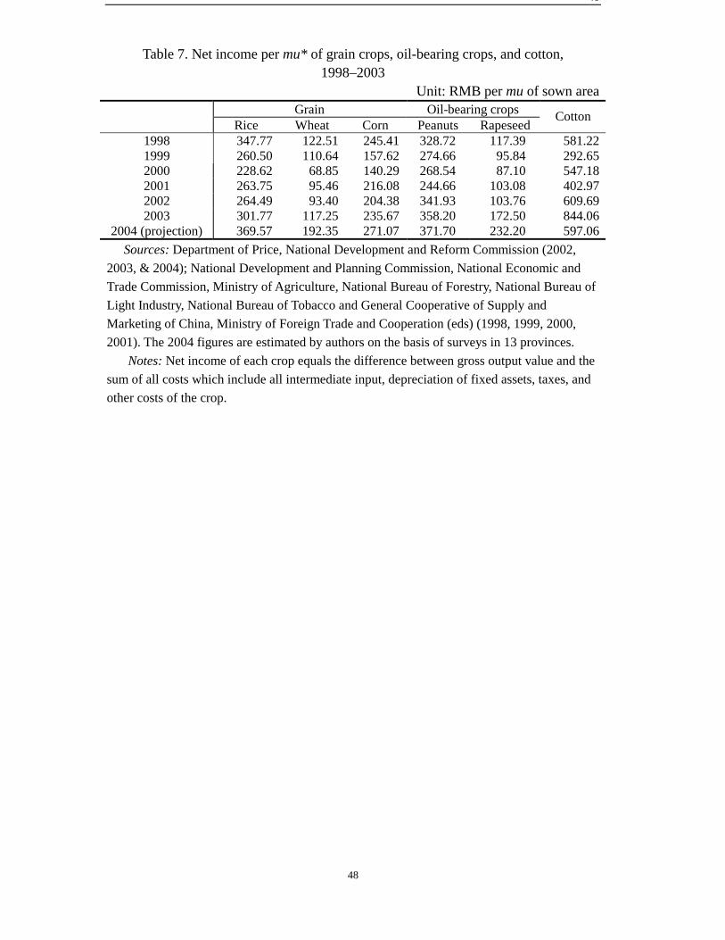
48

Table 7. Net income per mu* of grain crops, oil-bearing crops, and cotton,

1998–2003 Unit: RMB per mu of sown area

Grain Oil-bearing crops Rice Wheat Corn Peanuts Rapeseed

Cotton

1998 347.77 122.51 245.41 328.72 117.39 581.221999 260.50 110.64 157.62 274.66 95.84 292.652000 228.62 68.85 140.29 268.54 87.10 547.182001 263.75 95.46 216.08 244.66 103.08 402.972002 264.49 93.40 204.38 341.93 103.76 609.692003 301.77 117.25 235.67 358.20 172.50 844.06

2004 (projection) 369.57 192.35 271.07 371.70 232.20 597.06Sources: Department of Price, National Development and Reform Commission (2002,

2003, & 2004); National Development and Planning Commission, National Economic and Trade Commission, Ministry of Agriculture, National Bureau of Forestry, National Bureau of Light Industry, National Bureau of Tobacco and General Cooperative of Supply and Marketing of China, Ministry of Foreign Trade and Cooperation (eds) (1998, 1999, 2000, 2001). The 2004 figures are estimated by authors on the basis of surveys in 13 provinces.

Notes: Net income of each crop equals the difference between gross output value and the sum of all costs which include all intermediate input, depreciation of fixed assets, taxes, and other costs of the crop.

48

49

0

2

4

6

8

0 5 10 17 25 50Consumption of chemical fertilizer per mu of sown area

(kg/mu)

Gra

in o

utpu

t (kg

/mu)

10Marginal product Average product

Figure 1. Marginal product and average product per kg of chemical fertilizer in China

49