Children and Gender Inequality:

Evidence from Denmark∗

Henrik Jacobsen Kleven, London School of Economics

Camille Landais, London School of Economics

Jakob Egholt Søgaard, University of Copenhagen

March 2015

Abstract

Despite considerable gender convergence over time, substantial gender inequality persistsin all countries. Using Danish administrative data from 1980-2011, we show that most of theremaining gender inequality can be attributed to the dynamic effects of having children. Thearrival of children leads to a long-run penalty in female earnings of 21% driven in roughlyequal proportions by labor force participation, hours of work, and wage rates. Underlyingthis child penalty, we find clear dynamic effects of child birth on occupation, promotion tomanager, and the family friendliness of the firm for women relative to men. The fraction ofaggregate gender inequality that can be explained by children is strongly increasing over time—from 30% in 1980 to 80% in 2011—showing that non-child reasons for gender inequality havelargely disappeared. Conditional on rich observables, the female child penalty in earnings isincreasing in the relative skill of the female in the family, suggesting that mechanisms other thancomparative advantage are at play. We probe into the potential role of “gender identity” effectsby showing that the female child penalty is strongly related to the relative labor supply historyof her parents. This is consistent with the notion that gender attitudes surrounding family andcareer are shaped in part by the environment in which individuals grow up.

∗Kleven: h.j.kleven@lse.ac.uk; Landais: c.landais@lse.ac.uk; Søgaard: jes@econ.ku.dk. We thank Oriana Bandiera,Tim Besley, Raj Chetty, Marjorie McElroy, and Gilat Levy for helpful comments and discussions.

1 Introduction

Despite considerable gender convergence over the last century, substantial gender inequality per-

sists in all countries and the process of convergence has slowed down. The early literature on

gender inequality in the labor market focused on the role of education and discrimination (Altonji

& Blank 1999), but the disappearance of gender differences in education and the implementation

of anti-discrimination policies suggest that the explanation for the remaining gender gap lies else-

where. Based on administrative data for the full population in Denmark since 1980, we provide

a simple explanation for the persistence of gender inequality: the effects of parenthood on the

careers of women relative to men are large and have not fallen over time. Hence, most of the re-

maining gender inequality can be attributed to children. Our findings are surprising given that

Scandinavian countries have been leaders in the implementation of legislation and policies that

are supposed to allow women to balance career and family.

To provide context, Figure 1A shows the evolution of the gender gap in earnings for full-time

workers in different countries. It is striking that the cross-country differences in gender inequal-

ity have largely disappeared over time. For example, while gender inequality in Denmark was

dramatically lower than in the United States around 1980, today the gender pay gap is between

15-20% in both countries and appears to have plateaued at that level. That is, gender conver-

gence happened earlier in Scandinavia than elsewhere, but the process also slowed down earlier

in Scandinavia allowing other countries to catch up. So even though these countries feature differ-

ent public policies and labor markets, they are no longer very different in terms of overall gender

inequality.

To estimate the effect of parenthood on the careers of women relative to men, we adopt a

quasi-experimental approach based event studies around the birth of the first child. For a range

of labor market outcomes, we find large and sharp effects of children: women and men evolve in

parallel until the birth of their first child, diverge sharply immediately after child birth, and do not

converge again. The long-run child penalty in female earnings equals 21% over the period 1980-

2011. This should be interpreted as a total penalty that includes the costs of children born after

the first one, and we show that the penalty is increasing in the number of children. The earnings

penalty can come from three margins—labor force participation, hours of work, and the wage

1

rate—and we find sharp effects on all three margins that are roughly equal in size. Our ability to

precisely estimate hours and wage rate effects relies on a unique administrative and third-party

reported measure of working hours that is available for the full population.

Based on the event study approach, we find effects on several other margins that can shed light

on some of the underlying mechanisms. Just after the birth of the first child, women start falling

behind men in terms of their occupational rank (ordered by earnings level) and their probability

of being manager. Furthermore, women switch jobs to firms that are more “family friendly” as

measured by the share of women with young children in the firm’s workforce, or by an indicator

for being in the public sector which is known to provide very flexible conditions for working

women (see Nielsen et al. 2004). Since family friendly firms are associated with lower earnings and

wage rates, this response explains part of the gender gaps described above.

Having obtained micro estimates of child penalties in the full population—allowing for vari-

ation across birth cohorts—we are able to decompose aggregate gender inequality over time into

child-related inequality and residual inequality. We show that the fraction of total earnings in-

equality that can be explained by children has risen from 30% in 1980 to 80% in 2011. This dramatic

change reflects a combination of two effects: (i) the child-related earnings gap has increased from

about 14% to 18%, and (ii) the total earnings gap has fallen from about 45% to 22%.1 To under-

stand the first effect, note that although the female child penalty in percentage terms has fallen

slightly over time, the penalty operates on a larger base due to the general increase in the earnings

of women relative to men. Our findings have implications for future work on gender inequality,

which should focus on understanding what drives gender roles and gender outcomes in relation

to parenting. This is consistent with the views expressed by Goldin (2014) on what the “last chap-

ter” of gender convergence must contain, but the persistence of child penalties in a country with

generous family policies suggests that the last chapter may not be written any time soon.

Further insight can be obtained by analyzing the heterogeneity of child penalties across fami-

lies. This analysis shows that relative skill within families—as measured by relative wage rates in

the years prior to child birth—do not affect child penalties in the direction one might expect. Both

the earnings penalty and the wage rate penalty are increasing in the skill of the mother relative to

the father, conditional on a rich set of covariates. Even in families where the woman is the primary

earner before having children she takes the major hit when children arrives. These findings are

1These gender gaps are larger than those reported in Figure 1A discussed above. This is because the cross-countryevidence in Figure 1A is based on median earnings for full-time workers, whereas we are now considering mean earningsfor all workers as shown in Figure 1B.

2

interesting in relation to the evidence on the disappearance of the gender gap in education (Goldin

et al. 2006; Goldin & Katz 2008). While the closing of the education gap has a direct and positive

effect on gender equality in earnings (consistent with the reduction in non-child gender inequality

that we document), the potential gain will not be fully realized if child penalties are borne to a

larger degree by highly skilled women. The large child penalties for high-skill women that we

estimate are consistent with evidence for the US by Bertrand et al. (2010) and Wilde et al. (2010).

The size and persistence of female child penalties, along with their heterogeneity across skill,

are difficult to reconcile with comparative advantage alone. A recent literature discusses the im-

portance of social norms and gender identity for explaining the different labor market outcomes

of men and women, although causal testing of these ideas is difficult (Bertrand 2011; Bertrand

et al. 2013). We explore the potential role of such effects by showing that the female child penalty

is strongly related to the labor supply history of her parents, conditional on the socio-economic

characteristics of the family. For example, in traditional families where the mother works very

little compared to the father, their daughter pays a much larger child penalty when she eventually

becomes a mother herself. We estimate the intergenerational transmission of child penalties by ex-

ploiting that our administrative measure of hours worked goes back to 1964, allowing us to relate

the estimated child penalties between 1980-2011 to the within-family work history one genera-

tion before. Our findings are consistent with an influence of nurture in the formation of women’s

preferences over family and career. This analysis is related to the work by Fernandez et al. (2004),

but focusing on the intergenerational transmission of child penalties (as opposed to labor supply

levels) between parents and their daughters (as opposed to daughters-in-law).

Our paper speaks to the large literature on gender inequality in the labor market (reviewed

by Altonji & Blank 1999; Bertrand 2011), and it is closely related to a body of work emphasizing

the importance of parenthood for gender differences (e.g. Waldfogel 1998; Lundberg & Rose 2000;

Paull 2008; Bertrand et al. 2010; Wilde et al. 2010; Adda et al. 2011; Angelov et al. 2014; Goldin

2014). While some of the existing literature estimates child penalties using event study approaches

related to ours, we leverage the quality and comprehensiveness of the Danish administrative data

to document how micro-level child penalties translates into macro-level gender inequality over a

long time period. Although we find that child-related inequality is large and persistent, one could

argue that the event study approach represents a lower bound due to a potential effect of children

that it misses. If women select family-friendly career paths (offering flexible hours and generous

maternity leave, but lower wages) based on their planned fertility prior to child birth, then the

3

pre-child gender gap partly reflects a child penalty. This idea is consistent with our finding that

women are working in relatively family-friendly firms and sectors prior to child birth, and that

this by itself reduces the child penalty following child birth (see also Nielsen et al. 2004). From this

perspective our estimates may be viewed as conservative.

Our paper is also related to the literature on family labor supply and fertility. This literature has

tried to estimate the causal effect of children on female labor supply using potentially exogenous

variation in family size coming from twin births, sibling sex mix, miscarriage and infertility (see

e.g., Browning 1992; Bronars & Grogger 1994; Angrist & Evans 1998; Hotz et al. 2005; Aguero &

Marks 2008). The empirical approach in our paper is different from this body of work, and the

objective is different too. Our identification is based on sharp breaks in career trajectories that

occur just after having children for women, but not for men. These sharp dynamic patterns are

unlikely to be driven by omitted variables or selection on unobservables as these factors should be

smooth around the precise moment of child birth.

While we are thus capturing a causal effect of children on labor market outcomes, it is impor-

tant to keep in mind that having children is a choice and this affects the interpretation. In particular,

by estimating the relationship between children and career choices, our results are most naturally

interpreted as measuring complementarity in preferences. We show that this complementarity is

very strong for women but not for men, and that these gendered preferences can account for most

of the remaining gender inequality. The key question is why preferences are so strongly gendered.

Is it biology or is there a role for environmental influences in the formation of preferences? We

start probing into these questions by considering patterns of heterogeneity and intergenerational

transmission, but future work should go further in the investigation of the underlying mechanisms

as this will ultimately determine the welfare and policy implications of the patterns we uncover

here.

The paper is organized as follows. Section 2 describes the context and data, section 3 lays out

the event study methodology, section 4 presents the empirical results, and section 6 concludes.

2 Context and Data

2.1 Context

Scandinavian countries have been praised for offering better opportunities for women to balance

career and family than most other countries. This view is based on the presence of generous family

4

policies—job-protected parental leave and public provision of child care—and a perception that

gender norms are comparatively egalitarian in Scandinavia. Consistent with this view, Denmark

has one of the highest female labor force participation rates in the world, currently around 80%

as opposed to around 70% in the United States, and it has almost no remaining gender gap in

participation rates. However, Figure 1 shows that this is far from the full story. The cross-country

comparisons in Panel A were discussed above and shows that Denmark is no longer a strong

outlier in terms of the gender gap in earnings for full-time workers. Panel B focuses on Denmark

alone and shows gender gaps in different labor market outcomes for all workers. We see that the

gender gap in participation has gradually disappeared over the last three decades and that the

gender gap in hours worked has fallen substantially, but that large gaps persist in earnings and

wage rates (defined as earnings/hours worked among those who are working). The earnings gap

is now around 22% and is created mostly by differences in wage rates and to a smaller degree by

differences in hours worked.2

Figure 2 probes the idea that gender norms are more egalitarian in Scandinavia than elsewhere.

The evidence in the figure is based on questions from the International Social Survey Program

(ISSP) regarding the attitudes that people have towards market work by women with and without

children. Specifically the survey asks participants whether they think women should work outside

the home full-time, part-time or not at all when they have no children (Panel A), have children

under school age (Panel B), have children in school (Panel C), and have children who have left

home (Panel D). Two striking insights emerge from the figure: one is that gender attitudes are

still quite traditional—essentially that women should work full-time before having children and

after the children have left home, while they should work only part-time or not at all when they

have children living at home—and the other is that different countries are very similar in holding

this view. The only noticeable cross-country difference is that the Scandinavian populations are

somewhat more open to the idea that women with young children work part time (rather than

staying at home entirely) compared to the US and UK populations, but overall the similiarities

in gender attitudes stand out much more than the differences. The figure is based on samples

that include both men and women, but interestingly there is very little difference in these gender

attitudes between men and women. Overall and in contrast to common wisdom, the evidence

presented in Figures 1 and 2 raises doubts about the degree to which Scandinavian countries are

2As we describe below, the way we measure hours worked means that we understate somewhat the gender hoursgap and by implication overstate the gender wage rate gap. That is, the decomposition in Figure 1B of the earnings gapinto the underlying margins is tilted somewhat from hours worked to wage rates.

5

positive outliers in terms of gender equality in the labor market.

The policy environment in Denmark is one which combines large tax-transfer distortions (which

may affect the gender gap due to differential labor supply elasticities between men and women)

and generous family policies intended to support female labor supply. As shown by Kleven (2014),

the effective tax rate on labor earnings is exceptionally large in Denmark, but so are the implicit

subsidies to labor supply through publicly provided child care and public spending on other goods

that are complementary to working (transportation, elder care, education, etc.). Over the period

we consider, public child care is universally provided at a heavily subsidized price from around

6-12 months after birth. Until the child reaches the age where public child care becomes avail-

able, there is job-protected and paid maternity and parental leave. Up until 2001, parents were

offered 14 weeks of maternity leave followed by 10 weeks of parental leave to be shared between

the mother and father. Since 2002 this has been extended to 18 weeks of maternity leave and 32

weeks of parental leave. Hence, throughout the period we consider, parents were covered first by

paid leave and then by public child care, with no gap between the two.

2.2 Data

The analysis is based on administrative data for the full population in Denmark between 1980-

2011. For the study of intergenerational transmission we exploit additional administrative data

going back to 1964. The Danish data combines several different administrative registers (linked

at the individual level via personal identification numbers) and therefore contains rich informa-

tion on children, earnings, labor supply, occupation, firm, education, and many other outcomes.

Furthermore, the data allows us to link family members, generations, and workers to firms.

The Danish population is currently 5.5 million people and there were around 2 million child

births during the period 1980-2011. For our main event study analysis we focus on first child births

where both parents are observed every year between 5 years before having a child and 10 years

after. We are thus focusing on first child births between 1985-2001 where both parents are alive and

reside in Denmark throughout a 15-year window around the birth. We condition on both parents

being at least 20 years of age when having their first child (teenage births constitute only 2.3% of

all births during the 1985-2001 period). We do not impose restrictions on the relationship status of

the parents: we include all individuals who have a child together in a given year and follow them

through the 15-year window whether or not they are married, cohabiting, separated, divorced, or

have not formed a couple yet in any given year. This leaves us with a core estimation sample of

6

around 350,000 births or 11,200,000 individual-year observations.

We estimate child penalties in earnings, labor force participation, hours worked, and wage

rates (earnings/hours worked for those who are working). Our ability to estimate child penalties

in hours worked and wage rates using sharp event studies relies on a unique administrative and

third-party reported measure of hours worked that is available for the full population. This mea-

sure comes from a mandated pension scheme introduced in 1964—Arbejdsmarkedets Tillægspension

(ATP)—that require all employers to contribute on behalf of their employees based on individual

hours worked.3 The pension contribution is a function of hours worked in discrete steps, namely

four bins of weekly hours (0-8, 9-17, 18-26, 27-) for someone paid weekly or four bins of monthly

hours (0-38, 39-77, 78-116, 117-) for someone paid monthly, with the latter being much more com-

mon. Hence the annual pension contribution for someone paid monthly depends on ∑12i=1 hi where

monthly hours hi has 4 steps, which gives an annual hours measure in 37 steps (= 4 × 12 - 12 + 1).

Our measure of the wage rate is defined as earnings divided by this ATP hours measure.

Because the ATP hours measure is capped, it does not capture marginal hours adjustments

for those working every month of the year in the highest hours bin. For a given child penalty

in earnings, this will make us underestimate the penalty in hours worked and correspondingly

overestimate the penalty in wage rates. The hours measure does capture larger labor supply ad-

justments such as switches to different levels of part-time work and work interruptions within the

year, which are important adjustments for women with children. The key advantage of our mea-

sure is that it is precisely measured for the full population over a very long time period, unlike

labor market surveys that have considerable measurement error and small samples. Moreover, we

are able to validate our results for the discrete hours measure against a continuous hours measure

reported by all firms on behalf of their employees, but only since 1997.

3 Event Study Approach

The idea of the event study approach is to estimate female child penalties based on (sharp) changes

that occur just after child birth for mothers relative to fathers. For each parent in the data we denote

by t = 0 the year in which the individual has his/her first child and index all years relative to that

year. As described above, we consider a balanced panel of parents who we observe every year

between 5 years before having their first child and 10 years after, and so event time t runs from -5

3The scheme also covers self-employed individuals who contribute on their own behalf.

7

to +10. We then study the evolution of different outcomes (earnings, labor supply, wage rates, etc.)

as a function of event time.

Specifically, denoting by Yist the outcome of interest for individual i in year s at event time t,

we run the following regression separately for men and women

Yist = ∑t6=−1

αt ·EV ENTit + ∑j

βj ·AGEjis + ∑

s

γs · Y EARs + νist, (1)

where EV ENTit is an event time dummy, AGEjis is an age dummy for being j years old, and

Y EARs is a year dummy. We omit the event time dummy at t = −1, implying that the event co-

efficients αt measure the impact of children relative to the year just before the first child birth.

If we did not include the age and year dummies in the specification, the estimated event co-

efficients αt would correspond simply to the mean value of the outcome at event time t, mea-

sured relative to the year before birth. By including a full set of age dummies we control non-

parametrically for non-child related career progression, and by including year dummies we control

non-parametrically for non-child related time changes such as wage inflation and business cycles.

In other words, the age and year dummies remove any underlying life-cycle and time trends in the

outcomes we consider.

We specify equation (1) in levels rather than in logs to be able to keep the zeros in the data

(due to non-participation). We convert the estimated level effects into percentages by calculating

αt/E[Yist | t

]where Yist is the predicted outcome when omitting the contribution of the event

dummies, i.e. Yist ≡ ∑j βj ·AGEjis + ∑s γs · Y EARs. This captures the year-t effect of having a

child as percentage of the counterfactual outcome absent the child. We estimate this separately for

men and women and denote the gender-specific effects by P kt ≡ αk

t /E[Y kist | t

]where k = m,w.

We then define the long-run child penalty on women as the average effect of children over a 10-year

horizon for women relative to men, i.e.

∆P ≡ Pm − Pw where P k ≡ E[P kt | 0 < t ≤ 10

]. (2)

Hence, the child penalty ∆P is the percentage by which women are falling behind men due to

children over a 10-year period following the first child birth. The choice of a 10-year window is

based on the empirical analysis below, which shows that the effect is roughly at a steady state by

that time.

8

To gain insight into the potential determinants of child penalties, we present a detailed study

of heterogeneity using the rich observational data. Here we consider penalties at the family level

and regress these on a range of non-parametric controls. The long-run child penalty on the female

in family i is defined as

∆pi ≡ pmi − pwi where pki ≡E[Y kit | 0 < t ≤ 10

]−E

[Y kit | −5 ≤ t < 0

]E[Y kit | −5 ≤ t < 0

] , (3)

that is, the percentage change in a given outcome between the 5-year period before birth and the

10-year period after birth for the man relative to the woman within a family. The family-level

penalty in equation (3) is conceptually similar to the aggregate-level penalty in equation (2), but

in general it does not aggregate to the same number: the average over family-level penalties in

percentages (E [∆pi]) is not the same as the percentage penalty in the average levels (∆P ) due to

a potential correlation between penalties and the outcome level. Furthermore, when focusing on

family-level penalties, we have to drop families in which one or both of the parents have zeros

(non-participation) in all five years preceding the arrival of the child. The key advantage of defin-

ing family-level penalties is that it allows us to study heterogeneity in a given dimension while

controlling for the (correlated) variation in other relevant determinants of penalties.

We regress the penalty ∆pi on a range of variables that capture the socio-demographics, work

environment, and relative skill of the two parents in the family. The richest specification we con-

sider is the following

∆pi = ∑c

β1c ·COHORT ci + ∑

k∑j

β2jk ·AGEjki + ∑

j

β3j ·KIDSji + ∑

j

β4j · INCOMEji

+∑j

β5j ·EDUCATION ji + ∑

j

β6j · SKILLji + ∑

k∑j

β7j ·EXPERIENCEjki (4)

+β8 · PUBLICi + ∑j

β9j · FRIENDLY ji + ∑

k∑j

β10j · PROFESSION jki + µic.

The explanatory variables in (4) are dummies defined as follows: COHORT ci is a dummy for the

first child being born in year c, AGEjki is a dummy for parent k being j years old when having

the first child, KIDSji is a dummy for having j children in total (1, 2, 3, 4+), INCOMEj

i is a

dummy for being in the jth decile of the household income distribution just before having the first

child, EDUCATION ji is a dummy for being in the jth quartile of the distribution of relative years

of education between parents (based on completed education before having a child), SKILLji is a

dummy for being in the jth decile of the distribution of relative wage rates between parents (based

9

on the five years prior to having the first child),EXPERIENCEjki is a dummy for parent k having

j years of experience between completing education and the arrival of the first child (bottom coded

at zero if education is completed after child birth), PUBLICi is a dummy for the woman working

in the public sector at the time of having her first child, FRIENDLY ji is a dummy for the woman

working in a firm belonging to the jth quartile of the distribution of family friendliness when she

has her first child, and PROFESSION jki is a dummy for parent k being in profession j (based on

22 categories education fields). Family friendliness FRIENDLY ji is based on the share of women

with young children in the firm’s workforce (or by the presence of women with young children in

the firm’s management).

4 Empirical Results I: Child Penalties and the Gender Gap

4.1 Estimating Child Penalties

We start by documenting a set of stark changes in the labor market outcomes of women relative to

men around the event of having the first child. Figure 3 plots Pmt and Pw

t as defined in section 3:

these are outcomes for men and women as a function of event time t, measured relative to the year

just before the birth of the first child (t = −1) and controlling non-parametrically for age and time

trends. The figure includes 95% confidence bands around the event coefficients, although these

are not always clearly visible due to the enormous amount of precision in the administrative data.

Panel A starts by considering total earnings before taxes and transfers. We see that, once life-cycle

and time trends are taken out, the earnings of men and women evolve in a strikingly parallel way

until they become parents. But at the precise moment that the first child arrives, the earnings paths

of men and women begin to diverge: women experience an immediate drop in gross earnings of

almost 30%, while men experience no significant variation in their earnings. Importantly, in the

years following the initial drop, the earnings of women never converge back to their original level.

Ten years after the birth of a first child, female earnings have plateaued around 20% below its level

just before child birth, whereas male earnings are essentially unaffected by children. As shown in

the figure, these estimates imply a long-run child penalty in the earnings of women relative to men

(∆P defined in equation (2)) equal to 20.8%.

While we take an event study approach using the birth of the first child, the evidence presented

in Figure 3 is based on the full population of women with children, irrespective of the total num-

ber of children a woman ends up having. This implies that the dynamic patterns we document

10

include the effects of children born after the first one, and the estimated long-run child penalty is

naturally interpreted as the aggregate penalty of all children. In appendix Figure A.I we replicate

the earnings event study from Figure 3A for different numbers of children (1, 2, 3, 4+). The impact

of children is sharp for all four family sizes and the magnitude of the long-run child penalty varies

with the number of children in the expected direction. The child penalty increases by roughly 10

percentage points per child. Note that the event study graph for families with two children in

Panel B of Figure A.I looks very similar to the graph for all families in Figure 3, which is natural

given that the average completed fertility per woman in Denmark is close to two conditional on

having children.

In general, earnings responses can be driven by three margins: labor force participation, hours

worked conditional on participation, and the wage rate. In panels B-D of Figure 3 we analyze how

parenthood affects each of these three margins separately using the same methodology as above.

Panel B plots the evolution of hours worked for men and women relative to the year before the

first child birth. Hours worked follow the same qualitative pattern as earnings, with a sharp and

persistent drop after child birth for women relative to men. Three years after birth, hours worked

by women are 10% lower than before birth, while hours worked by men are almost unchanged. Ten

years after birth, there is no sign of convergence; a persistent 10% gender gap in hours worked has

been created due to children. Panel C displays the evolution of the labor force participation rates

of men and women. Again, the labor force participation trends of men and women are perfectly

similar until the birth of a first child, at which point they sharply diverge with a 10% relative drop

for women that fully persists over time. Finally, Panel D shows that wage rates feature a similar

dynamic pattern: men and women are on very similar trends prior to the birth of the first child,

diverge immediately after birth, creating a 10% gap between men and women that does not fade

over time.

These results show that the female child penalty in earnings is in part a direct consequence of

intensive and extensive labor supply adjustments made by the family after the birth of the first

child. At the same time, the wage rate patterns suggest that there is more going on than these

quantitative labor supply adjustments. A possibility is that women, once they become mothers,

make active career decisons in other more qualitative dimensions (choice of occupations, tasks,

firms) that have immediate and persistent effects on their wage rates. We provide direct evidence

on such margins of adjustment in the next section. Interestingly, the estimated long-run penalties

at the intensive, extensive, and wage rate margins are roughly similar in magnitude, suggesting

11

that these margins are equally important for understanding the long-run effect of children on the

earnings paths of women relative to men.4

In the event graphs presented so far, the drop in earnings and labor supply in event year 0 is

not much larger than the drop in subsequent event years. While this may seem surprising, note

that the use of calendar-year measures of earnings and labor supply tend to create attenuation bias

in the first-year dip compared to a continuous time representation: as women give birth some time

during year 0, some of the earnings and hours in calendar-year 0 were realized prior to child birth.

To investigate this point, we reproduce Figure 3 on a sample restricted to child births in January for

which the definition of calendar years and event years coincide. The results are shown in appendix

Figure A.II from which the following insights emerge. First, when focusing on January births alone

we do see a pronounced dip in event year 0 as one would expect. This dip reflects the extra time

taken out of the labor market immediately following delivery. Second, focusing on January births

also reveal a slight drop in labor market outcomes in event year -1, which can be explained by sick

leave and parental leave (for which women are eligible during the last four weeks of pregnancy)

taken just before giving birth. Third and most important, the long-run child penalties over a 10-

year horizon are very similar for January births and all births, which implies that the calendar-year

presentation in Figure 3 does not introduce any bias in the long run.

We have presented estimates on the career cost of children using child births between 1985-

2001 and an event study horizon that includes 10 post-birth years. It is of course interesting to

study how these career patterns evolve in the very long run, which is feasible to explore with our

data. In appendix Figure A.III we consider child births between 1985-1991 and a 20-year post-birth

horizon. The figure is otherwise similar to Figure 3 and shows results for earnings, hours worked,

participation, and wage rates. The long-run child penalty estimates shown in each panel is based

on an average over event years 10-20 (∆P in equation (2) for 10 < t ≤ 20). The figure shows how

strikingly persistent the effects of children are. In fact, the earnings penalty 20 years after child

birth is almost the same as the penalty 10 years after. The only qualitative difference that emerges

from considering the very long run is that hours worked do eventually begin to converge, while

at the same time wage rates keep diverging. The combination of the narrowing hours gap and the

widening wage rate gap produces a constant earnings gap.

It is useful to take a step back in order to discuss identification and how to interpret the event

4The child penalties in panels B-D of Figure 3 are unconditional penalties: when estimating the effect of parenthoodon one particular margin, we are not controlling for the other two margins in the regression. This explains why thelong-run penalties on the three margins do not sum up to the overall earnings penalty.

12

study estimates we have presented. Consider first the relationship between our approach and

the vast literature on family labor supply and fertility (e.g., Browning 1992). This literature has

discussed the difficulties of interpreting the observed negative correlation between children and

female labor supply, noting that causal inference is difficult due to omitted variables and reverse

causation. A series of papers try to estimate the causal effect of children on female labor sup-

ply using potentially exogenous instruments for family size such as twin births, sibling sex mix,

miscarriage, and infertility (e.g., Bronars & Grogger 1994; Angrist & Evans 1998; Hotz et al. 2005;

Aguero & Marks 2008). While this literature has been constrained by data limitations—having to

rely on cross-sectional variation in survey data—we leverage full-population administrative panel

data in order to pursue an event study strategy that exploits sharp breaks in career trajectories

occurring just after having children for women relative to men. The sharp dynamic patterns that

we document are unlikely to be driven by omitted variables (such as unobserved heterogeneity

in career preferences) as these should be smooth around the moment of child birth, nor are they

driven by reverse causality as the labor market changes occur after child birth. Broadly speaking,

our identification is related to the fundamental insights of Sims (1972) and the concept of Granger

causality: we exploit the fact that the arrival of children is sharply related to future career tra-

jectories, but not to past career trajectories. Some recent papers have taken related event study

approaches to estimate the effect of children on gender gaps in labor market outcomes (Paull 2008;

Wilde et al. 2010; Bertrand et al. 2010; Angelov et al. 2014), although they do not push the analysis

of secular inequality changes and anatomy/mechanisms as we do in the following sections.

While the preceding arguments suggest that we are uncovering a causal relationship between

children and labor market outcomes, it is important to keep in mind that having children is a choice

and this affects the interpretation. Three points are worth noting. First, we are estimating the effect

of children on the sample of individuals who have selected parenthood as opposed to the effect of

an exogenous change in children on the full population. As in the IV approaches discussed above,

what we obtain is a treatment effect on the treated. Second, since we are estimating the relationship

between choice variables—having children and various labor market choices—the results are most

naturally interpreted as measuring complementarity in the utility function. The decision to have

children and a less ambitious career is strongly complementary for women, but not for men. The

deeper question is why this complementarity is so strongly gendered, a question to which we

return in section 5. Third, because parenthood is a planned choice, some of the labor supply and

career decisions that are complementary to parenthood could be made prior to the birth of the first

13

child. Although the striking similarity of pre-child trends for men and women suggests that such

anticipatory responses are relatively limited, we cannot rule out that some women make child-

related career choices far in advance, before our event study window starts. For example, this

would be the case if a woman decides to never enter the labor force in anticipation of becoming a

mother. For such a woman, the estimated child penalty using our event study methodology would

be zero, although the true child penalty is positive and already incorporated in the pre-child gender

gap in participation rates. Hence the large child penalties that we find are, if anything, lower bounds

on the total career effects of children.

4.2 Anatomy of Child Penalties

We have seen that motherhood is associated with large and persistent penalties in earnings driven

in roughly equal proportions by participation, hours of work, and wage rates. These empirical

patterns, and especially the large effects of children on wage rates, beg the question of what are

the underlying mechanisms that drive the effects. This section focuses on this question, leverag-

ing the rich administrative data to explore if child birth changes women’s careers in qualitative

dimensions that affect their productivity in the labor market. The results are presented in Figure

4, which is based on the same event study methodology used above.

Panels A considers occupational rank in five levels: unskilled labor, skilled labor, white-collar

work (low level), white-collar work (high level), and top manager. This ordering of occupations is

consistent with an ordering based on average earnings or average wage rates in each occupation.

This panel shows that men and women are on identical trends in terms of their occupational rank

prior to becoming parents (controlling non-parametrically for age effects), but that women start

falling behind men soon after parenthood. Note that the occupation graphs begin to diverge in

event year 1 rather than in event year 0 as for earnings and labor supply. This makes sense given

that women are giving birth during year 0, so that this year consists partly of a pre-birth period and

partly of a period covered by job-protected parental leave. Hence, women do not have a strong

incentive to change occupation within year 0, but can wait until year 1 when they come back to

work. Panel B also explores occupational rank, but focuses specifically on the probability of being

top manager. It is in general harder to uncover effects of children on this margin, because relatively

few individuals have risen to the managerial level prior to becoming parents. Nevertheless, the

graph suggests that parenthood has a negative effect on women’s prospects of becoming managers.

While the male and female trends are not perfectly similar prior to child birth, they do begin to

14

diverge at a much faster pace following child birth.

The bottom panels turn to the choice of work environment and in particular its family friendli-

ness. We first consider the link between parenthood and the decision to work in the Danish public

sector, which has a long tradition of focusing on working conditions rather than on wages. This

includes flexible working hours, leave days for those with sick children, and a favorable view on

long parental leaves (see Nielsen et al. 2004 for a detailed description). It is therefore natural to

expect that mothers would be induced to move into the public sector, a hypothesis that is clearly

confirmed in Panel C. Women and men are on very similar pre-child trends in terms of their prob-

abilities of working in the public sector, but begin to diverge strongly soon after having a child.

Ten years after child birth, women have a 10pp higher probability of public sector employment

than men, relative to the year before child birth. As with occupation, the divergence mainly starts

in year 1 rather than in year 0, i.e., when women return to work after their parental leave.

Finally, Panel D considers a proxy for the family friendliness of a work environment that

also encompasses heterogeneity across firms in the private sector. Here we take advantage of

our employer-employee matched data by defining a firm’s “family friendliness” as the share of

women with children below 15 years of age in the firm’s workforce (excluding the considered

woman’s own first child when it arrive). Having a larger share of female employees with young

children may reflect that the firm offers more family-friendly policies, or that the firm is more fam-

ily friendly in the broader sense of employing people that women with children see as like-minded.

Since our measure of firm family friendliness is negatively related to wage rates, if women move

into more family-friendly firms following parenthood, this helps explain the wage rate penalties

documented above. The outcome shown in Panel D is the percentile rank in the distribution of

firm family friendliness for men and women, respectively, relative to the year before child birth.

Although men and women are not on identical trends prior to birth (the female trend is steeper),

there is a very clear break in the relative trends around the moment of having a child. Women

begin to move into family-friendly firms at a much higher pace in the years following child birth,

whereas the male trend is completely unaffected by child birth. The female trend is increasing

somewhat already in event year -1, consistent with an anticipation effect of motherhood. Taking

the differential pre-trend into account we estimate a long-run effect of parenthood on the percentile

rank in the distribution of firm family friendliness for women relative to men equal to 4.36.

Overall, the results in Figures 3-4 show that women’s career trajectories change sharply due

to motherhood, creating substantial gender inequality in a range of quantitative and qualitative

15

dimensions. The results demonstrate the difficulties that women continue to face in trying to

balance career and family, and are broadly consistent with the arguments by Goldin (2014) on the

“last chapter” of gender convergence. As discussed above, our large effects are, if anything, lower

bounds as they do not include the potential anticipatory responses to planned parenthood. For

example, while we find sharp effects on women’s decision to work in the public sector or in a

family friendly firm just after child birth, it is entirely conceivable that some women have made

decisions to be in such sectors and firms far in advance in anticipation of eventual motherhood.

Consistent with this, women are more likely than men to work in the public sector or in a more

family friendly firm already prior to birth. Such lifetime effects are difficult to estimate without

making strong parametric assumptions.

4.3 Decomposing Gender Inequality Over Time

In this section we study the long-run evolution in the composition of gender inequality into what

is driven by children and what is driven by other factors (such as human capital or discrimination).

For the reasons just discussed, our decomposition into child-related gender inequality and residual

gender inequality will, if anything, be biased towards the latter, because there may be lifetime

effects of anticipated parenthood that are not captured by our event study methodology. As we

shall see, this potential bias makes our findings all the more striking.

Our decomposition analysis is implemented as follows. The first step is to estimate cohort-

specific child penalties, which we do by extending the baseline event study specification (1) in the

following way

Yist = ∑s

∑t6=−1

αst ·EV ENTit · Y EARs + ∑j

βj ·AGEjis + ∑

s

γs · Y EARs + νist, (5)

with the only innovation being that we interact the event time dummies by year dummies in order

to estimate year-specific event coefficients αst. Note that estimating event coefficients by year s

and event time t amounts to estimating event coefficients by birth cohort c = s − t. As in the

baseline specification we consider an event time window running from -5 to +10, but we expand

from the previously balanced panel of individuals who have their first child between 1985-2001 to

a semi-balanced panel of individuals who have their first child at any point during the data period

1980-2011. The sample is semi-balanced in the sense that early cohorts are not observed all the way

back to event time -5 (for example, birth cohort 1981 is not observed before event time -1) and that

16

late cohorts are not observed all the way up to event time +10 (for example, birth cohort 2009 is

not observed after event time +2), but within each cohort we require both parents to be present

in the maximum number of years possible within our data period. Expanding the sample in this

way have no major impact on any of our conclusions, but it is helpful for separately identifying

event×year coefficients and year coefficients by creating more independent variation in event time

and calendar time towards the end points of the data period.

The earnings penalties for birth cohorts 1985-2001 obtained from specification (5) are shown

in Figure A.IV. We show short-run earnings penalties in Panel A (an average over event time 0-4)

and long-run earnings penalties in Panel B (an average over event time 5-10). We see that there is

some cyclicality in the short-run child penalty faced by women, but no statistically significant long-

run trend. On the other hand, the long-run child penalty features no cyclicality, but a statistically

significant negative time trend.

The second step of the analysis requires us to take a stand on the child penalties faced by

women who have their first child outside our event study period, but are in the labor market at

some point during 1980-2001. For example, women who have their first child in 1978 will be at

event time +7 in 1985, and we have to assign a child penalty associated with this event time and

year for our historical decomposition analysis. The results presented in Figure A.IV give guidance

on how to do this. The child penalties for event time 5-10 are on an almost perfectly linear trend

between 1985-2001, and so we extrapolate linearly to obtain penalties for these event times outside

our event study period. On the other hand, the child penalties for event time 0-4 are not trending

between 1985-2001, and so we simply assume that they were constant at their 1985 level prior to

that year and that they were constant at their 2001 level following that year.

The third step of the analysis requires us to take a stand on the child penalties faced by women

after the end of our event time window, i.e. from event time +11 onwards. We already analyzed

longer-run penalties in Figure A.III, which showed clearly that earnings penalties are extremely

stable from event year +10 onwards. Hence we assume uncontroversially that each women is at a

steady state from 10 years after birth.

The fourth and final step is to decompose the gender gap using the estimates and assumptions

described above. Building on the notation from section 3, the percentage child effect in event year

t and calendar year s is denoted by P kst for k = m,w, and so the female child penalty associated

with this event and calendar time is given by ∆Pst ≡ Pmst − Pw

st . Given the previous three steps,

we have an estimate of ∆Pst for any event time and any year during 1980-2011, which we can use

17

to decompose the gender gap. If the actual earnings of a woman with children are Yist, then we

construct the earnings she would have had absent children as Yist ≡ Yist/ (1− ∆Pst). We do not

adjust the earnings of men (as the adjustment for women is already based on an estimate relative

to men), nor do we adjust the earnings of women before they become mothers or women who

never have children. Using the adjusted earnings Yist, we construct a new gender gap—this is the

residual gap not related to children. The difference between the residual gender gap and the actual

gender gap is the child-related gender gap.

The results of our decomposition exercise are shown in Figure 5. We see that the fraction of

gender inequality in earnings that can be attributed to children has increased dramatically over

time, from about 30% in 1980 to about 80% in 2011. This secular change reflects a combination

of two effects: (i) the child-related gender gap in earnings has increased from about 14% to 18%,

and (ii) the total gender gap in earnings has fallen from about 45% to 22%. To understand the

first effect, note that although the percentage child penalty on women has fallen slightly over time

(as shown in Figure A.IV), the penalty operates on a larger base due to the general increase in

the earnings of women relative to men coming from the second effect. That is, at a time where

non-child gender inequality is falling (for example, due to changes in education or discrimination)

while child penalties are roughly constant or falling by less, there will be a tendency for child-

related gender inequality to go up.

Our findings imply that, to a first approximation, the remaining gender inequality is all about

children. This has important implications for future work on gender inequality, which should

focus on understanding what drives gender outcomes in relation to parenthood. There is likely to

be some biological element to these gender differences (innate differences in childrearing abilities

or preferences), but the more interesting question for economists is whether the strongly gendered

parental outcomes are also driven by environmental influences, labor markets, and policy. These

are the aspects that the gender inequality literature has already been focusing on (see Bertrand

2011), but the findings in Figure 5 highlight that those topics must be studied specifically in the

context of having children in order to shed light on the remaining gender inequality.

18

5 Empirical Results II: Heterogeneity and Mechanisms

5.1 Heterogeneity in Child Penalties

We have documented the existence of large child penalties on women’s careers in a number of

dimensions, and we have shown that these penalties can account for almost all of the remaining

gender inequality in earnings. The key question is why the labor market effects of parenthood are

so strongly gendered after decades of legislation and policies that are supposed to foster gender

equality (and in a country often seen as a leader on this front). Are these differences mostly due

to biology or is there an important role for environmental influences? A first step in exploring this

question is to document the degree and patterns of heterogeneity. The presence of large hetero-

geneity by itself speaks against the idea that child-related inequality is only about biology and lend

support to the role of environmental influences. Moreover, the specific patterns of heterogeneity

provide suggestive evidence of mechanisms, although our descriptive analysis of heterogeneity

does not identify causal effects as such.

One way of analyzing heterogeneity would be to consider each dimension of interest sepa-

rately. The problem with such a strategy is that many of the interesting variables are highly cor-

related, making it hard to draw meaningful conclusions when considering them one at a time. As

an example take the one dimension of heterogeneity we have already considered, namely hetero-

geneity in the child penalty by the number of children shown in Figure A.I. We saw there that the

child penalty in earnings is strongly increasing in the number of children, with a roughly 10pp

increase in the earnings penalty per child. Yet, having more children is correlated with many other

parental variables that could influence the size of child penalties such as the age at first birth, ed-

ucation, occupation, income level, and so on. To properly analyze the patterns of heterogeneity

in child penalties and shed light on potential mechanisms, we leverage the granularity and com-

prehensiveness of the Danish administrative data to document how the child penalty correlates

with different dimensions of interest—for example, the number of children, the relative skills of

the parents, and the work environment of the mother at the time of birth—holding constant all

other potential determinants of child penalties in the data.5

5Of course, the family characteristics we consider are not randomly allocated, but may be partly driven by selectionon unobserved preferences over careers and children. While this serves as a warning against causal interpretation, itis worth noting that the sharp event studies presented above suggest that the full effect of children come in part “asa surprise” to parents. Anticipation effects appear to be relatively limited, while immediately after child birth we seesharp changes in a multitude of dimensions. If the full implications of children come as a surprise, the dimensions thatcorrelate with child penalties may well come as a surprise too. This would mitigate the concern that the heterogeneitywe document is mainly driven by selection.

19

The analysis is executed by regressing family-level penalties ∆pi defined in equation (3) on a

rich set of non-parametric controls as specified in equation (4). Although conceptually similar to

the aggregate-level penalties estimated in the previous section, the family-level penalties differ

slightly in their definition. Instead of computing the penalty by comparing post-birth outcomes

to the outcome at event time -1, the family-level penalties compare post-birth outcomes to the

average outcome between event time -5 and -1. This minimizes the noise in family-level penalties

introduced by potential mean-reversion in labor market outcomes at the individual level. Note

also that if the mother or the father have zero earnings in all of the five years prior to child birth,

then the family-level penalty cannot be computed. Finally, our measure of the family-level penalty

is unbounded, which may create problems with extreme outliers. We address this concern in

two ways. First, in our baseline specification we simply exclude penalties over 400% and under

-400%. Second, we also consider results from robust regressions using a Huber M-estimator, which

imposes weights on observations so as to reduce the influence of outliers.6

The full set of results on heterogeneity in earnings penalties, hours penalties, and wage rate

penalties are presented in appendix tables A.I-A.III, while a subset of these results are presented

in Figure 6. The four panels in the figure display coefficient estimates from the specification in

column (2) of the appendix tables, which corresponds to the specification shown in equation (4).

In panel A of Figure 6, we plot the coefficient estimates of the effect on child penalties of the

total number of children that the woman has. The reference is having one child only. Consistent

with the evidence in Figure A.I, earnings penalties increase steadily with the number of children

and in fact the size of the effect is roughly unaffected (slightly smaller) by the rich set of covariates.

Interestingly, the earnings effect is driven by both hours penalties and wage rate penalties, and in

roughly equal proportions. These results confirm that larger families go hand-in-hand with lower

career trajectories for women relative to men.

In panel B, we investigate how child penalties correlate with the relative wage rates that the

mother and father had prior to child birth. Specifically, we compute for each family the average

wage rate of the woman and the man wwi ,wm

i between event years -5 and -1, and rank families by

deciles of the distribution of relative wage rates wwi /wm

i .7 Because we are including a rich set of

controls for relative years of education, profession, and experience, the relative wage rate is meant

6Quantile regressions would have been a natural alternative, but they proved too computationally demanding withso many indicator variables and such a large sample.

7By averaging individual wage rates over five years, we mitigate the potential concern about short-term mean rever-sion in wage rates at the individual level.

20

to capture relative earnings abilities within the family. The reference category in the regression is

the first decile of the relative wage rate distribution, i.e. families in which the earnings ability of the

woman relative to the man is the smallest. The results show that the earnings penalty is strongly

increasing in the earnings ability of the mother relative to the father. The 30% of women who are

“primary earners” (according to their wage rate) prior to giving birth face an earnings penalty up

to 10pp larger than women who are secondary earners. The larger earnings penalties on high-

skill women are driven by much larger wage rate penalties, while there is an offsetting effect from

smaller hours penalties. The appendix tables A.I-A.III show that these qualitative results are very

robust to different sample definitions and specifications.8

These descriptive findings show that women at the top of the distribution face the hardest

trade-offs between career and family, broadly consistent with evidence from the US by Wilde et al.

(2010) and Bertrand et al. (2010). The fact that the hours penalty is declining in the relative skill

of the woman is consistent with the presence of a comparative advantage channel, but this effect

is swamped by other factors that create larger wage rate and earnings penalties. The evidence

in section 4.2 on the effect of motherhood on occupational rank, sector, and firm provides insight

into how high-skill women who face increased demands at home may reduce the intensity of their

careers in a way that creates large earnings penalties.

Panel C shows that child penalties correlate strongly with the work environment of the woman

at the time of having her first child (at event time -1). Working in the public sector is associated

with a 10pp smaller penalty in earnings, driven mostly by a lower penalty in total hours. Further-

more, working in a relatively family-friendly firm—proxied as above by the fraction of women

with young children in the firm—is also associated with substantially smaller earnings and hours

penalties. Note here that selection on unobservables is most likely to go against the effects we find.

In particular, women with relatively strong preferences for family over career (those who would

face larger child penalties other things equal) are more likely to select into family-friendly work

environments ex ante, which by itself would increase observed child penalties in such environ-

ments.

Finally, panel D shows the evolution of the child penalty in earnings across birth cohorts, rel-

ative to the 1985 birth cohort and controlling for our rich set of covariates. While the conditional

earnings penalty is overall declining with birth cohort, it also exhibits significant cyclicality. The

8In tables A.I-A.III, we also investigate how child penalties correlate with relative years of education (pre-birth)within the family. Conditional on all the other controls, relative years education within the family have only a modestand marginally significant effect on child penalties.

21

recession years following the 1987 financial crisis were associated with larger child penalties than

during boom periods. This evidence of cyclicality is consistent with the raw evidence on cohort-

specific penalties presented in Figure A.IV.

5.2 Intergenerational Transmission of Child Penalties

The size and persistence of female child penalties, along with their heterogeneity across skill, are

difficult to reconcile with comparative advantage alone. This suggests that the effects are partly

driven by preferences over what men and women should do when becoming parents. Indeed,

we have shown in Figure 2 that views on the appropriate gender roles in families with children

are very conservative in all countries. The vast majority of both men and women hold the view

that women should not work full-time as long as there are children living at home. This raises the

question of where these gendered preferences are coming from? Are they biologically determined

or is there a role for environmenal influences? In this section we present a set of findings that speak

in favor of environmentally determined gender preferences.

A recent literature discusses the importance of social norms and gender identity in explaining

the different labor market outcomes of men and women, although causal testing of these ideas has

proved difficult (see Bertrand 2011). We explore the role of such influences by showing that the

female child penalty is strongly related to the work history of her parents, but not to the work his-

tory of her partner’s parents. Our findings are consistent with the idea that a woman’s preferences

over family and career are shaped during her childhood. Our analysis is related to Fernandez et al.

(2004), but they consider a transmission mechanism between the woman and the parents of the

man (where we find no effect). Our approach also differ in that we consider the intergenerational

transmission of child penalties—i.e., labor supply changes of women relative to men around child

birth—rather than the intergenerational transmission of labor supply levels. Working with such

labor supply changes directly takes care of some of the key omitted variable concerns encountered

when working with labor supply levels.

Our analysis leverages the availability of the administrative ATP measure of hours since 1964.

Specifically, for each family i we observe the cumulative sum of all recorded ATP hours between

1964-1979 of the mother’s mother hmmi and of the mother’s father hmf

i . To capture the relative

labor supply of the maternal grandparents, we rank families in deciles of the distribution of the

difference hmfi − hmm

i . We do the same for the relative labor supply of the paternal grandparents

hffi − hfmi .

22

Panel A and B of Figure 7 start by plotting the average family-level child penalties in earnings

and hours by deciles of the relative labor supply of the maternal grandparent’s (relative to first

decile). They reveal a very strong and significant correlation between the child penalty in earnings

and hours on the mother and the relative labor supply of the maternal grandparents. In families

in the top decile of the relative labor supply of maternal grandparents, i.e. where the grandmother

worked very little compared to the grandfather, the mother pays an earnings penalty that is 10pp

larger and an hours penalty that is 7pp larger than in families from the bottom decile.

There are two potential concerns in the interpretation of these (unconditional) intergenera-

tional correlations. First, rather than reflecting a transmission of gendered preferences, they could

be driven by other transmissible characteristics of the maternal grandparents that correlate with

child penalties in every generation. The prime candidates are education and income/wealth lev-

els. Second, while our cumulative measure of hours for grandparents between 1964-1979 has the

advantage of minimizing noise compared to snapshots of cross-sectional data, part of the variation

in this measure might be driven by grandparents in different cohorts being observed at different

points in the lifecycle.

To investigate the robustness of our findings to these potential concerns, we adopt a method-

ology similar to section 5.1 by exploring the effect of the relative labor supply of grandparents,

conditional on a rich set of socio-demographic controls for the maternal grandparents. We in-

clude in the regression a complete set of dummies for the birth cohort of the grandmother and

the grandfather, which will control for observing grandparents at different points in the lifecycle.

We also include detailed controls for the education of both the grandfather and the grandmother,

with twenty-two dummies for each grandparent that capture education level and field. We finally

control for the wealth level of the grandparents. We use the average net wealth of the grandfather

over the years 1980-90 and control for deciles of the within-generation wealth rank of the grand-

father.9 The results, displayed in panels C and D of Figure 7, confirm that these intergenerational

correlations are very robust to controlling for the characteristics of grandparents.

Interestingly, when we replicate the same exercice using paternal grandparents in appendix

Figure A.V, we find no significant relationship between grandparents’ work history and female

child penalties. This differential pattern is interesting for two reasons. First, it is consistent with

child penalties being driven by female gender identity formed during her childhood, as opposed

9This comprehensive wealth information on the universe of Danish taxpayers was collected for the purpose of thewealth tax.

23

to child penalties being driven by male gender identity formed during his childhood. This makes

sense when considering the event study evidence presented above. The effects in those event

studies are entirely driven by sharp changes in the behavior of women, with men being essentially

unaffected by parenthood, and so it makes sense that the underlying reason for such behaviors

should be sought in the woman’s childhood environment, not the man’s. Second, the differential

pattern of intergenerational correlations between maternal and paternal grandparents rules out the

treat from omitted variables that are present in both sets of grandparents, i.e. family background

variables (not captured by the detailed education and wealth controls) that both parents have and

which affect child penalties.

Overall, these findings are pointing to an influence of nurture in the formation of gender atti-

tudes regarding children and career. They suggest the existence of heterogeneous preferences or

norms across families regarding gender roles in the labor market and in the home, preferences that

are transmitted in the family across generations, and differentially between daughters and sons.

Such intergenerational transmission mechanisms may play an important role in the persistence of

child penalties on women over time.

5.3 Parental Leave Policy: Part of the Solution or Part of the Problem?

As described in section 2.1 Denmark has been at the forefront of implementing family policies

that offer job-protected and paid maternity and parental leave. An important question is whether

such policies are helpful for reducing gender inequality or if they are counterproductive. While an

evaluation of the long-run effect of such policies on gender inequality is outside the scope of this

paper, in this section we provide evidence that the take-up of gender-neutral family leave policies

is extremely unequal across gender. Our findings here are consistent with the evidence above that

preferences over family vs career are strongly gendered, and this raises potential concerns with

respect to the effect of family leave policies on the gender gap.

To study this question we consider a 2002 reform, which extended parental leave from 26 weeks

to 52 weeks. Apart from the introduction of 4 weeks of pregnancy leave, the rest of the expansion

took the form of parental leave that could be freely allocated between the two parents. Hence

the reform did not directly change the relative prices of leave taken for women relative to men.

However, if preferences over family vs career are strongly gendered as we have shown above,

then a gender-neutral provision of parental leave may effectively subsidize leave taken by woman

and this could potentially excaserbate gender inequality.

24

Our findings are presented in Figure 8. Panel A shows the amount of parental leave taken by

men and women around the 2002 reform, relative to 2001. We see a very sharp increase in parental

leave by women of about 15 weeks on average and only a tiny increase in parental leave by men.

The difference-in-differences estimate of the effect on parental leave for women relative to men is

14.4 weeks.

Panel B considers heterogeneity in treatment effects by skill. This panel plots the difference in

parental leave between men and women (still relative to 2001) by relative skill within the family

prior to child birth. Specifically, we split the sample into two groups depending on whether the

woman has a lower wage rate than her partner prior to giving birth (in which case we label her

the “secondary earner”) or a higher wage rate than her partner prior to giving birth (in which

case we label her the “primary earner”). Two key findings emerge from the figure. First, the

increase in parental leave by women relative to men is smaller when she is the primary earner

prior to birth, consistent with a comparative advantage channel being in operation. Second, while

the differential treatment effect across relative skill levels is clear and statistically significant, it is

economically very small. Even in families where the woman is the higher-skill person, she takes

an extra 12.7 weeks of parental leave compared to the man when it is offered to both of them. Note

that the additional leave comes on top of the 26 weeks already offered prior to the reform, and so

the effects are not easily explained by comparative advantage in infant care. In other words, the

effect of comparative advantage in the market place is there, but it is swamped by other factors

that make women the prime caregivers to children.

While these findings do not identify the long-run effect of family policies on gender inequality

(or welfare), they do raise some questions regarding the desirability of gender-neutral family leave

policies in a world where preferences are extremely gendered (possibly because of environmental

preferences as analyzed above). Future work will investigate further the link between these policy

effects and the long-run child penalties and gender gaps analyzed above.

6 Conclusion

Despite considerable gender convergence over time, substantial gender inequality persists in all

countries. Using full-population administrative data from Denmark and a quasi-experimental

event study approach, we show that most of the remaining gender inequality can be attributed

to the dynamic effects of childrearing. We have presented three main sets of results.

25

First, we have identified large child penalties on the careers of women relative to men in a

broad range of dimensions. The female child penalty in earnings is around 20% even 20 years

after the birth of the first child. Underlying this effect, we find sharp effects of children on labor

force participation, hours of work, wage rates, occupation, sector, and firm choices. Together,

these findings provide a quite complete picture of the behavioral margins that adjust in response

to parenthood and how strongly gendered these margins are.

Second, by estimating child penalties in earnings in each year after birth and for each birth

cohort, we have decomposed gender inequality into what can be attributed to children and and

what is driven by other factors (such as human capital or discrimination). We have shown that

the fraction of total gender inequality that can be explained by children has increased dramatically

over time, from 30% in 1980 to 80% in 2011. In other words, to a first approximation, the remaining

gender inequality is all about children. This has important implications for future work on gen-

der inequality, which should focus on understanding what drives gender outcomes in relation to

parenthood.

Third, we have provided evidence in favor of environmental influences in the formation of

gendered preferences over family vs career. In particular, we have shown that the female child

penalty is strongly related to the work history of her parents: for example, women who grow up

in traditional families with a male breadwinner and a female homemaker end up paying much

larger career penalties when they become mothers themselves. At the same time, the female child

penalty is unrelated to the work history of her partner’s parents. Overall, these findings are con-

sistent with the notion that child penalties are influenced by female gender identity formed during

her childhood, as opposed to child penalties being driven by male gender identity formed during

his childhood. We have argued that the differential pattern between maternal and paternal grand-

parents is consistent with the fact that the career effects of children are entirely driven by sharp

changes in the behavior of women, not men, and so it is natural that the underlying reason for

such behaviors should be sought in women’s childhood environment.

While these patterns of intergenerational transmission of child penalties are suggestive of envi-

ronmental influences on the strongly gendered preferences over family vs career, conclusive causal

testing is obviously challenging due to the fact that family background is not randomly allocated.

Future work should continue to study the underlying mechanisms as this will ultimately deter-

mine the welfare and policy implications of the patterns we have uncovered here.

26

References

ADDA, JEROME, DUSTMANN, CHRISTIAN, & STEVENS, KATRIEN. 2011. The Career Costs of Children.

Working Paper, November 2011.

AGUERO, JORGE M., & MARKS, MINDY S. 2008. Motherhood and Female Labor Force Partici-

pation: Evidence from Infertility Shocks. American Economic Review, Papers and Proceedings, 98,

500–504.

ALTONJI, JOSEPH G., & BLANK, REBECCA M. 1999. Race and Gender in the Labor Market. Chap.

48, pages 3143–3259 of: ASHENFELTER, O., & CARD, D. (eds), Handbook of Labor Economics, vol.3.

North Holland: Elsevier Science Publishers.

ANGELOV, NIKOLAY, JOHANSSON, PER, & LINDAHL, ERICA. 2014. Parenthood and the Gender Gap

in Pay. Working Paper, Institute for Evaluation of Labour Market and Education Policy, Uppsala.

ANGRIST, JOSHUA D., & EVANS, WILLIAM N. 1998. Children and Their Parents’ Labor Supply:

Evidence from Exogenous Variation in Family Size. American Economic Review, 88, 450–477.

BERTRAND, MARIANNE. 2011. New Perspectives on Gender. Chap. 17, pages 1543–1590 of: ASHEN-

FELTER, O., & CARD, D. (eds), Handbook of Labor Economics, vol.4b. North Holland: Elsevier

Science Publishers.

BERTRAND, MARIANNE, GOLDIN, CLAUDIA, & KATZ, LAWRENCE F. 2010. Dynamics of the Gen-

der Gap for Young Professionals in the Financial and Corporate Sectors. American Economic

Journal: Applied Economics, 2, 228–255.

BERTRAND, MARIANNE, KAMENICA, EMIR, & PAN, JESSICA. 2013. Gender Identity and Relative

Income Within Households. Working Paper, October 2013.

BRONARS, STEPHEN G., & GROGGER, JEFF. 1994. The Economic Consequences of Unwed Moth-

erhood: Using Twin Births as a Natural Experiment. American Economic Review, 84, 1141–1156.

BROWNING, MARTIN. 1992. Children and Household Economic Behavior. Journal of Economic

Literature, 30, 1434–1475.

FERNANDEZ, RAQUEL, FOGLI, ALESSANDRA, & OLIVETTI, CLAUDIA. 2004. Mothers and Sons:

Preference Formation and Female Labor Force Dynamics. Quarterly Journal of Economics, 119,

1249–1299.

27

GOLDIN, CLAUDIA. 2014. A Grand Gender Convergence: Its Last Chapter. American Economic

Review, 104, 1091–1119.

GOLDIN, CLAUDIA, & KATZ, LAWRENCE F. 2008. The Race Between Education and Technology. Har-

vard University Press.

GOLDIN, CLAUDIA, KATZ, LAWRENCE F., & KUZIEMKO, ILYANA. 2006. The Homecoming of

American College Women: The Reversal of the College Gender Gap. Journal of Economic Perspec-

tives, 20, 133–156.

HOTZ, V. JOSEPH, MCELROY, SUSAN WILLIAMS, & SANDERS, SETH G. 2005. Teenage Child-

bearing and Its Life Cycle Consequences: Exploiting a Natural Experiment. Journal of Human

Resources, 40, 683–715.

KLEVEN, HENRIK. 2014. How Can Scandinavians Tax So Much? Journal of Economic Perspectives,

28, 77–98.

LUNDBERG, SHELLY, & ROSE, ELAINA. 2000. Parenthood and the Earnings of Married Men and

Women. Labour Economics, 7, 689–710.

NIELSEN, HELENA SKYT, SIMONSEN, MARIANNE, & VERNER, METTE. 2004. Does the Gap in

Family-Friendly Policies Drive the Family Gap? Scandinavian Journal of Economics, 106, 721–744.

PAULL, GILLIAN. 2008. Children and Women’s Hours of Work. Economic Journal, 118, F8–F27.

SIMS, CHRISTOPHER A. 1972. Money, Income, and Causality. American Economic Review, 62, 540–

552.

WALDFOGEL, JANE. 1998. Understanding the Family Gap in Pay for Women with Children. Journal

of Economic Perspectives, 12, 137–156.

WILDE, ELIZABETH TY, BATCHELDER, LILY, & ELLWOOD, DAVID T. 2010. The Mommy Track Di-

vides: The Impact of Childbearing on Wages of Women of Differing Skill Levels. NBER Working Paper

No. 16582, December 2010.

28

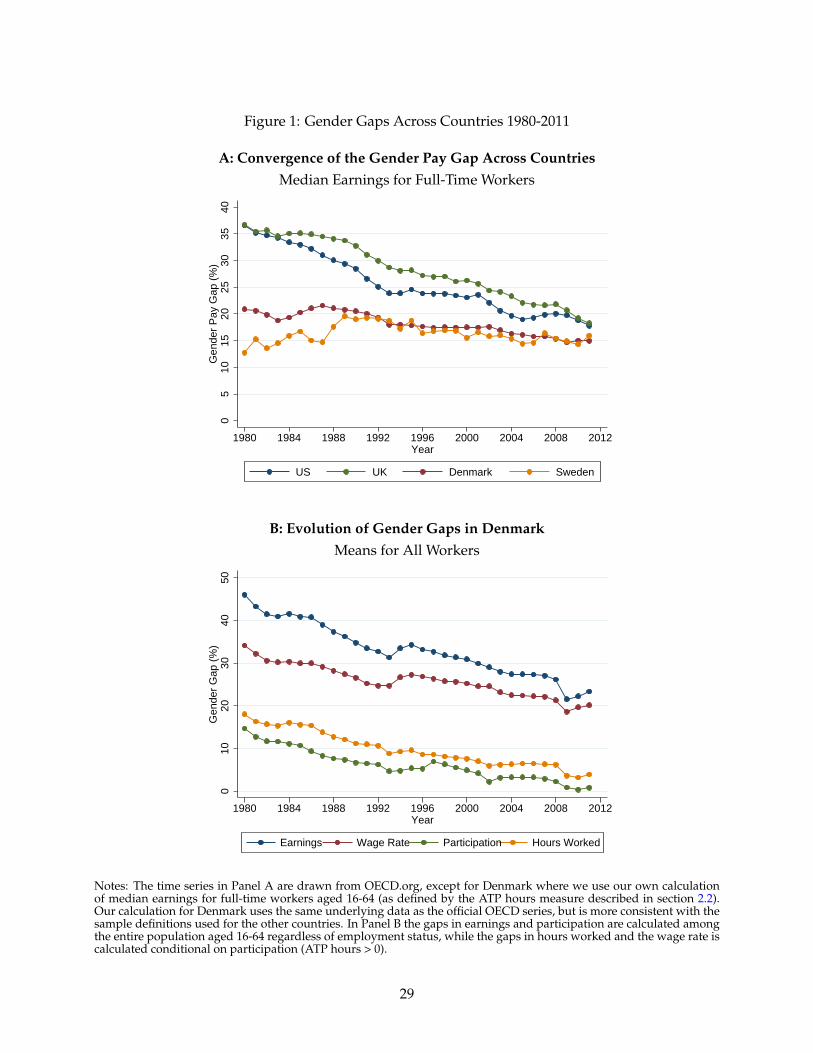
Figure 1: Gender Gaps Across Countries 1980-2011

A: Convergence of the Gender Pay Gap Across CountriesMedian Earnings for Full-Time Workers

05

1015

2025

3035

40G

ende

r P

ay G

ap (

%)

1980 1984 1988 1992 1996 2000 2004 2008 2012Year

US UK Denmark Sweden

B: Evolution of Gender Gaps in DenmarkMeans for All Workers

010

2030

4050

Gen

der

Gap

(%

)

1980 1984 1988 1992 1996 2000 2004 2008 2012Year

Earnings Wage Rate Participation Hours Worked

Notes: The time series in Panel A are drawn from OECD.org, except for Denmark where we use our own calculationof median earnings for full-time workers aged 16-64 (as defined by the ATP hours measure described in section 2.2).Our calculation for Denmark uses the same underlying data as the official OECD series, but is more consistent with thesample definitions used for the other countries. In Panel B the gaps in earnings and participation are calculated amongthe entire population aged 16-64 regardless of employment status, while the gaps in hours worked and the wage rate iscalculated conditional on participation (ATP hours > 0).

29

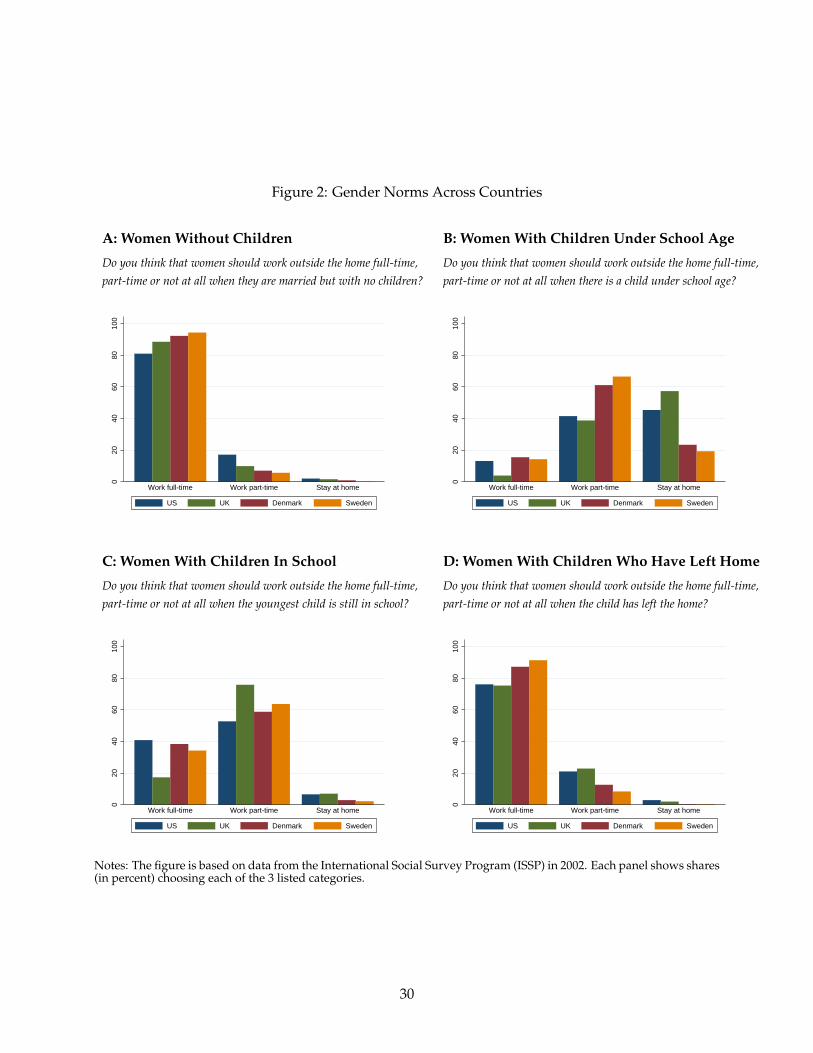
Figure 2: Gender Norms Across Countries

A: Women Without Children B: Women With Children Under School Age

Do you think that women should work outside the home full-time, Do you think that women should work outside the home full-time,part-time or not at all when they are married but with no children? part-time or not at all when there is a child under school age?

020

4060

8010

0

Work full-time Work part-time Stay at home

US UK Denmark Sweden

020

4060

8010

0

Work full-time Work part-time Stay at home

US UK Denmark Sweden

C: Women With Children In School D: Women With Children Who Have Left Home

Do you think that women should work outside the home full-time, Do you think that women should work outside the home full-time,part-time or not at all when the youngest child is still in school? part-time or not at all when the child has left the home?

020

4060

8010

0

Work full-time Work part-time Stay at home

US UK Denmark Sweden

020

4060

8010

0

Work full-time Work part-time Stay at home

US UK Denmark Sweden

Notes: The figure is based on data from the International Social Survey Program (ISSP) in 2002. Each panel shows shares(in percent) choosing each of the 3 listed categories.

30

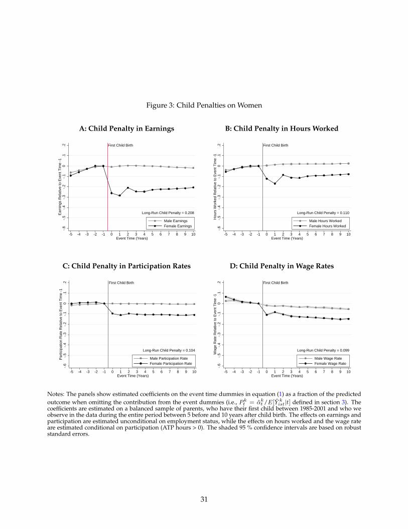
Figure 3: Child Penalties on Women

A: Child Penalty in Earnings B: Child Penalty in Hours Worked

First Child Birth

Long-Run Child Penalty = 0.208

-.6

-.5

-.4

-.3

-.2

-.1

0.1

.2E

arni

ngs

Rel

ativ

e to

Eve

nt T

ime

-1

-5 -4 -3 -2 -1 0 1 2 3 4 5 6 7 8 9 10Event Time (Years)

Male EarningsFemale Earnings

First Child Birth

Long-Run Child Penalty = 0.110

-.6

-.5

-.4

-.3

-.2

-.1

0.1

.2H

ours

Wor

ked

Rel

ativ

e to

Eve

nt T

ime

-1

-5 -4 -3 -2 -1 0 1 2 3 4 5 6 7 8 9 10Event Time (Years)

Male Hours WorkedFemale Hours Worked

C: Child Penalty in Participation Rates D: Child Penalty in Wage Rates

First Child Birth

Long-Run Child Penalty = 0.104

-.6

-.5

-.4

-.3

-.2

-.1

0.1

.2P

artic

ipat

ion

Rat

e R

elat

ive

to E

vent

Tim

e -1

-5 -4 -3 -2 -1 0 1 2 3 4 5 6 7 8 9 10Event Time (Years)

Male Participation RateFemale Participation Rate

First Child Birth

Long-Run Child Penalty = 0.099

-.6

-.5

-.4

-.3

-.2

-.1

0.1

.2W

age

Rat

e R

elat

ive

to E

vent

Tim

e -1

-5 -4 -3 -2 -1 0 1 2 3 4 5 6 7 8 9 10Event Time (Years)

Male Wage RateFemale Wage Rate

Notes: The panels show estimated coefficients on the event time dummies in equation (1) as a fraction of the predictedoutcome when omitting the contribution from the event dummies (i.e., P k

t = αkt /E[Y k

ist|t] defined in section 3). Thecoefficients are estimated on a balanced sample of parents, who have their first child between 1985-2001 and who weobserve in the data during the entire period between 5 before and 10 years after child birth. The effects on earnings andparticipation are estimated unconditional on employment status, while the effects on hours worked and the wage rateare estimated conditional on participation (ATP hours > 0). The shaded 95 % confidence intervals are based on robuststandard errors.

31

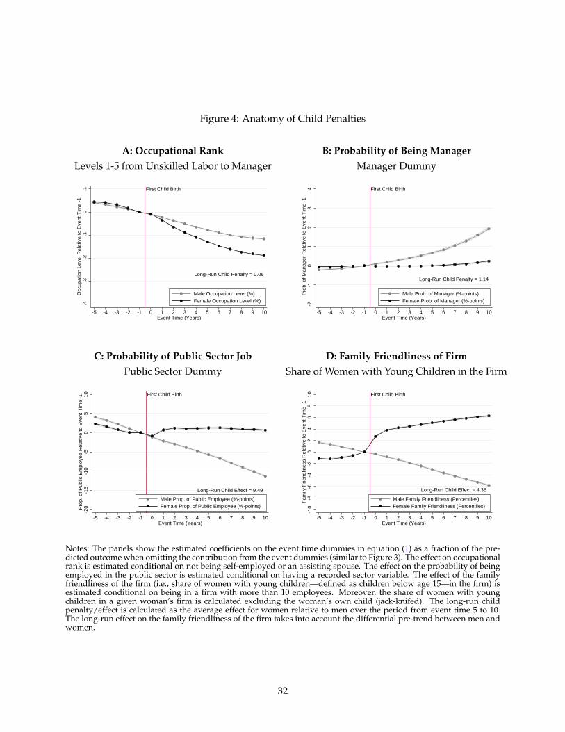
Figure 4: Anatomy of Child Penalties

A: Occupational Rank B: Probability of Being ManagerLevels 1-5 from Unskilled Labor to Manager Manager Dummy

First Child Birth

Long-Run Child Penalty = 0.06

-.4

-.3

-.2

-.1

0.1

Occ

upat

ion

Leve

l Rel

ativ

e to

Eve

nt T

ime

-1

-5 -4 -3 -2 -1 0 1 2 3 4 5 6 7 8 9 10Event Time (Years)

Male Occupation Level (%)Female Occupation Level (%)

First Child Birth

Long-Run Child Penalty = 1.14

-2-1

01

23

4P

rob.

of M

anag

er R

elat

ive

to E

vent

Tim

e -1

-5 -4 -3 -2 -1 0 1 2 3 4 5 6 7 8 9 10Event Time (Years)

Male Prob. of Manager (%-points)Female Prob. of Manager (%-points)

C: Probability of Public Sector Job D: Family Friendliness of FirmPublic Sector Dummy Share of Women with Young Children in the Firm

First Child Birth

Long-Run Child Effect = 9.49

-20

-15

-10

-50

510

Pro

p. o

f Pub

lic E

mpl

oyee

Rel

ativ

e to

Eve

nt T

ime

-1

-5 -4 -3 -2 -1 0 1 2 3 4 5 6 7 8 9 10Event Time (Years)

Male Prop. of Public Employee (%-points)Female Prop. of Public Employee (%-points)

First Child Birth

Long-Run Child Effect = 4.36

-10

-8-6

-4-2

02

46

810

Fam

ily F

riend

lines

s R

elat

ive

to E

vent

Tim

e -1

-5 -4 -3 -2 -1 0 1 2 3 4 5 6 7 8 9 10Event Time (Years)

Male Family Friendliness (Percentiles)Female Family Friendliness (Percentiles)

Notes: The panels show the estimated coefficients on the event time dummies in equation (1) as a fraction of the pre-dicted outcome when omitting the contribution from the event dummies (similar to Figure 3). The effect on occupationalrank is estimated conditional on not being self-employed or an assisting spouse. The effect on the probability of beingemployed in the public sector is estimated conditional on having a recorded sector variable. The effect of the familyfriendliness of the firm (i.e., share of women with young children—defined as children below age 15—in the firm) isestimated conditional on being in a firm with more than 10 employees. Moreover, the share of women with youngchildren in a given woman’s firm is calculated excluding the woman’s own child (jack-knifed). The long-run childpenalty/effect is calculated as the average effect for women relative to men over the period from event time 5 to 10.The long-run effect on the family friendliness of the firm takes into account the differential pre-trend between men andwomen.

32

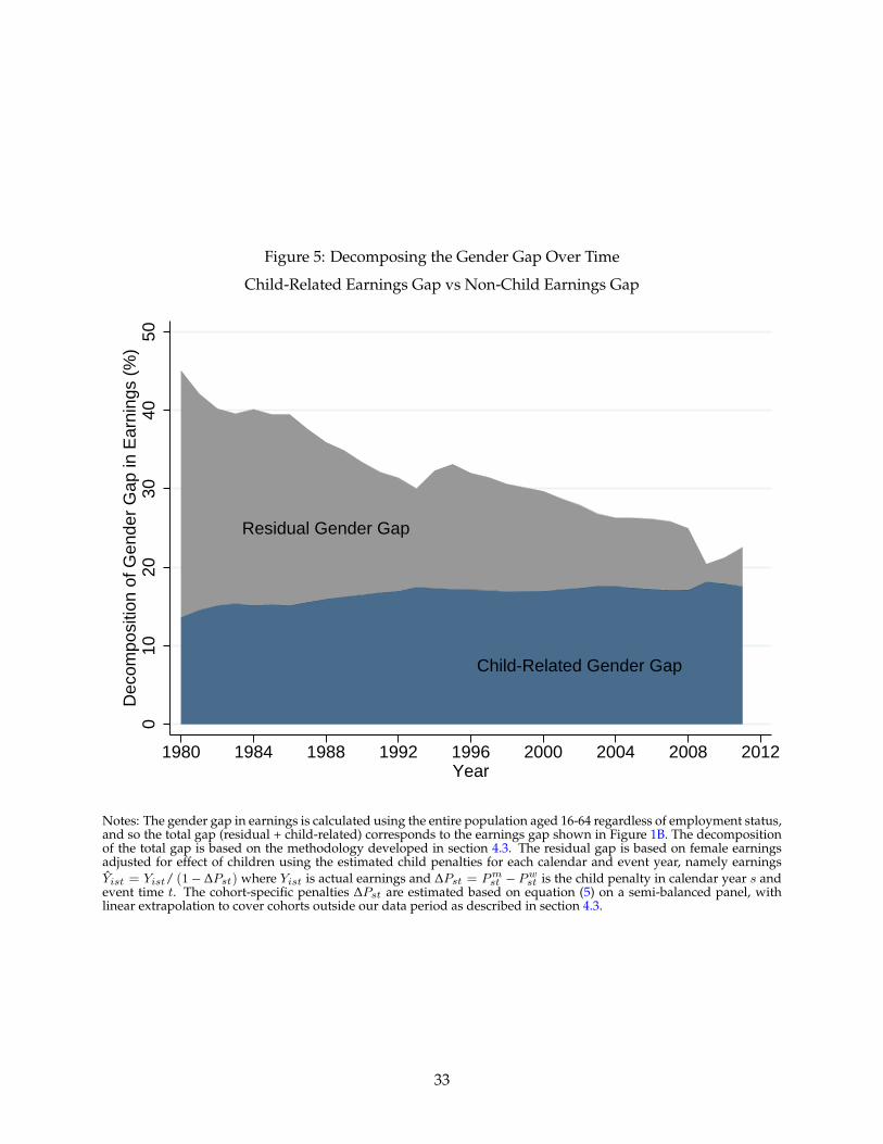
Figure 5: Decomposing the Gender Gap Over Time

Child-Related Earnings Gap vs Non-Child Earnings Gap

Residual Gender Gap

Child-Related Gender Gap

010

2030

4050

Dec

ompo

sitio

n of

Gen

der

Gap

in E

arni

ngs

(%)

1980 1984 1988 1992 1996 2000 2004 2008 2012Year

Notes: The gender gap in earnings is calculated using the entire population aged 16-64 regardless of employment status,and so the total gap (residual + child-related) corresponds to the earnings gap shown in Figure 1B. The decompositionof the total gap is based on the methodology developed in section 4.3. The residual gap is based on female earningsadjusted for effect of children using the estimated child penalties for each calendar and event year, namely earningsYist = Yist/ (1− ∆Pst) where Yist is actual earnings and ∆Pst = Pm

st − Pwst is the child penalty in calendar year s and

event time t. The cohort-specific penalties ∆Pst are estimated based on equation (5) on a semi-balanced panel, withlinear extrapolation to cover cohorts outside our data period as described in section 4.3.

33

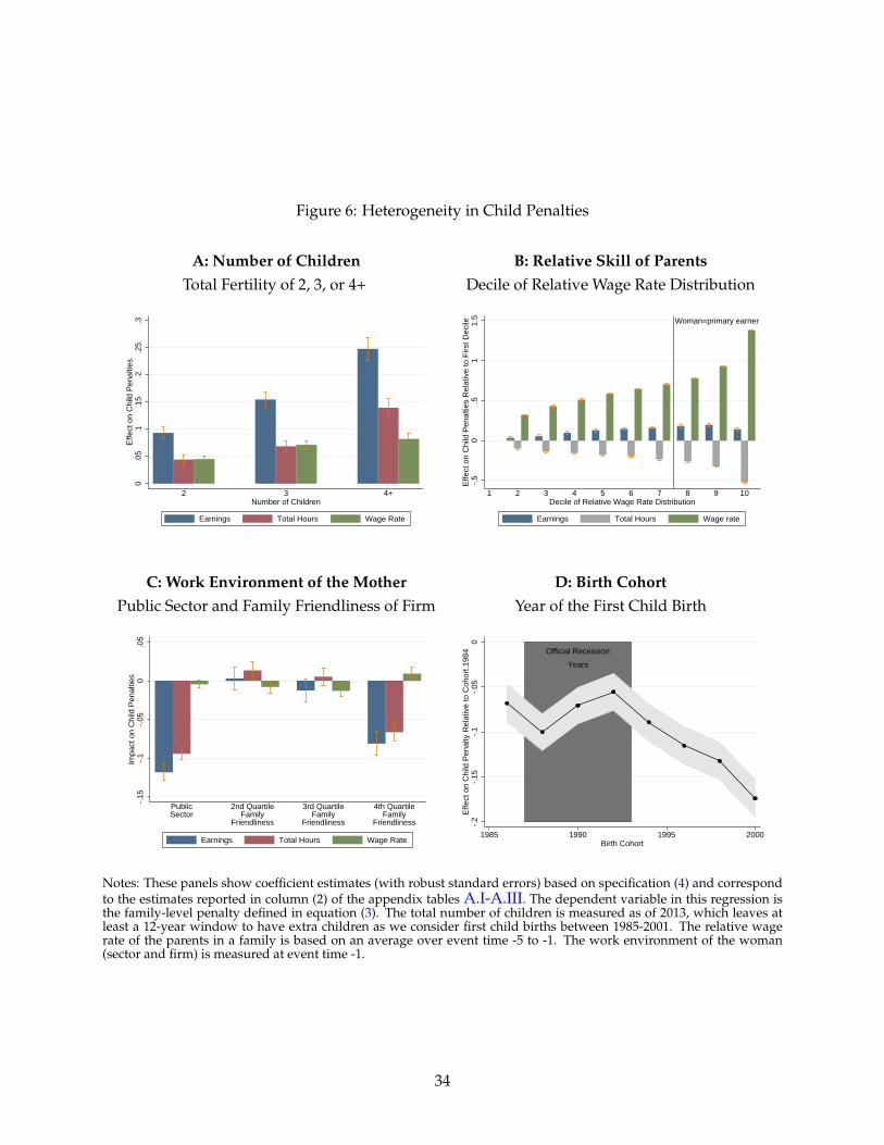
Figure 6: Heterogeneity in Child Penalties

A: Number of Children B: Relative Skill of ParentsTotal Fertility of 2, 3, or 4+ Decile of Relative Wage Rate Distribution

0.0

5.1

.15

.2.2

5.3

Effe

ct o

n C

hild

Pen

altie

s

2 3 4+Number of Children

Earnings Total Hours Wage Rate

Woman=primary earner

-.5

0.5

11.

5E

ffect

on

Chi

ld P

enal

ties

Rel

ativ

e to

Firs

t Dec

ile

1 2 3 4 5 6 7 8 9 10Decile of Relative Wage Rate Distribution

Earnings Total Hours Wage rate

C: Work Environment of the Mother D: Birth CohortPublic Sector and Family Friendliness of Firm Year of the First Child Birth

-.15

-.1

-.05

0.0

5Im

pact

on

Chi

ld P

enal

ties

PublicSector

2nd QuartileFamily

Friendliness

3rd QuartileFamily

Friendliness

4th QuartileFamily

Friendliness

Earnings Total Hours Wage Rate

Official Recession

Years

-.2

-.15

-.1

-.05

0E

ffect

on

Chi

ld P

enal

ty R

elat

ive

to C

ohor

t 198

4

1985 1990 1995 2000Birth Cohort

Notes: These panels show coefficient estimates (with robust standard errors) based on specification (4) and correspondto the estimates reported in column (2) of the appendix tables A.I-A.III. The dependent variable in this regression isthe family-level penalty defined in equation (3). The total number of children is measured as of 2013, which leaves atleast a 12-year window to have extra children as we consider first child births between 1985-2001. The relative wagerate of the parents in a family is based on an average over event time -5 to -1. The work environment of the woman(sector and firm) is measured at event time -1.

34

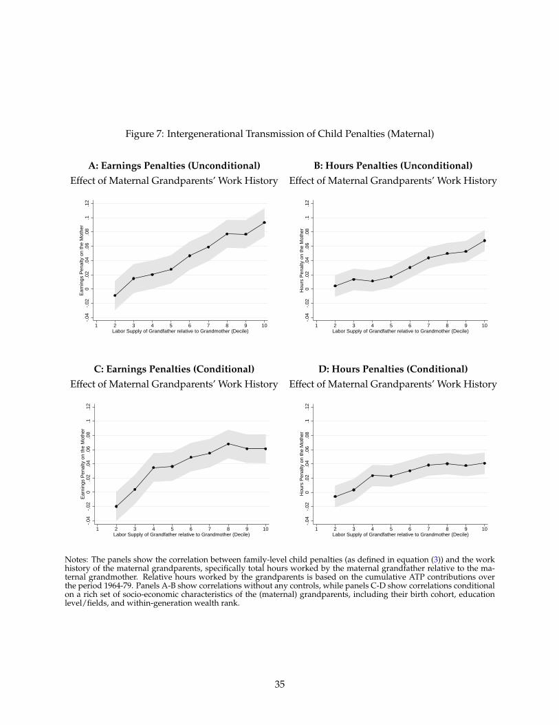
Figure 7: Intergenerational Transmission of Child Penalties (Maternal)

A: Earnings Penalties (Unconditional) B: Hours Penalties (Unconditional)Effect of Maternal Grandparents’ Work History Effect of Maternal Grandparents’ Work History

-.04

-.02

0.0

2.0

4.0

6.0

8.1

.12

Ear

ning

s P

enal

ty o

n th

e M

othe

r

1 2 3 4 5 6 7 8 9 10Labor Supply of Grandfather relative to Grandmother (Decile)

-.04

-.02

0.0

2.0

4.0

6.0

8.1

.12

Hou

rs P

enal

ty o

n th

e M

othe

r

1 2 3 4 5 6 7 8 9 10Labor Supply of Grandfather relative to Grandmother (Decile)

C: Earnings Penalties (Conditional) D: Hours Penalties (Conditional)Effect of Maternal Grandparents’ Work History Effect of Maternal Grandparents’ Work History

-.04

-.02

0.0

2.0

4.0

6.0

8.1

.12

Ear

ning

s P

enal

ty o

n th

e M

othe

r

1 2 3 4 5 6 7 8 9 10Labor Supply of Grandfather relative to Grandmother (Decile)

-.04

-.02

0.0

2.0

4.0

6.0

8.1

.12

Hou

rs P

enal

ty o

n th

e M

othe

r

1 2 3 4 5 6 7 8 9 10Labor Supply of Grandfather relative to Grandmother (Decile)

Notes: The panels show the correlation between family-level child penalties (as defined in equation (3)) and the workhistory of the maternal grandparents, specifically total hours worked by the maternal grandfather relative to the ma-ternal grandmother. Relative hours worked by the grandparents is based on the cumulative ATP contributions overthe period 1964-79. Panels A-B show correlations without any controls, while panels C-D show correlations conditionalon a rich set of socio-economic characteristics of the (maternal) grandparents, including their birth cohort, educationlevel/fields, and within-generation wealth rank.

35

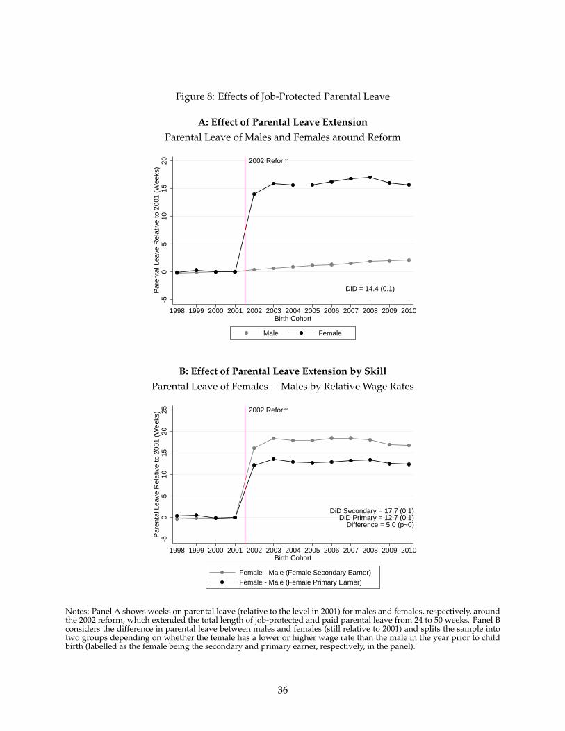
Figure 8: Effects of Job-Protected Parental Leave

A: Effect of Parental Leave ExtensionParental Leave of Males and Females around Reform

2002 Reform

DiD = 14.4 (0.1)

-50

510

1520

Par

enta

l Lea

ve R

elat

ive

to 2

001

(Wee

ks)

1998 1999 2000 2001 2002 2003 2004 2005 2006 2007 2008 2009 2010Birth Cohort

Male Female

B: Effect of Parental Leave Extension by SkillParental Leave of Females −Males by Relative Wage Rates

2002 Reform

DiD Secondary = 17.7 (0.1)DiD Primary = 12.7 (0.1)

Difference = 5.0 (p~0)

-50

510

1520

25P

aren

tal L

eave

Rel

ativ

e to

200

1 (W

eeks

)

1998 1999 2000 2001 2002 2003 2004 2005 2006 2007 2008 2009 2010Birth Cohort

Female - Male (Female Secondary Earner)Female - Male (Female Primary Earner)

Notes: Panel A shows weeks on parental leave (relative to the level in 2001) for males and females, respectively, aroundthe 2002 reform, which extended the total length of job-protected and paid parental leave from 24 to 50 weeks. Panel Bconsiders the difference in parental leave between males and females (still relative to 2001) and splits the sample intotwo groups depending on whether the female has a lower or higher wage rate than the male in the year prior to childbirth (labelled as the female being the secondary and primary earner, respectively, in the panel).

36

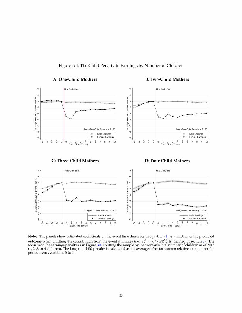
Figure A.I: The Child Penalty in Earnings by Number of Children

A: One-Child Mothers B: Two-Child Mothers

First Child Birth

Long-Run Child Penalty = 0.103

-.6

-.5

-.4

-.3

-.2

-.1

0.1

.2E

arni

ngs

Rel

ativ

e to

Eve

nt T

ime

-1

-5 -4 -3 -2 -1 0 1 2 3 4 5 6 7 8 9 10Event Time (Years)

Male EarningsFemale Earnings

First Child Birth

Long-Run Child Penalty = 0.196-.

6-.

5-.

4-.

3-.

2-.

10

.1.2

Ear

ning

s R

elat

ive

to E

vent

Tim

e -1

-5 -4 -3 -2 -1 0 1 2 3 4 5 6 7 8 9 10Event Time (Years)

Male EarningsFemale Earnings

C: Three-Child Mothers D: Four-Child Mothers

First Child Birth

Long-Run Child Penalty = 0.282

-.6

-.5

-.4

-.3

-.2

-.1

0.1

.2E

arni

ngs

Rel

ativ

e to

Eve

nt T

ime

-1

-5 -4 -3 -2 -1 0 1 2 3 4 5 6 7 8 9 10Event Time (Years)

Male EarningsFemale Earnings

First Child Birth

Long-Run Child Penalty = 0.380

-.6

-.5

-.4

-.3

-.2

-.1

0.1

.2E

arni

ngs

Rel

ativ

e to

Eve

nt T

ime

-1

-5 -4 -3 -2 -1 0 1 2 3 4 5 6 7 8 9 10Event Time (Years)

Male EarningsFemale Earnings

Notes: The panels show estimated coefficients on the event time dummies in equation (1) as a fraction of the predictedoutcome when omitting the contribution from the event dummies (i.e., P k

t = αkt /E[Y k

ist|t] defined in section 3). Thefocus is on the earnings penalty as in Figure 3A, splitting the sample by the woman’s total number of children as of 2013(1, 2, 3, or 4 children). The long-run child penalty is calculated as the average effect for women relative to men over theperiod from event time 5 to 10.

37

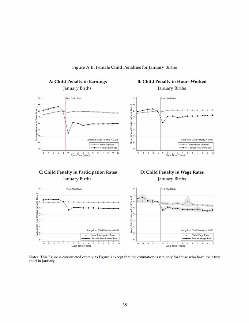
Figure A.II: Female Child Penalties for January Births

A: Child Penalty in Earnings B: Child Penalty in Hours WorkedJanuary Births January Births

First Child Birth

Long-Run Child Penalty = 0.178

-.6

-.5

-.4

-.3

-.2

-.1

0.1

.2E

arni

ngs

Rel

ativ

e to

Eve

nt T

ime

-1

-5 -4 -3 -2 -1 0 1 2 3 4 5 6 7 8 9 10Event Time (Years)

Male EarningsFemale Earnings

First Child Birth

Long-Run Child Penalty = 0.089

-.6

-.5

-.4

-.3

-.2

-.1

0.1

.2H

ours

Wor

ked

Rel

ativ

e to

Eve

nt T

ime

-1

-5 -4 -3 -2 -1 0 1 2 3 4 5 6 7 8 9 10Event Time (Years)

Male Hours WorkedFemale Hours Worked

C: Child Penalty in Participation Rates D: Child Penalty in Wage RatesJanuary Births January Births

First Child Birth

Long-Run Child Penalty = 0.095

-.6

-.5

-.4

-.3

-.2

-.1

0.1

.2P

artic

ipat

ion

Rat

e R

elat

ive

to E

vent

Tim

e -1

-5 -4 -3 -2 -1 0 1 2 3 4 5 6 7 8 9 10Event Time (Years)

Male Participation RateFemale Participation Rate

First Child Birth

Long-Run Child Penalty = 0.085

-.6

-.5

-.4

-.3

-.2

-.1

0.1

.2W

age

Rat

e R

elat

ive

to E

vent

Tim

e -1

-5 -4 -3 -2 -1 0 1 2 3 4 5 6 7 8 9 10Event Time (Years)

Male Wage RateFemale Wage Rate

Notes: This figure is constructed exactly as Figure 3 except that the estimation is run only for those who have their firstchild in January.

38

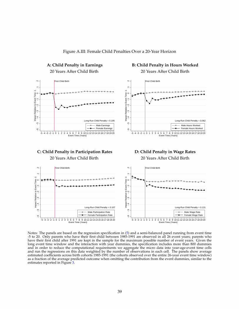
Figure A.III: Female Child Penalties Over a 20-Year Horizon

A: Child Penalty in Earnings B: Child Penalty in Hours Worked20 Years After Child Birth 20 Years After Child Birth

First Child Birth

Long-Run Child Penalty = 0.195

-.6

-.5

-.4

-.3

-.2

-.1

0.1

.2Im

pact

Rel

ativ

e to

Eve

nt T

ime

-1

-5 -4 -3 -2 -1 0 1 2 3 4 5 6 7 8 9 10 11 12 13 14 15 16 17 18 19 20Event Time (Years)

Male EarningsFemale Earnings

First Child Birth

Long-Run Child Penalty = 0.062

-.6

-.5

-.4

-.3

-.2

-.1

0.1

.2Im

pact

Rel

ativ

e to

Eve

nt T

ime

-1

-5 -4 -3 -2 -1 0 1 2 3 4 5 6 7 8 9 10 11 12 13 14 15 16 17 18 19 20Event Time (Years)

Male Hours WorkedFemale Hours Worked

C: Child Penalty in Participation Rates D: Child Penalty in Wage Rates20 Years After Child Birth 20 Years After Child Birth

First Child Birth

Long-Run Child Penalty = 0.107

-.6

-.5

-.4

-.3

-.2

-.1

0.1

.2Im

pact

Rel

ativ

e to

Eve

nt T

ime

-1

-5 -4 -3 -2 -1 0 1 2 3 4 5 6 7 8 9 10 11 12 13 14 15 16 17 18 19 20Event Time (Years)

Male Participation RateFemale Participation Rate

First Child Birth

Long-Run Child Penalty = 0.131

-.6

-.5

-.4

-.3

-.2

-.1

0.1

.2Im

pact

Rel

ativ

e to

Eve

nt T

ime

-1

-5 -4 -3 -2 -1 0 1 2 3 4 5 6 7 8 9 10 11 12 13 14 15 16 17 18 19 20Event Time (Years)

Male Wage RateFemale Wage Rate

Notes: The panels are based on the regression specification in (5) and a semi-balanced panel running from event time-5 to 20. Only parents who have their first child between 1985-1991 are observed in all 26 event years; parents whohave their first child after 1991 are kept in the sample for the maximum possible number of event years. Given thelong event time window and the interaction with year dummies, the specification includes more than 800 dummiesand in order to reduce the computational requirements we aggregate the micro data into year-age-event time cellsand run the regressions on this data weighted by the number of observations in each cell. The panels show averageestimated coefficients across birth cohorts 1985-1991 (the cohorts observed over the entire 26-year event time window)as a fraction of the average predicted outcome when omitting the contribution from the event dummies, similar to theestimates reported in Figure 3.

39

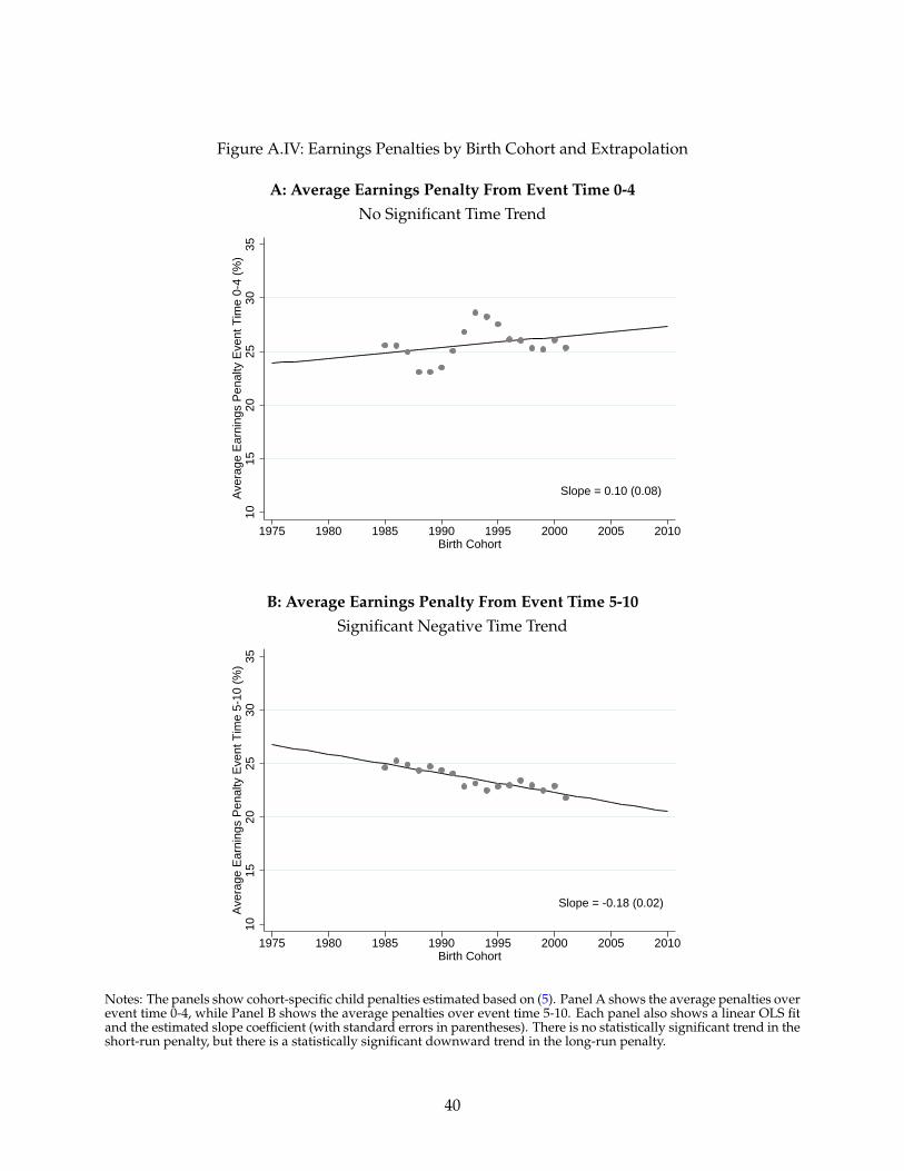
Figure A.IV: Earnings Penalties by Birth Cohort and Extrapolation

A: Average Earnings Penalty From Event Time 0-4No Significant Time Trend

Slope = 0.10 (0.08)

1015

2025

3035

Ave

rage

Ear

ning

s P

enal

ty E

vent

Tim

e 0-

4 (%

)

1975 1980 1985 1990 1995 2000 2005 2010Birth Cohort

B: Average Earnings Penalty From Event Time 5-10Significant Negative Time Trend

Slope = -0.18 (0.02)

1015

2025

3035

Ave

rage

Ear

ning

s P

enal

ty E

vent

Tim

e 5-

10 (

%)

1975 1980 1985 1990 1995 2000 2005 2010Birth Cohort

Notes: The panels show cohort-specific child penalties estimated based on (5). Panel A shows the average penalties overevent time 0-4, while Panel B shows the average penalties over event time 5-10. Each panel also shows a linear OLS fitand the estimated slope coefficient (with standard errors in parentheses). There is no statistically significant trend in theshort-run penalty, but there is a statistically significant downward trend in the long-run penalty.

40

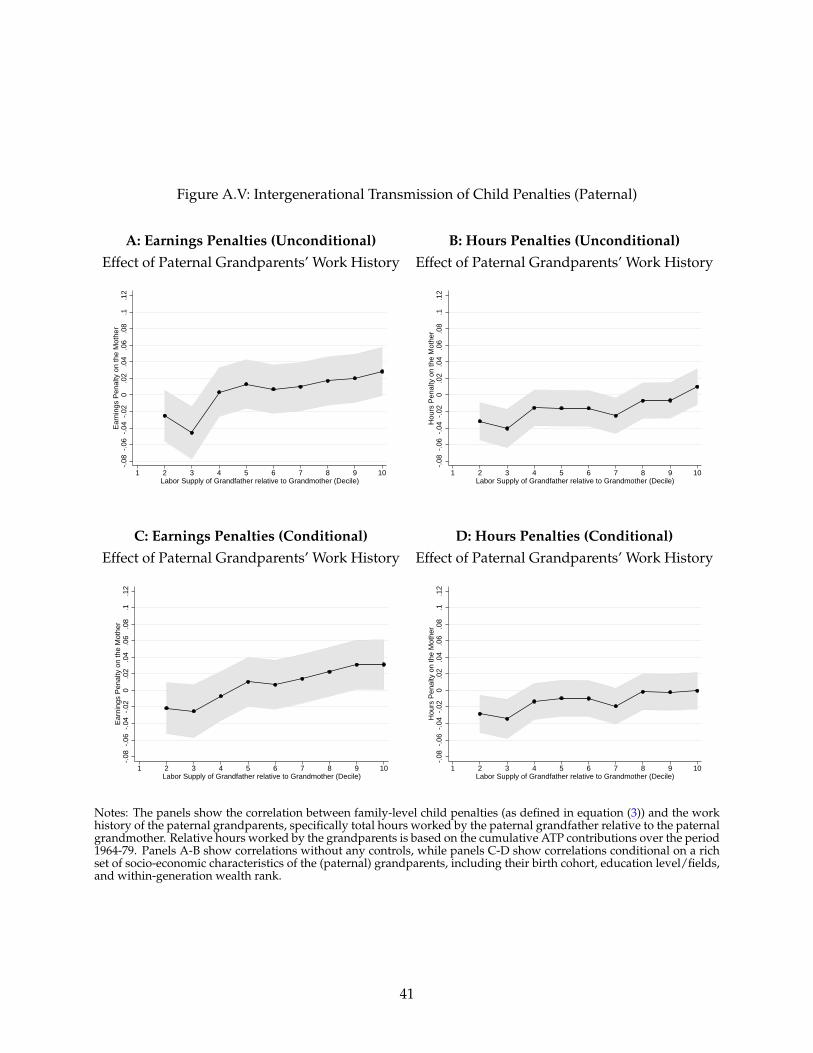
Figure A.V: Intergenerational Transmission of Child Penalties (Paternal)

A: Earnings Penalties (Unconditional) B: Hours Penalties (Unconditional)Effect of Paternal Grandparents’ Work History Effect of Paternal Grandparents’ Work History

-.08

-.06

-.04

-.02

0.0

2.0

4.0

6.0

8.1

.12

Ear

ning

s P

enal

ty o

n th

e M

othe

r

1 2 3 4 5 6 7 8 9 10Labor Supply of Grandfather relative to Grandmother (Decile)

-.08

-.06

-.04

-.02

0.0

2.0

4.0

6.0

8.1

.12

Hou

rs P

enal

ty o

n th

e M

othe

r

1 2 3 4 5 6 7 8 9 10Labor Supply of Grandfather relative to Grandmother (Decile)

C: Earnings Penalties (Conditional) D: Hours Penalties (Conditional)Effect of Paternal Grandparents’ Work History Effect of Paternal Grandparents’ Work History

-.08

-.06

-.04

-.02

0.0

2.0

4.0

6.0

8.1

.12

Ear

ning

s P

enal

ty o

n th

e M

othe

r

1 2 3 4 5 6 7 8 9 10Labor Supply of Grandfather relative to Grandmother (Decile)

-.08

-.06

-.04

-.02

0.0

2.0

4.0

6.0

8.1

.12

Hou

rs P

enal

ty o

n th

e M

othe

r

1 2 3 4 5 6 7 8 9 10Labor Supply of Grandfather relative to Grandmother (Decile)

Notes: The panels show the correlation between family-level child penalties (as defined in equation (3)) and the workhistory of the paternal grandparents, specifically total hours worked by the paternal grandfather relative to the paternalgrandmother. Relative hours worked by the grandparents is based on the cumulative ATP contributions over the period1964-79. Panels A-B show correlations without any controls, while panels C-D show correlations conditional on a richset of socio-economic characteristics of the (paternal) grandparents, including their birth cohort, education level/fields,and within-generation wealth rank.

41

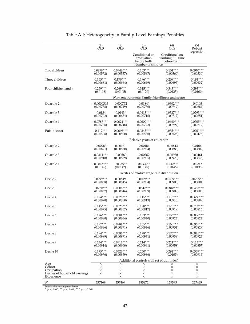
Table A.I: Heterogeneity in Family-Level Earnings Penalties

(1) (2) (3) (4) (5)OLS OLS OLS OLS Robust

regressionConditional on Conditional on

graduation working full timebefore birth before birthNumber of children

Two children 0.0898∗∗∗ 0.0946∗∗∗ 0.103∗∗∗ 0.104∗∗∗ 0.0970∗∗∗(0.00572) (0.00557) (0.00567) (0.00560) (0.00530)

Three children 0.155∗∗∗ 0.170∗∗∗ 0.196∗∗∗ 0.209∗∗∗ 0.181∗∗∗(0.00681) (0.00664) (0.00699) (0.00695) (0.00632)

Four children and + 0.259∗∗∗ 0.269∗∗∗ 0.315∗∗∗ 0.343∗∗∗ 0.293∗∗∗(0.0108) (0.0105) (0.0120) (0.0125) (0.0100)

Work environment: Family friendliness and sector

Quartile 2 -0.0000305 -0.000772 -0.0184∗ -0.0302∗∗∗ -0.0105(0.00738) (0.00719) (0.00750) (0.00749) (0.00684)

Quartile 3 -0.0134 -0.0143∗ -0.0413∗∗∗ -0.0527∗∗∗ -0.0293∗∗∗(0.00702) (0.00684) (0.00716) (0.00717) (0.00651)

Quartile 4 -0.0787∗∗∗ -0.0624∗∗∗ -0.0600∗∗∗ -0.0660∗∗∗ -0.0705∗∗∗(0.00768) (0.00748) (0.00792) (0.00797) (0.00712)

Public sector -0.112∗∗∗ -0.0649∗∗∗ -0.0345∗∗∗ -0.0354∗∗∗ -0.0701∗∗∗(0.00508) (0.00500) (0.00530) (0.00528) (0.00476)

Relative years of education

Quartile 2 -0.00963 0.00961 -0.00164 -0.00813 0.0106(0.00871) (0.00850) (0.00904) (0.00888) (0.00809)

Quartile 3 -0.0314∗∗∗ -0.00560 -0.00762 -0.00930 0.00461(0.00910) (0.00889) (0.00935) (0.00920) (0.00846)

Quartile 4 -0.0815∗∗∗ -0.0375∗∗ -0.0396∗∗ -0.0425∗∗ -0.0242(0.0146) (0.0142) (0.0149) (0.0146) (0.0135)

Deciles of relative wage rate distribution

Decile 2 0.0299∗∗∗ 0.00849 0.0409∗∗∗ 0.0439∗∗∗ 0.0225∗∗(0.00868) (0.00845) (0.00904) (0.00905) (0.00804)

Decile 3 0.0770∗∗∗ 0.0306∗∗∗ 0.0842∗∗∗ 0.0848∗∗∗ 0.0453∗∗∗(0.00867) (0.00846) (0.00909) (0.00909) (0.00805)

Decile 4 0.124∗∗∗ 0.0528∗∗∗ 0.115∗∗∗ 0.116∗∗∗ 0.0668∗∗∗(0.00870) (0.00850) (0.00913) (0.00913) (0.00809)

Decile 5 0.145∗∗∗ 0.0525∗∗∗ 0.128∗∗∗ 0.125∗∗∗ 0.0702∗∗∗(0.00875) (0.00857) (0.00917) (0.00919) (0.00816)

Decile 6 0.176∗∗∗ 0.0681∗∗∗ 0.153∗∗∗ 0.153∗∗∗ 0.0836∗∗∗(0.00880) (0.00864) (0.00920) (0.00923) (0.00822)

Decile 7 0.197∗∗∗ 0.0781∗∗∗ 0.165∗∗∗ 0.165∗∗∗ 0.0965∗∗∗(0.00886) (0.00871) (0.00926) (0.00931) (0.00829)

Decile 8 0.194∗∗∗ 0.0686∗∗∗ 0.178∗∗∗ 0.176∗∗∗ 0.0845∗∗∗(0.00989) (0.00971) (0.00931) (0.00939) (0.00924)

Decile 9 0.234∗∗∗ 0.0912∗∗∗ 0.214∗∗∗ 0.224∗∗∗ 0.113∗∗∗(0.00914) (0.00900) (0.00941) (0.00958) (0.00857)

Decile 10 0.175∗∗∗ 0.0326∗∗∗ 0.230∗∗∗ 0.291∗∗∗ 0.0569∗∗∗(0.00976) (0.00959) (0.00986) (0.0105) (0.00913)

Additional controls (full set of dummies)Age × × × × ×Cohort × × × × ×Occupation × × × × ×Deciles of household earnings × × × × ×Experience × × × ×

N 257469 257469 185872 159595 257469Standard errors in parentheses∗ p < 0.05, ∗∗ p < 0.01, ∗∗∗ p < 0.001

42

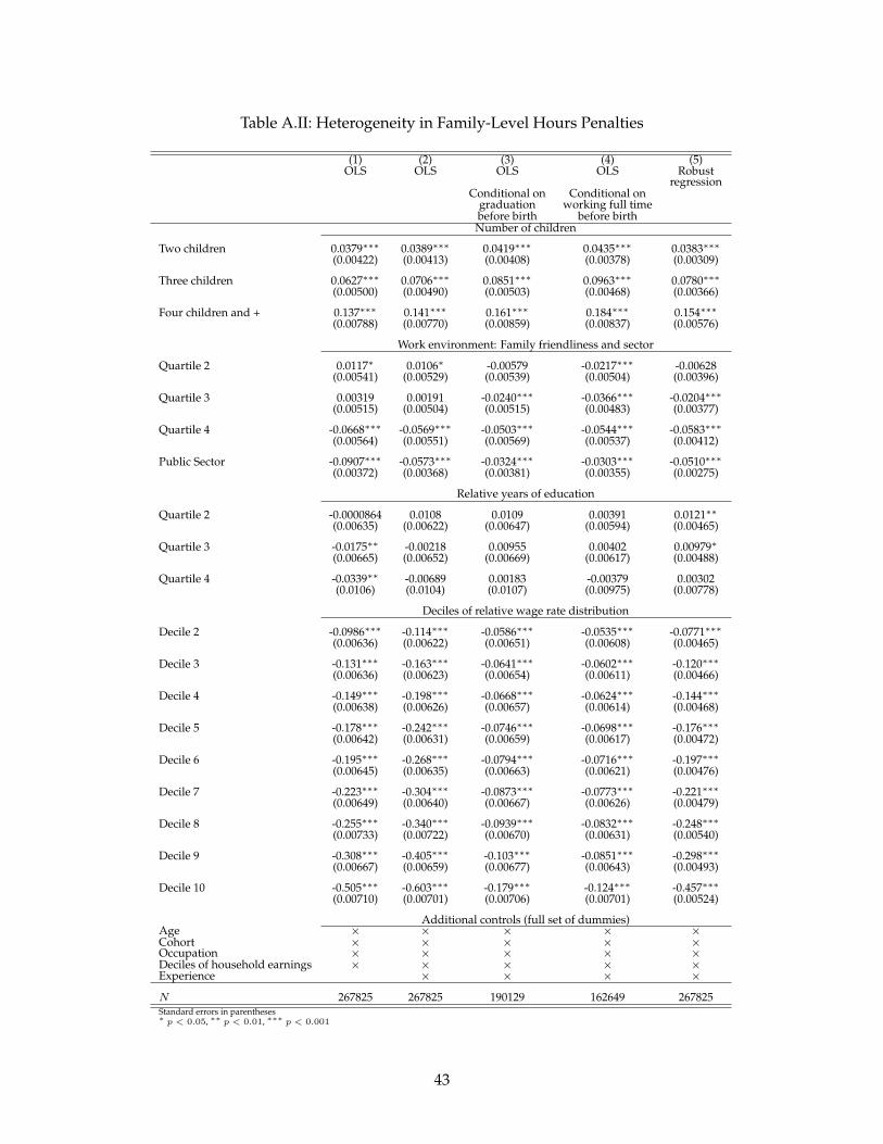
Table A.II: Heterogeneity in Family-Level Hours Penalties

(1) (2) (3) (4) (5)OLS OLS OLS OLS Robust

regressionConditional on Conditional on

graduation working full timebefore birth before birthNumber of children

Two children 0.0379∗∗∗ 0.0389∗∗∗ 0.0419∗∗∗ 0.0435∗∗∗ 0.0383∗∗∗(0.00422) (0.00413) (0.00408) (0.00378) (0.00309)

Three children 0.0627∗∗∗ 0.0706∗∗∗ 0.0851∗∗∗ 0.0963∗∗∗ 0.0780∗∗∗(0.00500) (0.00490) (0.00503) (0.00468) (0.00366)

Four children and + 0.137∗∗∗ 0.141∗∗∗ 0.161∗∗∗ 0.184∗∗∗ 0.154∗∗∗(0.00788) (0.00770) (0.00859) (0.00837) (0.00576)

Work environment: Family friendliness and sector

Quartile 2 0.0117∗ 0.0106∗ -0.00579 -0.0217∗∗∗ -0.00628(0.00541) (0.00529) (0.00539) (0.00504) (0.00396)

Quartile 3 0.00319 0.00191 -0.0240∗∗∗ -0.0366∗∗∗ -0.0204∗∗∗(0.00515) (0.00504) (0.00515) (0.00483) (0.00377)

Quartile 4 -0.0668∗∗∗ -0.0569∗∗∗ -0.0503∗∗∗ -0.0544∗∗∗ -0.0583∗∗∗(0.00564) (0.00551) (0.00569) (0.00537) (0.00412)

Public Sector -0.0907∗∗∗ -0.0573∗∗∗ -0.0324∗∗∗ -0.0303∗∗∗ -0.0510∗∗∗(0.00372) (0.00368) (0.00381) (0.00355) (0.00275)

Relative years of education

Quartile 2 -0.0000864 0.0108 0.0109 0.00391 0.0121∗∗(0.00635) (0.00622) (0.00647) (0.00594) (0.00465)

Quartile 3 -0.0175∗∗ -0.00218 0.00955 0.00402 0.00979∗(0.00665) (0.00652) (0.00669) (0.00617) (0.00488)

Quartile 4 -0.0339∗∗ -0.00689 0.00183 -0.00379 0.00302(0.0106) (0.0104) (0.0107) (0.00975) (0.00778)

Deciles of relative wage rate distribution

Decile 2 -0.0986∗∗∗ -0.114∗∗∗ -0.0586∗∗∗ -0.0535∗∗∗ -0.0771∗∗∗(0.00636) (0.00622) (0.00651) (0.00608) (0.00465)

Decile 3 -0.131∗∗∗ -0.163∗∗∗ -0.0641∗∗∗ -0.0602∗∗∗ -0.120∗∗∗(0.00636) (0.00623) (0.00654) (0.00611) (0.00466)

Decile 4 -0.149∗∗∗ -0.198∗∗∗ -0.0668∗∗∗ -0.0624∗∗∗ -0.144∗∗∗(0.00638) (0.00626) (0.00657) (0.00614) (0.00468)

Decile 5 -0.178∗∗∗ -0.242∗∗∗ -0.0746∗∗∗ -0.0698∗∗∗ -0.176∗∗∗(0.00642) (0.00631) (0.00659) (0.00617) (0.00472)

Decile 6 -0.195∗∗∗ -0.268∗∗∗ -0.0794∗∗∗ -0.0716∗∗∗ -0.197∗∗∗(0.00645) (0.00635) (0.00663) (0.00621) (0.00476)

Decile 7 -0.223∗∗∗ -0.304∗∗∗ -0.0873∗∗∗ -0.0773∗∗∗ -0.221∗∗∗(0.00649) (0.00640) (0.00667) (0.00626) (0.00479)

Decile 8 -0.255∗∗∗ -0.340∗∗∗ -0.0939∗∗∗ -0.0832∗∗∗ -0.248∗∗∗(0.00733) (0.00722) (0.00670) (0.00631) (0.00540)

Decile 9 -0.308∗∗∗ -0.405∗∗∗ -0.103∗∗∗ -0.0851∗∗∗ -0.298∗∗∗(0.00667) (0.00659) (0.00677) (0.00643) (0.00493)

Decile 10 -0.505∗∗∗ -0.603∗∗∗ -0.179∗∗∗ -0.124∗∗∗ -0.457∗∗∗(0.00710) (0.00701) (0.00706) (0.00701) (0.00524)

Additional controls (full set of dummies)Age × × × × ×Cohort × × × × ×Occupation × × × × ×Deciles of household earnings × × × × ×Experience × × × ×

N 267825 267825 190129 162649 267825Standard errors in parentheses∗ p < 0.05, ∗∗ p < 0.01, ∗∗∗ p < 0.001

43

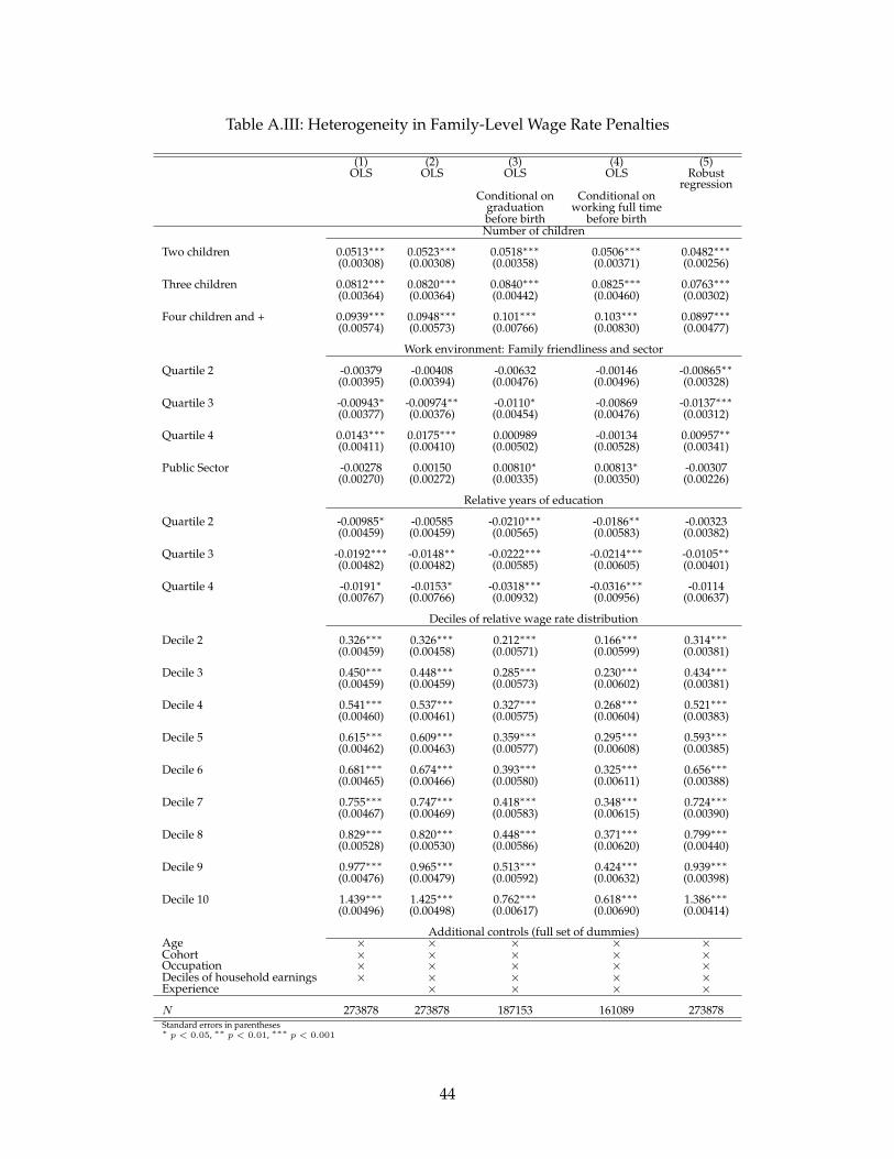
Table A.III: Heterogeneity in Family-Level Wage Rate Penalties

(1) (2) (3) (4) (5)OLS OLS OLS OLS Robust

regressionConditional on Conditional on

graduation working full timebefore birth before birthNumber of children

Two children 0.0513∗∗∗ 0.0523∗∗∗ 0.0518∗∗∗ 0.0506∗∗∗ 0.0482∗∗∗(0.00308) (0.00308) (0.00358) (0.00371) (0.00256)

Three children 0.0812∗∗∗ 0.0820∗∗∗ 0.0840∗∗∗ 0.0825∗∗∗ 0.0763∗∗∗(0.00364) (0.00364) (0.00442) (0.00460) (0.00302)

Four children and + 0.0939∗∗∗ 0.0948∗∗∗ 0.101∗∗∗ 0.103∗∗∗ 0.0897∗∗∗(0.00574) (0.00573) (0.00766) (0.00830) (0.00477)

Work environment: Family friendliness and sector

Quartile 2 -0.00379 -0.00408 -0.00632 -0.00146 -0.00865∗∗(0.00395) (0.00394) (0.00476) (0.00496) (0.00328)

Quartile 3 -0.00943∗ -0.00974∗∗ -0.0110∗ -0.00869 -0.0137∗∗∗(0.00377) (0.00376) (0.00454) (0.00476) (0.00312)

Quartile 4 0.0143∗∗∗ 0.0175∗∗∗ 0.000989 -0.00134 0.00957∗∗(0.00411) (0.00410) (0.00502) (0.00528) (0.00341)

Public Sector -0.00278 0.00150 0.00810∗ 0.00813∗ -0.00307(0.00270) (0.00272) (0.00335) (0.00350) (0.00226)

Relative years of education

Quartile 2 -0.00985∗ -0.00585 -0.0210∗∗∗ -0.0186∗∗ -0.00323(0.00459) (0.00459) (0.00565) (0.00583) (0.00382)

Quartile 3 -0.0192∗∗∗ -0.0148∗∗ -0.0222∗∗∗ -0.0214∗∗∗ -0.0105∗∗(0.00482) (0.00482) (0.00585) (0.00605) (0.00401)

Quartile 4 -0.0191∗ -0.0153∗ -0.0318∗∗∗ -0.0316∗∗∗ -0.0114(0.00767) (0.00766) (0.00932) (0.00956) (0.00637)

Deciles of relative wage rate distribution

Decile 2 0.326∗∗∗ 0.326∗∗∗ 0.212∗∗∗ 0.166∗∗∗ 0.314∗∗∗(0.00459) (0.00458) (0.00571) (0.00599) (0.00381)

Decile 3 0.450∗∗∗ 0.448∗∗∗ 0.285∗∗∗ 0.230∗∗∗ 0.434∗∗∗(0.00459) (0.00459) (0.00573) (0.00602) (0.00381)

Decile 4 0.541∗∗∗ 0.537∗∗∗ 0.327∗∗∗ 0.268∗∗∗ 0.521∗∗∗(0.00460) (0.00461) (0.00575) (0.00604) (0.00383)

Decile 5 0.615∗∗∗ 0.609∗∗∗ 0.359∗∗∗ 0.295∗∗∗ 0.593∗∗∗(0.00462) (0.00463) (0.00577) (0.00608) (0.00385)

Decile 6 0.681∗∗∗ 0.674∗∗∗ 0.393∗∗∗ 0.325∗∗∗ 0.656∗∗∗(0.00465) (0.00466) (0.00580) (0.00611) (0.00388)

Decile 7 0.755∗∗∗ 0.747∗∗∗ 0.418∗∗∗ 0.348∗∗∗ 0.724∗∗∗(0.00467) (0.00469) (0.00583) (0.00615) (0.00390)

Decile 8 0.829∗∗∗ 0.820∗∗∗ 0.448∗∗∗ 0.371∗∗∗ 0.799∗∗∗(0.00528) (0.00530) (0.00586) (0.00620) (0.00440)

Decile 9 0.977∗∗∗ 0.965∗∗∗ 0.513∗∗∗ 0.424∗∗∗ 0.939∗∗∗(0.00476) (0.00479) (0.00592) (0.00632) (0.00398)

Decile 10 1.439∗∗∗ 1.425∗∗∗ 0.762∗∗∗ 0.618∗∗∗ 1.386∗∗∗(0.00496) (0.00498) (0.00617) (0.00690) (0.00414)

Additional controls (full set of dummies)Age × × × × ×Cohort × × × × ×Occupation × × × × ×Deciles of household earnings × × × × ×Experience × × × ×

N 273878 273878 187153 161089 273878Standard errors in parentheses∗ p < 0.05, ∗∗ p < 0.01, ∗∗∗ p < 0.001

44