Child hunger in the developing world: An analysis of ...

Food Policy 30 (2005) 584–611

www.elsevier.com/locate/foodpol

Child hunger in the developing world: An analysisof environmental and social correlates

Deborah Balk a,*, Adam Storeygard a,1, Marc Levy a,1,Joanne Gaskell b,2, Manohar Sharma c,3, Rafael Flor d,4

a Center for International Earth Science Information Network, Columbia University, P.O. Box 1000, Palisades,

NY 10964, United Statesb Interdisciplinary Program in Environment and Resources, 397 Panama Mall, Mitchell Bldg Rm. 132,

Stanford University, Stanford, CA 94305-2210, United Statesc International Food Policy Research Institute, 2033 K Street NW, Washington, DC 20006-1002, United States

d Tropical Agriculture Program, Earth Institute at Columbia University, P.O. Box 1000, 61 Route 9W,

Lamont Hall 2E, Palisades, NY 10964, United States

Abstract

Using two complementary methods in a framework that allows incorporating both environmentaland household-level factors, we explore the correlates of underweight status among children. We useindividual children as the units of analysis in 19 African countries, and subnational survey strata in43 African, Asian and Latin American countries. We consider the relationship between household-level demographic and health survey data, environmental factors from external geospatial data setsand two indicators of malnutrition among children aged 1–3, deviations from the international stan-dards of weight-for-age and height-for-age. We discuss methods for data integration. In general,household determinants explain more variation than environmental factors, perhaps partly due tomore error-prone measurement at the community level. Among individual children, some measuresof agricultural capacity are related to lower incidence of child hunger, while among regions, mea-

0306-9192/$ - see front matter � 2005 Elsevier Ltd. All rights reserved.

doi:10.1016/j.foodpol.2005.10.007

* Corresponding author. Tel.: +1 845 365 8988; fax: +1 845 365 8922.E-mail addresses: [email protected] (D. Balk), [email protected] (A. Storeygard),

[email protected] (M. Levy), [email protected] (J. Gaskell), [email protected] (M. Sharma),[email protected] (R. Flor).1 Tel.: +1 845 365 8988; fax: +1 845 365 8922.2 Tel.: +1 650 725 5413.3 Tel.: +1 202 862 5600; fax: +1 202 467 4439.4 Tel.: +1 845 680 4531; fax: +1 845 680 4870.

mailto:[email protected]






D. Balk et al. / Food Policy 30 (2005) 584–611 585

sures relating to urbanness and population density show a stronger relationship. We give recommen-dations for further study, data collection and policy making.� 2005 Elsevier Ltd. All rights reserved.

Keywords: Child hunger; Underweight; Household; Environmental factors; Spatial analysis

Introduction

Despite the importance of understanding and reducing child hunger, the study of child-hood malnutrition has been limited to a degree by division into disciplinary approaches toanalysis. Social scientists have shown that individual and household-level factors such asbirth order or parental schooling are influential (cf. Charmarbagwala et al., 2004). Nutri-tionists have shown that there are hereditary and gender differences in the uptake of par-ticular nutrients and ultimately child nutritional outcomes (cf. Payne, 1990). Soil andclimate scientists have demonstrated the strong relationship between climate and soilpotential for agricultural sustainability and food production (Sanchez, 2002). While con-ceptual frameworks link these factors closely together (e.g., the UNICEF frameworkadapted from Smith and Haddad, 2000), few studies systematically assess them in combi-nation. Here, we attempt to close that gap.

Addressing environmental and socio-economic and demographic determinants of childhunger in an integrated fashion requires the adoption of a spatial framework of data inte-gration. Environmental data tend to be spatially referenced but not included in studies ofhousehold-level survey data. Thus, this analysis (1) converts spatial information into sur-vey units and (2) converts survey information into different spatial units. This method alsopresents us with an ability to improve the measurement of common, implicitly spatial fac-tors by treating them in explicitly spatial terms, for example, urban areas, disease vectorsand distances to important access points.

The United Nations Millennium Project Hunger Task Force (HTF) recently recom-mended complementary feeding along with continued breast-feeding until age 2 as oneof three pillars to reduce malnutrition in children aged under 5. Similarly, it recommendedreducing vulnerability through productive safety nets (e.g., local early warning systems),increasing income and access to markets for the poor (e.g., increase capacity of rural townsand market-related infrastructure, and increase non-farm-dependent income generation)and restoring and conserving essential natural resources for food security (Sanchezet al., 2005). This study allows for a preliminary analysis of how the current state of someof these factors affect child hunger.

Study design and data

Anthropometric indicators from household survey data have long been used as mea-sures of health and nutritional status (Tanner, 1981). Anthropometric indicators are rela-tively easy to determine for every child in large-scale representative surveys. The data canbe compared across countries, ‘‘There is evidence that the growth in height and weight of

586 D. Balk et al. / Food Policy 30 (2005) 584–611

well fed, healthy children, or children who experience unconstrained growth, from differ-ent ethnic backgrounds and different continents is reasonably similar, at least up to 5 yearsof age. While it is accepted that there are variations in the growth patterns of childrenfrom different racial or ethnic groups in developed countries, these are relatively minorcompared with the large worldwide variation that relates to health, nutrition, and socio-economic status’’ (WHO, 1995).5

Individual-level anthropometric data collected through surveys may also be combinedin analysis with all the other data found in those surveys. Several conceptual frameworkshave been proposed, placing causes of child malnutrition in a theoretical context (UNI-CEF, 1990, 1998, further adapted by Engle et al., 1999 and Smith and Haddad, 2000).The Smith and Haddad framework (p. 6), for example, encompasses socio-economicand biological factors operating at household, community and institutional levels. Inthe past, however, household surveys used for testing this framework have not contained(or been linked to) any information on many of its components.

In the past 15 years, Demographic and Health Surveys (DHS) conducted in over 30countries have begun to include information about the geographic location of surveyrespondents. This can then be coupled with factors that are geographically determinedor recorded, such as soil quality, agricultural production, population density and dis-tance to a port, to be analysed in combination with the survey data (cf. Balk et al.,2004). These variables are thought to exert influence over and above those effects whichare mediated by household characteristics (such as parental schooling or wealth) but inthe absence of a geospatial framework are generally explained as regional affects, or sim-ply unexplained variance. Thus, we consider the relationship between child malnutrition,as measured by weight-for-age and height-for-age Z scores (WHO, 1995), and selectedbiophysical and macro-demographic variables joined to the anthropometric data viageographic location.

We conducted the analysis in two phases, corresponding to two levels of analysis, bothof which have inherent strengths and weaknesses. Individual-level analysis permits a muchfuller examination of behavioural factors than could be considered at a subnational level.The number of observations is great (n = 33,000 children), allowing for practically unlim-ited permutations of variables in form or in combination with others (e.g., interactions).However, it is geographically limited to parts of Africa. Additionally, policy is generallytargeted at a level above the household, and while individual-level analyses may be a crit-ical piece of constructing policies, they may also fall short of understanding aspects of theproblem that can be best summarized at a regional scale.

The meso-scale analysis has greater geographic breadth and provides a valuable toolfor analysts designing policies for whole provinces. But it poses additional pitfalls. Thereare far fewer units in the analysis (n = 319 subnational units), so the risk of reducing thepower of the model by introducing too many variables (such as a full suite of interactionterms) is increased. Correspondingly, aggregation removes the variance within each sub-national region both among the variables native to the household survey, which must besummarized, and among the variables external to the survey, which must be recalculated

5 Several studies have concluded that there are no biological differences in ethnicity that might bias comparisonof children in a global analysis of weight-for-age status (Habicht et al., 1974; Graitcher and Gentry, 1981;Whitehead and Paul, 1984).


for the region as a whole. Thus, the ecological fallacy must be accounted for in interpret-ing any results (Freedman, 2001).6

By conducting micro- and meso-scale analyses of hunger, we can both benefit frombehavioural insight and address policy concerns at a regional scale.

Phase I. Micro-level analysis of determinants of underweight children in Africa

In Phase I, we integrated household-survey data with selected geospatial variables toallow for a child-level analysis of underweight status.7 The household data come from19 DHS conducted in African countries in the period 1990–2002. Where multiple surveyswere carried out over this time period in a given country, we weighed considerations ofdata comparability, currency and sample size in selecting one. The DHS are nationallyrepresentative.8 The sample design is a probabilistic two-stage sample where enumerationareas (EAs) are randomly selected with probability proportional to their size. Householdswithin the selected EAs are randomly selected with equal probability, and samplingweights are assigned to individuals. The DHS sampling manual (Macro InternationalInc., 1996) presents a thorough review of sampling methodology.

In each of these countries, geographic latitude and longitude coordinates were recordedfor each survey cluster. A cluster typically corresponds to 20–30 sampled households in asingle EA. In all but three surveys, the approximate population centroid of each clusterwas determined using a handheld Global Positioning System (GPS) device with anexpected accuracy of 100 m or better. In Central African Republic, Chad and Nigeria,clusters were georeferenced using information from published gazetteers, which tend tohave lower accuracy. Point locations are also affected by precision problems more signif-icant than these accuracy issues. Households sampled within a cluster can be spreadthroughout an EA, although the clustered sampling methods used in many countries min-imize this. The problem is likely to be largest in sparsely populated rural areas.

For the purposes of this study, we recorded several variables for each cluster location.The integrated child-level data set included all those African surveys listed in Table 1 ashaving geographic data. The survey clusters are shown in Fig. 1, with prevalence of hungerat the subnational level.9 We derived the spatial variables from numerous data sets (Table2). We integrated the GPS-point locations of the sampling clusters with various spatialdata (in points, polygons, lines or grid format) by association with the nearest applicablefeature (e.g., distance to nearest port), or averaging over features within a given distance

6 An alternative approach would have been to use a multilevel model; however, this would have entailedremoving over half of the regions of interest. Further analysis could pursue this approach to determine whetherthe tests conducted here would be equally robust with this method for the subset of the study region, assumingthat the omitted regions were not systematic in their selection out of full-information sample.7 A child is considered underweight (low weight) when its weight is below minus 2 SD from the U.S. National

Centre for Health Statistics/WHO international reference median value for its age.8 The Mali and Niger surveys exclude remote populations, totalling 2.6% and 4.7% of their populations,

respectively. The Kenya survey excludes North-eastern Province and four districts in the northern portions ofEastern and Rift Valley Provinces, totalling less than 4% of the national population. Residents of refugee campswere not surveyed in Guinea (this is likely true in other applicable countries, such as Tanzania, but not explicitlynoted).9 Cluster-level indices of underweight prevalence were not constructed because they are not supported by the

sampling frame. See related discussion in Balk et al. (2004).

Table 1Countries and data sets studied

Region

CountryYear of survey Number of children

aged 1–3 with validanthropometrydata collected

Africa

Benina 2001 1556Burkina Fasoa 1998–1999 1418Cameroona 1998 1072Central African Republica 1994–1995 1377Chada 1996–1997 2022Cote d�Ivoirea 1994 2027Ethiopiaa 2000 3334Ghanaa 1998 1062Guineaa 1999 1173Kenyaa 1998 1886Madagascara 1997 1786Malawia 2000 3795Malia 2001 3607Namibiaa 2000 1153Nigera 1998 2357Nigeriaa 1990 2125Tanzaniaa 1999 968Togoa 1998 2071Zimbabwea 1999 1073Comoros 1996 574Egypt 2000 4046Eritrea 1995 1268Gabon 2000 1358Morocco 1992 1783Mozambique 1997 1792Rwanda 2000 2228Uganda 1995 2230Zambia 1996 2323

Asia

Bangladesha 1999–2000 1997Cambodiaa 2000 1265Nepala 2001 2342India 1998–1999 15277Kazakhstan 1999 223Kyrgyz Republic 1997 615Pakistan 1990–1991 1636Uzbekistan 1996 647

Latin American and the Caribbean

Haitia 2000 2263Perua 2000 4502Bolivia 1998 2362Brazil 1996 1612Colombia 2000 1681Dominican Republic 2002 3811Guatemala 1995 3455Nicaragua 1997–1998 2607

a Geographic data were available for surveys.


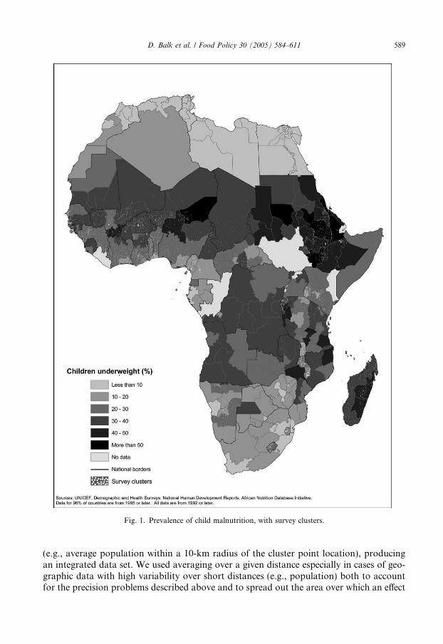
Fig. 1. Prevalence of child malnutrition, with survey clusters.


(e.g., average population within a 10-km radius of the cluster point location), producingan integrated data set. We used averaging over a given distance especially in cases of geo-graphic data with high variability over short distances (e.g., population) both to accountfor the precision problems described above and to spread out the area over which an effect

Table 2Variables derived from environmental data sets that were linked with the survey data

Variable Source Descriptiona Association withcluster pointsa

Resolution(minb)

Population

Population density CIESIN and CIAT(2003)

In persons per km2 ofland area

Averaged within a10-km radius ofthe cluster point

2.5

Urban proximity Based on CIESIN et al.(2004) urban areas data

Modelled travel time inhours to nearest town ofpopulation >25k, >50k,>100k and >500kwithout crossing wateror international borders

Averaged within (A)10 km and (B) 25 km

0.5

Conflict CIESIN, unpublisheddata, based onGleditsch et al. (2002)

Number of calendaryears with politicalconflict of high, mediumand low intensity, since1975 and 1990

Value at cluster point 30

Infrastructure

Seaport proximity Based on World Bankdata

Distance to nearestport of any size (km)

Value at centre ofquarter-degree gridcell containing clusterpoint

15

Road density Based on NIMA (1995) In km of roads perkm2 of land area

Within 100-km radius n/a

Climate and cropping

Cropping intensity Ramankutty and Foley(1998)

Percentage of 5-mincell cropped

Averaged within (A) 10-km, (B) 25-km and (C)50-km radius

5

Pasture intensity Unpublished data fromFoley et al. (2003)

Percentage of 5-mincell in pasture


5

Tree cover density DeFries et al. (2000) Percentage of half-mincell with tree cover


5

Cereal production IFPRI, unpublisheddata, based onRamankutty and Foley(1998) and FAO (2003)

In calories per capita (A) value at clusterpoint, (B) averagedwithin 25-km radius

5

Average rainfall IIASA-FAO (2000) In mm Value at cluster point 30Length of growingperiod

IIASA-FAO (2000) In months Value at cluster point 30

Farming systema Dixon et al. (2001) Classes Value at cluster point n/aSoil constraints IFPRI, unpublished

data, based on Sanchezet al. (2005) and FAO(1995)

Percentage of 5-mingrid cell with low CEC(high leachingpotential), aluminiumtoxicity, low potassiumreserves, shallow orgravelly, or organic soils

Values at cluster point(one for eachconstraint)

5

Physiography

Elevation Rabus et al. (2003) In m above sea level Value at cluster point 0.5Slope Rabus et al. (2003) In % Value at cluster point 0.5


Table 2 (continued)

Variable Source Descriptiona Association withcluster pointsa

Resolution(minb)

Roughnessa Nelson, unpublisheddata, 2001

Classes based onMeybeck et al. (2001)

Value at clusterpoint

5

Disease ecology

Index of stabilityof malariatransmission

Kiszewski et al.(2004)

Composite ofepidemiologicaland environmental data

Value at clusterpoint

30

a Some variants were removed during preliminary variable selection in favour of other variables listed.b 1 min is approximately equal to 1.85 km at the equator.


might occur hypothetically. For example, spatially discrete phenomena, such as cropland,are likely to spill over in important ways (e.g., through economic activity and diseasetransmission) into nearby non-agricultural areas.

Sampling and data quality considerations

The DHS data have been widely used in health and mortality studies (IRD-Macro Intl,1991); nevertheless, DHS are broad-scale and cross-sectional, not customized, a priori, toa given research question. As a result, the sampling frame or set of questions on a partic-ular topic may have some shortcomings for the question at hand. In this study, two suchissues arose.

All children were selected for the survey by virtue of being born to women who wereresident in surveyed households. It is important to note that children not living in the samehousehold as their biological mothers, including orphans and foster children, were not sur-veyed. This is a concern since orphans and foster children, because they live either in insti-tutional settings or other family arrangements that may already be vulnerable, may receivefewer nutritional, educational and health investments than children who reside in house-holds with their biological parents. In a recent study of Rwanda, Siaens et al. (2003) foundsignificant differences between orphans and non-orphans in terms of school enrolment,child labour and malnutrition rates, among other outcomes.

Some recent DHS, including those carried out since 1999 in Ethiopia (CSA, ORCMacro, 2001), Mali (CPS-MS, DNSI, ORC Macro, 2002) and Namibia (MOHSS,2003) and two others not included in this study population,10 measured all children resi-dent in surveyed households, but most surveys in this sample did not. Namibia is the onlycountry among these where children not living with their mothers have significantly lowerweight-for-age Z scores than children living with their mothers. Because Namibia has thegreatest percentage of such children among this set of countries, it is also possible that thisis a sample-size effect.11 Thus, while the potential for bias is noted, significant findings

10 Eritrea (NSEO-ORC Macro, 2003) and Zambia (CSO, CBH, ORC Macro, 2003) are not included in thisportion of the study.11 AIDS has been documented to cause a wide range of development challenges (Sachs, 2005), in part through itsincrease of fragmented homes. HIV/AIDS prevalence is significantly higher in Africa than anywhere else in theworld, perhaps acting as incentive for the DHS to include children who do not reside with their biological mother(although they do not include children residing in institutions). Of these five countries, Zimbabwe (33.7%),Namibia (22.5%) and Zambia (15.6%) have high prevalence of HIV, but Eritrea (2.8%) and Mali (1.7%) do not(World Bank, 2004).

Table 3Category variables used in Phase 1, individual analysis of underweight children

Variables Rural only(% of sample)

Urban and rural(% of sample)

Country of origin

Burkina Faso (reference category) 2.63 2.39Benin 1.18 1.39Central African Republic 0.95 1.29Cote d�Ivoire 4.26 5.29Cameroon 4.43 4.83Ethiopia 18.24 16.09Ghana 3.78 4.11Guinea 1.08 1.25Kenya 10.96 10.43Madagascar 6.05 6.05Mali 2.62 2.76Malawi 3.26 2.97Nigeria 21.59 22.18Niger 5.07 4.79Namibia 0.34 0.39Chad 1.81 1.80Togo 1.59 1.63Tanzania 8.09 7.95Zimbabwe 2.09 2.40

Family characteristics

First born 18.23 19.45High birth order 38.91 36.49Twin 1.98 2.06Male 50.05 50.21Mother is head of household 8.83 8.78

Maternal schooling

No schooling 57.15 52.19Attended primary school 33.05 33.41Attended secondary school 9.80 14.40Mother is unemployed 28.33 29.32Mother has skilled employment 4.08 4.80

Household characteristics

Electricity 5.54 16.37Radio 43.20 49.41Television 4.11 10.69Well water 49.36 43.09Surface water 37.86 31.57Flush toilet 0.76 4.67No toilet 52.70 44.44Household has finished floor 24.12 34.03Child has been fully vaccinated by age 1 37.34 42.01Child had a fever in the past 2 weeks 40.37 39.21

Length of growing period

Between 120 and 299 days 65.51 65.99Too short (fewer than 120 days) 14.54 13.60Too long (more than 299 days) 19.94 20.42

Urban residence 20.67


Table 4Continuous variables used in Phase 1, individual analysis of underweight children

Variables Rural only Urban and rural

Min Max Mean Min Max Mean

Family characteristics

Birth weight 1 5 3.15 1 5 3.18Percentage of household under age 5 0 75 32.23 0 75 32.02Child�s age (months) 12 35 22.85 12 35 22.84Mother�s age 15 49 28.49 15 49 28.36Children ever born to mother 1 18 4.25 1 18 4.11Percentage of mother�s children that died 0 86 12.38 0 86 11.37

Land characteristics

Sandy soil 0 100 10.23 0 100 10.15Aluminium toxicity 0 100 21.02 0 100 21.40Low nutrient reserves 0 100 34.32 0 100 34.89Shallow soil 0 100 12.96 0 100 12.41Soil type is organic 0 17 0.56 0 17 0.57Elevation 0 3814 906.63 0 3814 850.18Slope 0 1765 155.45 0 1765 141.84Precipitation (average daily rainfall mm) 22 3165 1225.29 22 3165 1234.35Per capita production within 25 km 0 44,311 77.98 0 44,311 80.52Tree cover (% within 10 km) 0 70 16.60 0 70 16.01Pasture (% within 10 km) 1 88 38 1 88 37.00Cropland (% within 10 km) 0 84 16.85 0 84 16.20

Other

Malaria (stable transmission index) 0 38 13.22 0 38 13.76Population density, (measure) 0 3762 173.74 0 11440 427.55Distance (km, straight line) to nearest port 2 1813 504.28 1 1813 477.92Distance to nearest town of >25k persons 0 89 8.53 0 118 7.36


occur in only one of five countries. We recommend that future data be collected so as totest for this bias more completely.

Anthropometry data availability varies widely between countries. In the anthropometrysample in Guinea, 41% of children have no valid measurement data, while in Nepal thisrate is only 4%. Children may lack valid data for several reasons: they could be absentfrom home at the time of the survey, their mothers could refuse permission for their mea-surement or some combination of height, weight and age values could be sufficientlyimplausible as to cast doubt on all measurements for the child. We assume no systematicbias is associated with these omissions.

A child�s underweight status reflects both short- and long-term effects of inadequate die-tary intake and the effects of infectious diseases, short-term shocks such as floods,droughts and conflict or a good rainfall year, as well as longer-term political and economicstability at the time that DHS were conducted. The environmental variables used in thisanalysis represent long-term or predominating conditions, rather than short-term fluctua-tions. Some of these variables are known to have considerable temporal variation (e.g.,climate) whereas others (e.g., soils, elevation and slope) are not expected to change mark-edly over the short or medium term. Although the DHS rarely field a survey during timesof crisis, they often implement one when a country is in a rebuilding period. Future studies


should consider the impact of time-varying variables with known spatial specificity,namely climate variability and political conflict.

Methodology

We undertook a simple ordinary least squares (OLS) regression analysis to test hypoth-eses from the UNICEF framework. Incompatibility across surveys constrained the vari-ables selected for analysis. Tables 3 and 4 describe the variables included in theanalysis. The outcome variable used was Z scores of weight-for-age of children; weassigned children whose weight-for-age was more than 2 standard deviations (SD) abovethe mean a score of 2 SD above the mean in order to remove any impact of overweightchildren, for whom the model is not designed. We further restricted the analysis to childrenaged 1–3 because below that age, and particularly below 6 months, they may have moreerror in their anthropometry. Also, they had censored observations on some of the explan-atory variables (e.g., vaccination rates, because children under age 1 are not required to befully vaccinated based on WHO guidelines). Children above age 3 were not surveyed insome countries.

We inverted and rescaled the weight-for-age scores so that the least underweight childwas assigned a score of 0 and the most underweight had a score just below 8. Thus, posi-tive covariates in the regression correspond to high shares of underweight children andnegative covariates are interpreted as being associated with lower shares of underweightchildren. We tested results for this scaled index against results for the raw Z scores, andthey showed no significant difference, thus, the regression results reported here use thescaled index because they are easier to interpret. In addition, we tested the models usingheight-for-age Z scores (scaled and unscaled). These results are summarized in the textbut not in the tables.

All households in a given EA have the same values of georeferenced variables. Becauseof this and the complex sampling frame, we used OLS regression with a cluster flag inStata to account for possible spatial error.12 We ran various models for hypothesis testingwhereby poorly performing, and then ultimately potentially endogenous variables areremoved from the final equation.

Results

Table 5 shows the results of these regressions. Models 0–6 were conducted using onlyrural children to maximize the potential impact of some of the agro-climatic variables.Model 0 shows the differences among underweight children by country. With BurkinaFaso as the reference category, Chad, Mali and Madagascar experience the same levelsas do children in Burkina Faso, and children in Zimbabwe experience the most favourablerelative circumstances. Countries are again controlled for in Model 6 and much of the var-iation in the underspecified Model 0 will be accounted for by variation in socio-economic,demographic and spatial factors that differ across the countries of the study region.

12 The technique was successfully used elsewhere (Balk et al., 2004) and accounts for the complex samplingframe. This model specification is a first-order attempt to account for cluster-specific spatial autocorrelation but amore formal spatial regression is not specified here, as it is the subject of ongoing work. At this scale, thespecification of spatial regression has proven challenging to implement in the existing spatial regression softwarepackages.


The variables introduced in Model 1 are basic demographic characteristics of each childand, except for child age, are exogenous to the child but are necessarily intended as morethan control variables. Older children are less likely to be underweight (Madise et al.,1999). However, unlike previous work, quadratic or logarithmic relationships (tested inmodels not shown) were not significant. We expected children born as a multiple birth(e.g., twins or triplets) to be more underweight, even in this age range, given the strongassociation exhibited by this variable on childhood mortality in the region (Balk et al.,2004). While we found no significance for this variable in Model 1, we retained it in latermodels, in which it becomes evident that twins tend to be more underweight than otherchildren. Similarly, children in high parity births, who may also need to compete dispro-portionately for resources, are more likely to be underweight. We expected that male chil-dren would be less underweight than female children because evidence shows thatdaughters receive fewer investments on average and therefore we expected they wouldreceive fewer nutritional ones as well. However, the regression results suggest just theopposite, reiterating surprisingly widespread evidence from other studies (Madise et al.,1999; Charmarbagwala et al., 2004). Nutrition experts also have suggested that such dif-ferences may be hard to observe (Kativa Sethuraman, personal communication, December2003).13 This effect persists throughout the models. Lastly, the proportion of the house-hold that is under age 5 in a household positively correlates with their underweight status.Two potential explanations are likely. More children can translate into more competitionfor food, and fewer adults per child means less labour supply.

In our initial Model 1, we included a term for the duration of breast-feeding, expectingthat breast-feeding would exhibit a strong protective effect against children being under-weight, as has been demonstrated widely in the literature (Van Landingham et al., 1991;Menken and Kuhn, 1996). However, we observed the contrary: the longer a motherbreast-feeds her child, we found, the greater the likelihood that the child is underweight.We determined that this effect was likely due to endogeneity, a finding with which otherstudies have also had to come to terms. Engle et al. (1999) find, for example, that educa-tion increases the mother�s opportunity cost and reduces her duration of breast-feeding.Further, to the extent that long-duration breast-feeders are poorer than other women (Osi-nusi, 1987; Perez-Escamilla et al., 1999), they may not be able to provide the same supple-mental foods to their children as other women, and themselves may be poorly nourished,leading to lower-quality breast milk. Thus, breast-feeding was not accounted for in modelsreported in Table 5.

Model 2 includes maternal characteristics. Increases in mother�s age are inverselyrelated to underweight status. One interpretation of this is that experience matters,although whether that is specifically maternal experience is not clear. The effect is margin-ally more important at younger ages, as expected, with a logarithmic specification per-forming marginally better than a linear one. The children born to mothers who haveexperienced high child mortality of their own children have much greater chances of beingunderweight. Education, both primary and secondary, exhibits strong downward pressureon being underweight.

13 Garg and Morduch (1998) suggest that gender effects are observed with birth interval, and gender ofsucceeding births is accounted for, whereby sisters of brothers fare comparably worse than sisters of sisters.

Table 5Child-level regression coefficients predicting underweight status

Models

0 1 2 3 4 5 6 7 (6 + urban) 8 (stable)

Country dummies (ref. = Burkina Faso)Benin �0.494** �0.211** �0.214** �0.229**Central AfricanRepublic

�0.363** �0.218* �0.154� �0.196**

Cote d�Ivoire �0.464** �0.155� �0.191** �0.209**Cameroon �0.711** �0.273** �0.245** �0.274**Ethiopia 0.163** 0.065 0.035 0.157**Ghana �0.452** �0.044 �0.027 0.011Guinea �0.541** �0.211* �0.158* �0.160*Kenya �0.681** �0.500** �0.491** �0.402**Madagascar 0.030 0.309** 0.332** 0.314**Mali �0.026 �0.067 �0.107� �0.132*Malawi �0.467** �0.281** �0.288** �0.284**Nigeria �0.145� 0.009 0.075 0.070Niger 0.412** �0.086 �0.065 �0.154�

Namibia �0.540** �0.434** �0.359** �0.438**Chad 0.042 �0.197** �0.165** �0.217**Togo �0.410** �0.183* �0.184** �0.188**Tanzania �0.263** �0.128 �0.097 �0.032Zimbabwe �0.959** �0.638** �0.569** �0.560**

First born �0.051High birth order 0.138** 0.121* 0.124** 0.126**Twin 0.122 0.268� 0.324** 0.333**Birth weight �0.215** �0.157** �0.172** �0.172**Sex �0.124** �0.109** �0.114** �0.112**Percentage ofhouseholdunder age 5

0.005** 0.179 0.174� 0.176�

Mother is head ofhousehold

�0.079� 0.105** 0.070* 0.077*

Child�s age (months) �0.007** �0.004* �0.004* �0.004*Mother�s age (log) �0.370** �0.203* �0.254** �0.255**

596D.Balk

etal./FoodPolicy

30(2005)584–611

Maternal schooling (ref. = none)Attended primary school �0.377** �0.104** �0.094** �0.103**Attended secondary school �0.698** �0.308** �0.318** �0.330**

Mother is unemployed 0.111** 0.065* 0.047� 0.050�

Mother has skilled employment 0.057Children ever born to mother 0.015�

Percentage of mother�schildren that died

0.004** 0.202* 0.173* 0.181*

Electricity �0.203* �0.142* �0.130** �0.132**Radio �0.228** �0.123** �0.120** �0.122**Television �0.107Water/sanitation

principal component 10.042** �0.017 �0.008

Water/sanitationprincipal component 2

0.042* �0.014 0.006

Household has finished floor �0.205** �0.091* �0.102** �0.103**Child has been fully

vaccinated by age 1�0.285** �0.064* �0.067** �0.072**

Child had a fever inpast 2 weeks

0.201** 0.202** 0.181** 0.182**

Soil characteristicsSandy 0.004** 0.003* 0.002* 0.002*Aluminium toxicity 0.001Low nutrient reserves �0.002� 0.000 0.000Shallow 0.000Type is organic �0.068** �0.016� �0.016*

Length of growing period(ref. = 120–299 days)

Too short (<120 days) 0.275** 0.087 0.103� 0.128*Too long (>299 days) 0.101* 0.115* 0.093* 0.096*Elevation (1000 m) 0.099** 0.002 0.020Slope 0.000Precipitation (average

daily rainfall, mm)0.036

Per capitaproductionwithin 25 km

0.000

D.Balk

etal./FoodPolicy

30(2005)584–611

597

(continued on next page)Table 5 (continued)

Models

0 1 2 3 4 5 6 7 (6 + urban) 8 (stable)

Tree cover (% within10 km)

�0.008** �0.003� �0.004** �0.004**

Pasture (% within10 km)

0.003* 0.322 0.251 0.365*

Cropland (% within10 km)

0.005** 0.005** 0.005**

Malaria (stabletransmissionindex)

0.002

Population density(1000 people/km2)

�0.151� �0.071 �0.003

Distance (1000 kmstraight line) tonearest port

0.571** 0.303** 0.253** 0.265**

Distance (km) tonearest townof >25 K persons

0.001

Urban residence �0.136** �0.143**Constant 4.045** 4.685** 5.111** 4.034** 3.620** 3.555** 4.969** 5.217** 5.219**R2 0.075 0.040 0.053 0.061 0.068 0.022 0.154 0.178 0.176F 68.91 31.29 46.54 55.63 33.82 34.2 42.65 60.70 69.51Number ofobservations

25,674 25,448 25,674 24,882 25,667 25,671 24,673 33,655 33,658

Significant at �p < 0.1, *p < 0.05 and **p < 0.01.

598D.Balk

etal./FoodPolicy

30(2005)584–611


Model 3 controls for household-level socio-economic characteristics, and those repre-senting health investments. Children in households that were electrified and had radioswere less likely to be underweight, not surprisingly, although we observed no effect basedon television ownership. We found similar downward pressure on underweight status inhomes with finished floors. Because of high correlation between data on water and sani-tation, we combined sources into two indices using principal components. The first com-ponent is correlated positively with well water and negatively with surface water. Thesecond is correlated positively with the complete lack of toilet facilities and negatively withflush toilets. Both were significant in the direction expected. However, neither is significantin fuller models.

Children who were fully vaccinated by age 1 were less likely to be underweight, presum-ably both because they are healthier and because they have parents who are more proac-tive in terms of direct health investments. Analogously, children who had experiencedrecent fever were more likely to be underweight. A recent fever is assumed as indicationof the child�s more general health status, although there are no other ancillary data inthe data set to confirm this.

Model 4 introduces soil fertility constraints and other environmental variables. Wetested four variables describing physical and chemical soil characteristics in this modelas well as whether the soil type was organic (i.e., characterized by wetness, low bulk den-sity and low fertility, particularly nitrogen and micro-nutrient deficiencies). These soil vari-ables were considered to be the most distinctively difficult for food production (PedroSanchez, personal communication, May 2004). Children living in areas with soils that havelow nutrient reserves or are sandy are more likely to be underweight, with a much strongereffect being observed on sandy soils. Additionally, as we expected, soils with high organiccontent were found to be associated with lower levels of underweight children.

We also included length of growing period (LGP) in the model. Children living in areaswith growing periods that were either very short (fewer than 120 days) or very long (morethan 299 days) were more likely to be underweight than children living in areas with moreoptimal growing periods, consistent with our expectations. Agro-ecological zones withvery short or very long LGP (due to rot) do not produce enough food; therefore, agricul-tural communities living in these areas may face food shortages and malnutrition.

Elevation is also associated with being underweight but average terrain slope showedno effect. Children living in areas with more tree coverage were less likely to be under-weight but, counter to our a priori expectations, children living near pasture and croplandwere more likely to be underweight. We know that cultivated areas tend to be more den-sely populated than other rural areas (McGrahanan et al., in press), a variable that is inde-pendently included in subsequent models. We asked whether farming systems categoricallydiffer in their socio-economic characteristics, for example, whether educated families areless likely to live in the most vulnerable systems (either because they have migrated to lessvulnerable ones, or because those regions have fewer schooling opportunities). Althoughthere are statistically significant differences in mother�s educational level by farming system(not shown), mothers with the highest average education were found in a wide range offarming systems (e.g., both rice-tree cropping and sparse agriculture) dismissing concernover potential self-selection.

Aside from these direct agro-climatic conditions, a few additional spatial variables areentered in Model 5. These include an index of the stability of malaria transmission risks(Kiszewski et al., 2004), population density and distance to the nearest port and city of

Fig. 2. Average regional weight-for-age Z scores, actual values.


25,000 persons or more. Of these, only population density (weakly) and nearness to port(strongly) were associated with not being underweight. We assume that the populationdensity captures a large degree of urbanness and thus reduces the likelihood of an indepen-dent effect of nearness to an urban centre. The malaria transmission index showed noeffect. The coarse (half-degree) resolution of the data may have reduced any potentialeffect.14

Model 6 enters all variables that showed an effect significant at the 0.1 level in earliermodels (including some of those discussed as flawed or with unexpected effects above)as well as all the country dummies. While some variables are no longer significant (e.g.,elevation), most are simply dampened by the complexity of the model. Once controllingfor many covariates, nearly all the country dummies exhibit weaker and less significanteffects.

The Model 7 regression was run on a fuller subsample of the data – urban and ruralchildren in the same age range. In this model, a dummy variable for urban dweller wasincluded. As expected, urban children are less likely to be underweight than their ruralcounterparts. All other significant regressors from Model 6, even the soil modifiers, remainsignificant (some more, others less) in Model 7.

In preparation for Phase II of this study, we generated Model 8, in which endogenousand unexplainable variation (as well as variables that would be conceptually meaninglessat the meso-scale) was removed from Model 7. This has the overall impact of slightlyreducing the significance of the overall model (i.e., the R2, or explainable variance term)but provides a stable and unbiased estimate of underweight children at the micro-levelfor comparison with the meso-scale analysis.

14 An analysis of mortality had similar findings showing a strong bivariate relationship with the malaria indexbut a significant relationship in the multivariate model was not sustained, partly due to the strong co-linearitywith other country-level control variables (Balk et al., 2004) due to the coarseness of the index. Future studiesshould use more highly resolved data, if and when they become available.


Using height-for-age Z score as the dependent variable instead of weight-for-age pro-duced similar but weaker results in the eight models (not shown). The only factors forwhich the direction of a significant effect changes are country dummies. In general, fewereffects are significant and more weakly so. Mother�s primary education, proximity to ports,vaccinations, tree cover and mothers heading households all lose much or all of their sig-nificance in most or all of the models in which they appear. Multiple births, however, aremore significantly correlated with low height-for-age scores. The effects of elevation andthe malaria transmission index also become significant, although in the unexpecteddirection.

To summarize the child-level analysis, numerous factors emerged as clearly significant.In general, those operating at the household level showed clearer effects than those at theenvironmental level. The specification of this model and its associated data, however, didnot allow us to determine whether households are effective mediators of environmentalrisk. For example, elevation has no effect when household socio-economic variables areincluded, presumably because most of those with significant resources have been able tomove to more favourable (i.e., lower) elevations. It is also plausible that there is far lessmeasurement error in the household variables for which the survey instruments weredesigned than in the geospatial variables, which were originally measured for differentunits and purposes and associated with the surveyed regions through a complex andimperfect process. If the latter were true, the geospatial variables would perform betterin a meso-level analysis where such imprecision can be tolerated.15

Phase II. Meso-level analysis of determinants of underweight children in Africa, Asia and

Latin America

In this phase, we aggregated variables for all children to the subnational survey regionin which they lived and then undertook regressions. Because we did not require precisespatial information on the location of the household, this analysis included data fromcountries that did not have the EA location information needed for the analysis in PhaseI. Thus, the Phase II analysis incorporates regions in several countries in Asia and LatinAmerica as well as additional countries in Africa. To make the results as comparable aspossible to those from Phase I, we only worked with rural households.16 To reduce stan-dard errors, we omitted subnational regions where fewer than 50 children have valid data.This left 319 subnational units, drawn from 45 countries (Fig. 2). Because we are notattributing regional-level associations to individual-level phenomena but rather character-izing relationships strictly at the regional level, the ecological fallacy is not a critical prob-lem (Schwartz, 1994; Diez Roux, 2004).

Data

In this phase, the outcome variable is the average weight-for-age Z score among chil-dren aged 1–3 in each region. As in Phase I, children who were more than 2 SD above

15 Because so few differences emerge between the wasting and stunting analyses, we did not conduct a meso-scaleanalysis using stunting as the malnutrition indicator.16 This is not to suggest that urban malnutrition is not an important issue, rather just one that cannot be as wellspecified in the meso-scale analysis as it could have been in the individual-level analysis with more geographicinformation.

Table 6Aggregate-level regression results predicting underweight conditions in subnational regions

Model

0 1 2 3 4 5 6 7 8 9

Country dummies (ref. = India)Bangladesh 0.222� �0.090 0.065Benin �0.415** �0.446* �0.166Bolivia �1.016** �0.935** �0.527**Brazil �1.158** �0.865** �0.610*Burkina Faso 0.095 �0.208 0.157Cambodia 0.092 �0.034 0.169Cameroon �0.807** �0.577** �0.338*Central African Republic �0.278* �0.629** �0.263�

Chad 0.195* �0.419 �0.129Colombia �1.116** �0.286 �0.140Comoros �0.456* �0.170 �0.376Cote d�Ivoire �0.348** �0.763** 0.055Dominican Republic �1.465** �1.168** �0.732**Egypt �1.751** �0.072 �1.029**Eritrea 0.345* �0.455** 0.011Ethiopia 0.177� �0.360� �0.268*Gabon �0.825** �0.376� �0.099Ghana �0.321** 0.151 �0.035Guatemala �0.267* �0.630** 0.118Guinea �0.460** �0.645** �0.451*Haiti �0.823** �0.718** �0.718**Kazakhstan �1.583** �1.824** �1.305**Kenya �0.601** �0.473** �0.197Kyrgyz Republic �1.199** �1.374** �0.840**Madagascar 0.020 �0.073 0.132Malawi �0.474** �0.553** �0.237Mali 0.050 �0.367� �0.003Morocco �1.156** �0.912** �0.751**Mozambique �0.331** �0.519** �0.287*Namibia �0.503** �0.617** �0.115Nepal 0.211 0.034 0.066

602D.Balk

etal./FoodPolicy

30(2005)584–611

Nicaragua �1.045** �0.734** �0.606**Niger 0.448** �0.286 0.030Nigeria �0.055 �0.136 0.161Pakistan 0.031 �0.299� �0.223Peru �0.965** �0.591** �0.434**Rwanda �0.454** �0.514** �0.388**Tanzania �0.162 �0.167 0.095Togo �0.330* �0.342 �0.018Uganda �0.500** �0.656** �0.340*Uzbekistan �1.095** �1.111** �0.645**Zambia �0.352** �0.550** �0.146Zimbabwe �0.860** �0.783** �0.422**

HH size factor 1 �0.047 �0.091** �0.078** �0.084**HH size factor 2 �0.206 ** �0.055* �0.074** �0.041�

Fraction mothers headof HH

�0.660 �0.174

High-fertility index 0.295** 0.057Average mothers age �0.078** �0.010 �0.052** �0.007Fraction mothers withprimary education

�0.841** �0.598** �0.734** �0.698**

Fraction mothers withsecondary education

�1.311** �0.204 �0.520** �0.567**

Fraction mothers inskilled employment

�0.007 0.357

Fraction mothersunemployed

�0.665** �0.091

Asset index 1 �0.288** �0.138* �0.324** �0.131*Asset index 2 �0.359** �0.190** �0.342** �0.237**Fraction children fullyvaccinated

�0.408** �0.070

Fraction children withfever near survey

0.220 0.063

Sandy soil (%) 0.012** 0.003 0.004* 0.003�

Territory with growingseason >300 days (%)

�0.271* �0.099

Territory with growingseason <120 days (%)

�0.608** 0.013

D.Balk

etal./FoodPolicy

30(2005)584–611

603

(continued on next page)Table 6 (continued)

Model

0 1 2 3 4 5 6 7 8 9

Fraction of territory with trees �0.010** 0.000Average elevation (1000 m) �0.003 0.089�

Average slope 0.007 �0.028*Average food production (kcal per capita) �0.005** 0.002Average Malaria Index 0.019** 0.002 0.011** 0.000Pop density 0.546� 0.087 0.176* 0.121Average distance to nearest port 0.020* 0.016Fraction of territory occupied by small

urban areas0.015** 0.005* 0.001

Fraction of territory occupied by mediumurban areas

�0.001

Fraction of territory occupied by largeurban areas

0.000

Fraction of territory within 2 km of road �0.843* �0.219Fraction of territory within 15 km of road 0.356 0.023Fraction of territory near railroad �1.729� �0.444Density factor 1 (high density, lots of

small urban areas)�0.126 0.015

Density factor 2 (large urban areas) �0.117Political conflicts since 1975 (low intensity) 0.043� 0.013Political conflicts since 1975

(medium intensity)�0.003 0.015 0.019** �0.006

Political conflicts since 1975 (high intensity) 0.020* 0.009Political conflicts during 1990s (low intensity) �0.068* �0.033Political conflicts during 1990s

(medium intensity)0.001 �0.050

Political conflicts during 1990s (high intensity) �0.068� �0.026(Constant) 3.980** 3.518** 6.521** 3.570** 3.922** 3.084** 3.461** 4.491** 5.069** 4.249**R2 0.831 0.119 0.369 0.638 0.265 0.233 0.033 0.903 0.769 0.889F 31.38 10.63 36.67 138.5 15.63 10.15 1.73 27.77 82.08 37.08

Significant at �p < 0.1, *p < 0.05 and **p < 0.01.

604D.Balk

etal./FoodPolicy

30(2005)584–611


the mean were re-coded; and the scores were inverted, so that high scores corresponded tohighly underweight conditions, and adjusted arithmetically so that their lowest value waszero. Thus, for example, a score of 0 corresponds to 2 SD or more above the mean, and ascore of 3 would correspond to 1 SD below the mean. The outcome variable for the sub-national units in the study ranged from 1.4 to 5.0, with a mean of 3.5. This outcome var-iable correlates quite highly with the percentage of all children who are more than 2 SDbelow the mean (i.e., Pearson�s correlation coefficient is 0.96).

We calculated subnational aggregations of all the relevant variables tested in Phase I.For example, the Phase I variables that indicate the mother�s educational status wereaggregated to two variables that indicate the percentage of mothers in the region withsome primary education and the percentage with some secondary education. For theseeducational variables, the aggregated versions are directly analogous to the household-level counterparts. In other cases, however, the variables need to be interpreted in a differ-ent light when aggregated. Birth order, for example, serves as a child-level control variablein the Phase I study. A child who enters the family as the fifth child or higher is signifi-cantly more likely to be underweight than a child who is not. At the subnational level,the aggregation of this variable serves not as a control variable for individual risk butrather an indicator of fertility levels within the region.

We found that, for the subnational aggregates, measures that were substantivelyrelated often performed poorly when entered into a regression together. This was par-ticularly so for the household asset measures; although each was separately negativelycorrelated with underweight outcomes, when combined some became positively corre-lated. We therefore investigated principal components for functionally related variablesand used factor scores in lieu of individual variables in some cases. We calculated twohousehold asset indicators using principal component analysis. We further found thatmany of the control variables in the Phase I analysis served essentially as indicatorsof household size and composition at the regional level, and thus calculated two princi-pal components, which we designated HHSize1 and HHSize2. Lastly, we calculated ahigh-fertility index by using the factor loads from two variables, the percentage of chil-dren who are first-born and the percentage of children who are fifth-born or higher. Weopted for this rather than for measuring the total children ever born to the mother toaccount a bit more for distributional effect than simply the average total fertility in theregion.

Methodology

We sought to explain the variation in the underweight measure using a sequence of OLSregression models emphasizing different sets of drivers in the same manner as Phase I,except that here we treated each subnational region as an independent observation. Wethen combined the drivers into a single model and finally estimated a model with only sta-tistically significant factors. This latter model constitutes a composite risk model, whereasthe others identify risks associated with specific factors.

Results

Table 6 summarizes results. Model 0 shows the degree to which national dummy vari-ables can account for differences at the level of the subnational unit. Largely because theaverage country has only 7.25 subnational units, the country dummies perform quite wellin this model, accounting for 83% of the variance.


Model 1 considers the effect of regional demographic structural factors. Regions withlarge households have fewer underweight children. This is consistent with findings fromthe economic demography literature showing that large households are better equippedto pool risk than are smaller households (e.g., Townsend, 1994). We also find here thatregions with high fertility have more underweight children; again this is consistent withprevailing understanding. Altogether these factors account for 12% of the variance.

In Model 2, maternal attributes are explored. Education plays a major impact, asexpected. The proportion of mothers with some primary education reduces underweightstatus, as does the proportion with some secondary education. We find that the averageage of mothers is negatively associated with underweight status, which is consistent withPhase I findings. In this model, however, maternal unemployment unexpectedly alsoreduces underweight status. Whether this indicates that an underlying factor associatedwith unemployed mothers – such as regional economic factors, i.e., women may not workin wealthier regions – has an effect, requires more investigation. Model 2 accounts for 37%of the variance.

InModel 3, we explore the role of household-level investments.We find a strong effect forthe physical assets and a significant effect from vaccination rate.However, the fevermeasure,which was significant as a child-level control in Phase I, does not perform well as a regionalaggregate. Consistent with the conclusion that tangible household assets are a strong deter-minant of life prospects, this model accounts for 64% of the variance. Because of the strongassociation, we map the risk factor derived from these measures (Fig. 3).

Model 4 examines the impact of physical factors relevant to agricultural production.Because of complications in processing the soil data, we only tested one soil constraintin Phase II but would have liked to test more. We found that the percentage of a regionwith sandy soil is positively associated with underweight status. The tree-cover measurealso performed here as in Phase I. The growing season measures that performed ashypothesized in Phase I had the opposite effect in Phase II; regions with very long or veryshort growing seasons had lower underweight problems than other regions. In future tests,we would want to calculate population-weighted aggregates of growing season as ourresults here may be a function of territorial averages that do not reflect the conditions

Fig. 3. Predicted values of regional weight-for-age Z scores, wealth and health model.


under which most people actually live. For example, a region with a wet and a dry zonewill most likely have most of its people living in the wet zone; therefore, it would be mis-leading to include the dry zone�s lower growing season as a contributor to the well-being ofthe people living in the wet zone. This model altogether accounts for 26% of the variance.

Model 5 looks at other physical characteristics of the region. We find significantrelationships in the expected direction for exposure to malaria, distance from ports anddensity of road networks and railroads. For overall population density, we find thathigh-density levels are associated with higher levels of underweight status; normally urbanchildren are less underweight than rural children, which is borne out by the Phase I results.Additional sensitivity analysis is called for here. We do not yet know how consistent thepattern is across regions or whether a small number of cases, such as the high underweightvalues in India that are accompanied by high population densities, are masking a differentpattern elsewhere. Regions with a large number of small urban areas have higher under-weight status; perhaps because such regions are more likely to be experiencing settlementgrowth that is outpacing their ability to invest in necessary infrastructure, thereby placingtheir populations at greater risk. Model 5 accounts for 23% of the variance.

In Model 6, we explore the effect of political conflict in a region, using a gridded data-base of conflict that we created using the Uppsala Conflict Database (Gleditsch et al.,2002). Based on our work with a data set of global subnational infant mortality rates,we expected these variables to be significant (Levy et al., 2003); however, they did not per-form well in this test. In the results reported here, some of the variables are significant buthalf the coefficients have the opposite sign expected (which is probably a function in partof the high collinearity of these measures). We find that the single best of these measures inaccounting for underweight status is the cumulative number of medium-intensity conflicts.However, the effect of conflicts since 1975 is weak. This model overall accounts for 3% ofthe variance.

Model 7 includes all the variables used in each of the above models. It accounts for 90%of the variance in underweight status. As in the Phase I results, most of the country dum-mies remain significant. The additional variables that remain significant in this model arethe two household size factors, mother�s primary education, the two asset indices, andslope and elevation. The importance of these variables, because they are highly significanteven when controlling for everything else and when including country dummies, is arobust finding.

Our suspicion is that including country dummies obscures some of the effect of the geo-spatial variables because some of the effects of these are exerted on the country as a wholeas well as on the specific subnational regions. Countries with high malaria exposure, forexample, have higher underweight status. There is an endogenous dynamic in which spa-tial drivers such as this exert a systemic effect on a country that in turn redounds to thedetriment of regions and households, making it hard to discern precise signals in a staticanalysis of this sort. We cannot know in which cases the impact of the country dummies inbumping some variables out of significance reflects this kind of underlying dynamic andwhen it does not. Under the circumstances, we estimated Model 8, which removes thecountry dummies and retains only the remaining statistically significant variables. In thisexercise, sandy soil, malaria exposure, population density, small urban areas and medium-intensity political conflicts all become significant. The non-spatial variables that aresignificant in this model include the two household size indicators, mother�s age, botheducation measures and the two asset indicators. In some ways this model represents


our best-informed guess about the relevant risk factors faced by rural children in develop-ing countries. Even without the country dummies, the amount of variation accounted forby the model is high (77%). For the sake of completeness, we take the variables fromModel 8, bring back all the country dummies and report the results as Model 9.

Conclusions

In this study, we attempted to capture the effects of geographic and environmental vari-ables on child hunger, cross-nationally, at the household and regional levels of analysis.The strength of this approach was that such factors could be evaluated along with morecommonly found predictors of child hunger but a disadvantage was that we were unableto include a full suite of individual- and household-level variables. Future studies, either bynarrowing the geographic extent, or by improving the coverage of cross-nationally avail-able data, should attempt to include a richer set of individual-, household- and regional-level factors in the same model.

Nevertheless, we were able to pinpoint a number of household characteristics thatappear to be significant risk factors for child malnutrition. In particular, length ofbreast-feeding was inversely related to child nutritional outcomes, we argued due to aset of factors some of which we were unable to measure in this study, such as supplemen-tary feeding. The UN Millennium Project HTF advocates for breast-feeding until age 2,and this study calls for better data to evaluate supplementary feeding practices in combi-nation with nursing. The risk factors are largely consistent with prior studies, but the studyalso highlights the importance of proximity to markets, as represented by ports or urbanresidence. As no effect was found for smaller cities, consistent with the recommendation ofthe HTF it is likely that these towns and rural settlements may need extra investments ofinfrastructure, markets and so forth.

From a policy and research perspective it is noteworthy that the best-fitting modelsaccount for no more than 17% of the observed variance when all these factors are exam-ined in the household-level models. Perhaps this is not surprising for a cross-national, mul-tilevel analysis of survey outcomes that also includes externally observed environmentaland geographic factors. It is consistent with the proposition that there are interactionsbetween the factors we observe with some precision (household size, select householdassets, and so on) and factors we observe with far less precision, perhaps with complexinteractions and non-linearities, or observe not at all. As some have suggested, factorssuch as soil fertility, access to water, access to markets, availability of adequate and afford-able medical care and other spatial variables may influence patterns of poverty and hun-ger, but the evidence for such influences will be hard to observe through a staticcomparison of individual families or children. Some small-scale studies have found strongeffects from these kinds of relationships, and indeed we find that children living in regionswith suboptimal agricultural growing seasons (i.e., too short or too long) or in selectedfarming systems, for example, were more likely to be underweight. Nevertheless, our effortto look for causal relationships using micro-data on a continental scale demonstrates thatthe empirical foundation for generalizing the relative impacts of such forces is significantlylimited by an absence of adequate data, and potentially incompatibilities in the resolutionsand units of analysis of the data that do exist.

At the regional level, the broad findings that emerge from the child-level study are sup-ported on a more globally representative sample using subnational regions from more than


twice asmany countries. Thesemodels account for a greater percentage of the outcome�s var-iance. This is consistent with our proposition that household and regional dynamics interactin complicatedways that aremore difficult to discern at the individual level butwhichbecomesomewhat clearer through a regional lens. Even in the analysis that omits the country-leveldummy variables, the model�s ability to account for variation in regional underweight statusis high. In the micro-analysis, many important individual or contextual-level determinantsare omitted, whereas individual variation is masked in the regional analysis (Diez Roux,2004).One advantage of conducting an analysis at two scales is that policy recommendationscould be qualified. That is to say, regions at high risk of malaria have higher shares of under-weight children than in low risk areas. The fact that this variable was not significant at thehousehold level does not imply that a household�s individual risk of malaria is not important(and its associated consequences or co-determination ofmalnutrition), rather it suggests thatimproved specification of that risk is needed for a fuller understanding of behaviour andlikely policy effectiveness.

The following factors emerge as significant in both methods and therefore we have highconfidence that they play an important role in influencing the underweight status of childrenin developing countries: household composition and size, maternal education, householdassets and low soil fertility (as measured by sandy soil constraint). The meso-scale analysisfound that rural regions with small urban areas (as opposed to larger ones) were more likelyto have higher malnutrition, thus, reinforcing the HTF emphasis on creating viable marketsand access in predominantly agricultural areas.Riskofmalaria also appears to be important,again reinforcing the importance of diseases that affect nutritional outcomes.

In bothmicro- andmeso-scale analyses, more than any other block of variables, the influ-ence of the spatial variables is much greater in the absence of the country-level dummy vari-ables. One interpretation of this is that spatial variables provide substantive guidance toexplain country-level variation. Since countries vary considerably in environmental and spa-tially explicit features, this method provides an entry to unlocking the ways in which thesefeatures affect health and poverty outcomes, rather than simply noting differences in countryaverages. The analysis shows the potential for constructing higher-risk zones that could bepolicy targets, although no such targeting was attempted herein.

The inability to measure the effect of agricultural productivity in this analysis was anotable concern, and our meagre results in this regard reflect primarily a need to investin more appropriate data. Some progress is being made in this regard through the Agro-Maps project (http://www.fao.org/landandwater/agll/agromaps/interactive/index.jsp),but subnational data comparable across countries and dominant crops were not availableat the time of this study. Many of the variables used were imperfect proxies; superior alter-natives are in development and will shed better light on the impact such factors exert.

Finally, the differences within and between the results of micro- and meso-scale analysisclearly suggest that models which examine relationships where environmental and ecolog-ical factors are expected to be mediated by communities, households and individuals, needto refine both the data and models with which to tease apart interactions so that effectivehunger and poverty reduction strategies can be implemented.

Acknowledgements

An earlier version of this article was prepared for the HTF of the United NationsMillennium Project. We thank Jordan Chamberlain, Yunnis Yi, Audra Query, Gabriela

http://www.fao.org/landandwater/agll/agromaps/interactive/index.jsp


Fighetti and Janina Franco for assistance in the preparation of data and some of the mapsfor this study. We thank Pedro Sanchez, Lisa Dreier and Nalan Yuksel for suggestionsthroughout the project. As part of the Millennium Project HTF�s review process, we alsoreceived helpful comments from Peter Matlon, Christopher Barrett, Kostas Stamoulis andfive anonymous reviewers.

References

Balk, D., Pullum, T., Storeygard, A., Greenwell, F., Neuman, M., 2004. A spatial analysis of childhood mortalityin West Africa. Population, Space and Place 10 (3), 175–216.

Charmarbagwala, R., Ranger, N., Waddington, H., White, H., 2004. The Determinants of Child Health andNutrition: A Meta-analysis. Department of Economics, University of Maryland and Operations EvaluationDepartment, World Bank, Washington, DC.

CIESIN, CIAT (Center for International Earth Science Information Network, Centro Internacional deAgricultura Tropical), 2003. Gridded Population of the World, version 3 (alpha). CIESIN, ColumbiaUniversity, Palisades, New York. Available from: <http://sedac.ciesin.columbia.edu/gpw/>.

CIESIN, IFPRI, World Bank, CIAT (Center for International Earth Science Information Network, InternationalFood Policy Research Institute, the World Bank, Centro Internacional de Agricultura Tropical), 2004. GlobalRural–Urban Mapping Project (GRUMP): urban/rural population density grids (alpha). CIESIN, ColumbiaUniversity, Palisades, New York. Available from: <http://sedac.ciesin.columbia.edu/gpw/>.

CPS-MS, DNSI, ORC Macro (Cellule de Planification et de Statistique du Ministere de la Sante, DirectionNationale de la Statistique et de l�Informatique, ORC Macro), 2002. Enquete demographique et de sante auMali, 2001. Calverton, MD.

CSA, ORC Macro (Central Statistical Authority, Ethiopia, ORC Macro), 2001. Ethiopia demographic andhealth survey, 2000. Addis Ababa, Ethiopia and Calverton, MD.

CSO, CBH, ORC Macro (Central Statistical Office, Zambia, Central Board of Health, Zambia, ORC Macro),2003. Zambia Demographic and Health Survey 2001–2002. Calverton, MD.

DeFries, R.S., Hansen, M.C., Townshend, J.R.G., Janetos, A.C., Loveland, T.R., 2000. A new global 1-km dataset of percentage tree cover derived from remote sensing. Global Change Biology 6, 247–254.

Diez Roux, A.V., 2004. The study of group-level factors in epidemiology: rethinking variables, study designs, andanalytical approaches. Epidemiologic Reviews 26, 104–111.

Dixon, J., Gulliver, A., Gibbon, D., 2001. Farming Systems and Poverty: Improving Farmers� Livelihoods in aChanging World. United Nations Food and Agriculture Organization, Rome. Available from: <http://www.fao.org/farmingsystems>.

Engle, P., Menon, P., Haddad, L., 1999. Care and nutrition: concepts and measurement. World Development 27(8), 1309–1337.

FAO (Food and Agriculture Organization of the United Nations), 1995. Digital soil map of the world andderived soil properties, Rome, Italy.

FAO (Food and Agriculture Organization of the United Nations), 2003. Global map of irrigated areas, Version2.1, Rome, Italy. Available from: <http://www.fao.org/ag/AGL/aglw/aquastat/irrigationmap/index.stm>.

Freedman, D.A., 2001. Ecological inference and the ecological fallacy. International Encyclopaedia of the Socialand Behavioural Sciences 6, 4027–4030.

Foley, J.A., Costa, M.H., Delire, C., Ramankutty, N., Snyder, P., 2003. Green Surprise? How terrestrialecosystems could affect earth�s climate. Frontiers in Ecology and the Environment 1 (1), 38–44.

Garg, A., Morduch, J., 1998. Sibling rivalry and the gender gap: evidence from child health outcomes in Ghana.Population Economics 11 (4), 471–493.

Gleditsch, N.P., Wallensteen, P., Eriksson, M., Sollenberg, M., Strand, H., 2002. Armed conflict 1946–2001: anew dataset. Journal of Peace Research 39 (5), 615–637.

Graitcher, P.L., Gentry, E.M., 1981. Measuring children: one reference for all. Lancet ii, 297–299.Habicht, J.P., Martorell, R., Yarbrough, C., Malina, R.M., Klein, R.E., 1974. Height and weight standards for

preschool children. How relevant are ethnic differences in growth potential? Lancet 1 (7858), 611–614.IIASA-FAO (International Institute for Applied Systems Analysis-Food and Agriculture Organization of the

United Nations), 2000. Global Agro-Ecological Zones (GAEZ) 2000. CD-ROM, Rome, Italy.

http://sedac.ciesin.columbia.edu/gpw/

http://sedac.ciesin.columbia.edu/gpw/

http://www.fao.org/farmingsystems

http://www.fao.org/farmingsystems

http://www.fao.org/ag/AGL/aglw/aquastat/irrigationmap/index.stm


IRD-Macro Intl (Institute for Resource Development-Macro International), 1991. In: Proceedings of theDemographic and Health Surveys World Conference, 5–7 August, 1991, Washington.

Kiszewski, A., Mellinger, A., Malaney, P., Spielman, A., Ehrlich, S., Sachs, J., 2004. A global index of thestability of malaria transmission. American Journal of Tropical Medicine and Hygiene 70 (5), 486–498.

Levy, M., Balk, D., Storeygard, A., Booma, G., 2003. Characterizing the global distribution of poverty. In:American Association of Geographers Annual Meeting, March, 2003, Philadelphia.

Macro International Inc., 1996. Sampling manual. DHS-III Basic Documentation No. 6, Calverton, MD.Madise, N.J., Matthews, Z., Margetts, B., 1999. Heterogeneity of child nutritional status between households: a

comparison of six sub-Saharan African countries. Population Studies 53 (3), 331–343.McGrahanan et al., in press. Urban systems. In: Millennium Ecosystem Assessment: Condition and Trends, 5

vols. Island Press, Washington, DC.Menken, J., Kuhn, R., 1996. Demographic effects of breastfeeding: fertility, mortality, and population growth.

Food and Nutrition Bulletin 17 (4), 349–363.Meybeck, M., Green, P., Vorosmarty, C., 2001. A new typology for mountains and other relief classes: an

application to global continental water resources and population distribution. Mountain Research andDevelopment 21 (1), 34–45.

MOHSS (Ministry of Health and Social Services, Namibia), 2003. Namibia Demographic and Health Survey2000, Windhoek, Namibia.

NIMA (National Imagery and Mapping Agency), 1995. Performance specification: vector smart map (Vmap)level 0. MIL-PRF-89039, 9 February, Washington, DC.

NSEO-ORC Macro (National Statistics and Evaluation Office-ORC Macro), 2003. Eritrea Demographic andHealth Survey 2002. National Statistics and Evaluation Office and ORC Macro, Calverton, MD.

Osinusi, K., 1987. A study of the pattern of breast feeding in Ibadan, Nigeria. Journal of Tropical Medicine andHygiene 90 (6), 325–327.

Payne, P.R., 1990. Measuring malnutrition. IDS Bulletin 21 (3), 14–30.Perez-Escamilla, R., Cobas, J., Balcazar, H., Holland Benin, M., 1999. Specifying the antecedents of breast-

feeding duration in Peru through a structural equation model. Public Health Nutrition 2 (4), 461–467.Rabus, B., Eineder, M., Roth, A., Bamler, R., 2003. The shuttle radar topography mission – a new class of digital

elevation models acquired by spaceborne radar. ISPRS Journal of Photogrammetry and Remote Sensing 57(4), 241–262.

Ramankutty, N., Foley, J.A., 1998. Characterizing patterns of global land use: an analysis of global croplandsdata. Global Biogeochemical Cycles 12 (4), 667–685.

Sachs, J., 2005. The End of Poverty. Penguin, New York.Sanchez, P.A., 2002. Soil fertility and hunger in Africa. Science 295, 2019–2020.Sanchez, P.A., Swaminathan, M.S., Dobie, P., Yuksel, N., et al., 2005. Halving hunger: it can be done. Final

Report of the UN Millennium Project Task Force on Hunger, Earthscan, London.Schwartz, S., 1994. The fallacy of the ecological fallacy: the potential misuse of a concept and the consequences.

American Journal of Public Health 84 (5), 819–824.Siaens, C., Subbarao, K., Wodon, Q., 2003. Are Orphans Especially Vulnerable? Evidence from Rwanda. World

Bank, Washington, DC.Smith, L., Haddad, L., 2000. Explaining child malnutrition in developing countries: a cross-country analysis.

Research Report 111, International Food Policy Research Institute, Washington, DC.Tanner, J.M., 1981. A History of the Study of Human Growth. Cambridge University Press, Cambridge.Townsend, R., 1994. Risk and insurance in village India. Econometrica 61 (3), 539–591.UNICEF, 1990. Strategy for improved nutrition of children and women in developing countries, New York.UNICEF, 1998. The state of the world�s children, New York.Van Landingham, M., Trussell, J., Grummer-Strawn, L., 1991. Contraceptive and health benefits of

breastfeeding: a review of the recent evidence. International Family Planning Perspectives 17 (4), 131–136.Whitehead, R.G., Paul, A.A., 1984. Growth charts and the assessment of infant feeding practices in the western

world and in developing countries. Early Human Development 9, 187–207.WHO (World Health Organization), 1995. Physical status: the use and interpretation of anthropometry. WHO

Technical Report Series No. 854, Geneva.World Bank, 2004. African development indicators, Washington, DC.

Child hunger in the developing world: An analysis of ...

Documents

Transcript of Child hunger in the developing world: An analysis of ...