
Child Care Availability, Quality and Affordability: Are ... · Child Care Availability, Quality...
31
Child Care Availability, Quality and Affordability: Are Local Problems Related to Labour Supply? Robert Breunig ∗ Australian National University Xiaodong Gong Australian Treasury Joseph Mercante Australian Treasury Andrew Weiss Australian National University Chikako Yamauchi Australian National University Abstract We examine whether responses to survey questions about child care availability, quality, and cost, aggregated at the local geographical level, have any explanatory power in models of partnered female and lone parent labour supply. We find evidence that partnered women and lone parents who live in areas with more reports of lack of availability, low quality, or costly child care work fewer hours and are less likely to work than women in areas with fewer reported difficulties with child care. JEL CODES: J22,J30,J64, KEYWORDS: Labour supply; child care; local area effects
Transcript of Child Care Availability, Quality and Affordability: Are ... · Child Care Availability, Quality...
Child Care Availability, Quality and Affordability:Are Local Problems Related to Labour Supply?
Robert Breunig∗
Australian National UniversityXiaodong Gong
Australian Treasury
Joseph Mercante
Australian Treasury
Andrew Weiss
Australian National University
Chikako YamauchiAustralian National University
Abstract
We examine whether responses to survey questions about child care availability,quality, and cost, aggregated at the local geographical level, have any explanatorypower in models of partnered female and lone parent labour supply. We findevidence that partnered women and lone parents who live in areas with morereports of lack of availability, low quality, or costly child care work fewer hoursand are less likely to work than women in areas with fewer reported difficultieswith child care.JEL CODES: J22,J30,J64,KEYWORDS: Labour supply; child care; local area effects

I Introduction
There is broad-ranging concern in Australia about the availability, quality, and price
of child care. There have been calls (see ABC, 2009) for additional public funding to
increase availability and affordability of child care, particularly following the collapse of
ABC Learning1, a large private child care centre operator. The public debate is often
framed around the need for child care policy to be focused on allowing (sometimes even
encouraging) women with young children to enter the labour force (see ABC Radio,
2006). Policies such as Child Care Tax Rebate and Child Care Benefit provide subsi-
dies for child care usage primarily for work-related purposes. Australian Human Rights
Commission (2009) tells women that “childcare can be expensive and hard to get.” Thus,
“it is important to think about childcare while you are pregnant to make sure that you
can access childcare when you return to work.” The Parliament of the Commonwealth
of Australia (2006) documents reported problems with quality, accessibility and afford-
ability of child care in Australia and worried about “its impact on women’s ability to
participate in paid work at an optimum level.”
Clearly the availability and quality of child care, in addition to price, could affect
parental decision-making about labour supply, particularly in the highly subsidised and
regulated child care market. On the one hand, child care is a cost of working. However,
parents rarely approach the problem of finding child care as a simple cost-minimisation
exercise. Rather, child care is viewed as an important input to child development.
Parents who might want to work will be unwilling to leave their child in a poor child
care environment. Furthermore, parents who have decided to work and to place their
child in care might be willing to spend more than the minimum in order to place their
child in high-quality care, available at a convenient location.
But whether availability, quality and affordability of child care are empirically sig-
nificant issues in Australia in preventing parents from working is not so obvious and
there is a paucity of empirical research in Australia which comprehensively investigates
these multiple aspects of child care. This paper makes some progress in identifying the
role that availability and quality, along with cost, might play in labour supply choices
of partnered women and lone parents.
We simultaneously examine these multiple aspects of child care using the Household,
2
Income and Labour Dynamics in Australia (HILDA) survey which asks some respondents
about child care availability, quality, and cost. We expect that in areas where child care
supply is lacking that individuals will report more problems with availability than in
areas with plentiful supply. Likewise for quality and cost. Our approach will be to
take these assessments of child care supply conditions and aggregate them at the local
level. In order to purge possible bias from the correlation between an individual’s
unobserved preferences for working and her evaluation of local child care conditions, the
aggregated measures are constructed separately for each individual using responses from
other households in the same area. We estimate participation and labour supply models
including these local area average responses.2 The question we address is whether these
average responses are correlated with participation and work hours decisions.
For partnered women and lone parents we find robust evidence that local problems
with availability, quality and cost are associated with working fewer hours and with
being less likely to work. The results contradict the existing consensus that Australian
mothers are not very responsive to changes in the child care environment, in particular,
to the cost of child care.
The rest of the paper includes a discussion of our data sources in Section III, our
estimates of the basic linear labour supply model in Section IV, and the results using
the subjective measures of child care availability, quality, and cost in Section V. We
conclude in the final section.
II Background
A small empirical literature for Australia has mainly investigated the price elasticity of
maternal labour supply, which has been found to be small and often not statistically
different from zero. Doiron and Kalb (2005) and Kalb and Lee (2008) find that work
hours for partnered women (lone parents) decrease by .02 (.05) per cent in response to
a one per cent increase in formal child care prices. Rammohan and Whelan (2005) find
slightly larger, but statistically insignificant elasticities while Rammohan and Whelan
(2007) find no effect of child care price on the choice between part-time and full-time
work. These results have produced a consensus that maternal labour supply is not
responsive to the cost of child care in Australia.3 This is in contrast with the evidence
3

from other countries, where studies find significant, negative effects of child care price
on female labour supply.4
None of these studies, nor any Australian study to our knowledge, has attempted
to address non-price factors. Outside of Australia, research shows that the importance
of non-price factors varies from country to country but given the important differences
across countries in child care institutions, it is difficult to generalise from these studies.
A handful of papers, exclusively for European countries where child care markets are
characterised by low availability of centre-based child care (and high subsidisation),
model access restrictions to child care, for example, Gustafsson and Stafford (1992) for
Sweden; Kornstad and Thoresen (2007) for Norway; Del Boca and Vuri (2007) for Italy;
Wrohlich (2006) for Germany; and Lokshin (2004) for Russia. Most of these papers
use the discrete choice labour supply model of Van Soest (1995) and model rationing of
formal child care by limiting the choice set of rationed households. A general conclusion
from these papers is that lack of availability is a factor hindering labour supply of women
with young children and that increased availability of centre-based child care would lead
to increases in labour supply of women with young children in these countries.
In Australia, where entry into the child care provision market is free and open as
evidenced by the rapid growth of privately provided child care places in the last 10 years,
lack of availability is probably not as severe as in Europe. For example, Wrohlich (2006)
states that in 2002, there were only 3 slots in child care centres for every 100 children
under three in former West Germany. In Australia, although availability of child care
makes headlines, about one third of children under three use centre-based care and
if children using family day care are included, about half of children under three are
in formal child care (based upon the authors’ calculation using the three most recent
waves of HILDA). However, availability of child care could be a local problem even in
the absence of a national-level problem. For example, overall affordability of child care
can be affected through transportation costs if a place in a centre is only available in an
area far from home.
The other non-price factor which often draws attention is the quality of child care.
Early literature, primarily in the US where quality has been of great concern, studied
the demand for child care quality by investigating ‘choice of mode’ (see for examples,
4

Leibowitz et al., 1988; Lehrer, 1989; Hofferth and Wissoker, 1992; Blau, 1991; and Hagy,
1998). In an influential paper, Blau and Hagy (1998) model labour supply, demand for
child care modes, hours, and non-price attributes such as quality simultaneously. They
find that a decrease in child care price causes a decrease in the demand for quality-related
attributes. Findings from the more recent literature indicate that the price elasticity
and income elasticity of quality are low in child care (Blau and Mocan, 2002; Blau, 2001,
Chapter 4). Mocan (2007) shows that although consumers attach high importance to
child care quality, they often fail to get the right perception of child care quality because
of information asymmetry. In particular, child care providers are informed about the
level of quality of their services, but the parents have difficulty in distinguishing between
the quality levels of alternative centres.
Mocan’s results might suggest that our measures of child care quality, based on
parental perception, may not reflect quality as assessed by education experts. However,
as we show below, the measures of child care availability, affordability and quality are
highly correlated with each other, suggesting that the measures are informative about
the overall severity of an underlying problem with the supply of satisfactory child care.
III Data
We use data from the in-confidence version of the Household, Income and Labour Dy-
namics in Australia Survey (HILDA).5 The HILDA Survey is an annual panel survey of
Australian households and we use the first seven waves of the data covering the period
2001 - 2007. There are approximately 7,000 households and 13,000 individuals who
respond in each wave. We use the HILDA data in two ways. Data on wages and hours
are used to estimate labour supply models for partnered women and lone parents. We
also use HILDA to generate local, geographical averages of responses to questions on
child care availability, quality and cost. We first describe the data we use for the labour
supply models and then the data we use on subjective child care questions.
(i) Partnered Females
The sample used for analysis is all partnered women pooled across all seven waves of the
HILDA data. We use information on household type and relationship with other people
5

in the household to select all individuals who are living in partnered relationships. We
drop households which have unrelated individuals living together (group households),
multi-family households, and those individuals for whom there is no partner information
available. For example, in wave seven, there are 7,809 persons who report being in couple
households. From this group, we remove 55 persons who live in households where there
are unrelated people living together, 182 persons who live in multi-family households
and 400 persons without matching partner information. For same sex female couples,
we randomly pick one of the two women for inclusion in the analysis sample. We are
left with 3,574 household which contain partnered women.
In order to ignore the decisions to study and to retire in our modeling, we further
restrict the sample by removing households where either partner is less than 25 years
of age or greater than 59 years of age; where either partner is retired; where either
partner is a full-time student; where either partner is disabled; where either partner is
self-employed or works in a family business; or where either partner reports working,
but has zero wage. We further made the decision to drop observations where the woman
reports working more than 60 hours per week.6 After making these sample exclusions,
our sample size across all seven waves of data is 11,103 partnered women.7
(ii) Lone Parents
We apply the same sample exclusion rules as described for partnered women to the
sample of lone parent households. Our analysis sample consists of 3,297 lone parents, of
whom 401 are men. While our primary focus in this paper is on maternal labour supply,
we do include both male and female lone parents in our study as single fathers are likely
to face the same difficulties in balancing work and child care as single mothers. Only 12
per cent of lone parent households are headed by a male and dropping them does not
fundamentally change the results presented in Sections IV and V below.
Table 1 presents the labour force status of our final sample of 11,103 partnered
women and 3,297 lone parents. Table 2 presents definitions of the variables used in
estimating the labour supply models of Sections IV and V. Table 3 provides descriptive
statistics separately for our sub-samples of partnered women and lone parents.8
6

Table 1Sample Sizes by Labour Force Status
Labour force status Partnered women Lone parentsEmployed 8,118 2,152Unemployed and not in the labour force 2,985 1,145Total 11,103 3,297 (including 401 males)
Table 2Definition of Variables Used in Labour Supply Models
Variable Definitionln (wage∗i ) natural log of shadow price of timeln (wagei) natural log of hourly wage
age age/100kidspreschool =1 if household has preschool age child
schoolkids =1 if household has school age childolderkids =1 if children over 18 in householdnonreskids =1 if household has non-resident children (under age 18)homeowner =1 if own home or paying off mortgage
wage p partner’s gross weekly wage earnings divided by 1000poorenglish =1 if self-assessed English ability is pooruniversity =1 if university graduate
schoolincomp =1 if did not complete year 12exper experience/100
exper2 (experience/100)2
7

Table 3Descriptive Statistics: Analysis Sample from HILDA
Waves 1 Through 7 Pooled
VariablePartneredWomen
Lone parents
hours 23.1(17.6)
21.6(19.0)
hours (workers only) 31.6(12.5)
33.0(13.1)
ln (wagei) (workers only) 2.99(0.43)
2.92(0.45)
age 0.40(0.085)
0.42(0.084)
kidspreschool 0.27 0.18schoolkids 0.44 0.61olderkids 0.25 0.43nonreskids 0.14 0.26homeowner 0.26 0.18
partner’s wage (wage p) 1.11(0.72)
n/a
poorenglish 0.014 0.017university 0.30 0.20
schoolincomp 0.30 0.36
experience (exper) 0.16(0.089)
0.17(0.10)
Sample size 11,103 3,297
Notes : Means with standard errors in parentheses. Standard errors suppressed for indicator variables.For wage and partner wage data we use the imputed gross weekly salary and wage income for all jobs.Source: #WSCEI variable in HILDA.
(iii) Child Care Data
There are three questions on quality, four on availability and one on cost that are asked
of a sub-sample of respondents (families with children under age 15 who either used
or considered, in the previous twelve months, using child care so that both caregivers
could undertake paid work) and we use the data from all respondents who answer these
questions. The data contain four additional questions that we did not use because they
related to situations which some or many families might not experience.9 The questions
are asked on the household questionnaire, so we only have a response from the individual
who fills out that part of the questionnaire.
Possible responses to each question range from 0 (“Not a problem at all”) to 10 (“Very
much a problem”). Table 4 provides the mean response for each question. Across the
seven waves of data, there are 6,721 households who are in-scope for these questions
(about 950 households per wave), but not all households responded to all questions,
8

thus the sample size varies on a question-by-question basis.10 Figure 1 provides an
example of the distribution of responses for the question about whether households had
any difficulty with the cost of child care. Thirty per cent of the 6,193 responses to this
question reported “no difficulty” whereas nine per cent indicated that cost was “very
much a problem”, a response of 10. “No difficulty” (0) is the most common response
for every question. The mean level of reported difficulties with cost is much higher than
for quality or availability. This may be evidence that these non-price factors may not
be as serious a problem as in some other countries. For all questions, we observe similar
patterns of the middle response (5) being chosen more frequently than its neighbours
(4) or (6) and the most extreme response (10) being chosen more than (8) or (9).11
In Table 4 we also present the mean for the three additional variables which we create
using averages across multiple questions. The ‘any quality question’ is the average across
all responses to the three quality questions; the ‘any availability question’ is the average
across all responses to the four availability questions; and the ‘any child care difficulty
question’ is the average across all responses to any of the questions.
Correlation between individual responses to the questions about difficulties with child
care is very high. For example, correlation between responses to “Difficulty finding a
place in the child care centre of choice” and “Difficulty finding child care in the right
location” is .81. Even across broad categories (quality, availability, cost) correlation is
high. The correlation between the response to “Difficulty in finding quality child care”
and “Difficulty finding child care in the right location” is .68. The weakest correlations
are between the response to the cost question and the responses to the other questions,
but even then the correlations remain relatively high. Correlations between the cost
question and the availability and quality questions range from .39 to .50.
9

Table 4Average Responses to Questions About Child Care Difficulties
Waves 1 Through 7 Pooled
QuestionNumber of
ObservationsMean
responseQuestions relating to quality
Difficulty in finding quality child care 6284 2.72Difficulty in finding right person to
care for my child6388 2.85
Difficulty in finding care that mychildren are happy with
6224 2.38
Any quality question 18896 2.65Questions relating to availability
Difficulty in finding care for hoursneeded
6470 3.08
Difficulty juggling multiple child carearrangements
4766 2.84
Difficulty finding a place in the childcare centre of choice
5173 2.74
Difficulty finding child care in theright location
5297 2.45
Any availability question 21706 2.79Question relating to cost
Difficulty with the costs of child care 6193 3.93Average over all questions
Any child care difficulty question 46795 2.89
We use the in-confidence version of HILDA which includes data on respondents’ post-
code. We match this postcode to the Australian Bureau of Statistics 3-digit Statistical
Division (SD) (1-digit state/territory code combined with 2-digit SD code).12 The 6,721
household-level responses to the child care questions of Table 4 are distributed across
54 SDs. For each wave and for each SD, we calculate, for each respondent in HILDA,
the average response to the child care questions from Table 4 for all other respondents
in the same SD. For each wave, this gives us five or more responses to each child care
question for 37 to 42 of the 54 SDs. (39 out of 54 SDs on average, across the seven waves,
have five or more responding households per SD.) For between three and six SDs per
wave (less than four per wave on average), we only have one response, and thus we can
not create average responses for other respondents for these SDs. We explore below the
consequences of dropping and of using observations from these SDs. By construction,
these local averages may differ for individuals in the same wave and in the same SD.
10

It is important to note that we are not assuming that individuals in HILDA have a
particular reference SD in mind when responding to the child care questions. We view
our constructed aggregate as a proxy for local conditions. Some individuals will have a
much smaller geographical area in mind, some a much larger one. We discuss further
the appropriate level of geographical aggregation in Section V(iii) below.
As with the individual responses, the correlation between average responses within
the geographical aggregates to the different child care questions is also very high. So, for
example, the average response to the “any quality question” and the average response to
the “any availability question” within SD is .81. The correlation between the question
about cost and the “any quality question” is .54.13 In the models of Section V where we
include these variables simultaneously, we will need to exercise caution in interpreting
the results given the high degree of co-movement between these local area averages.
IV Baseline Labour Supply Models
In what follows, we group the unemployed, marginally attached and not in the labour
force into one group of non-workers for the purpose of estimating models of the probabil-
ity of working and of labour supply.14 The main results in section V below are invariant
to exclusion of one or the other group of non-employed.
(i) Probability of working
We first estimate a simple reduced form probit model for the probability of working
excluding any information about child care. Table 5 presents the results of this model
for partnered women and for lone parents. Because we are pooling waves of data which
sometimes contain repeated observations on the same households, we correct the variance
matrix of the coefficients for clustering. The estimates correspond to typical results from
participation models in the Australian literature and the variables have the expected
signs and magnitudes.
11

Table 5Probit Results: Probability of WorkingMarginal Effects (Standard Errors)
Waves 1 Through 7 PooledPartnered Lone
Variable Women Parents
Age(a) −0.021(0.0015)
∗∗ − 0.15(0.0029)
∗∗
Poor English − 0.34(0.086)
∗∗ −0.44(0.10)
∗∗
University 0.13(0.014)
∗∗ 0.12(0.038)
∗∗
School incomplete −0.095(0.018)
∗∗ −0.082(0.032)
∗∗
Experience(b) 0.025(0.0014)
∗∗ 0.024(0.0018)
∗∗
Preschool kids − 0.35(0.017)
∗∗ − 0.32(0.038)
∗∗
School age kids −0.024(0.014)
∗ − 0.15(0.029)
∗∗
Older children 0.097(0.015)
∗∗ 0.037(0.032)
Non-resident kids 0.059(0.019)
∗∗ −0.015(0.032)
Home owner/paying mortgage −0.013(0.016)
−0.040(0.038)
Partner’s earnings −0.031(0.0093)
∗∗
Male −0.063(0.055)
Dummy variables for each waveWave 2 −0.025
(0.012)
∗∗ 0.0021(0.024)
Wave 3 −0.017(0.013)
0.044(0.025)
∗
Wave 4 0.013(0.013)
0.032(0.028)
Wave 5 0.039(0.013)
∗∗ 0.069(0.028)
∗∗
Wave 6 0.038(0.013)
∗∗ 0.14(0.027)
∗∗
Wave 7 0.055(0.013)
∗∗ 0.13(0.028)
∗∗
Sample size 11,103 3297Log likelihood value -4612.3 -1485.7
Notes : ∗∗ statistically significant at the 5 per cent level (or higher).∗ statistically significant at the 10 per cent level (or higher).
Standard errors are calculated taking into account clustering from inclusionof multiple observations on same individuals across waves.(a)Marginal effect for a one year increase in age. Age
100 is used in regression.(b)Marginal effect for a one year increase in experience. Exper
100 and its square are usedin regression.
12

(ii) Labour Supply
To obtain a baseline model of labour supply, we estimate the model of Heckman (1974).
The main drawback of this model is that it assumes that hours adjust freely such that
reservation wages and actual wages are equal for those who chose to work. We discuss
this further below. Recently, discrete hours models (for Australia, see Breunig et al.,
2008) have become popular because they restrict hours choices to frequently observed
points (20 hours, 40 hours, etc.).
We prefer the Heckman (1974) model for this paper because we think it is appropriate
to address the question of interest, simpler than the discrete choice hours models, and
more easily reproduced. The Heckman (1974) model is estimated by maximum likelihood
allowing our results to be easily reproduced. Discrete choice hours models involve more
computer programming and, as they are estimated by simulated maximum likelihood
using repeated draws from a particular statistical distribution, they generate results
which are more difficult to reproduce. Finally, we note that the Heckman (1974) model
is widely applied, well-understood, and tends to give reasonable estimates across a wide
range of countries and time periods. In our experience, variables which are significant
in one model (such as presence of young children) are significant in the other model.
We are confident that the main results relating to inclusion of child care variables in
Section V(ii) are not sensitive to our choice of labour supply model.
The model we estimate is
ln (wage∗i ) =α1 + α2hoursi + α3kidspreschooli + α4schoolkidsi + α5olderkidsi
+ α6nonreskidsi + α7homeowneri + α8wage pi + ui (1)
ln (wagei) =β1 + β2age + β3poorenglish + β4university + β5schoolincomp
+ β6exper + β7exper2 + εi (2)
where the variables are as defined in Table 2 and wage∗ is the ‘shadow’ or reservation
wage. Hours and participation are jointly estimated by assuming that wage∗ = wage for
individuals who work and wage∗ > wage for individuals who do not work. The model
further assumes that adjustment, for workers, takes place by hours varying continuously;
see also endnote 15 below. Wage estimates are produced as part of this joint estimation
process directly from equation (2). Variables such as the presence of children in the
13

household and partner’s wage would be expected to have a positive impact on the
reservation wage and thus a negative impact on hours and participation. We estimate
the models by full information maximum likelihood. The likelihood function is formed
by assuming that ui and εi are jointly normally distributed and the correlation between
the two is allowed to vary freely. For details, see Heckman (1974). We again correct the
standard errors for the clustering created by the pooling across waves.
For lone parents, there is no partner so the variable relating to partner’s income is
excluded from equation (1). We do add a control for whether the lone parent is male or
not. For lone parents we thus estimate a system defined by equation (2) and
ln (wage∗i ) =α1 + α2hoursi + α3kidspreschooli + α4schoolkidsi + α5olderkidsi
+ α6nonreskidsi + α7homeowneri + α9malei + ui (3)
The results for partnered women and lone parents are presented in Table 6.
The signs of the coefficients are in line with what is found in the Australian literature
and in keeping with our a priori expectations. The labour supply elasticity of hours
with respect to wages can be derived from the estimates of the coefficient on hours.
An exogenous wage increase is equivalent to a shift in the intercept of the market wage
equation. For women who work (where wage∗i = wagei),
∂hoursi
∂β1=
1
α2. (4)
For partnered women, our estimate of this partial effect is 1.0191
= 52.36. 52.36 is the
increase in hours from an increase of one unit in the natural log of wage. If wages increase
by one per cent (a change of .01 units of the log of natural wage), labour supply increases
by 0.52 hours per week.15 The same partial effect for lone parents is 0.61. Elasticities
for lone parents are larger than those for partnered women and this is consistent with
what is generally found in the literature.
14

Table 6Labour Supply Results: Coefficient Estimates (Standard Errors)
Waves 1 Through 7 PooledPartnered Lone
Parameter Variable Women Parents
β1 Constant 3.11(0.021)
∗∗ 2.82(0.044)
∗∗
β2 Age − 1.73(0.060)
∗∗ −1.19(0.11)
∗∗
β3 Poor English − 0.23(0.030)
∗∗ − 0.32(0.055)
∗∗
β4 University 0.22(0.0081)
∗∗ 0.17(0.016)
∗∗
β5 School incomplete −0.093(0.0067)
∗∗ −0.069(0.012)
∗∗
β6 Experience 3.62(0.14)
∗∗ 3.52(0.27)
∗∗
β7 Experience squared −4.14(0.31)
∗∗ −4.10(0.52)
∗∗
α1 Constant 2.38(0.023)
∗∗ 2.47(0.039)
∗∗
α2 Hours 0.0188(0.0006)
∗∗ 0.0149(0.0010)
∗∗
α3 Preschool kids 0.36(0.014)
∗∗ 0.24(0.025)
∗∗
α4 School age kids 0.11(0.0081)
∗∗ 0.14(0.017)
∗∗
α5 Older children −0.053(0.0085)
∗∗ −0.0056(0.014)
α6 Non-resident kids −0.0032(0.011)
0.0049(0.014)
α7Home owner/paying
mortgage0.058(0.0085)
∗∗ 0.034(0.015)
∗∗
α8 Partner’s earnings 0.053(0.0054)
∗∗
α9 Male −0.089(0.019)
∗∗
σu.388
(0.0031)
∗∗ .411(0.0001)
∗∗
σε.537
(0.0083)
∗∗ .507(0.0001)
∗∗
ρ .777(0.012)
∗∗ .806(0.0006)
∗∗
Wave 2 −0.0051(0.0092)
0.013(0.018)
Wave 3 0.010(0.0093)
0.060(0.019)
∗∗
Wave 4 0.039(0.0095)
∗∗ 0.064(0.019)
∗∗
Wave 5 0.070(0.0096)
∗∗ 0.10(0.019)
∗∗
Wave 6 0.095(0.0097)
∗∗ 0.14(0.020)
∗∗
Wave 7 0.13(0.010)
∗∗ 0.15(0.021)
∗∗
Sample size 11,036 3,281Log likelihood value -41123.6 -11406.9
Notes : αj and βk refer to the coefficients from equations (1)/(3) and (2). σu and σε are the estimatedstandard deviations of the error terms in these two equations and ρ is the estimate of the correlationbetween these two error terms. Standard errors are calculated taking into account clustering frominclusion of multiple observations on same individuals across waves. Also, see notes to Table 5.
15

V Models Augmented with Child Care Data
Difficulty finding child care, concerns about child care quality, and affordability problems
all raise the cost of working. We thus expect participation to be negatively correlated
with responses to the questions of Table 4 regarding quality, availability and cost.
One might consider using a woman’s own response to these questions directly in her
own labour supply equation. The problem with this approach is that there is likely to be
correlation between the unobservables which determine the response to questions about
difficulty, quality, and cost and the decision about whether or not to work. Someone for
whom child care quality is never good enough for their child, for example, is also very
likely to be not working outside the home.
We avoid this endogeneity problem by using average responses to the child care
questions within the Statistical Division (SD) in which the person lives. To avoid the
reflection problem, we create the average response variable for each individual separately,
leaving out her own response, as described in Section III(iii) above. Thus, an individ-
ual’s labour supply will be modeled as depending upon the average response in that
individual’s SD constructed without her own response. SD-level averages are therefore
constructed separately for each individual. As child care supply conditions may change
over the seven years covered by the data, these SD-level averages are calculated sepa-
rately for each wave. For some SDs (three to six per wave), the only respondent to the
child care questions is the individual whose labour supply we are modeling and in that
case we drop all observations from that SD from our estimation sample.16 For individ-
uals who have no resident children under the age of 15, we set the child care variable
equal to zero since child care problems in their geographical area should have no effect
on their labour supply decisions. This is equivalent to imposing that the coefficients of
the child care variables are zero for these individuals.
We re-estimate the probability of working model and the labour supply model, in-
corporating the child care questions. We do this in three ways: (a) we include the
‘any difficulty’ question which combines information from all three quality questions,
all four availability questions, and the cost question; (b) we simultaneously include the
‘any availability’, ‘any quality’, and cost questions; and (c) we introduce each question
one-by-one in the models. For the models where we include all three variable simultane-
16
ously, we will be interested in the joint significance of the three variables. The individual
coefficients and their t−values are not very informative due to the high correlation (see
discussion in Section III(iii) and Appendix Table A2) between the three variables. This
high correlation does not create any model instability problems, as the Hessian matrix
is full rank in both the probit models and the labour supply models. However, the
problem is one of interpretation. Given that the variables are highly correlated, it is
not appropriate to conduct a thought experiment in which one of the variables changes
while the others stay the same.
The three panels of Table 7 present these results for the reduced form probit model
of working. Table 8 presents the results for the structural labour supply model. Tables
7 and 8 only present the coefficients from the child care variables. We do not report
the coefficients on the other variables in the model as they are essentially unchanged
from those reported in the baseline models of Tables 5 and 6. None of the coefficients
previously reported change sign or significance. In the labour supply model, for example,
the hours coefficient which determines the elasticity never changes by more than .0005
in any of the models which include the child care difficulty questions.
We briefly discuss the results in the following two sub-sections and provide a more
comprehensive discussion in Section VI.
(i) The Probability of Working
We find strong evidence that local difficulties with child care have a negative effect
on the decision to work (Table 7) for partnered women and lone parents. All of the
child care difficulty variables, when included in the model one-by-one, are statistically
significant and negative. When we simultaneously include cost, quality and availability
problems in the model, the three are jointly statistically significant at less than the one
per cent level.
17
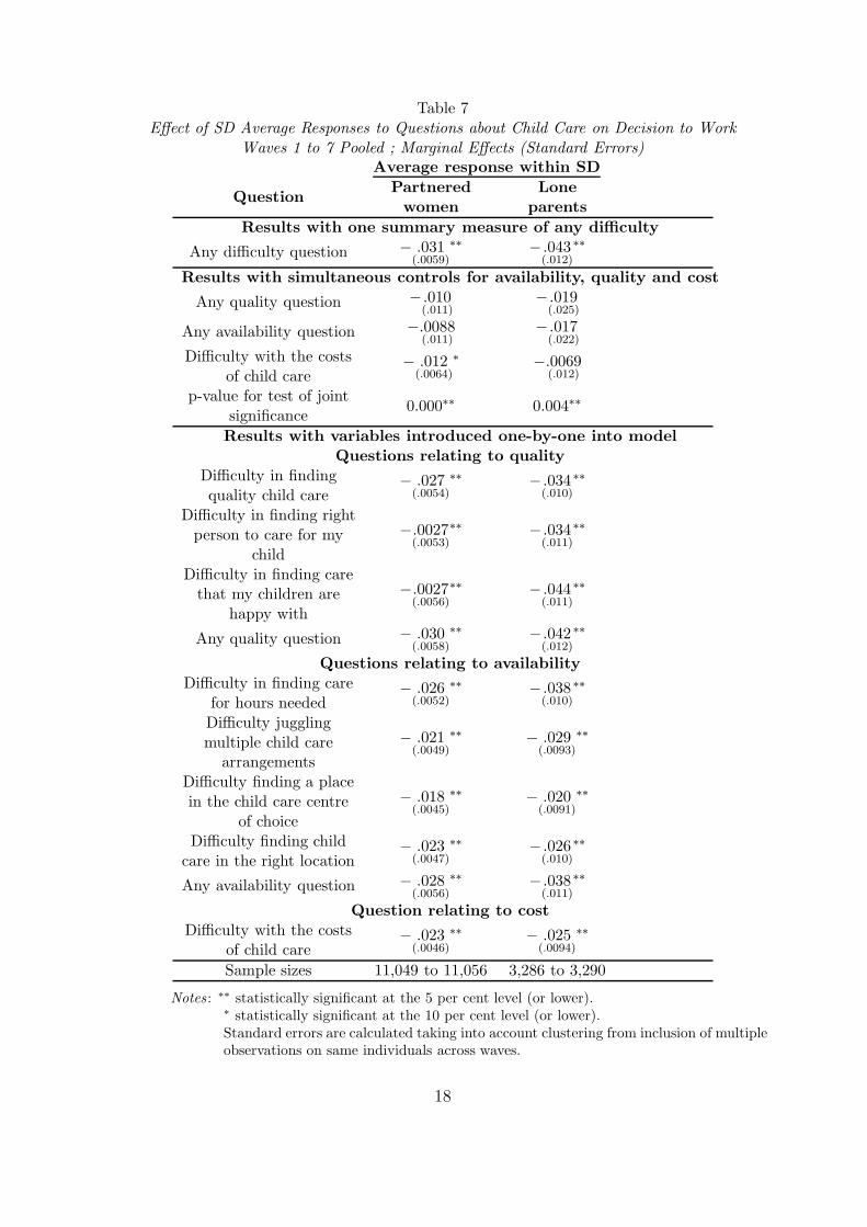
Table 7Effect of SD Average Responses to Questions about Child Care on Decision to Work
Waves 1 to 7 Pooled ; Marginal Effects (Standard Errors)Average response within SD
QuestionPartnered
womenLone
parentsResults with one summary measure of any difficulty
Any difficulty question − .031(.0059)
∗∗ − .043(.012)
∗∗
Results with simultaneous controls for availability, quality and cost
Any quality question − .010(.011)
− .019(.025)
Any availability question −.0088(.011)
− .017(.022)
Difficulty with the costsof child care
− .012(.0064)
∗ −.0069(.012)
p-value for test of jointsignificance
0.000∗∗ 0.004∗∗
Results with variables introduced one-by-one into modelQuestions relating to quality
Difficulty in findingquality child care
− .027(.0054)
∗∗ − .034(.010)
∗∗
Difficulty in finding rightperson to care for my
child
−.0027(.0053)
∗∗ − .034(.011)
∗∗
Difficulty in finding carethat my children are
happy with
−.0027(.0056)
∗∗ − .044(.011)
∗∗
Any quality question − .030(.0058)
∗∗ − .042(.012)
∗∗
Questions relating to availabilityDifficulty in finding care
for hours needed− .026
(.0052)
∗∗ − .038(.010)
∗∗
Difficulty jugglingmultiple child care
arrangements
− .021(.0049)
∗∗ − .029(.0093)
∗∗
Difficulty finding a placein the child care centre
of choice
− .018(.0045)
∗∗ − .020(.0091)
∗∗
Difficulty finding childcare in the right location
− .023(.0047)
∗∗ − .026(.010)
∗∗
Any availability question − .028(.0056)
∗∗ − .038(.011)
∗∗
Question relating to costDifficulty with the costs
of child care− .023
(.0046)
∗∗ − .025(.0094)
∗∗
Sample sizes 11,049 to 11,056 3,286 to 3,290
Notes : ∗∗ statistically significant at the 5 per cent level (or lower).∗ statistically significant at the 10 per cent level (or lower).Standard errors are calculated taking into account clustering from inclusion of multipleobservations on same individuals across waves.
18
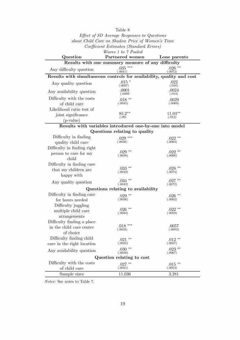
Table 8Effect of SD Average Responses to Questions
about Child Care on Shadow Price of Women’s TimeCoefficient Estimates (Standard Errors)
Waves 1 to 7 PooledQuestion Partnered women Lone parentsResults with one summary measure of any difficulty
Any difficulty question .035(.0041)
∗∗∗ .026(.0072)
∗∗
Results with simultaneous controls for availability, quality and cost
Any quality question .015(.0097)
∗ .022(.016)
Any availability question .0001(.0269
.0024(.014)
Difficulty with the costsof child care
.018(.0045)
∗∗ .0029(.0069)
Likelihood ratio test ofjoint significance
(p-value)
85.2(.00)
∗∗ 11.04(.012)
∗∗
Results with variables introduced one-by-one into modelQuestions relating to quality
Difficulty in findingquality child care
.029(.0038)
∗∗∗ .022(.0063)
∗∗
Difficulty in finding rightperson to care for my
child
.029(.0038)
∗∗ .022(.0066)
∗∗
Difficulty in finding carethat my children are
happy with
.033(.0043)
∗∗ .028(.0074)
∗∗
Any quality question .034(.0042)
∗∗ .027(.0072)
∗∗
Questions relating to availabilityDifficulty in finding care
for hours needed.029
(.0036)
∗∗ .026(.0062)
∗∗
Difficulty jugglingmultiple child care
arrangements
.026(.0034)
∗∗ .022(.0059)
∗∗
Difficulty finding a placein the child care centre
of choice
.018(.0032)
∗∗∗ .0057(.0052)
Difficulty finding childcare in the right location
.021(.0035)
∗∗ .012(.0057)
∗∗
Any availability question .030(.0039)
∗∗ .023(.0067)
∗∗
Question relating to costDifficulty with the costs
of child care.027
(.0031)
∗∗ .015(.0053)
∗∗
Sample sizes 11,036 3,281
Notes : See notes to Table 7.
19

To get some sense of the magnitude of these effects, consider the cost question. If
the level of reported difficulty with costs decreases by one (i.e. if average responses drop
from 3.93 to 2.93–a decrease of about 14
of a standard deviation), we can expect, for
partnered women, a 2.3 percentage point increase in the probability of working. The
effects are quite large for both partnered women and lone parents. Many households
already report zero problem with costs. What if only households who currently report
at least some difficulty with costs reduce their response by one unit? In this case, we
can expect a 1.6 percentage point increase in the probability of working.
(ii) Labour Supply
We augment the model of equation (1) with information about the quality/availability/cost
of child care in the same way as we did for the participation models of the previous sec-
tion. The model of equation (1) becomes
ln (wage∗i ) = α1 + α2hoursi + α3kidspreschooli + α4schoolkidsi + α5olderkidsi
+ α6nonreskidsi + α7homeowneri + α8wage pi + α10AV GSD,(−i) + ui (5)
where AV GSD,(−i) is the average response level (leaving out the ith person’s response)
in the SD for those cases where there are at least two responses to the question. The
wage equation (2) remains unchanged. For lone parents, the shadow wage equation, (3),
is transformed in similar fashion. If child care difficulties matter for labour supply, we
expect α10 to be positive, as difficulties with child care make going to work relatively
less attractive, equivalent to raising the reservation wage.
Results for partnered women and lone parents are presented in Table 8. Again,
we only present the coefficient estimates for the child care variables. The coefficient
estimates for the other variables, in all cases, are very similar to those reported in Table
6. For partnered women and for lone parents, the child care variables are positive and
significant in the structural labour supply model. Local difficulties with child care raise
the cost of working (reservation wage). The any difficulty question is significant at the
one per cent level. The three variables on availability, quality and cost, when included
simultaneously, are significant at the one per cent level.
The effects are statistically significant, but they are also large. For partnered women,
if average complaints about the cost of child care decrease by one, the model results imply
20

that the probability of working increases by 1.7 per cent (the predicted probability of
working, from the model, increases from 90.1 per cent to 91.7 per cent) and that hours
worked (for workers) will increase by 1.4 hours per week. Predicted hours for workers
increases from 24.3 to 25.7 (per week).17 If average complaints decrease by one only for
those who previously report some difficulty, we find a 1.1 percentage point increase in
the probability of working and 0.98 hours per week increase in hours of labour supplied.
The results are consistent across the two models, with the predicted change in par-
ticipation being slightly smaller in the structural model than in the reduced form model.
(iii) Robustness of Results
We estimated the participation and labour supply models with a wider set of explana-
tory variables including a squared term in age, household wealth variables, additional
educational categories, and public tenancy. These were all insignificant in the models
of Section IV and V and do not affect the results of Section V. We also estimated
the baseline model with dummy variables for the different states/territories and capital
city. None of these were significant. We did not include them in subsequent models.
This latter result does provide some assurance that results from the local averages of
responses to child care questions are not being driven simply by state or capital city
differences.
We re-estimated the models of Tables 7 and 8 using three alternative levels of aggre-
gation, 9-digit Statistical Local Area (SLA), 5-digit Labour Force Region (LFR), and
a combination of Major Statistical Region (MSR) and Section of State (SOS) informa-
tion.18 SLAs are quite small and for half of all SLAs we only have one response to the
child care questions forcing us to use only half the sample. Nonetheless, when we pool
across all seven waves, we find statistically significant effects of the child care variables
on participation and labour supply similar to what is reported here. Results for LFR
and MSR/SOS are very similar to what is reported here for SD. Our preferred level of
aggregation from a theoretical point of view is SD. SLA is clearly too small. People
seek and obtain work well outside of the SLA in which they live, but almost never out-
side of the SD in which they live (except for boundary cases.) There appears to be a
misconception that LFR is designed to capture the geographical area in which people
21

look for work. However, LFRs are chosen such that they have equal sample sizes and
with no reference to natural areas in which people live and work (and seek child care).19
A quick inspection of LFRs in the major cities around Australia show that they make
arbitrary divisions between neighbouring suburbs which are clearly in the same region
when it comes to commuting for work or choosing a school or a child care centre. The
main advantage of SDs is that they treat the main urban centres as a single unit. While
the SD is fairly wide and may include areas that are far from where a person lives,
they are usually within commuting distance and at least some people seek child care
close to work when they work far from home. Lastly, we believe that SD is the right
level of aggregation to capture local supply and demand forces which determine quality,
availability, and cost of child care.
We re-estimated all of the models of Tables 7 and 8 including the SDs where we only
have one response to the child care questions. In this case, we set the response equal
to zero for that individual (since when we use our leave-one-out calculation there are
zero observations) and we include a dummy variable equal to one if an observation is
in an SD with only one response to the child care questions. The results are virtually
unchanged and we can conclude that dropping these few observations does not have an
important impact on the outcomes.
VI Discussion and Conclusion
In this paper we show a significant statistical relationship between reports of difficulties,
aggregated at the local level, with child care–affordability, quality, and availability–and
the labour supply of partnered women and lone parents. Partnered women and lone
parents in areas which have higher average reports of problems with quality, availability
and cost work fewer hours and are less likely to work relative to their counterparts
in areas with lower average reports of child care difficulties. By using average reports
on subjective measures of difficulties with obtaining child care and excluding the own
individual’s response, we avoid the problem of correlation between an individual’s work
choices and her reported problems with child care.
Interestingly, reports of problems with availability, quality and cost are highly cor-
related and all of the questions appear to have a very strong common element to them.
22

We take this as evidence that people respond to these questions on the basis of overall
difficulty with obtaining child care and do not cleanly separate out quality from cost
from availability. This makes sense. Imagine a case where a person must choose from
a low-quality centre near home and a similarly-priced but high-quality centre far from
home. The problem could be expressed as one of quality, one of availability (the un-
availability of a high-quality centre near home), or one of cost (the additional expense
of commuting to the high-quality centre).
This paper was motivated by two concerns. The first is scepticism about the consen-
sus in the Australian literature that women’s labour supply is not very responsive to the
child care environment, particularly with respect to the price of child care. The second
concern is the lack of research on non-price factors of child care such as quality and
availability and the relationship of these non-price factors to labour supply decisions.
Our results, while exploratory in nature, lead us to question whether the consensus is
in fact correct and indicate that further research on non-price factors is likely to be
rewarding.
There are several caveats to our results. The first important caveat is that, since
the measures we use appear to indicate the overall difficulty in finding satisfactory child
care in a convenient location with a reasonable price, the measures do not allow us to
clearly separate the issues of child care availability, affordability and quality. Secondly,
we are unable to interpret these results with respect to specific policy initiatives which
might be considered.
However, an indirect implication can be derived using the estimates from Yamauchi
(2010). These indicate that an increase in the number of child care places per 100
children aged 0-4 from zero to the range of 15-25 is associated with a decline in the
measure indicating the difficulty in ‘finding good quality’ care by about one point, or
a 0.3 standard deviation. This estimate, coupled with our results on the structural
labour supply model, implies that, if some policy could induce an increase in child care
availability of this magnitude, our results imply that the probability of working will
increase by 1.8 percentage points and that the number of hours worked per week will
increase, on average, by 1.5.
Nonetheless, our results serve two important purposes in advancing the literature
23

on child care in Australia. Firstly, many of the studies mentioned in Section 2 above
find no significant effect on labour supply of child care price. Rammohan and Whelan
(2007), for example, find no significant effect on the propensity to work part-time in
response to higher child care prices. Doiron and Kalb (2005) find a very small elasticity
of work hours with respect to the price of child care among married mothers. These
studies have led to a consensus that labour supply is not very responsive to child care
affordability in Australia. Our paper would suggest that in fact there is something going
on between maternal labour supply choices and child care cost, availability and quality,
contradicting that consensus.
Secondly, this study shows that subjective evaluations of quality, availability and
cost are correlated with maternal labour supply. These descriptive results indicate that
future research based on accurate, objective measures of quality, availability, and cost
is likely to be fruitful in understanding the relationship between child care and labour
supply. Such research could be done with existing administrative data if it were made
available to researchers. Data about staff qualifications, length of waiting lists, physical
location and number of places would all provide more objective measures of quality and
availability. The child care census data, held by the Commonwealth Department of
Education, Employment and Workplace Relations has exactly the information that is
needed. This information, aggregated to an appropriate geographic level such as SD, and
matched to survey data would provide a powerful way to address very specific questions
about chid care availability, quality and cost and their relationship to people’s decisions
about working. Making use of the potential of this kind of detailed, administrative data
is in the interest of both academics and policy-makers as it would significantly help
improve our understanding of the relationship between child care and labour supply.
24

References
ABC (2009). Councils urge child care funding boost. Last accessed March 24, 2009.Available at http://www.abc.net.au/news/stories/2009/02/25/2500918.htm.
ABC Radio (2006). Childcare rebate to stay: Costello. Transcript available athttp://www.abc.net.au/worldtoday/content/2006/s1590212.htm. Last accessedMarch 20, 2009.
Anderson, P. M. and Levine, P. B. (1999). Child care and mothers’ employment de-cisions. NBER Working Paper No. W7058. Available at SSRN: http://ssrn.com/abstract=227421.
Australian Bureau of Statistics (2004). Labour force survey regions. Technical report,Australian Bureau of Statistics. Catalogue Number 6105.0 Available at http:
//www.abs.gov.au/AUSSTATS/[email protected]/94713ad445ff1425ca25682000192af2/
44a9700b59346b98ca256f5600768aac!OpenDocument. Last accessed on June 10,2009.
Australian Bureau of Statistics (2005). Australian Standard Geographical Classifica-tion (ASGC). Technical report, Australian Bureau of Statistics. Catalogue number1216.0. Available at http://www.abs.gov.au/AUSSTATS/[email protected]/lookup/1216.
0Contents12005. Last accessed on March 13, 2009.
Australian Human Rights Commission (2009). Get the facts–know your rights. fact sheet9: Returning to work. Last accessed March 24, 2009. Available at http://www.hreoc.gov.au/sex_discrimination/publication/get_the_facts/fact_sheet9.html.
Baker, M., Gruber, J., and Milligan, K. (2008). Universal childcare, maternal laborsupply and family well-being. Journal of Political Economy, 116(4):709–745.
Blau, D. M. (1991). The economics of child care. Russell Sage Foundation, New York,NY.
Blau, D. M. (2001). The child care problem: an economic analysis. Russell Sage Foun-dation, New York, NY.
Blau, D. M. and Currie, J. (2006). Pre-school, day care, and after-school care: Who’sminding the kids? In Hanushek, E. and Welch, F., editors, Handbook of the Economicsof Education, volume 2, chapter 20, pages 1163–1278. North-Holland.
Blau, D. M. and Hagy, A. P. (1998). The demand for quality in child care. Journal ofPolitical Economy, 106(1):104–146.
Blau, D. M. and Mocan, N. (2002). The supply of quality in child care centers. Reviewof Economics and Statistics, 84(3):483–496.
Breunig, R., Cobb-Clark, D., and Gong, X. (2008). Improving the modeling of couples’labour supply. Economic Record, 84(267):466–485.
25

Breunig, R. and Mercante, J. (2010). The accuracy of predicted wages of the non-employed and implications for policy simulations from structural labour supply mod-els. Economic Record, 86(272):49–70.
Cassells, R., McNamara, J., Lloyd, R., and Harding, A. (2005). Perceptions of childcare affordability and availability in Australia: what the HILDA survey tells us. Un-numbered NATSEM Working Paper. Canberra, Australia: National Centre for Socialand Economic Modeling.
Del Boca, D. and Vuri, D. (2007). The mismatch between employment and child carein Italy: the impact of rationing. Journal of Population Economics, 20(4):805–832.
Doiron, D. J. and Kalb, G. R. (2005). Demands for childcare and household laboursupply in Australia. Economic Record, 81(254):215–236.
Gustafsson, S. and Stafford, F. (1992). Child care subsidies and labor supply in Sweden.Journal of Human Resources, 27(1):204–230.
Hagy, A. P. (1998). The demand for child care quality: An hedonic price theory ap-proach. Journal of Human Resources, 33(3):683–710.
Heckman, J. J. (1974). Shadow prices, market wages and labor supply. Econometrica,42(4):679–694.
Hofferth, S. L. and Wissoker, D. A. (1992). Price, quality, and income in child carechoice. Journal of Human Resources, 27(1):70–111.
Kalb, G. R. (2002). Estimation of labour supply models for four separate groups in theAustralian population. Melbourne Institute Working Paper No. 24/02. Available athttp://melbourneinstitute.com/wp/wp2002n24.pdf.
Kalb, G. R. and Lee, W.-S. (2008). Childcare use and parents labour supply in Australia.Australian Economic Papers, 47(3):272–295.
Kornstad, T. and Thoresen, T. O. (2007). A discrete choice model for labour supplyand childcare. Journal of Population Economics, 20:781–803.
Lehrer, E. L. (1989). Preschoolers with working mothers: an analysis of the determinantsof child care arrangements. Journal of Population Economics, 1:251–268.
Leibowitz, A., Waite, L. J., and Witsberger, C. (1988). Child care for preschoolers:differences by child’s age. Demography, 25:205–220.
Lokshin, M. (2004). Household childcare choices and women’s work behavior in russia.The Journal of Human Resources, 39(4):1094–1115.
Mocan, N. (2007). Can consumers detect lemons? an empirical analysis of informationasymmetry in the market for child care. Journal of Population Economics, 20(4):743–780.
26

Rammohan, A. and Whelan, S. (2005). Child care and female employment decisions.Australian Journal of Labour Economics, 8(2):203–225.
Rammohan, A. and Whelan, S. (2007). The impact of childcare costs on the full-time/part-time employment decisions of australian mothers. Australian EconomicPapers, 46(2):152–169.
The Parliament of the Commonwealth of Australia (2006). Balancing work and family:Report on the inquiry into balancing work and family. Technical report, Common-wealth of Australia. Canberra, Australia.
Van Soest, A. (1995). Structural models of family labour supply–a discrete choiceapproach. The Journal of Human Resources, 30:63–88.
Watson, N. and Wooden, M. (2002). The Household, Income and Labour Dynamics inAustralia (HILDA) survey: wave 1 survey methodology. Technical report. HILDAProject Technical Paper Series, No. 1/02.
Wrohlich, K. (2006). Labor supply and child care choices in a rationed child care market.IZA Discussion Paper number 2053.
Yamauchi, C. (2010). The availability of child care centers and parental perceivedaccessibility and life satisfaction. Review of Economics of the Household, 8(2):231–253.
27

Appendix
Table A1: Correlation between Individual-level Responses to Child Care Difficulty Questions:HILDA Respondents with Children Under age 15 who used or Considered using Child Care
Waves 1 Through 7 Pooled
qual1 qual2 qual3 avail1 avail2 avail3 avail4 cost1 anyqual anyavailqual2 0.82qual3 0.68 0.68avail1 0.70 0.70 0.57avail2 0.49 0.50 0.51 0.55avail3 0.71 0.62 0.62 0.61 0.48avail4 0.68 0.61 0.63 0.58 0.47 0.81cost1 0.45 0.46 0.44 0.45 0.50 0.41 0.39anyqual 0.92 0.93 0.87 0.73 0.55 0.72 0.71 0.50anyavail 0.77 0.73 0.69 0.85 0.77 0.89 0.87 0.52 0.81anydiff 0.87 0.86 0.81 0.82 0.72 0.84 0.82 0.66 0.93 0.94
Table A2: Correlation between SD-level Average Responses to Child Care DifficultyQuestions: HILDA Respondents with Children Under age 15 who used or Considered using
Child CareWaves 1 Through 7 Pooled
qual1 qual2 qual3 avail1 avail2 avail3 avail4 cost1 anyqual anyavailqual2 0.79qual3 0.68 0.69avail1 0.76 0.70 0.63avail2 0.31 0.43 0.45 0.44avail3 0.68 0.54 0.52 0.62 0.26avail4 0.59 0.55 0.50 0.58 0.27 0.78cost1 0.46 0.49 0.49 0.43 0.39 0.37 0.29anyqual 0.92 0.90 0.87 0.78 0.43 0.66 0.61 0.54anyavail 0.78 0.70 0.67 0.87 0.54 0.84 0.81 0.47 0.81anydiff 0.88 0.84 0.81 0.86 0.53 0.78 0.73 0.63 0.94 0.94
28

Notes
∗ Corresponding author: Robert Breunig, Research School of Economics, Australian
National University, Canberra, ACT 0200 Australia; E-mail: [email protected].
Robert Breunig would like to thank the Australian Treasury for their support and hospi-
tality. This paper has been improved by comments from Paul Miller and an anonymous
referee. We appreciate comments from seminar participants at the LaTrobe Univer-
sity, Paris I Sorbonne, and the OECD. This paper uses in-confidence unit record data
from the Household, Income and Labour Dynamics in Australia (HILDA) survey. The
HILDA project was initiated and is funded by the Commonwealth Department of Fam-
ilies, Housing, Community Services and Indigenous Affairs (FaHCSIA) and managed
by the Melbourne Institute of Applied Economic and Social Research (MIAESR). The
findings and views reported in this paper, however, are those of the authors and the
views should not be attributed to FaHCSIA, MIAESR or the Australian Treasury.
1The Australian Broadcasting Corporation (ABC) is unrelated to ABC learning.
2We estimate separate models for partnered women and lone parents. This follows
most Australian studies which estimate labour supply separately for partnered women,
partnered men, lone parents, and singles. We include partnered women without children
in the model for comparability with other studies (e.g. Kalb, 2002; Breunig et al., 2008)
of partnered women’s labour supply. We assume that labour supply of women without
children is unaffected by local child care supply conditions.
3We are grateful to a referee for pointing out that part of the explanation in Australia
may be related to the very low cost per hour of child care which is found in datasets
such as HILDA–see Rammohan and Whelan (2007).
4A recent example is Baker et al. (2008) for Canada. Anderson and Levine (1999)
and Blau and Currie (2006) review the international literature.
5See Watson and Wooden (2002) for more details.
29
6Wages of these individuals are well below the average wage for partnered women and
are probably the result of positive measurement error in hours. This measurement error
induces a negative correlation in observed hours and wages (because the measurement
error affects hours positively and wages negatively) and such extreme observations can
introduce large bias into our labour supply estimates.
7Details of wave-by-wave exclusions are available from the authors.
8Wave-by-wave versions of Tables 1 through 4 are available upon request from the
authors.
9Specifically, these questions relate to ‘care for a sick child’, ‘care during the school
holidays’, ‘care for a difficult or special needs child’, ‘care at short notice’. For families
for whom these concerns are not relevant, it is unclear how they would form their opinion
about these types of care.
10We use all household responses to these questions, pooling across all household
types. These responses include households which are neither in our analysis sample for
partnered women nor for lone parents. For example, couple-headed households where
data for the partnered female is missing would not be included in our analysis sample
but could be included in our aggregate child care data if responses to these questions
were provided on the household form.
11See Cassells et al. (2005) for a detailed, and very informative, descriptive study of
the HILDA child care data.
12SD are described in Australian Bureau of Statistics (2005).
13The household correlations are documented in Appendix Table A1 and the correla-
tions within SD are presented in Appendix Table A2.
14Partnered women who are defined as “not in the labour force” transition to em-
ployment at fairly high rates, but only about half as much as partnered women who are
defined as “unemployed”. They also tend to take up employment at higher wages than
the unemployed, so there appears to be something fundamentally different about their
30

non-employed status. See Breunig and Mercante (2010) who document these facts for
this data set.
15This represents a 1.5 to 2 per cent increase in hours, which is fairly large. The
Heckman (1974) model, which assumes that hours freely adjust so that wage = wage∗
for workers (see equations (1) and (2), tends to produce fairly large estimates of labour
supply elasticities. Models which restrict working hours to commonly observed discrete
points (for Australia, see Breunig et al., 2008) tend to produce smaller labour supply
elasticities.
16We drop the individual who responded to the child care question and also any other
observations in the SD. This latter group includes households who do not use child
care and who did not respond to the child care questions. Excluding some observations
from an SD on the basis of whether or not households used child care would introduce
selection, so it is cleaner to simply drop all observations from these SDs. This involves
dropping at most (depending upon the question) 11 out of 3,297 observations from
the lone parent sample and dropping at most 54 out of 11,103 observations from the
partnered women sample. We report on what happens if we include these observations
in Section V(iii) below.
17These changes are calculated numerically from the model estimates.
18See Australian Bureau of Statistics (2005) for definitions of these local regions.
These results are available in a detailed working paper available at http://econrsss.
anu.edu.au/Staff/breunig/workpapers_bb.htm.
19Australian Bureau of Statistics (2004) documents how LFRs are chosen.
31