Chetty - Public Economics Lectures
951
Public Economics Lectures Part 1: Introduction Raj Chetty and Gregory A. Bruich Harvard University Fall 2009 Public Economics Lectures () Part 1: Introduction 1 / 28
-
Upload
madminarch -
Category
Documents
-
view
237 -
download
0
Transcript of Chetty - Public Economics Lectures

8/8/2019 Chetty - Public Economics Lectures
http://slidepdf.com/reader/full/chetty-public-economics-lectures 1/949
Public Economics LecturesPart 1: Introduction
Raj Chetty and Gregory A. Bruich
Harvard University
Fall 2009
Public Economics Lectures ()
Part 1: Introduction 1 / 28

8/8/2019 Chetty - Public Economics Lectures
http://slidepdf.com/reader/full/chetty-public-economics-lectures 2/949
What is Public Economics?
Public economics focuses on answering two types of questions
1 How do government policies a¤ect the economy?
2 How should policies be designed to maximize welfare?
Three motivations for studying these questions:
1 Practical Relevance
2 Academic Interest
3 Methodology
Public Economics Lectures ()
Part 1: Introduction 2 / 28

8/8/2019 Chetty - Public Economics Lectures
http://slidepdf.com/reader/full/chetty-public-economics-lectures 3/949
Motivation 1: Practical Relevance
Interest in improving economic welfare ! interest in public economics
Almost every economic intervention occurs through governmentpolicy (i.e. involves public economics) via two channels:
Price intervention: taxes, welfare, social insurance, public goods
Regulation: min wages, FDA regulations (25% of products consumed),zoning laws, labor laws, min education laws, environment, legal code
Government directly employs one sixth of U.S. workforce
Public Economics Lectures ()
Part 1: Introduction 3 / 28

8/8/2019 Chetty - Public Economics Lectures
http://slidepdf.com/reader/full/chetty-public-economics-lectures 4/949
Motivation 1: Practical Relevance
Stakes are extremely large because of broad scope of policies
Ex. Tax reforms immediately a¤ect millions
Contentious debate on the appropriate role of government in society
Controversial: liberals vs. conservatives
McCain: “Obama proposes higher taxes. Therefore 5M fewer jobs”
Obama: “Alternative energy investment will create 5M U.S. jobs”
Which view is right? Injecting science into these political debates hastremendous practical value
Public Economics Lectures () Part 1: Introduction 4 / 28

8/8/2019 Chetty - Public Economics Lectures
http://slidepdf.com/reader/full/chetty-public-economics-lectures 5/949
Motivation 2: Academic Interest
Public economics is typically the end point for many other sub…elds of
economics
Macro, development, labor, and corporate …nance questions oftenultimately motivated by a public economics issue
Ex 1: Macro studies on costs of business cycles and intertemporalmodels of household behavior
Ex 2: Labor studies on employment e¤ects of the minimum wage
Natural to combine public …nance with another …eld
Understanding public …nance can help sharpen your research focusand ensures you are working on relevant issues
Public Economics Lectures () Part 1: Introduction 5 / 28

8/8/2019 Chetty - Public Economics Lectures
http://slidepdf.com/reader/full/chetty-public-economics-lectures 6/949
Motivation 3: Methodology
Modern public economics tightly integrates theory with empiricalevidence to derive quantitative predictions about policy
What is the optimal income tax rate?
What is the optimal unemployment bene…t level?
Combining applied theory and evidence is a useful skill set that is at
the frontier of many …elds of economics
Public Economics Lectures () Part 1: Introduction 6 / 28

8/8/2019 Chetty - Public Economics Lectures
http://slidepdf.com/reader/full/chetty-public-economics-lectures 7/949
Methodological Themes
1 Micro-based empirics but both micro and macro theory
2 Two styles of work: structural and reduced-form
3 Neoclassical, but growing interest in implications of behavioral econfor public policy
4 Focus primarily on developed countries because of data availability,but growing interest in developing countries
5 Long run focus in theory: focus on ideal design of systems for longrun welfare but short-run focus in empirics
6 Two approaches to research: bringing in new ideas from other …eldsvs. innovating within public economics
Public Economics Lectures () Part 1: Introduction 7 / 28

8/8/2019 Chetty - Public Economics Lectures
http://slidepdf.com/reader/full/chetty-public-economics-lectures 8/949
Background Facts: Size and Growth of Government
Government expenditures = 1/3 GDP in the U.S.
Higher than 50% of GDP in some European countries
Decentralization is a key feature of U.S. govt
One third of spending (10% of GDP) is done at state-local level (e.g.schools)
Two thirds (20% of GDP) is federal
Public Economics Lectures () Part 1: Introduction 8 / 28

8/8/2019 Chetty - Public Economics Lectures
http://slidepdf.com/reader/full/chetty-public-economics-lectures 9/949
0
1 0
2
0
3 0
4 0
5 0
R e v e n u e a n d
s p e n d i n g ( % o
f G D P )
1930 1940 1950 1960 1970 1980 1990 2000 2010
Year
Revenue Expenditure
Federal Government Revenue and Expenditure 1930-2009
Source: Office of Management and Budget, Historical Tables, FY 2011
Public Economics Lectures () Part 1: Introduction 9 / 28
8/8/2019 Chetty - Public Economics Lectures
http://slidepdf.com/reader/full/chetty-public-economics-lectures 10/949
2 0
3 0
4 0
5 0
6 0
1970 1975 1980 1985 1990 1995 2000 2005
Sweden
Canada
United States
OECD Avg. P e r c e n t o f G D P
Year
Total Government Spending by Country, 1970-2007
Source: OECD Economic Outlook (2009)
Public Economics Lectures () Part 1: Introduction 10 / 28
8/8/2019 Chetty - Public Economics Lectures
http://slidepdf.com/reader/full/chetty-public-economics-lectures 11/949
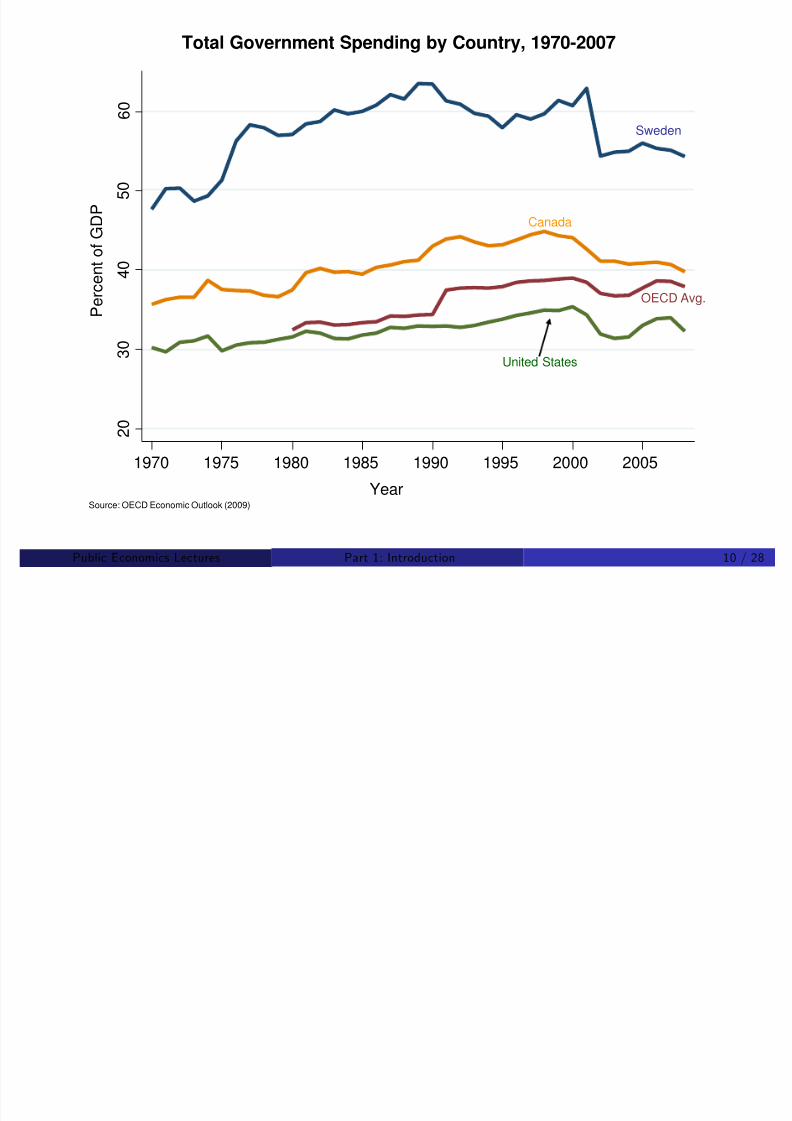
Federal Revenues (% of total revenue)
1960
Excise
2.7%Other 4.2%
Other4.2%
2008
Source: Office of Management and Budget, historical tables, government receipts by source
Income
44% Payroll15.9%
Corporate23.2%
Excise12.6%
Income
44% Payroll15.9%
Corporate23.2%
Excise12.6%
Income
45.4%
Corporate
12.1%
Payroll37.5%
Income
45.4%
Corporate
12.1%
Payroll37.5%
Public Economics Lectures () Part 1: Introduction 11 / 28

8/8/2019 Chetty - Public Economics Lectures
http://slidepdf.com/reader/full/chetty-public-economics-lectures 12/949
State/Local Revenues (% of total revenue)
Federal Grants9.4%
Income Tax5.9%
1960 2007
Source: U.S. Census Bureau, 2007 Summary of State & Local Government
PropertyTax
38.2%
Sales Tax28.8%
Other
17.7%
PropertyTax
38.2%
Sales Tax28.8%
Other
17.7%
PropertyTax 15.7%
Sales Tax17.9%
Other
33%
Federal
Grants19.1%
Income Tax14.3%
PropertyTax 15.7%
Sales Tax17.9%
Other
33%
Federal
Grants19.1%
Income Tax14.3%
Public Economics Lectures () Part 1: Introduction 12 / 28

8/8/2019 Chetty - Public Economics Lectures
http://slidepdf.com/reader/full/chetty-public-economics-lectures 13/949
Federal Spending (% of total spending)
1960 2001
Source: Office of Management and Budget, historical tables, government outlays by function
Health, 2.9%
Other
12.4%
Net Interest
8.3%UI and
Disability
8.9%
Social
Security
13.5%
Education, welfare, housing 4%
UI and Disability, 6.3%
Other
11.2%
Health23.1%
Net
Interest
12.3%
Social
Security19.5%
Other
11.2%
Health23.1%
Net
Interest
12.3%
Social
Security19.5%
Education, welfare, housing 9.7%
Public Economics Lectures () Part 1: Introduction 13 / 28

8/8/2019 Chetty - Public Economics Lectures
http://slidepdf.com/reader/full/chetty-public-economics-lectures 14/949
Payroll
24.3%
Wealth,2.2%
Consumption73.5%
Mexico
Payroll
20.5%
IndividualIncome24.2%
Wealth, 2.2%
Consumption31.3%
Norway
CorporateIncome 21.7%
Payroll
20.5%
IndividualIncome24.2%
Wealth, 2.2%
Consumption31.3%
Norway
CorporateIncome 21.7%
OECD Average
Payroll26.7%
IndividualIncome
26%
Corporate Income, 9.3%
Wealth, 5.5%
Consumption32.6%
OECD Average
Payroll26.7%
IndividualIncome
26%
Corporate Income, 9.3%
Wealth, 5.5%
Consumption32.6%
International Tax Revenue by Type of Tax (2001, % of Total)
Source: OECD 2002
Public Economics Lectures () Part 1: Introduction 14 / 28

8/8/2019 Chetty - Public Economics Lectures
http://slidepdf.com/reader/full/chetty-public-economics-lectures 15/949
Government Intervention in the Economy
Organzing framework: “When is government intervention necessary ina market economy?”
Market …rst, govt. second approach
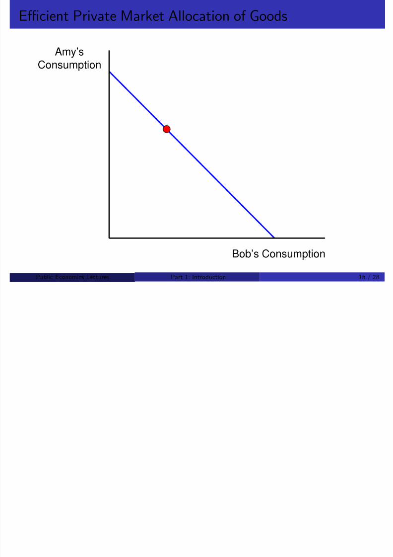
Why? Private market outcome is e¢cient under broad set of conditions(1st Welfare Thm)
Course can be split into two parts:
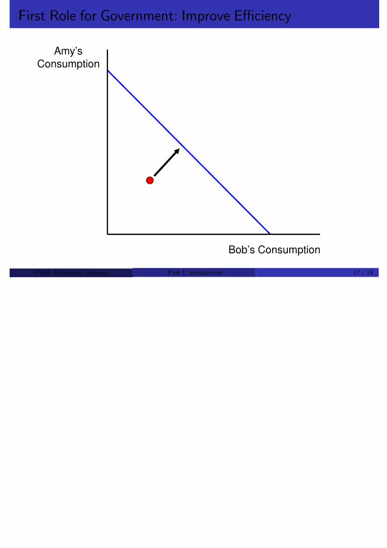
1 How can govt. improve e¢ciency when private market is ine¢cient?
2 What can govt. do if private market outcome is undesirable due toredistributional concerns?
Public Economics Lectures () Part 1: Introduction 15 / 28
8/8/2019 Chetty - Public Economics Lectures
http://slidepdf.com/reader/full/chetty-public-economics-lectures 16/949
E¢cient Private Market Allocation of Goods
Amy’s
Consumption
Bob’s Consumption
Public Economics Lectures () Part 1: Introduction 16 / 28
Fi R l f G I E¢ i
8/8/2019 Chetty - Public Economics Lectures
http://slidepdf.com/reader/full/chetty-public-economics-lectures 17/949
First Role for Government: Improve E¢ciency
Amy’s
Consumption
Bob’s Consumption
Public Economics Lectures () Part 1: Introduction 17 / 28
S d R l f G I Di ib i

8/8/2019 Chetty - Public Economics Lectures
http://slidepdf.com/reader/full/chetty-public-economics-lectures 18/949
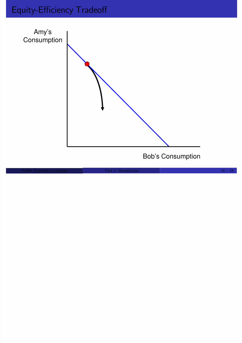
Second Role for Government: Improve Distribution
Amy’s
Consumption
Bob’s Consumption
Public Economics Lectures () Part 1: Introduction 18 / 28
Fi W lf Th
8/8/2019 Chetty - Public Economics Lectures
http://slidepdf.com/reader/full/chetty-public-economics-lectures 19/949
First Welfare Theorem
Private market provides a Pareto e¢cient outcome under threeconditions
1 No externalities
2 Perfect information
3 Perfect competition
Theorem tells us when the government should intervene
Public Economics Lectures () Part 1: Introduction 19 / 28
F il 1 E t liti

8/8/2019 Chetty - Public Economics Lectures
http://slidepdf.com/reader/full/chetty-public-economics-lectures 20/949
Failure 1: Externalities
Markets may be incomplete due to lack of prices (e.g. pollution)
Achieving e¢cient Coasian solution requires an organization tocoordinate individuals – that is, a government
This is why govt. funds public goods (highways, education, defense)
Questions: What public goods to provide and how to correct
externalities?
Public Economics Lectures () Part 1: Introduction 20 / 28
F il 2 A t i I f ti d I l t M k t

8/8/2019 Chetty - Public Economics Lectures
http://slidepdf.com/reader/full/chetty-public-economics-lectures 21/949
Failure 2: Asymmetric Information and Incomplete Markets
When some agents have more information than others, markets fail
Ex. 1: Adverse selection in health insurance
Healthy people drop out of private market ! unraveling
Mandated coverage could make everyone better o¤
Ex. 2: capital markets (credit constraints) and subsidies for education
Ex. 3: Markets for intergenerational goods
Future generations’ interests may not be fully re‡ected in marketoutcomes
Public Economics Lectures () Part 1: Introduction 21 / 28
Failure 3: Imperfect Competition

8/8/2019 Chetty - Public Economics Lectures
http://slidepdf.com/reader/full/chetty-public-economics-lectures 22/949
Failure 3: Imperfect Competition
When markets are not competitive, there is role for govt. regulation
Ex: natural monopolies such as electricity and telephones
This topic is traditionally left to courses on industrial organizationand is not covered in this course
But taking the methodological approach of public economics to
problems traditionally analyzed in IO is a very promising area
Public Economics Lectures () Part 1: Introduction 22 / 28
Individual Failures

8/8/2019 Chetty - Public Economics Lectures
http://slidepdf.com/reader/full/chetty-public-economics-lectures 23/949
Individual Failures
Recent addition to the list of potential failures that motivate
government intervention: people are not fully rational
Government intervention (e.g. by forcing saving via social security)may be desirable
This is an “individual” failure rather than a traditional market failure
Conceptual challenge: how to avoid paternalism critique
Why does govt. know better what’s desirable for you (e.g. wearing aseatbelt, not smoking, saving more)
Di¢cult but central issues to policy design
Public Economics Lectures () Part 1: Introduction 23 / 28
Redistributional Concerns
8/8/2019 Chetty - Public Economics Lectures
http://slidepdf.com/reader/full/chetty-public-economics-lectures 24/949
Redistributional Concerns
Even when the private market outcome is e¢cient, may not havegood distributional properties
E¢cient markets generally seem to deliver very large rewards to smallset of people (top incomes)
Government can intervene to redistribute income through tax andtransfer system
Public Economics Lectures () Part 1: Introduction 24 / 28
Why Limit Government Intervention?

8/8/2019 Chetty - Public Economics Lectures
http://slidepdf.com/reader/full/chetty-public-economics-lectures 25/949
Why Limit Government Intervention?
One solution to these issues would be for the government to overseeall production and allocation in the economy (socialism).
Serious problems with this solution
1 Information: how does government aggregate preferences andtechnology to choose optimal production and allocation?
2 Government policies inherently distort incentives (behavioral responsesin private sector)
3 Politicians not necessarily a benevolent planner in reality; face incentiveconstraints themselves
Creates sharp tradeo¤s between costs and bene…ts of government
intervention
Providing more public goods requires higher taxes and distortsconsumption decisions
Redistribution distorts incentives to workPublic Economics Lectures () Part 1: Introduction 25 / 28
8/8/2019 Chetty - Public Economics Lectures
http://slidepdf.com/reader/full/chetty-public-economics-lectures 26/949
Three Types of Questions in Public Economics

8/8/2019 Chetty - Public Economics Lectures
http://slidepdf.com/reader/full/chetty-public-economics-lectures 27/949
Three Types of Questions in Public Economics
1
Positive analysis: What are the observed e¤ects of governmentprograms and interventions?
2 Normative analysis: What should the government do if we can chooseoptimal policy?
3 Public choice/Political Economy
Develops theories to explain why the government behaves the way itdoes and identify optimal policy given political economy concerns
Criticism of normative analysis: fails to take political constraints intoaccount
Public Economics Lectures () Part 1: Introduction 27 / 28
Course Outline

8/8/2019 Chetty - Public Economics Lectures
http://slidepdf.com/reader/full/chetty-public-economics-lectures 28/949
Course Outline
1 Tax Incidence and E¢ciency
2 Optimal Taxation
3 Income Taxation and Labor Supply
4 Social Insurance
5 Public Goods and Externalities
Public Economics Lectures () Part 1: Introduction 28 / 28
8/8/2019 Chetty - Public Economics Lectures
http://slidepdf.com/reader/full/chetty-public-economics-lectures 29/949
Public Economics LecturesPart 2: Incidence of Taxation
Raj Chetty and Gregory A. Bruich
Harvard UniversityFall 2009
Public Econom ics Lectures () Part 2: Tax Incidence 1 / 141

8/8/2019 Chetty - Public Economics Lectures
http://slidepdf.com/reader/full/chetty-public-economics-lectures 30/949
References on Tax Incidence

8/8/2019 Chetty - Public Economics Lectures
http://slidepdf.com/reader/full/chetty-public-economics-lectures 31/949
References on Tax Incidence
Kotliko¤ and Summers (1987) handbook chapter
Atkinson and Stiglitz text chapters 6 and 7
Chetty, Looney, and Kroft (2009)
Public Econom ics Lectures () Part 2: Tax Incidence 3 / 141
De…nition

8/8/2019 Chetty - Public Economics Lectures
http://slidepdf.com/reader/full/chetty-public-economics-lectures 32/949
Tax incidence is the study of the e¤ects of tax policies on prices andthe distribution of utilities
What happens to market prices when a tax is introduced or changed?
Increase tax on cigarettes by $1 per pack
Introduction of Earned Income Tax Credit (EITC)
Food stamps program
E¤ect on price ! distributional e¤ects on smokers, pro…ts of producers, shareholders, farmers, ...
Public Econom ics Lectures () Part 2: Tax Incidence 4 / 141
Economic vs. Statutory Incidence

8/8/2019 Chetty - Public Economics Lectures
http://slidepdf.com/reader/full/chetty-public-economics-lectures 33/949
y
Equivalent when prices are constant but not in general
Consider the following argument:
Government should tax capital income b/c it is concentrated at thehigh end of the income distribution
Neglects general equilibrium price e¤ects
Tax might be shifted onto workers
If capital taxes ! less savings and capital ‡ight, then capital stockmay decline, driving return to capital up and wages down
Some argue that capital taxes are paid by workers and thereforeincrease income inequality (Hassett and Mathur 2009)
Public Econom ics Lectures () Part 2: Tax Incidence 5 / 141
Overview of Literature

8/8/2019 Chetty - Public Economics Lectures
http://slidepdf.com/reader/full/chetty-public-economics-lectures 34/949
Tax incidence is an example of positive analysis
Typically the …rst step in policy evaluation
An input into thinking about policies that maximize social welfare
Theory is informative about signs and comparative statics but isinconclusive about magnitudes
Incidence of cigarette tax: elasticity of demand w.r.t. price is crucial
Labor vs. capital taxation: mobility of labor, capital are critical
Public Econom ics Lectures () Part 2: Tax Incidence 6 / 141
Overview of Literature

8/8/2019 Chetty - Public Economics Lectures
http://slidepdf.com/reader/full/chetty-public-economics-lectures 35/949
Ideally, we would characterize the e¤ect of a tax change on utilitylevels of all agents in the economy
Useful simpli…cation in practice: aggregate economic agents into afew groups
Incidence analyzed at a number of levels:
1 Producer vs. consumer (tax on cigarettes)2 Source of income (labor vs. capital)3 Income level (rich vs. poor)4 Region or country (local property taxes)5 Across generations (social Security reform)
Public Econom ics Lectures () Part 2: Tax Incidence 7 / 141

8/8/2019 Chetty - Public Economics Lectures
http://slidepdf.com/reader/full/chetty-public-economics-lectures 36/949

8/8/2019 Chetty - Public Economics Lectures
http://slidepdf.com/reader/full/chetty-public-economics-lectures 37/949
Partial Equilibrium Model: Demand

8/8/2019 Chetty - Public Economics Lectures
http://slidepdf.com/reader/full/chetty-public-economics-lectures 38/949
Consumer has wealth Z and has utility u (x , y )
Let εD = ∂D ∂p
q D (p )
denote the price elasticity of demand
Elasticity: % change in quantity when price changes by 1%
Widely used concept because elasticities are unit free
Public Econom ics Lectures () Part 2: Tax Incidence 10 / 141

8/8/2019 Chetty - Public Economics Lectures
http://slidepdf.com/reader/full/chetty-public-economics-lectures 39/949
Partial Equilibrium Model: Equilibrium

8/8/2019 Chetty - Public Economics Lectures
http://slidepdf.com/reader/full/chetty-public-economics-lectures 40/949
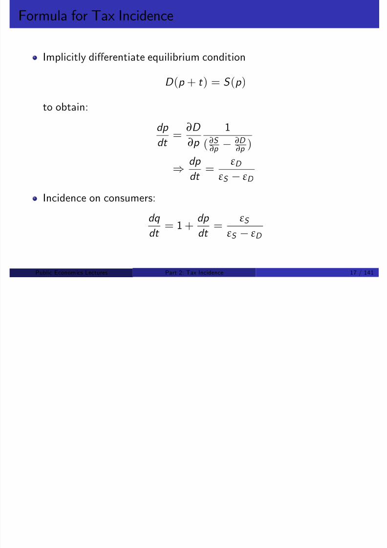
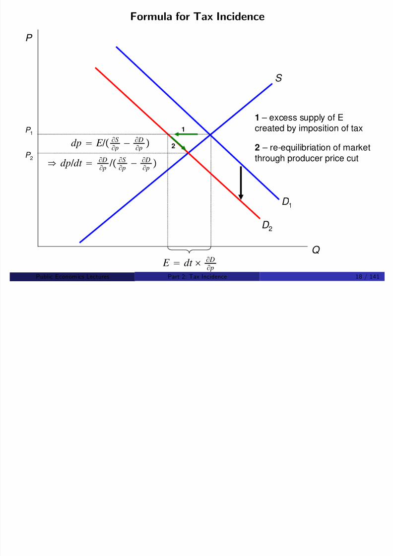
Equilibrium condition
Q = S (p ) = D (p + t )
de…nes an equation p (t )
Goal: characterize dp dt
, the e¤ect of a tax increase on price
First consider some graphical examples to build intuition, then
analytically derive formula
Public Econom ics Lectures () Part 2: Tax Incidence 12 / 141
Tax Levied on Producers

8/8/2019 Chetty - Public Economics Lectures
http://slidepdf.com/reader/full/chetty-public-economics-lectures 41/949
ConsumerBurden = $4.50
D
S
B
SupplierBurden = $3.00
Price
Quantity
$22.5$22.5
$19.5
$27.0
A
1250 1500
S+t
$7.50
$30.0
C
D
Public Econom ics Lectures () Part 2: Tax Incidence 13 / 141
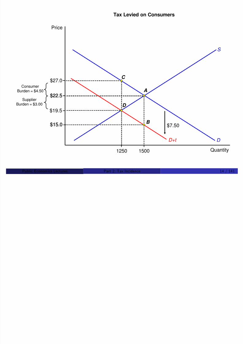
Tax Levied on Consumers
8/8/2019 Chetty - Public Economics Lectures
http://slidepdf.com/reader/full/chetty-public-economics-lectures 42/949
D
S
B
Price
Quantity
$22.5$22.5
$19.5
D+t
$7.50
$27.0
$15.0$15.0
A
1250 1500
D
C
ConsumerBurden = $4.50
SupplierBurden = $3.00
Public Econom ics Lectures () Part 2: Tax Incidence 14 / 141

8/8/2019 Chetty - Public Economics Lectures
http://slidepdf.com/reader/full/chetty-public-economics-lectures 43/949
Perfectly Elastic Demand

8/8/2019 Chetty - Public Economics Lectures
http://slidepdf.com/reader/full/chetty-public-economics-lectures 44/949
S S+t
Quantity
Price
D
$7.50
Supplierburden
1500
$22.5
$15.0
Public Econom ics Lectures () Part 2: Tax Incidence 16 / 141
8/8/2019 Chetty - Public Economics Lectures
http://slidepdf.com/reader/full/chetty-public-economics-lectures 45/949
8/8/2019 Chetty - Public Economics Lectures
http://slidepdf.com/reader/full/chetty-public-economics-lectures 46/949

8/8/2019 Chetty - Public Economics Lectures
http://slidepdf.com/reader/full/chetty-public-economics-lectures 47/949
8/8/2019 Chetty - Public Economics Lectures
http://slidepdf.com/reader/full/chetty-public-economics-lectures 48/949

8/8/2019 Chetty - Public Economics Lectures
http://slidepdf.com/reader/full/chetty-public-economics-lectures 49/949
Chetty et al.: Two Empirical Strategies

8/8/2019 Chetty - Public Economics Lectures
http://slidepdf.com/reader/full/chetty-public-economics-lectures 50/949
Two strategies to estimate θ:
1 Manipulate tax salience: make sales tax as visible as pre-tax price
E¤ect of intervention on demand:
v = log x ((1 + τ )p , 0) log x (p , τ )
Compare to e¤ect of equivalent price increase to estimate θ:
(1 θ) = v
εx ,p log(1 + τ )
2 Manipulate tax rate: compare εx ,p and εx ,1+τ
θ = εx ,1+τ /εx ,p
Public Econom ics Lectures () Part 2: Tax Incidence 22 / 141
Chetty et al.: Strategy 1

8/8/2019 Chetty - Public Economics Lectures
http://slidepdf.com/reader/full/chetty-public-economics-lectures 51/949
Experiment manipulating salience of sales tax implemented at asupermarket that belongs to a major grocery chain
30% of products sold in store are subject to sales tax
Posted tax-inclusive prices on shelf for subset of products subject tosales tax (7.375% in this city)
Data: Scanner data on price and weekly quantity sold by product
Public Econom ics Lectures () Part 2: Tax Incidence 23 / 141

8/8/2019 Chetty - Public Economics Lectures
http://slidepdf.com/reader/full/chetty-public-economics-lectures 52/949

8/8/2019 Chetty - Public Economics Lectures
http://slidepdf.com/reader/full/chetty-public-economics-lectures 53/949
Chetty et al.: Research Design

8/8/2019 Chetty - Public Economics Lectures
http://slidepdf.com/reader/full/chetty-public-economics-lectures 54/949
Quasi-experimental di¤erence-in-di¤erences
Treatment group:
Products : Cosmetics, Deodorants, and Hair Care Accessories
Store : One large store in Northern California
Time period : 3 weeks (February 22, 2006 – March 15, 2006)
Control groups:
Products : Other prods. in same aisle (toothpaste, skin care, shave)
Stores : Two nearby stores similar in demographic characteristics
Time period : Calendar year 2005 and …rst 6 weeks of 2006
Public Econom ics Lectures () Part 2: Tax Incidence 26 / 141

8/8/2019 Chetty - Public Economics Lectures
http://slidepdf.com/reader/full/chetty-public-economics-lectures 55/949

8/8/2019 Chetty - Public Economics Lectures
http://slidepdf.com/reader/full/chetty-public-economics-lectures 56/949
8/8/2019 Chetty - Public Economics Lectures
http://slidepdf.com/reader/full/chetty-public-economics-lectures 57/949
8/8/2019 Chetty - Public Economics Lectures
http://slidepdf.com/reader/full/chetty-public-economics-lectures 58/949
8/8/2019 Chetty - Public Economics Lectures
http://slidepdf.com/reader/full/chetty-public-economics-lectures 59/949
. 1
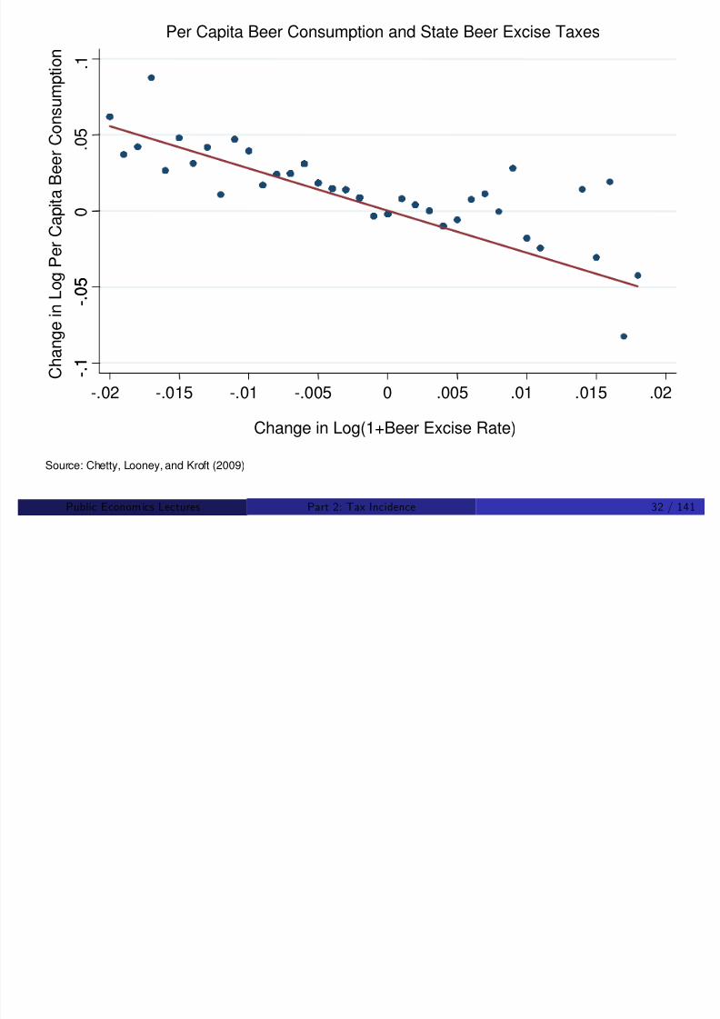
Per Capita Beer Consumption and State Beer Excise Taxes
t i o n
8/8/2019 Chetty - Public Economics Lectures
http://slidepdf.com/reader/full/chetty-public-economics-lectures 60/949
. 0 5
-.02 -.015 -.01 -.005 0 .005 .01 .015 .02 C h a n g e i n L o g P e r C a p i t a B e e r C
o n s u m p
Change in Log(1+Beer Excise Rate)
0
- . 1
- . 0 5
- . 1
- . 0 5
Source: Chetty, Looney, and Kroft (2009)
Public Econom ics Lectures () Part 2: Tax Incidence 32 / 141

8/8/2019 Chetty - Public Economics Lectures
http://slidepdf.com/reader/full/chetty-public-economics-lectures 61/949
8/8/2019 Chetty - Public Economics Lectures
http://slidepdf.com/reader/full/chetty-public-economics-lectures 62/949
Tax Incidence with Salience E¤ects

8/8/2019 Chetty - Public Economics Lectures
http://slidepdf.com/reader/full/chetty-public-economics-lectures 63/949
Let fx (p , t , Z ), y (p , t , Z )g denote empirically observed demands
Place no structure on these demand functions except for feasibility:
(p + t )x (p , t , Z ) + y (p , t , Z ) = Z
Demand functions taken as empirically estimated objects rather than
optimized demand from utility maximization
Supply side model same as above
Market clearing price p satis…es
D (p , t , Z ) = S (p )
where D (p , t , z ) = x (p , t , z ) is market demand for x .
Public Econom ics Lectures () Part 2: Tax Incidence 35 / 141

8/8/2019 Chetty - Public Economics Lectures
http://slidepdf.com/reader/full/chetty-public-economics-lectures 64/949

8/8/2019 Chetty - Public Economics Lectures
http://slidepdf.com/reader/full/chetty-public-economics-lectures 65/949

8/8/2019 Chetty - Public Economics Lectures
http://slidepdf.com/reader/full/chetty-public-economics-lectures 66/949

8/8/2019 Chetty - Public Economics Lectures
http://slidepdf.com/reader/full/chetty-public-economics-lectures 67/949

8/8/2019 Chetty - Public Economics Lectures
http://slidepdf.com/reader/full/chetty-public-economics-lectures 68/949

8/8/2019 Chetty - Public Economics Lectures
http://slidepdf.com/reader/full/chetty-public-economics-lectures 69/949
Evans, Ringel, and Stech (1999)

8/8/2019 Chetty - Public Economics Lectures
http://slidepdf.com/reader/full/chetty-public-economics-lectures 70/949
Exploit state-level changes in excise tax rates to characterizeaggregate market for cigarettes (prices, quantities)
Provides a good introduction to standard di¤-in-di¤ methods
Idea: Suppose federal govt. implements a tax change. Comparecigarette prices before and after the change
D = [P A1 P A0]
Underlying assumption: absent the tax change, there would havebeen no change in cigarette price.
Public Econom ics Lectures () Part 2: Tax Incidence 42 / 141
Di¤erence-in-Di¤erence

8/8/2019 Chetty - Public Economics Lectures
http://slidepdf.com/reader/full/chetty-public-economics-lectures 71/949
But what if price ‡uctuates because of climatic conditions, or if thereis an independent trend in demand?
!First di¤erence (and time series) estimate biased
Can improve on the di¤erence by using di¤-in-di¤
DD = [P A1 P A0] [P B 1 P B 0]
State A: experienced a tax change (treatment)
State B : does not experience any tax change (control)
Identifying assumption: “parallel trends:” absent the policy change,P 1 P 0 would have been the same for A and B
Public Econom ics Lectures () Part 2: Tax Incidence 43 / 141

8/8/2019 Chetty - Public Economics Lectures
http://slidepdf.com/reader/full/chetty-public-economics-lectures 72/949
Parallel Trend Assumption

8/8/2019 Chetty - Public Economics Lectures
http://slidepdf.com/reader/full/chetty-public-economics-lectures 73/949
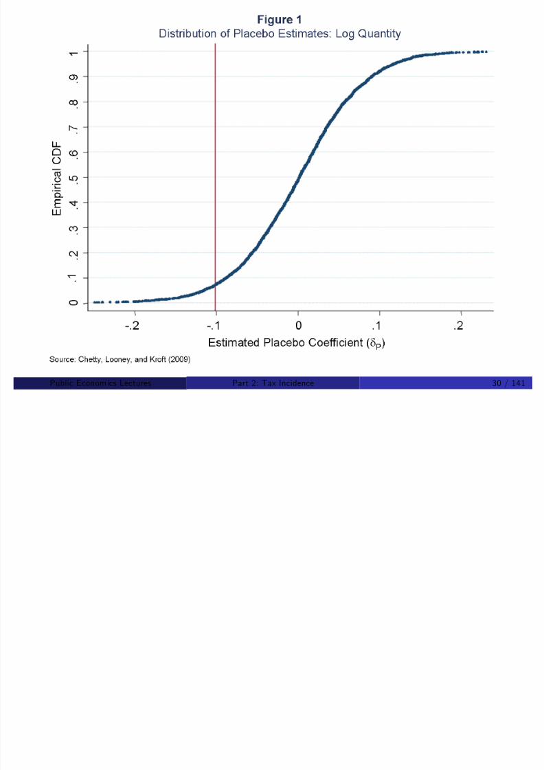
Can use placebo DD to test parallel trend assumption
Compute DD for prior periods!if not zero, then DD t =1 prob. biased
Useful to plot long time series of outcomes for treatment and control
Pattern should be parallel lines, with sudden change just after reform
Want treat. and cntrl. as similar as possible
Can formalize this logic using a permutation test: pretend reformoccurred at other points and replicate estimate
Public Econom ics Lectures () Part 2: Tax Incidence 45 / 141
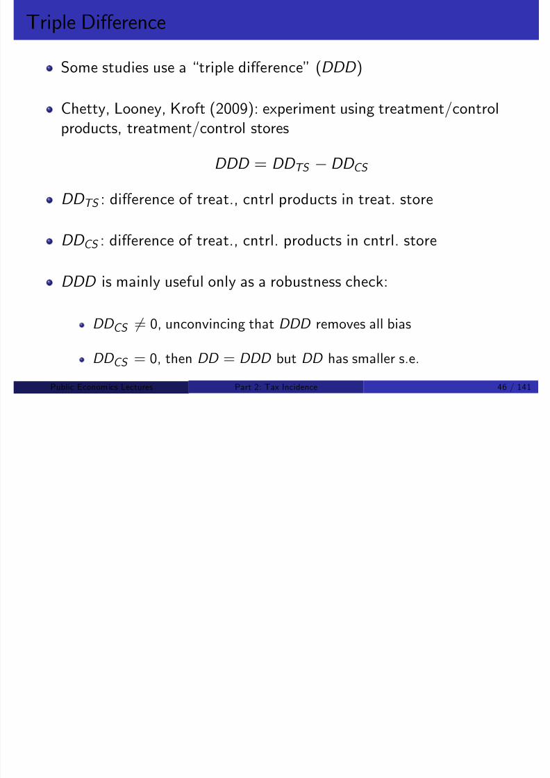
Triple Di¤erence
Some studies use a “triple di¤erence” (DDD)
8/8/2019 Chetty - Public Economics Lectures
http://slidepdf.com/reader/full/chetty-public-economics-lectures 74/949
Some studies use a triple di¤erence (DDD )
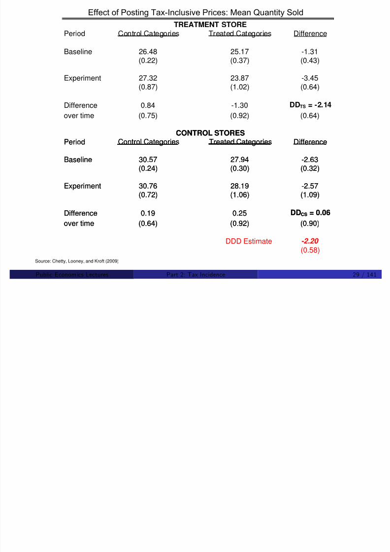
Chetty, Looney, Kroft (2009): experiment using treatment/controlproducts, treatment/control stores
DDD = DD TS DD CS
DD TS : di¤erence of treat., cntrl products in treat. store
DD CS : di¤erence of treat., cntrl. products in cntrl. store
DDD is mainly useful only as a robustness check:
DD CS 6= 0, unconvincing that DDD removes all bias
DD CS = 0, then DD = DDD but DD has smaller s.e.
Public Econom ics Lectures () Part 2: Tax Incidence 46 / 141
Fixed E¤ects
ERS have data for 50 states, 30 years, and many tax changes

8/8/2019 Chetty - Public Economics Lectures
http://slidepdf.com/reader/full/chetty-public-economics-lectures 75/949
y y g
Want to pool all this data to obtain single incidence estimate
Fixed e¤ects: generalize DD with S > 2 periods and J > 2 groups
Suppose that group j in year t experiences policy T of intensity T jt
Want to identify e¤ect of T on price P . OLS regression:
P jt = α + βT jt + jt
With no …xed e¤ects, the estimate of β is biased if treatment T jt
iscorrelated with jt
Often the case in practice - states with taxes di¤er in many ways (e.g.more anti-tobacco campaigns)
Public Econom ics Lectures () Part 2: Tax Incidence 47 / 141
Fixed E¤ects

8/8/2019 Chetty - Public Economics Lectures
http://slidepdf.com/reader/full/chetty-public-economics-lectures 76/949
Include time and state dummies as a way of solving this problem:
P jt = α + γt + δ j + βT jt + jt
Fixed e¤ect regression is equivalent to partial regression
P jt = βT jt + jt
where P jt = P jt P j P t and b T jt is de…ned analogously
Identi…cation obtained from within-state variation over time
Note: common changes that apply to all groups (e.g. fed tax change)captured by time dummy; not a source of variation that identi…es β
Public Econom ics Lectures () Part 2: Tax Incidence 48 / 141
Fixed E¤ects vs. Di¤erence-in-Di¤erence
8/8/2019 Chetty - Public Economics Lectures
http://slidepdf.com/reader/full/chetty-public-economics-lectures 77/949
Advantage relative to DD : more precise, robust results
Disadvantage: …xed e¤ects is a black-box regression, more di¢cult tocheck trends visually as can be done with a single change
! Combine it with simple, graphical, non-parametric evidence
Same parallel trends identi…cation assumption as DD
Potential violation: policy reforms may respond to trends in outcomes
Ex: tobacco prices increase ! state decides to lower tax rate
Public Econom ics Lectures () Part 2: Tax Incidence 49 / 141

8/8/2019 Chetty - Public Economics Lectures
http://slidepdf.com/reader/full/chetty-public-economics-lectures 78/949

8/8/2019 Chetty - Public Economics Lectures
http://slidepdf.com/reader/full/chetty-public-economics-lectures 79/949
Public Econom ics Lectures () Part 2: Tax Incidence 51 / 141
Evans, Ringel, and Stech: Incidence Results

8/8/2019 Chetty - Public Economics Lectures
http://slidepdf.com/reader/full/chetty-public-economics-lectures 80/949
100% pass through implies supply elasticity of εS = ∞ at state level
Could be di¤erent at national level
Important to understand how the variation you are using determineswhat parameter you are identifying
Public Econom ics Lectures () Part 2: Tax Incidence 52 / 141

8/8/2019 Chetty - Public Economics Lectures
http://slidepdf.com/reader/full/chetty-public-economics-lectures 81/949
Evans, Ringel, and Stech: Demand Elasticity

8/8/2019 Chetty - Public Economics Lectures
http://slidepdf.com/reader/full/chetty-public-economics-lectures 82/949
Demand model estimate implies that: εD = 0.42
! 10% increase in price induces a 4.2% reduction in consumption
Tax passed 1-1 onto consumers, so we can compute εD from ˆ β in
demand model:
εD =P
Q
∆Q
∆T = ˆ β/(∆T /P )
taking P and Q average values in the data
Can substitute ∆P = ∆T here because of 1-1 pass through
Public Econom ics Lectures () Part 2: Tax Incidence 54 / 141
IV Estimation of Price Elasticities
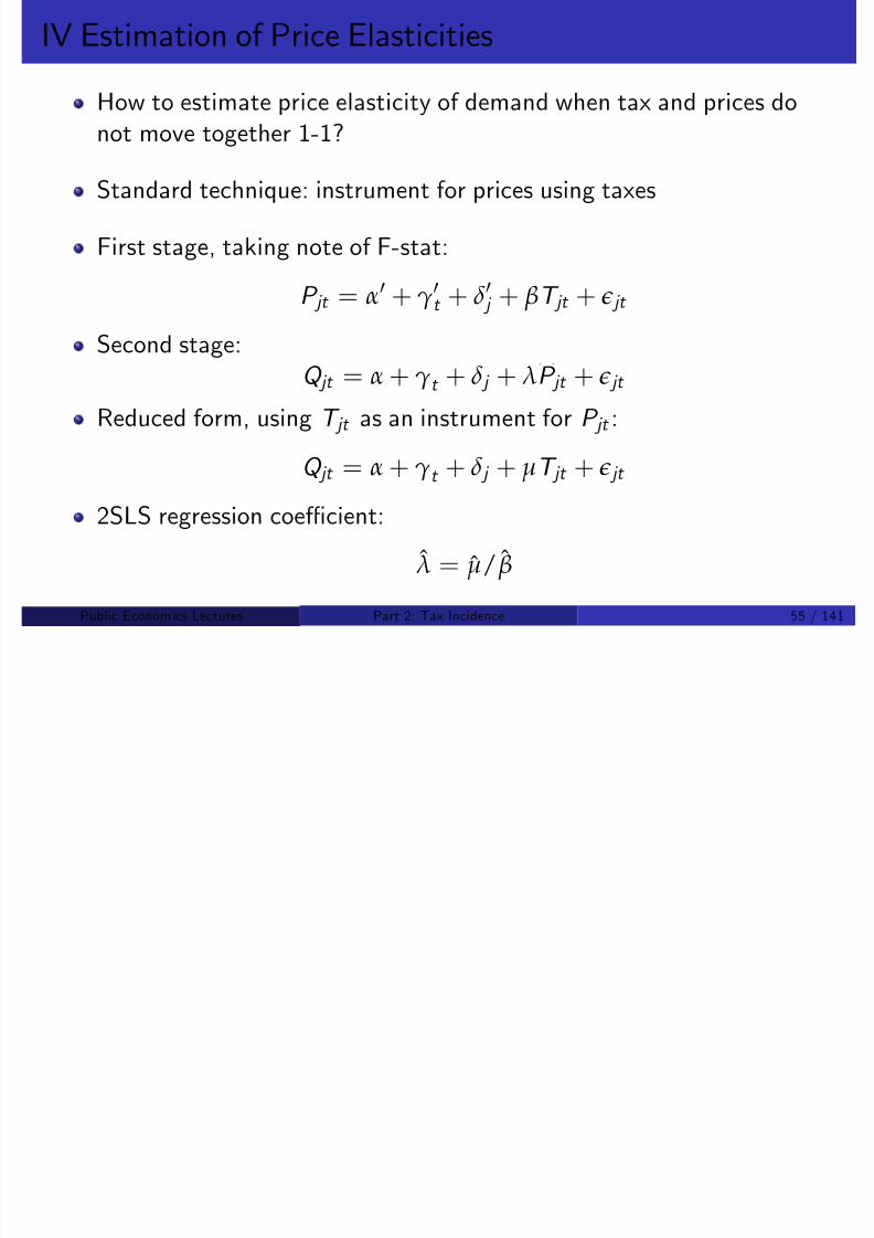
How to estimate price elasticity of demand when tax and prices dot t th 1 1?
8/8/2019 Chetty - Public Economics Lectures
http://slidepdf.com/reader/full/chetty-public-economics-lectures 83/949
not move together 1-1?
Standard technique: instrument for prices using taxes
First stage, taking note of F-stat:
P jt = α0 + γ0t + δ0 j + βT jt + jt
Second stage:Q jt = α + γt + δ j + λ b P jt + jt
Reduced form, using T jt as an instrument for P jt :
Q jt = α + γt + δ j + µT jt + jt
2SLS regression coe¢cient:
λ = µ/ˆ β
Public Econom ics Lectures () Part 2: Tax Incidence 55 / 141
Evans, Ringel, and Stech: Long Run Elasticity

8/8/2019 Chetty - Public Economics Lectures
http://slidepdf.com/reader/full/chetty-public-economics-lectures 84/949
DD before and after one year captures short term response: e¤ect of
current price P jt on current consumption Q jt
F.E. also captures short term responses
What if full response takes more than one period? Especiallyimportant considering nature of cigarette use
F.E. estimate biased. One solution: include lags (T j ,t 1, T j ,t 2, ...).
Are identi…cation assumptions still valid here? Tradeo¤ between LRand validity of identi…cation assumptions
Public Econom ics Lectures () Part 2: Tax Incidence 56 / 141
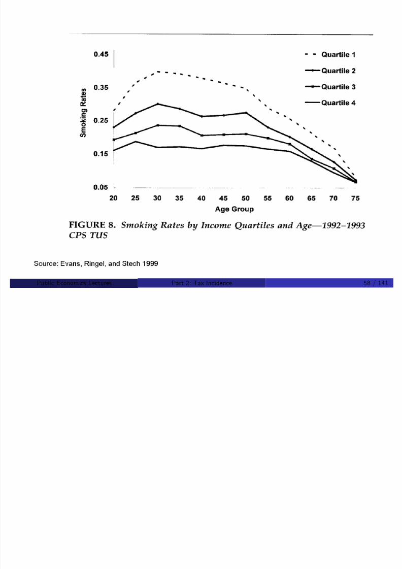
Evans, Ringel, and Stech: Distributional Incidence

8/8/2019 Chetty - Public Economics Lectures
http://slidepdf.com/reader/full/chetty-public-economics-lectures 85/949
Use individual data to see who smokes by education group andincome level
Spending per capita decreases with the income level
Tax is regressive on an absolute level (not only that share of taxesrelative to income goes down)
Conclusion: Taxes/…nes levied on cigarette companies lead to poor
paying more for same goods, with no impact on companies!
Public Econom ics Lectures () Part 2: Tax Incidence 57 / 141
8/8/2019 Chetty - Public Economics Lectures
http://slidepdf.com/reader/full/chetty-public-economics-lectures 86/949
Public Econom ics Lectures () Part 2: Tax Incidence 58 / 141
Cigarette Tax Incidence: Other Considerations
1 Lifetime vs. current incidence (Poterba 1989)

8/8/2019 Chetty - Public Economics Lectures
http://slidepdf.com/reader/full/chetty-public-economics-lectures 87/949
Finds cigarette, gasoline and alcohol taxation are less regressive (instatutory terms) from a lifetime perspectiveHigh corr. between income and cons share in cross-section; weakercorr. with permanent income.
2 Behavioral models (Gruber and Koszegi 2004)
If agents have self control problems, incidence conc. on poor isbene…cial to the extent that they smoke less
3 Intensive vs. extensive margin: Adda and Cornaglia (2006)
Use data on cotinine (biomarker) levels in lungs to measure inhalationHigher taxes lead to fewer cigarettes smoked but no e¤ect on cotininein lungs, implying longer inhalation of each cigarette
Public Econom ics Lectures () Part 2: Tax Incidence 59 / 141
Hastings and Washington 2008

8/8/2019 Chetty - Public Economics Lectures
http://slidepdf.com/reader/full/chetty-public-economics-lectures 88/949
Question: How does food stamps subsidy a¤ect grocery store pricing?
Food stamps typically arrive at the same time for a large group of people, e.g. …rst of the month
Use this variation to study:
1 Whether demand changes at beginning of month (violating PIH)
2 How much of the food stamp bene…t is taken by …rms by increased
prices rather than consumers (intended recipients)
Public Econom ics Lectures () Part 2: Tax Incidence 60 / 141
Hastings and Washington: Data

8/8/2019 Chetty - Public Economics Lectures
http://slidepdf.com/reader/full/chetty-public-economics-lectures 89/949
Scanner data from several grocery stores in Nevada
Data from stores in high-poverty areas (>15% food stamp recipients)and in low-poverty areas (<3%)
Club card data on whether each individual used food stamps
Data from other states where food stamps are staggered acrossmonth used as a control
Research design: use variation across stores, individuals, and time of month to measure pricing responses
Public Econom ics Lectures () Part 2: Tax Incidence 61 / 141

8/8/2019 Chetty - Public Economics Lectures
http://slidepdf.com/reader/full/chetty-public-economics-lectures 90/949

8/8/2019 Chetty - Public Economics Lectures
http://slidepdf.com/reader/full/chetty-public-economics-lectures 91/949
Public Econom ics Lectures () Part 2: Tax Incidence 63 / 141

8/8/2019 Chetty - Public Economics Lectures
http://slidepdf.com/reader/full/chetty-public-economics-lectures 92/949
Public Econom ics Lectures () Part 2: Tax Incidence 64 / 141
Hastings and Washington: Results
Demand increases by 30% in 1st week, prices by about 3%
f f

8/8/2019 Chetty - Public Economics Lectures
http://slidepdf.com/reader/full/chetty-public-economics-lectures 93/949
Very compelling because of multiple dimensions of tests:
cross-individual, cross-store, cross-category, and cross-state
Areas for future work:
1 Pricing outside of supermarkets; many other outlets where food stamps
are used may change prices di¤erently2 Incidence e¤ects for goods other than groceries could be very di¤erent
(car prices and EITC payments)
Interesting theoretical implication: subisidies in markets where
low-income recipients are pooled with others have betterdistributional e¤ects
May favor food stamps as a way to transfer money to low incomesrelative to subsidy such as EITC
Public Econom ics Lectures () Part 2: Tax Incidence 65 / 141
Rothstein 2008
Ho does EITC a¤ect ages?
8/8/2019 Chetty - Public Economics Lectures
http://slidepdf.com/reader/full/chetty-public-economics-lectures 94/949
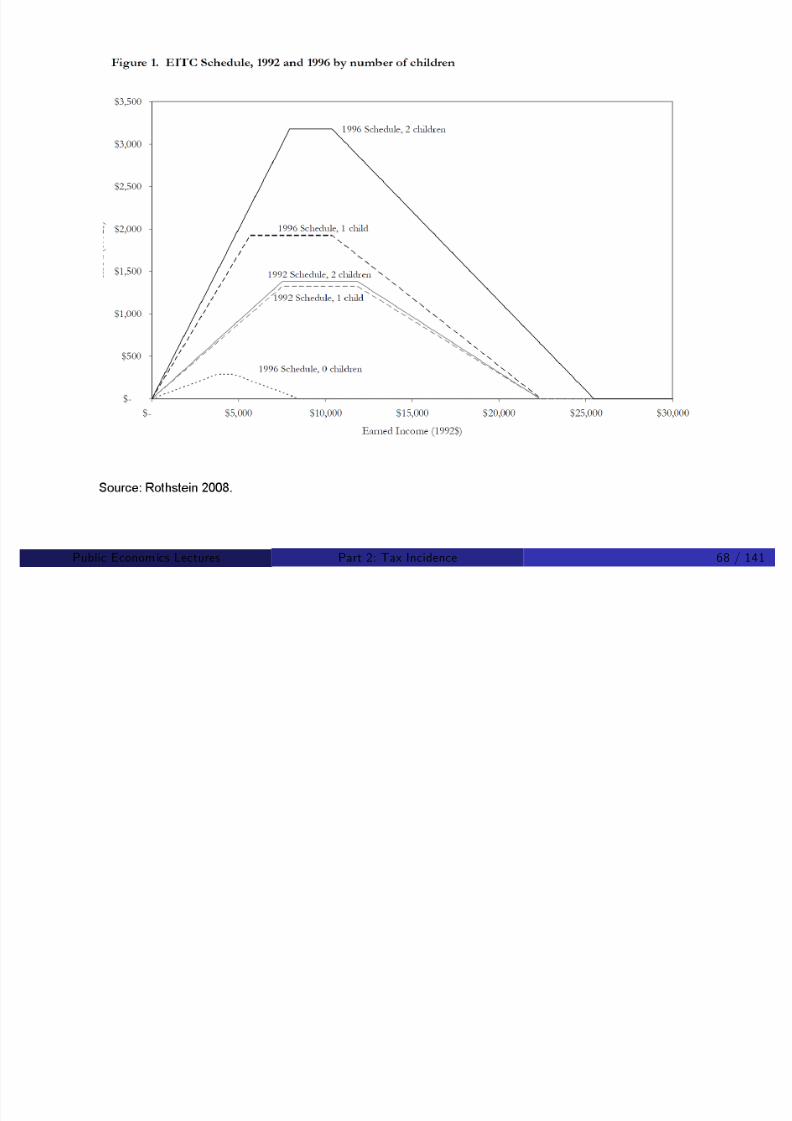
How does EITC a¤ect wages?
EITC payments subsidize work and transfer money to low incomeworking individuals ($50 bil/year)
This subsidy could be taken by employers by shifting wage
Ex: inelastic demand for low-skilled labor and elastic supply ! wagerate adjusts 1-1 with EITC
Policy question: are we actually transferring money to low incomesthrough this program or are we just helping business owners?
Public Econom ics Lectures () Part 2: Tax Incidence 66 / 141
Rothstein 2008
Rothstein considers a simple model of the labor market with threef

8/8/2019 Chetty - Public Economics Lectures
http://slidepdf.com/reader/full/chetty-public-economics-lectures 95/949
types of agents
1 Employers2 EITC-eligible workers3 EITC-ineligible workers
Extends standard partial eq incidence model to allow for di¤erentiatedlabor supply and di¤erent tax rates across demographic groups
Heterogeneity both complicates the analysis and permits identi…cation
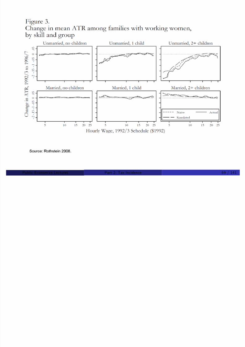
Identi…cation strategy: compare wage changes across groups whowere a¤ected di¤erently by expansions of EITC program from 1992-94
Public Econom ics Lectures () Part 2: Tax Incidence 67 / 141
8/8/2019 Chetty - Public Economics Lectures
http://slidepdf.com/reader/full/chetty-public-economics-lectures 96/949
Public Econom ics Lectures () Part 2: Tax Incidence 68 / 141
8/8/2019 Chetty - Public Economics Lectures
http://slidepdf.com/reader/full/chetty-public-economics-lectures 97/949
P blic Econom ics Lect res () Part 2 Ta Incidence 69 / 141
Rothstein: Empirical Strategy
Two main challenges to identi…cation:

8/8/2019 Chetty - Public Economics Lectures
http://slidepdf.com/reader/full/chetty-public-economics-lectures 98/949
1 EITC 1992-1994 expansion when nation coming out of recession! Compare to other workers (EITC ineligible, slightly higher incomes)
2 Violation of common trends assumption: technical change, moredemand for low-skilled workers in 1990s.! Compare to trends in pre-period (essentially a DDD strategy)
Two dependent variables of interest:
1 [Prices] Measure how wages change for a worker of given skill2 [Quantities] Measure how demand and supply for workers of each skill
type change because of EITC
Basic concept: use two moments – wage and quantity changes toback out slopes of supply and demand curves
P bli E i L t () P t 2 T I id 70 / 141
Rothstein: Empirical Strategy

8/8/2019 Chetty - Public Economics Lectures
http://slidepdf.com/reader/full/chetty-public-economics-lectures 99/949
Ideal test: measure how wage of a given individual changes whenEITC is introduced relative to a similar but ineligible individual
Problem: data is CPS repeated cross-sections. Cannot track “sameindividual.”
Moreover, wage rigidities may prevent cuts for existing employees.
Solution: reweighting procedure to track “same skill” worker over
time (DiNardo, Fortin, and Lemieux 1996)
P bli E i L t () P t 2 T I id 71 / 141
DFL Reweighting
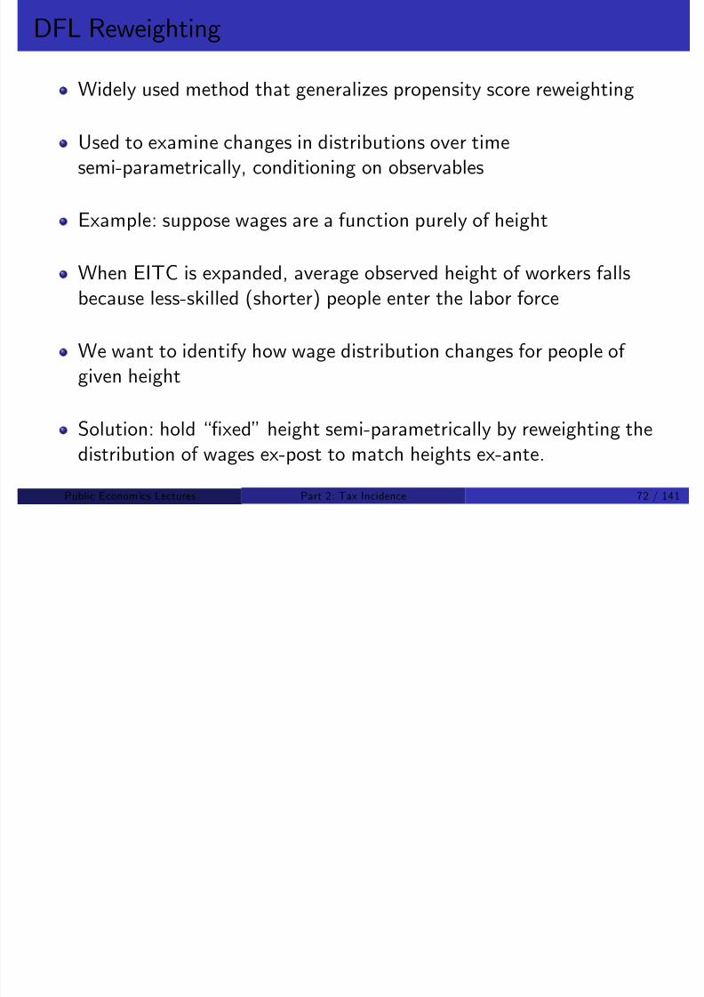
Widely used method that generalizes propensity score reweighting
8/8/2019 Chetty - Public Economics Lectures
http://slidepdf.com/reader/full/chetty-public-economics-lectures 100/949
Used to examine changes in distributions over timesemi-parametrically, conditioning on observables
Example: suppose wages are a function purely of height
When EITC is expanded, average observed height of workers fallsbecause less-skilled (shorter) people enter the labor force
We want to identify how wage distribution changes for people of
given height
Solution: hold “…xed” height semi-parametrically by reweighting thedistribution of wages ex-post to match heights ex-ante.
P bli E i L t () P t 2 T I id 72 / 141
8/8/2019 Chetty - Public Economics Lectures
http://slidepdf.com/reader/full/chetty-public-economics-lectures 101/949

8/8/2019 Chetty - Public Economics Lectures
http://slidepdf.com/reader/full/chetty-public-economics-lectures 102/949
Public Econom ics Lectures () Part 2: Tax Incidence 74 / 141

8/8/2019 Chetty - Public Economics Lectures
http://slidepdf.com/reader/full/chetty-public-economics-lectures 103/949
Public Econom ics Lectures () Part 2: Tax Incidence 75 / 141

8/8/2019 Chetty - Public Economics Lectures
http://slidepdf.com/reader/full/chetty-public-economics-lectures 104/949

8/8/2019 Chetty - Public Economics Lectures
http://slidepdf.com/reader/full/chetty-public-economics-lectures 105/949
Rothstein: Results

8/8/2019 Chetty - Public Economics Lectures
http://slidepdf.com/reader/full/chetty-public-economics-lectures 106/949
Basic DFL comparisons yield perverse result: groups that bene…tedfrom EITC and started working more had more wage growth
Potential explanation: demand curve shifted di¤erentially – higherdemand for low skilled workers in 1990s.
To deal with this, repeats same analysis for 1989-1992 (no EITCexpansion) and takes di¤erences
Changes sign back to expected, but imprecisely estimated
Public Econom ics Lectures () Part 2: Tax Incidence 78 / 141

8/8/2019 Chetty - Public Economics Lectures
http://slidepdf.com/reader/full/chetty-public-economics-lectures 107/949
Rothstein: Results
Ultimately uses quantity estimates and incidence formula to back outpredicted changes

8/8/2019 Chetty - Public Economics Lectures
http://slidepdf.com/reader/full/chetty-public-economics-lectures 108/949
Wage elasticity estimates: 0.7 for labor supply, 0.3 for labor demand
Implications using formulas from model:
EITC-eligible workers gain $0.70 per $1 EITC expansion
Employers gain about $0.70
EITC-ineligible low-skilled workers lose about $0.40
On net, achieve only $0.30 of redistribution toward low incomeindividuals for every $1 of EITC
Public Econom ics Lectures () Part 2: Tax Incidence 80 / 141
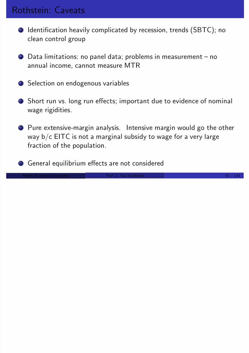
Rothstein: Caveats
1 Identi…cation heavily complicated by recession, trends (SBTC); noclean control group
8/8/2019 Chetty - Public Economics Lectures
http://slidepdf.com/reader/full/chetty-public-economics-lectures 109/949
2 Data limitations: no panel data; problems in measurement – noannual income, cannot measure MTR
3 Selection on endogenous variables
4 Short run vs. long run e¤ects; important due to evidence of nominalwage rigidities.
5 Pure extensive-margin analysis. Intensive margin would go the other
way b/c EITC is not a marginal subsidy to wage for a very largefraction of the population.
6 General equilibrium e¤ects are not considered
Public Econom ics Lectures () Part 2: Tax Incidence 81 / 141
Extensions of Basic Partial Equilibrium Analysis
1 Market rigidities:

8/8/2019 Chetty - Public Economics Lectures
http://slidepdf.com/reader/full/chetty-public-economics-lectures 110/949
With price ‡oors, incidence can di¤er
Consider incidence of social security taxes with minimum wage
Statutory incidence: 6.2% on employer and 6.2% on employee
Share of each should not matter as long as total is constant becausewages will fall to adjust
But with binding minimum wage, employers cannot cut wage further,so statutory incidence determines economic incidence on the margin
Public Econom ics Lectures () Part 2: Tax Incidence 82 / 141

8/8/2019 Chetty - Public Economics Lectures
http://slidepdf.com/reader/full/chetty-public-economics-lectures 111/949
Extensions of Basic Partial Equilibrium Analysis
1 Market rigidities

8/8/2019 Chetty - Public Economics Lectures
http://slidepdf.com/reader/full/chetty-public-economics-lectures 112/949
2 Imperfect competition
3 E¤ects on other markets:
Increase in cigarette tax ! substitute cigarettes for cigars, increasingprice of cigars and shifting cigarette demand curve
Revenue e¤ects on other markets: tax increases make agents poorer;less to spend on other markets
This motivates general equilibrium analysis of incidence
Public Econom ics Lectures () Part 2: Tax Incidence 84 / 141
General Equilibrium Analysis
Trace out full incidence of taxes back to original owners of factors

8/8/2019 Chetty - Public Economics Lectures
http://slidepdf.com/reader/full/chetty-public-economics-lectures 113/949
Partial equilibrium: “producer” vs. consumer
General equilibrium: capital owners vs. labor vs. landlords, etc.
Two types of models:
1 Static: many sectors or many factors of production
Workhorse analytical model: Harberger (1962): 2 sector and 2 factorsof productionComputational General Equilibrium: many sectors, many factors of production model
2 Dynamic
Intergenerational incidence: Soc Sec reformAsset price e¤ects: capitalization
Public Econom ics Lectures () Part 2: Tax Incidence 85 / 141

8/8/2019 Chetty - Public Economics Lectures
http://slidepdf.com/reader/full/chetty-public-economics-lectures 114/949
Harberger Model: SetupProduction in sectors 1 (bikes) and 2 (cars):
X 1 = F 1(K 1, L1) = L1f (k 1)

8/8/2019 Chetty - Public Economics Lectures
http://slidepdf.com/reader/full/chetty-public-economics-lectures 115/949
X 2 = F 2(K 2, L2) = L2f (k 2)with full employment conditions K 1 + K 2 = K and L1 + L2 = L
Factors w and L fully mobile ! in eq., returns must be equal:
w = p 1F 1L = p 2F 2Lr = p 1F 1K = p 2F 2K
Demand functions for goods 1 and 2:
X 1 = X 1(p 1/p 2) and X 2 = X 2(p 1/p 2)
Note: all consumers identical so redistribution of incomes via taxsystem does not a¤ect demand via a feedback e¤ect
System of ten eq’ns and ten unknowns: K i , Li , p i , X i , w , r
Public Econom ics Lectures () Part 2: Tax Incidence 87 / 141
Harberger Model: E¤ect of Tax Increase
Introduce small tax d τ on rental of capital in sector 2 (K 2)
All eqns the same as above except r = (1 d τ )p 2F 2K

8/8/2019 Chetty - Public Economics Lectures
http://slidepdf.com/reader/full/chetty-public-economics-lectures 116/949
Linearize the 10 eq’ns around initial equilibrium to compute the e¤ectof d τ on all 10 variables (dw , dr , dL1, ...)
Labor income = wL with L …xed, rK = capital income with K …xed
Therefore change in prices dw /d τ and dr /d τ describes how tax isshifted from capital to labor
Changes in prices dp 1/d τ , dp 2/d τ describe how tax is shifted from
sector 2 to sector 1
Kotliko¤ and Summers (Section 2.2) state linearized equations as afn. of substitution elasticities
Public Econom ics Lectures () Part 2: Tax Incidence 88 / 141

8/8/2019 Chetty - Public Economics Lectures
http://slidepdf.com/reader/full/chetty-public-economics-lectures 117/949

8/8/2019 Chetty - Public Economics Lectures
http://slidepdf.com/reader/full/chetty-public-economics-lectures 118/949
Harberger Model: Main E¤ects
3. Substitution + Output = Overshifting e¤ects

8/8/2019 Chetty - Public Economics Lectures
http://slidepdf.com/reader/full/chetty-public-economics-lectures 119/949
Case 1: K 1/L1 < K 2/L2
Can get overshifting of tax, dr < d τ and dw > 0
Capital bears more than 100% of the burden if output e¤ect su¢cientlystrong
Taxing capital in sector 2 raises prices of cars ! more demand forbikes, less demand for cars
With very elastic demand (two goods are highly substitutable), demand
for labor rises sharply and demand for capital falls sharply
Capital loses more than direct tax e¤ect and labor suppliers gain
Public Econom ics Lectures () Part 2: Tax Incidence 91 / 141
Harberger Model: Main E¤ects3. Substitution + Output = Overshifting e¤ects
Case 2 : K 1/L1 > K 2/L2

8/8/2019 Chetty - Public Economics Lectures
http://slidepdf.com/reader/full/chetty-public-economics-lectures 120/949
Possible that capital is made better o¤ by capital tax
Labor forced to bear more than 100% of incidence of capital tax insector 2
Ex. Consider tax on capital in bike sector: demand for bikes falls,demand for cars rises
Capital in greater demand than it was before ! price of labor falls
substantially, capital owners actually gain
Bottom line: taxed factor may bear less than 0 or more than 100% of tax.
Public Econom ics Lectures () Part 2: Tax Incidence 92 / 141
Harberger Two Sector ModelTheory not very informative: model mainly used to illustrate negativeresult that “anything goes”

8/8/2019 Chetty - Public Economics Lectures
http://slidepdf.com/reader/full/chetty-public-economics-lectures 121/949
More interest now in developing methods to identify what actuallyhappens
Original Application of this framework by Harberger: sectors =housing and corporations
Capital in these sectors taxed di¤erently because of corporate incometax and many tax subsidies to housing
Ex: Deductions for mortgage interest and prop. tax are about $50 bn
total
Harberger made assumptions about elasticities and calculatedincidence of corporate tax given potential to substitute into housing
Public Econom ics Lectures () Part 2: Tax Incidence 93 / 141
Computable General Equilibrium Models
Harberger analyzed two sectors; subsequent literature expandedanalysis to multiple sectors

8/8/2019 Chetty - Public Economics Lectures
http://slidepdf.com/reader/full/chetty-public-economics-lectures 122/949
Analytical methods infeasible in multi-sector models
Instead, use numerical simulations to investigate tax incidence e¤ects
after specifying full model
Pioneered by Shoven and Whalley (1972). See Kotliko¤ andSummers section 2.3 for a review
Produced a voluminous body of research in PF, trade, anddevelopment economics
Public Econom ics Lectures () Part 2: Tax Incidence 94 / 141
CGE Models: General Structure
N intermediate production sectors

8/8/2019 Chetty - Public Economics Lectures
http://slidepdf.com/reader/full/chetty-public-economics-lectures 123/949
M …nal consumption goods
J groups of consumers who consume products and supply labor
Each industry has di¤erent substitution elasticities for capital andlabor
Each consumer group has Cobb-Douglas utility over M consumptiongoods with di¤erent parameters
Specify all these parameters (calibrated to match some elasticities)and then simulate e¤ects of tax changes
Public Econom ics Lectures () Part 2: Tax Incidence 95 / 141
Criticism of CGE Models
Findings very sensitive to structure of the model: savings behavior,
f

8/8/2019 Chetty - Public Economics Lectures
http://slidepdf.com/reader/full/chetty-public-economics-lectures 124/949
perfect competition assumption
Findings sensitive to size of key behavioral elasticities and functionalform assumptions
Modern econometric methods conceptually not suitable for GEproblems, where the whole point is “spillover e¤ects” (contamination)
Need a new empirical paradigm to deal with these problems – a major
open challenge
Public Econom ics Lectures () Part 2: Tax Incidence 96 / 141
Open Economy Application

8/8/2019 Chetty - Public Economics Lectures
http://slidepdf.com/reader/full/chetty-public-economics-lectures 125/949
Key assumption in Harberger model: both labor and capital perfectlymobile across sectors
Now apply framework to analyze capital taxation in open economies,
where capital is more likely to be mobile than labor
See Kotliko¤ and Summers section 3.1 for a good exposition
Public Econom ics Lectures () Part 2: Tax Incidence 97 / 141
Open Economy Application: Framework

8/8/2019 Chetty - Public Economics Lectures
http://slidepdf.com/reader/full/chetty-public-economics-lectures 126/949
One good, two-factor, two-sector model
Sector 1 : small open economy where L1 is …xed and K 1 mobile
Sector 2 : rest of the world L2 …xed and K 2 mobile
Total capital stock K = K 1 + K 2 is …xed
Public Econom ics Lectures () Part 2: Tax Incidence 98 / 141
Open Economy Application: Framework
Small country introduces tax on capital income (K 1)
Aft t t t b l

8/8/2019 Chetty - Public Economics Lectures
http://slidepdf.com/reader/full/chetty-public-economics-lectures 127/949
After-tax returns must be equal:
r = F 2K = (1 τ )F 1K
Capital ‡ows from 1 to 2 until returns are equalized; if 2 is large
relative to 1, no e¤ect on r
Wage rate w 1 = F 1L(K 1, L1) dec. when K 1 dec. b/c L1 is …xed
Return of capitalists in small country is unchanged; workers in home
country bear the burden of the tax
Taxing capital is bad for workers!
Public Econom ics Lectures () Part 2: Tax Incidence 99 / 141
Open Economy Application: Empirics
M bilit f K d i th i lt

8/8/2019 Chetty - Public Economics Lectures
http://slidepdf.com/reader/full/chetty-public-economics-lectures 128/949
Mobility of K drives the previous result
Empirical question: is K actually mobile across countries?
Two strategies:
1 Test based on prices and equilibrium relationships [Macro …nance]
2 Look at mobility directly [Feldstein and Horioka 1980]
Public Econom ics Lectures () Part 2: Tax Incidence 100 / 141

8/8/2019 Chetty - Public Economics Lectures
http://slidepdf.com/reader/full/chetty-public-economics-lectures 129/949
Feldstein and Horioka 1980
Second strategy: look at capital mobility directly

8/8/2019 Chetty - Public Economics Lectures
http://slidepdf.com/reader/full/chetty-public-economics-lectures 130/949
Feldstein and Horioka use data on OECD countries from 1960-74
Closed economy: S = I ; open economy: S I = X M
Motivates regression:
I /GDP = α + βS /GDP + ...
Find β = 0.89 (0.07)
Public Econom ics Lectures () Part 2: Tax Incidence 102 / 141
Feldstein and Horioka 1980
In closed economy, β = 1

8/8/2019 Chetty - Public Economics Lectures
http://slidepdf.com/reader/full/chetty-public-economics-lectures 131/949
But do not know what β should be in an open economy
β may be close to 1 in open economy if
1 Policy objectives involving S I (trade de…cit balance)
2 Summing over all countries: S = I as imports and exports cancel out
3
Data problem: S constructed from I in some countries
Public Econom ics Lectures () Part 2: Tax Incidence 103 / 141
Open Economy Applications: Empirics
Large subsequent literature runs similar regressions and …nds mixed
results

8/8/2019 Chetty - Public Economics Lectures
http://slidepdf.com/reader/full/chetty-public-economics-lectures 132/949
results
Generally …nds more ‡ow of capital and increasing over time
General view: cannot extract money from capital in small openeconomies
Ex. Europe: tax competition has led to lower capital tax rates
Could explain why state capital taxes are relatively low in the U.S.
Public Econom ics Lectures () Part 2: Tax Incidence 104 / 141
General Equilibrium Incidence in Dynamic Models
Static analysis above assumes that all prices and quantities adjustimmediately

8/8/2019 Chetty - Public Economics Lectures
http://slidepdf.com/reader/full/chetty-public-economics-lectures 133/949
In practice, adjustment of capital stock and reallocation of labor takestime
Dynamic CGE models incorporate these e¤ects; even more complex
Static model can be viewed as description of steady states
During transition path, measured ‡ow prices (r , w ) will not correspondto steady state responses
How to measure incidence in dynamic models?
Public Econom ics Lectures () Part 2: Tax Incidence 105 / 141
Capitalization and the Asset Price Approach
Asset prices can be used to infer incidence in dynamic models(Summers 1983)

8/8/2019 Chetty - Public Economics Lectures
http://slidepdf.com/reader/full/chetty-public-economics-lectures 134/949
Study e¤ect of tax changes on asset prices
Asset prices adjust immediately in e¢cient markets, incorporating thefull present-value of subsequent changes
E¢cient asset markets incorporate all e¤ects on factor costs, outputprices, etc.
Limitation: can only be used to characterize incidence of policies on
capital owners
There are no markets for individuals
Public Econom ics Lectures () Part 2: Tax Incidence 106 / 141
Simple Model of Capitalization E¤ectsFirms pay out pro…ts as dividends
Pro…ts determined by revenues net of factor payments:
V = ∑ Dt = ∑ qt Xt w jt L jt

8/8/2019 Chetty - Public Economics Lectures
http://slidepdf.com/reader/full/chetty-public-economics-lectures 135/949
V = ∑ D 1 + r
= ∑ q X w j Lj
1 + r
Change in valuation of …rm ( dV dt
) re‡ects change in present value of pro…ts
dV dt
is a su¢cient statistic that incorporates changes in all prices
Empirical applications typically use “event study” methodology
Examine pattern of asset prices or returns over time, look for break at
time of announcement of policy change
Problem: clean shocks are rare; big reforms do not happen suddenlyand are always expected to some extent
Public Econom ics Lectures () Part 2: Tax Incidence 107 / 141
Empirical Applications

8/8/2019 Chetty - Public Economics Lectures
http://slidepdf.com/reader/full/chetty-public-economics-lectures 136/949
1 [Cutler 1988] E¤ect of Tax Reform Act of 1986 on corporations
2 [Linden and Rocko¤ 2008] E¤ect of a sex o¤ender moving intoneighborhood on home values
3 [Friedman 2008] E¤ect of Medicare Part D on drug companies
Public Econom ics Lectures () Part 2: Tax Incidence 108 / 141

8/8/2019 Chetty - Public Economics Lectures
http://slidepdf.com/reader/full/chetty-public-economics-lectures 137/949
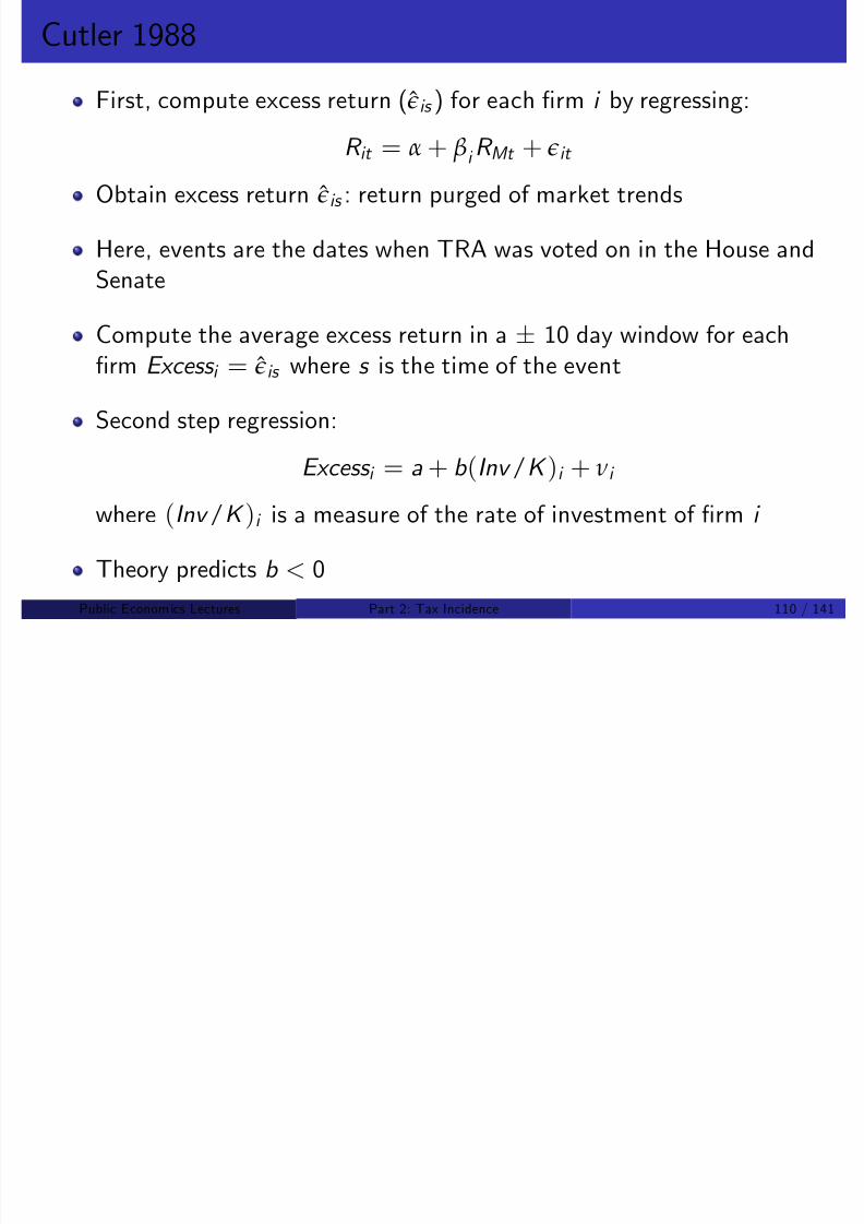
Cutler 1988First, compute excess return (is ) for each …rm i by regressing:
R it = α + βi R Mt + it
Obtain excess return is : return purged of market trends
8/8/2019 Chetty - Public Economics Lectures
http://slidepdf.com/reader/full/chetty-public-economics-lectures 138/949
Obtain excess return : return purged of market trends
Here, events are the dates when TRA was voted on in the House andSenate
Compute the average excess return in a 10 day window for each…rm Excess i = is where s is the time of the event
Second step regression:
Excess i = a + b (Inv /K )i + νi
where (Inv /K )i is a measure of the rate of investment of …rm i
Theory predicts b < 0
Public Econom ics Lectures () Part 2: Tax Incidence 110 / 141
8/8/2019 Chetty - Public Economics Lectures
http://slidepdf.com/reader/full/chetty-public-economics-lectures 139/949
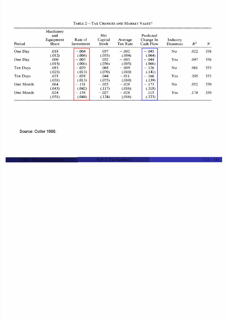
Cutler: Results
Cutler …nds b = 0.029(0.013)
This is consistent with expectations, but other …ndings are not:

8/8/2019 Chetty - Public Economics Lectures
http://slidepdf.com/reader/full/chetty-public-economics-lectures 140/949
p , g
Changes in future tax liabilities not correlated with stock value changes
Responses to two distinct events (passage of bill in House and Senate)
not correlated
Were the votes really surprises? Need data on expectations
Study is somewhat inconclusive because of noisy data
But led to a subsequent better-identi…ed literature
Public Econom ics Lectures () Part 2: Tax Incidence 112 / 141

8/8/2019 Chetty - Public Economics Lectures
http://slidepdf.com/reader/full/chetty-public-economics-lectures 141/949

8/8/2019 Chetty - Public Economics Lectures
http://slidepdf.com/reader/full/chetty-public-economics-lectures 142/949

8/8/2019 Chetty - Public Economics Lectures
http://slidepdf.com/reader/full/chetty-public-economics-lectures 143/949
Public Econom ics Lectures () Part 2: Tax Incidence 115 / 141

8/8/2019 Chetty - Public Economics Lectures
http://slidepdf.com/reader/full/chetty-public-economics-lectures 144/949
Public Econom ics Lectures () Part 2: Tax Incidence 116 / 141

8/8/2019 Chetty - Public Economics Lectures
http://slidepdf.com/reader/full/chetty-public-economics-lectures 145/949

8/8/2019 Chetty - Public Economics Lectures
http://slidepdf.com/reader/full/chetty-public-economics-lectures 146/949
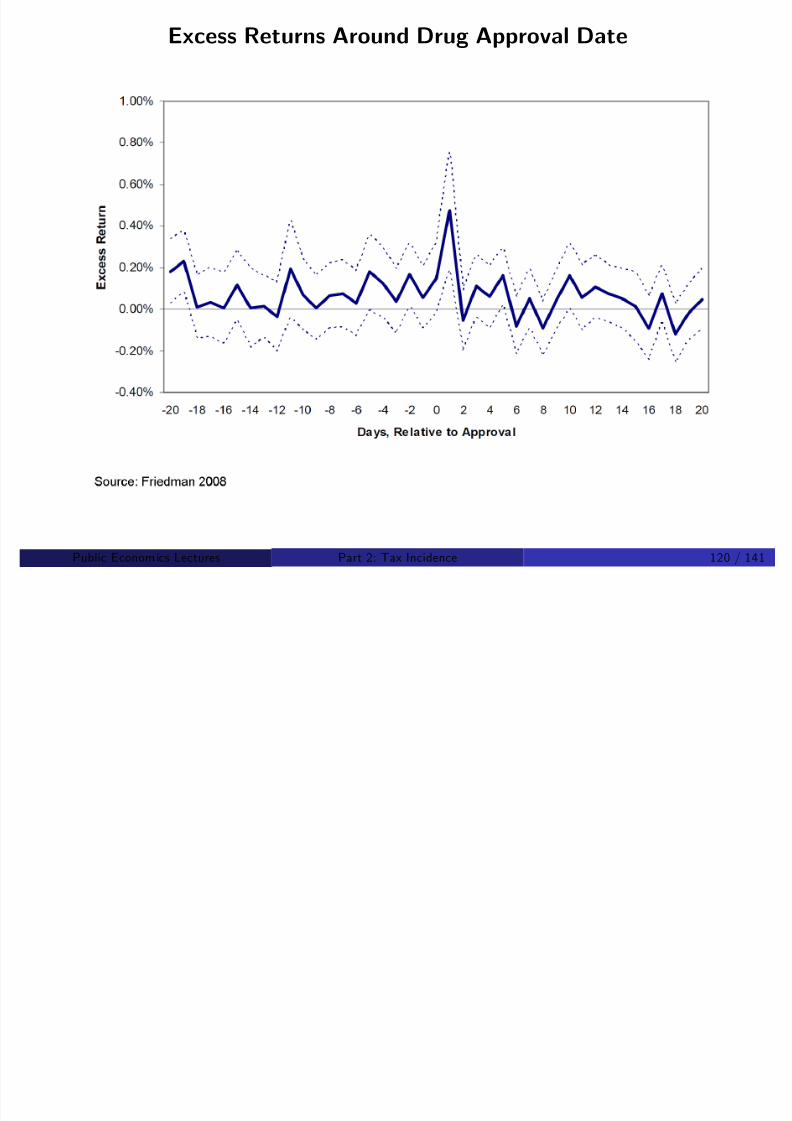
Friedman 2008Medicare part D passed by Congress in 2003; enacted in 2006
Expanded Medicare coverage to include prescription drugs (providedcoverage for 10 mil additional people)
What is the incidence of Medicare part D? How much of the

8/8/2019 Chetty - Public Economics Lectures
http://slidepdf.com/reader/full/chetty-public-economics-lectures 147/949
What is the incidence of Medicare part D? How much of theexpenditure is captured by drug companies through higher pro…ts?
Event study: excess returns for drug companies around FDA approval
of drugs
Tests whether excess returns for high-Medicare share drugs is higherafter Medicare Part D is passed
Let MMS i denote medicare market share drug class i . Second-stage
estimating equation:
Excess i = α + βMMS i + γPost 2003t + λPost 2003t MMS i
Public Econom ics Lectures () Part 2: Tax Incidence 119 / 141
Excess Returns Around Drug Approval Date
8/8/2019 Chetty - Public Economics Lectures
http://slidepdf.com/reader/full/chetty-public-economics-lectures 148/949
Public Econom ics Lectures () Part 2: Tax Incidence 120 / 141

8/8/2019 Chetty - Public Economics Lectures
http://slidepdf.com/reader/full/chetty-public-economics-lectures 149/949

8/8/2019 Chetty - Public Economics Lectures
http://slidepdf.com/reader/full/chetty-public-economics-lectures 150/949

8/8/2019 Chetty - Public Economics Lectures
http://slidepdf.com/reader/full/chetty-public-economics-lectures 151/949

8/8/2019 Chetty - Public Economics Lectures
http://slidepdf.com/reader/full/chetty-public-economics-lectures 152/949
Mandated Bene…ts
Tempting to view mandates as additional taxes on …rms and apply
same analysis as above

8/8/2019 Chetty - Public Economics Lectures
http://slidepdf.com/reader/full/chetty-public-economics-lectures 153/949
But mandated bene…ts have di¤erent e¤ects on equilibrium wagesand employment di¤erently than a tax (Summers 1989)
Key di¤erence: mandates are a bene…t for the worker, so e¤ect onmarket equilibrium depends on bene…ts workers get from the program
Unlike a tax, may have no distortionary e¤ect on employment and
only an incidence e¤ect (lower wages)
Public Econom ics Lectures () Part 2: Tax Incidence 125 / 141
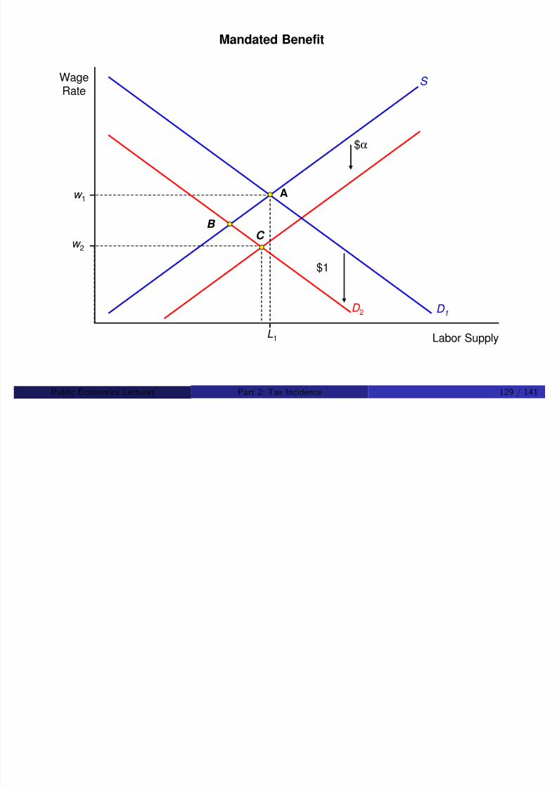
Mandated Bene…ts: Simple Model
Labor demand (D ) and labor supply (S ) are functions of the wage, w
Initial equilibrium:D (w 0) = S (w 0)

8/8/2019 Chetty - Public Economics Lectures
http://slidepdf.com/reader/full/chetty-public-economics-lectures 154/949
Now, govt mandates employers provide a bene…t with cost t
Workers value the bene…t at αt dollars
Typically 0 < α < 1 but α > 1 possible with market failures
Labor cost is now w + t , e¤ective wage w + αt
New equilibrium:D (w + t ) = S (w + αt )
Public Econom ics Lectures () Part 2: Tax Incidence 126 / 141
Mandated Benefit
S WageRate

8/8/2019 Chetty - Public Economics Lectures
http://slidepdf.com/reader/full/chetty-public-economics-lectures 155/949
w 1
L1
D 1
A
Labor Supply
Public Econom ics Lectures () Part 2: Tax Incidence 127 / 141

8/8/2019 Chetty - Public Economics Lectures
http://slidepdf.com/reader/full/chetty-public-economics-lectures 156/949
S WageRate
$α
Mandated Benefit
8/8/2019 Chetty - Public Economics Lectures
http://slidepdf.com/reader/full/chetty-public-economics-lectures 157/949
w 2
w 1
L1
D 1
D 2
$1
A
Labor Supply
C B
Public Econom ics Lectures () Part 2: Tax Incidence 129 / 141
Mandated Bene…ts: Incidence Formula
Analysis for a small t : linear expansion around initial equilibrium
(dw /dt + 1)D 0 = (dw /dt + α)S 0
dw /dt = (D 0 αS 0)/(S 0 D 0)
1 + (1 α)ηS

8/8/2019 Chetty - Public Economics Lectures
http://slidepdf.com/reader/full/chetty-public-economics-lectures 158/949
= 1 + (1 α)ηS
ηS ηD
where
ηD = wD 0/D < 0
ηS = wS 0/S > 0
If α = 1, dw /dt = 1 and no e¤ect on employment
More generally: 0 < α < 1 equivalent to a tax 1 α with usualincidence and e¢ciency e¤ects
Public Econom ics Lectures () Part 2: Tax Incidence 130 / 141
Empirical Applications

8/8/2019 Chetty - Public Economics Lectures
http://slidepdf.com/reader/full/chetty-public-economics-lectures 159/949
1 [Gruber 1994] Pregnancy health insurance costs
2 [Acemoglu and Angrist 2001] Americans with Disabilities Act
Public Econom ics Lectures () Part 2: Tax Incidence 131 / 141

8/8/2019 Chetty - Public Economics Lectures
http://slidepdf.com/reader/full/chetty-public-economics-lectures 160/949
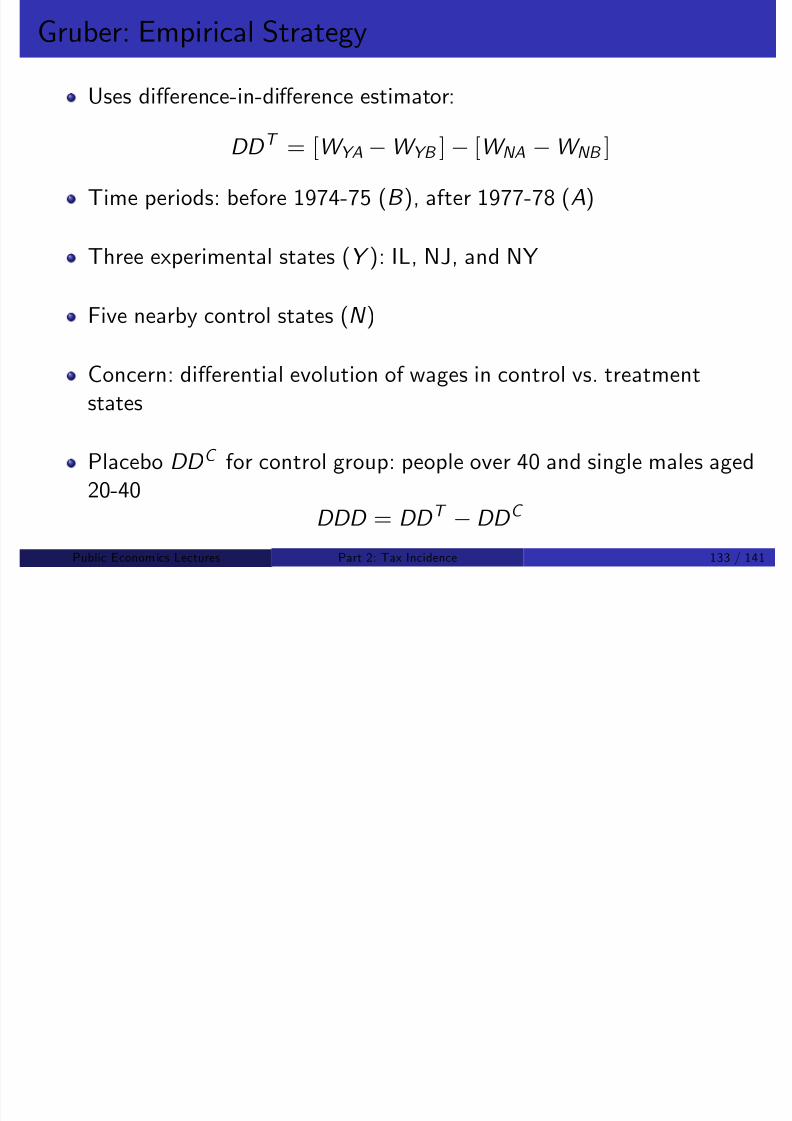
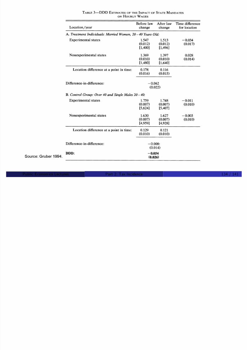
Gruber: Empirical Strategy
Uses di¤erence-in-di¤erence estimator:
DD T = [W YA W YB ] [W NA W NB ]
Time periods: before 1974-75 (B ), after 1977-78 (A)
8/8/2019 Chetty - Public Economics Lectures
http://slidepdf.com/reader/full/chetty-public-economics-lectures 161/949
Three experimental states (Y ): IL, NJ, and NY
Five nearby control states (N )
Concern: di¤erential evolution of wages in control vs. treatmentstates
Placebo DD C for control group: people over 40 and single males aged20-40
DDD = DD T DD C
Public Econom ics Lectures () Part 2: Tax Incidence 133 / 141
8/8/2019 Chetty - Public Economics Lectures
http://slidepdf.com/reader/full/chetty-public-economics-lectures 162/949
Gruber: Results
Find DD T = 0.062(0.022), DDD = 0.054(0.026)
Implies that hourly wage decreases by roughly the cost of themandate (no distortion case, α = 1).

8/8/2019 Chetty - Public Economics Lectures
http://slidepdf.com/reader/full/chetty-public-economics-lectures 163/949
( )
Indirect aggregate evidence also suggests that costs have been shiftedon wages
Share of health care costs in total employee compensation hasincreased substantially over last 30 years
But share of total employee compensation as a share of nationalincome roughly unchanged
Public Econom ics Lectures () Part 2: Tax Incidence 135 / 141
Acemoglu and Angrist 2001
Look at e¤ect of ADA regulations on wages and employment of thedisabled
The 1993 Americans with Disabilities Act requires employers to:

8/8/2019 Chetty - Public Economics Lectures
http://slidepdf.com/reader/full/chetty-public-economics-lectures 164/949
Make accommodations for disabled employees
Pay same wages to disabled employees as to non-disabled workers
Cost to accommodate disabled workers: $1000 per person on average
Theory is ambiguous on net employment e¤ect because of wagediscrimination clause
Public Econom ics Lectures () Part 2: Tax Incidence 136 / 141
S WageRate
Mandated Benefit with Minimum Wage

8/8/2019 Chetty - Public Economics Lectures
http://slidepdf.com/reader/full/chetty-public-economics-lectures 165/949
w 2
w 1
L1
D 1
D 2
A
B
Labor Supply
minimum wage
Public Econom ics Lectures () Part 2: Tax Incidence 137 / 141
Acemoglu and Angrist 2001
Acemoglu and Angrist estimate the impact of act using data from the

8/8/2019 Chetty - Public Economics Lectures
http://slidepdf.com/reader/full/chetty-public-economics-lectures 166/949
Current Population Survey
Examine employment and wages of disabled workers before and afterthe ADA went into e¤ect
Public Econom ics Lectures () Part 2: Tax Incidence 138 / 141

8/8/2019 Chetty - Public Economics Lectures
http://slidepdf.com/reader/full/chetty-public-economics-lectures 167/949
Public Econom ics Lectures () Part 2: Tax Incidence 139 / 141

8/8/2019 Chetty - Public Economics Lectures
http://slidepdf.com/reader/full/chetty-public-economics-lectures 168/949
Public Econom ics Lectures () Part 2: Tax Incidence 140 / 141
Acemoglu and Angrist: Results
Employment of disabled workers fell after the reform:
About a 1.5-2 week drop in employment for males, roughly a 5-10%decline in employment
Wages did not change

8/8/2019 Chetty - Public Economics Lectures
http://slidepdf.com/reader/full/chetty-public-economics-lectures 169/949
g g
Results consistent w/ labor demand elasticity of about -1 or -2
Firms with fewer than 25 workers exempt from ADA regulations; noemployment reduction for disabled at these …rms
ADA intended to help those with disabilities but appears to have hurt
many of them because of wage discrimination clause
Underscores importance of considering incidence e¤ects beforeimplementing policies
Public Econom ics Lectures () Part 2: Tax Incidence 141 / 141
Public Economics Lectures
Part 3: E¢ciency Cost of Taxation
8/8/2019 Chetty - Public Economics Lectures
http://slidepdf.com/reader/full/chetty-public-economics-lectures 170/949
Raj Chetty and Gregory A. Bruich
Harvard UniversityFall 2009
Public Econom ics Lectures () Part 3: E¢ciency 1 / 105
Outline
1 Marshallian surplus
2
Path dependence problem and income e¤ects
3 De…nitions of EV CV and excess burden with income e¤ects

8/8/2019 Chetty - Public Economics Lectures
http://slidepdf.com/reader/full/chetty-public-economics-lectures 171/949
3 De…nitions of EV, CV, and excess burden with income e¤ects
4 Harberger formula
5 Exact Consumer Surplus (Hausman 1981)
6 Empirical Applications
7 Welfare Analysis in Behavioral Models
Public Econom ics Lectures () Part 3: E¢ciency 2 / 105
De…nition
Incidence analysis: e¤ect of policies on distribution of economic pie

8/8/2019 Chetty - Public Economics Lectures
http://slidepdf.com/reader/full/chetty-public-economics-lectures 172/949
E¢ciency or deadweight cost: e¤ect of policies on size of the pie
Focus in e¢ciency analysis is on quantities, not prices
Public Econom ics Lectures () Part 3: E¢ciency 3 / 105
References
Auerbach (1985) handbook chapter
Atkinson and Stiglitz, Chapters 6 and 7
Ch L K f (AER 2009)

8/8/2019 Chetty - Public Economics Lectures
http://slidepdf.com/reader/full/chetty-public-economics-lectures 173/949
Chetty, Looney, Kroft (AER 2009)
Chetty (Ann Review 2009)
Hines (1999) for historical perspective
For background on price theory concepts see: Mas-Colell, Whinston,
Green Chapter 3 or Deaton and Muellbauer
Public Econom ics Lectures () Part 3: E¢ciency 4 / 105
E¢ciency Cost: Introduction
Government raises taxes for one of two reasons:
1 To raise revenue to …nance public goods
2 To redistribute income
$

8/8/2019 Chetty - Public Economics Lectures
http://slidepdf.com/reader/full/chetty-public-economics-lectures 174/949
But to generate $1 of revenue, welfare of those taxed is reduced bymore than $1 because the tax distorts incentives and behavior
Core theory of public …nance: how to implement policies thatminimize these e¢ciency costs
This basic framework for optimal taxation is adapted to study transfer
programs, social insurance, etc.
Start with positive analysis of how to measure e¢ciency cost of a giventax system
Public Econom ics Lectures () Part 3: E¢ciency 5 / 105
Marshallian Surplus: Assumptions
Most basic analysis of e¢ciency costs is based on Marshallian surplus
T i i l i

8/8/2019 Chetty - Public Economics Lectures
http://slidepdf.com/reader/full/chetty-public-economics-lectures 175/949
Two critical assumptions:
1 Quasilinear utility (no income e¤ects)
2 Competitive production
Public Econom ics Lectures () Part 3: E¢ciency 6 / 105
Partial Equilibrium Model: Setup
Two goods: x and y
Consumer has wealth Z , utility u (x ) + y , and solves
maxx ,y
u (x ) + y s.t. (p + t )x (p + t ,Z ) + y (p + t ,Z ) = Z

8/8/2019 Chetty - Public Economics Lectures
http://slidepdf.com/reader/full/chetty-public-economics-lectures 176/949
Firms use c (S ) units of the numeraire y to produce S units of x
Marginal cost of production is increasing and convex:
c 0(S ) > 0 and c 00(S ) 0
Firm’s pro…t at pretax price p and level of supply S is
pS c (S )
Public Econom ics Lectures () Part 3: E¢ciency 7 / 105
Model: Equilibrium
With perfect optimization, supply fn for x is implicitly de…ned by themarginal condition
p = c 0(S (p ))
Let ηS = p S 0 denote the price elasticity of supply

8/8/2019 Chetty - Public Economics Lectures
http://slidepdf.com/reader/full/chetty-public-economics-lectures 177/949
Let ηS = p S
denote the price elasticity of supply
Let Q denote equilibrium quantity sold of good x
Q satis…es:Q (t ) = D (p + t ) = S (p )
Consider e¤ect of introducing a small tax d τ > 0 on Q and surplus
Public Econom ics Lectures () Part 3: E¢ciency 8 / 105
Excess Burden of Taxation
S
Price

8/8/2019 Chetty - Public Economics Lectures
http://slidepdf.com/reader/full/chetty-public-economics-lectures 178/949
A
D
Quantity
$30.0
1500
Public Econom ics Lectures () Part 3: E¢ciency 9 / 105
S
S+t
B
$36.0Excess Burden
Excess Burden of TaxationPrice
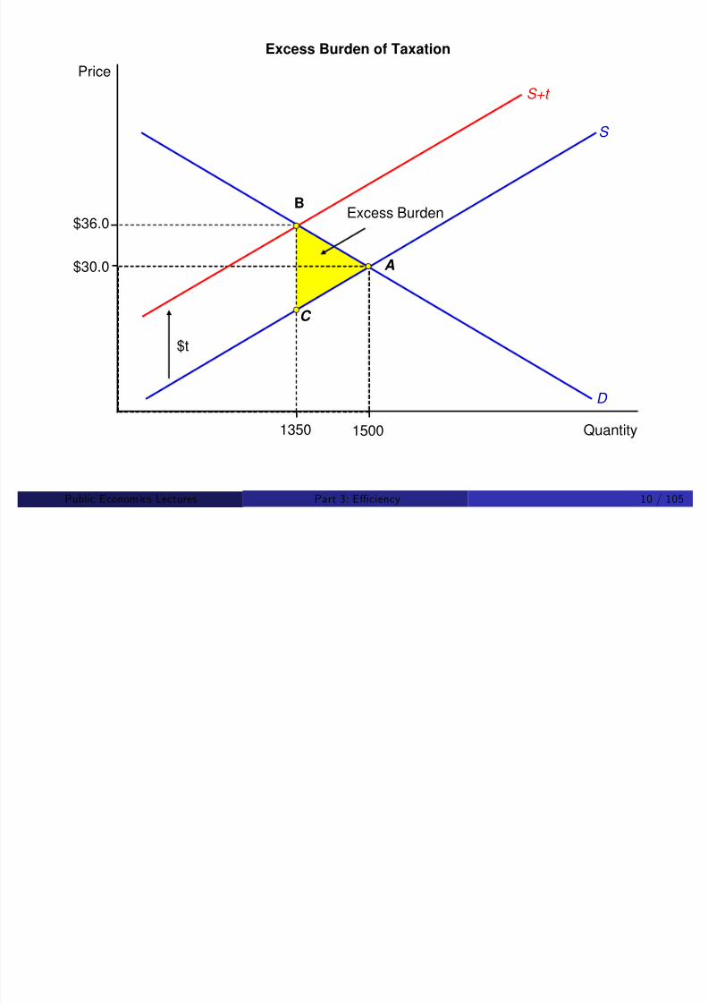
8/8/2019 Chetty - Public Economics Lectures
http://slidepdf.com/reader/full/chetty-public-economics-lectures 179/949
A
D
$36.0
$t
C
$30.0
15001350 Quantity
Public Econom ics Lectures () Part 3: E¢ciency 10 / 105
E¢ciency Cost: Marshallian Surplus
There are three empirically implementalbe ways to measure the area of the
triangle:

8/8/2019 Chetty - Public Economics Lectures
http://slidepdf.com/reader/full/chetty-public-economics-lectures 180/949
1 In terms of supply and demand elasticities
2 In terms of total change in equilibrium quantity caused by tax
3 In terms of change in government revenue
Public Econom ics Lectures () Part 3: E¢ciency 11 / 105
E¢ciency Cost: Marshallian Surplus
1. In terms of supply and demand elasticities:
EB =1
2dQd τ
EB =1
2S 0(p )dpd τ = (1/2)(pS 0/S )(S /p )ηD ηS ηD
d τ 2
EB =1 ηS ηD pQ(
d τ )2

8/8/2019 Chetty - Public Economics Lectures
http://slidepdf.com/reader/full/chetty-public-economics-lectures 181/949
EB =2 ηS ηD
pQ (p
)
Note: second line uses incidence formula dp = (ηD ηS ηD )d τ
Tax revenue R = Qd τ
Useful expression is deadweight burden per dollar of tax revenue:
EB
R =
1
2
ηS ηD ηS ηD
d τ
p
Public Econom ics Lectures () Part 3: E¢ciency 12 / 105

8/8/2019 Chetty - Public Economics Lectures
http://slidepdf.com/reader/full/chetty-public-economics-lectures 182/949
E¢ciency Cost: Marshallian Surplus
3. In terms of change in government revenue
Observe that with an initial tax rate of τ ,
EB =
1
2
ηS ηD ηS ηD pQ (
τ
p )2
Marginal excess burden (to a …rst-order approximation) is:

8/8/2019 Chetty - Public Economics Lectures
http://slidepdf.com/reader/full/chetty-public-economics-lectures 183/949
g ( pp )
∂EB
∂τ =
ηS ηD
ηS ηD Q τ
p = η
Q Q τ
p
First-order approx includes only loss in govt revenue due to behavioralresponse
Rectangle in the Harberger trapezoid, proportional to τ
Does not include the second-order term (proportional to τ 2)
Public Econom ics Lectures () Part 3: E¢ciency 14 / 105
E¢ciency Cost: Marshallian Surplus
Alternative representation for marginal excess burden can be obtainedusing data on government budget R (τ ) = Q τ
MEB equals the di¤erence between the “mechanical” revenue gainand the actual revenue gain
Mechanical revenue gain: ∂R jQ = Q

8/8/2019 Chetty - Public Economics Lectures
http://slidepdf.com/reader/full/chetty-public-economics-lectures 184/949
Mechanical revenue gain: ∂τ jQ = Q
Actual revenue gain: ∂R ∂τ = Q + τ dQ dp
Di¤erence between mechanical and actual revenue gain:
∂R
∂τ jQ
dR
d τ = Q [Q + τ
dQ
dp ] = τ
dQ
dp
= τ dQ dt p Q
Q p = τ p ηQ Q = ∂E ∂τ
Intuition: leakage in government revenue measures distortion
Public Econom ics Lectures () Part 3: E¢ciency 15 / 105
E¢ciency Cost: Qualitative Properties
EB =1
2
ηS ηD ηS ηD
pQ (d τ
p )2

8/8/2019 Chetty - Public Economics Lectures
http://slidepdf.com/reader/full/chetty-public-economics-lectures 185/949
1 Excess burden increases with square of tax rate
2 Excess burden increases with elasticities
Public Econom ics Lectures () Part 3: E¢ciency 16 / 105
P S
P
EB Increases with Square of Tax Rate
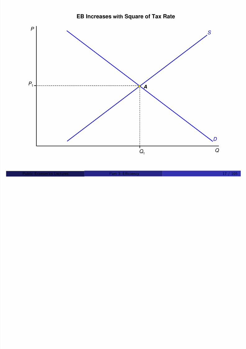
8/8/2019 Chetty - Public Economics Lectures
http://slidepdf.com/reader/full/chetty-public-economics-lectures 186/949
Q
D
A
Q 1
P 1
Public Econom ics Lectures () Part 3: E¢ciency 17 / 105
P S
S+t 1
B P 2
P
EB Increases with Square of Tax Rate

8/8/2019 Chetty - Public Economics Lectures
http://slidepdf.com/reader/full/chetty-public-economics-lectures 187/949
Q
D
A
C
Q 1Q 2
P 1
$t1
Public Econom ics Lectures () Part 3: E¢ciency 18 / 105
P S
S+t 1
B P 2
P
P 3E
S+t 1+t
2
Change in EB
EB Increases with Square of Tax Rate

8/8/2019 Chetty - Public Economics Lectures
http://slidepdf.com/reader/full/chetty-public-economics-lectures 188/949
Q
D
A
C
Q 1Q 2Q 3
P 1
D
$t2
Public Econom ics Lectures () Part 3: E¢ciency 19 / 105
(a) Inelastic Demand (b) Elastic Demand
P
S S+t
B P 2
P
S
S+t
B
Comparative Statics

8/8/2019 Chetty - Public Economics Lectures
http://slidepdf.com/reader/full/chetty-public-economics-lectures 189/949
P 2
P 1
Q 1Q 2Q
D
A
C $t
P 1
Q 1Q 2Q
D
A
C
$t
Public Econom ics Lectures () Part 3: E¢ciency 20 / 105
Tax Policy Implications
With many goods, formula suggests that the most e¢cient way toraise tax revenue is:

8/8/2019 Chetty - Public Economics Lectures
http://slidepdf.com/reader/full/chetty-public-economics-lectures 190/949
1 Tax relatively more the inelastic goods (e.g. medical drugs, food)
2 Spread taxes across all goods so as to keep tax rates relatively low onall goods (broad tax base)
Public Econom ics Lectures () Part 3: E¢ciency 21 / 105
General Model with Income E¤ects
Marshallian surplus is an ill-de…ned measure with income e¤ects
Drop quasilinearity assumption and consider an individual with utility
u (c 1, .., c N ) = u (c )

8/8/2019 Chetty - Public Economics Lectures
http://slidepdf.com/reader/full/chetty-public-economics-lectures 191/949
Individual program:
maxc
u (c ) s.t. q c Z
where q = p + t denotes vector of tax-inclusive prices and Z is wealth
Labor can be viewed as commodity with price w and consumed innegative quantity
Public Econom ics Lectures () Part 3: E¢ciency 22 / 105

8/8/2019 Chetty - Public Economics Lectures
http://slidepdf.com/reader/full/chetty-public-economics-lectures 192/949
Useful Properties of Demand and Utility
Multiplier on budget constraint λ = v Z is the marginal utility of wealth
Give wealth grant of dZ to consumer:
du = ∑ i
u c i dc i = λ∑ i
q i dc i = λdZ

8/8/2019 Chetty - Public Economics Lectures
http://slidepdf.com/reader/full/chetty-public-economics-lectures 193/949
i i
Roy’s identity: v q i = λc i
Welfare e¤ect of a price change dq i same as reducing wealth by:
dZ = c i dq i
By Envelope Thm., adjustment of c j does not produce a 1st orderwelfare e¤ect
Public Econom ics Lectures () Part 3: E¢ciency 24 / 105
Path Dependence Problem
Initial price vector q 0
Taxes levied on goods !price vector now q 1
Change in Marshallian surplus is de…ned as the line integral:
CS
Z q 1c(q Z )dq
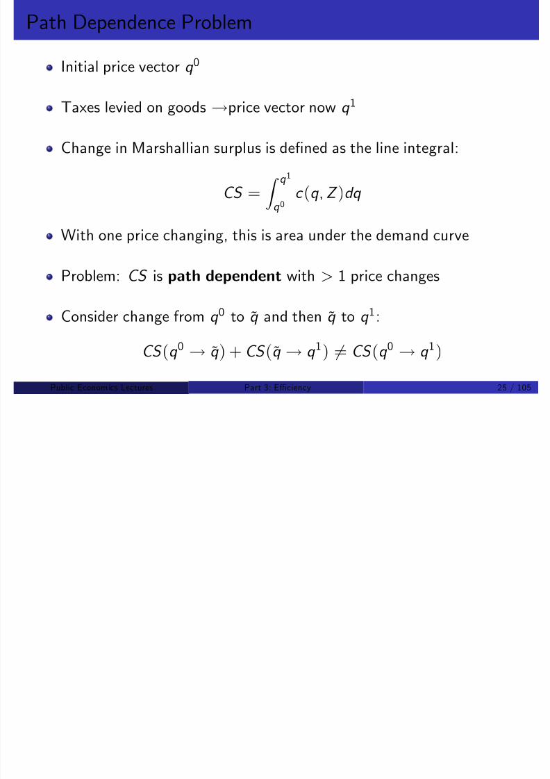
8/8/2019 Chetty - Public Economics Lectures
http://slidepdf.com/reader/full/chetty-public-economics-lectures 194/949
CS =Zq 0
c (q ,Z )dq
With one price changing, this is area under the demand curve
Problem: CS is path dependent with > 1 price changes
Consider change from q 0
to q and then q to q 1
:
CS (q 0 ! q ) + CS (q ! q 1) 6= CS (q 0 ! q 1)
Public Econom ics Lectures () Part 3: E¢ciency 25 / 105
Path Dependence Problem
Example of path dependence with taxes on two goods:
CS 1 =Z q 11q 01
c 1(q 1, q 02 , Z )dq 1 +Z q 12q 02
c 2(q 11 , q 2,Z )dq 2 (1)
CS
Z q 12( 0 Z )d +
Z q 11( 1 Z )d (2)

8/8/2019 Chetty - Public Economics Lectures
http://slidepdf.com/reader/full/chetty-public-economics-lectures 195/949
CS 2 =Zq 02
c 2(q 01 , q 2, Z )dq 2 +Zq 01
c 1(q 1, q 12 ,Z )dq 1 (2)
For CS 1 = CS 2, need dc 2dq 1
= dc 1dq 2
With income e¤ects, this symmetry condition is not satis…ed ingeneral
Public Econom ics Lectures () Part 3: E¢ciency 26 / 105
8/8/2019 Chetty - Public Economics Lectures
http://slidepdf.com/reader/full/chetty-public-economics-lectures 196/949
Expenditure Function
Fix utility at U and prices at q
Find bundle that minimizes cost to reach U for q :
e (q , U ) = minc
q c s.t. u (c ) U
Let µ denote multiplier on utility constraint
First order conditions given by:
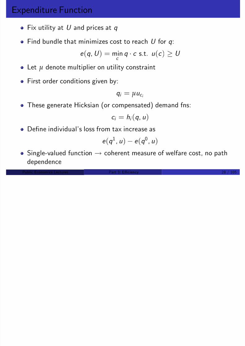
8/8/2019 Chetty - Public Economics Lectures
http://slidepdf.com/reader/full/chetty-public-economics-lectures 197/949
q i = µu c i
These generate Hicksian (or compensated) demand fns:
c i = hi (q , u )
De…ne individual’s loss from tax increase as
e (q 1
, u ) e (q 0
, u )Single-valued function ! coherent measure of welfare cost, no pathdependence
Public Econom ics Lectures () Part 3: E¢ciency 28 / 105
Compensating and Equivalent Variation
But where should u be measured?
Consider a price change from q 0 to q 1
Initial utility:

8/8/2019 Chetty - Public Economics Lectures
http://slidepdf.com/reader/full/chetty-public-economics-lectures 198/949
u 0 = v (q 0,Z )
Utility at new price q 1:u 1 = v (q 1,Z )
Two concepts: compensating (CV ) and equivalent variation (EV ) useu 0 and u 1 as reference utility levels
Public Econom ics Lectures () Part 3: E¢ciency 29 / 105
Compensating Variation
Measures utility at initial price level (u 0)
Amount agent must be compensated in order to be indi¤erent about
tax increase
CV = e (q 1, u 0) e (q 0, u 0) = e (q 1, u 0) Z
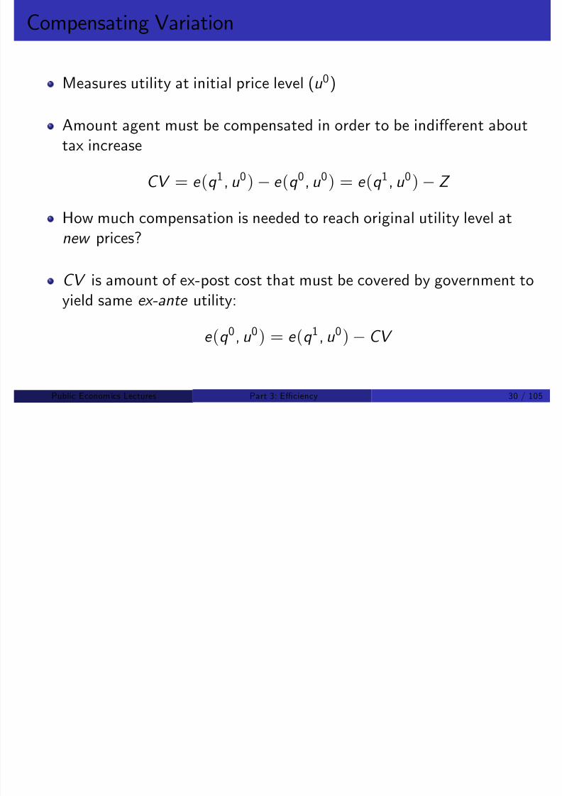
8/8/2019 Chetty - Public Economics Lectures
http://slidepdf.com/reader/full/chetty-public-economics-lectures 199/949
How much compensation is needed to reach original utility level at
new prices?
CV is amount of ex-post cost that must be covered by government toyield same ex-ante utility:
e (q 0, u 0) = e (q 1, u 0) CV
Public Econom ics Lectures () Part 3: E¢ciency 30 / 105
Equivalent Variation
Measures utility at new price level
Lump sum amount agent willing to pay to avoid tax (at pre-tax prices)
EV = e (q 1, u 1) e (q 0, u 1) = Z e (q 0, u 1)
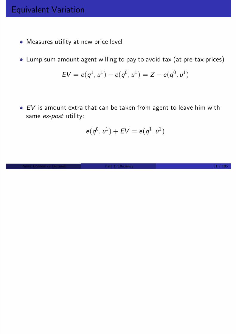
8/8/2019 Chetty - Public Economics Lectures
http://slidepdf.com/reader/full/chetty-public-economics-lectures 200/949
EV is amount extra that can be taken from agent to leave him withsame ex-post utility:
e (q 0, u 1) + EV = e (q 1, u 1)
Public Econom ics Lectures () Part 3: E¢ciency 31 / 105
E¢ciency Cost with Income E¤ects
Goal: derive empirically implementable formula analogous toMarshallian EB formula in general model with income e¤ects
Existing literature assumes either
1 Fixed producer prices and income e¤ectsE d d i d ili ili
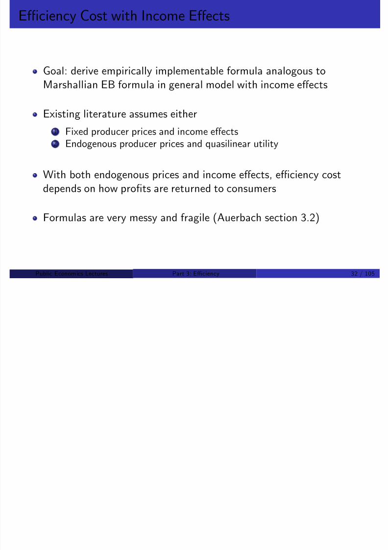
8/8/2019 Chetty - Public Economics Lectures
http://slidepdf.com/reader/full/chetty-public-economics-lectures 201/949
2 Endogenous producer prices and quasilinear utility
With both endogenous prices and income e¤ects, e¢ciency costdepends on how pro…ts are returned to consumers
Formulas are very messy and fragile (Auerbach section 3.2)
Public Econom ics Lectures () Part 3: E¢ciency 32 / 105
E¢ciency Cost Formulas with Income E¤ects
Derive empirically implementable formulas using Hicksian demand(EV and CV )
Assume p is …xed ! ‡at supply, constant returns to scale
The envelope thm implies that e q i (q , u ) = hi , and so:
q1
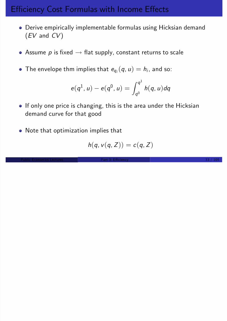
8/8/2019 Chetty - Public Economics Lectures
http://slidepdf.com/reader/full/chetty-public-economics-lectures 202/949
e (q 1, u ) e (q 0, u ) = Z q 1
q 0h(q , u )dq
If only one price is changing, this is the area under the Hicksiandemand curve for that good
Note that optimization implies that
h(q , v (q , Z )) = c (q ,Z )
Public Econom ics Lectures () Part 3: E¢ciency 33 / 105

8/8/2019 Chetty - Public Economics Lectures
http://slidepdf.com/reader/full/chetty-public-economics-lectures 203/949
Compensating vs. Equivalent Variation
p
p1
EV
h(V(p1,Z)) h(V(p0,Z))

8/8/2019 Chetty - Public Economics Lectures
http://slidepdf.com/reader/full/chetty-public-economics-lectures 204/949
p0
D
xx(p0,Z)x(p1,Z)
Public Econom ics Lectures () Part 3: E¢ciency 35 / 105
Compensating vs. Equivalent Variation
p
p1
CV
h(V(p1,Z)) h(V(p0,Z))

8/8/2019 Chetty - Public Economics Lectures
http://slidepdf.com/reader/full/chetty-public-economics-lectures 205/949
p0
D
xx(p0,Z)x(p1,Z)
Public Econom ics Lectures () Part 3: E¢ciency 36 / 105
Marshallian Surplus
p
p1
Marshallian Surplus
h(V(p1,Z)) h(V(p0,Z))

8/8/2019 Chetty - Public Economics Lectures
http://slidepdf.com/reader/full/chetty-public-economics-lectures 206/949
p0
D
xx(p0,Z)x(p1,Z)
Public Econom ics Lectures () Part 3: E¢ciency 37 / 105
Path Independence of EV, CV
With one price change:
EV < Marshallian Surplus < CV
but this is not true in general
No path dependence problem for EV, CV measures with multiple pricechanges

8/8/2019 Chetty - Public Economics Lectures
http://slidepdf.com/reader/full/chetty-public-economics-lectures 207/949
Slutsky equation:
∂hi ∂q j |{z}
Hicksian Slope
=∂c i ∂q j |{z}
Marshallian Slope
+ c j ∂c i ∂Z | {z }
Income E¤ect
Optimization implies Slutsky matrix is symmetric:∂h
i ∂q j =∂h j ∂q i
Therefore the integralR q 1q 0
h(q , u )dq is path independent
Public Econom ics Lectures () Part 3: E¢ciency 38 / 105
Excess Burden
Deadweight burden: change in consumer surplus less tax paid
Equals what is lost in excess of taxes paid
Two measures corresponding to EV and CV :

8/8/2019 Chetty - Public Economics Lectures
http://slidepdf.com/reader/full/chetty-public-economics-lectures 208/949
Two measures, corresponding to EV and CV :
EB (u 1) = EV (q 1 q 0)h(q 1, u 1) [Mohring 1971]
EB (u 0) = CV (q 1 q 0)h(q 1, u 0) [Diamond and McFadden 1974]
Public Econom ics Lectures () Part 3: E¢ciency 39 / 105
p
p
p1
EBCV
EBEV
h(V(p1,Z)) h(V(p0,Z))
~

8/8/2019 Chetty - Public Economics Lectures
http://slidepdf.com/reader/full/chetty-public-economics-lectures 209/949
p0
D
xx(p1,Z)~xC(p1,V(p0,Z))~~
Public Econom ics Lectures () Part 3: E¢ciency 40 / 105
p
p
p1
Marshallian
h(V(p1,Z)) h(V(p0,Z))
~

8/8/2019 Chetty - Public Economics Lectures
http://slidepdf.com/reader/full/chetty-public-economics-lectures 210/949
p0
D
xx(p1,Z)~xC(p1,V(p0,Z))~~
Public Econom ics Lectures () Part 3: E¢ciency 41 / 105
Excess Burden
In general, CV and EV measures of EB will di¤er
Marshallian measure overstates excess burden because it includesincome e¤ects
Income e¤ects are not a distortion in transactions

8/8/2019 Chetty - Public Economics Lectures
http://slidepdf.com/reader/full/chetty-public-economics-lectures 211/949
Buying less of a good due to having less income is not an e¢ciencyloss; no surplus foregone b/c of transactions that do not occur
Chipman and Moore (1980): CV = EV = Marshallian DWL only withquasilinear utility
Public Econom ics Lectures () Part 3: E¢ciency 42 / 105
Implementable Excess Burden Formula
Consider increase in tax τ on good 1 to τ + ∆τ
No other taxes in the system
Recall the expression for EB :
EB(τ) = [e(p + τ U) e(p U)] τh1(p + τ U)

8/8/2019 Chetty - Public Economics Lectures
http://slidepdf.com/reader/full/chetty-public-economics-lectures 212/949
EB (τ ) = [e (p + τ ,U ) e (p , U )] τ h1(p + τ , U )
Second-order Taylor expansion:
MEB = EB (τ + ∆τ ) EB (τ )
'dEB
d τ
(∆τ ) +1
2
(∆τ )2 d 2EB
d τ 2
Public Econom ics Lectures () Part 3: E¢ciency 43 / 105
Harberger Trapezoid Formula
dEB
d τ = h1(p + τ ,U ) τ
dh1
d τ h1(p + τ , U )
= τ dh1d τ
d 2EB
d τ 2=
dh1
d τ τ
d 2h1
d τ 2

8/8/2019 Chetty - Public Economics Lectures
http://slidepdf.com/reader/full/chetty-public-economics-lectures 213/949
Standard practice in literature: assume d 2h1d τ 2
(linear Hicksian); notnecessarily well justi…ed because it does not vanish as ∆τ ! 0
) MEB = τ ∆τ dh1
d τ
1
2
dh1
d τ (∆τ )2
Formula equals area of “Harberger trapezoid” using Hicksian demands
Public Econom ics Lectures () Part 3: E¢ciency 44 / 105
Harberger Formula
Without pre-existing tax, obtain “standard” Harberger formula:
EB = 1
2
dh1
d τ
(∆τ )2
Observe that …rst-order term vanishes when τ = 0
A new tax has second-order deadweight burden (proportional to ∆τ2

8/8/2019 Chetty - Public Economics Lectures
http://slidepdf.com/reader/full/chetty-public-economics-lectures 214/949
A new tax has second order deadweight burden (proportional to ∆τ
not ∆τ )
Bottom line: need compensated (substitution) elasticities to computeEB , not uncompensated elasticities
Empirically, need estimates of income and price elasticities
Public Econom ics Lectures () Part 3: E¢ciency 45 / 105
Excess Burden with Taxes on Multiple Goods
Previous formulas apply to case with tax on one good
With multiple goods and …xed prices, excess burden of introducing atax τ k
EB = 12τ 2k dhk d τ k
∑ i 6=k
τ i τ k dhi d τ k
Second-order e¤ect in own market, …rst-order e¤ect from othermarkets with pre-existing taxes
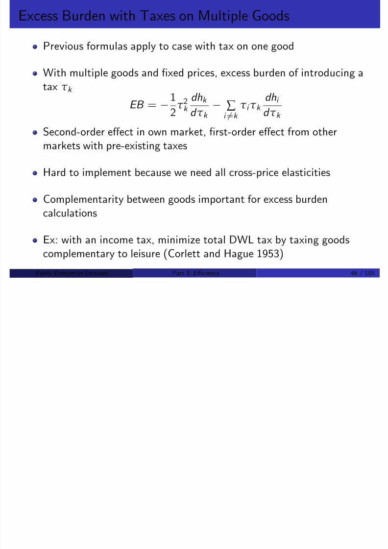
8/8/2019 Chetty - Public Economics Lectures
http://slidepdf.com/reader/full/chetty-public-economics-lectures 215/949
p g
Hard to implement because we need all cross-price elasticities
Complementarity between goods important for excess burdencalculations
Ex: with an income tax, minimize total DWL tax by taxing goodscomplementary to leisure (Corlett and Hague 1953)
Public Econom ics Lectures () Part 3: E¢ciency 46 / 105
Goulder and Williams 2003
Show that ignoring cross e¤ects by using one-good formula can bevery misleading
Di¤erentiate multiple-good Harberger formula w.r.t. τ k :
dEB
dτk= τ k
dhk
dτk ∑
6τ i
dhi
dτk

8/8/2019 Chetty - Public Economics Lectures
http://slidepdf.com/reader/full/chetty-public-economics-lectures 216/949
d τ k d τ k i 6=k d τ k
If τ k is small (e.g. gas tax), what matters is purely distortion in othermarkets, e.g. labor supply
As τ k ! 0, error in single-market formula approaches ∞
Public Econom ics Lectures () Part 3: E¢ciency 47 / 105
Goulder and Williams: Assumptions
Make multiple-goods formula empirically implementable by making 3
assumptions/approximations:
1 No income e¤ects
2 Ignore interactions with commodities other than labor (other taxes are
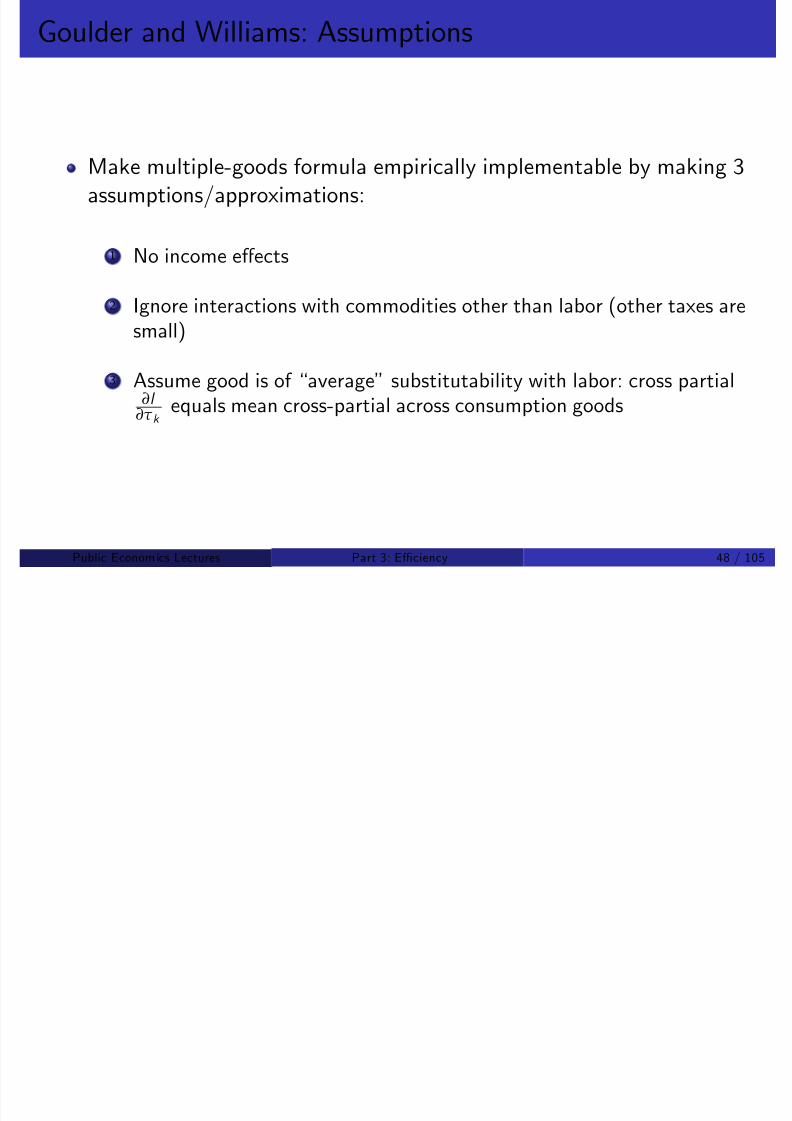
8/8/2019 Chetty - Public Economics Lectures
http://slidepdf.com/reader/full/chetty-public-economics-lectures 217/949
2 Ignore interactions with commodities other than labor (other taxes are
small)
3 Assume good is of “average” substitutability with labor: cross partial∂l ∂τ k
equals mean cross-partial across consumption goods
Public Econom ics Lectures () Part 3: E¢ciency 48 / 105
Goulder and Williams Formula
Obtain following formula for marginal excess burden of raising tax ongood k :
dEB
d τ k =
τ k Q k p k
ηk τ LL
p k ηLs k
τ k , p k , and Q k are the tax, price, and quantity consumed of good k ηk and ηL are own-price elasticity of good k and labor
s k = P k Q K wl (1τ L) is budget share of good k
O l d i f i l i i i i l hi

8/8/2019 Chetty - Public Economics Lectures
http://slidepdf.com/reader/full/chetty-public-economics-lectures 218/949
Only need estimates of own-price elasticities to implement this
formula
Why? Price increase in all consumption goods has the same e¤ect onlabor supply as an increase in tax on labor:
(1 + t )∑ k p k c k = wl
Equivalence between consumption tax and labor income tax
Public Econom ics Lectures () Part 3: E¢ciency 49 / 105
Goulder and Williams Formula
Rank goods according to complementarity with labor (i.e.cross-partial dl
d τ k )
Find good at the mean level of dl d τ k
A tax increase on this good has same e¤ect as an increase in sales taxt on all consumption goods scaled down by s k

8/8/2019 Chetty - Public Economics Lectures
http://slidepdf.com/reader/full/chetty-public-economics-lectures 219/949
p g y k
Therefore cross-elasticity is equivalent to labor-supply elasticity timess k
Labor supply elasticity ηL su¢cient to calculate cross-elasticity for
good that has “average” level of substitutability
Public Econom ics Lectures () Part 3: E¢ciency 50 / 105
Goulder and Williams Results
Calibrate formula using existing elasticity estimates
Result: DWL of taxing goods such as gasoline is underestimated by afactor of 10 in practice because of income tax
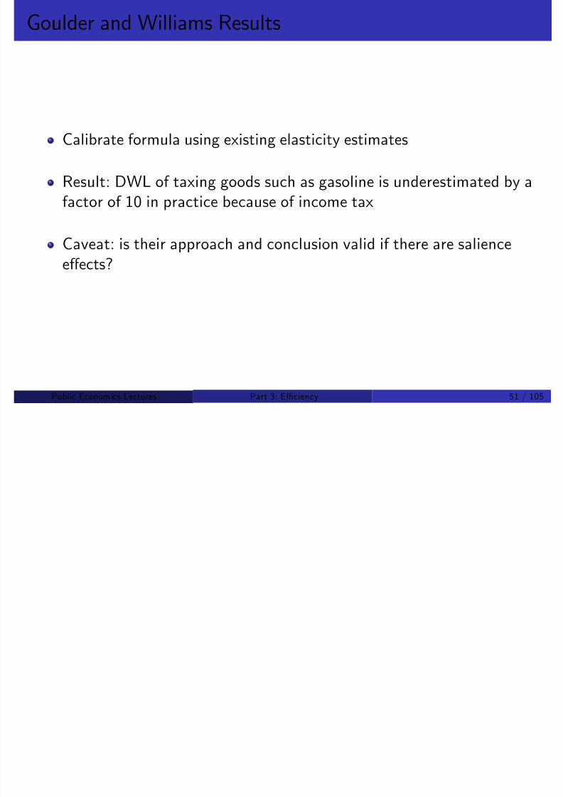
8/8/2019 Chetty - Public Economics Lectures
http://slidepdf.com/reader/full/chetty-public-economics-lectures 220/949
Caveat: is their approach and conclusion valid if there are saliencee¤ects?
Public Econom ics Lectures () Part 3: E¢ciency 51 / 105
Hausman 1981: Exact Consumer Surplus
Harberger formulas: empirically implementable, but approximations(linearity, ignore cross-e¤ects)
Alternative approach: full structural estimation of demand model
Start from observed market demand functions, …nding the best …t
Estimate regression of the form:
c(q Z ) γ + αq + δZ

8/8/2019 Chetty - Public Economics Lectures
http://slidepdf.com/reader/full/chetty-public-economics-lectures 221/949
c (q ,Z ) = γ + αq + δZ
Then integrate to recover underlying indirect utility function v (q ,Z )
Inverting yields expenditure function e (q , u ); now compute “exact”EB
Parametric approach: Hausman (AER 1981); non-parametricapproach: Hausman and Newey (ECMA 1995)
Public Econom ics Lectures () Part 3: E¢ciency 52 / 105
8/8/2019 Chetty - Public Economics Lectures
http://slidepdf.com/reader/full/chetty-public-economics-lectures 222/949
Su¢cient Statistics vs Structural Methods
N goods: x = (x 1, ..., x N ); Prices: (p 1, ...p N ); Z = wealth
Normalize p N = 1 (x N is numeraire)
Government levies a tax t on good 1
Individual takes t as given and solves
max u (x 1, ..., x N 1) + x N s.t. (p 1 + t )x 1 +N
∑ i 2
p i x i = Z
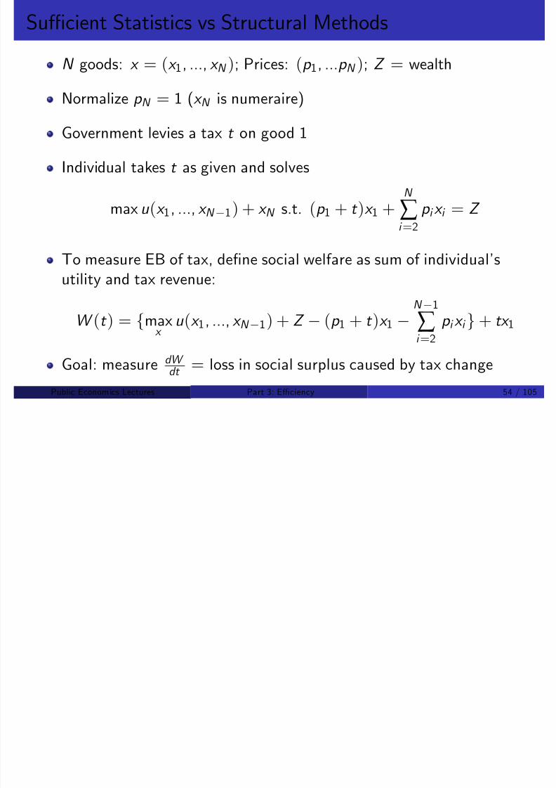
8/8/2019 Chetty - Public Economics Lectures
http://slidepdf.com/reader/full/chetty-public-economics-lectures 223/949
i =2
To measure EB of tax, de…ne social welfare as sum of individual’sutility and tax revenue:
W (t ) = fmaxx
u (x 1, ..., x N 1) + Z (p 1 + t )x 1 N 1
∑ i =2
p i x i g + tx 1
Goal: measure dW dt
= loss in social surplus caused by tax change
Public Econom ics Lectures () Part 3: E¢ciency 54 / 105
K1Ýt Þ
K2Ýt Þ
ω=preferences, β = f(ω,t) dW/dt used forconstraints y β X + β X + ε policy analysis
ω1
ω2
.
.
.ωΝ
dW
dt Ýt Þ
Primitives Sufficient Stats. Welfare Change

8/8/2019 Chetty - Public Economics Lectures
http://slidepdf.com/reader/full/chetty-public-economics-lectures 224/949
constraints y = β1X1 + β2X2 + ε policy analysis
ω not uniquely β identified usingidentified program evaluation
Source: Chetty (2009)
Public Econom ics Lectures () Part 3: E¢ciency 55 / 105
Su¢cient Statistics vs Structural Methods
Structural method: estimate N good demand system, recover u
Ex: use Stone-Geary or AIDS to recover preference parameters; thencalculate “exact consumer surplus” as in Hausman (1981)
Alternative: Harberger’s deadweight loss triangle formula
Private sector choices made to maximize term in red (private surplus)
W ( ) f ( ) Z ( )N 1
g

8/8/2019 Chetty - Public Economics Lectures
http://slidepdf.com/reader/full/chetty-public-economics-lectures 225/949
W (t ) = fmaxx
u (x 1
, ..., x N 1
) + Z (p 1
+ t )x 1
∑ i =2
p i x i g + tx 1
Envelope conditions for (x 1, ..., x N ) allow us to ignore behavioral
responses (dx i dt ) in term in red, yielding
dW
dt = x 1 + x 1 + t
dx 1
dt = t
dx 1
dt
! dx 1dt is a “su¢cient statistic” for calculating dW
dt
Public Econom ics Lectures () Part 3: E¢ciency 56 / 105
Heterogeneity
Bene…t of su¤ stat approach particularly evident with heterogeneity
K agents, each with utility u k (x 1 , ..., x N 1) + x N
Social welfare function under utilitarian criterion:
W (t ) = fmaxx
K
∑ k =1
[u k (x k 1 , ..., x k N 1) + Z
(p 1 + t )x k 1 N 1
∑ p i x k i ]g +K
∑ tx k 1

8/8/2019 Chetty - Public Economics Lectures
http://slidepdf.com/reader/full/chetty-public-economics-lectures 226/949
i =2 k =1
Structural method: estimate demand systems for all agents
Su¢cient statistic formula is unchanged—still need only slope of aggregate demand dx 1
dt
dW dt
= K ∑ k =1
x k 1 + K ∑ k =1
x k 1 + t d ∑ K k =1 x k 1
dt = t dx 1
dt
Public Econom ics Lectures () Part 3: E¢ciency 57 / 105
Discrete Choice Model
Two good model
Agents have value V k for good 1; can either buy or not buy
Let F (V ) denote distribution of valuations
Utility of agent k is
V k x 1 + Z (p + t )x 1
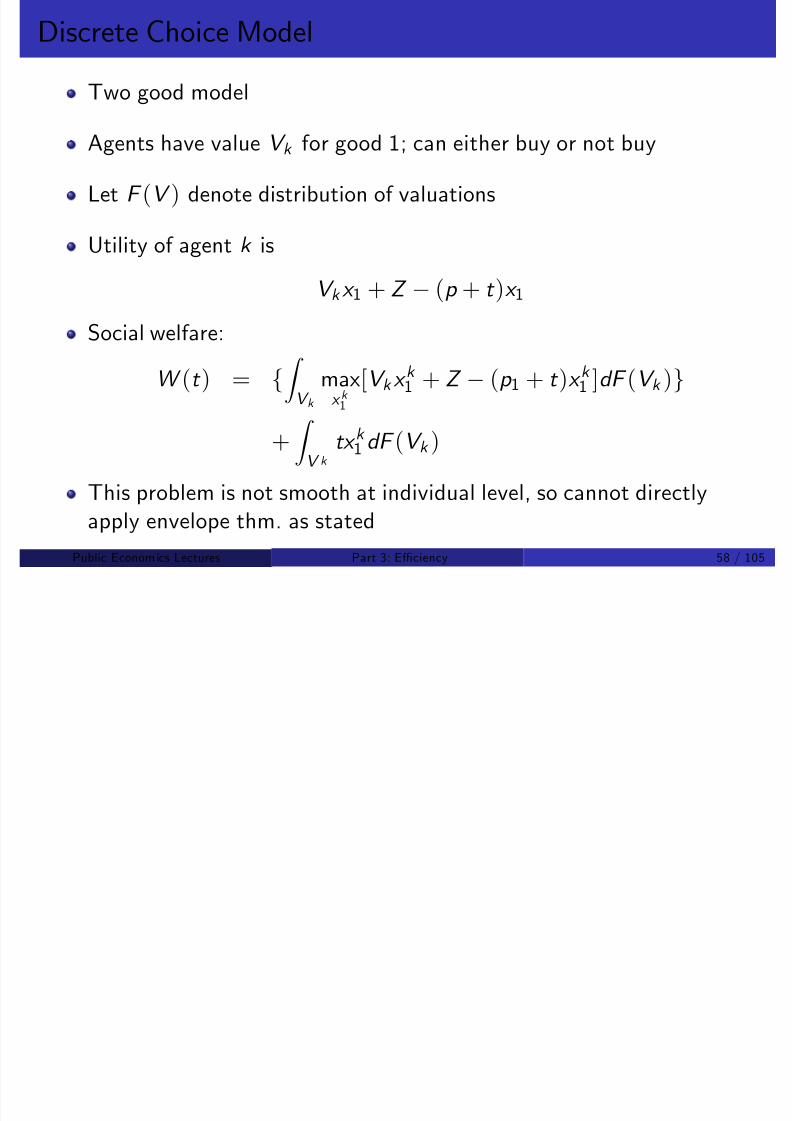
8/8/2019 Chetty - Public Economics Lectures
http://slidepdf.com/reader/full/chetty-public-economics-lectures 227/949
Social welfare:W (t ) = f
Z V k
maxx k 1
[V k x k 1 + Z (p 1 + t )x k 1 ]dF (V k )g
+ Z V k tx k 1 dF (V k )
This problem is not smooth at individual level, so cannot directlyapply envelope thm. as stated
Public Econom ics Lectures () Part 3: E¢ciency 58 / 105
Discrete Choice Model
Recast as planner’s problem choosing threshold above which agentsare allocated good 1:
W (t ) = (max_V
Z ∞_V [V k (p 1 + t )] dF (V k ) + Z )
+t
Z ∞_
V dF (V k )
A ai obtai Ha be e fo la as a f of slo e of a e ate de a d
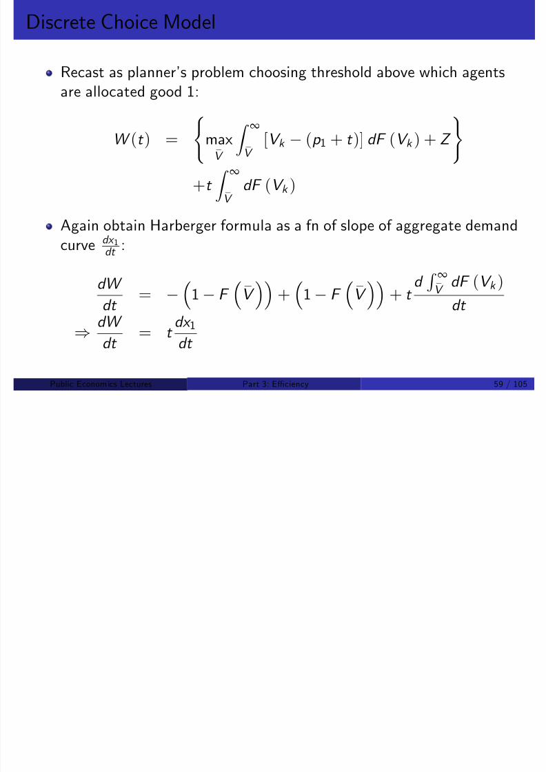
8/8/2019 Chetty - Public Economics Lectures
http://slidepdf.com/reader/full/chetty-public-economics-lectures 228/949
Again obtain Harberger formula as a fn of slope of aggregate demandcurve dx 1
dt :
dW
dt =
1 F
_
V
+
1 F
_
V
+ t
d R ∞_V
dF (V k )
dt
) dW dt
= t dx 1dt
Public Econom ics Lectures () Part 3: E¢ciency 59 / 105
Economic Intuition for Robustness of Harberger Result
Deadweight loss is fully determined by di¤erence between marginalwillingness to pay for good x 1 and its cost (p 1)
Recovering marginal willingness to pay requires an estimate of theslope of the demand curve because it coincides with marginal utility:
p = u 0(x (p ))

8/8/2019 Chetty - Public Economics Lectures
http://slidepdf.com/reader/full/chetty-public-economics-lectures 229/949
Slope of demand is therefore su¢cient to infer e¢ciency cost of a tax,without identifying rest of the model
Public Econom ics Lectures () Part 3: E¢ciency 60 / 105
E¢ciency Cost: Applications
1 [Income Taxation] Feldstein; Chetty; Gorodnichenko et al.
2 [Housing Subsidy] Poterba

8/8/2019 Chetty - Public Economics Lectures
http://slidepdf.com/reader/full/chetty-public-economics-lectures 230/949
3 [Diesel Fuel Taxation] Marion and Muehlegger
Public Econom ics Lectures () Part 3: E¢ciency 61 / 105
Feldstein 1995, 1999
Following Harberger, large literature in labor estimated e¤ect of taxeson hours worked to assess e¢ciency costs of taxation
Feldstein observed that labor supply involves multiple dimensions, not just choice of hours: training, e¤ort, occupation
Taxes also induce ine¢cient avoidance/evasion behavior
8/8/2019 Chetty - Public Economics Lectures
http://slidepdf.com/reader/full/chetty-public-economics-lectures 231/949
Structural approach: account for each of the potential responses totaxation separately and then aggregate
Feldstein’s alternative: elasticity of taxable income with respect to
taxes is a su¢cient statistic for calculating deadweight loss
Public Econom ics Lectures () Part 3: E¢ciency 62 / 105
Feldstein Model: Setup
Government levies linear tax t on reported taxable income
Agent makes N labor supply choices: l 1, ...l N
Each choice l i has disutility ψi (l i ) and wage w i
Agents can shelter $e of income from taxation by paying cost g (e )
Taxable Income (TI ) is

8/8/2019 Chetty - Public Economics Lectures
http://slidepdf.com/reader/full/chetty-public-economics-lectures 232/949
Taxable Income (TI ) is
TI =N
∑ i =1
w i l i e
Consumption is given by taxed income plus untaxed income:
c = (1 t )TI + e
Public Econom ics Lectures () Part 3: E¢ciency 63 / 105
Feldstein Taxable Income Formula
Agent’s utility is quasi-linear in consumption:
u (c , e , l ) = c g (e ) N
∑ i =1
ψi (l i )
Social welfare:
W (t ) = f(1 t )TI + e g (e ) N
∑ i =1
ψi (l i )g + tTI

8/8/2019 Chetty - Public Economics Lectures
http://slidepdf.com/reader/full/chetty-public-economics-lectures 233/949
Di¤erentiating and applying envelope conditions for l i ((1 t )w i = ψ0
i (l i )) and e (g 0(e ) = t ) implies
dW
dt = TI + TI t
dTI
dt = t
dTI
dt
Intuition: marginal social cost of reducing earnings through eachmargin is equated at optimum ! irrelevant what causes change in TI
Public Econom ics Lectures () Part 3: E¢ciency 64 / 105
Taxable Income Formula
Simplicity of identi…cation in Feldstein’s formula has led to a largeliterature estimating elasticity of taxable income
But since primitives are not estimated, assumptions of model used toderive formula are never tested
Chetty (2009) questions validity of assumption that g 0(e ) = t

8/8/2019 Chetty - Public Economics Lectures
http://slidepdf.com/reader/full/chetty-public-economics-lectures 234/949
Costs of some avoidance/evasion behaviors are transfers to otheragents in the economy, not real resource costs
Ex: cost of evasion is potential …ne imposed by government
Public Econom ics Lectures () Part 3: E¢ciency 65 / 105
Chetty Transfer Cost Model: Setup
Individual chooses e (evasion/shifting) and l (labor supply) to
maxe ,
l
u (c , l , e ) = c ψ(l )
s.t. c = y + (1 t )(wl e ) + e z (e )
Social welfare is now:

8/8/2019 Chetty - Public Economics Lectures
http://slidepdf.com/reader/full/chetty-public-economics-lectures 235/949
W (t ) = fy + (1 t )(wl e ) + e z (e ) ψ(l )g
+z (e ) + t (wl e )
Di¤erence: z (e ) now appears twice in SWF, with opposite signs
Public Econom ics Lectures () Part 3: E¢ciency 66 / 105
Excess Burden with Transfer Costs
Let LI = wl be the total (pretax) earned income and TI = wl e
denote taxable income
Exploit the envelope condition for term in curly brackets:
dW dt
= (wl e ) + (wl e ) + dz de
de dt
+ t d [wl e ]dt
= t dTI
dt +
dz
de
de
dt
= t dLI
t de
+dz de

8/8/2019 Chetty - Public Economics Lectures
http://slidepdf.com/reader/full/chetty-public-economics-lectures 236/949
dt dt +
de dt First-order condition for individual’s choice of e :
t =dz
de
)dW
dt = t
dLI
dt (1)
Intuition: MPB of raising e by $1 (saving $t ) equals MPC
Public Econom ics Lectures () Part 3: E¢ciency 67 / 105
Chetty (2009) Formula
With both transfer cost z (e ) and resource cost g (e ) of evasion:
dW
dt = t
dLI
dt g 0(e )
de
dt
= t fµdTI
dt + (1 µ)
dLI
dt g
= t
1 t fµTI εTI + (1 µ)wl εLI g

8/8/2019 Chetty - Public Economics Lectures
http://slidepdf.com/reader/full/chetty-public-economics-lectures 237/949
EB depends on weighted average of taxable income (εTI ) and totalearned income elasticities (εLI )
Practical importance: even though reported taxable income is highlysensitive to tax rates for rich, e¢ciency cost may not be large!
Most di¢cult parameter to identify: weight µ, which depends onmarginal resource cost of sheltering, g 0(e )
Public Econom ics Lectures () Part 3: E¢ciency 68 / 105
Gorodnichenko, Martinez-Vazquez, and Peter 2009
Estimate εLI and εTI to implement formula that permits transfer costs
Insight: consumption data can be used to infer εLI
Estimate e¤ect of 2001 ‡at tax reform in Russia on gap between

8/8/2019 Chetty - Public Economics Lectures
http://slidepdf.com/reader/full/chetty-public-economics-lectures 238/949
taxable income and consumption, which they interpret as evasion
Public Econom ics Lectures () Part 3: E¢ciency 69 / 105
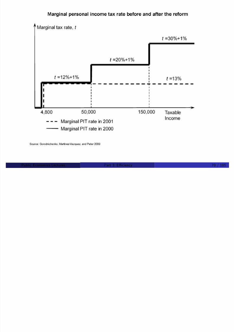
8/8/2019 Chetty - Public Economics Lectures
http://slidepdf.com/reader/full/chetty-public-economics-lectures 239/949
Public Econom ics Lectures () Part 3: E¢ciency 70 / 105

8/8/2019 Chetty - Public Economics Lectures
http://slidepdf.com/reader/full/chetty-public-economics-lectures 240/949
Gorodnichenko et al: Results
Taxable income elasticity dTI
dt
is large, whereas labor income elasticitydLI dt
is not
! Feldstein’s formula overestimates the e¢ciency costs of taxationrelative to more general measure for “plausible” g 0(e )
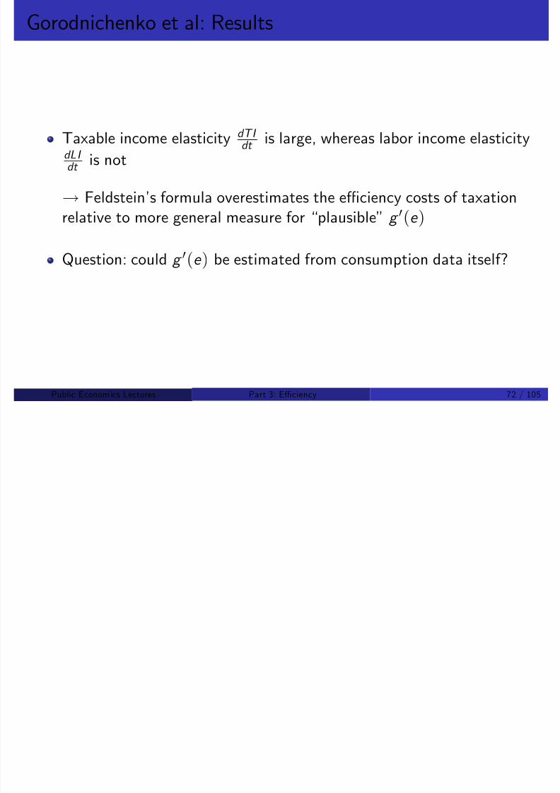
8/8/2019 Chetty - Public Economics Lectures
http://slidepdf.com/reader/full/chetty-public-economics-lectures 241/949
Question: could g 0(e ) be estimated from consumption data itself?
Public Econom ics Lectures () Part 3: E¢ciency 72 / 105

8/8/2019 Chetty - Public Economics Lectures
http://slidepdf.com/reader/full/chetty-public-economics-lectures 242/949
Porterba 1992
Poterba …rst calculates changes in user cost over 1980s
Tax reform in 1986 lowered tax rates for high income and raised usercost of housing sharply
Prior to 1986: very high tax rates on high incomes (60%)

8/8/2019 Chetty - Public Economics Lectures
http://slidepdf.com/reader/full/chetty-public-economics-lectures 243/949
In 1990, only 28%
Nearly tripled the cost of housing
Public Econom ics Lectures () Part 3: E¢ciency 74 / 105
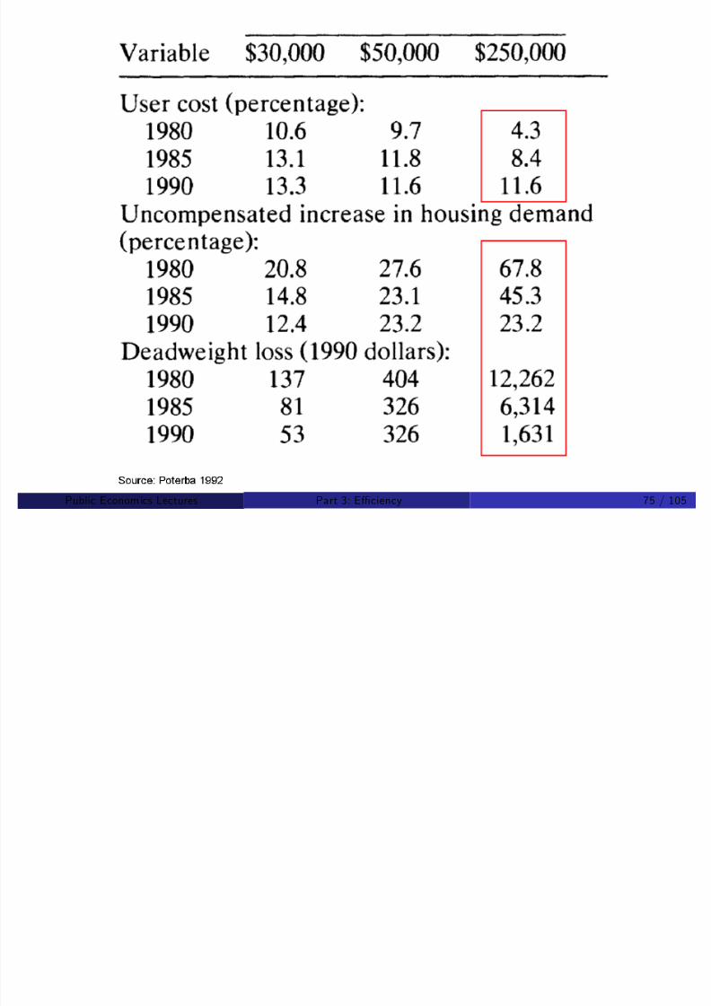
8/8/2019 Chetty - Public Economics Lectures
http://slidepdf.com/reader/full/chetty-public-economics-lectures 244/949
Porterba 1992
Calculates compensated elasticity using estimates in literature andSlutsky eqn.
Rosen (1982): εH ,r = 1
Income elasticity: 0.75Housing share: 0.25
) Compensated elasticity: 1 +3
4
1
4' 0.8
I f l l b k l l “h h h
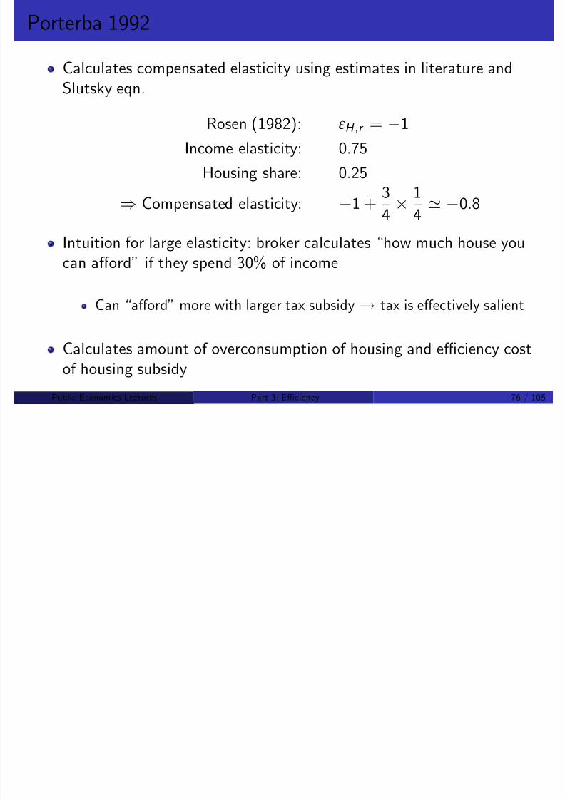
8/8/2019 Chetty - Public Economics Lectures
http://slidepdf.com/reader/full/chetty-public-economics-lectures 245/949
Intuition for large elasticity: broker calculates “how much house youcan a¤ord” if they spend 30% of income
Can “a¤ord” more with larger tax subsidy ! tax is e¤ectively salient
Calculates amount of overconsumption of housing and e¢ciency costof housing subsidy
Public Econom ics Lectures () Part 3: E¢ciency 76 / 105
Porterba: Results
Tax reforms in 1980s reduced DWL from $12K to $2K for eachhousehold earning $250K
Still have relatively large ine¢ciency from subsidizing mortgages
This is why President Bush’s Tax Panel recommended cap or
li i i f b id f h hi
8/8/2019 Chetty - Public Economics Lectures
http://slidepdf.com/reader/full/chetty-public-economics-lectures 246/949
elimination of subsidy for homeownership
But hard to implement politically
Public Econom ics Lectures () Part 3: E¢ciency 77 / 105
Marion and Muehlegger 2008
Study deadweight cost from taxing diesel fuels, focusing on evasion
Diesel fuel used for business purposes (e.g. trucking) is taxed, but
residential purposes (e.g. heating homes) is not
Substantial opportunity to evade tax
1993 dd d d d id i l di l f l

8/8/2019 Chetty - Public Economics Lectures
http://slidepdf.com/reader/full/chetty-public-economics-lectures 247/949
1993: government added red dye to residential diesel fuel
Easy to monitor cheating by opening gas tank of a truck
First document e¤ect of dye reform on evasion
Public Econom ics Lectures () Part 3: E¢ciency 78 / 105
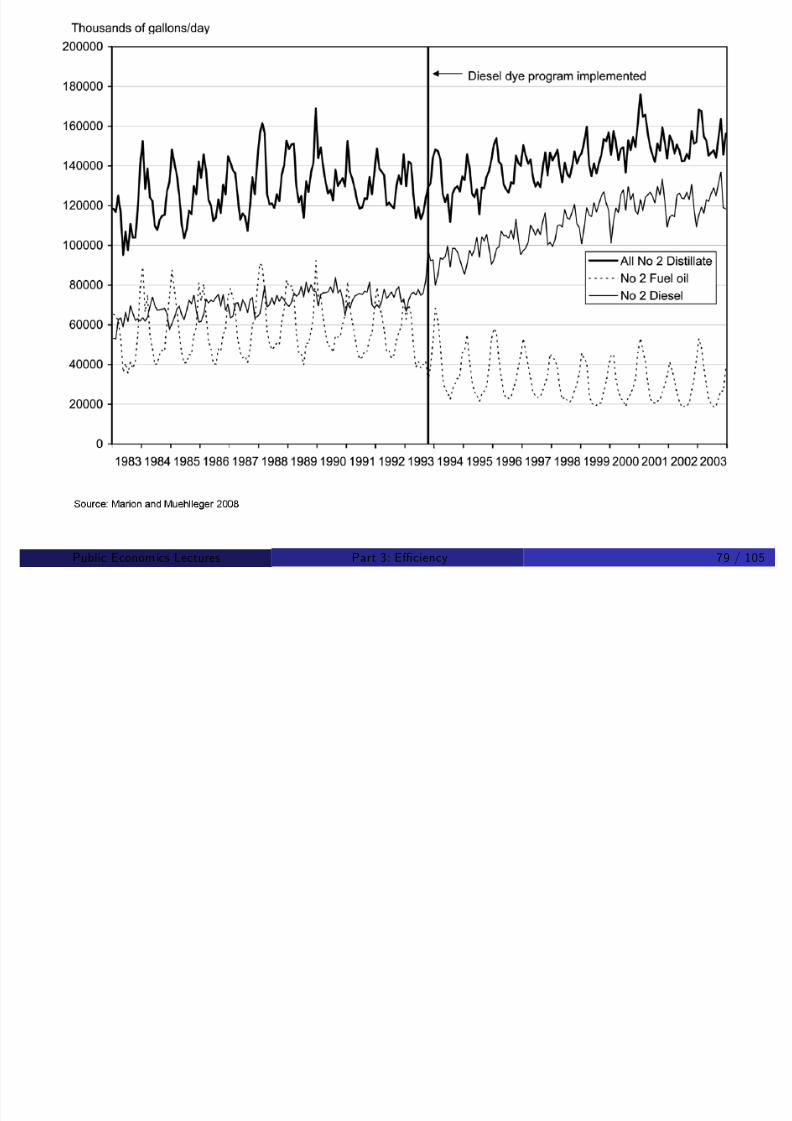
8/8/2019 Chetty - Public Economics Lectures
http://slidepdf.com/reader/full/chetty-public-economics-lectures 248/949
Public Econom ics Lectures () Part 3: E¢ciency 79 / 105
Marion and Muehlegger: Excess Burden Calculations
Use reform to assess deadweight costs of evasion and taxation
Harder to evade ! elasticity of behavior with respect to tax is muchlower after reform
Estimate price and tax elasticities before and after reform
U t t i ti i t t d i i ti f ld

8/8/2019 Chetty - Public Economics Lectures
http://slidepdf.com/reader/full/chetty-public-economics-lectures 249/949
Use cross-state variation in tax rates and price variation from worldmarket
Note di¤erent interpretation of di¤erence between price and taxelasticities in this study relative to tax salience papers
Public Econom ics Lectures () Part 3: E¢ciency 80 / 105
Price and Tax Elasticities By Year

8/8/2019 Chetty - Public Economics Lectures
http://slidepdf.com/reader/full/chetty-public-economics-lectures 250/949
Public Econom ics Lectures () Part 3: E¢ciency 81 / 105
Marion and Muehlegger: Results
Elasticities imply that 1% increase in tax rate raised revenue by0.60% before dye reform vs. 0.71% after reform
Reform reduced deadweight cost of diesel taxation
MDWL = 40 cents per dollar of revenue raised before dye reform
MDWL = 30 cents per dollar after reform

8/8/2019 Chetty - Public Economics Lectures
http://slidepdf.com/reader/full/chetty-public-economics-lectures 251/949
Lesson: Deadweight cost depends not just on preferences but also onenforcement technology
But again need to think carefully about marginal costs of evasion inthis context: social or transfer?
Public Econom ics Lectures () Part 3: E¢ciency 82 / 105
8/8/2019 Chetty - Public Economics Lectures
http://slidepdf.com/reader/full/chetty-public-economics-lectures 252/949
Behavioral Welfare Economics
Abstractly, e¤ect of policies on welfare are calculated in two steps
1 E¤ect of policy on behavior
2 E¤ect of change in behavior on utility
Challenge: identifying (2) when agents do not optimize perfectly
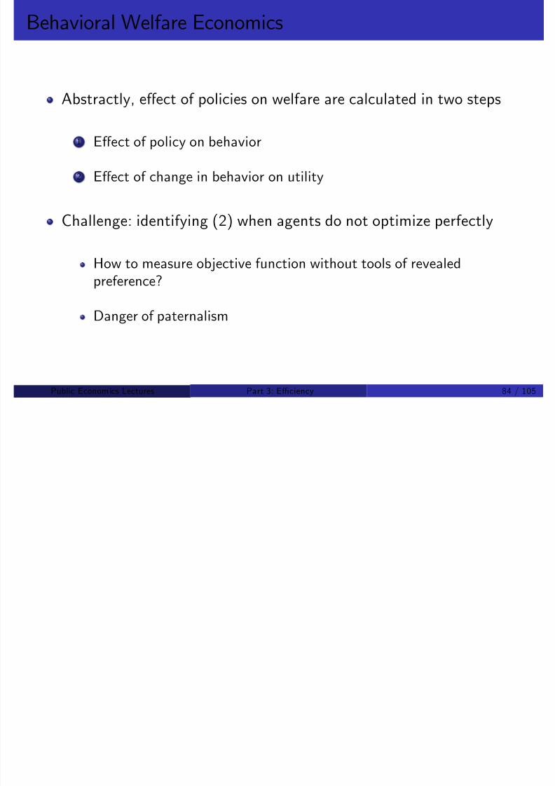
8/8/2019 Chetty - Public Economics Lectures
http://slidepdf.com/reader/full/chetty-public-economics-lectures 253/949
How to measure objective function without tools of revealedpreference?
Danger of paternalism
Public Econom ics Lectures () Part 3: E¢ciency 84 / 105
Behavioral Welfare Economics: Two Approaches
Approach #1: Build a positive model of deviations from rationality
Ex: hyperbolic discounting, bounded rationality, reference dependence
Then calculate optimal policy within such models
Approach #2: Choice-theoretic welfare analysis (Bernheim andRangel 2009)

8/8/2019 Chetty - Public Economics Lectures
http://slidepdf.com/reader/full/chetty-public-economics-lectures 254/949
Do not specify a positive model to rationalize behavior
Instead map directly from observed choices to statements about welfare
Analogous to “su¢cient statistic” approach
Public Econom ics Lectures () Part 3: E¢ciency 85 / 105
Behavioral Welfare Economics: Two Approaches
Consider three di¤erent medicare plans with di¤erent copays: L,M ,H
and corresponding variation in premiums
We have data from two environments:
1 On red paper, H > M > L

8/8/2019 Chetty - Public Economics Lectures
http://slidepdf.com/reader/full/chetty-public-economics-lectures 255/949
2 On blue paper, M > H > L
Public Econom ics Lectures () Part 3: E¢ciency 86 / 105
Behavioral Welfare Economics: Two Approaches
Approach 1: build a model of why color a¤ects choice and use it topredict which choice reveals “true” experienced utility
Approach 2: Yields bounds on optimal policy
L cannot be optimal given available data irrespective of positive
Optimal copay bounded between M and H

8/8/2019 Chetty - Public Economics Lectures
http://slidepdf.com/reader/full/chetty-public-economics-lectures 256/949
Optimal copay bounded between M and H
Key insight: no theory of choice needed to make statements aboutwelfare (do not need to understand why color a¤ects choice).
Public Econom ics Lectures () Part 3: E¢ciency 87 / 105
Bernheim and Rangel 2009: Setup
Theory that delivers bounds on welfare based purely on choice data
In standard model, agents choose from a choice set x 2 X
Goal of policy is to identify optimal x
In behavioral models, agents choose from “generalized choice sets”G = (X , d )

8/8/2019 Chetty - Public Economics Lectures
http://slidepdf.com/reader/full/chetty-public-economics-lectures 257/949
d is an “ancillary condition” – something that a¤ects choice behaviorbut (by assumption) does not a¤ect experienced utility
Ex: color of paper, salience, framing, default option
Public Econom ics Lectures () Part 3: E¢ciency 88 / 105
Bernheim and Rangel 2009: Choice Sets
Let C (X , d ) denote choice made in a given GCS
Choice inconsistency if C
(X , d
) 6=C
(X , d 0
)
De…ne revealed preference relation P as xPy if x always chosen overy for any d
Using P, can identify choice set that maximizes welfare instead of

8/8/2019 Chetty - Public Economics Lectures
http://slidepdf.com/reader/full/chetty-public-economics-lectures 258/949
Using P , can identify choice set that maximizes welfare instead of single point
With continuous choices, e¤ectively obtain bounds on welfare
Public Econom ics Lectures () Part 3: E¢ciency 89 / 105
Bernheim and Rangel 2009: Compensating Variation
Consider a change in choice set from X to X 0 X
Compute CV as amount needed to make agent indi¤erent to restrictionof choice set for each d (standard calculation)
Lower bound on CV is minimum over all d ’s
Upper bound on CV is maximum over all d ’s

8/8/2019 Chetty - Public Economics Lectures
http://slidepdf.com/reader/full/chetty-public-economics-lectures 259/949
Upper bound on CV is maximum over all d s
Public Econom ics Lectures () Part 3: E¢ciency 90 / 105
Bernheim and Rangel 2009: Compensating Variation
Ex: suppose insurance plans are restricted to drop M option
Under red paper condition, CV is 0 – no loss in welfare
Under blue paper condition, calculate price cut $z on H needed tomake agent indi¤erent between M and H .
Bounds on CV: (0, z)

8/8/2019 Chetty - Public Economics Lectures
http://slidepdf.com/reader/full/chetty-public-economics-lectures 260/949
Bounds on CV: (0, z )
If L option is dropped, bounds collapse to a singleton: CV = 0.
Public Econom ics Lectures () Part 3: E¢ciency 91 / 105
Bernheim and Rangel 2009: Re…nements
Problem: looseness of bounds
Bounds tight when ancillary conditions do not lead to vast changes inchoices
That is, bounds tight when behavioral problems are small
I h b h i l i i t t thi i t i t b

8/8/2019 Chetty - Public Economics Lectures
http://slidepdf.com/reader/full/chetty-public-economics-lectures 261/949
In cases where behavioral issues are important, this is not going to bea very informative approach
Public Econom ics Lectures () Part 3: E¢ciency 92 / 105
Bernheim and Rangel 2009: Re…nements
Solution: “re…nements” – discard certain d ’s as being“contaminated” for welfare analysis
E.g. a neuroscience experiment shows that decisions made under redpaper condition are more rational
Or assume that choice rational when incentives are more salient
With fewer d ’s, get tighter bounds on welfare and policy
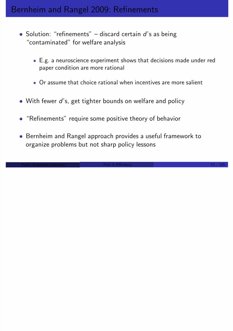
8/8/2019 Chetty - Public Economics Lectures
http://slidepdf.com/reader/full/chetty-public-economics-lectures 262/949
g g p y
“Re…nements” require some positive theory of behavior
Bernheim and Rangel approach provides a useful framework to
organize problems but not sharp policy lessons
Public Econom ics Lectures () Part 3: E¢ciency 93 / 105
Applied Welfare Analysis with Salience E¤ects
Chetty, Looney, and Kroft (2009) section 5
Derive partial-equilibrium formulas for incidence and e¢ciency costs
Focus here on e¢ciency cost analysis
Formulas do not rely on a speci…c positive theory, in the spirit of

8/8/2019 Chetty - Public Economics Lectures
http://slidepdf.com/reader/full/chetty-public-economics-lectures 263/949
y p p y pBernheim and Rangel (2009)
Public Econom ics Lectures () Part 3: E¢ciency 94 / 105
Welfare Analysis with Salience E¤ects: Setup
Two goods, x and y ; price of y is 1, pretax price of x is p .
Taxes: y untaxed. Unit sales tax on x at rate t S , which is notincluded in the posted price
Tax-inclusive price of x : q = p + t S

8/8/2019 Chetty - Public Economics Lectures
http://slidepdf.com/reader/full/chetty-public-economics-lectures 264/949
Public Econom ics Lectures () Part 3: E¢ciency 95 / 105
Welfare Analysis with Salience E¤ects: Setup
Representative consumer has wealth Z and utility u (x ) + v (y )
Letfx
(p , t S
,Z ), y
(p , t S
,Z )g denote bundle chosen by afully-optimizing agent
Let fx (p , t S ,Z ), y (p , t S ,Z )g denote empirically observed demands
Place no structure on these demand functions except for feasibility:

8/8/2019 Chetty - Public Economics Lectures
http://slidepdf.com/reader/full/chetty-public-economics-lectures 265/949
(p + t S )x (p , t S , Z ) + y (p , t S ,Z ) = Z
Public Econom ics Lectures () Part 3: E¢ciency 96 / 105
Welfare Analysis with Salience E¤ects: Setup
Price-taking …rms use y to produce x with cost fn. c
Firms optimize perfectly. Supply function S (p ) de…ned by:
p = c 0(S (p ))
Let εS = ∂S ∂p p S (p ) denote the price elasticity of supply
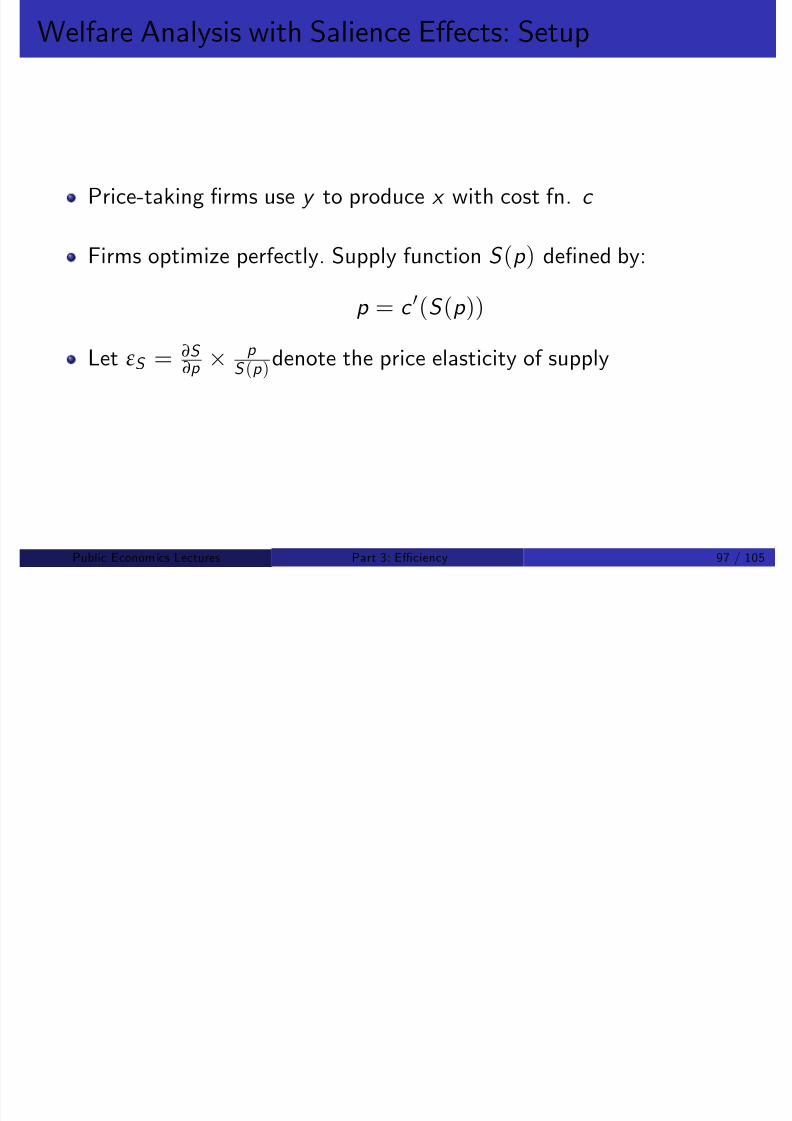
8/8/2019 Chetty - Public Economics Lectures
http://slidepdf.com/reader/full/chetty-public-economics-lectures 266/949
Public Econom ics Lectures () Part 3: E¢ciency 97 / 105
E¢ciency Cost with Salience E¤ects
De…ne excess burden using EV concept
Excess burden (EB) of introducing a revenue-generating sales tax t is:
EB (t S ) = Z e (p , 0,V (p , t S ,Z )) R (p , t S ,Z )

8/8/2019 Chetty - Public Economics Lectures
http://slidepdf.com/reader/full/chetty-public-economics-lectures 267/949
Public Econom ics Lectures () Part 3: E¢ciency 98 / 105
Preference Recovery Assumptions
A1 Taxes a¤ect utility only through their e¤ects on the chosenconsumption bundle. Agent’s indirect utility given taxes of (t E , t S ) is
V (p , t S , Z ) = u (x (p , t S ,Z )) + v (y (p , t S , Z ))
A2 When tax inclusive prices are fully salient, the agent chooses the sameallocation as a fully-optimizing agent:
x (p , 0,Z ) = x (p , 0,Z ) = arg maxx u (x ) + v (Z px )
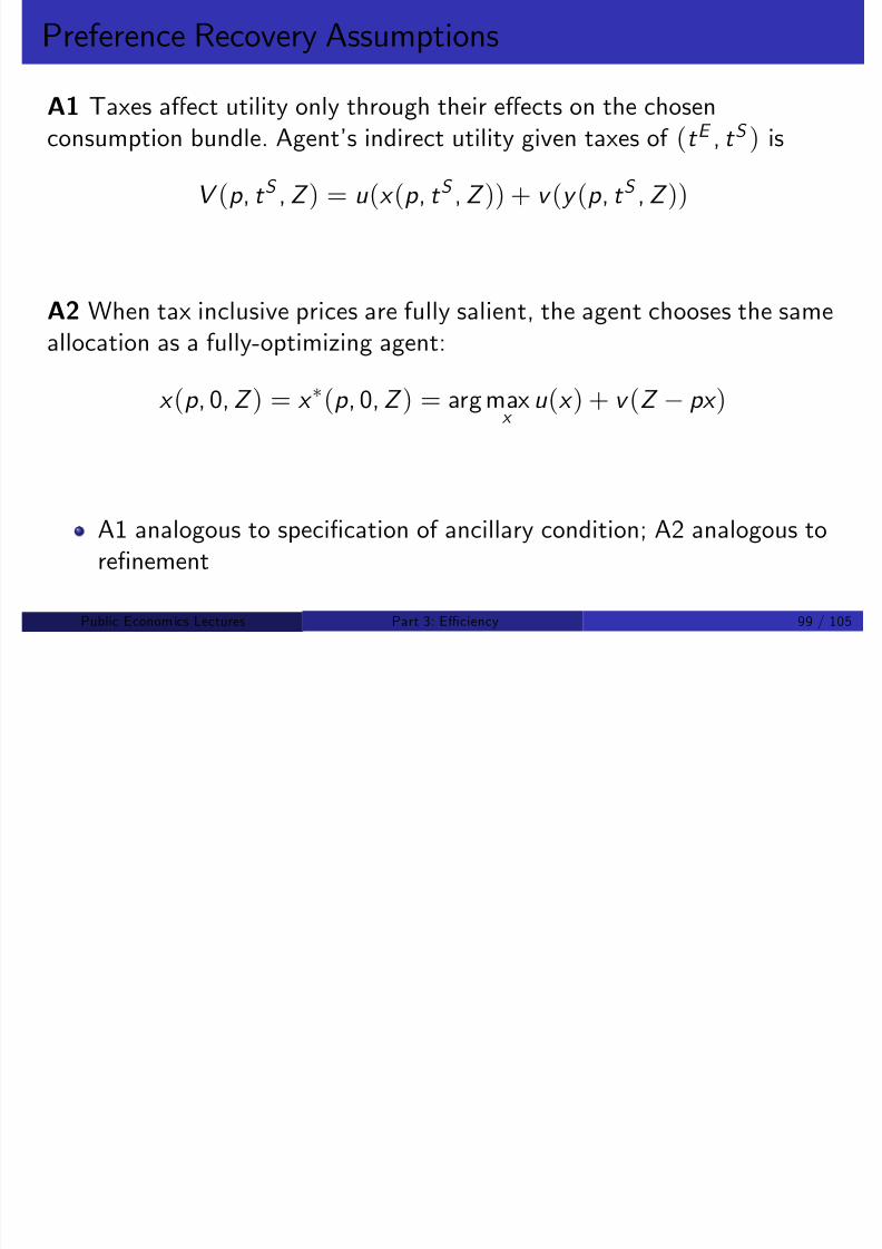
8/8/2019 Chetty - Public Economics Lectures
http://slidepdf.com/reader/full/chetty-public-economics-lectures 268/949
A1 analogous to speci…cation of ancillary condition; A2 analogous tore…nement
Public Econom ics Lectures () Part 3: E¢ciency 99 / 105
E¢ciency Cost with Salience E¤ects
Two steps in e¢ciency calculation:
1 Use price-demand x (p , 0, Z ) to recover utility as in standard model
2
Use tax-demand x (p , t S
,Z )to calculate V (p , t S
,Z ) and EB
8/8/2019 Chetty - Public Economics Lectures
http://slidepdf.com/reader/full/chetty-public-economics-lectures 269/949
Public Econom ics Lectures () Part 3: E¢ciency 100 / 105
Excess Burden with No Income E¤ect for Good x ( ∂x ∂Z = 0)
St p,
)(')0,( xu p x =
AB
C
D EG
H
F
I
0 + t S
xÝ p0, t SÞ
t S / x
/t S
t S/ x / /t S
/ x / / p
EB p ? 1
2Ýt SÞ 2 / x / /t S
/ x / / p/ x / /t S
p0

8/8/2019 Chetty - Public Economics Lectures
http://slidepdf.com/reader/full/chetty-public-economics-lectures 270/949
x0
x1 x
*
1 x
Source: Chetty, Looney, and Kroft (2009)
Public Econom ics Lectures () Part 3: E¢ciency 101 / 105
E¢ciency Cost: No Income E¤ects
In the case without income e¤ects ( ∂x ∂Z = 0), which implies utility is
quasilinear, excess burden of introducing a small tax t S is
EB (t S ) ' 1
2
(t S )2 ∂x /∂t S
∂x /∂p
∂x /∂t S
=1
2(θt S )2 εD
p + t S
Inattention reduces excess burden when dx /dZ = 0.
Intuition: tax tS induces behavioral response equivalent to a fully
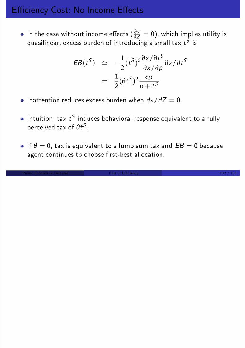
8/8/2019 Chetty - Public Economics Lectures
http://slidepdf.com/reader/full/chetty-public-economics-lectures 271/949
Intuition: tax t induces behavioral response equivalent to a fullyperceived tax of θt S .
If θ = 0, tax is equivalent to a lump sum tax and EB = 0 because
agent continues to choose …rst-best allocation.
Public Econom ics Lectures () Part 3: E¢ciency 102 / 105
E¢ciency Cost with Income E¤ects
Same formula, but all elasticities are now compensated:
EB (t S ) ' 1
2
(t S )2 ∂x c /∂t S
∂x c /
∂p ∂x c /∂t S
=1
2(θc t S )2 εc D
p + t S
Compensated price demand: dx c /dp = dx /dp + xdx /dZ
Compensated tax demand: dx c /dt S = dx /dt S + xdx /dZ

8/8/2019 Chetty - Public Economics Lectures
http://slidepdf.com/reader/full/chetty-public-economics-lectures 272/949
p
Compensated tax demand does not necessarily satisfy Slutskycondition dx c /dt S < 0 b/c it is not generated by utility maximization
Public Econom ics Lectures () Part 3: E¢ciency 103 / 105
E¢ciency Cost with Income E¤ects
EB (t S ) ' 1
2(t S )2 ∂x
c /∂t S
∂x c /∂p ∂x c /∂t S
=1
2
(θc t S )2 εc D
p + t S
With income e¤ects (dx /dZ > 0), making a tax less salient can raisedeadweight loss.
Tax can generate EB > 0 even if dx /dt S
= 0

8/8/2019 Chetty - Public Economics Lectures
http://slidepdf.com/reader/full/chetty-public-economics-lectures 273/949
Example: consumption of food and cars; agent who ignores tax oncars underconsumes food and has lower welfare.
Intuition: agent does not adjust consumption of x despite change innet-of-tax income, leading to a positive compensated elasticity.
Public Econom ics Lectures () Part 3: E¢ciency 104 / 105
Directions for Further Work on Behavioral Welfare Analysis
1 Normative analysis of tax policy
Consumption taxation: VAT vs. sales tax
Tax smoothing
Value of tax simpli…cation
2 Use similar approach to welfare analysis in other contexts

8/8/2019 Chetty - Public Economics Lectures
http://slidepdf.com/reader/full/chetty-public-economics-lectures 274/949
Design consumer protection laws and …nancial regulation in a lesspaternalistic manner by studying behavior in domains where incentivesare clear.
Public Econom ics Lectures () Part 3: E¢ciency 105 / 105
Public Economics LecturesPart 4: Optimal Taxation
Raj Chetty and Gregory A. Bruich
Harvard UniversityFall 2009
8/8/2019 Chetty - Public Economics Lectures
http://slidepdf.com/reader/full/chetty-public-economics-lectures 275/949
Fall 2009
Public Econom ics Lectures () Part 4: Optimal Taxation 1 / 121
Outline
1 Commodity Taxation I: Ramsey Rule
2 Commodity Taxation II: Production E¢ciency
3 Income Taxation I: Mirrlees Model
4 Income Taxation II: Atkinson-Stiglitz
5 Capital Income Taxation: Chamley-Judd result

8/8/2019 Chetty - Public Economics Lectures
http://slidepdf.com/reader/full/chetty-public-economics-lectures 276/949
p y
6 Optimal Transfer Programs
Public Econom ics Lectures () Part 4: Optimal Taxation 2 / 121
Optimal Commodity Taxation: Introduction
Now combine lessons on incidence and e¢ciency costs to analyzeoptimal design of commodity taxes
What is the best way to design taxes given equity and e¢ciencyconcerns?
Optimal commodity tax literature focuses on linear (t x
) tax system
( )

8/8/2019 Chetty - Public Economics Lectures
http://slidepdf.com/reader/full/chetty-public-economics-lectures 277/949
Non-linear (t (x )) tax systems considered in income tax literature
Public Econom ics Lectures () Part 4: Optimal Taxation 3 / 121
Second Welfare Theorem
Starting point: second-welfare theorem
Can achieve any Pareto-e¢cient allocation as a competitiveequilibrium with appropriate lump-sum transfers
Requires same assumptions as …rst welfare theorem plus one more:1 Complete markets (no externalities)2 Perfect information3 Perfect competition4 Lump-sum taxes/transfers across individuals feasible
If 1-4 hold, equity-e¢ciency trade-o¤ disappears and optimal taxbl i t i i l
8/8/2019 Chetty - Public Economics Lectures
http://slidepdf.com/reader/full/chetty-public-economics-lectures 278/949
problem is trivial
Simply implement lump sum taxes that meet distributional goals givenrevenue requirement
Problem: informationPublic Econom ics Lectures () Part 4: Optimal Taxation 4 / 121
Second Welfare Theorem: Information Constraints
To set the optimal lump-sum taxes, need to know the characteristics(ability) of each individual
But no way to make people reveal their ability at no cost
Incentive to misrepresent skill level
Tax instruments are therefore a fn. of economic outcomes
E.g. income, property, consumption of goods
! Distorts prices, a¤ecting behavior and generating DWB
Information constraints force us to move from the 1st best world of
8/8/2019 Chetty - Public Economics Lectures
http://slidepdf.com/reader/full/chetty-public-economics-lectures 279/949
Information constraints force us to move from the 1st best world of the second welfare theorem to the 2nd best world with ine¢cienttaxation
Cannot redistribute or raise revenue for public goods withoutgenerating e¢ciency costs
Public Econom ics Lectures () Part 4: Optimal Taxation 5 / 121
Four Central Results in Optimal Tax Theory
1 Ramsey (1927): inverse elasticity rule
2 Diamond and Mirrlees (1971): production e¢ciency
3 Atkinson and Stiglitz (1976): no consumption taxation with optimalnon-linear (including lump sum) income taxation
4 Chamley, Judd (1983): no capital taxation in in…nite horizon models

8/8/2019 Chetty - Public Economics Lectures
http://slidepdf.com/reader/full/chetty-public-economics-lectures 280/949
y ( ) p
Public Econom ics Lectures () Part 4: Optimal Taxation 6 / 121
Ramsey (1927) Tax Problem
Government sets taxes on uses of income in order to accomplish twoobjectives:
1 Raise total revenue of amount E
2 Minimize utility loss for agents in economy
Originally a problem set that Pigou assigned Ramsey

8/8/2019 Chetty - Public Economics Lectures
http://slidepdf.com/reader/full/chetty-public-economics-lectures 281/949
Public Econom ics Lectures () Part 4: Optimal Taxation 7 / 121
Ramsey Model: Key Assumptions
1 Lump sum taxation prohibited
2 Cannot tax all commodities (leisure untaxed)
3 Production prices …xed (and normalized to one):
p i = 1) q i = 1 + τ i

8/8/2019 Chetty - Public Economics Lectures
http://slidepdf.com/reader/full/chetty-public-economics-lectures 282/949
Public Econom ics Lectures () Part 4: Optimal Taxation 8 / 121
Ramsey Model: Setup
One individual (no redistributive concerns) with utility
u (x 1, .., x N , l )
subject to budget constraint
q 1x 1 + .. + q N x N wl + Z
Z = non wage income, w = wage rate

8/8/2019 Chetty - Public Economics Lectures
http://slidepdf.com/reader/full/chetty-public-economics-lectures 283/949
Consumption prices are q i
Public Econom ics Lectures () Part 4: Optimal Taxation 9 / 121
Ramsey Model: Consumer Behavior
Lagrangian for individual’s maximization problem:
L = u (x 1, .., x N , l ) + α(wl + Z (q 1x 1 + .. + q N x N ))
First order condition:u x i = αq i
Where α = ∂V /∂Z is marginal value of money for the individual
Yields demand functions x i (q , Z ) and indirect utility function V (q , Z )

8/8/2019 Chetty - Public Economics Lectures
http://slidepdf.com/reader/full/chetty-public-economics-lectures 284/949
( ) ( )where q = (w , q 1, .., q N )
Public Econom ics Lectures () Part 4: Optimal Taxation 10 / 121
Ramsey Model: Government’s Problem
Government solves either the maximization problem
max V (q , Z )
subject to the revenue requirement
τ x =N
∑ i =1
τ i x i (q , Z ) E
Or, equivalently, minimize excess burden of the tax system

8/8/2019 Chetty - Public Economics Lectures
http://slidepdf.com/reader/full/chetty-public-economics-lectures 285/949
min EB (q ) = e (q , V (q , Z )) e (p , V (q , Z )) E
subject to the same revenue requirement
Public Econom ics Lectures () Part 4: Optimal Taxation 11 / 121
Ramsey Model: Government’s Problem
For maximization problem, Lagrangian for government is:
LG = V (q , Z ) + λ[∑ i
τ i x i (q , Z ) E ]
)∂LG
∂q i =∂V
∂q i |{z} Priv. Welfare
Loss to Indiv.
+ λ[ x i |{z} Mechanical
E¤ect
+∑ j τ j ∂x j /∂q i | { z }
Behavioral
Response
] = 0
Using Roy’s identity ( ∂V ∂q i
= αx i ):

8/8/2019 Chetty - Public Economics Lectures
http://slidepdf.com/reader/full/chetty-public-economics-lectures 286/949
(λ α)x i + λ∑ j
τ j ∂x j /∂q i = 0
Note connection to marginal excess burden formula, where λ = 1 andα = 1
Public Econom ics Lectures () Part 4: Optimal Taxation 12 / 121
Ramsey Optimal Tax Formula
Optimal tax rates satisfy system of N equations and N unknowns:
∑ j
τ j ∂x j
∂q i =
x i
λ(λ α)
Same formula can be derived using a perturbation argument, which is
more intuitive

8/8/2019 Chetty - Public Economics Lectures
http://slidepdf.com/reader/full/chetty-public-economics-lectures 287/949
Public Econom ics Lectures () Part 4: Optimal Taxation 13 / 121
Ramsey Formula: Perturbation Argument
Suppose government increases τ i by d τ i
E¤ect of tax increase on social welfare is sum of e¤ect on governmentrevenue and private surplus
Marginal e¤ect on government revenue:dR = x i d τ i +∑
j
τ j dx j
Marginal e¤ect on private surplus:
dU =∂V
∂q i d τ i

8/8/2019 Chetty - Public Economics Lectures
http://slidepdf.com/reader/full/chetty-public-economics-lectures 288/949
q
= αx i d τ i
Optimum characterized by balancing the two marginal e¤ects:
dU + λdR = 0
Public Econom ics Lectures () Part 4: Optimal Taxation 14 / 121

8/8/2019 Chetty - Public Economics Lectures
http://slidepdf.com/reader/full/chetty-public-economics-lectures 289/949
Ramsey Formula: Compensated Elasticity Representation
θ is independent of i and measures the value for the government of introducing a $1 lump sum tax
θ = λ α λ∂(
∑ j
τ j x j )/∂Z
Three e¤ects of introducing a $1 lumpsum tax:
1 Direct value for the government is λ2 Loss in welfare for the individual is α3 Behavioral e¤ect ! loss in tax revenue of ∂(∑ j τ j x j )/∂Z

8/8/2019 Chetty - Public Economics Lectures
http://slidepdf.com/reader/full/chetty-public-economics-lectures 290/949
Can demonstrate that θ > 0 ) λ > α at the optimum using Slutskymatrix
Public Econom ics Lectures () Part 4: Optimal Taxation 16 / 121
Intuition for Ramsey Formula: Index of Discouragement
1x i ∑ j
τ j ∂hi
∂q j =
θλ
Suppose revenue requirement E is small so that all taxes are also small
Then tax τ j on good j reduces consumption of good i (holding utilityconstant) by approximately
dhi = τ j ∂hi
∂q j
Numerator of LHS: total reduction in consumption of good i
Dividing by x yields % reduction in consumption of each good i
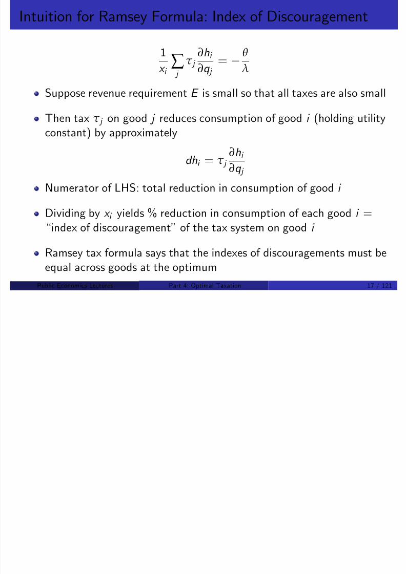
8/8/2019 Chetty - Public Economics Lectures
http://slidepdf.com/reader/full/chetty-public-economics-lectures 291/949
Dividing by x i yields % reduction in consumption of each good i =“index of discouragement” of the tax system on good i
Ramsey tax formula says that the indexes of discouragements must beequal across goods at the optimum
Public Econom ics Lectures () Part 4: Optimal Taxation 17 / 121
Special Case 1: Inverse Elasticity Rule
Introducing elasticities, we can write formula as:
N
∑ j =1
τ j 1 + τ j
εc ij =
θ
λ
Consider special case where εij = 0 if i 6= j
Slutsky matrix is diagonal
Obtain classic inverse elasticity rule:

8/8/2019 Chetty - Public Economics Lectures
http://slidepdf.com/reader/full/chetty-public-economics-lectures 292/949
τ i 1 + τ i
=θ
λ
1
εii
Public Econom ics Lectures () Part 4: Optimal Taxation 18 / 121
Special Case 2: Uniform Taxation
Suppose εij = 0 if i 6= j and εx i ,w =∂h
i w w hi constant
Using following identity, ∑ j
∂hi
∂q j q j + ∂hi
∂w w = 0, we obtain
∂hi
∂q i q i = ∂hi
∂w w
Proof of identity (J good economy, no labor):
∑ j
∂hi
∂q j q j = ∑ j 6=i
∂h j
∂q i q j +∂hi
∂q i q i
∂hj qj ∂hi qi

8/8/2019 Chetty - Public Economics Lectures
http://slidepdf.com/reader/full/chetty-public-economics-lectures 293/949
= ∑ j 6=i
∂h j q j
∂q i +
∂hi q i
∂q i hi
=∂e
∂q i hi = 0
Public Econom ics Lectures () Part 4: Optimal Taxation 19 / 121
Special Case 2: Uniform Taxation
Then immediately obtain1
x i τ i =
θ
λ
1∂hi
∂q i
=θ
λ
1∂hi
∂w w
τ i
q i
=θ
λ
1∂hi
∂w w x i
=θ
λ
εx i ,w
With constant εx i ,w ,τ i q i
is constant ! uniform taxation
Corlett and Hague (1953): 3 good model, uniform tax optimal if allgoods are equally complementary with labor (and labor is untaxed)
More generally, lower taxes for goods complementary to labor

8/8/2019 Chetty - Public Economics Lectures
http://slidepdf.com/reader/full/chetty-public-economics-lectures 294/949
Di¤erent intuition than Goulder and Williams (2003) argument forwhy taxing goods complementary with labor is undesirable
Here, higher substitutability with labor ) higher own price elasticity;no pre-existing tax on labor
Public Econom ics Lectures () Part 4: Optimal Taxation 20 / 121
Ramsey Formula: Limitations
Ramsey solution: tax inelastic goods to minimize e¢ciency costs
But does not take into account redistributive motives
Presumably necessities are more inelastic than luxuries
Therefore, optimal Ramsey tax system is likely to be regressive
Diamond (1975) extends Ramsey model to take redistributive motivesi t t

8/8/2019 Chetty - Public Economics Lectures
http://slidepdf.com/reader/full/chetty-public-economics-lectures 295/949
into account
Public Econom ics Lectures () Part 4: Optimal Taxation 21 / 121
Diamond 1975: Many-Person Model
H individuals with utilities u 1, .., u h, .., u H
Aggregate consumption of good i is
X i (q ) = ∑ h
x hi
Govt. chooses tax rates τ i and a lump sum transfer T 0 tomaximize social welfare:
max W (V 1, .., V H ) s.t.N
∑ i 1
τ i X i E + T

8/8/2019 Chetty - Public Economics Lectures
http://slidepdf.com/reader/full/chetty-public-economics-lectures 296/949
i =1
Consider e¤ect of increasing tax on good i by d τ i
Public Econom ics Lectures () Part 4: Optimal Taxation 22 / 121
Diamond: E¤ect of Tax Increase
E¤ect of perturbation on revenue:
dE = X i d τ i +∑ j
τ j dX j = d τ i [X i +∑ j
τ j ∂X j
∂q i ]
E¤ect on individual h’s welfare:
dU h =∂V h
∂q i d τ i = αhx hi d τ i
E¤ect on total private welfare:
dW = ∑ h
(∂W /∂V h )αhx hi d τ i = d τ i [∑ h
βh x hi ]
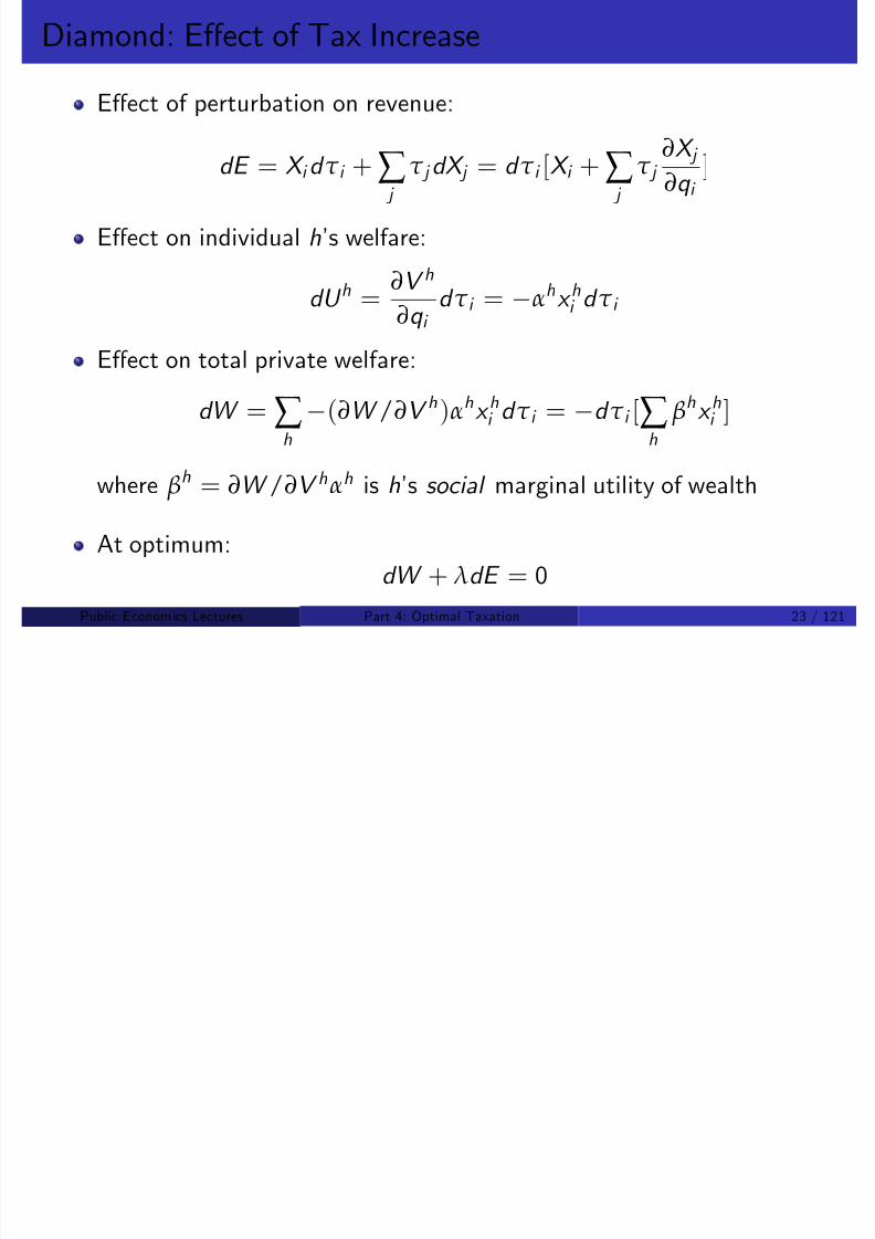
8/8/2019 Chetty - Public Economics Lectures
http://slidepdf.com/reader/full/chetty-public-economics-lectures 297/949
where βh = ∂W /∂V hαh is h’s social marginal utility of wealth
At optimum:dW + λdE = 0
Public Econom ics Lectures () Part 4: Optimal Taxation 23 / 121
Diamond: Many-Person Optimal Tax Formula
Solving yields formula for optimal tax rates:
∑ j
τ j ∂X j
∂q i =
X i
λ[λ
∑ h βhx hi X i
]
With no redistributive tastes (Ramsey case): βh = α constant
Obtain same formula as before (in terms of uncompensated elasticities)
With redistributive tastes, βh lower for higher income individualsh h

8/8/2019 Chetty - Public Economics Lectures
http://slidepdf.com/reader/full/chetty-public-economics-lectures 298/949
New term∑ h βh x hi
X i is average social marginal utility, weighted by
consumption of good i
Public Econom ics Lectures () Part 4: Optimal Taxation 24 / 121
Diamond Formula: Special Case
When uncompensated cross price elasticities are zero, optimal taxrates satisfy
τ i 1 + τ
i
=1
u
ii 1∑ h βhx hi λX
i !τ i still inversely proportional to the elasticity but term in brackets nolonger constant across goods
For goods that are consumed by the poor (∑ h
βhx h
i
)/(λX i ) is large
Optimal tax rate for these goods is lower (elasticities being the same)
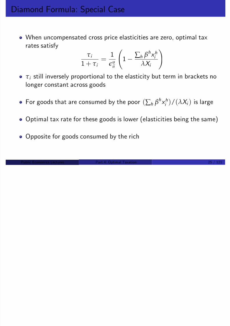
8/8/2019 Chetty - Public Economics Lectures
http://slidepdf.com/reader/full/chetty-public-economics-lectures 299/949
Opposite for goods consumed by the rich
Public Econom ics Lectures () Part 4: Optimal Taxation 25 / 121
Diamond: Optimal Transfer
In this model, optimal for the government to pay a uniform transferT on top of tax rates
With redistributive tastes, T > 0
With no redistributive tastes, ideally set T = E
This is ruled out by constraint T 0
Constraint arises because poor cannot a¤ord to pay lump sum tax
8/8/2019 Chetty - Public Economics Lectures
http://slidepdf.com/reader/full/chetty-public-economics-lectures 300/949
Constraint arises because poor cannot a¤ord to pay lump sum tax
Public Econom ics Lectures () Part 4: Optimal Taxation 26 / 121
Diamond and Mirrlees (1971)
Previous analysis assumed …xed producer prices
Diamond and Mirrlees (1971) relax this assumption by modelling
production
Two major results
1 Production e¢ciency: even in an economy where …rst-best isunattainable, optimal policy maintains production e¢ciency
2 Characterize optimal tax rates with endogenous prices and show that

8/8/2019 Chetty - Public Economics Lectures
http://slidepdf.com/reader/full/chetty-public-economics-lectures 301/949
Characterize optimal tax rates with endogenous prices and show thatRamsey rule can be applied
Public Econom ics Lectures () Part 4: Optimal Taxation 27 / 121
Lipsey and Lancaster (1956): Theory of the Second Best
Standard optimal policy results only hold with single deviation from…rst best
Ex: Ramsey formulas invalid if there are pre-existing distortions,imperfect competition, etc.
In second-best, anything is possible
Policy changes that would increase welfare in a model with a single
deviation from …rst best need not do so in second-best
Ex: tari¤s can improve welfare by reducing distortions in other part of
8/8/2019 Chetty - Public Economics Lectures
http://slidepdf.com/reader/full/chetty-public-economics-lectures 302/949
economy
Destructive result for welfare economics
Public Econom ics Lectures () Part 4: Optimal Taxation 28 / 121
Diamond and Mirrlees: Production E¢ciency
Diamond and Mirrlees result was an advance because it showed ageneral policy lesson even in second-best environment
Example: Suppose government can tax consumption goods and alsoproduces some goods on its own (e.g. postal services)
May have intuition that government should try to generate pro…ts inpostal services by increasing the price of stamps
This intuition is wrong: optimal to have no distortions in production
of goods
Bottom line: only tax goods that appear directly in agent’s utilityf
8/8/2019 Chetty - Public Economics Lectures
http://slidepdf.com/reader/full/chetty-public-economics-lectures 303/949
functions
Should not distort production decisions via taxes on intermediategoods, tari¤s, etc.
Public Econom ics Lectures () Part 4: Optimal Taxation 29 / 121
Diamond and Mirrlees Model
Two good (labor, consumption), one consumer model
Begin with this case because results easily seen graphically
In one consumer case, restrict attention to situation where cannotimpose lump sum tax
Corresponding case in many consumer case: permit only uniformlump sum taxation

8/8/2019 Chetty - Public Economics Lectures
http://slidepdf.com/reader/full/chetty-public-economics-lectures 304/949
Public Econom ics Lectures () Part 4: Optimal Taxation 30 / 121
Diamond and Mirrlees Model: Setup
Government directly chooses allocations and production subject torequirement that allocation must be supported by an equilibrium pricevector
Government levies tax τ on consumption to fund revenue requirementE
Individual budget constraint: (1 + τ )c l
First trace out demand as a function of tax rates: the o¤er curve

8/8/2019 Chetty - Public Economics Lectures
http://slidepdf.com/reader/full/chetty-public-economics-lectures 305/949
Public Econom ics Lectures () Part 4: Optimal Taxation 31 / 121
Consumer’s O¤er Curve

8/8/2019 Chetty - Public Economics Lectures
http://slidepdf.com/reader/full/chetty-public-economics-lectures 306/949
Public Econom ics Lectures () Part 4: Optimal Taxation 32 / 121
Diamond and Mirrlees: Social Planner’s problem
Government’s problem is to
maxτ
V (q ) = u (x (q ), l (q ))
subject to two constraints
1 Revenue constraint: τ c E
2
Production constraint: x = f (l )
Replace these constraints by (l , c ) 2 H where H is feasible production
8/8/2019 Chetty - Public Economics Lectures
http://slidepdf.com/reader/full/chetty-public-economics-lectures 307/949
set taking into account the tax revenue needed
Public Econom ics Lectures () Part 4: Optimal Taxation 33 / 121
Production Set with Revenue Requirement

8/8/2019 Chetty - Public Economics Lectures
http://slidepdf.com/reader/full/chetty-public-economics-lectures 308/949
Public Econom ics Lectures () Part 4: Optimal Taxation 34 / 121
First Best: Optimal Lump Sum Tax

8/8/2019 Chetty - Public Economics Lectures
http://slidepdf.com/reader/full/chetty-public-economics-lectures 309/949
Public Econom ics Lectures () Part 4: Optimal Taxation 35 / 121
Second Best: Optimal Distortionary Tax
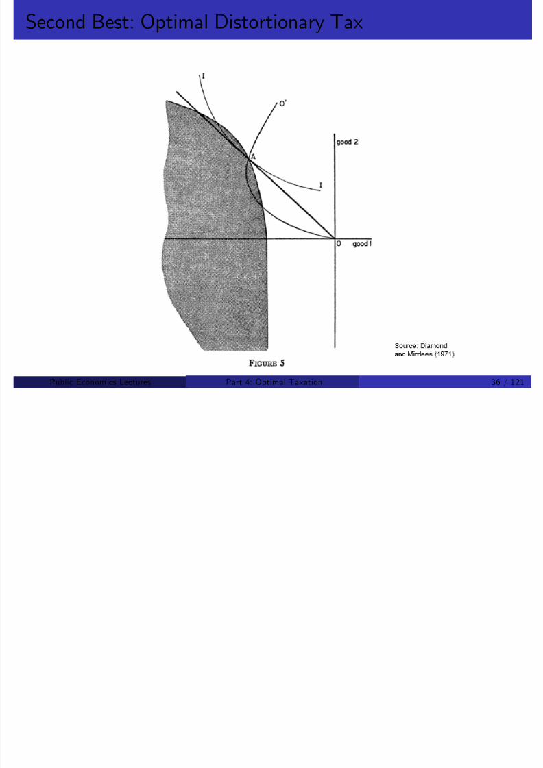
8/8/2019 Chetty - Public Economics Lectures
http://slidepdf.com/reader/full/chetty-public-economics-lectures 310/949
Public Econom ics Lectures () Part 4: Optimal Taxation 36 / 121
Production E¢ciency Result in One-Consumer Model
Key insight: allocation with optimal distortionary tax is still on PPF
Equilibrium price vector q places consumer on PPF, subject torevenue requirement
With lump sum tax, tangency between PPF and consumer’s
indi¤erence curve, yielding higher welfare

8/8/2019 Chetty - Public Economics Lectures
http://slidepdf.com/reader/full/chetty-public-economics-lectures 311/949
Public Econom ics Lectures () Part 4: Optimal Taxation 37 / 121
Diamond and Mirrlees: General Model
Many consumers, many goods and inputs
Important assumption: either constant returns to scale in production(no pro…ts) or pure pro…ts can be fully taxed
With this assumption, pro…ts do not enter social welfare fn

8/8/2019 Chetty - Public Economics Lectures
http://slidepdf.com/reader/full/chetty-public-economics-lectures 312/949
Public Econom ics Lectures () Part 4: Optimal Taxation 38 / 121
Diamond and Mirrlees: General Model
Government chooses the vector q = p + τ to
max W (V 1(q ), .., V H (q )) s.t.∑ i
τ i X i (q ) E
where X i (q ) = ∑ h x h
i
(q ), sum of individual demands given after-taxprices q
Constraint can be replaced by
X (q ) = ∑ h x
h
(q ) 2 H
where H is the production set which takes into account thei E f h

8/8/2019 Chetty - Public Economics Lectures
http://slidepdf.com/reader/full/chetty-public-economics-lectures 313/949
government requirement E of the government
E¢ciency result: at the optimum q , X (q ) is on the boundary of H
Public Econom ics Lectures () Part 4: Optimal Taxation 39 / 121
Proof of Production E¢ciency Result
Suppose X (q ) is in the interior of H
Then take a commodity i that is desired by everybody, and decreasetax on i by d τ i
Then X (q d τ i ) 2 H for d τ i small by continuity of demandfunctions; so it is a feasible point
Everybody is better because of that change:
dV h = V hq i d τ i = V hR x hi d τ i
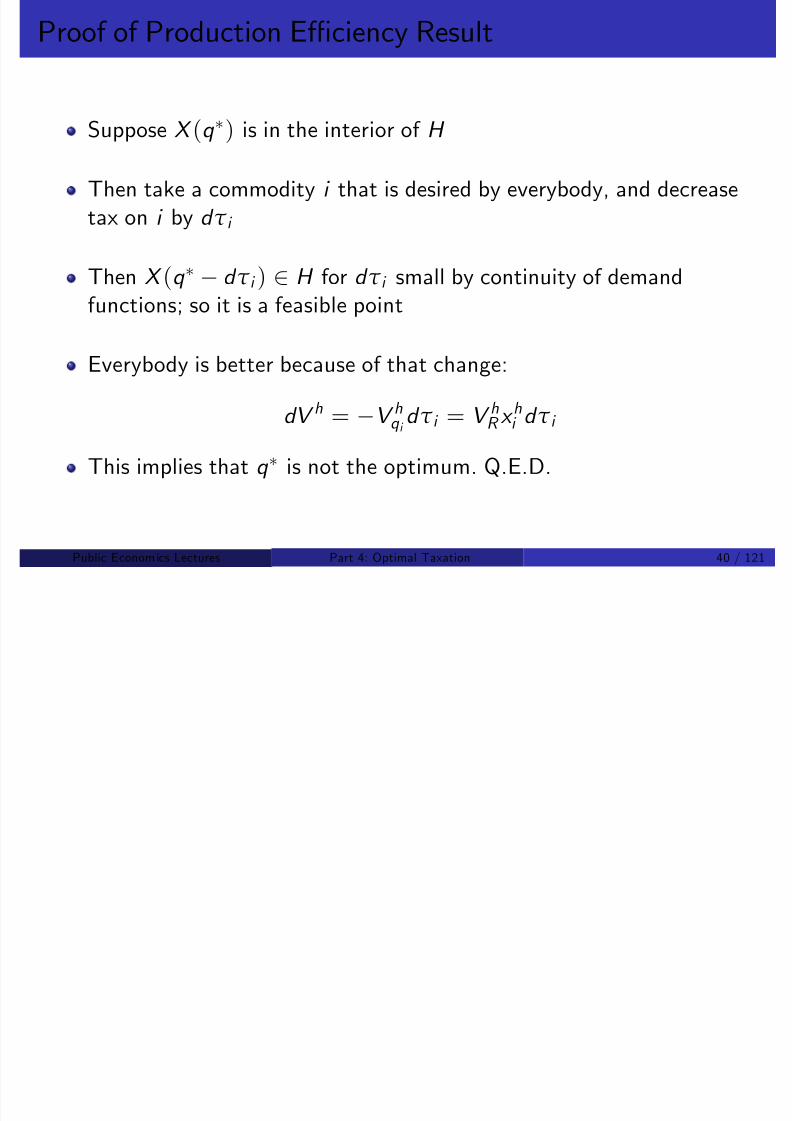
8/8/2019 Chetty - Public Economics Lectures
http://slidepdf.com/reader/full/chetty-public-economics-lectures 314/949
This implies that q is not the optimum. Q.E.D.
Public Econom ics Lectures () Part 4: Optimal Taxation 40 / 121
Production E¢ciency Result
Result can be stated algebraically using MRS and MRT
Consider two industries, x and y and two inputs, K and L
Then with the optimal tax schedule, production is e¢cient:
MRTS x KL = MRTS
y KL
This is true even though allocation is ine¢cient:
MRT xy 6= MRS xy

8/8/2019 Chetty - Public Economics Lectures
http://slidepdf.com/reader/full/chetty-public-economics-lectures 315/949
Public Econom ics Lectures () Part 4: Optimal Taxation 41 / 121
Policy Consequences: Public Sector Production
Public sector production should be e¢cient
If there is a public sector producing some goods, it should:
Face the same prices as the private sector
Choose production with the unique goal of maximizing pro…ts, notgenerating government revenue
Ex. postal services, electricity, health care, ...

8/8/2019 Chetty - Public Economics Lectures
http://slidepdf.com/reader/full/chetty-public-economics-lectures 316/949
Public Econom ics Lectures () Part 4: Optimal Taxation 42 / 121
Policy Consequences: No Taxation of Intermediate Goods
Intermediate goods: goods that are neither direct inputs or outputsto indiv. consumption
Taxes on transactions between …rms would distort production
8/8/2019 Chetty - Public Economics Lectures
http://slidepdf.com/reader/full/chetty-public-economics-lectures 317/949
Public Econom ics Lectures () Part 4: Optimal Taxation 43 / 121
Policy Consequences: No Taxation of Intermediate Goods
Consider two industries, with labor as the primary input
Intermediate good A, …nal good B
Industry A:
Uses labor l A
to produce good A
One for one technology
Industry B :
Uses good A and labor l B to produce good B x B = F (l B , x A )
Constant returns to scale
With wage rate w , the producer price of good A is p A = w

8/8/2019 Chetty - Public Economics Lectures
http://slidepdf.com/reader/full/chetty-public-economics-lectures 318/949
Suppose that good A is taxed at rate τ
Then the cost for …rm B of good A is w + τ
Public Econom ics Lectures () Part 4: Optimal Taxation 44 / 121
Policy Consequences: No Taxation of Intermediate Goods
Firm B chooses l and x A to max
F (l B , x A) wl (w + τ )x A
) F l = w and F x A = w + τ > F l
Aggregate production is ine¢cient:
Decrease l B and increase l A a small amount
Then x A increases
Total production of good B increases
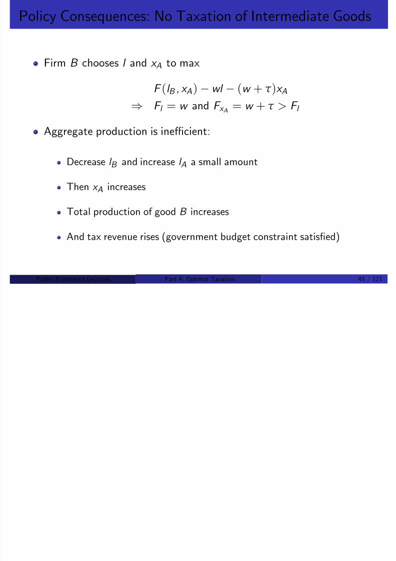
8/8/2019 Chetty - Public Economics Lectures
http://slidepdf.com/reader/full/chetty-public-economics-lectures 319/949
And tax revenue rises (government budget constraint satis…ed)
Public Econom ics Lectures () Part 4: Optimal Taxation 45 / 121
Policy Consequences: No Taxation of Intermediate Goods
Computers:
Sales to …rms should be untaxedBut sales to consumers should be taxed
In practice, tax policy often follows precisely the opposite rule
Ex. Diesel fuel tax studied by Marion and Muehlegger (2008)

8/8/2019 Chetty - Public Economics Lectures
http://slidepdf.com/reader/full/chetty-public-economics-lectures 320/949
Public Econom ics Lectures () Part 4: Optimal Taxation 46 / 121
Policy Consequences: Tari¤s
In open economy, the production set is extended because it is possibleto trade at linear prices (for a small country) with other countries
Diamond-Mirrlees result: small open economy should be on thefrontier of the extended production set
Implies that no tari¤s should be imposed on goods and inputsimported or exported by the production sector
Ex. sales of IBM computers to other countries should be untaxed
Ex. purchases of oil by oil companies should be untaxed
8/8/2019 Chetty - Public Economics Lectures
http://slidepdf.com/reader/full/chetty-public-economics-lectures 321/949
Ex. should be no special tari¤ on imported cars from Japan, but
should bear same commodity tax as cars made in US
Public Econom ics Lectures () Part 4: Optimal Taxation 47 / 121
Diamond and Mirrlees: Optimal Tax Rates
Optimal tax formulas take the same form as the solution to Ramseymany-persons problem
Result holds even where producer prices are not constant
Same formulas as in Ramsey just by replacing the p ’s by the actualp ’s that arise in equilibrium
Key point: Incidence in the production sector and GE responses canbe completely ignored in formulas

8/8/2019 Chetty - Public Economics Lectures
http://slidepdf.com/reader/full/chetty-public-economics-lectures 322/949
Public Econom ics Lectures () Part 4: Optimal Taxation 48 / 121
Diamond and Mirrlees Model: Key Assumptions
Result hinges on key assumptions about govt’s ability to:
1 Set a full set of di¤erentiated tax rates on each input and output
2 Tax away fully pure pro…ts (or production is constant-returns-to-scale)
A2 rules out improving welfare by taxing pro…table industries toimprove distribution at expense of prod. e¤.
These assumptions e¤ectively separate the production andconsumption problems

8/8/2019 Chetty - Public Economics Lectures
http://slidepdf.com/reader/full/chetty-public-economics-lectures 323/949
Public Econom ics Lectures () Part 4: Optimal Taxation 49 / 121
Diamond and Mirrlees Result: Limitations
Practical relevance of the result is a bit less clear
Ex. Assumption 1 is not realistic (Naito 1999)
Skilled and unskilled labor inputs ought to be di¤erentiated
Not the case in current income tax system
In such cases, may be optimal to:
1 Subsidize low skilled intensive industries
2 Set tari¤s on low skilled intensive imported goods (to protect domestic

8/8/2019 Chetty - Public Economics Lectures
http://slidepdf.com/reader/full/chetty-public-economics-lectures 324/949
2 Set tari¤s on low skilled intensive imported goods (to protect domesticindustry)
Public Econom ics Lectures () Part 4: Optimal Taxation 50 / 121
Optimal Income Taxation: Outline
1 Optimal Static Income Taxation: Mirrlees (1971)
2 Empirical Implementation of Mirrlees Model: Saez (2001)
3 Income and Commodity Taxation: Atkinson and Stiglitz (1976)
4 Optimal Transfer Programs: Saez (2002)
8/8/2019 Chetty - Public Economics Lectures
http://slidepdf.com/reader/full/chetty-public-economics-lectures 325/949
Public Econom ics Lectures () Part 4: Optimal Taxation 51 / 121
Key Concepts for Taxes/Transfers
Let T (z ) denote tax liability as a function of earnings z
1 Transfer bene…t with zero earnings T (0) [sometimes calleddemogrant or lumpsum grant]
2 Marginal tax rate T 0(z ): individual keeps 1 T 0(z ) for an additional$1 of earnings (relevant for intensive margin labor supply responses)
3 Participation tax rate τ p = [T (z ) T (0)]/z : individual keepsfraction 1 τ p of earnings when moving from zero earnings to
earnings z :
z T (z ) = T (0) + z [T (z ) T (0)] = T (0) + z (1 τ p )
Relevant for extensive margin labor supply responses

8/8/2019 Chetty - Public Economics Lectures
http://slidepdf.com/reader/full/chetty-public-economics-lectures 326/949
Relevant for extensive margin labor supply responses
4 Break-even earnings point z : point at which T (z ) = 0
Public Econom ics Lectures () Part 4: Optimal Taxation 52 / 121
US Tax/Transfer System, single parent with 2 children, 2009
$0
$10,000
$20,000
$30,000
$40,000
$50,000
$ 0
$ 5 , 3
8 3
$ 1 0 , 7
6 5
$ 1 6 , 1
4 8
$ 2 1 , 5
3 0
$ 2 6 , 9
1 3
$ 3 2 , 2
9 5
$ 3 7 , 6
7 8
$ 4 3 , 0
6 0
$ 4 8 , 4
4 3
Gross Earnings (with employer payroll taxes)
D i s p o s a b l e E
a r n i n g s
$0
$10,000
$20,000
$30,000
$40,000
$50,000
Welfare:TANF+SNAP
Tax credits:EITC+CTC
Earnings aftertaxes
45 Degree Line

8/8/2019 Chetty - Public Economics Lectures
http://slidepdf.com/reader/full/chetty-public-economics-lectures 327/949
Source: Saez 2010 AEA Clark Lecture
Public Econom ics Lectures () Part 4: Optimal Taxation 53 / 121
Optimal Income Tax with No Behavioral Responses
Utility u (c ) strictly increasing and concave
Same for everybody where c is after tax income
Income is z and is …xed for each individual, c = z T (z ) whereT (z ) is tax on z
Government maximizes Utilitarian objective:
Z ∞0
u (z T (z ))h(z )dz
Subject to budget constraint T (z )h(z )dz E (multiplier λ)

8/8/2019 Chetty - Public Economics Lectures
http://slidepdf.com/reader/full/chetty-public-economics-lectures 328/949
j g
R ( ) ( ) ( p )
Public Econom ics Lectures () Part 4: Optimal Taxation 54 / 121
Optimal Income Tax without Behavioral Responses
Lagrangian for this problem is:
L = [u (z T (z )) + λT (z )]h(z )
First order condition:
T (z ) : 0 = ∂L/∂T (z ) = [u 0(z T (z )) + λ]h(z )) u 0(z T (z )) = λ
) z T (z ) = c constant for all z
) c = z E
where z =R
zh(z )dz average income
100% marginal tax rate; perfect equalization of after-tax income

8/8/2019 Chetty - Public Economics Lectures
http://slidepdf.com/reader/full/chetty-public-economics-lectures 329/949
g p q
Utilitarianism with diminishing marginal utility leads to egalitarianism
Public Econom ics Lectures () Part 4: Optimal Taxation 55 / 121
Mirrlees 1971: Incorporating Behavioral Responses
Standard labor supply model: Individual maximizes
u (c , l ) s.t. c = wl T (wl )
where c is consumption, l labor supply, w wage rate, T (.) income tax
Individuals di¤er in ability w distributed with density f (w )
Govt social welfare maximization: Govt maximizes
SWF = Z G (u (c , l ))f (w )dw )
s.t. resource constraint
Z T (wl )f (w )dw E
and individual FOC w (1 T 0)uc + ul = 0
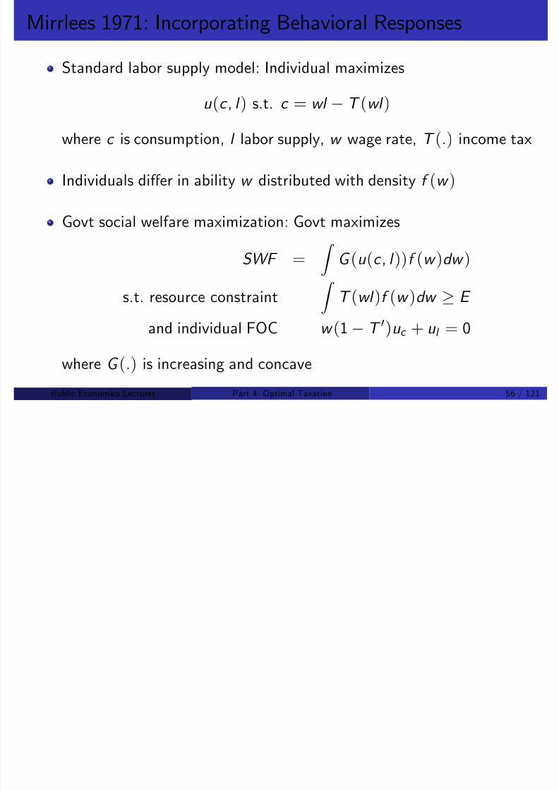
8/8/2019 Chetty - Public Economics Lectures
http://slidepdf.com/reader/full/chetty-public-economics-lectures 330/949
and individual FOC w (1 T )u c + u l 0
where G (.) is increasing and concave
Public Econom ics Lectures () Part 4: Optimal Taxation 56 / 121
Mirrlees 1971: Results
Optimal income tax trades-o¤ redistribution and e¢ciency
T (.) < 0 at bottom (transfer)
T (.) > 0 further up (tax) [full integration of taxes/transfers]
Mirrlees formulas are a complex fn. of primitives, with only a fewgeneral results
1 0 T 0(.) 1, T 0(.) 0 is non-trivial and rules out EITC [Seade1976]
2 Marginal tax rate T 0(.) should be zero at the top if skill distribution

8/8/2019 Chetty - Public Economics Lectures
http://slidepdf.com/reader/full/chetty-public-economics-lectures 331/949
bounded [Sadka-Seade]
Public Econom ics Lectures () Part 4: Optimal Taxation 57 / 121
Mirrlees: Subsequent Work
Mirrlees model had a profound impact on information economics
Ex. models with asymmetric information in contract theory
But until late 1990s, Mhad little impact on practical tax policy
Recently, Mirrlees model connected to empirical literature
Diamond (1998), Piketty (1997), and Saez (2001)
Su¢cient statistic formulas in terms of labor supply elasticities insteadof primitives

8/8/2019 Chetty - Public Economics Lectures
http://slidepdf.com/reader/full/chetty-public-economics-lectures 332/949
Public Econom ics Lectures () Part 4: Optimal Taxation 58 / 121
Optimal Income Taxation: Su¢cient Statistic Formulas
1 Revenue-maximizing linear tax (La¤er curve)
2 Top income tax rate (Saez 2001)
3 Full income tax schedule (Saez 2001)
See also section 4 of Chetty (Ann. Rev. 2009)

8/8/2019 Chetty - Public Economics Lectures
http://slidepdf.com/reader/full/chetty-public-economics-lectures 333/949
Public Econom ics Lectures () Part 4: Optimal Taxation 59 / 121
Revenue-Maximizing Tax Rate: La¤er Curve
With a constant tax rate τ , reported income z depends on 1 τ (net-of-tax rate)
Tax Revenue R (τ ) = τ z (1 τ ) is inverse-U shaped:
R (τ = 0) = 0 (no taxes) and R (τ = 1) = 0 (nobody works)
Tax rate τ that maximizes R :
0 =R 0
(τ
) =z
τ
dz /d (1
τ )) τ MAX = 1/(1 + ε)
where ε = [(1 τ )/Z ]dz /d (1 τ ) is the taxable income elasticity

8/8/2019 Chetty - Public Economics Lectures
http://slidepdf.com/reader/full/chetty-public-economics-lectures 334/949
Strictly ine¢cient to have τ > τ
Public Econom ics Lectures () Part 4: Optimal Taxation 60 / 121
Optimal Top Income Tax Rate
Now consider constant mtr τ above …xed income threshold z
Derive optimal τ using perturbation argument
Assume away income e¤ects εc = εu = ε
Diamond (1996) shows this is a key theoretical simpli…cation
Assume that there are N individuals above z
Denote by z m (1 τ ) their average income, which depends onnet-of-tax rate 1 τ
8/8/2019 Chetty - Public Economics Lectures
http://slidepdf.com/reader/full/chetty-public-economics-lectures 335/949
Public Econom ics Lectures () Part 4: Optimal Taxation 61 / 121
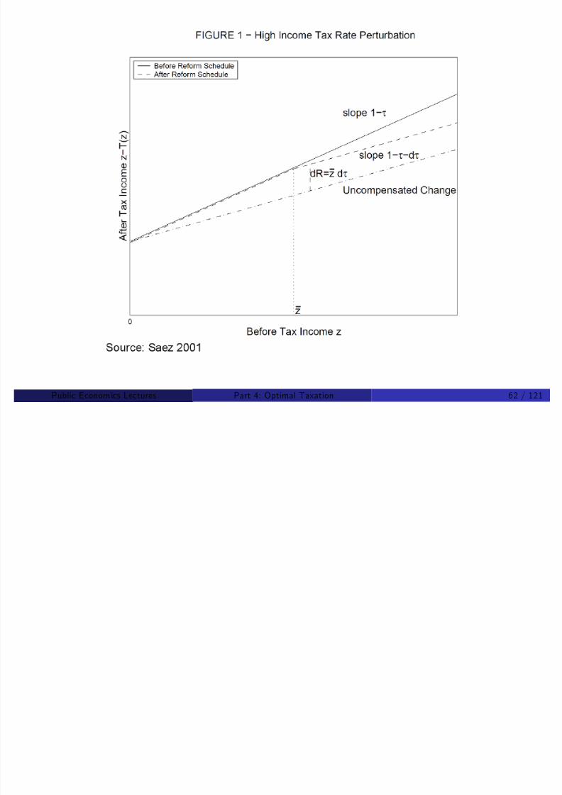
8/8/2019 Chetty - Public Economics Lectures
http://slidepdf.com/reader/full/chetty-public-economics-lectures 336/949
Public Econom ics Lectures () Part 4: Optimal Taxation 62 / 121
Optimal Top Income Tax Rate
Three e¤ects of small d τ > 0 reform above z
Mechanical increase in tax revenue:
dM = N [z m z ]d τ
Behavioral response:
dB = N τ dz m = N τ dz m
d (1 τ )d τ
= N τ
1 τ ε z m d τ
Welfare e¤ect: money-metric utility loss is dM by envelope theorem:
If govt. values marginal consumption of rich at g 2 (0, 1)
dW = g dM

8/8/2019 Chetty - Public Economics Lectures
http://slidepdf.com/reader/full/chetty-public-economics-lectures 337/949
dW = g dM
g depends on curvature of u (c ) and SWF
Public Econom ics Lectures () Part 4: Optimal Taxation 63 / 121
Optimal Top Income Tax Rate
dM + dW + dB = Nd τ (1 g )[z m z ] ε τ 1 τ
z mOptimal τ such that dM + dW + dB = 0 )
τ
TOP1 τ TOP
= (1 g
)(z
m/z
1)ε z m/z
τ TOP decreases with g [redistributive tastes]
τ TOP decreases with ε [e¢ciency]
τ TOP increases with z m/z [thickness of top tail]
/

8/8/2019 Chetty - Public Economics Lectures
http://slidepdf.com/reader/full/chetty-public-economics-lectures 338/949
Note: this is not an explicit formula for top tax rate because z m/z is
a fn. of τ
Public Econom ics Lectures () Part 4: Optimal Taxation 64 / 121

8/8/2019 Chetty - Public Economics Lectures
http://slidepdf.com/reader/full/chetty-public-economics-lectures 339/949
Public Econom ics Lectures () Part 4: Optimal Taxation 65 / 121
Optimal Top Income Tax Rate
In US tax return data, z m/z very stable above z = $200K withz mz
= 2
With Pareto distribution (f (z ) = a k a/z 1+a), aa1 = z m
z ) a = 2
) τ TOP =1 g
1 g + a ε
Ex: ε = 0.5, g = 0.5, a = 2 ) τ TOP = 33%

8/8/2019 Chetty - Public Economics Lectures
http://slidepdf.com/reader/full/chetty-public-economics-lectures 340/949
Public Econom ics Lectures () Part 4: Optimal Taxation 66 / 121
Zero Top Rate with Bounded Distribution
Suppose top earner earns z T
, and second earner earns z S
Then z m = z T when z > z S ) z m/z ! 1 when z ! z T )
dM = Nd τ [z m z ] ! 0 < dB = Nd τ ετ
1 τ
z m
Optimal τ is zero for z close to z T
Sadka-Seade zero top rate result
Result applies literally only to top earner: if z T = 2 z S thenz m/z = 2 when z = z S

8/8/2019 Chetty - Public Economics Lectures
http://slidepdf.com/reader/full/chetty-public-economics-lectures 341/949
Zero at top no longer considered to be of practical relevance
Public Econom ics Lectures () Part 4: Optimal Taxation 67 / 121
Connection to Revenue Maximizing Tax Rate
Revenue maximizing top tax rate can be calculated by putting 0weight on welfare of top incomes
Utilitarian SWF ) g = u c (z m ) ! 0 when z ! ∞
Rawlsian SWF ) g = 0 for any z > min(z )
If g = 0, we obtain τ TOP = τ MAX = 1/(1 + a ε)
Example: a = 2 and ε = 0.5 ) τ = 50%
La¤er linear rate is a special case where z = 0
) z m/z = ∞ = a/(a 1) ) a = 1 ) τMAX = 1/(1 + ε)
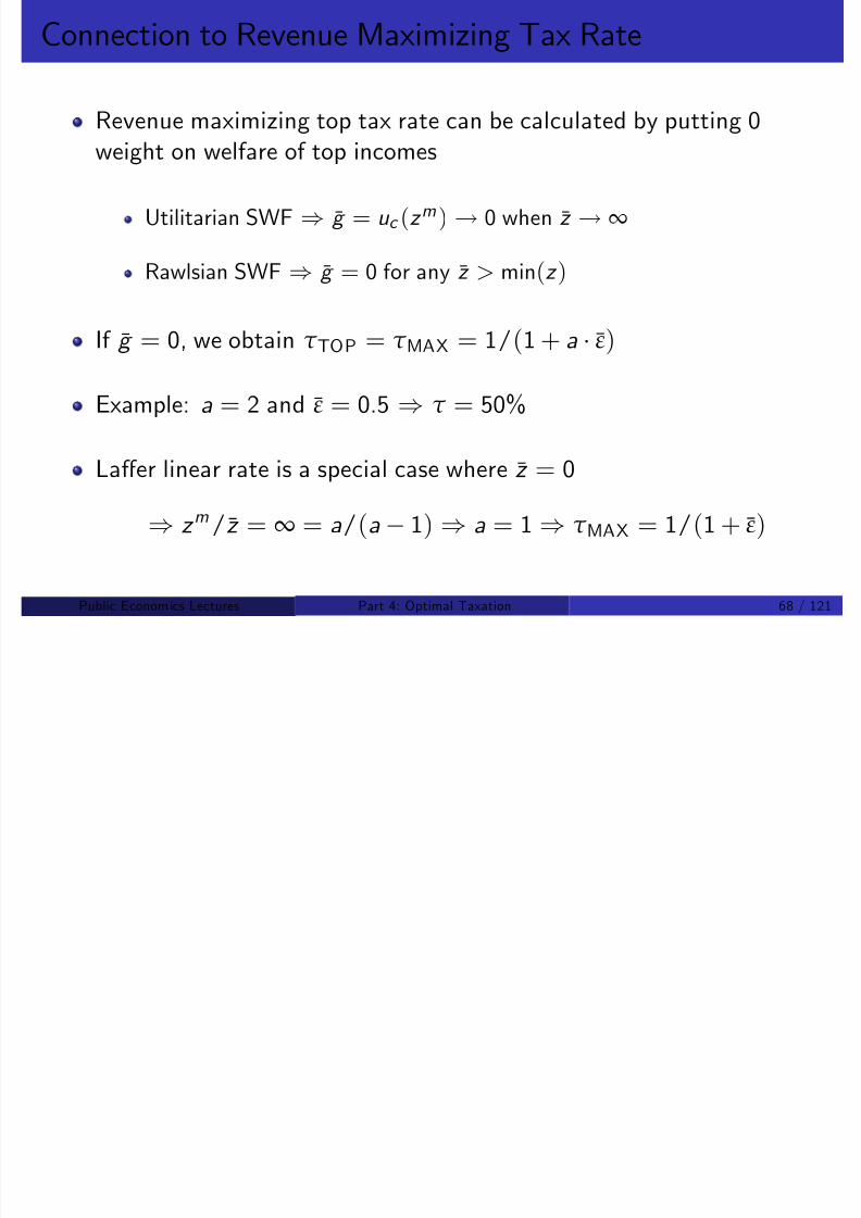
8/8/2019 Chetty - Public Economics Lectures
http://slidepdf.com/reader/full/chetty-public-economics-lectures 342/949
) z /z ∞ a/(a 1) ) a 1 ) τ MAX 1/(1 + ε)
Public Econom ics Lectures () Part 4: Optimal Taxation 68 / 121
Optimal Non-Linear Income Tax
Now consider general problem of setting optimal T (z )
Let H (z ) = CDF of income [population normalized to 1] and h(z ) its
density [endogenous to T (.)]
Let g (z ) = social marginal value of consumption for taxpayers withincome z in terms of public funds
Let G (z ) be the average social marginal value of consumption fortaxpayers with income above z [G (z ) =
R ∞z
g (s )h(s )ds /(1H (z ))]
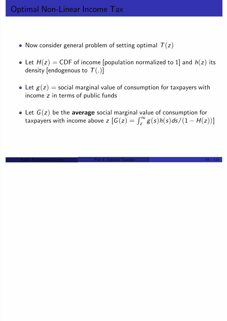
8/8/2019 Chetty - Public Economics Lectures
http://slidepdf.com/reader/full/chetty-public-economics-lectures 343/949
Public Econom ics Lectures () Part 4: Optimal Taxation 69 / 121

8/8/2019 Chetty - Public Economics Lectures
http://slidepdf.com/reader/full/chetty-public-economics-lectures 344/949
Public Econom ics Lectures () Part 4: Optimal Taxation 70 / 121
General Non-Linear Income Tax
Consider small reform: increase T 0 by d τ in small band (z , z + dz )
Mechanical revenue e¤ect
dM = dzd τ (1H (z ))
Mechanical welfare e¤ect
dW = dzd τ (1H (z ))G (z )
Behavioral e¤ect: substitution e¤ect δz inside small band [z , z + dz ]:
dB = h(z )dz T 0 δz = h(z )dz T 0 d τ ε(z ) z /(1 T 0)
Optimum dM + dW + dB = 0
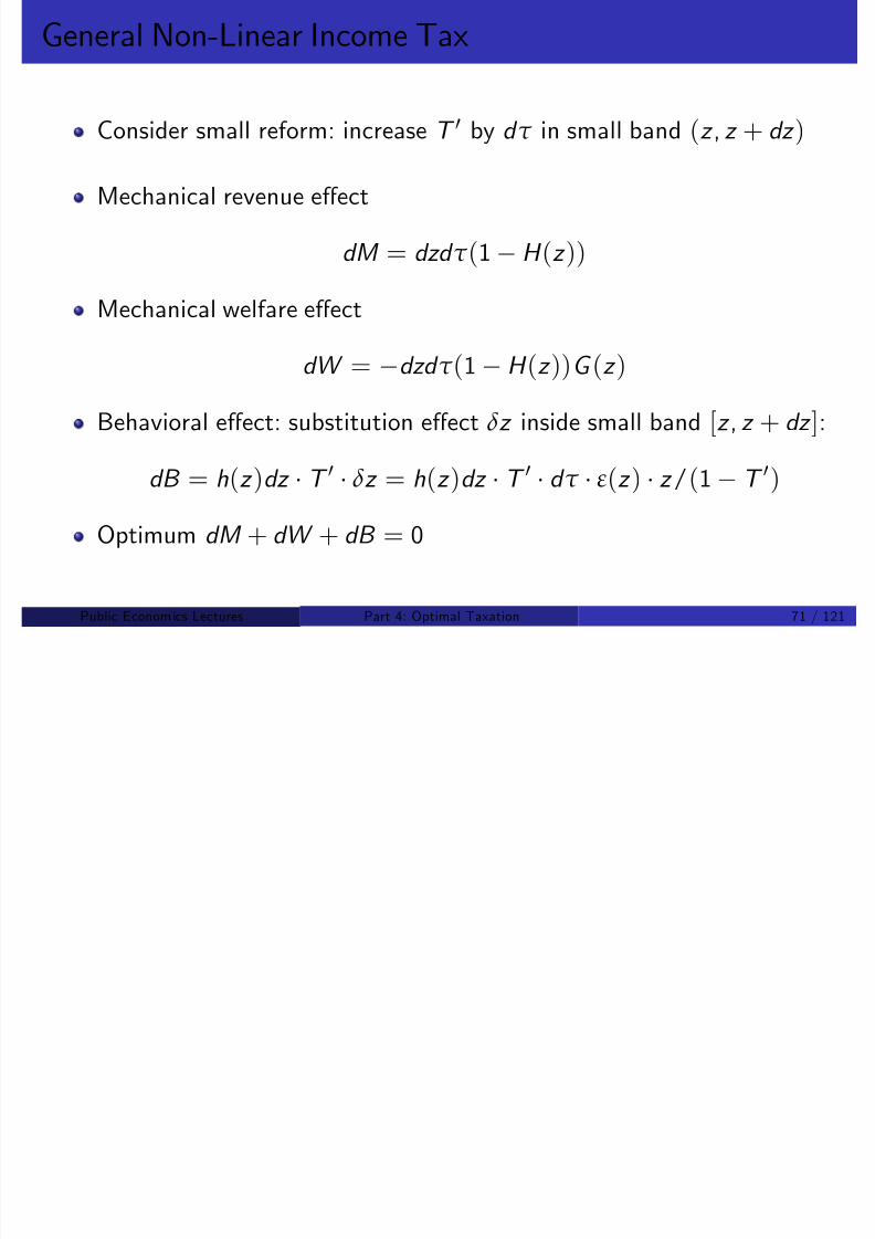
8/8/2019 Chetty - Public Economics Lectures
http://slidepdf.com/reader/full/chetty-public-economics-lectures 345/949
p + +
Public Econom ics Lectures () Part 4: Optimal Taxation 71 / 121
General Non-Linear Income Tax
Optimal tax schedule satis…es:
T 0(z )
1 T 0(z )=
1
ε(z )
1H (z )
zh(z )
[1 G (z )]
T 0
(z
) decreasing ing
(z 0
) forz 0 > z
[redistributive tastes]
T 0(z ) decreasing in ε(z ) [e¢ciency]
T 0(z ) decreasing in h(z )/(1H (z )) [density]
Connection to top tax rate: consider z ! ∞
G (z ) ! g , (1H (z ))/(zh(z )) ! 1/a

8/8/2019 Chetty - Public Economics Lectures
http://slidepdf.com/reader/full/chetty-public-economics-lectures 346/949
ε(z ) ! ε ) T 0(z ) = (1 g )/(1 g + a ε) = τ TOP
Public Econom ics Lectures () Part 4: Optimal Taxation 72 / 121
Negative Marginal Tax Rates Never Optimal
Suppose T 0 < 0 in band [z , z + dz ]
Increase T 0 by d τ > 0 in band [z , z + dz ]
dM + dW > 0 because G (z ) < 1 for any z > 0 (with declining g (z )and G (0) = 1)dB > 0 because T 0(z ) < 0 [smaller e¢ciency cost]
Therefore T 0(z ) < 0 cannot be optimal
Marginal subsidies also distort local incentives to work
Better to redistribute using lump sum grant

8/8/2019 Chetty - Public Economics Lectures
http://slidepdf.com/reader/full/chetty-public-economics-lectures 347/949
Public Econom ics Lectures () Part 4: Optimal Taxation 73 / 121
Numerical Simulations of Optimal Tax Schedule
Formula above is a condition for optimality but not an explicitformula for optimal tax schedule
Distribution of incomes H (z ) endogenous to T (.)
Therefore need to use structural approach (speci…cation of primitives)to calculate optimal T (.)
Saez (2001) speci…es utility function (e.g. constant elasticity):
u (c , l ) = c (l )1+ 1ε
) l = [(1 T 0)w ]ε
Calibrate the exogenous skill distribution F (w ) such that actual T (.)

8/8/2019 Chetty - Public Economics Lectures
http://slidepdf.com/reader/full/chetty-public-economics-lectures 348/949
yields empirical H (z )Public Econom ics Lectures () Part 4: Optimal Taxation 74 / 121

8/8/2019 Chetty - Public Economics Lectures
http://slidepdf.com/reader/full/chetty-public-economics-lectures 349/949
Public Econom ics Lectures () Part 4: Optimal Taxation 75 / 121
Numerical Simulations
Use formula expressed in terms of F (w ) to solve for optimal T (z ):
T 0(z (w ))
1 T 0(z (w ))=
1 +
1
ε
1
wf (w )
Z ∞w
1
G 0(u (s ))
p
f (s )ds ,
where p = R G 0(u (s ))f (s )ds is marginal value of public funds
Iterative …xed point method to solve for T (z ):
Start with initial MTR schedule T 00 and compute incomes z 0(w ) usingindividual FOCs
Get T 0(0) using govt budget constraint, compute utilities u 0(w )
Compute p 0 =R
G 0(u 0(s ))f (s )ds
Use formula to calculate T 01 and iterate until convergence (Brewer,
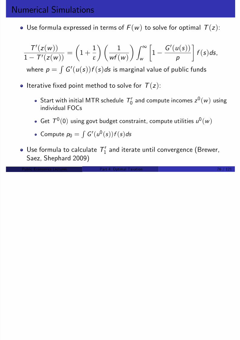
8/8/2019 Chetty - Public Economics Lectures
http://slidepdf.com/reader/full/chetty-public-economics-lectures 350/949
Use formula to calculate T 1 and iterate until convergence (Brewer,
Saez, Shephard 2009)
Public Econom ics Lectures () Part 4: Optimal Taxation 76 / 121

8/8/2019 Chetty - Public Economics Lectures
http://slidepdf.com/reader/full/chetty-public-economics-lectures 351/949
Public Econom ics Lectures () Part 4: Optimal Taxation 77 / 121
Commodity vs. Income Taxation
Now combine commodity tax and income tax results to analyzeoptimal combination of policies
In practice, government levies di¤erential commodity taxes along withnon-linear income tax
1 Exempts some goods (food, education, health) from sales tax
2 Imposes additional excise taxes on some goods (cars, gasoline, luxury
goods)
3 Imposes capital income taxes
What is the best combination of taxes?
8/8/2019 Chetty - Public Economics Lectures
http://slidepdf.com/reader/full/chetty-public-economics-lectures 352/949
Public Econom ics Lectures () Part 4: Optimal Taxation 78 / 121
Commodity vs. Income Taxation: Model
K consumption goods c = (c 1, .., c K ) with pre-tax pricep = (p 1, .., p K )
Individual h has utility u h (c 1, .., c K , z )
Can govt increase welfare using commodity taxes t = (t 1, .., t K ) inaddition to nonlinear optimal income tax on earnings z ?
We know that more instruments cannot hurt:
maxt ,T (.)
SWF maxt =0,T (.)
SWF

8/8/2019 Chetty - Public Economics Lectures
http://slidepdf.com/reader/full/chetty-public-economics-lectures 353/949
Public Econom ics Lectures () Part 4: Optimal Taxation 79 / 121
Atkinson and Stiglitz: Commodity Taxation is Super‡uous
Atkinson and Stiglitz (1976) show that
maxt ,T (.)
SWF = maxt =0,T (.)
SWF
Commodity taxes not useful under two assumptions on utility
functions u h
(c 1, .., c K , z )
1 Separability between (c 1, .., c K ) and z in utility
2 Homogeneity across individuals in the sub-utility of consumption:
u h (c 1, .., c K , z ) = U h (v (c 1, .., c K ), z )
Original proof was based on optimality conditions

8/8/2019 Chetty - Public Economics Lectures
http://slidepdf.com/reader/full/chetty-public-economics-lectures 354/949
More straightforward proof by Laroque (2005) and Kaplow (2006)
Public Econom ics Lectures () Part 4: Optimal Taxation 80 / 121
Atkinson-Stiglitz: Proof
Let V (y , q ) = maxc v (c 1, .., c K ) st qc y be the indirect utility of consumption given post-tax earnings y and price q
This function is common across all individuals under assumptions above
Start with any tax system (T (.), t )
Replace (T (.), t ) with (T (.), t = 0) where T (z ) is such that
V (z T (z ), p + t ) = V (z T (z ), p )
Utility U h(V , z ) unchanged for all individuals
Labor supply choices z unchanged as well because return to workV 0 z

8/8/2019 Chetty - Public Economics Lectures
http://slidepdf.com/reader/full/chetty-public-economics-lectures 355/949
V (
z ) unchanged
Public Econom ics Lectures () Part 4: Optimal Taxation 81 / 121
Atkinson-Stiglitz: Proof
Revenue under original tax system: T (z ) + t c (t )
Revenue under new tax system: T (z )
Claim: T (z ) T (z ) + t c (t )
Conditional on z , T (z ) is a lump sum tax whereas t is distortionary
For a given utility level, can extract more using lump sum tax thandistortionary tax

8/8/2019 Chetty - Public Economics Lectures
http://slidepdf.com/reader/full/chetty-public-economics-lectures 356/949
Public Econom ics Lectures () Part 4: Optimal Taxation 82 / 121
Atkinson-Stiglitz: Proof
Algebraic proof of claim
Let c (t ) denote optimal bundle with tax (t , T (z )) and c (0) denoteoptimal bundle with tax (0, T (z ))
Both bundles yield same utilityV
by construction
Optimization implies
p c (t ) = z T (z ) t c (t ) p c (0) = z T (z )
) T (z ) T (z ) + t c (t )
Government collects more taxes with (T (.), t = 0) and utility isunchanged
Therefore system without commodity taxes yields higher welfare

8/8/2019 Chetty - Public Economics Lectures
http://slidepdf.com/reader/full/chetty-public-economics-lectures 357/949
Therefore system without commodity taxes yields higher welfare
Public Econom ics Lectures () Part 4: Optimal Taxation 83 / 121
Atkinson-Stiglitz: Intuition
With separability and homogeneity, conditional on earnings z ,consumption choices c = (c 1, .., c K ) do not provide any informationon ability
Di¤erentiated commodity taxes t 1, .., t K create a tax distortion with
no bene…t
Better to do all the redistribution with the individual income tax
With only linear income taxation (Diamond-Mirrlees 1971, Diamond1975), di¤. commodity taxation can be useful to “non-linearize” thetax system
But not if Engel curves for each c k are linear in y (Deaton 1981)
8/8/2019 Chetty - Public Economics Lectures
http://slidepdf.com/reader/full/chetty-public-economics-lectures 358/949
Public Econom ics Lectures () Part 4: Optimal Taxation 84 / 121
Failures of A-S Assumptions
If higher ability consume more of good k than lower ability people,then taxing good k is desirable. Examples:
1 High ability people have a relatively higher taste for good k (at a givenincome)
Luxury chocolates or museums; violates homogeneous v (c ) assumption
2 Good k is positively related to leisure (consumption of k increaseswhen leisure increases at a given income)
Tax on travel, subsidy on computers and work related expenses
In general Atkinson-Stiglitz assumptions are viewed as a good starting
8/8/2019 Chetty - Public Economics Lectures
http://slidepdf.com/reader/full/chetty-public-economics-lectures 359/949
place for most goodsPublic Econom ics Lectures () Part 4: Optimal Taxation 85 / 121
Atkinson-Stiglitz: Implications for Capital Taxation
Two period model: wage rate w in period 1, retired in period 2
Let δ = discount rate, ψ(.) disutility of e¤ort, and utility
u h (c 1, c 2, z ) = u (c 1) +u (c 2)
1 + δ ψ(z /w )
The budget constraint is
c 1 + c 2/(1 + r (1 t K )) z T (z )
Tax on savingst
K is equivalent to tax onc
2
Atkinson-Stiglitz implies that t K = 0 in the presence of an optimalincome tax
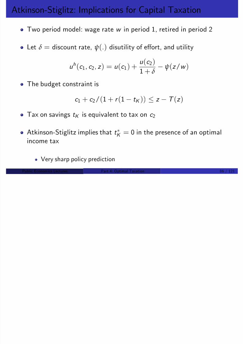
8/8/2019 Chetty - Public Economics Lectures
http://slidepdf.com/reader/full/chetty-public-economics-lectures 360/949
Very sharp policy prediction
Public Econom ics Lectures () Part 4: Optimal Taxation 86 / 121
Atkinson-Stiglitz: Implications for Capital Taxation
If low ability people have higher δ then capital income tax t K > 0 isdesirable (Saez 2004)
Violates homogeneous utility assumption
Savings are equivalent to luxury chocolates or museums
Saez (2004) restricts capital tax to be linear and income-independent
With non-linear, income-dependent taxes, optimal t K may be lower forhigh incomes than low incomes (Golosov, Tsyvinski, Weinzierl 2009)
No longer a justi…cation for redistribution via capital income taxation
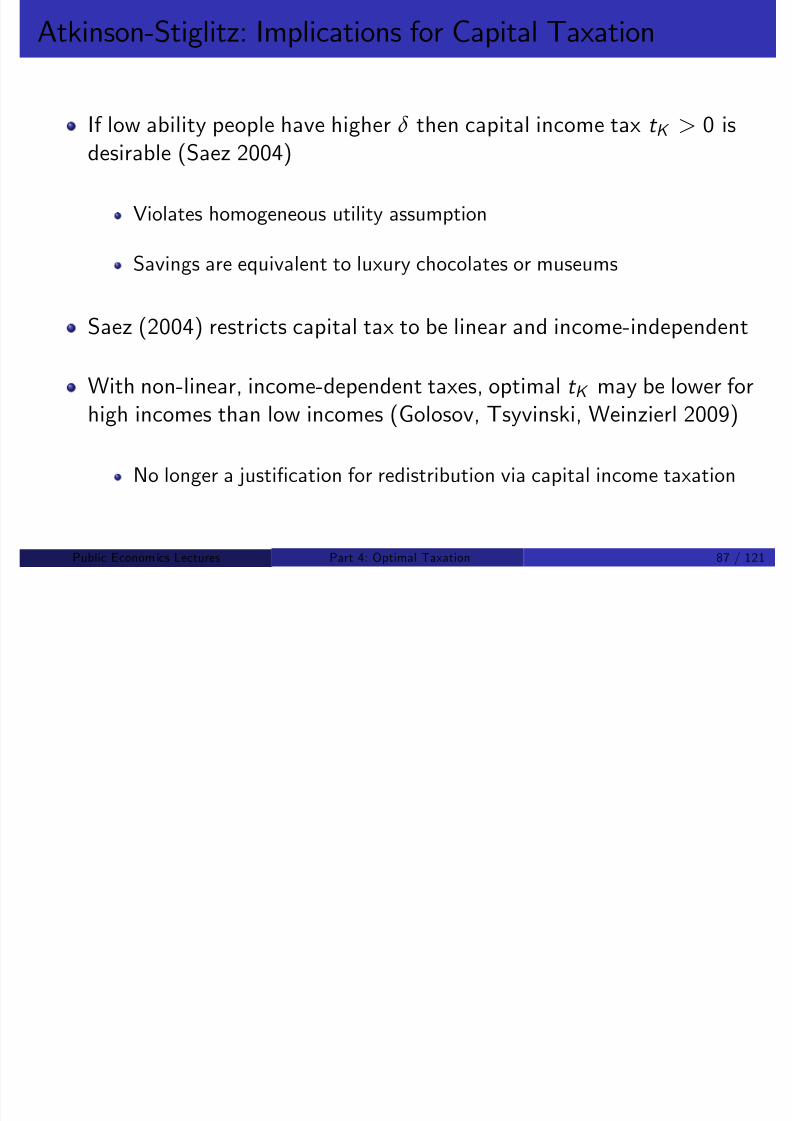
8/8/2019 Chetty - Public Economics Lectures
http://slidepdf.com/reader/full/chetty-public-economics-lectures 361/949
Public Econom ics Lectures () Part 4: Optimal Taxation 87 / 121
Chamley-Judd: Capital Taxation
Judd (1985) and Chamley (1986) give a di¤erent argument againstcapital taxation
Consider a Ramsey model where govt. is limited to lineardistortionary taxes
Result: optimal capital tax converges to zero in long run
Intuition: DWL rises with square of tax rate
With non-zero capital tax, have an in…nite price distortion between c 0and c t as t ! ∞
Undesirable to have such large distortions on some margins
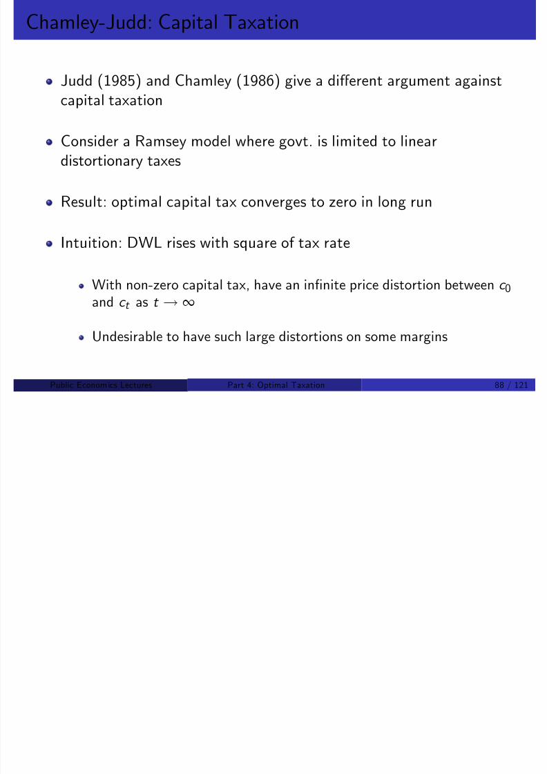
8/8/2019 Chetty - Public Economics Lectures
http://slidepdf.com/reader/full/chetty-public-economics-lectures 362/949
Public Econom ics Lectures () Part 4: Optimal Taxation 88 / 121
Chamley-Judd vs. Atkinson-Stiglitz
Chamley-Judd: constrained policy instruments (linear taxes) but
dynamic
Atkinson-Stiglitz: full set of policy instruments (non linear incometax) but static
New dynamic public …nance literature: full set of instruments indynamic model
Key result: in dynamic Mirrlees models, optimal capital tax is notzero (Golosov, Kocherlekota, and Tsyvinski 2003)
Optimum satis…es Inverse Euler eqn., resulting in a wedge betweenMRS and MRTS
Intuition: payo¤ to distorting savings decisions relaxes IC constraints inoptimal income tax problem in next period
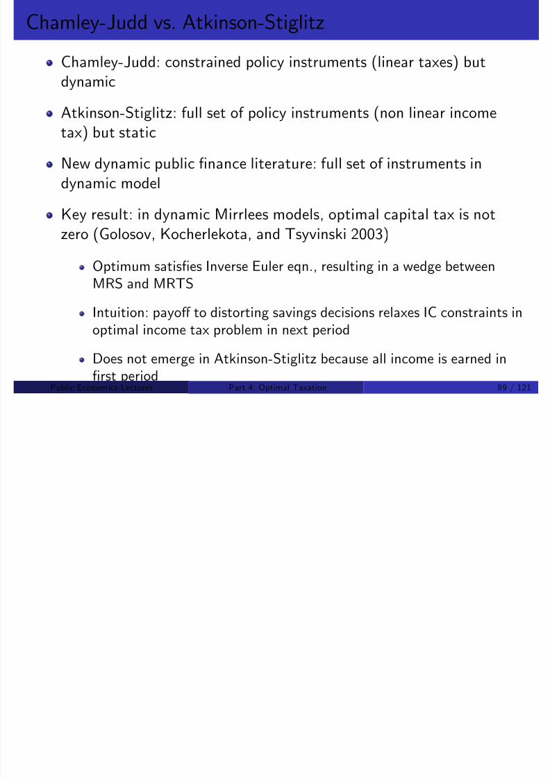
8/8/2019 Chetty - Public Economics Lectures
http://slidepdf.com/reader/full/chetty-public-economics-lectures 363/949
Does not emerge in Atkinson-Stiglitz because all income is earned in…rst period
Public Econom ics Lectures () Part 4: Optimal Taxation 89 / 121
Taxation and Savings: Evidence
Key assumption in Chamley-Judd and Atkinson-Stiglitz results:people optimize their savings decisions
Recent evidence challenges this assumption
Madrian and Shea (2001) study employee 401(k) enrollment decisionsand contribution rates at a U.S. corporation:
Most people adhere to company defaults and do not make active
savings choices
Suggests that defaults may have much bigger impacts on savingsdecision than net-of-tax returns
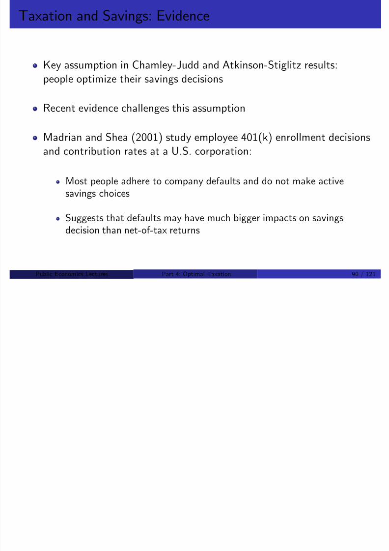
8/8/2019 Chetty - Public Economics Lectures
http://slidepdf.com/reader/full/chetty-public-economics-lectures 364/949
Public Econom ics Lectures () Part 4: Optimal Taxation 90 / 121
Madrian and Shea 2001: Defaults and Savings Behavior

8/8/2019 Chetty - Public Economics Lectures
http://slidepdf.com/reader/full/chetty-public-economics-lectures 365/949
Public Econom ics Lectures () Part 4: Optimal Taxation 91 / 121

8/8/2019 Chetty - Public Economics Lectures
http://slidepdf.com/reader/full/chetty-public-economics-lectures 366/949
Public Econom ics Lectures () Part 4: Optimal Taxation 92 / 121

8/8/2019 Chetty - Public Economics Lectures
http://slidepdf.com/reader/full/chetty-public-economics-lectures 367/949
Public Econom ics Lectures () Part 4: Optimal Taxation 93 / 121
Optimal Transfer Programs
Several types of transfer programs are used in practice, each justi…edby a di¤erent theory and set of assumptions
Option 1: Negative Income Tax: TANF (Mirrlees 1971)
Bene…ts: no one omitted; low admin costs; no stigma
Costs: e¢ciency loss from less work
Option 2: Work-for-welfare: EITC (Saez 2002)
Bene…ts: more incentive to work; low admin costs
Costs: e¢ciency loss in phaseout range, no coverage of non-workers

8/8/2019 Chetty - Public Economics Lectures
http://slidepdf.com/reader/full/chetty-public-economics-lectures 368/949
Public Econom ics Lectures () Part 4: Optimal Taxation 94 / 121
Optimal Transfer Programs
Option 3: Categorical anti-poverty programs: assistance for blind(Akerlof 1978)
Bene…ts: tagging relaxes incentive constraint by tying tax rate toimmutable qualities
Costs: not always feasible and limited coverage
Option 4: In-kind transfers: food stamps, public housing (Nicholsand Zeckhauser 1982)
Bene…ts: E¢ciency gains from relaxing IC for high-types via ordeals
Costs: Paternalism (spend on the right things), ine¢cient ordeal cost
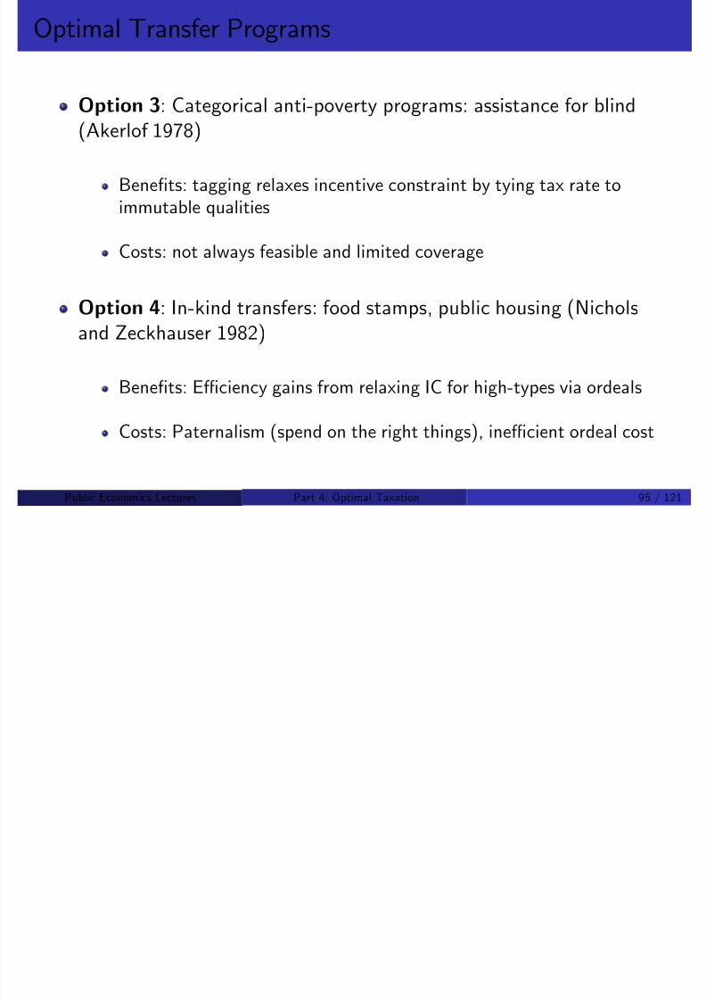
8/8/2019 Chetty - Public Economics Lectures
http://slidepdf.com/reader/full/chetty-public-economics-lectures 369/949
Public Econom ics Lectures () Part 4: Optimal Taxation 95 / 121
Optimal Transfers: Mirrless Model
Mirrlees model predicts that optimal transfer at bottom takes theform of a Negative Income Tax
Lump sum grant T (0) for those with no earnings
High MTRs T 0(z ) at the bottom to phase-out the lumpsum grantquickly
Intuition: NIT optimal because
Targets transfers to the most needy
Earnings at the bottom are low to start with so intensive response tohigh MTRs does not generate large output losses

8/8/2019 Chetty - Public Economics Lectures
http://slidepdf.com/reader/full/chetty-public-economics-lectures 370/949
Public Econom ics Lectures () Part 4: Optimal Taxation 96 / 121
Optimal Transfers: Participation Responses and EITC
Mirrlees result predicated on assumption that all individuals are at aninterior optimum in choice of labor supply
Rules out extensive-margin responses
But empirical literature shows that participation labor supply responsesare most important especially for low incomes
Diamond (1980), Saez (2002), Laroque (2005) incorporate such
extensive labor supply responses into optimal income tax model
Generate extensive margin by introducing …xed job packages (cannotsmoothly choose earnings)

8/8/2019 Chetty - Public Economics Lectures
http://slidepdf.com/reader/full/chetty-public-economics-lectures 371/949
Public Econom ics Lectures () Part 4: Optimal Taxation 97 / 121
Saez 2002: Participation Model
Model with discrete earnings outcomes: w 0
= 0 < w 1< ... < w I
Tax/transfer T i when earning w i , c i = w i T i
Pure participation choice: skill i individual compares c i and c 0 when
deciding to work
With participation tax rate τ i , c i c 0 = w i (1 τ i )
In aggregate, fraction hi (c i c 0
) of population earns w i , so ∑ i
hi = 1
Participation elasticity is
e i = (c i c 0)/hi ∂hi /∂(c i c 0)

8/8/2019 Chetty - Public Economics Lectures
http://slidepdf.com/reader/full/chetty-public-economics-lectures 372/949
Public Econom ics Lectures () Part 4: Optimal Taxation 98 / 121
Saez 2002: Participation Model
Social Welfare function is summarized by social marginal welfareweights at each earnings level g i
No income e¤ects ! ∑ i g i hi = 1
Main result: work subsidies with T 0(z ) < 0 (such as EITC) optimal
Key requirements in general model with intensive+extensive responses
Responses are concentrated primarily along extensive margin
Social marginal welfare weight on low skilled workers > 1
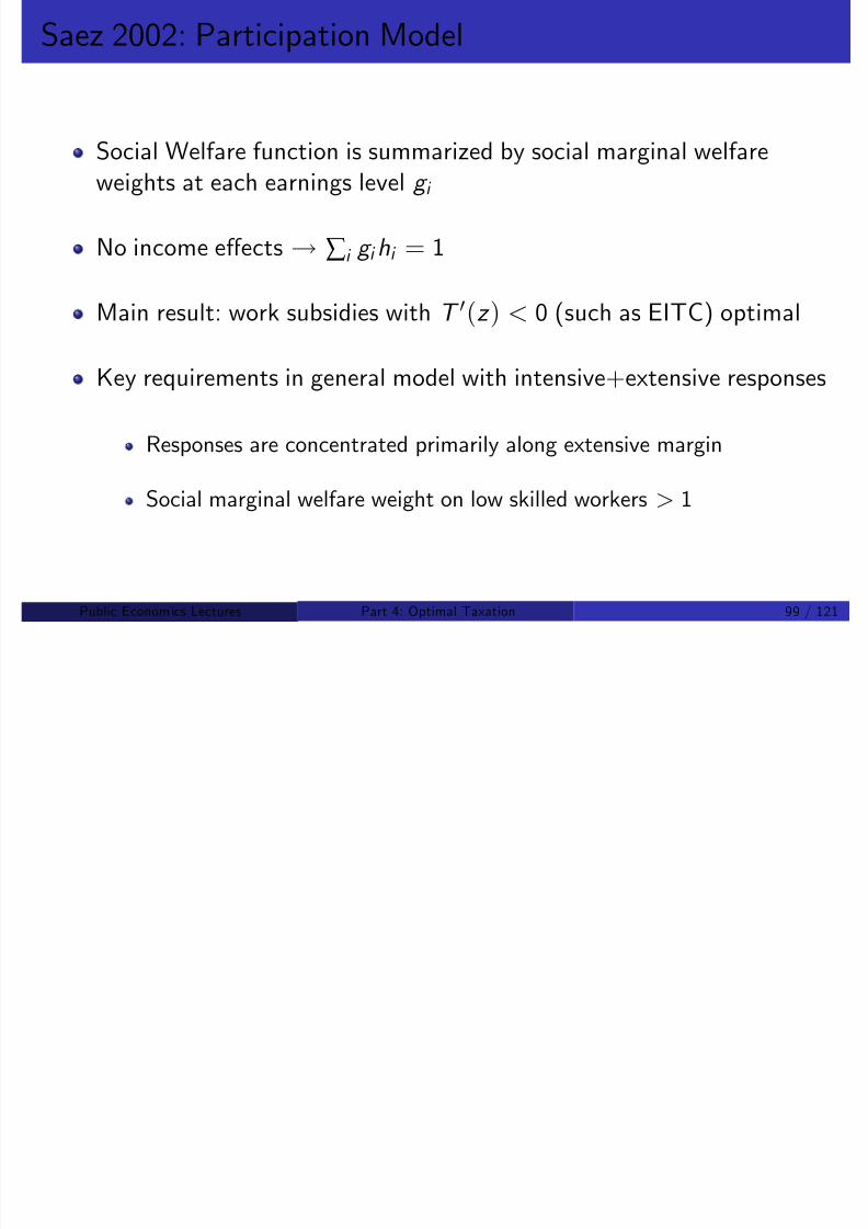
8/8/2019 Chetty - Public Economics Lectures
http://slidepdf.com/reader/full/chetty-public-economics-lectures 373/949
Public Econom ics Lectures () Part 4: Optimal Taxation 99 / 121

8/8/2019 Chetty - Public Economics Lectures
http://slidepdf.com/reader/full/chetty-public-economics-lectures 374/949
Public Econom ics Lectures () Part 4: Optimal Taxation 100 / 121

8/8/2019 Chetty - Public Economics Lectures
http://slidepdf.com/reader/full/chetty-public-economics-lectures 375/949
Public Econom ics Lectures () Part 4: Optimal Taxation 101 / 121

8/8/2019 Chetty - Public Economics Lectures
http://slidepdf.com/reader/full/chetty-public-economics-lectures 376/949
Public Econom ics Lectures () Part 4: Optimal Taxation 102 / 121
Mirrlees 1971 vs. Saez 2002
EITC is desirable in Saez extensive-margin model because it
Redistributes more money to low incomes
Saves the government money by getting people o¤ of welfare
In Mirrlees intensive-margin model, second e¤ect is shut down
Creating an EITC would always cost government more throughintensive responses
Always preferable to redistribute by giving more money to lowestincome

8/8/2019 Chetty - Public Economics Lectures
http://slidepdf.com/reader/full/chetty-public-economics-lectures 377/949
Public Econom ics Lectures () Part 4: Optimal Taxation 103 / 121
Saez 2002: Optimal Tax Formula
Small reform dc i = dT i > 0. Three e¤ects:
1 Mechanical loss of tax revenue dM = hi dT i
2 Welfare E¤ect: each worker in job i gains dT i so welfare gaindW = g i hi dT i
No …rst order welfare loss for switchers
3 Behavioral E¤ect: dhi = e i hi dT i /(c i c 0)!Tax loss: dB = (T i T 0)dhi = e i hi dT i (T i T 0)/(c i c 0)
FOC: dM + dB + dW = 0 )
τ i 1 τ i
=T i T 0
c i c 0=
1
e i (1 g i )
g1 > 1 ) T1 T0 < 0 ) work subsidy
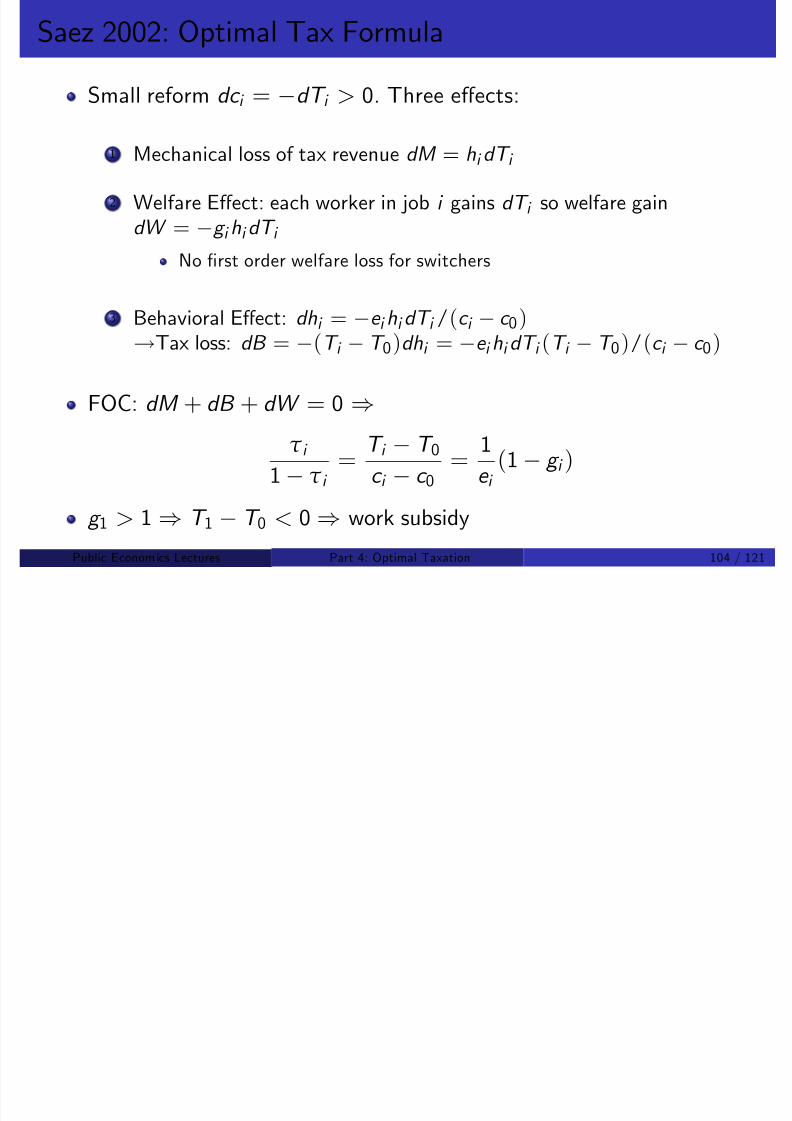
8/8/2019 Chetty - Public Economics Lectures
http://slidepdf.com/reader/full/chetty-public-economics-lectures 378/949
g 1 ) T T 0 ) work subsidyPublic Econom ics Lectures () Part 4: Optimal Taxation 104 / 121
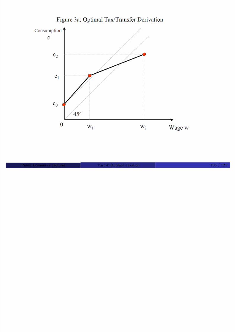
8/8/2019 Chetty - Public Economics Lectures
http://slidepdf.com/reader/full/chetty-public-economics-lectures 379/949
Public Econom ics Lectures () Part 4: Optimal Taxation 105 / 121

8/8/2019 Chetty - Public Economics Lectures
http://slidepdf.com/reader/full/chetty-public-economics-lectures 380/949
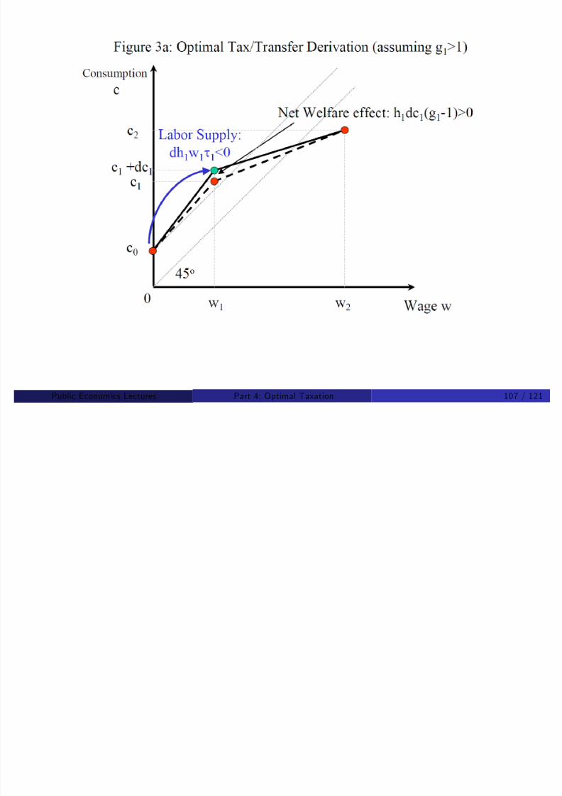
8/8/2019 Chetty - Public Economics Lectures
http://slidepdf.com/reader/full/chetty-public-economics-lectures 381/949
Public Econom ics Lectures () Part 4: Optimal Taxation 107 / 121

8/8/2019 Chetty - Public Economics Lectures
http://slidepdf.com/reader/full/chetty-public-economics-lectures 382/949
Public Econom ics Lectures () Part 4: Optimal Taxation 108 / 121
Saez 2002: General Model
Model can be extended to allow both intensive and extensiveresponses
Allow higher types to switch to lower jobs
General formula for optimal tax is a fn of both intensive and extensivemargin elasticity
Can be calibrated using empirical estimates of these elasticities

8/8/2019 Chetty - Public Economics Lectures
http://slidepdf.com/reader/full/chetty-public-economics-lectures 383/949
Public Econom ics Lectures () Part 4: Optimal Taxation 109 / 121

8/8/2019 Chetty - Public Economics Lectures
http://slidepdf.com/reader/full/chetty-public-economics-lectures 384/949
Public Econom ics Lectures () Part 4: Optimal Taxation 110 / 121
Tagging: Akerlof 1978
We have assumed that T (z ) depends only on earnings z
In reality, govt can observe many other characteristics X alsocorrelated with ability and set T (z , X )
Ex: gender, race, age, disability, family structure, height,...
Two major results:
1 If characteristic X is immutable then redistribution across the X
groups will be complete [until average social marginal welfare weightsare equated across X groups]
2 If characteristic X can be manipulated but X correlated with abilitythen taxes will depend on both X and z

8/8/2019 Chetty - Public Economics Lectures
http://slidepdf.com/reader/full/chetty-public-economics-lectures 385/949
Public Econom ics Lectures () Part 4: Optimal Taxation 111 / 121
Mankiw and Weinzierl 2009
Tagging with Immutable Characteristics
Consider a binary immutable tag: Tall vs. Short
1 inch = 2% higher earnings on average (Postlewaite et al. 2004)
Average social marginal welfare weights g T < g S because tall earn
more
Lump sum transfer from Tall to Short is desirable
Optimal transfer should be up to the point where g T = g S
Calibrations show that average tall person (> 6ft) should pay $4500more in tax

8/8/2019 Chetty - Public Economics Lectures
http://slidepdf.com/reader/full/chetty-public-economics-lectures 386/949
Public Econom ics Lectures () Part 4: Optimal Taxation 112 / 121
Problems with Tagging
Height taxes seem implausible, challenging validity of tagging model
What is the model missing?
1 Horizontal Equity concerns impose constraints on feasible policies:
Two people earning same amount but of di¤erent height should betreated the same way
2 Height does not cause high earnings
In practice, tags used only when causally related to ability to earn[disability status] or welfare [family structure, # kids, medical expenses]
Lesson: Mirrlees analysis [T (z )] may be most sensible even in an
environment with immutable tags()
/

8/8/2019 Chetty - Public Economics Lectures
http://slidepdf.com/reader/full/chetty-public-economics-lectures 387/949
Public Econom ics Lectures () Part 4: Optimal Taxation 113 / 121
Nichols and Zeckhauser 1982: In-Kind Redistribution
In …rst-best full information model, no reason for in-kind transfers
In-kind transfer is tradeable at market price ! in-kind equivalent tocash
In-kind transfer non-tradeable ! in-kind inferior to cash
Nichols and Zeckhauser: potential rationale for in-kind transfersemerges in Mirrlees-type model with informational constraints
With heterogeneity in preferences, may be able to relax IC constraintsusing in-kind transfers
P bli E i L ()
P 4 O i l T i 114 / 121

8/8/2019 Chetty - Public Economics Lectures
http://slidepdf.com/reader/full/chetty-public-economics-lectures 388/949
Public Econom ics Lectures () Part 4: Optimal Taxation 114 / 121
Nichols and Zeckhauser: Simple Illustration
Consider a soup kitchen as an in-kind transfer policy
Let S = soup and W = wait in minutes
Two agents: poor (P ) and rich (R )
Utility functions are increasing in S and decreasing in W :
U p = 2S .5W
U r = S 1W
R has higher disutility from waiting and lower utility from soup
Social welfareSWF = U p + U r
P bli E i L t ()
P t 4 O ti l T ti 115 / 121
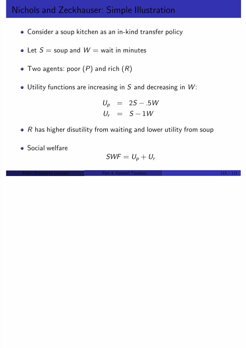
8/8/2019 Chetty - Public Economics Lectures
http://slidepdf.com/reader/full/chetty-public-economics-lectures 389/949
Public Econom ics Lectures () Part 4: Optimal Taxation 115 / 121
Soup Kitchen without Wait: Cash Transfer
With a total of $100 in soup to give away and no wait times, the soupwill be split between the two agents
Both get some utility from soup, so both will claim it
Assume that they split it equally, resulting in
U p = 100
U r = 50
SWF = 150
Equivalent to a cash-transfer program that pays each agent $50
Public Econom ics Lectures ()
Part 4: Optimal Taxation 116 / 121

8/8/2019 Chetty - Public Economics Lectures
http://slidepdf.com/reader/full/chetty-public-economics-lectures 390/949
Public Econom ics Lectures () Part 4: Optimal Taxation 116 / 121
Soup Kitchen with Wait Times: In-Kind Transfer
Now suppose we impose wait time of 51 minutes
R leaves - not worth it to him for $50 in food - gets U p = 0
P gets utility of 200 25.5 = 174.5
Social welfare with in-kind transfer (wait time) greater than cashtransfer (no wait time)
Targeting gains outweighing e¢ciency losses from ordeal
Scope for such targeting depends upon degree of heterogeneity inpreferences
Public Econom ics Lectures ()
Part 4: Optimal Taxation 117 / 121
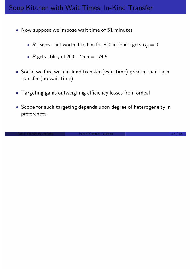
8/8/2019 Chetty - Public Economics Lectures
http://slidepdf.com/reader/full/chetty-public-economics-lectures 391/949
Public Econom ics Lectures () Part 4: Optimal Taxation 117 / 121
Income Taxation as Insurance (Varian 1980)
Important limitiation of Mirrlees model: no ex-post uncertainty
Once skill type is revealed, agent controls income perfectly
In practice, there is considerable ex-post uncertainty in incomes (e.g.unemployment shocks)
In this case, a progressive tax system could provide insurance
Do not want 100% insurance for moral hazard reasons
But some insurance desirable if individuals are risk averse
Public Econom ics Lectures ()
Part 4: Optimal Taxation 118 / 121

8/8/2019 Chetty - Public Economics Lectures
http://slidepdf.com/reader/full/chetty-public-economics-lectures 392/949
Public Econom ics Lectures () Part 4: Optimal Taxation 118 / 121
Varian: Taxation as Insurance
Income z = e + where e is e¤ort and is a random noise
Government observes only z and sets a tax schedule based on z
Individual utilityU = Eu (z T (z )) e
Chooses e = e to maximize this utility
E¤ort e low if tax schedule very redistributive
Government chooses T (.) to maximize indirect utility: trade-o¤ insurance vs incentives
Optimal tax system depends on parameters similar to those in
Mirrlees modelPublic Econom ics Lectures ()
Part 4: Optimal Taxation 119 / 121

8/8/2019 Chetty - Public Economics Lectures
http://slidepdf.com/reader/full/chetty-public-economics-lectures 393/949
Public Econom ics Lectures () Part 4: Optimal Taxation 119 / 121
Varian Model: Private Insurance
Varian model has received less attention than Mirrlees model
One reason: government is not better than private market inproviding such insurance
In adverse selection (e.g. Mirrlees) models, only government canimprove redistributive outcomes once skills are revealed to agents
Agents cannot write contracts behind veil of ignorance
In pure moral hazard model with ex-post information revelation,private markets should in principle reach optimum themselves
In practice, …rms o¤er wage contracts that provide some insuranceagainst bad luck
Ex: tenure system in universities, increase of pay with job tenure,
severance paymentsPublic Econom ics Lectures ()
Part 4: Optimal Taxation 120 / 121

8/8/2019 Chetty - Public Economics Lectures
http://slidepdf.com/reader/full/chetty-public-economics-lectures 394/949
() p /
Income Taxation and Social Insurance
Two potential approaches to addressing private insurance provision
1 Optimal taxation with endogenous private insurance
Not clear how to model and measure endogenous private insurance
See Golosov and Tsyvinski (2007) and Chetty and Saez (2009) forsome attempts
2 Focus on speci…c shocks where private markets are thought to bequite limited
Unemployment, disability, injury on the job
Not just general insurance against wage earnings ‡uctuations
Motivates literature on optimal social insurancePublic Econom ics Lectures ()
Part 4: Optimal Taxation 121 / 121

8/8/2019 Chetty - Public Economics Lectures
http://slidepdf.com/reader/full/chetty-public-economics-lectures 395/949
() p /
Public Economics LecturesPart 5: Income Taxation and Labor Supply
Raj Chetty and Gregory A. Bruich
Harvard University
Fall 2009
Public Economics Lectures ()
Part 5: Income Taxation and Labor Supply 1 / 211

8/8/2019 Chetty - Public Economics Lectures
http://slidepdf.com/reader/full/chetty-public-economics-lectures 396/949

8/8/2019 Chetty - Public Economics Lectures
http://slidepdf.com/reader/full/chetty-public-economics-lectures 397/949
References
Surveys in labor economics:
Pencavel (1986) Handbook of Labor Economics vol 1
Heckman and Killingsworth (1986) Handbook of Labor Econ vol 1
Blundell and MaCurdy (1999) Handbook of Labor Economics vol 3
Surveys in public economics:
Hausman (1985) Handbook of Public Economics vol 1
Mo¢tt (2003) Handbook of Public Economics vol 4
Saez, Slemrod, and Giertz (2009) survey in prep for JEL
Public Economics Lectures ()
Part 5: Income Taxation and Labor Supply 3 / 211

8/8/2019 Chetty - Public Economics Lectures
http://slidepdf.com/reader/full/chetty-public-economics-lectures 398/949
Theoretical Issues in Estimation
Labor supply elasticity is a parameter of fundamental importance forincome tax policy
Optimal tax rate depends inversely on εc = ∂ log l
∂ logw
U =U
, the
compensated wage elasticity of labor supply
First discuss econometric issues that arise in estimating εc
Baseline model: (1) static, (2) linear tax system, (3) pure intensivemargin choice, (4) single hours choice, (5) no frictions
Public Economics Lectures ()
Part 5: Income Taxation and Labor Supply 4 / 211
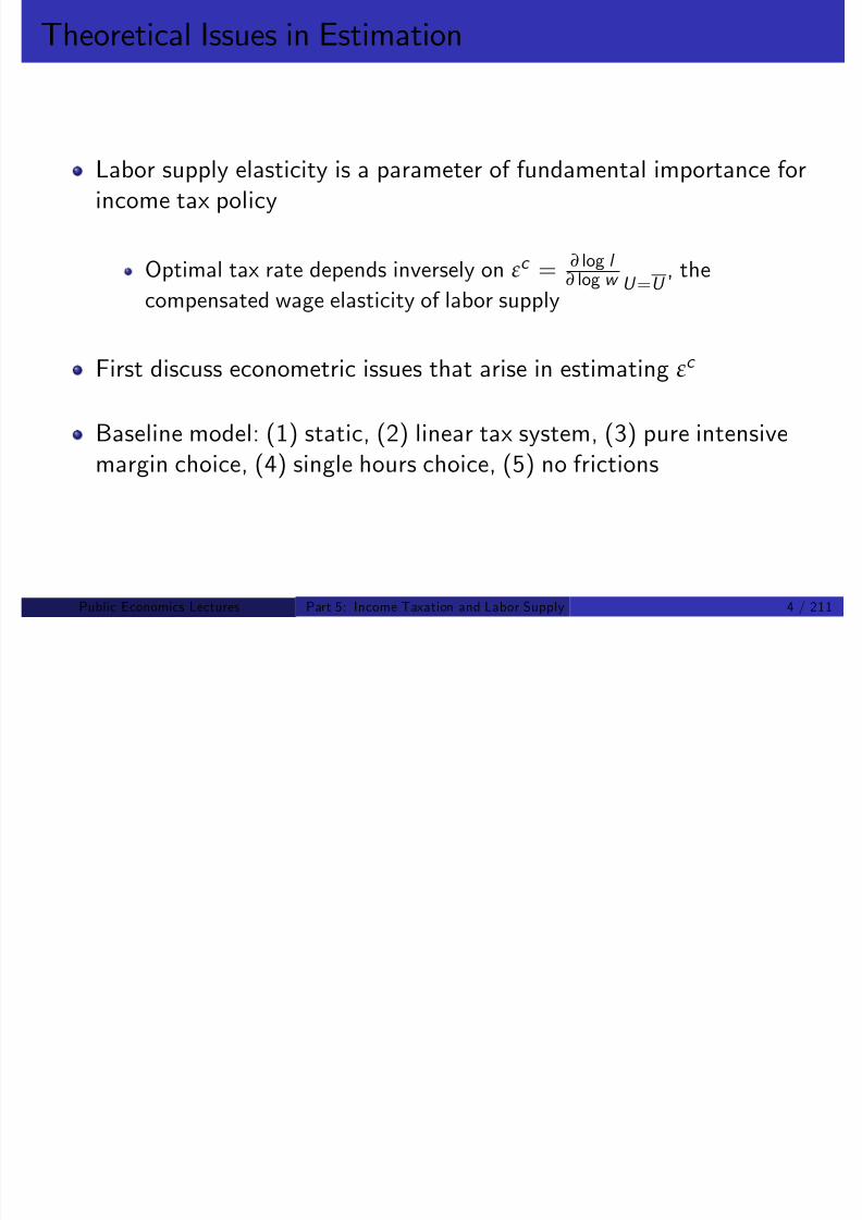
8/8/2019 Chetty - Public Economics Lectures
http://slidepdf.com/reader/full/chetty-public-economics-lectures 399/949
Baseline Labor-Leisure Choice Model: Key Assumptions
1 Static model
2 Intensive-margin, one dimensional choice
3 No frictions or adjustment costs
4 Linear tax system
Public Economics Lectures ()Part 5: Income Taxation and Labor Supply 5 / 211

8/8/2019 Chetty - Public Economics Lectures
http://slidepdf.com/reader/full/chetty-public-economics-lectures 400/949
Static Model: Setup
Let c denote consumption and l hours worked
Normalize price of c to one
Agent has utility u (c , l ) = c al 1+1/ε
1+1/ε
Agent earns wage w per hour worked and has y in non-labor income
With tax rate τ on labor income, Individual solves
max u (c , l ) s.t. c = (1 τ )wl + y
Public Economics Lectures ()Part 5: Income Taxation and Labor Supply 6 / 211

8/8/2019 Chetty - Public Economics Lectures
http://slidepdf.com/reader/full/chetty-public-economics-lectures 401/949

8/8/2019 Chetty - Public Economics Lectures
http://slidepdf.com/reader/full/chetty-public-economics-lectures 402/949
Problems with OLS Estimation of Labor Supply Equation
1 Econometric issuesUnobserved heterogeneity [tax instruments]
Measurement error in wages and division bias [tax instruments]
Selection into labor force [panel data]
2 Extensive vs. intensive margin responses [participation models]
3 Non-hours responses [taxable income]
4 Incorporating progressive taxes [non-linear budget set methods]
Public Economics Lectures ()Part 5: Income Taxation and Labor Supply 8 / 211

8/8/2019 Chetty - Public Economics Lectures
http://slidepdf.com/reader/full/chetty-public-economics-lectures 403/949
Econometric Problem 1: Unobserved Heterogeneity
Early studies estimated elasticity using cross-sectional variation inwage rates
Problem: unobserved heterogeneity
Those with high wages also have a high propensity to work
Cross-sectional correlation between w and h likely to yield an upwardbiased estimate of ε
Solution: use taxes as instruments for (1 τ )w
Public Economics Lectures ()Part 5: Income Taxation and Labor Supply 9 / 211
8/8/2019 Chetty - Public Economics Lectures
http://slidepdf.com/reader/full/chetty-public-economics-lectures 404/949
Econometric Problem 2: Measurement Error/Division Bias
Wage w is typically not observed; backed out from dividing earningsby reported hours
When hours are measured with noise, this can lead to “division bias”
Let l denote true hours, l observed hours
Compute w = e l
where e is earnings
) log l = log l + µ
) log w = log e log l = log e log l µ = log w µ
Public Economics Lectures ()Part 5: Income Taxation and Labor Supply 10 / 211

8/8/2019 Chetty - Public Economics Lectures
http://slidepdf.com/reader/full/chetty-public-economics-lectures 405/949
Measurement Error and Division Bias
Mis-measurement of hours causes a spurious link between hours andwages
Estimate a regression of the following form:
log l = β1 + β2 log w + ε
Then
E b β2 =cov (log l , log w )
var (log w )=
cov (log l + µ, log w µ)
var (log w ) + var (µ)
Problem: E b β2
6= ε because orthogonality restriction for OLS violated
Ex. workers with high mis-reported hours also have low imputedwages, biasing elasticity estimate downward
Solution: tax instruments again
Public Economics Lectures ()Part 5: Income Taxation and Labor Supply 11 / 211

8/8/2019 Chetty - Public Economics Lectures
http://slidepdf.com/reader/full/chetty-public-economics-lectures 406/949
Econometric Problem 3: Selection into Labor Force
Consider model with …xed costs of working, where some individualschoose not to work
Wages are unobserved for non-labor force participants
Thus, OLS regression on workers only includes observations withl i > 0
This can bias OLS estimates: low wage earners must have very highunobserved propensity to work to …nd it worthwhile
Requires a selection correction (e.g. Heckit, Tobit, or ML estimation)
See Killingsworth and Heckman (1986) for implementation
Current approach: use panel data to distinguish entry/exit fromintensive-margin changes
Public Economics Lectures ()Part 5: Income Taxation and Labor Supply 12 / 211

8/8/2019 Chetty - Public Economics Lectures
http://slidepdf.com/reader/full/chetty-public-economics-lectures 407/949
Extensive vs. Intensive Margin
Related issue: want to understand e¤ect of taxes on labor force
participation decision
With …xed costs of work, individuals may jump from non-participationto part time or full time work (non-convex budget set)
This can be handled using a discrete choice model:
P = φ(α + ε log(1 τ ) ηy )
where P 2 f0, 1g is an indicator for whether the individual works
Function φ typically speci…ed as logit, probit, or linear prob model
Note: here it is critical to have tax variation; regression cannot be runwith wage variation
Public Economics Lectures ()Part 5: Income Taxation and Labor Supply 13 / 211

8/8/2019 Chetty - Public Economics Lectures
http://slidepdf.com/reader/full/chetty-public-economics-lectures 408/949
Non-Hours Responses
Traditional literature focused purely on hours of work and labor force
participation
Problem: income taxes distort many margins beyond hours of work
More important responses may be on those margins
Hours very hard to measure (most ppl report 40 hours per week)
Two solutions in modern literature:
Focus on taxable income (wl ) as a broader measure of labor supply(Feldstein 1995)
Focus on subgroups of workers for whom hours are better measured,e.g. taxi drivers
Public Economics Lectures ()Part 5: Income Taxation and Labor Supply 14 / 211

8/8/2019 Chetty - Public Economics Lectures
http://slidepdf.com/reader/full/chetty-public-economics-lectures 409/949
Progressive Taxes and Labor Supply
OLS regression speci…cation is derived from model with a single lineartax rate
In practice, income tax systems are non-linear
Consider e¤ect of US income tax code on budget sets
Public Economics Lectures ()Part 5: Income Taxation and Labor Supply 15 / 211

8/8/2019 Chetty - Public Economics Lectures
http://slidepdf.com/reader/full/chetty-public-economics-lectures 410/949
Source: Congressional Budget O¢ce 2005
Public Economics Lectures ()Part 5: Income Taxation and Labor Supply 16 / 211
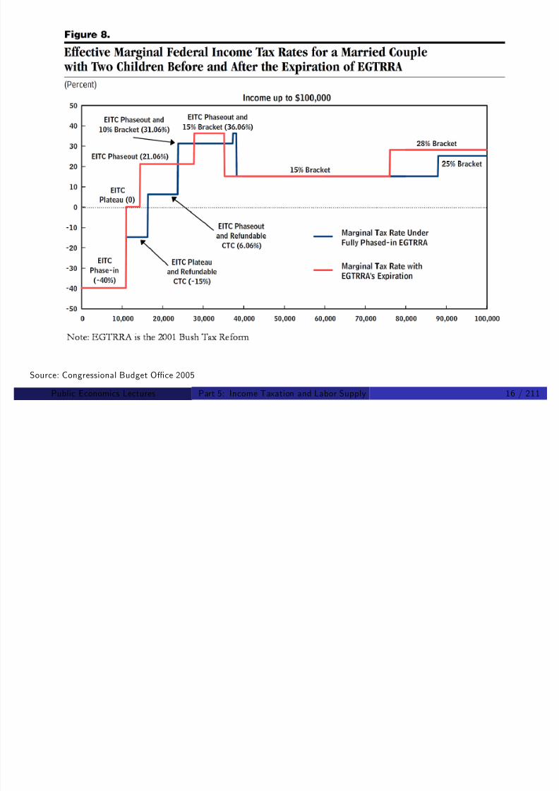
8/8/2019 Chetty - Public Economics Lectures
http://slidepdf.com/reader/full/chetty-public-economics-lectures 411/949
Example 1: Progressive Income Tax
Public Economics Lectures ()Part 5: Income Taxation and Labor Supply 17 / 211
E l 2 EITC
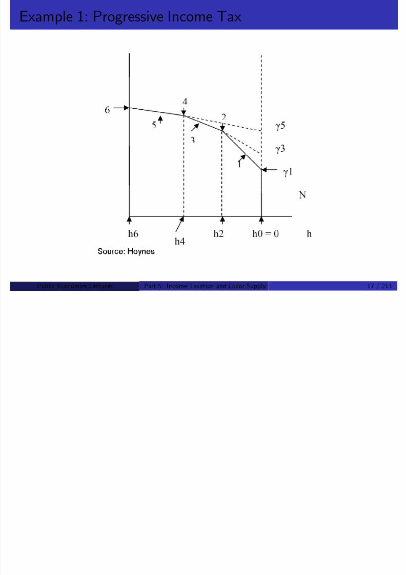
8/8/2019 Chetty - Public Economics Lectures
http://slidepdf.com/reader/full/chetty-public-economics-lectures 412/949
Example 2: EITC
Public Economics Lectures ()Part 5: Income Taxation and Labor Supply 18 / 211
E l 3 S i l S i P ll T C

8/8/2019 Chetty - Public Economics Lectures
http://slidepdf.com/reader/full/chetty-public-economics-lectures 413/949
Example 3: Social Security Payroll Tax Cap
Public Economics Lectures ()Part 5: Income Taxation and Labor Supply 19 / 211
E l 4 N i I T

8/8/2019 Chetty - Public Economics Lectures
http://slidepdf.com/reader/full/chetty-public-economics-lectures 414/949
Example 4: Negative Income Tax
Public Economics Lectures ()Part 5: Income Taxation and Labor Supply 20 / 211
P i T d L b S l
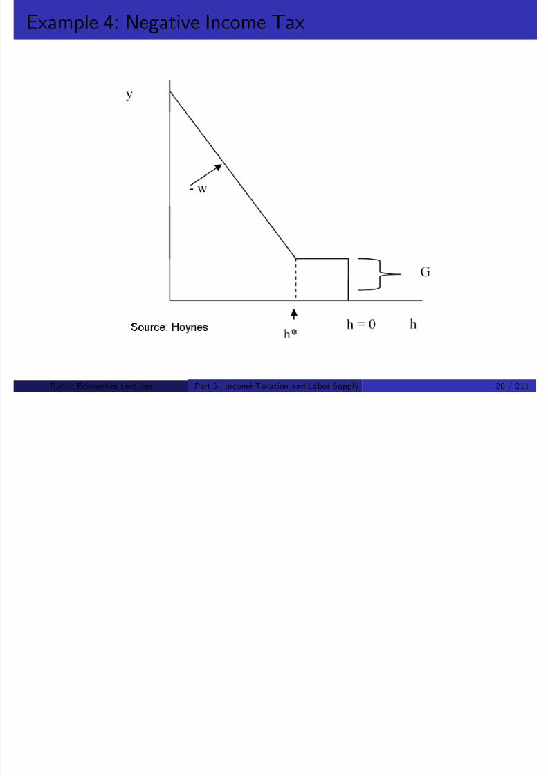
8/8/2019 Chetty - Public Economics Lectures
http://slidepdf.com/reader/full/chetty-public-economics-lectures 415/949
Progressive Taxes and Labor Supply
Non-linear budget set creates two problems:
1 Model mis-speci…cation: OLS regression no longer recovers structuralelasticity parameter ε of interest
Two reasons: (1) underestimate response because people pile up atkink and (2) mis-estimate income e¤ects
2 Econometric bias: τ i depends on income w i l i and hence on l i
Tastes for work are positively correlated with τ i ! downward bias in
OLS regression of hours worked on net-of-tax rates
Solution to problem #2: only use reform-based variation in tax rates
But problem #1 requires fundamentally di¤erent estimation method
Public Economics Lectures ()Part 5: Income Taxation and Labor Supply 21 / 211
H N li B d t C t i t

8/8/2019 Chetty - Public Economics Lectures
http://slidepdf.com/reader/full/chetty-public-economics-lectures 416/949
Hausman: Non-linear Budget Constraints
Hausman pioneered structural approach to estimating elasticities withnon-linear budget sets
Assume an uncompensated labor supply equation:
l = α + βw (1 τ ) + γy +
Error term is normally distributed with variance σ 2
Observed variables: w i , τ i , y i , and l i
Technique: (1) construct likelihood function given observed labor
supply choices on NLBS, (2) …nd parameters (α, β, γ) that maximizelikelihood
Important insight: need to use “virtual incomes” in lieu of actualunearned income with NLBS
Public Economics Lectures ()Part 5: Income Taxation and Labor Supply 22 / 211
8/8/2019 Chetty - Public Economics Lectures
http://slidepdf.com/reader/full/chetty-public-economics-lectures 417/949
Non-Linear Budget Set Estimation: Virtual Incomes
Source: Hausman 1985
L1L2 l*-L
$
y1
y2
y3
w3
w2
w1
Public Economics Lectures ()Part 5: Income Taxation and Labor Supply 23 / 211
NLBS Likelihood Function

8/8/2019 Chetty - Public Economics Lectures
http://slidepdf.com/reader/full/chetty-public-economics-lectures 418/949
NLBS Likelihood Function
Consider a two-bracket tax system
Individual can locate on …rst bracket, on second bracket, or at thekink l K
Likelihood = probability that we see individual i at labor supply l i given a parameter vector
Decompose likelihood into three components
Component 1: individual i on …rst bracket: 0 < l i < l K
l i = α + βw i (1 τ 1) + γy 1 + i
Error i = l i (α + βw i (1 τ 1) + γy 1). Likelihood:Li = φ((l i (α + βw i (1 τ 1) + γy 1)/σ )
Component 2: individual i on second bracket: l K < l i . Likelihood:
Li = φ((l i (α + βw i (1 τ 2) + γy 2)/σ )
Public Economics Lectures ()Part 5: Income Taxation and Labor Supply 24 / 211
Likelihood Function: Located at the Kink

8/8/2019 Chetty - Public Economics Lectures
http://slidepdf.com/reader/full/chetty-public-economics-lectures 419/949
Likelihood Function: Located at the Kink
Now consider individual i located at the kink point
If tax rate is τ 1 and virtual income y 1 individual wants to work l > l K
If tax is τ 2 and virtual income y 2 individual wants to work l < l K
These inequalities imply:
α + βw i (1 τ 1) + γy 1 + i > l K > α + βw i (1 τ 2) + γy 2 + i
l K (α + βw i (1 τ 1) + γy 1) < i < l K (α + βw i (1 τ 2) + γy 2
Contribution to likelihood is probability that error lies in this range:
Li = Ψ[(l K (α + βw i (1 τ 2) + γy 2))/σ ]
Ψ[(l K (α + βw i (1 τ 1) + γy 1))/σ ]
Public Economics Lectures ()Part 5: Income Taxation and Labor Supply 25 / 211
Maximum Likelihood Estimation

8/8/2019 Chetty - Public Economics Lectures
http://slidepdf.com/reader/full/chetty-public-economics-lectures 420/949
Maximum Likelihood Estimation
Log likelihood function is L = ∑ i log Li
Final step is solving
max L(α, β, γ, σ )In practice, likelihood function much more complicated because of more kinks, non-convexities, and covariates
But basic technique remains the same
Public Economics Lectures ()Part 5: Income Taxation and Labor Supply 26 / 211
Hausman (1981) Application
8/8/2019 Chetty - Public Economics Lectures
http://slidepdf.com/reader/full/chetty-public-economics-lectures 421/949
Hausman (1981) Application
Hausman applies method to 1975 PSID cross-section
Finds signi…cant compensated elasticities and large income e¤ects
Elasticities larger for women than for men
Shortcomings of this implementation
1 Sensitivity to functional form choices, which is a larger issue withstructural estimation
2 No tax reforms, so does not solve fundamental econometric problemthat tastes for work may be correlated with w
Public Economics Lectures ()Part 5: Income Taxation and Labor Supply 27 / 211
NLBS and Bunching at Kinks

8/8/2019 Chetty - Public Economics Lectures
http://slidepdf.com/reader/full/chetty-public-economics-lectures 422/949
NLBS and Bunching at Kinks
Subsequent studies obtain di¤erent estimates (MaCurdy, Green, andPaarsh 1990, Blomquist 1995)
Several studies …nd negative compensated wage elasticity estimates
Debate: impose requirement that compensated elasticity is positive or
conclude that data rejects model?
Fundamental source of problem: labor supply model predicts thatindividuals should bunch at the kink points of the tax schedule
But we observe very little bunching at kinks, so model is rejected bythe data
Interest in NLBS models diminished despite their conceptualadvantages over OLS methods
Public Economics Lectures ()Part 5: Income Taxation and Labor Supply 28 / 211
Saez 2009: Bunching at Kinks

8/8/2019 Chetty - Public Economics Lectures
http://slidepdf.com/reader/full/chetty-public-economics-lectures 423/949
Saez 2009: Bunching at Kinks
Saez observes that only non-parametric source of identi…cation forelasticity in a cross-section is amount of bunching at kinks
All other tax variation is contaminated by heterogeneity in tastes
Develops method of using bunching at kinks to estimate the
compensated taxable income elasticity
Idea: if this simple, non-parametric method does not recover positivecompensated elasticities, then little value in additional structure of NLBS models
Formula for elasticity:
εc =dz /z
dt /(1 t )=
excess mass at kink
% change in NTR
Public Economics Lectures ()Part 5: Income Taxation and Labor Supply 29 / 211
8/8/2019 Chetty - Public Economics Lectures
http://slidepdf.com/reader/full/chetty-public-economics-lectures 424/949
Public Economics Lectures ()Part 5: Income Taxation and Labor Supply 30 / 211

8/8/2019 Chetty - Public Economics Lectures
http://slidepdf.com/reader/full/chetty-public-economics-lectures 425/949
Public Economics Lectures ()Part 5: Income Taxation and Labor Supply 31 / 211
Saez 2009: Bunching at Kinks

8/8/2019 Chetty - Public Economics Lectures
http://slidepdf.com/reader/full/chetty-public-economics-lectures 426/949
Saez 2009: Bunching at Kinks
Saez implements this method using individual tax return micro data
(IRS public use …les) from 1960 to 2004
Advantage of dataset over PSID: very little measurement error
Finds bunching around:
First kink point of the Earned Income Tax Credit, especially forself-employed
At threshold of the …rst tax bracket where tax liability starts, especiallyin the 1960s when this point was very stable
However, no bunching observed around all other kink points
Public Economics Lectures ()Part 5: Income Taxation and Labor Supply 32 / 211
Earnings Density and the EITC: Wage Earners vs. Self-Employed

8/8/2019 Chetty - Public Economics Lectures
http://slidepdf.com/reader/full/chetty-public-economics-lectures 427/949
g y g p y
Public Economics Lectures ()Part 5: Income Taxation and Labor Supply 33 / 211
Earnings Density and the EITC: Wage Earners vs. Self-Employed

8/8/2019 Chetty - Public Economics Lectures
http://slidepdf.com/reader/full/chetty-public-economics-lectures 428/949
g y g p y
Public Economics Lectures ()Part 5: Income Taxation and Labor Supply 34 / 211
Taxable Income Density 1960-1969: Bunching around First Kink

8/8/2019 Chetty - Public Economics Lectures
http://slidepdf.com/reader/full/chetty-public-economics-lectures 429/949
Taxable Income Density, 1960 1969: Bunching around First Kink
Public Economics Lectures ()Part 5: Income Taxation and Labor Supply 35 / 211
Taxable Income Density, 1960-1969: Bunching around First Kink

8/8/2019 Chetty - Public Economics Lectures
http://slidepdf.com/reader/full/chetty-public-economics-lectures 430/949
Taxable Income Density, 1960 1969: Bunching around First Kink
Public Economics Lectures ()Part 5: Income Taxation and Labor Supply 36 / 211
Friedberg 2000: Social Security Earnings Test

8/8/2019 Chetty - Public Economics Lectures
http://slidepdf.com/reader/full/chetty-public-economics-lectures 431/949
Uses CPS data on labor supply of retirees receiving Social Securitybene…ts
Studies bunching based on responses to Social Security earnings test
Earnings test: phaseout of SS bene…ts above an exempt amount
Phaseout rate varies by age group - 50%, 33%, 0 (lower for older
workers)
Public Economics Lectures ()Part 5: Income Taxation and Labor Supply 37 / 211

8/8/2019 Chetty - Public Economics Lectures
http://slidepdf.com/reader/full/chetty-public-economics-lectures 432/949
Public Economics Lectures ()Part 5: Income Taxation and Labor Supply 38 / 211
Friedberg: Estimates

8/8/2019 Chetty - Public Economics Lectures
http://slidepdf.com/reader/full/chetty-public-economics-lectures 433/949
Estimates elasticities using Hausman method, …nds relatively largecompensated and uncompensated elasticities
Ironically, lost social security bene…ts are considered delayedretirement with an actuarial adjustment of future bene…ts
!So the one kink where we do …nd real bunching is actually not real!
Public Economics Lectures ()Part 5: Income Taxation and Labor Supply 39 / 211
Borenstein 2009: Electricity Consumption

8/8/2019 Chetty - Public Economics Lectures
http://slidepdf.com/reader/full/chetty-public-economics-lectures 434/949
Public Economics Lectures ()Part 5: Income Taxation and Labor Supply 40 / 211

8/8/2019 Chetty - Public Economics Lectures
http://slidepdf.com/reader/full/chetty-public-economics-lectures 435/949
Public Economics Lectures ()Part 5: Income Taxation and Labor Supply 41 / 211
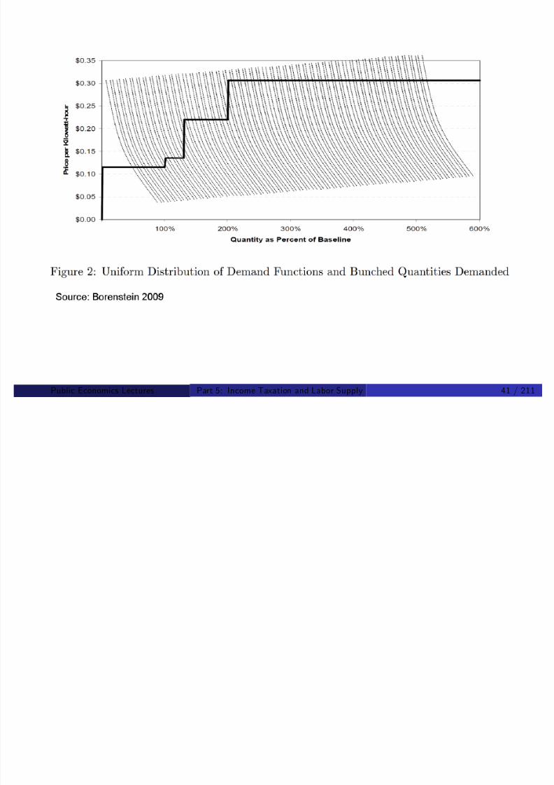
8/8/2019 Chetty - Public Economics Lectures
http://slidepdf.com/reader/full/chetty-public-economics-lectures 436/949
Public Economics Lectures ()Part 5: Income Taxation and Labor Supply 42 / 211
Why not more bunching at kinks?
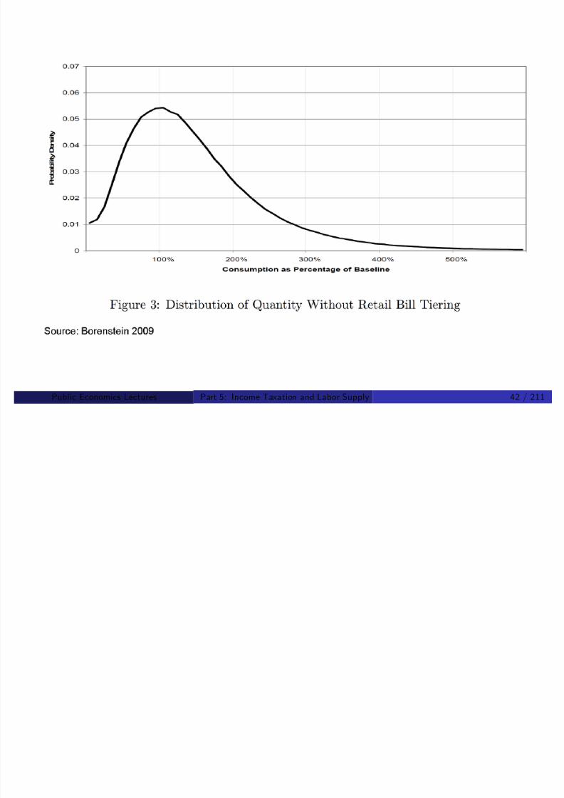
8/8/2019 Chetty - Public Economics Lectures
http://slidepdf.com/reader/full/chetty-public-economics-lectures 437/949
1
True elasticity of response may be small
2 Randomness in income generation process
3 Information and salience
Liebman and Zeckhauser: “Schmeduling”
Chetty and Saez (2009): information signi…cantly a¤ects bunching inEITC …eld experiment
4 Adjustment costs and institutional constraints (Chetty et al 2009)
Public Economics Lectures ()Part 5: Income Taxation and Labor Supply 43 / 211
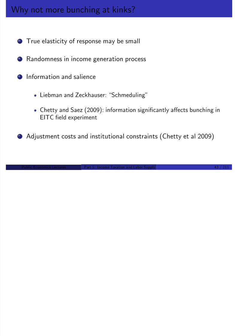
8/8/2019 Chetty - Public Economics Lectures
http://slidepdf.com/reader/full/chetty-public-economics-lectures 438/949
Public Economics Lectures ()Part 5: Income Taxation and Labor Supply 44 / 211

8/8/2019 Chetty - Public Economics Lectures
http://slidepdf.com/reader/full/chetty-public-economics-lectures 439/949
Public Economics Lectures ()Part 5: Income Taxation and Labor Supply 45 / 211
Chetty, Friedman, Olsen, and Pistaferri (2009)

8/8/2019 Chetty - Public Economics Lectures
http://slidepdf.com/reader/full/chetty-public-economics-lectures 440/949
If workers face adjustment costs, may not reoptimize in response totax changes of small size and scope in short run
Search costs, costs of acquiring information about taxes
Institutional constraints imposed by …rms (e.g. 40 hour week)
Could explain why macro studies …nd larger elasticities
Question: How much are elasticity estimates a¤ected by frictions?
Public Economics Lectures ()Part 5: Income Taxation and Labor Supply 46 / 211
Chetty et al. 2009: Model

8/8/2019 Chetty - Public Economics Lectures
http://slidepdf.com/reader/full/chetty-public-economics-lectures 441/949
Firms post jobs with di¤erent hours o¤ers
Workers draw from this distribution and must pay search cost to
reoptimize
Therefore not all workers locate at optimal choice
Bunching at kink and observed responses to tax reforms attenuated
Public Economics Lectures ()Part 5: Income Taxation and Labor Supply 47 / 211
Chetty et al. 2009: Testable Predictions

8/8/2019 Chetty - Public Economics Lectures
http://slidepdf.com/reader/full/chetty-public-economics-lectures 442/949
Model generates three predictions:
1 [Size] Larger tax changes generate larger observed elasticities
Large tax changes are more likely to induce workers to search for adi¤erent job
2 [Scope] Tax changes that apply to a larger group of workers generatelarger observed elasticities
Firms tailor jobs to preferences of common workers
3 [Search Costs] Workers with lower search costs exhibit largerelasticities from individual bunching
Public Economics Lectures ()Part 5: Income Taxation and Labor Supply 48 / 211
Cost of Bunching at Bracket Cuto¤ Points in Tax Schedule
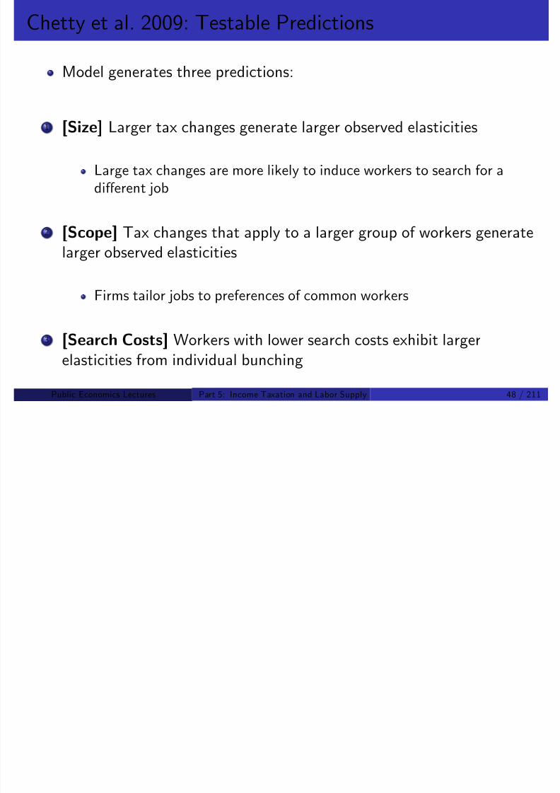
8/8/2019 Chetty - Public Economics Lectures
http://slidepdf.com/reader/full/chetty-public-economics-lectures 443/949
Hours Worked (h)
C o n s u m p t i o n ( c )
h*h h_h_
_
U(c,h) = U*
U(c,h) = U* – φ
_h’
Slope = (1 – τ2)w
Slope =
Slope = (1 – τ2’)w
(1 – τ1)w
Source: Chetty et al. 2009
Public Economics Lectures ()Part 5: Income Taxation and Labor Supply 49 / 211
Chetty et al. 2009: Data

8/8/2019 Chetty - Public Economics Lectures
http://slidepdf.com/reader/full/chetty-public-economics-lectures 444/949
Matched employer-employee panel data with admin tax records forfull population of Denmark
Income vars: wage earnings, capital and stock income, pensioncontributions
Employer vars: tenure, occupation, employer ID
Demographics: education, spouse ID, kids, municipality
Sample restriction: Wage-earners aged 15-70, 1994-2001
Approximately 2.42 million people per year
Public Economics Lectures ()Part 5: Income Taxation and Labor Supply 50 / 211
Marginal Tax Rates in Denmark in 2000

8/8/2019 Chetty - Public Economics Lectures
http://slidepdf.com/reader/full/chetty-public-economics-lectures 445/949
6 0
0
2 0
4 0
8 0
100 200 300 40050 150150 250 350
Taxable Income (1000s DKR)
M a r g i n a l T a x R a t e ( % )
∆log(NTR) = -11%
∆log(NTR) = -33%
Note: $1 ≅ 6 DKr
Source: Chetty et al. 2009
Public Economics Lectures ()Part 5: Income Taxation and Labor Supply 51 / 211
Income Distribution for Wage Earners Around Top Tax Cutoff

8/8/2019 Chetty - Public Economics Lectures
http://slidepdf.com/reader/full/chetty-public-economics-lectures 446/949
2 0 0 0 0
4 0 0 0 0
6 0 0 0 0
8 0 0 0 0
1 0 0 0 0 0
-50 -40 -30 -20 -10 0 10 20 30 40 50
Taxable Income Relative to Top Bracket Cutoff (1000s DKr)
F r e q u e n c y
Source: Chetty et al. 2009
Public Economics Lectures ()Part 5: Income Taxation and Labor Supply 52 / 211
Income Distribution for Wage Earners Around Top Tax Cutoff

8/8/2019 Chetty - Public Economics Lectures
http://slidepdf.com/reader/full/chetty-public-economics-lectures 447/949
2 0 0 0 0
4 0 0 0 0
6 0 0 0 0
8 0 0 0 0
1 0 0 0 0 0
-50 -40 -30 -20 -10 0 10 20 30 40 50
Taxable Income Relative to Top Bracket Cutoff (1000s DKr)
F r e q u e n c y
Source: Chetty et al. 2009
Excess mass = BÝAbÞ
Public Economics Lectures ()Part 5: Income Taxation and Labor Supply 53 / 211
Income Distribution for Wage Earners Around Top Tax Cutoff

8/8/2019 Chetty - Public Economics Lectures
http://slidepdf.com/reader/full/chetty-public-economics-lectures 448/949
2 0 0 0 0
4 0 0 0 0
6 0 0 0 0
8 0 0 0 0
1 0 0 0 0 0
-50 -40 -30 -20 -10 0 10 20 30 40 50
Taxable Income Relative to Top Bracket Cutoff (1000s DKr)
F r e q u e n c y
Excess mass (b ) = 0.81
Standard error = 0.05
Source: Chetty et al. 2009
Public Economics Lectures ()Part 5: Income Taxation and Labor Supply 54 / 211
Married Women vs. Single MenMarried Women vs. Single Men

8/8/2019 Chetty - Public Economics Lectures
http://slidepdf.com/reader/full/chetty-public-economics-lectures 449/949
1 0 0 0 0
2
0 0 0 0
3 0 0
0 0
1 0 0 0 0
2 0 0 0 0
3 0 0 0 0
-50 -40 -30 -20 -10 0 10 20 30 40 50
0
F r e q u e n c
y ( m a r r i e d w o m e n )
F r e q u e
n c y ( s i n g l e m e n )
Taxable Income Relative to Top Bracket Cutoff (1000s DKr)
Married Women
Excess mass (b )= 1.79Standard error = 0.10
Single Men
Excess mass (b ) = 0.25Standard error = 0.04
1 0 0 0 0
2
0 0 0 0
3 0 0
0 0
1 0 0 0 0
2 0 0 0 0
3 0 0 0 0
-50 -40 -30 -20 -10 0 10 20 30 40 50
0
F r e q u e n c
y ( m a r r i e d w o m e n )
F r e q u e
n c y ( s i n g l e m e n )
Taxable Income Relative to Top Bracket Cutoff (1000s DKr)
Married Women
Excess mass (b )= 1.79Standard error = 0.10
Single Men
Excess mass (b ) = 0.25Standard error = 0.04
Source: Chetty et al. 2009
Public Economics Lectures ()Part 5: Income Taxation and Labor Supply 55 / 211
0 0
Teachers vs. Military
0 0
Teachers vs. Military
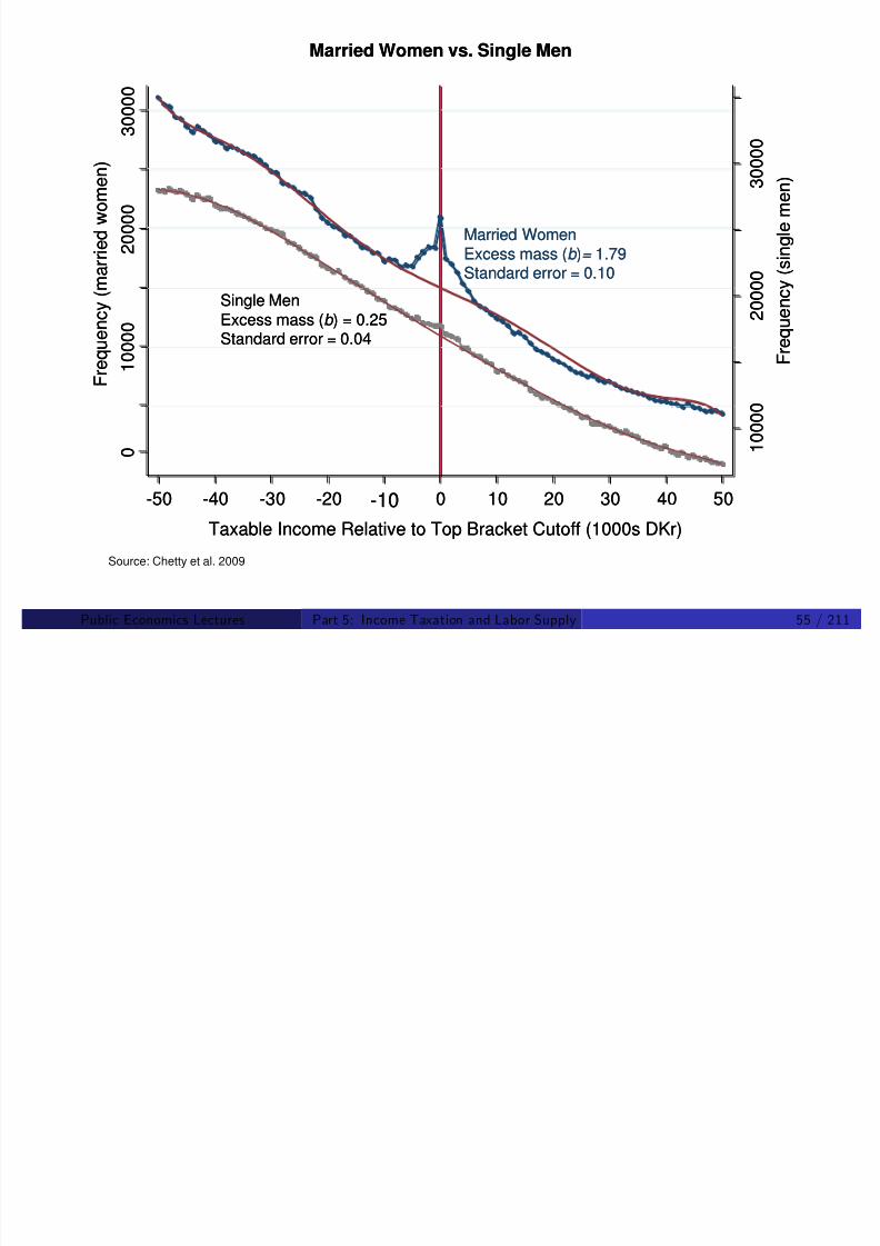
8/8/2019 Chetty - Public Economics Lectures
http://slidepdf.com/reader/full/chetty-public-economics-lectures 450/949
0
1 0 0 0
2 0 0 0
3 0 0 0
4 0 0
0
2 0 0 0
4 0 0 0
6 0 0 0
8 0 0 0
-50 -40 -30 -20 -10 0 10 20 30 40 50
F r e q u
e n c y ( t e a c h e r s )
F r e q u e n c y ( m i l i t a r y )
Taxable Income Relative to Top Bracket Cutoff (1000s DKr)
TeachersExcess mass (b )= 3.54Standard error = 0.25
MilitaryExcess mass (b ) = -0.12Standard error = 0.21
0
1 0 0 0
2 0 0 0
3 0 0 0
4 0 0
0
2 0 0 0
4 0 0 0
6 0 0 0
8 0 0 0
-50 -40 -30 -20 -10 0 10 20 30 40 50
F r e q u
e n c y ( t e a c h e r s )
F r e q u e n c y ( m i l i t a r y )
Taxable Income Relative to Top Bracket Cutoff (1000s DKr)
TeachersExcess mass (b )= 3.54Standard error = 0.25
MilitaryExcess mass (b ) = -0.12Standard error = 0.21
Source: Chetty et al. 2009
Public Economics Lectures ()Part 5: Income Taxation and Labor Supply 56 / 211
0
Taxable Income Distributions in 1994
0
Taxable Income Distributions in 1994

8/8/2019 Chetty - Public Economics Lectures
http://slidepdf.com/reader/full/chetty-public-economics-lectures 451/949
F r e q u e n c
y ( a l l w a g e e a r n e r s )
F r e q u e n
c y ( m a r r i e d w o m e
n )
0
1 0 0 0
2 0 0 0
3 0 0 0
4 0 0 0
6 0 0 0
8 0 0 0
1 0 0 0 0 1 2 0 0 0
1 4 0 0 0
210 220 230 240 250 260 270 280 290 300Taxable Income (1000s DKR)
All Wage EarnersExcess Mass (b) = 0.61Standard error = 0.08
Married WomenExcess Mass (b) = 1.03Standard error = 0.14
Source: Chetty et al. 2009
Public Economics Lectures ()Part 5: Income Taxation and Labor Supply 57 / 211
0 0
1995
0 0
1995

8/8/2019 Chetty - Public Economics Lectures
http://slidepdf.com/reader/full/chetty-public-economics-lectures 452/949
1 0 0 0
2 0 0 0
3 0 0
0
4 0 0 0
8 0 0 0
1 2 0 0
0
210 220 230 240 250 260 270 280 290 300
Taxable Income (1000s DKR)
b = 1.25s.e. = 0.16
b = 0.41s.e. = 0.08
F r e q u e n c
y ( a l l w a g e e a r n e r s )
F r e q u e n
c y ( m a r r i e d w o m e
n )
1 0 0 0
2 0 0 0
3 0 0
0
4 0 0 0
8 0 0 0
1 2 0 0
0
210 220 230 240 250 260 270 280 290 300
Taxable Income (1000s DKR)
b = 1.25s.e. = 0.16
b = 0.41s.e. = 0.08
F r e q u e n c
y ( a l l w a g e e a r n e r s )
F r e q u e n
c y ( m a r r i e d w o m e
n )
Source: Chetty et al. 2009
Public Economics Lectures ()Part 5: Income Taxation and Labor Supply 58 / 211
19961996

8/8/2019 Chetty - Public Economics Lectures
http://slidepdf.com/reader/full/chetty-public-economics-lectures 453/949
1 0 0 0
2 0 0 0
3 0 0 0
0 4 0 0 0
8 0
0 0
1 2 0 0 0
210 220 230 240 250 260 270 280 290 300
Taxable Income (1000s DKR)
F r e q u e n c
y ( a l l w a g e e a r n e r
s )
F r e q u e n c y ( m a r r i e d w o m e
n )
b = 1.55s.e. = 0.17
b = 0.66
s.e. = 0.09
1 0 0 0
2 0 0 0
3 0 0 0
0 4 0 0 0
8 0
0 0
1 2 0 0 0
210 220 230 240 250 260 270 280 290 300
Taxable Income (1000s DKR)
F r e q u e n c
y ( a l l w a g e e a r n e r
s )
F r e q u e n c y ( m a r r i e d w o m e
n )
b = 1.55s.e. = 0.17
b = 0.66
s.e. = 0.09
Source: Chetty et al. 2009
Public Economics Lectures ()Part 5: Income Taxation and Labor Supply 59 / 211
19971997
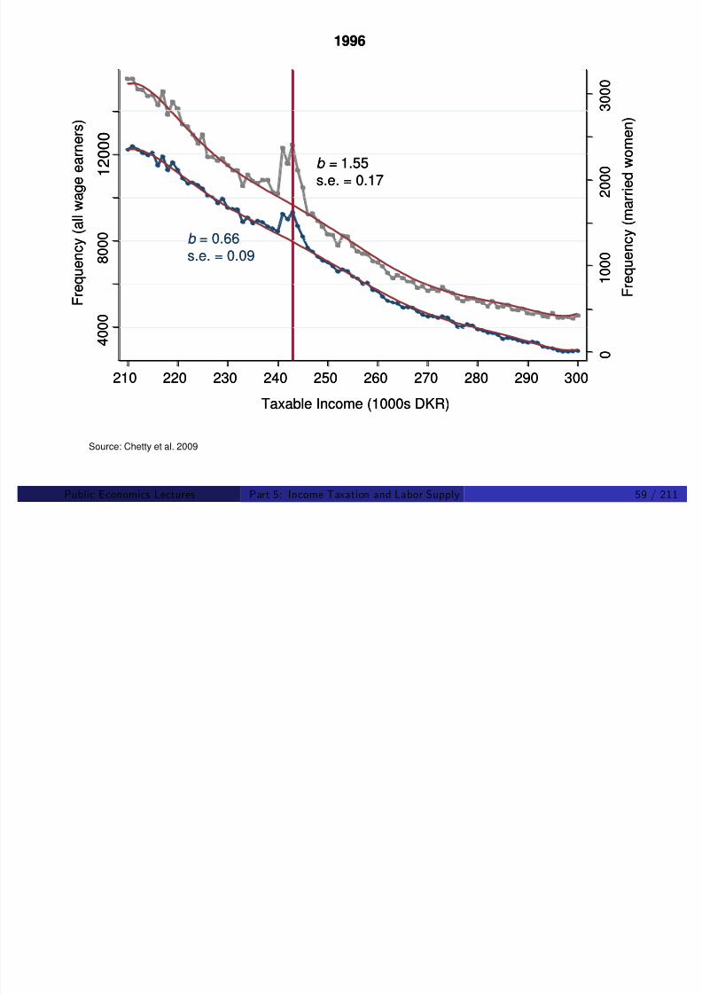
8/8/2019 Chetty - Public Economics Lectures
http://slidepdf.com/reader/full/chetty-public-economics-lectures 454/949
0
1 0 0 0
2 0 0 0
3 0 0 0
5 0 0 0
1 0 0 0 0
1
5 0 0 0
210 220 230 240 250 260 270 280 290 300
Taxable Income (1000s DKR)
F r e q u e n c
y ( a l l w a g e e a r n e r s )
F r e q u e n
c y ( m a r r i e d w o m e
n )
b = 1.26s.e. = 0.19
b = 0.58
s.e. = 0.01
0
1 0 0 0
2 0 0 0
3 0 0 0
5 0 0 0
1 0 0 0 0
1
5 0 0 0
210 220 230 240 250 260 270 280 290 300
Taxable Income (1000s DKR)
F r e q u e n c
y ( a l l w a g e e a r n e r s )
F r e q u e n
c y ( m a r r i e d w o m e
n )
b = 1.26s.e. = 0.19
b = 0.58
s.e. = 0.01
Source: Chetty et al. 2009
Public Economics Lectures ()Part 5: Income Taxation and Labor Supply 60 / 211
19981998

8/8/2019 Chetty - Public Economics Lectures
http://slidepdf.com/reader/full/chetty-public-economics-lectures 455/949
0
1 0 0 0
2 0 0 0
3 0 0 0
4 0 0 0
8 0 0 0
1 2 0 0 0
210 220 230 240 250 260 270 280 290 300
Taxable Income (1000s DKR)
F r e q u e n c
y ( a l l w a g e e a r n e r s )
F r e q u e n
c y ( m a r r i e d w o m e
n )
b = 1.71s.e. = 0.18
b = 0.78
s.e. = 0.09
0
1 0 0 0
2 0 0 0
3 0 0 0
4 0 0 0
8 0 0 0
1 2 0 0 0
210 220 230 240 250 260 270 280 290 300
Taxable Income (1000s DKR)
F r e q u e n c
y ( a l l w a g e e a r n e r s )
F r e q u e n
c y ( m a r r i e d w o m e
n )
b = 1.71s.e. = 0.18
b = 0.78
s.e. = 0.09
Source: Chetty et al. 2009
Public Economics Lectures ()Part 5: Income Taxation and Labor Supply 61 / 211
0 0 0
1999
0 0 0
1999

8/8/2019 Chetty - Public Economics Lectures
http://slidepdf.com/reader/full/chetty-public-economics-lectures 456/949
0
1 0 0 0
2 0 0 0
3 0 0 0
4 0
4 0
0 0
8 0 0 0
1 2 0 0 0
210 220 230 240 250 260 270 280 290 300
Taxable Income (1000s DKR)
F r e q u e n c
y ( a l l w a g e e a r n e r
s )
F r e q u e n c y ( m a r r i e d w o m e
n )
b = 1.49s.e. = 0.16
b = 0.62
s.e. = 0.08
0
1 0 0 0
2 0 0 0
3 0 0 0
4 0
4 0
0 0
8 0 0 0
1 2 0 0 0
210 220 230 240 250 260 270 280 290 300
Taxable Income (1000s DKR)
F r e q u e n c
y ( a l l w a g e e a r n e r
s )
F r e q u e n c y ( m a r r i e d w o m e
n )
b = 1.49s.e. = 0.16
b = 0.62
s.e. = 0.08
Source: Chetty et al. 2009
Public Economics Lectures ()Part 5: Income Taxation and Labor Supply 62 / 211
0 0
2000
0 0
2000
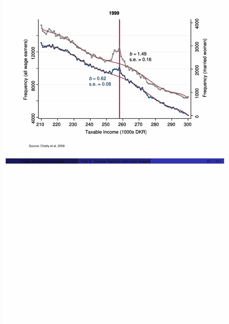
8/8/2019 Chetty - Public Economics Lectures
http://slidepdf.com/reader/full/chetty-public-economics-lectures 457/949
1 0 0 0
2 0 0 0
3 0 0 0
4 0
0 6 0 0 0
1 0 0 0 0
1 4 0 0 0
220 230 240 250 260 270 280 290 300210
Taxable Income (1000s DKR)
F r e q u e n c
y ( a l l w a g e e a r n e r
s )
F r e q u e n c y ( m a r r i e d w o m e
n )
b = 1.50s.e. = 0.21
b = 0.72s.e. = 0.09
1 0 0 0
2 0 0 0
3 0 0 0
4 0
0 6 0 0 0
1 0 0 0 0
1 4 0 0 0
220 230 240 250 260 270 280 290 300210
Taxable Income (1000s DKR)
F r e q u e n c
y ( a l l w a g e e a r n e r
s )
F r e q u e n c y ( m a r r i e d w o m e
n )
b = 1.50s.e. = 0.21
b = 0.72s.e. = 0.09
Source: Chetty et al. 2009
Public Economics Lectures ()Part 5: Income Taxation and Labor Supply 63 / 211
20012001

8/8/2019 Chetty - Public Economics Lectures
http://slidepdf.com/reader/full/chetty-public-economics-lectures 458/949
1 0 0 0
2 0 0 0
3 0 0 0
4 0 0 0
6
0 0 0
1
0 0 0 0
1 4 0 0 0
210 220 230 240 250 260 270 280 290 300
Taxable Income (1000s DKR)
F r e q u e n c y ( a l l w a g e e a r n e r
s )
F r e q u e n c y ( m a r r i e d w o m e
n )
b = 1.44s.e. = 0.20
b = 0.55s.e. = 0.10
1 0 0 0
2 0 0 0
3 0 0 0
4 0 0 0
6
0 0 0
1
0 0 0 0
1 4 0 0 0
210 220 230 240 250 260 270 280 290 300
Taxable Income (1000s DKR)
F r e q u e n c y ( a l l w a g e e a r n e r
s )
F r e q u e n c y ( m a r r i e d w o m e
n )
b = 1.44s.e. = 0.20
b = 0.55s.e. = 0.10
Source: Chetty et al. 2009
Public Economics Lectures ()Part 5: Income Taxation and Labor Supply 64 / 211
0 0
Married Women: Taxable Income Distribution at Middle Tax Cutoff
0 0
Married Women: Taxable Income Distribution at Middle Tax Cutoff

8/8/2019 Chetty - Public Economics Lectures
http://slidepdf.com/reader/full/chetty-public-economics-lectures 459/949
1 0 0
0 0
2 0 0 0 0
3 0 0 0 0
4 0 0 0
-50 -40 -30 -20 -10 0 10 20 30 40 50
Taxable Income Relative to Middle Bracket Cutoff
F r e q u e n c y
Excess mass (b ) = 0.06Standard error = 0.03
Predicted excess mass = 0.35Standard error = 0.02
1 0 0
0 0
2 0 0 0 0
3 0 0 0 0
4 0 0 0
-50 -40 -30 -20 -10 0 10 20 30 40 50
Taxable Income Relative to Middle Bracket Cutoff
F r e q u e n c y
Excess mass (b ) = 0.06Standard error = 0.03
Predicted excess mass = 0.35Standard error = 0.02
Source: Chetty et al. 2009
Public Economics Lectures ()Part 5: Income Taxation and Labor Supply 65 / 211
Observed Elasticity vs. Size of Tax ChangeAll Wage Earners
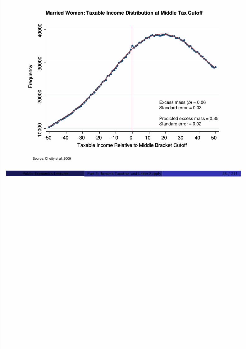
8/8/2019 Chetty - Public Economics Lectures
http://slidepdf.com/reader/full/chetty-public-economics-lectures 460/949
Log Change in Net-of-Tax Rate
O b s e r v e d
E l a s t i c i t i e s
0 10% 20% 30%5% 15% 25%
0
0.005
0.01
-0.005
Source: Chetty et al. 2009
Public Economics Lectures ()Part 5: Income Taxation and Labor Supply 66 / 211
Distribution of Net DeductionsDistribution of Net Deductions
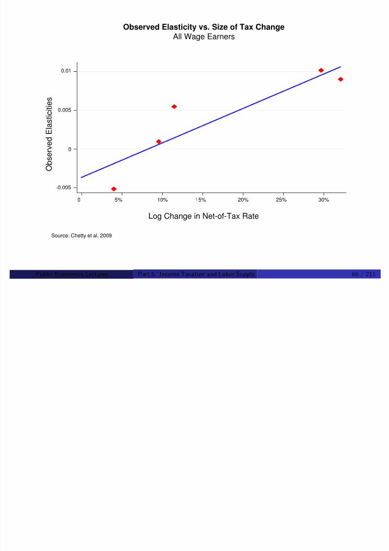
8/8/2019 Chetty - Public Economics Lectures
http://slidepdf.com/reader/full/chetty-public-economics-lectures 461/949
0
1 0
2 0
3 0
4 0
-50000 0 50000
Net Deduction (DKr)
F r
e q u e n c y
0
1 0
2 0
3 0
4 0
-50000 0 50000
Net Deduction (DKr)
F r
e q u e n c y
Source: Chetty et al. 2009
Indivs with non-wage income Indivs making pension contribs.
Public Economics Lectures ()Part 5: Income Taxation and Labor Supply 67 / 211
0 0
All Teachers
0 0
All Teachers

8/8/2019 Chetty - Public Economics Lectures
http://slidepdf.com/reader/full/chetty-public-economics-lectures 462/949
0
5 0 0
1 0 0 0
1 5
-50 -40 -30 -20 -10 0 10 20 30 40 50
Wage Earnings Relative to Statutory Kink (1000s DKR)
F
r e q u e n c y
0
5 0 0
1 0 0 0
1 5
-50 -40 -30 -20 -10 0 10 20 30 40 50
Wage Earnings Relative to Statutory Kink (1000s DKR)
F
r e q u e n c y
Source: Chetty et al. 2009
Public Economics Lectures ()Part 5: Income Taxation and Labor Supply 68 / 211
0 0 0
Teachers with Deductions > DKr 20,000
0 0 0
Teachers with Deductions > DKr 20,000

8/8/2019 Chetty - Public Economics Lectures
http://slidepdf.com/reader/full/chetty-public-economics-lectures 463/949
0
2 0 0 0
4 0
0 0
6 0 0 0
8 0 0
0
1 0 0
-50 -40 -30 -20 -10 0 10 20 30 40 50
Wage Earnings Relative to Statutory Kink (1000s DKR)
F
r e q u e n c y
0
2 0 0 0
4 0
0 0
6 0 0 0
8 0 0
0
1 0 0
-50 -40 -30 -20 -10 0 10 20 30 40 50
Wage Earnings Relative to Statutory Kink (1000s DKR)
F
r e q u e n c y
Source: Chetty et al. 2009
Public Economics Lectures ()Part 5: Income Taxation and Labor Supply 69 / 211
Electricians (3114), 2000
6 0
8 0
6 0
8 0
3 0 0
3 0 0
(b) Salesmen, 1996
(a) Electricians, 2000
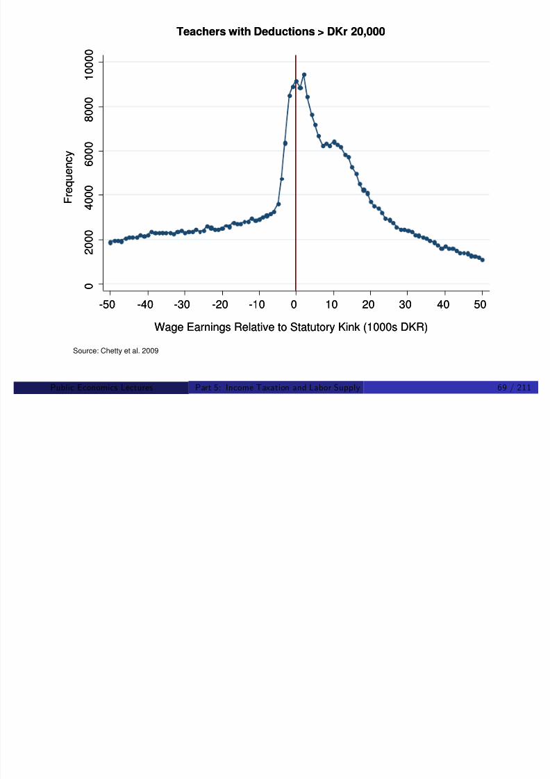
8/8/2019 Chetty - Public Economics Lectures
http://slidepdf.com/reader/full/chetty-public-economics-lectures 464/949
F
r e q u e n c y
Wage Earnings Relative to Top Bracket Cutoff
2 0
4 0
0
-100 -50 0 50 100
F
r e q u e n c y
Wage Earnings Relative to Top Bracket Cutoff (1000s DKr)
2 0
4 0
0
-100 -50 0 50 100
F
r e q u e n c y
1 0 0
2 0 0
Wage Earnings Relative to Top Bracket Cutoff
0
-100 -50 0 50 100
F
r e q u e n c y
1 0 0
2 0 0
Wage Earnings Relative to Top Bracket Cutoff (1000s DKr)
0
-100 -50 0 50 100
F r e q u e n c y
Wage Earnings Relative to Top Bracket Cutoff
0
5 0
1 0 0
1 5
0
-100 -50 0 50 100
(c) Nurses and Midwifes, 2001
F r e q u e n c y
Wage Earnings Relative to Top Bracket Cutoff (1000s DKr)
0
5 0
1 0 0
1 5
0
-100 -50 0 50 100
(d) Tellers and Clerks, 1998
F r e q u e n c y
Wage Earnings Relative to Top Bracket Cutoff (1000s DKr)
1 0 0
2 0 0
3 0 0
4 0 0
0
-100 -50 0 50 100
Source: Chetty et al. 2009
Public Economics Lectures ()Part 5: Income Taxation and Labor Supply 70 / 211
3 0
Modes of Occupation-Level Wage Earnings Distributions

8/8/2019 Chetty - Public Economics Lectures
http://slidepdf.com/reader/full/chetty-public-economics-lectures 465/949
0
1 0
2 0
-100 -50 0 50 100
F
r e q u e n c y
Modes of Wage Earnings Distributions Relative to Top Bracket Cutoff (1000s DKr)
Source: Chetty et al. 2009
Public Economics Lectures ()Part 5: Income Taxation and Labor Supply 71 / 211
0 0 0
Self-Employed: Taxable Income Distribution around Top Tax Cutoff
0 0 0
Self-Employed: Taxable Income Distribution around Top Tax Cutoff

8/8/2019 Chetty - Public Economics Lectures
http://slidepdf.com/reader/full/chetty-public-economics-lectures 466/949
0
2 0 0 0 0
4 0 0 0 0
6 0
-50 -40 -30 -20 -10 0 10 20 30 40 50
Excess mass (b ) = 18.42Standard error = 0.42
F
r e q u e n c y
Taxable Income Relative to Top Bracket Cutoff (1000s DKr)
0
2 0 0 0 0
4 0 0 0 0
6 0
-50 -40 -30 -20 -10 0 10 20 30 40 50
Excess mass (b ) = 18.42Standard error = 0.42
F
r e q u e n c y
Taxable Income Relative to Top Bracket Cutoff (1000s DKr)
Source: Chetty et al. 2009
Public Economics Lectures ()Part 5: Income Taxation and Labor Supply 72 / 211
2 0 0 0
Self-Employed: Taxable Income Distribution around Middle Tax Cutoff
2 0 0 0
Self-Employed: Taxable Income Distribution around Middle Tax Cutoff
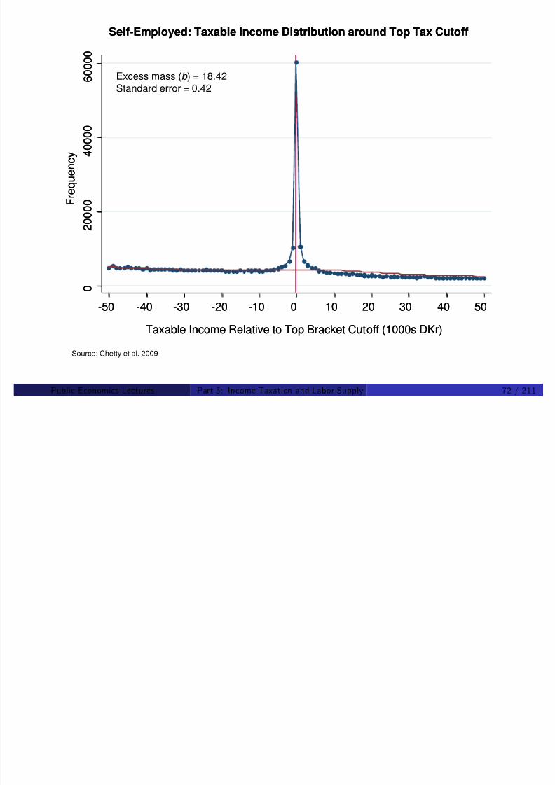
8/8/2019 Chetty - Public Economics Lectures
http://slidepdf.com/reader/full/chetty-public-economics-lectures 467/949
4 0 0 0
6 0 0 0
8 0 0 0
1 0 0 0
0
1 2
-50 -40 -30 -20 -10 0 10 20 30 40 50
Excess mass (b )= 1.44Standard error = 0.10
F
r e q u e n c y
Taxable Income Relative to Top Bracket Cutoff (1000s DKr)
4 0 0 0
6 0 0 0
8 0 0 0
1 0 0 0
0
1 2
-50 -40 -30 -20 -10 0 10 20 30 40 50
Excess mass (b )= 1.44Standard error = 0.10
F
r e q u e n c y
Taxable Income Relative to Top Bracket Cutoff (1000s DKr)
Source: Chetty et al. 2009
Public Economics Lectures ()Part 5: Income Taxation and Labor Supply 73 / 211
Chetty et al. 2009: Results
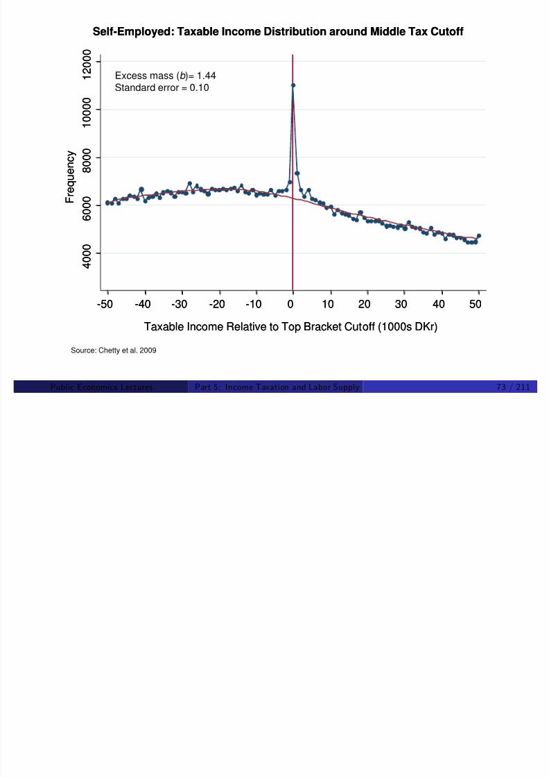
8/8/2019 Chetty - Public Economics Lectures
http://slidepdf.com/reader/full/chetty-public-economics-lectures 468/949
Search costs attenuate observed behavioral responses substantially
Firm responses and coordination critical for understanding behavior:individual and group elasticities may di¤er signi…cantly
NLBS models may …t data better if these factors are incorporated
Standard method of estimating elasticities using small tax reforms onsame data yields close-to-zero elasticity estimate
Public Economics Lectures ()Part 5: Income Taxation and Labor Supply 74 / 211
Estimates of Hours and Participation Elasticities

8/8/2019 Chetty - Public Economics Lectures
http://slidepdf.com/reader/full/chetty-public-economics-lectures 469/949
Return to simple model where we ignore non-linear budget set issues
Large literature in labor economics estimates e¤ects of taxes and
wages on hours worked and participation
Now discuss some estimates from this older literature
Public Economics Lectures ()Part 5: Income Taxation and Labor Supply 75 / 211
Negative Income Tax
Best way to resolve identi…cation problems: exogenously increase the

8/8/2019 Chetty - Public Economics Lectures
http://slidepdf.com/reader/full/chetty-public-economics-lectures 470/949
Best way to resolve identi…cation problems: exogenously increase themarginal tax rate
NIT experiment conducted in 1960s/70s in Denver, Seattle, and othercities
First major social experiment in U.S.
Provided lump-sum welfare grants G combined with a steep phaseoutrate τ (50%-70%)
Analysis by Rees (1974), Ashenfelter and Plant (1990), and others
Several groups, with randomization within each; approx. N = 75households in each group
Public Economics Lectures ()Part 5: Income Taxation and Labor Supply 76 / 211

8/8/2019 Chetty - Public Economics Lectures
http://slidepdf.com/reader/full/chetty-public-economics-lectures 471/949
Public Economics Lectures ()Part 5: Income Taxation and Labor Supply 77 / 211
NIT Experiments: Ashenfelter and Plant 1990
Present non-parametric evidence of labor supply e¤ects
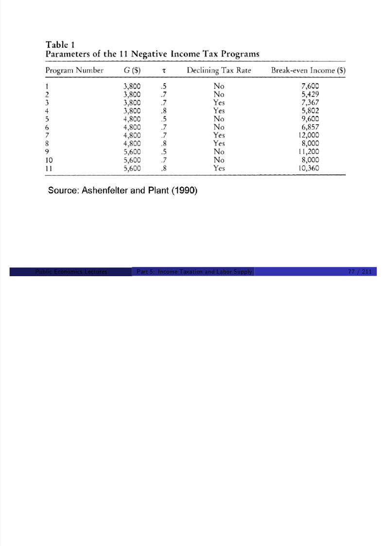
8/8/2019 Chetty - Public Economics Lectures
http://slidepdf.com/reader/full/chetty-public-economics-lectures 472/949
Present non parametric evidence of labor supply e¤ects
Compare implied bene…t payments to treated vs control households
Di¤erence in bene…t payments aggregates hours and participationresponses
This is the relevant parameter for expenditure calculations andpotentially for welfare analysis (revenue method of calculating DWL)
Shortcoming: approach does not decompose estimates into income
and substitution e¤ects
Hard to identify the key elasticity relevant for policy purposes andpredict labor supply e¤ect of other programs
Public Economics Lectures ()Part 5: Income Taxation and Labor Supply 78 / 211

8/8/2019 Chetty - Public Economics Lectures
http://slidepdf.com/reader/full/chetty-public-economics-lectures 473/949
Public Economics Lectures ()Part 5: Income Taxation and Labor Supply 79 / 211
NIT Experiments: Findings
Signi…cant labor supply response but small overall

8/8/2019 Chetty - Public Economics Lectures
http://slidepdf.com/reader/full/chetty-public-economics-lectures 474/949
Signi…cant labor supply response but small overall
Implied earnings elasticity for males around 0.1
Implied earnings elasticity for women around 0.5
Academic literature not careful to decompose response alongintensive and extensive margin
Response of women is concentrated along the extensive margin (canonly be seen in o¢cial govt. report)
Earnings of treated women who were working before the experimentdid not change much
Public Economics Lectures ()Part 5: Income Taxation and Labor Supply 80 / 211
Problems with Experimental Design
Estimates from NIT not considered credible due to several shortcomings:
S lf d i

8/8/2019 Chetty - Public Economics Lectures
http://slidepdf.com/reader/full/chetty-public-economics-lectures 475/949
1 Self reported earnings
Treatments had …nancial incentives to under-report earnings.Reported earnings not well correlated with actual payments!Lesson: need to match with administrative records
2 Selective attrition
After initial year, data was collected based on voluntary income reportsby families to qualify for the grant
Those in less generous groups/far above breakeven point had much lessincentive to report
Consequently attrition rates were much higher in these groups
!No longer a random sample of treatment + controls
3 Response might be smaller than real reform b/c of GE e¤ects
Public Economics Lectures ()Part 5: Income Taxation and Labor Supply 81 / 211
Social Experiments: Costs/Bene…ts

8/8/2019 Chetty - Public Economics Lectures
http://slidepdf.com/reader/full/chetty-public-economics-lectures 476/949
Cost of NIT experiments: around $1 billion (in today’s dollars)
Huge cost for a social experiment but trivial relative to budget of theUS federal government ($2 trillion)
Should the government do more experimentation? Potential bene…ts:
Narrow the standard error around estimates
Allow implementation of better tax and redistribution policy
Public Economics Lectures ()Part 5: Income Taxation and Labor Supply 82 / 211
Instrumental Variable Methods
8/8/2019 Chetty - Public Economics Lectures
http://slidepdf.com/reader/full/chetty-public-economics-lectures 477/949
Another strategy to overcome endogeneity is instrumenting for wagerate
Mroz (1987): often-cited survey/meta-analysis of earlier studies
Uses PSID to test widely-used IV’s for married women’s wage
l i = α + βw + γX + ε
w = θZ + µ
Uses Hausman speci…cation/overidenti…cation test to show that manyinstruments violate EZ ε = 0
Public Economics Lectures ()Part 5: Income Taxation and Labor Supply 83 / 211
Hausman Test

8/8/2019 Chetty - Public Economics Lectures
http://slidepdf.com/reader/full/chetty-public-economics-lectures 478/949
Suppose you can divide instrument set into those that are credibly
exogenous (Z ) and those that are questionable (Z )
Null hypothesis: both are exogenous
Alternative hypothesis: Z
is endogenous
Compute IV estimate of β with small and large instrument set andtest for equality of the coe¢cients
Note that is often a very lower power test (accept validity if instruments are weak)
Public Economics Lectures ()Part 5: Income Taxation and Labor Supply 84 / 211
Mroz 1987: Setup and Results
U b k d i bl “ dibl ”i t t

8/8/2019 Chetty - Public Economics Lectures
http://slidepdf.com/reader/full/chetty-public-economics-lectures 479/949
Uses background variables as credibly exogenous instruments
Parents’ education, wife’ age, education polynomials
Tests validity of labor market experience, average hourly earnings, andprevious reported wages
Rejects validity of all three
Shows that earlier estimates are highly fragile and unreliable
Contributed to emerging view that policy variation (e.g., taxes) wasnecessary to really identify these elasticities properly
Public Economics Lectures ()Part 5: Income Taxation and Labor Supply 85 / 211
Tax Reform Variation (Eissa 1995)
Modern studies use tax changes as “natural experiments”

8/8/2019 Chetty - Public Economics Lectures
http://slidepdf.com/reader/full/chetty-public-economics-lectures 480/949
Representative example: Eissa (1995)
Uses the Tax Reform Act of 1986 to identify the e¤ect of MTRs onlabor force participation and hours of married women
TRA 1986 cut top income MTR from 50% to 28% from 1986 to 1988
But did not signi…cantly change tax rates for the middle class
Substantially increased incentives to work of wives of high incomehusbands relative wives of middle income husbands
DD strategy: compare women in top 1% households (treatment) withwomen in 90th percentile and 75th percentile (controls)
Data: CPS, 1983-85 and 1989-91
Public Economics Lectures ()Part 5: Income Taxation and Labor Supply 86 / 211
8/8/2019 Chetty - Public Economics Lectures
http://slidepdf.com/reader/full/chetty-public-economics-lectures 481/949

8/8/2019 Chetty - Public Economics Lectures
http://slidepdf.com/reader/full/chetty-public-economics-lectures 482/949
Public Economics Lectures ()Part 5: Income Taxation and Labor Supply 88 / 211

8/8/2019 Chetty - Public Economics Lectures
http://slidepdf.com/reader/full/chetty-public-economics-lectures 483/949
Public Economics Lectures ()Part 5: Income Taxation and Labor Supply 89 / 211
Eissa 1995: Results

8/8/2019 Chetty - Public Economics Lectures
http://slidepdf.com/reader/full/chetty-public-economics-lectures 484/949
Participation elasticity around 0.4 but large standard errors
Hours elasticity of 0.6
Total elasticity (unconditional hours) is 0.4 + 0.6 = 1
Public Economics Lectures ()Part 5: Income Taxation and Labor Supply 90 / 211
Eissa 1995: Caveats

8/8/2019 Chetty - Public Economics Lectures
http://slidepdf.com/reader/full/chetty-public-economics-lectures 485/949
Does the common trends assumption hold?
Potential story biasing the result:
Trend toward “power couples” and thus DD might not be due to taxesIn the 1980s, professionals had non-working spousesIn the 1990s, professionals married to professionalsWhile for middle class, always married to working middle class wives
Problem: starting from very di¤erent levels for T and C groups
Liebman and Saez (2006) show that Eissa’s results are not robustusing admin data (SSA matched to SIPP)
Public Economics Lectures ()Part 5: Income Taxation and Labor Supply 91 / 211

8/8/2019 Chetty - Public Economics Lectures
http://slidepdf.com/reader/full/chetty-public-economics-lectures 486/949
Public Economics Lectures ()Part 5: Income Taxation and Labor Supply 92 / 211
Bianchi, Gudmundsson, and Zoega 2001
U “ ” I l d l
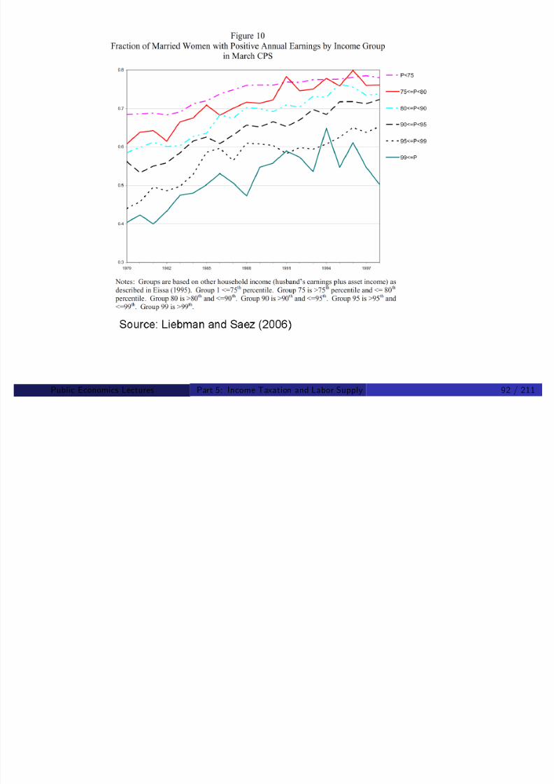
8/8/2019 Chetty - Public Economics Lectures
http://slidepdf.com/reader/full/chetty-public-economics-lectures 487/949
Use 1987 “no tax year” in Iceland as a natural experiment
In 1987-88, Iceland switched to a withholding-based tax system
Workers paid taxes on 1986 income in 1987; paid taxes on 1988
income in 1988; 1987 earnings never taxed
Data: individual tax returns matched with data on weeks worked frominsurance database
Random sample of 9,274 individuals who …led income tax-returns in1986-88
Public Economics Lectures ()Part 5: Income Taxation and Labor Supply 93 / 211

8/8/2019 Chetty - Public Economics Lectures
http://slidepdf.com/reader/full/chetty-public-economics-lectures 488/949
Public Economics Lectures ()Part 5: Income Taxation and Labor Supply 94 / 211

8/8/2019 Chetty - Public Economics Lectures
http://slidepdf.com/reader/full/chetty-public-economics-lectures 489/949
Public Economics Lectures ()Part 5: Income Taxation and Labor Supply 95 / 211

8/8/2019 Chetty - Public Economics Lectures
http://slidepdf.com/reader/full/chetty-public-economics-lectures 490/949
Public Economics Lectures ()Part 5: Income Taxation and Labor Supply 96 / 211
Bianchi, Gudmundsson, and Zoega 2001
Large, salient change: ∆ log(1 MTR ) 43%, much bigger than

8/8/2019 Chetty - Public Economics Lectures
http://slidepdf.com/reader/full/chetty-public-economics-lectures 491/949
most studies
Note that elasticities reported in paper are w.r.t. average tax rates:
εL,T /E =∑ (L87 LA)/LA
∑ T 86/
E 86
εE ,T /E =∑ (E 87 E A)/E A
∑ T 86/E 86
Estimates imply hours elasticity w.r.t. marginal tax rate of roughly
0.29
Is this a Frisch or Hicksian elasticity?
Public Economics Lectures ()Part 5: Income Taxation and Labor Supply 97 / 211
Responses to Low-Income Transfer Programs

8/8/2019 Chetty - Public Economics Lectures
http://slidepdf.com/reader/full/chetty-public-economics-lectures 492/949
Particular interest in treatment of low incomes in a progressive taxsystem: are they responsive to incentives?
Complicated set of transfer programs in US
In-kind: food stamps, Medicaid, public housing, job training, educationsubsidiesCash: TANF, EITC, SSI
P blic Economics Lect res ()Part 5 Income Ta ation and Labor S ppl 98 / 211
Overall Costs of Anti Poverty Programs
8/8/2019 Chetty - Public Economics Lectures
http://slidepdf.com/reader/full/chetty-public-economics-lectures 493/949
US government (fed+state and local) spent $520bn in 2002 onincome-tested programs
About 5% of GDP but 15% of $3.5 Trillion govt budget
(fed+state+local).
About 50% is health care (Medicaid)
Only $100 billion in cash (1% of GDP, or 20% of transfer spending)
P bli E i L t ()P t 5 I T ti d L b S l 99 / 211
1996 Welfare Reform
Largest change in welfare policy

8/8/2019 Chetty - Public Economics Lectures
http://slidepdf.com/reader/full/chetty-public-economics-lectures 494/949
Reform modi…ed AFDC cash welfare program to provide moreincentives to work by
1 Requiring recipients to go to job trainings
2 Limiting the duration for which families able to receive welfare
3 Reducing phase out to 66 cents of bene…ts per $1 earnings instead of 100% cli¤
Variation across states because Fed govt. gave block grants with
guidelines
EITC also expanded during this period: general shift from welfare to“workfare”
P bli E i L t ()P t 5 I T ti d L b S l 100 / 211
Monthly Welfare Case Loads: 1963-2000

8/8/2019 Chetty - Public Economics Lectures
http://slidepdf.com/reader/full/chetty-public-economics-lectures 495/949
P bli E i L t ()P t 5 I T ti d L b S l 101 / 211
Welfare Reform: Two Empirical Questions
I i did lf f ll i l b l

8/8/2019 Chetty - Public Economics Lectures
http://slidepdf.com/reader/full/chetty-public-economics-lectures 496/949
1 Incentives: did welfare reform actually increase labor supply
Test whether EITC expansions a¤ect labor supply
2 Bene…ts: did removing many people from transfer system reduce their
welfare?
How did consumption change?
Focus on single mothers, who were most impacted by reform
P bli E i L t ()P t 5 I T ti d L b S l 102 / 211
Behavioral Responses to the EITC
1 Phase in:

8/8/2019 Chetty - Public Economics Lectures
http://slidepdf.com/reader/full/chetty-public-economics-lectures 497/949
Substitution e¤ect: work more due to 40% inc. in net wageIncome e¤ect: work less!Net e¤ect: ambiguous; probably work more
2 Plateau:
Pure income e¤ect (no change in net wage)!Net e¤ect: work less
3 Phase out:
Substitution e¤ect: work less because reduces net wage to $0.80/hrIncome e¤ect: also make you work less!Net e¤ect: work less
Public Economics Lectures ()Part 5: Income Taxation and Labor Supply 103 / 211

8/8/2019 Chetty - Public Economics Lectures
http://slidepdf.com/reader/full/chetty-public-economics-lectures 498/949
Public Economics Lectures ()Part 5: Income Taxation and Labor Supply 104 / 211
Eissa and Liebman 1996
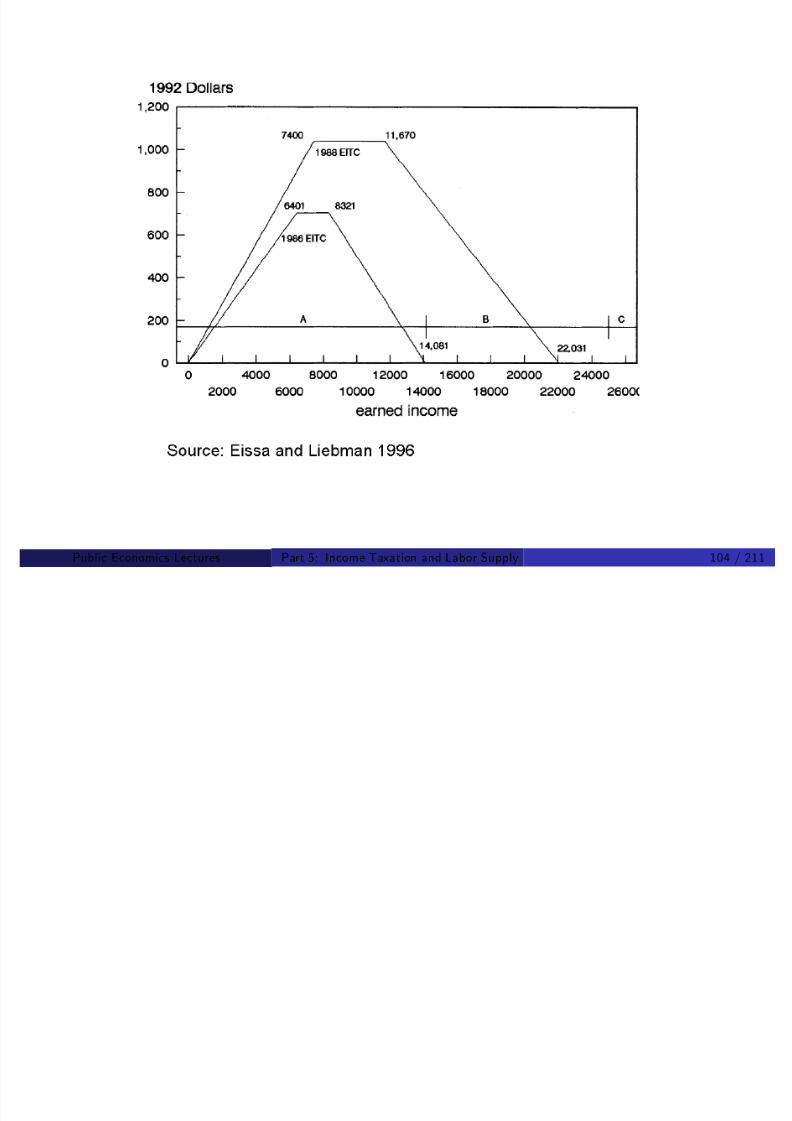
8/8/2019 Chetty - Public Economics Lectures
http://slidepdf.com/reader/full/chetty-public-economics-lectures 499/949
Study labor force participation of single mothers before/after 1986-7EITC expansion
Limitation: this expansion was relatively small
Di¤-in-Di¤ strategy:
Treatment group: women with kids
Control group: women without kids
Public Economics Lectures ()Part 5: Income Taxation and Labor Supply 105 / 211

8/8/2019 Chetty - Public Economics Lectures
http://slidepdf.com/reader/full/chetty-public-economics-lectures 500/949
Public Economics Lectures ()Part 5: Income Taxation and Labor Supply 106 / 211
Eissa and Liebman: Results

8/8/2019 Chetty - Public Economics Lectures
http://slidepdf.com/reader/full/chetty-public-economics-lectures 501/949
Find a small but signi…cant DD e¤ect: 2.4%
Note: the labor force participation for women with/without childrenare not great comparison groups (70% LFP vs. +90%)
Subsequent studies have used much bigger EITC expansions of themid 1990s
Also …nd positive e¤ects on labor force participation of singlewomen/single mothers
Public Economics Lectures ()Part 5: Income Taxation and Labor Supply 107 / 211
Meyer and Rosenbaum 2001
Exploit the much bigger 1990s expansion in EITC
Document dramatic (6 pp 10%) increase in LFP for single women

8/8/2019 Chetty - Public Economics Lectures
http://slidepdf.com/reader/full/chetty-public-economics-lectures 502/949
Document dramatic (6 pp, 10%) increase in LFP for single womenwith children around EITC expansion
No change for women without children
Problem: expansion took place at same time as welfare reform
Try to disentangle e¤ects of welfare waivers, changes in AFDC andstate taxes, etc. using state-level variation
Bottom line: elasticity of participation w.r.t. tax/transfer incentives issigni…cant
But no clear elasticity estimate to use as an input for optimal policy
Public Economics Lectures ()Part 5: Income Taxation and Labor Supply 108 / 211

8/8/2019 Chetty - Public Economics Lectures
http://slidepdf.com/reader/full/chetty-public-economics-lectures 503/949
Public Economics Lectures ()Part 5: Income Taxation and Labor Supply 109 / 211
1
Employment Rates for Single Women with and without Children
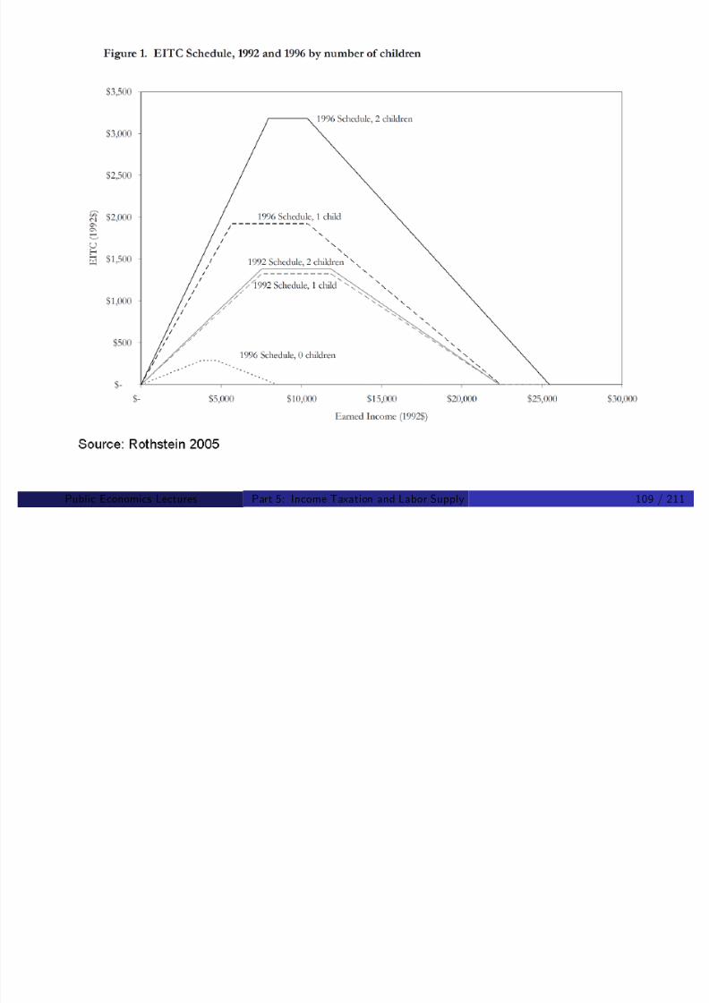
8/8/2019 Chetty - Public Economics Lectures
http://slidepdf.com/reader/full/chetty-public-economics-lectures 504/949
. 7
. 8
. 9
E m p l o y m e n t R a t e
1984 1986 1988 1990 1992 1994 1996
Year
Children No Children
Source: Meyer and Rosenbaum 2001
Public Economics Lectures ()Part 5: Income Taxation and Labor Supply 110 / 211
Meyer and Rosenbaum 2001
Analyze the introduction of EITC and Welfare waivers for the period1984-1996 using CPS data
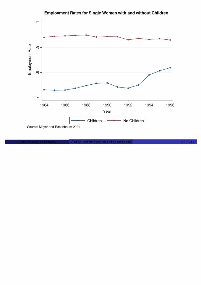
8/8/2019 Chetty - Public Economics Lectures
http://slidepdf.com/reader/full/chetty-public-economics-lectures 505/949
Identi…cation strategy: compare single mothers to single womenwithout kids
Key covariates in regression model:
EITC
AFDC bene…ts
Medicaid
Waivers
Training
Child Care
Public Economics Lectures ()Part 5: Income Taxation and Labor Supply 111 / 211
Meyer and Rosenbaum 2001
From 1984-1996, the extra increase in single mom’s relative to single

8/8/2019 Chetty - Public Economics Lectures
http://slidepdf.com/reader/full/chetty-public-economics-lectures 506/949
From 1984 1996, the extra increase in single mom s relative to single
women without kids is explained by:
1 EITC expansion (60%)
2 Welfare max bene…t reduction (AFDC and food stamps) (25%)
3 Medicaid if work (-10%) (insigni…cant and wrong sign)
4 Welfare waivers (time limits) 15%
5 Child care and training: 15%
Public Economics Lectures ()Part 5: Income Taxation and Labor Supply 112 / 211
Eissa and Hoynes 2004
EITC based on family rather than individual income

8/8/2019 Chetty - Public Economics Lectures
http://slidepdf.com/reader/full/chetty-public-economics-lectures 507/949
Study married couples with low earnings, recognizing that EITCreduces their incentive to work
Married women with husband earning $10-15K are in the phase-outrange and face high MTR’s
Payroll tax 15%
EITC phase-out 20%
State and federal income tax 0-20%
Similar identi…cation strategy: compare those with and without kids
Public Economics Lectures ()Part 5: Income Taxation and Labor Supply 113 / 211
Eissa and Hoynes: Results
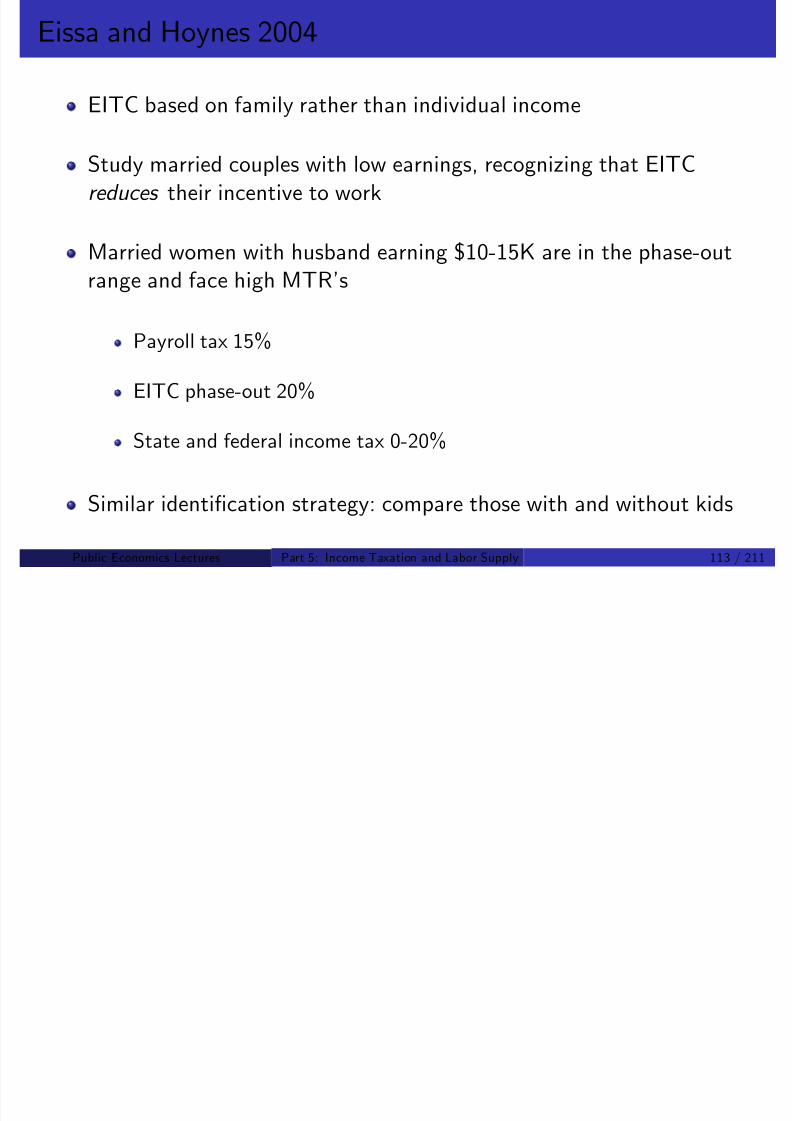
8/8/2019 Chetty - Public Economics Lectures
http://slidepdf.com/reader/full/chetty-public-economics-lectures 508/949
Conclude that EITC expansions between 1984 and 1996:
Increased married men’s labor force participation by 0.2%
Reduced married women’s labor force participation by>
1%
Implies that the EITC is e¤ectively subsidizing married mothers tostay at home and reducing total labor supply for married households
Public Economics Lectures ()Part 5: Income Taxation and Labor Supply 114 / 211
Meyer and Sullivan 2004

8/8/2019 Chetty - Public Economics Lectures
http://slidepdf.com/reader/full/chetty-public-economics-lectures 509/949
Examine the consumption patterns of single mothers and theirfamilies from 1984–2000 using CEX data
Question: did single mothers’ consumption fall because they lostwelfare bene…ts and were forced to work?
Public Economics Lectures ()Part 5: Income Taxation and Labor Supply 115 / 211
Total Consumption: Single Mothers 1984-2000

8/8/2019 Chetty - Public Economics Lectures
http://slidepdf.com/reader/full/chetty-public-economics-lectures 510/949
Public Economics Lectures ()Part 5: Income Taxation and Labor Supply 116 / 211
Relative Consumption: single women with/without children

8/8/2019 Chetty - Public Economics Lectures
http://slidepdf.com/reader/full/chetty-public-economics-lectures 511/949
Public Economics Lectures ()Part 5: Income Taxation and Labor Supply 117 / 211
Relative Consumption: married vs. single mothers

8/8/2019 Chetty - Public Economics Lectures
http://slidepdf.com/reader/full/chetty-public-economics-lectures 512/949
Public Economics Lectures ()Part 5: Income Taxation and Labor Supply 118 / 211

8/8/2019 Chetty - Public Economics Lectures
http://slidepdf.com/reader/full/chetty-public-economics-lectures 513/949
Other Behavioral Responses to Transfer Programs

8/8/2019 Chetty - Public Economics Lectures
http://slidepdf.com/reader/full/chetty-public-economics-lectures 514/949
Bitler, Gelbach, and Hoynes (2005): distributional e¤ects are veryimportant in understanding welfare programs because of nonlinearitiesin bc ! cannot just look at means
Other studies have examined e¤ects of low-income assistance
programs on other margins such as family structure (divorce rate,number of kids) and …nd limited e¤ects
Empirical work on tagging and in-kind programs is more limited and isan important area for further research
Public Economics Lectures ()Part 5: Income Taxation and Labor Supply 120 / 211
Changing Elasticities: Blau and Kahn 2007
Identify elasticities from 1980-2000 using grouping instrument

8/8/2019 Chetty - Public Economics Lectures
http://slidepdf.com/reader/full/chetty-public-economics-lectures 515/949
1 De…ne cells (year/age/gender/education) and compute mean wages2 Instrument for actual wage with mean wage
Identify purely from group-level variation, which is less contaminated
by individual endogenous choice
Result: total hours elasticity (including int + ext margin) shrank from0.4 in 1980 to 0.2 today
Interpretation: elasticities shrink as women become more attached tothe labor force
Public Economics Lectures ()Part 5: Income Taxation and Labor Supply 121 / 211
Summary of Static Labor Supply Literature
1 Small elasticities for prime-age males
Probably institutional restrictions, need for one income, etc. prevent a

8/8/2019 Chetty - Public Economics Lectures
http://slidepdf.com/reader/full/chetty-public-economics-lectures 516/949
short-run response
2 Larger responses for workers who are less attached to labor force
Married women, low incomes, retirees
3 Responses driven by extensive margin
Ext margin (participation) elasticity around 0.2
Int margin (hours) elasticity close 0
Public Economics Lectures ()Part 5: Income Taxation and Labor Supply 122 / 211
Intertemporal Models and the MaCurdy Critique
What parameter do reduced-form regressions of labor supply onwages or taxes identify?

8/8/2019 Chetty - Public Economics Lectures
http://slidepdf.com/reader/full/chetty-public-economics-lectures 517/949
MaCurdy critique: reduced-form studies did not identify anyparameter of interest in a dynamic model
Instead, estimate a mix of income e¤ects, intertemporal substitutione¤ects, and compensated wage elasticities
MaCurdy (1981) develops a structural estimation method (two stagebudgeting) to identify preference parameters in a life-cycle model of
labor supply
Chetty (2006) presents a simple exposition of two-stage budgeting
Public Economics Lectures ()Part 5: Income Taxation and Labor Supply 123 / 211
Life Cycle Model of Labor Supply
General model is of the form:

8/8/2019 Chetty - Public Economics Lectures
http://slidepdf.com/reader/full/chetty-public-economics-lectures 518/949
U (c 0, .., c T , l 0, .., l T )
s.t. A0 +∑ w t l t /(1 + r )t ∑ c t /(1 + r )t (λ)
First order conditions:
U l t (c 0, .., c T , l 0, .., l T ) + λw t /(1 + r )t = 0
U c t (c 0, .., c T , l 0, .., l T ) + λ/(1 + r )t = 0
In the general case, l t (A0, w 0, .., w T ) same as the multi-good choice –
no generic results
Public Economics Lectures ()Part 5: Income Taxation and Labor Supply 124 / 211
Life Cycle Model: Time Separability
By assuming time separability can rewrite the problem as:
U
T
∑ β ( l )

8/8/2019 Chetty - Public Economics Lectures
http://slidepdf.com/reader/full/chetty-public-economics-lectures 519/949
U = ∑ t =0 βt u (c t , l t )
Leads to simpler …rst order conditions
l t
: βt u l t
+ λw t /(1 + r )t = 0
c t : βt u c t + λ/(1 + r )t = 0
Combining yields: u l (l t ) = w t u c
Intratemporal f.o.c. same as in static model
Intertemporal f.o.c.: u c t /u c t +1 = β(1 + r )
Public Economics Lectures ()Part 5: Income Taxation and Labor Supply 125 / 211
Dynamic Life Cycle Model: Policy Rulesλ = u c 0 is the marginal utility of initial consumption
The two …rst order conditions imply that
l l ( λ/(β(1 ))t )
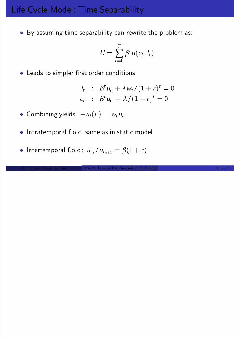
8/8/2019 Chetty - Public Economics Lectures
http://slidepdf.com/reader/full/chetty-public-economics-lectures 520/949
l t = l (w t ,λ/( β(1 + r ))t )c t = c (w t , λ/( β(1 + r ))t )
Current labor and consumption choice depends on current w t
All other wage rates and initial wealth enter only through the budgetconstraint multiplier λ (MaCurdy 1981)
Easy to see for separable utility:
u (c , l ) = u (c ) v (l )
) v 0(l t ) = λw t /[ β(1 + r )]t
) l t = v 01(λw t /[ β(1 + r )]t )
Su¢ciency of λ greatly simpli…es solution to ITLS model
Public Economics Lectures ()Part 5: Income Taxation and Labor Supply 126 / 211
Dynamic Life Cycle Model: Frisch Elasticity
Frisch intertemporal labor supply elasticity de…ned as:
δ = (w t
lt
)∂l
∂ t
jλ
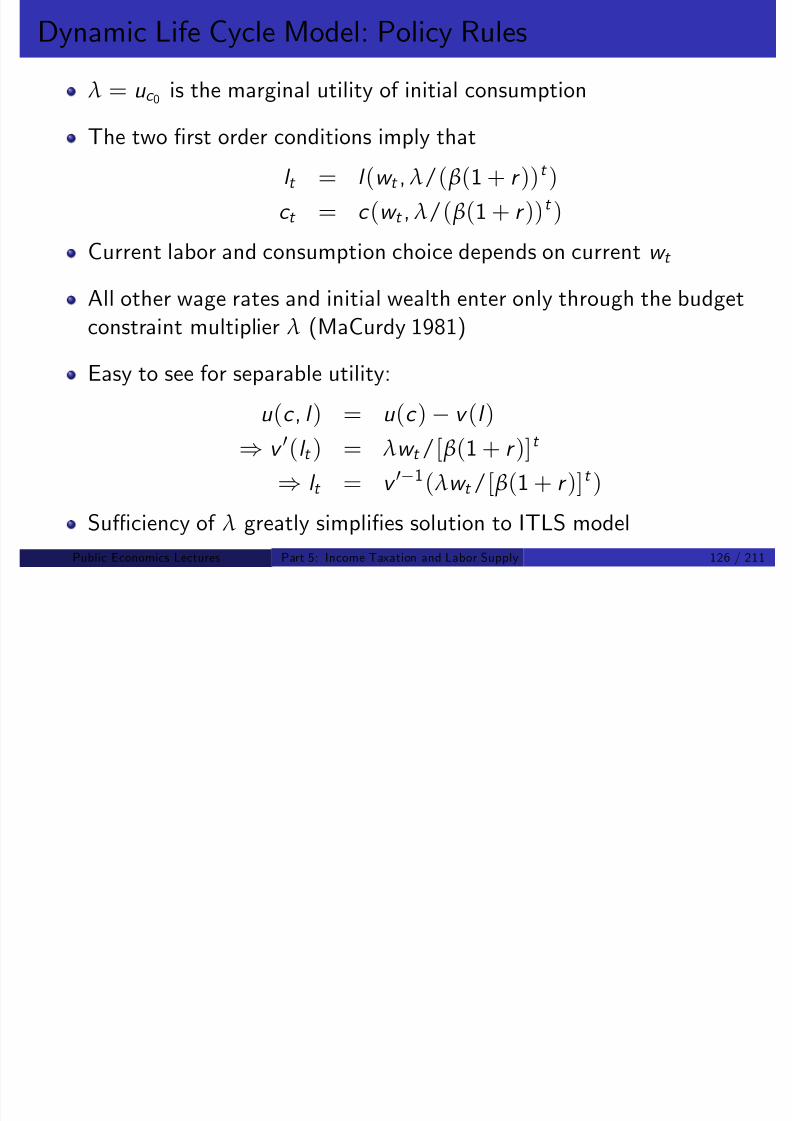
8/8/2019 Chetty - Public Economics Lectures
http://slidepdf.com/reader/full/chetty-public-economics-lectures 521/949
l t ∂w t
Experiment: change wage rate in one period only, holding all otherwages, and consumption pro…le constant
Can show that δ > 0: work more today to take advantage of temporarily higher wage
In separable case:
l t = v 01(λw t /[ β(1 + r )]t )
)∂l
∂w t jλ =
λ
β(1 + r )t v 00(l t )> 0
Public Economics Lectures ()Part 5: Income Taxation and Labor Supply 127 / 211

8/8/2019 Chetty - Public Economics Lectures
http://slidepdf.com/reader/full/chetty-public-economics-lectures 522/949

8/8/2019 Chetty - Public Economics Lectures
http://slidepdf.com/reader/full/chetty-public-economics-lectures 523/949
Public Economics Lectures ()Part 5: Income Taxation and Labor Supply 129 / 211
Frisch vs. Compensated vs. Uncompensated Elasticities
Frisch elasticity Compensated static elasticity
Compensated static elasticity Uncompensated static elasticity
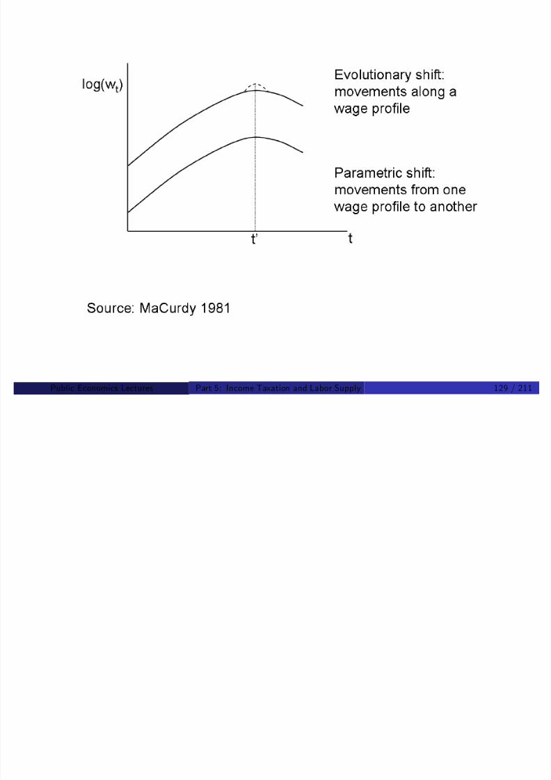
8/8/2019 Chetty - Public Economics Lectures
http://slidepdf.com/reader/full/chetty-public-economics-lectures 524/949
Compensated static elasticity: changing wages in all periods butkeeping utility constant
Uncompensated static elasticity: changing wages in each period with
no compensation
First inequality is due to inter-temporal substitution:
When wage increases only in 1 period, substitute labor from otherperiods toward this period
When it increases in all periods, do not have this motive
Second inequality is due to income e¤ects (as in static model)
Public Economics Lectures ()Part 5: Income Taxation and Labor Supply 130 / 211
Frisch vs. Compensated vs. Uncompensated Elasticities
Frisch elasticity Compensated static elasticity
Compensated static elasticity Uncompensated static elasticity

8/8/2019 Chetty - Public Economics Lectures
http://slidepdf.com/reader/full/chetty-public-economics-lectures 525/949
Compensated static elasticity Uncompensated static elasticity
Without income e¤ects, all three elasticities are equal
Otherwise inequalities are strict
Di¤erence in elasticities related to anticipated vs. unanticipatedchanges
Looney and Singhal (2007) exploit this logic to identify Frisch elasticity
Frisch elasticity is of central interest for calibration of macro businesscycle models
Public Economics Lectures ()Part 5: Income Taxation and Labor Supply 131 / 211
Structural Estimates: MaCurdy 1983 and Pencavel 2002
MaCurdy (1983)

8/8/2019 Chetty - Public Economics Lectures
http://slidepdf.com/reader/full/chetty-public-economics-lectures 526/949
Structural estimate using panel data for men and within-person wagevariationFind both Frisch and compensated wage elasticity of around 0.15But wage variation is not exogenous
Pencavel (2002)
Instruments with trade balance interacted with schooling and ageFrisch elasticity: 0.2Uncompensated wage elasticity: 0-0.2
Public Economics Lectures ()Part 5: Income Taxation and Labor Supply 132 / 211
Card Critique of ITLS models
Critiques value of ITLS model
F il t l i t i ti i h lif l

8/8/2019 Chetty - Public Economics Lectures
http://slidepdf.com/reader/full/chetty-public-economics-lectures 527/949
Fails to explain most variation in hours over lifecycle
Sheds little light on pro…le-shift elasticities that we care about
Di¢cult to identify key parameters
Exempli…es structural vs. reduced-form divide in appliedmicroeconomics
Tradeo¤ between credible identi…cation and identi…cation of structural
parameters
Public Economics Lectures ()Part 5: Income Taxation and Labor Supply 133 / 211
Blundell, Duncan, and Meghir 1998
Good combination of structural and reduced form methods on labor
supply

8/8/2019 Chetty - Public Economics Lectures
http://slidepdf.com/reader/full/chetty-public-economics-lectures 528/949
supply
Argue against standard DD approach, where treatment/controlgroups are endogenously de…ned based on income
E.g., reduced tax rate may pull households into that tax group
Need group de…nitions that are stable over time
Use birth cohort (decade) interacted with education (e.g. high schoolor more)
Public Economics Lectures ()Part 5: Income Taxation and Labor Supply 134 / 211
Blundell, Duncan, and Meghir 1998
Construct group-level labor supply measures for women

8/8/2019 Chetty - Public Economics Lectures
http://slidepdf.com/reader/full/chetty-public-economics-lectures 529/949
Measure how labor supply co-varies with wages rates net of taxes inthe UK in 1980s
Importantly, tax reforms during this period a¤ected groups verydi¤erently
Use consumption data as a control for permanent income
Can therefore obtain a structurally interpretable (λ constant) estimate
Public Economics Lectures ()Part 5: Income Taxation and Labor Supply 135 / 211

8/8/2019 Chetty - Public Economics Lectures
http://slidepdf.com/reader/full/chetty-public-economics-lectures 530/949
Public Economics Lectures ()Part 5: Income Taxation and Labor Supply 136 / 211
Blundell, Duncan, and Meghir: Results
Compensated wage elasticities: 0.15-0.3, depending on number of kids
Vi ll i ¤

8/8/2019 Chetty - Public Economics Lectures
http://slidepdf.com/reader/full/chetty-public-economics-lectures 531/949
Virtually no income e¤ects
Identi…cation assumption is common trends across cohort/ed groups
However, reforms in 80s went in opposite directions at di¤erent times
!Secular trends cannot explain everything
See Pencavel (1986) and Blundell and MaCurdy (1999) for additionalITLS estimates
Public Economics Lectures ()Part 5: Income Taxation and Labor Supply 137 / 211
Intertemporal Substitution: High Frequency Studies
Recent literature focuses on groups such as cab drivers with highly‡exible and well measured labor supply
8/8/2019 Chetty - Public Economics Lectures
http://slidepdf.com/reader/full/chetty-public-economics-lectures 532/949
Camerer et al. 1997: examine how variation across days in wage ratefor cab drivers (arising from variation in waiting times) correlates withhours worked
Striking …nding: strong negative e¤ect
Interpret this as “target earning” – strongly contradicts standardintertemporal labor supply model
Would imply counterintuitive e¤ects for temporary tax changes
Public Economics Lectures ()Part 5: Income Taxation and Labor Supply 138 / 211
8/8/2019 Chetty - Public Economics Lectures
http://slidepdf.com/reader/full/chetty-public-economics-lectures 533/949
Public Economics Lectures ()Part 5: Income Taxation and Labor Supply 139 / 211
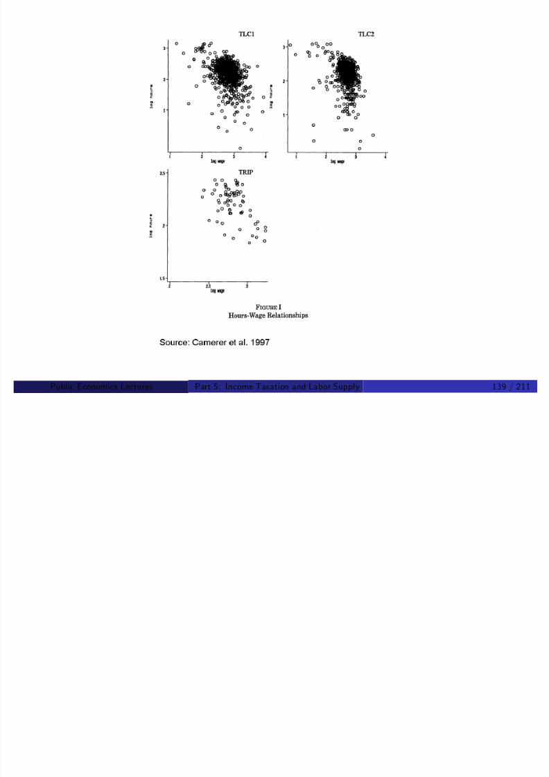
8/8/2019 Chetty - Public Economics Lectures
http://slidepdf.com/reader/full/chetty-public-economics-lectures 534/949
Public Economics Lectures ()Part 5: Income Taxation and Labor Supply 140 / 211
Farber 2005: Division Bias
Argues that Camerer et al. evidence of target earning behavior isdriven by econometric problems
Camerer et al regression speci…cation:
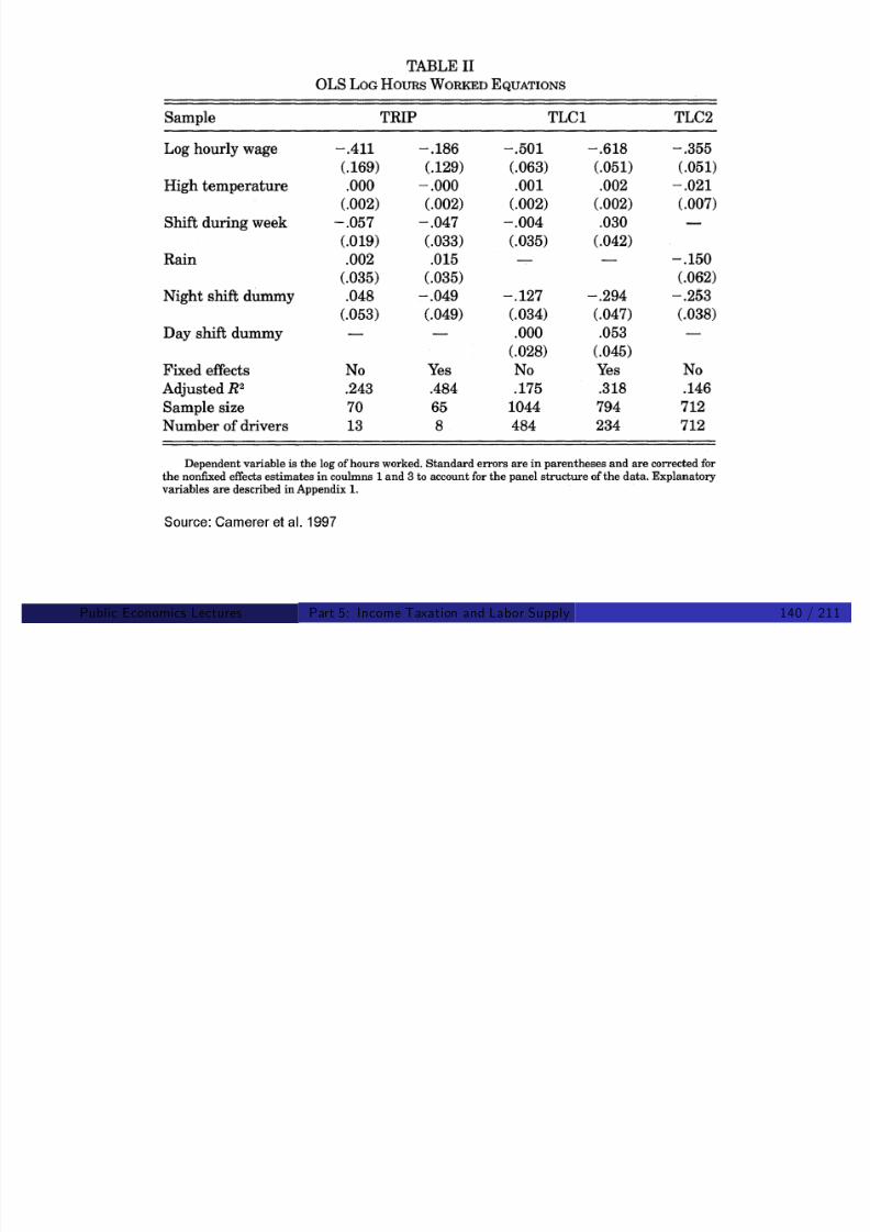
8/8/2019 Chetty - Public Economics Lectures
http://slidepdf.com/reader/full/chetty-public-economics-lectures 535/949
Camerer et al. regression speci…cation:
hit = α + βe it /hit + εit
Camerer et al. recognize this and try to instrument with average dailywage for each individual’s wage
But there may be a random component to hours at the group level(e.g., some days people just randomly report many hours on the job)
! Spuriously …nd a negative association between average daily wageand average hours
Public Economics Lectures ()Part 5: Income Taxation and Labor Supply 141 / 211
Farber: Alternative TestFarber’s alternative test for target earnings: hazard model
Quit = f (cum_hours , cum_inc )
Result: main determinant of quitting is hours worked, NOT
8/8/2019 Chetty - Public Economics Lectures
http://slidepdf.com/reader/full/chetty-public-economics-lectures 536/949
q gcumulative income
Rejects target earning, but does not yield ITLS estimate
Other studies …nd positive ITLS
Bicycle messengers (Fehr and Goette 2007 randomized experiment)Stadium vendors (Oettinger 1999: vendors show up more to highattendance games)
But structural parameters estimated in these studies are not of directinterest to macro models or public …nance because they are too highfrequency
Public Economics Lectures ()Part 5: Income Taxation and Labor Supply 142 / 211
Manoli and Weber 2009
Use variation in retirement bene…ts as a function of job tenure inAustria to estimate Frisch elasticity

8/8/2019 Chetty - Public Economics Lectures
http://slidepdf.com/reader/full/chetty-public-economics-lectures 537/949
jAustria to estimate Frisch elasticity
Question: how much do people delay retirement in order to get higher(anticipated) bene…ts?
Dataset: administrative panel for full population of Austria, 1980-2005
Rough estimate of Frisch elasticity: 0.2 at annual level
Public Economics Lectures ()Part 5: Income Taxation and Labor Supply 143 / 211
Lump-Sum Severance Payments at Retirement
. 7
5
1
a l a r y
. 7
5
1
a l a r y

8/8/2019 Chetty - Public Economics Lectures
http://slidepdf.com/reader/full/chetty-public-economics-lectures 538/949
0
. 3 3
3
. 5
F r a c t i o n
o f L a s t Y e a r ' s S
0 5 10 15 20 25 30Years of Tenure at Retirement
0
. 3 3
3
. 5
F r a c t i o n
o f L a s t Y e a r ' s S
0 5 10 15 20 25 30Years of Tenure at Retirement
Source: Manoli and Weber 2009
Public Economics Lectures ()Part 5: Income Taxation and Labor Supply 144 / 211
6 0 0 0
u a l s
Quarterly Frequency
Distribution of Tenure at Retirement
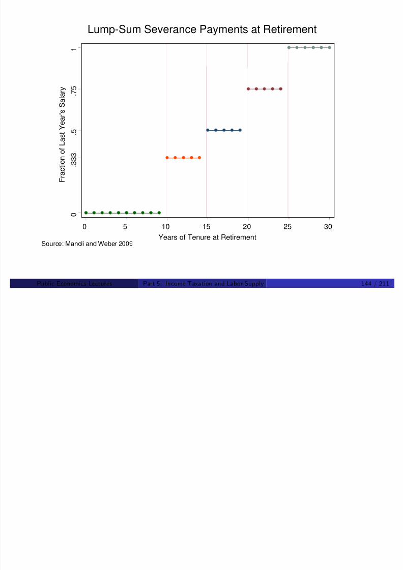
8/8/2019 Chetty - Public Economics Lectures
http://slidepdf.com/reader/full/chetty-public-economics-lectures 539/949
0
2 0 0 0
4 0 0 0
N u m b e r o f I n d i v i d
10 15 20 25
Years of Tenure at RetirementSource: Manoli and Weber 2009
Public Economics Lectures ()Part 5: Income Taxation and Labor Supply 145 / 211
Taxable Income Elasticities
Modern public …nance literature focuses on taxable income elasticities
instead of hours/participation elasticities

8/8/2019 Chetty - Public Economics Lectures
http://slidepdf.com/reader/full/chetty-public-economics-lectures 540/949
Two main reasons
1 Convenient su¢cient statistic for all distortions created by income tax
system (Feldstein 1999)
2 Data availability: taxable income is precisely measured in tax returndata
Good overview of this literature: Saez et al. 2009
Public Economics Lectures ()Part 5: Income Taxation and Labor Supply 146 / 211
US Income Taxation: Trends
The biggest changes in MTRs are at the top
1 [Kennedy tax cuts]: 91% to 70% in ’63-65

8/8/2019 Chetty - Public Economics Lectures
http://slidepdf.com/reader/full/chetty-public-economics-lectures 541/949
2 [Reagan I, ERTA 81]: 70% to 50% in ’81-82
3 [Reagan II, TRA 86]: 50% to 28% in ’86-88
4 [Bush I tax increase]: 28% to 31% in ’91
5 [Clinton tax increase]: 31% to 39.6% in ’93
6 [Bush Tax cuts]: 39.6% to 35% in ’01-03
Public Economics Lectures ()Part 5: Income Taxation and Labor Supply 147 / 211
Saez 2004: Long-Run Evidence
Compares top 1% relative to the bottom 99%
Bottom 99% real income increases up to early 1970s and stagnates
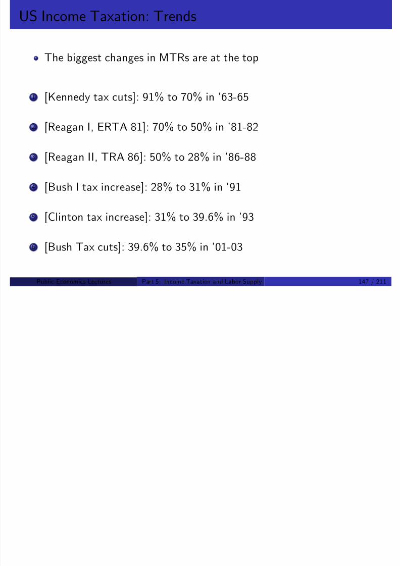
8/8/2019 Chetty - Public Economics Lectures
http://slidepdf.com/reader/full/chetty-public-economics-lectures 542/949
since then
Top 1% increases slowly up to the early 1980s and then increases
dramatically up to year 2000.
Corresponds to the decrease in MTRs
Pattern exempli…es general theme of this literature: large responsesfor top earners, no response for rest of the population
Public Economics Lectures ()Part 5: Income Taxation and Labor Supply 148 / 211
$25,000
$30,000
$35,000
$40,000
25%
30%
35%
40%
Bottom 99% Tax Units
x R a t
e

8/8/2019 Chetty - Public Economics Lectures
http://slidepdf.com/reader/full/chetty-public-economics-lectures 543/949
$0
$5,000
$10,000
$15,000
$20,000
5%Marginal Tax Rate Average Income5%Marginal Tax Rate Average Income5%Marginal Tax Rate Average Income
0%
10%
15%
20%
5%
Source: Saez 2004
M a r g i n a l T a x
1 9 6 0
1 9 6 2
1 9 6 4
1 9 6 6
1 9 6 8
1 9 7 0
1 9 7 2
1 9 7 4
1 9 7 6
1 9 7 8
1 9 8 0
1 9 8 2
1 9 8 4
1 9 8 6
1 9 8 8
1 9 9 0
1 9 9 2
1 9 9 4
1 9 9 6
1 9 9 8
2 0 0 0
Public Economics Lectures ()Part 5: Income Taxation and Labor Supply 149 / 211
Top 1% Tax Units
50%
60%
70%
80%
x R a t
e
$500,000
$600,000
$700,000
$800,000
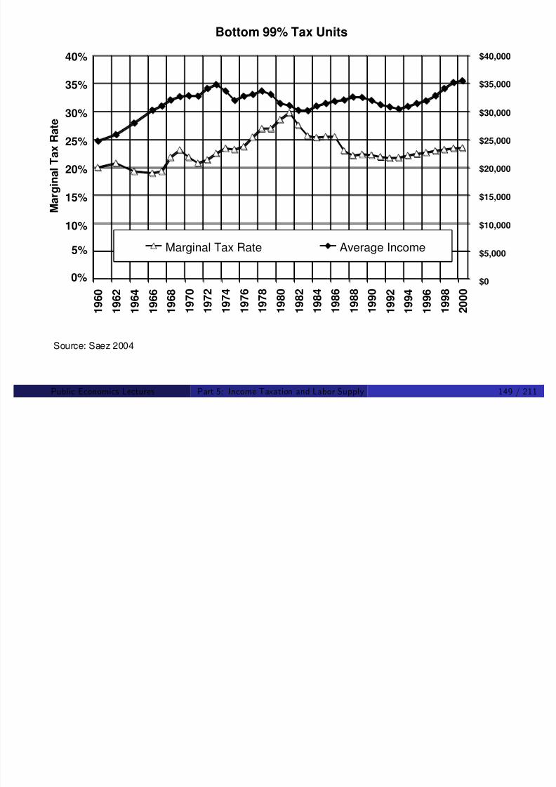
8/8/2019 Chetty - Public Economics Lectures
http://slidepdf.com/reader/full/chetty-public-economics-lectures 544/949
20%
30%
40%
1 9 6 0
1 9 6 2
1 9 6 4
1 9 6 6
1 9 6 8
1 9 7 0
1 9 7 2
1 9 7 4
1 9 7 6
1 9 7 8
1 9 8 0
1 9 8 2
1 9 8 4
1 9 8 6
1 9 8 8
1 9 9 0
1 9 9 2
1 9 9 4
1 9 9 6
1 9 9 8
2 0 0 0
M a r g i n a l T a x
$0
$100,000
$200,000
$300,000
$400,000
5%Marginal Tax Rate Average Income5%Marginal Tax Rate Average Income5%Marginal Tax Rate Average Income10%
Source: Saez 2004
0%
Public Economics Lectures ()Part 5: Income Taxation and Labor Supply 150 / 211
Feldstein 1995
First study of taxable income: Lindsey (1987) using cross-sectionsaround 1981 reform

8/8/2019 Chetty - Public Economics Lectures
http://slidepdf.com/reader/full/chetty-public-economics-lectures 545/949
Limited data and serious econometric problems
Feldstein (1995) estimates the e¤ect of TRA86 on taxable income for
top earners
Constructs three income groups based on income in 1985
Looks at how incomes and MTR evolve from 1985 to 1988 forindividuals in each group using panel
Public Economics Lectures ()Part 5: Income Taxation and Labor Supply 151 / 211

8/8/2019 Chetty - Public Economics Lectures
http://slidepdf.com/reader/full/chetty-public-economics-lectures 546/949
Feldstein: Results
Feldstein obtains very high elasticities (above 1) for top earners

8/8/2019 Chetty - Public Economics Lectures
http://slidepdf.com/reader/full/chetty-public-economics-lectures 547/949
Feldstein obtains very high elasticities (above 1) for top earners
Implication: we were on the wrong side of the La¤er curve for the rich
Cutting tax rates would raise revenue
Public Economics Lectures ()Part 5: Income Taxation and Labor Supply 153 / 211
Feldstein: Econometric Criticisms
DD can give very biased results when elasticity di¤er by groups
Suppose that the middle class has a zero elasticity so that
( M )

8/8/2019 Chetty - Public Economics Lectures
http://slidepdf.com/reader/full/chetty-public-economics-lectures 548/949
∆ log(z M ) = 0
Suppose high income individuals have an elasticity of e so that
∆ log(z H ) = e ∆ log(1 τ H )
Suppose tax change for high is twice as large:
∆ log(1 τ M ) = 10% and ∆ log(1 τ H ) = 20%
Estimated elasticity e = e 20%020%10% = 2e
Public Economics Lectures ()Part 5: Income Taxation and Labor Supply 154 / 211
Feldstein: Econometric Criticisms
Sample size: results driven by very few observations (Slemrod 1996)
A t C ll (1999) li t lt l T d t t

8/8/2019 Chetty - Public Economics Lectures
http://slidepdf.com/reader/full/chetty-public-economics-lectures 549/949
Auten-Carroll (1999) replicate results on larger Treasury dataset
Find a smaller elasticity: 0.65
Di¤erent trends across income groups (Goolsbee 1998)
Triple di¤erence that nets out di¤erential prior trends yields elasticity<0.4 for top earners
Public Economics Lectures ()Part 5: Income Taxation and Labor Supply 155 / 211
Slemrod: Shifting vs. “Real” Responses
Slemrod (1996) studies “anatomy” of the behavioral response
underlying change in taxable income

8/8/2019 Chetty - Public Economics Lectures
http://slidepdf.com/reader/full/chetty-public-economics-lectures 550/949
Shows that large part of increase is driven by shift between C corpincome to S corp income
Looks like a supply side story but government is actually losing revenueat the corporate tax level
Shifting across tax bases not taken into account in Feldstein e¢ciencycost calculations
Public Economics Lectures ()Part 5: Income Taxation and Labor Supply 156 / 211
10%
12%
14%
16%
18%
Wages S-Corp. Partner. Sole P. Dividends Interest Other
8/8/2019 Chetty - Public Economics Lectures
http://slidepdf.com/reader/full/chetty-public-economics-lectures 551/949
FIGURE 7
The Top 1% Income Share and Composition, 1960-2000
Source: Saez 2004
0%
2%
4%
6%
8%
1 9 6 0
1 9 6 2
1 9 6 4
1 9 6 6
1 9 6 8
1 9 7 0
1 9 7 2
1 9 7 4
1 9 7 6
1 9 7 8
1 9 8 0
1 9 8 2
1 9 8 4
1 9 8 6
1 9 8 8
1 9 9 0
1 9 9 2
1 9 9 4
1 9 9 6
1 9 9 8
2 0 0 0
Public Economics Lectures ()Part 5: Income Taxation and Labor Supply 157 / 211
Goolsbee: Intertemporal Shifting
Goolsbee (2000) hypothesizes that top earners’ ability to retimeincome drives much of observed responses
Analogous to identi…cation of Frisch elasticity instead of compensated

8/8/2019 Chetty - Public Economics Lectures
http://slidepdf.com/reader/full/chetty-public-economics-lectures 552/949
elasticitiy
Regression speci…cation:
TLI = α + β1 log(1 tax t ) + β2 log(1 tax t +1)
Long run e¤ect is β1 + β2
Uses ExecuComp data to study e¤ects of the 1993 Clinton taxincrease on executive pay
Public Economics Lectures ()Part 5: Income Taxation and Labor Supply 158 / 211

8/8/2019 Chetty - Public Economics Lectures
http://slidepdf.com/reader/full/chetty-public-economics-lectures 553/949
Public Economics Lectures ()Part 5: Income Taxation and Labor Supply 159 / 211
Goolsbee 2000
Most a¤ected groups (income>$250K) had a surge in income in 1992(when reform was announced) relative to 1991 followed by a sharp
drop in 1993
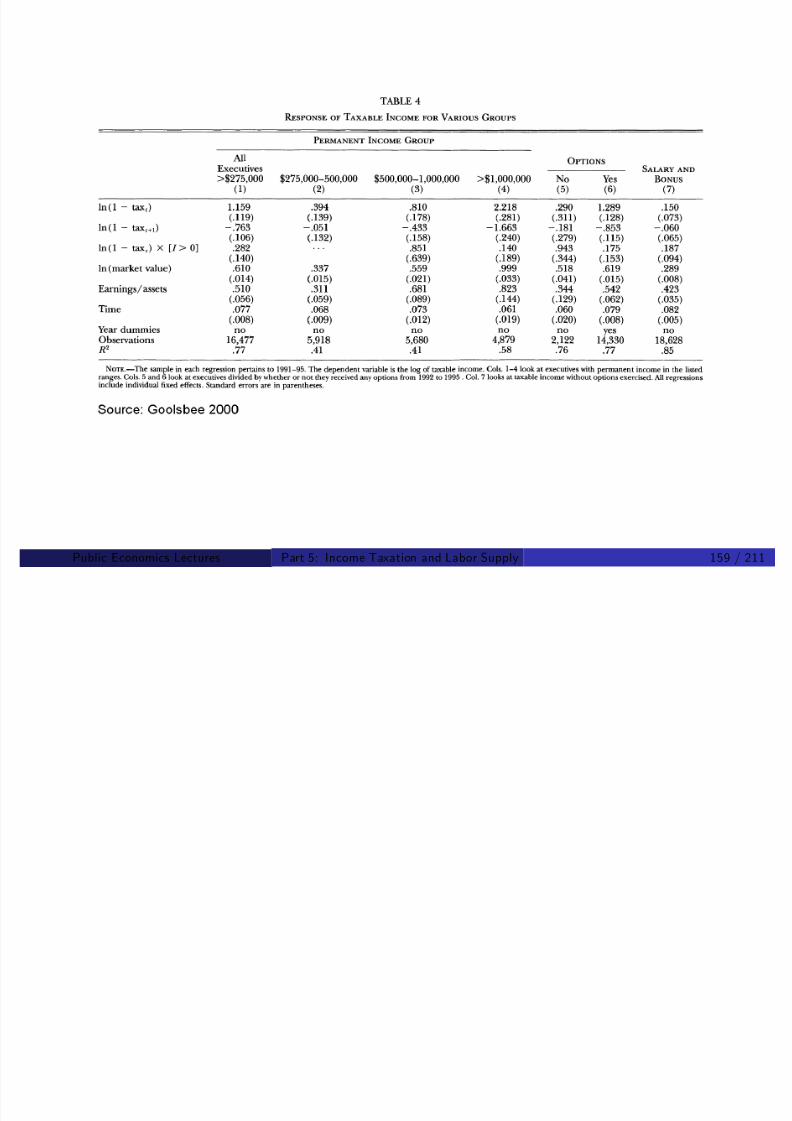
8/8/2019 Chetty - Public Economics Lectures
http://slidepdf.com/reader/full/chetty-public-economics-lectures 554/949
Simple DD estimate would …nd a large e¤ect here, but it would bepicking up pure re-timing
Concludes that long run e¤ect is 20x smaller than substitution e¤ect
E¤ects driven almost entirely by retiming exercise of options
Long run elasticity <0.4 and likely close to 0
Public Economics Lectures ()Part 5: Income Taxation and Labor Supply 160 / 211
Gruber and Saez 2002
First study to examine taxable income responses for generalpopulation, not just top earners
Use data from 1979-1991 on all tax changes available rather than a
single reform
S

8/8/2019 Chetty - Public Economics Lectures
http://slidepdf.com/reader/full/chetty-public-economics-lectures 555/949
Simulated instruments methodology
Step 1: Simulate tax rates based on period t income and characteristics
MTR P t +3 = f t +3(y t , X t )
MTR t +3 = f t +3(y t +3, X t +3)
Step 2 […rst stage]: Regress log(1 MTR t +3) log(1 MTR t ) onlog(1 MTR P
t +3) log(1 MTR t )
Step 3 [second stage]: Regress ∆ log TI on predicted value from …rststage
Isolates changes in laws (f t ) as the only source of variation in tax rates
Public Economics Lectures ()Part 5: Income Taxation and Labor Supply 161 / 211

8/8/2019 Chetty - Public Economics Lectures
http://slidepdf.com/reader/full/chetty-public-economics-lectures 556/949
Public Economics Lectures ()Part 5: Income Taxation and Labor Supply 162 / 211

8/8/2019 Chetty - Public Economics Lectures
http://slidepdf.com/reader/full/chetty-public-economics-lectures 557/949
Evidence from Danish Tax Reforms
e E a r n i n g s
Observed Earnings Responses to Small Tax Reforms
0 . 5
1

8/8/2019 Chetty - Public Economics Lectures
http://slidepdf.com/reader/full/chetty-public-economics-lectures 558/949
% R e s i d u a l C h a
n g e i n W a g e
% Residual Change in Net-of-Tax Wage Rate ∆log(1-t)
- 1
. 5
- 1
- 0 . 5
0
-4 -2 0 2 4 6
Source: Chetty et al. 2009
Public Economics Lectures ()Part 5: Income Taxation and Labor Supply 164 / 211
Imbens et al. 2001: Income E¤ects
Estimate income e¤ects using lottery winnings
Survey responses matched with administrative data on earnings from
Social Security Administration

8/8/2019 Chetty - Public Economics Lectures
http://slidepdf.com/reader/full/chetty-public-economics-lectures 559/949
Divide sample into three subgroups:
1
Losers [N = 259]: “season ticket holders” who won $100-$5K
2 Winners [N = 237]: anyone who won prizes of $22K to $9.7 mil
3 Big Winners [N = 43]: winners of prizes >$2 mil total ($100K/yr)
Estimate marginal propensity to earn out of unearned income of d [wl ]/dy = 0.1
Public Economics Lectures ()Part 5: Income Taxation and Labor Supply 165 / 211
8/8/2019 Chetty - Public Economics Lectures
http://slidepdf.com/reader/full/chetty-public-economics-lectures 560/949
Public Economics Lectures ()Part 5: Income Taxation and Labor Supply 166 / 211
Taxable Income Literature: Summary
Large responses for the rich, mostly intertemporal substitution andshifting
Responses among lower incomes small at least in short run

8/8/2019 Chetty - Public Economics Lectures
http://slidepdf.com/reader/full/chetty-public-economics-lectures 561/949
Perhaps not surprising if they have little ‡exibility to change earnings
Pattern con…rmed in many settings (e.g. Kopczuk 2009 - Polish ‡attax reform)
But many methdological problems remain to be resolved
Econometric issues: mean reversion, appropriate counterfactuals
Which elasticity is being identi…ed?
Public Economics Lectures ()Part 5: Income Taxation and Labor Supply 167 / 211
Macro Evidence
Macroeconomists estimate/calibrate elasticities by examininglong-term trends/cross-country comparisons
Identi…cation more questionable but estimates perhaps more relevantt l li ti f i t t
8/8/2019 Chetty - Public Economics Lectures
http://slidepdf.com/reader/full/chetty-public-economics-lectures 562/949
to long-run policy questions of interest
Use aggregate hours data and aggregate measures of taxes (average
tax rates)
But highly in‡uential in calibration of macroeconomic models
Macro models require high elasticities to …t both business cycle andcross-country data
Public Economics Lectures ()Part 5: Income Taxation and Labor Supply 168 / 211
Prescott 2004
Uses data on hours worked by country in 1970 and 1995 for 7 OECDcountries
Technique to identify elasticity: calibration of GE model
Rough intuition: posit a labor supply model, e.g.
8/8/2019 Chetty - Public Economics Lectures
http://slidepdf.com/reader/full/chetty-public-economics-lectures 563/949
u (c , l ) = c l 1+1/ε
1 + 1/ε
Finds that elasticity of ε = 1.2 best matches time series andcross-sectional patterns
Note that this is analogous to a regression without controls for other
variables
Results veri…ed in subsequent calibrations by Rogerson and othersusing more data
Public Economics Lectures ()Part 5: Income Taxation and Labor Supply 169 / 211
8/8/2019 Chetty - Public Economics Lectures
http://slidepdf.com/reader/full/chetty-public-economics-lectures 564/949
Public Economics Lectures ()Part 5: Income Taxation and Labor Supply 170 / 211
Davis and Henrekson 2005
Run regressions of hours worked on tax variables with various controls

8/8/2019 Chetty - Public Economics Lectures
http://slidepdf.com/reader/full/chetty-public-economics-lectures 565/949
Some panel evidence, but primarily cross-sectional
Separate intensive and extensive margin responses
Public Economics Lectures ()Part 5: Income Taxation and Labor Supply 171 / 211

8/8/2019 Chetty - Public Economics Lectures
http://slidepdf.com/reader/full/chetty-public-economics-lectures 566/949
Public Economics Lectures ()Part 5: Income Taxation and Labor Supply 172 / 211
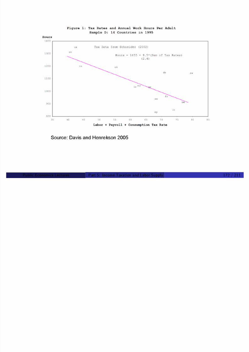
8/8/2019 Chetty - Public Economics Lectures
http://slidepdf.com/reader/full/chetty-public-economics-lectures 567/949
Public Economics Lectures ()Part 5: Income Taxation and Labor Supply 173 / 211
Reconciling Micro and Macro Estimates
Recent interest in reconciling micro and macro elasticity estimates
Three potential explanations
1 Statistical Bias: regulations culture di¤ers in countries with higher tax
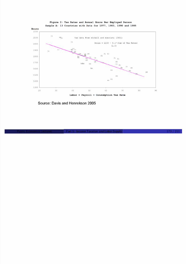
8/8/2019 Chetty - Public Economics Lectures
http://slidepdf.com/reader/full/chetty-public-economics-lectures 568/949
Statistical Bias: regulations, culture di¤ers in countries with higher taxrates [Alesina, Glaeser, Sacerdote 2005]
2
Extensive vs Intensive margin [Rogerson and Wallenius 2008]
L = Nhd log L
d (1 τ )=
d log N
d (1 τ )+
d log h
d (1 τ )>
d log h
d (1 τ )
3 Optimization frictions: short run vs. long run [Chetty 2009]
Public Economics Lectures ()Part 5: Income Taxation and Labor Supply 174 / 211
Optimization Frictions
Many frictions may cause agents to deviate from unconstrainedoptimum, e.g. adjustment costs or inattention
These frictions may attenuate short-run responses to tax reforms
Chetty (2009) asks two questions
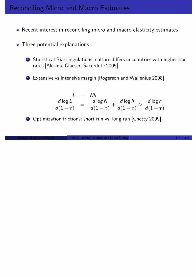
8/8/2019 Chetty - Public Economics Lectures
http://slidepdf.com/reader/full/chetty-public-economics-lectures 569/949
Chetty (2009) asks two questions
1 Can frictions quantitatively explain micro-macro puzzle and other
puzzles in labor supply literature?
2 Given frictions, what can we say about the “structural” elasticity?
Structural elasticity controls long run responses (e.g. Europe vs US)
Example: calculate utility loss from ignoring tax changes underneoclassical model with ε = 0.5
Public Economics Lectures ()Part 5: Income Taxation and Labor Supply 175 / 211

8/8/2019 Chetty - Public Economics Lectures
http://slidepdf.com/reader/full/chetty-public-economics-lectures 570/949
Public Economics Lectures ()Part 5: Income Taxation and Labor Supply 176 / 211
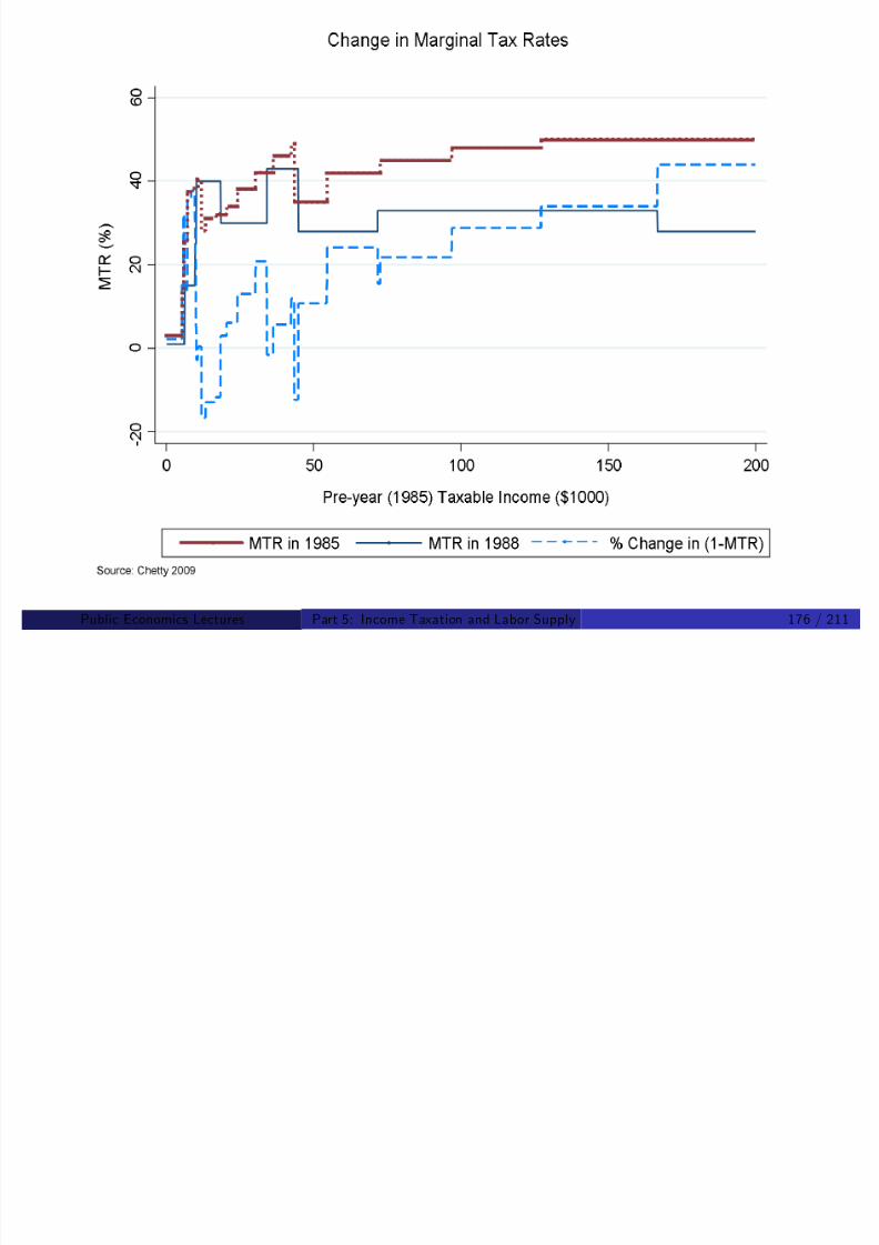
8/8/2019 Chetty - Public Economics Lectures
http://slidepdf.com/reader/full/chetty-public-economics-lectures 571/949
Public Economics Lectures ()Part 5: Income Taxation and Labor Supply 177 / 211

8/8/2019 Chetty - Public Economics Lectures
http://slidepdf.com/reader/full/chetty-public-economics-lectures 572/949
Public Economics Lectures ()Part 5: Income Taxation and Labor Supply 178 / 211
Setup
Consider a static demand model; results hold in dynamic model
N individuals with quasilinear utility over two goods:
u i (x , y ) = y + ai
x 11/ε
1 1/ε
Agent i ’s optimal demand for good x :

8/8/2019 Chetty - Public Economics Lectures
http://slidepdf.com/reader/full/chetty-public-economics-lectures 573/949
x i (p ) = (ai
p )ε
) log x i (p ) = α ε log p + v i
where v i = αi α denotes i ’s deviation from mean demand
Under orthogonality condition Ev i jp = 0,
ε = E log x 1 E log x 0log p 1 log p 0
!Observed response to price increase (p 0 to p 1) identi…es ε.
Public Economics Lectures ()Part 5: Income Taxation and Labor Supply 179 / 211
Optimization Frictions: Examples
Agent pays adjustment cost k i to change consumption
Demand set optimally at initial price p 0
Let x (p ) denote observed demand at price p
De…ne observed elasticity estimated from price increase as
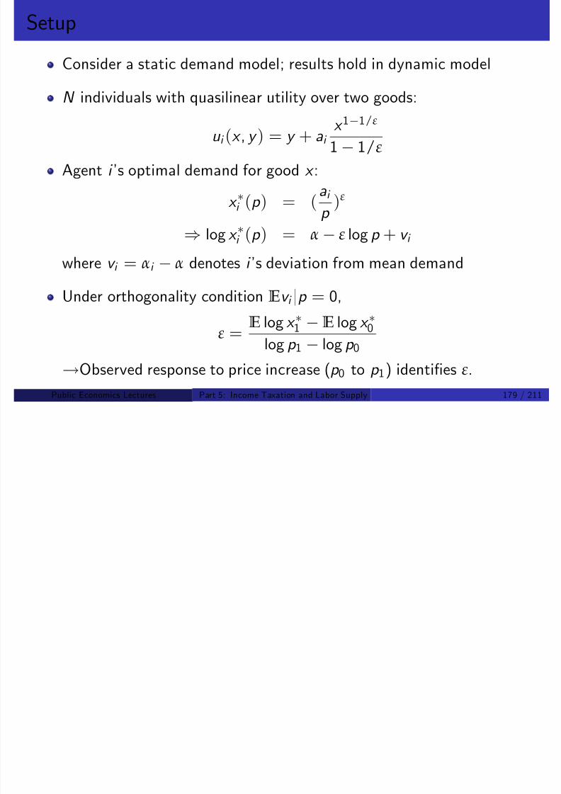
8/8/2019 Chetty - Public Economics Lectures
http://slidepdf.com/reader/full/chetty-public-economics-lectures 574/949
y p
b ε =E log x 1 E log x 0
log p 1
log p 0
Observed elasticity confounds structural elasticity ε with adjustmentcost distribution:
b ε = P (∆u i > k i )ε
Behavioral example: price misperception ep (p )
b ε = εE log ep (p 1) E log ep (p 0)
log p 1 log p 0
Public Economics Lectures ()Part 5: Income Taxation and Labor Supply 180 / 211
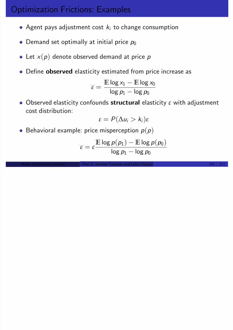
8/8/2019 Chetty - Public Economics Lectures
http://slidepdf.com/reader/full/chetty-public-economics-lectures 575/949
Optimization Frictions
Restriction on φ: Utility loss from deviations is less than exogenousthreshold δ:
U (x i ) U (x
i + φi ) < δpx
i
Frictions make agents deviate from optimal behavior as long as utilitycosts are not too large

8/8/2019 Chetty - Public Economics Lectures
http://slidepdf.com/reader/full/chetty-public-economics-lectures 576/949
costs are not too large
This restriction generates a class of models around nominal model
Includes adjustment cost models, inattention, etc.
A δ class of models maps price to a choice set X (p , δ) instead of a
single point x (p )
Public Economics Lectures ()Part 5: Income Taxation and Labor Supply 182 / 211
Construction of Choice Set
146
147
148
149
150
151
146
147
148
149
150
151
u ( x t
)
N pt xDÝ pt Þ

8/8/2019 Chetty - Public Economics Lectures
http://slidepdf.com/reader/full/chetty-public-economics-lectures 577/949
6 8 10 12 14 16 18 20 226 8 10 12 14 16 18 20 22
140
141
142
143
144
145
140
141
142
143
144
145
Demand (x t )
U t i l i t y
X Ý pt ,NÞ
Source: Chetty 2009
Public Economics Lectures ()Part 5: Income Taxation and Labor Supply 183 / 211
2 4
2.6
2.8
3.0ε = 1
n d ( l o g x t )
Identification with Optimization Frictions

8/8/2019 Chetty - Public Economics Lectures
http://slidepdf.com/reader/full/chetty-public-economics-lectures 578/949
0.4
1.8
2.0
2.2
2.4
0.6 0.8 1.4 1.6 1.81log(pA)
1.2log(pB)
l o g d e m a n
log price (log pt)Source: Chetty 2009
Public Economics Lectures ()Part 5: Income Taxation and Labor Supply 184 / 211

8/8/2019 Chetty - Public Economics Lectures
http://slidepdf.com/reader/full/chetty-public-economics-lectures 579/949
2.4
2.6
2.8
3.0ε = 1
n d ( l o g x t )
Identification with Optimization Frictions

8/8/2019 Chetty - Public Economics Lectures
http://slidepdf.com/reader/full/chetty-public-economics-lectures 580/949
0.4
1.8
2.0
2.2
2.4
0.6 0.8 1.4 1.6 1.81log(pA)
1.2log(pB)
l o g d e m a
log price (log pt)Source: Chetty 2009
Public Economics Lectures ()Part 5: Income Taxation and Labor Supply 186 / 211
2.4
2.6
2.8
3.0ε = 1
a n d ( l o g x t )
Identification with Optimization Frictions
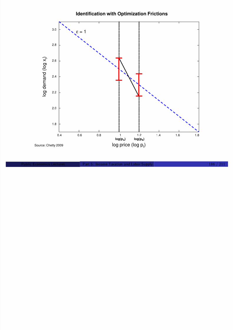
8/8/2019 Chetty - Public Economics Lectures
http://slidepdf.com/reader/full/chetty-public-economics-lectures 581/949
0.4
1.8
2.0
2.2
0.6 0.8 1.4 1.6 1.81log(pA)
1.2log(pB)
l o g d e m a
log price (log pt)Source: Chetty 2009
Public Economics Lectures ()Part 5: Income Taxation and Labor Supply 187 / 211
Bounds on Elasticities
Multiple observed elasticitiesb ε can be generated by a model with agiven structural elasticity when δ > 0
C l l i l l l i i i i i h b d

8/8/2019 Chetty - Public Economics Lectures
http://slidepdf.com/reader/full/chetty-public-economics-lectures 582/949
Conversely, multiple structural elasticities consistent with an observed b ε
Objective: derive bounds (εL, εU ) on smallest and largest structuralelasticities consistent with b ε
Public Economics Lectures ()Part 5: Income Taxation and Labor Supply 188 / 211
2 6
2.8
3
3.2
3.4
3.6
Calculation of Bounds on Structural Elasticity
a n d ( l o g x t )

8/8/2019 Chetty - Public Economics Lectures
http://slidepdf.com/reader/full/chetty-public-economics-lectures 583/949
1.8
2
2.2
2.4
2.6
0.2 0.4 0.6 0.8 1.2 1.6 1.8 2 2.21log(pA)
1.4log(pB)
l o g d e m a
log price (log pt)Source: Chetty 2009
Public Economics Lectures ()Part 5: Income Taxation and Labor Supply 189 / 211
2 6
2.8
3
3.2
3.4
3.6
a) Upper Bound on Structural Elasticity
a n d ( l o g x t )
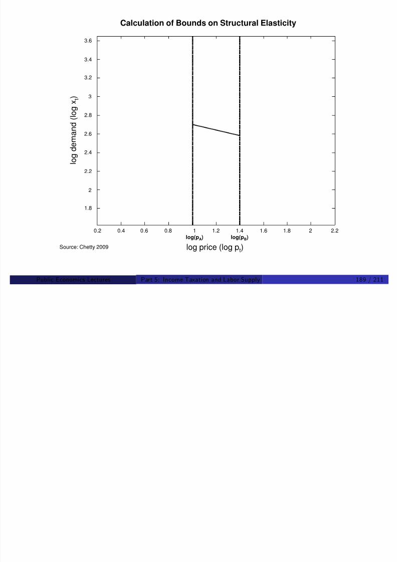
8/8/2019 Chetty - Public Economics Lectures
http://slidepdf.com/reader/full/chetty-public-economics-lectures 584/949
1.8
2
2.2
2.4
2.6
0.2 0.4 0.6 0.8 1.2 1.6 1.8 2 2.21log(pA)
1.4log(pB)
l o g d e m a
log price (log pt)Source: Chetty 2009
Public Economics Lectures ()Part 5: Income Taxation and Labor Supply 190 / 211
2.6
2.8
3
3.2
3.4
3.6
a n d ( l o g x t )
b) Lower Bound on Structural Elasticity

8/8/2019 Chetty - Public Economics Lectures
http://slidepdf.com/reader/full/chetty-public-economics-lectures 585/949
1.8
2
2.2
2.4
2.6
0.2 0.4 0.6 0.8 1.2 1.6 1.8 2 2.21log(pA)
1.4log(pB)
l o g d e m a
log price (log pt)Source: Chetty 2009
Public Economics Lectures ()Part 5: Income Taxation and Labor Supply 191 / 211
Bounds on Elasticity with Optimization Frictions
For small δ, the range of structural elasticities consistent with anobserved elasticity b ε in a δ class of models is approximately
[ b ε +4δ
(∆ log p )2(1 ρ), b ε +
4δ
(∆ log p )2(1 + ρ)]

8/8/2019 Chetty - Public Economics Lectures
http://slidepdf.com/reader/full/chetty-public-economics-lectures 586/949
where ρ = (1 +1
2
b ε
δ(∆ log p )2)1/2
Maps an observed elasticity ε, size of price change ∆ log p , and degreeof optimization frictions δ to bounds on ε.
Bounds shrink with (∆ log p )2
Public Economics Lectures ()Part 5: Income Taxation and Labor Supply 192 / 211
Application to Taxation and Labor Supply
Calculate bounds on taxable income elasticity using intensive-marginestimates from 20 recent studies
Assume δ = 1%

8/8/2019 Chetty - Public Economics Lectures
http://slidepdf.com/reader/full/chetty-public-economics-lectures 587/949
Assume δ = 1%
Ignore statistical imprecision for simplicity here
Text shows bounds for 95% con…dence interval
Public Economics Lectures ()Part 5: Income Taxation and Labor Supply 193 / 211
(1) (2) (3) (4) (5)
1. MaCurdy (1981) 0.15 0.12 0.00 5.63
2. Eissa and Hoynes (1998) 0.14 0.11 0.00 6.56
3. Blundell, Duncan, and Meghir (1998) 0.14 0.19 0.01 2.54
4. Ziliak and Kniesner (1999) 0.15 0.32 0.02 1.05
5. Bianchi, Gudmundson, and Zoega (2001) 0.29 0.43 0.09 0.91
6. Gruber and Saez (2002) 0.14 0.13 0.00 5.02
7. Saez (2004) 0.09 0.23 0.00 1.75
8. Chetty et al. (2009) 0.03 0.30 0.00 0.95
StudyP! ∆
log(1-τ)
Bounds on Intensive-Margin Labor Supply Elasticities with δ=1%
PU P L
Hours
Elasticities
Taxable

8/8/2019 Chetty - Public Economics Lectures
http://slidepdf.com/reader/full/chetty-public-economics-lectures 588/949
8 C etty et a ( 009) 0 03 0 30 0 00 0 95
9. Chetty et al. (2009) 0.00 0.10 0.00 8.00
10. Gelber (2009) 0.25 0.71 0.12 0.54
11. Kleven and Schultz (2009) 0.01 0.30 0.00 0.91
12. Saez (2009) 0.00 0.34 0.00 0.70
13. Feldstein (1995) 1.04 0.26 0.37 2.89
14. Auten and Carroll (1999) 0.66 0.26 0.19 2.32
15. Goolsbee (1999) 1.00 0.37 0.47 2.14
16. Saez (2004) 0.50 0.41 0.20 1.28
17. Kopczuk (2009) 1.07 0.21 0.31 3.64
18. Prescott (2004) 1.18 0.24 0.42 3.34
19. Davis and Henrekson (2005) 0.39 0.80 0.23 0.69
20. Blau and Kahn (2007) 0.56 0.16 0.07 4.33
Taxable
IncomeElasticities
Top Income
Elasticities
Macro/Trend
-Based
Public Economics Lectures ()Part 5: Income Taxation and Labor Supply 194 / 211
Bounds on Intensive-Margin Labor Supply Elasticities with δ=1%
E l a s t i c i t y
2.0
2.5
3.0
3.5
4.0
Feldstein (1995)
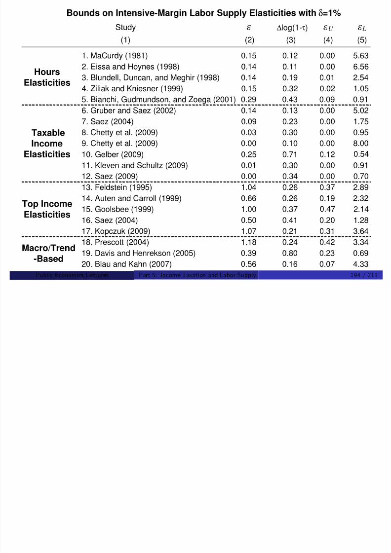
8/8/2019 Chetty - Public Economics Lectures
http://slidepdf.com/reader/full/chetty-public-economics-lectures 589/949
Percentage Change in Net of Tax Rate ∆ log (1 – τ)
0.0
0.5
1.0
1.5
0.2 0.3 0.4 0.5 0.6 0.7 0.8
Source: Chetty 2009
Public Economics Lectures ()Part 5: Income Taxation and Labor Supply 195 / 211
Bounds on Intensive-Margin Labor Supply Elasticities with δ=1%
E l a s t i c i t y
2.0
2.5
3.0
3.5
4.0
No disjoint sets: δ=1% reconciles all estimates
Feldstein (1995)
Kopczuk (2009)
Prescott (2004)
Goolsbee (1999)
Auten and Carroll (1999)
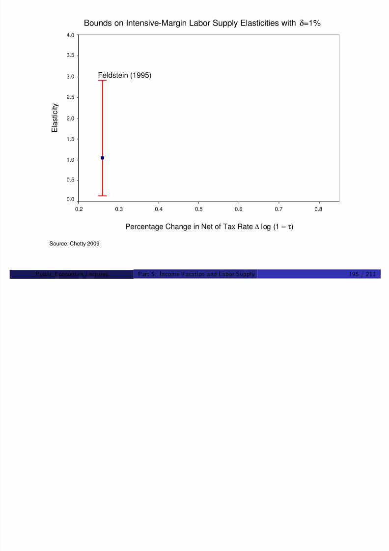
8/8/2019 Chetty - Public Economics Lectures
http://slidepdf.com/reader/full/chetty-public-economics-lectures 590/949
Percentage Change in Net of Tax Rate ∆ log (1 – τ)
0.0
0.5
1.0
1.5
0.2 0.3 0.4 0.5 0.6 0.7 0.8
Saez (2004)
Bianchi et al. (2001)
Gelber (2009)
Davis and Hen-rekson (2005)
Source: Chetty 2009
Public Economics Lectures ()Part 5: Income Taxation and Labor Supply 196 / 211
Bounds on Intensive-Margin Labor Supply Elasticities with δ=1%
E l a s t i c i t y
2.0
2.5
3.0
3.5
4.0
Feldstein (1995)
Kopczuk (2009)
Prescott (2004)
Goolsbee (1999)
S (2004) D i d H
Auten and Carroll (1999)
Unified Bounds: (0.47,0.54)

8/8/2019 Chetty - Public Economics Lectures
http://slidepdf.com/reader/full/chetty-public-economics-lectures 591/949
Percentage Change in Net of Tax Rate ∆ log (1 – τ)
0.0
0.5
1.0
1.5
0.2 0.3 0.4 0.5 0.6 0.7 0.8
Saez (2004)
Bianchi et al. (2001)
Gelber (2009)
Davis and Hen-rekson (2005)
Source: Chetty 2009
Public Economics Lectures ()Part 5: Income Taxation and Labor Supply 197 / 211
Information and Salience in Income Taxation
Recent evidence indicates that one important “friction” isinformation/salience.
Confusion between average and marginal tax rates: de Bartolome

8/8/2019 Chetty - Public Economics Lectures
http://slidepdf.com/reader/full/chetty-public-economics-lectures 592/949
g g(1996), Liebman and Zeckhauser (2004)
Evidence that information a¤ects behavioral responses to incometaxes: Chetty and Saez (2008)
Public Economics Lectures ()Part 5: Income Taxation and Labor Supply 198 / 211
Chetty and Saez 2009: Experimental Design
119 H&R Block o¢ces in Chicago metro area; 43,000 EITC clients
1,461 tax professionals implemented experiment
Tax Season 2007: Jan. 1 to April 15, 2007
8/8/2019 Chetty - Public Economics Lectures
http://slidepdf.com/reader/full/chetty-public-economics-lectures 593/949
EITC clients randomly assigned to control or treatment group
Control group: standard tax preparation procedure
Only mentions the EITC amount, with no info on EITC structure
Public Economics Lectures ()Part 5: Income Taxation and Labor Supply 199 / 211

8/8/2019 Chetty - Public Economics Lectures
http://slidepdf.com/reader/full/chetty-public-economics-lectures 594/949
Public Economics Lectures ()Part 5: Income Taxation and Labor Supply 200 / 211
Year 2 Earnings Distributions: 1 Dep., Clients of Complying Tax Preparers
0 0
3 0 0 0 4
0 0 0
5 0 0 0
6 0 0 0
a r n i n g s D e n
s i t y
E I T C
A m o u n
t ( $ )
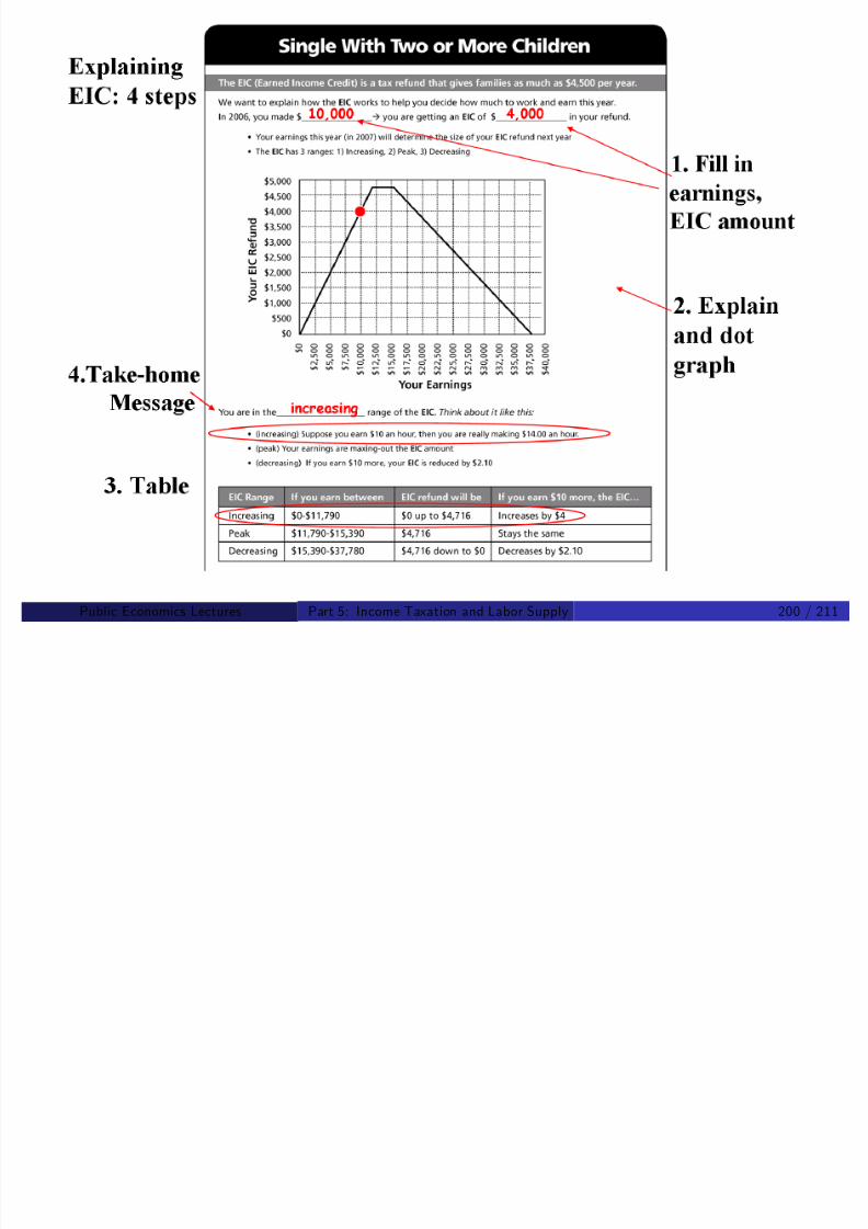
8/8/2019 Chetty - Public Economics Lectures
http://slidepdf.com/reader/full/chetty-public-economics-lectures 595/949
0
1 0 0
0
2 0 0
0 5000 10000 15000 20000 25000 30000 35000 40000
E a
E
Post-Treatment (Year 2) Earnings ($)
Control Treatment EITC Amount
Post-Treatment (Year 2) Earnings ($)
Control Treatment EITC Amount
Source: Chetty and Saez 2009
Public Economics Lectures ()Part 5: Income Taxation and Labor Supply 201 / 211
Self-Employed Clients of Complying Tax Professionals: 1 Dependent
E a r n i n g s D e n
s i t y
E I T C
A m o u n
t ( $ )
0 0 0
4
0 0 0
6 0 0 0
3 0 0 0
5 0 0 0

8/8/2019 Chetty - Public Economics Lectures
http://slidepdf.com/reader/full/chetty-public-economics-lectures 596/949
Post-Treatment (Year 2) Earnings ($)
Control Treatment EITC Amount
Post-Treatment (Year 2) Earnings ($)
Control Treatment EITC Amount
E
0
0 5000 10000 15000 20000 25000 30000 35000 40000
E 2 0
1 0 0
0
Source: Chetty and Saez 2009
Public Economics Lectures ()Part 5: Income Taxation and Labor Supply 202 / 211
Year 2 Wage Earnings Distributions: Complying Tax Preparers, 1 Dependent
0 0
3 0 0 0 4
0 0 0
5 0 0 0
6 0 0 0
E a r n i n g s D e n
s i t y
E I T C
A m o u n
t ( $ )

8/8/2019 Chetty - Public Economics Lectures
http://slidepdf.com/reader/full/chetty-public-economics-lectures 597/949
0
1 0 0
0
2 0
0 5000 10000 15000 20000 25000 30000 35000 40000
E E
Control Treatment EITC Amount
Post-Treatment (Year 2) Wage Earnings ($)
Source: Chetty and Saez 2009
Public Economics Lectures ()Part 5: Income Taxation and Labor Supply 203 / 211
Calibration: Magnitude of Information E¤ects
How big is the behavioral response to the information relative to
e¤ects of conventional policy instruments?
Existing literature implies intensive margin elasticity of earnings w.r.t.1-MTR of at most ε = 0 25
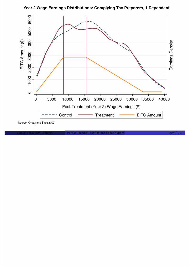
8/8/2019 Chetty - Public Economics Lectures
http://slidepdf.com/reader/full/chetty-public-economics-lectures 598/949
1-MTR of at most ε = 0.25
Complying tax pros increase treated clients’ EITC by $58
EITC expansion of 33 percent would generate same response
Public Economics Lectures ()Part 5: Income Taxation and Labor Supply 204 / 211
Labor Supply Elasticities: Implications for Preferences
Labor supply elasticities central for tax policy because they determinee¢ciency costs
But optimal income tax policy also depends on bene…ts of redistribution (curvature of utility fn.)
u (c ) ψ(l )

8/8/2019 Chetty - Public Economics Lectures
http://slidepdf.com/reader/full/chetty-public-economics-lectures 599/949
Curvature of u (c ): γ = u cc
u c c determines how much more low
income individuals value $1 relative to higher income individuals
Risk aversion parameter γ also central for social insurance literatureand macro models
Evidence on labor supply elasticities also contains information aboutγ (King, Plosser, Rebelo 1988; Basu and Kimball 2002; Chetty 2006)
Public Economics Lectures ()Part 5: Income Taxation and Labor Supply 205 / 211
Chetty 2006
Suppose marginal utility of consumption declines quickly, i.e. γ large
Then as wages rise, individuals should quickly become sated withgoods
Therefore, they should opt to consume much more leisure whenwages rise
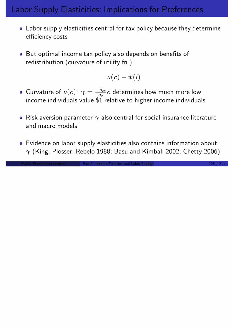
8/8/2019 Chetty - Public Economics Lectures
http://slidepdf.com/reader/full/chetty-public-economics-lectures 600/949
But this would imply εl ,w << 0
Ex: if marginal utility of consumption drops to zero, agent reduces
labor supply 1-1 as wage rises
But we know that increases in wages do not cause sharp reductions in
labor supply (εl ,w > 0.1)
Places an upper bound on size of γ
Public Economics Lectures ()Part 5: Income Taxation and Labor Supply 206 / 211
Chetty: Formula for Risk Aversion
Let y = unearned inc, w = wage, l = labor supply and u (c , l ) =utility
At an interior optimum, l must satisfy
wu c (y + wl , l ) = u l (y + wl , l ) (1)
Work until point where marginal utility of an additional dollar is o¤set

8/8/2019 Chetty - Public Economics Lectures
http://slidepdf.com/reader/full/chetty-public-economics-lectures 601/949
p g yby marginal disutility of work required to earn that dollar
Comparative statics of this condition implies (if u cl = 0):
γ = (1 +wl
y )εl ,y
εl c ,w
Risk aversion directly related to ratio of income e¤ect to substitutione¤ect
Public Economics Lectures ()Part 5: Income Taxation and Labor Supply 207 / 211
Chetty 2006: Graphical Intuition
Assume y = 0. At initial wage w 0, agent works l 0 hours
Consider e¤ect of increasing w by 1% to w 1
Shifts wu c curve up by 1% (substitution e¤ect)
Shifts wu c curve down by ∂ log u c
∂ log w = γ% because γ is elasticity of MU
w.r.t. c (income e¤ect)

8/8/2019 Chetty - Public Economics Lectures
http://slidepdf.com/reader/full/chetty-public-economics-lectures 602/949
Therefore, γ < 1 () εl ,w > 0
If u cl 6= 0, then u l curve shifts when w changes
But the shift is u l
relatively small, so change in l can still be usedto get a bound on γ
Public Economics Lectures ()Part 5: Income Taxation and Labor Supply 208 / 211
w0uc(w0l,l)-u
l(w0l,l)
uc ,ul
w1uc(w1l,l)
Case B: γ > 1
-ul range with
complementarity
Case A: γ < 1
w1uc(w1l,l)

8/8/2019 Chetty - Public Economics Lectures
http://slidepdf.com/reader/full/chetty-public-economics-lectures 603/949
llB l0 lA
Source: Chetty 2006
Public Economics Lectures ()Part 5: Income Taxation and Labor Supply 209 / 211
Labor Supply Elasticities and Implied Coefficients of Relative Risk Aversion
Income Compensated γ γ
Study Sample Identification Elasticity Wage Elasticity Addit ive ∆c/c=0.15
(1) (2) (3) (4) (5) (6) (7)
A. Hours
MaCurdy (1981) Married Men Panel -0.020 0.130 0.46 0.60
Blundell and MaCurdy (1999) Men Various -0.120 0.567 0.63 0.82
MaCurdy, Green, Paarsch (1990) Married Men Cross Section -0.010 0.035 1.47 1.81
Eissa and Hoynes (1998) Married Men, Inc < 30K EITC Expansions -0.030 0.192 0.88 1.08
Married Women, Inc < 30K EITC Expansions -0.040 0.088 0.64 1.34
Friedberg (2000) Older Men (63-71) Soc. Sec. Earnings Test -0.297 0.545 0.93 1.46
Blundell, Duncan, Meghir (1998) Women, UK Tax Reforms -0.185 0.301 0.93 1.66
Average 0.69 0.94
B. Participation
Eissa and Hoynes (1998) Married Men, Inc < 30K EITC Expansions -0.008 0.033 0.44 0.48
Married Women, Inc < 30K EITC Expansions -0.038 0.288 0.15 0.30
A erage 0 29 0 39

8/8/2019 Chetty - Public Economics Lectures
http://slidepdf.com/reader/full/chetty-public-economics-lectures 604/949
Average 0.29 0.39
C. Earned Income
Imbens, Rubin, Sacerdote (2001) Lottery Players in MA Lottery Winnings -0.110Feldstein (1995) Married, Inc > 30K TRA 1986 1.040 0.32 0.41
Auten and Carroll (1997) Single and Married, Inc>15K TRA 1986 0.660 0.50 0.65
Average 0.41 0.53
D. Macroeconomic/Trend Evidence
Blau and Kahn (2005) Women Cohort Trends -0.278 0.646 0.60 1.29
Davis and Henrekson (2004) Europe/US aggregate stats Cross-Section of countries -0.251 0.432 1.74 2.25
Prescott (2004) Europe/US aggregate stats Cross-Country time series -0.222 0.375 1.78 2.30
Average 1.37 1.95
Overall Average 0.71 0.97
Source: Chetty 2006
Public Economics Lectures ()Part 5: Income Taxation and Labor Supply 210 / 211
Chetty 2006: Results
Labor supply evidence justi…es use of u (c ) = log c
Formula γ = (1 + wl y
)εl ,y
εl cuseful in tax, insurance, and other
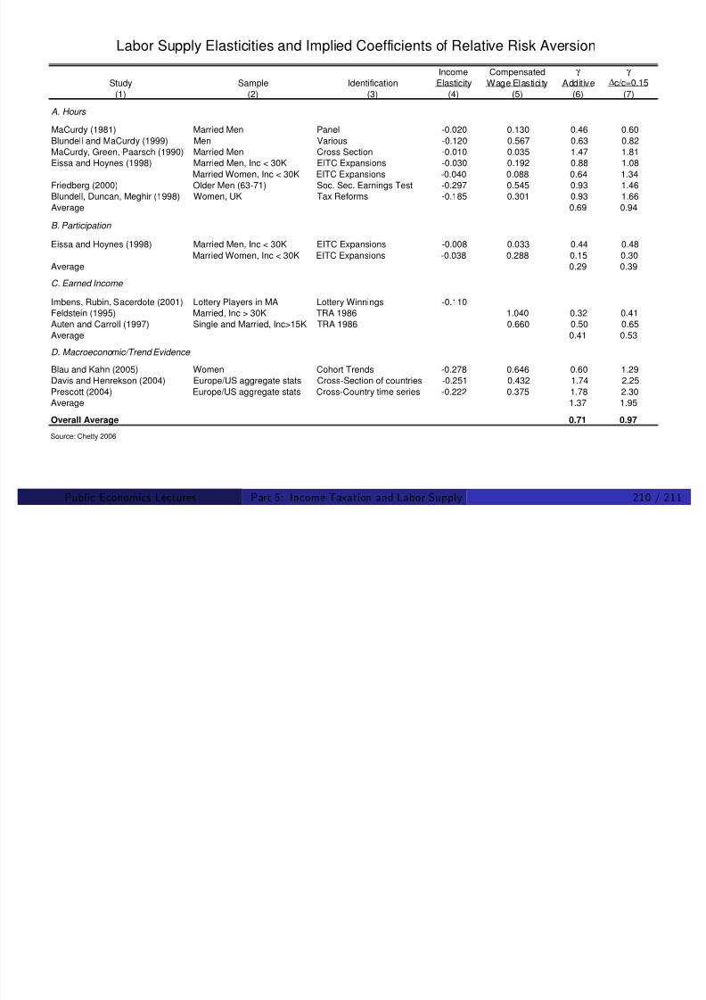
8/8/2019 Chetty - Public Economics Lectures
http://slidepdf.com/reader/full/chetty-public-economics-lectures 605/949
γ (y
) εl c ,w
applications
Public Economics Lectures ()Part 5: Income Taxation and Labor Supply 211 / 211
Public Economics Lectures
Part 6: Social Insurance
Raj Chetty and Gregory A. Bruich

8/8/2019 Chetty - Public Economics Lectures
http://slidepdf.com/reader/full/chetty-public-economics-lectures 606/949
Harvard UniversityFall 2009
Public Econom ics Lectures () Part 6: Social Insurance 1 / 207
Outline
1 Motivations for Social Insurance
2 Unemployment Insurance
3 Workers’ Compensation

8/8/2019 Chetty - Public Economics Lectures
http://slidepdf.com/reader/full/chetty-public-economics-lectures 607/949
p
4 Disability Insurance
5 Health Insurance
Public Econom ics Lectures () Part 6: Social Insurance 2 / 207
De…nition of Social Insurance
Transfers based on events such as unemployment, disability, or age
Contrasts with welfare: means-tested transfers

8/8/2019 Chetty - Public Economics Lectures
http://slidepdf.com/reader/full/chetty-public-economics-lectures 608/949
SI is the biggest and most rapidly growing part of governmentexpenditure today
Public Econom ics Lectures () Part 6: Social Insurance 3 / 207
Growth of Social Insurance in the U.S.
National Defense
NationalDefense20.7%
Other
21.6%
IncomeSecurity
5%
SocialSecurity20.7%
Social
Security3.6%
Health
9.4%
Health0.4%

8/8/2019 Chetty - Public Economics Lectures
http://slidepdf.com/reader/full/chetty-public-economics-lectures 609/949
National Defense
69.4% Other34.8%
Income
Security14.5%
1953 2008
Source: Office of Management and Budget, historical tables, government outlays by function
Public Econom ics Lectures () Part 6: Social Insurance 4 / 207

8/8/2019 Chetty - Public Economics Lectures
http://slidepdf.com/reader/full/chetty-public-economics-lectures 610/949
t r e p l a c e m e n t r
a t e ( % )
4 0
6 0
8 0
1 0 0
1 2 0
Unemployment Benefit Systems in Developed Countries

8/8/2019 Chetty - Public Economics Lectures
http://slidepdf.com/reader/full/chetty-public-economics-lectures 611/949
N e t
0
2 0
Time (months)
0 5 10 15 20 25 30 35 40 45 50 55 60
Source: OECD Benefits and Wages 2002
SwedenSwedenHungaryHungary SpainSpainBelgiumBelgium USAUSA
Public Econom ics Lectures () Part 6: Social Insurance 6 / 207
Main Questions in Social Insurance
1 Why have social (as opposed to private, or any) insurance?
2 What type of SI system maximizes social welfare?
Tradeo¤ between two forces:
Bene…ts – reducing risk (‡uctuations in consumption)Distortion – changes in incentives for workers and …rms –> ine¢cient
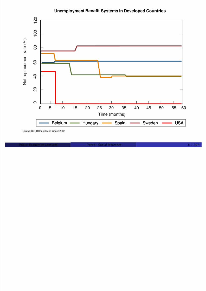
8/8/2019 Chetty - Public Economics Lectures
http://slidepdf.com/reader/full/chetty-public-economics-lectures 612/949
Distortion changes in incentives for workers and …rms > ine¢cient
behavior and DWL
Generate new distortions as you …x the problem you set out to solve–> second-best solution
Identify optimal policy by combining theoretical models of socialinsurance with empirical evidence on program e¤ects
Public Econom ics Lectures () Part 6: Social Insurance 7 / 207
Useful Background Reading
1 Institutional details: see handout posted on course website
2 Expected utility theory: See MWG or other graduate texts
3 Empirical program evaluation methods: Du‡o handout on website

8/8/2019 Chetty - Public Economics Lectures
http://slidepdf.com/reader/full/chetty-public-economics-lectures 613/949
4 Survival analysis: Kiefer (1988 JEL)
5 Surveys: Krueger and Meyer Handbook 2002 (empirics), Chetty AnnRev. 2009 (theory)
Public Econom ics Lectures () Part 6: Social Insurance 8 / 207
Why have social insurance?
Motivation for insurance: reduction in risk for risk-averse individuals
Unemp Ins: risk of involuntary unemployment
Workers’ comp and DI: risk of injuries/disabilitiesSocial Security annuity: risk of living too long
But why is government intervention needed to provide this?

8/8/2019 Chetty - Public Economics Lectures
http://slidepdf.com/reader/full/chetty-public-economics-lectures 614/949
insurance?
Possible sources of market failure here:
1 Informational problems (adverse selection)
2 Individual optimization failures (myopia/improper planning)3 Macroeconomic shocks
Public Econom ics Lectures () Part 6: Social Insurance 9 / 207
Adverse Selection as a Motivation for SI
Key paper: Rothschild and Stiglitz (1976); see MWG Ch. 13 for agood review
Consider an environment with asymmetric information, e.g.individuals know risk of losing job but insurer does not

8/8/2019 Chetty - Public Economics Lectures
http://slidepdf.com/reader/full/chetty-public-economics-lectures 615/949
Main result: can lead to market failure where no equilibrium supportsprovision of insurance
Government intervention through mandated insurance can increasewelfare
Public Econom ics Lectures () Part 6: Social Insurance 10 / 207
Rothschild-Stiglitz model
Economy with two types, low-risk (L) and high-risk (H)
A fraction f of the individuals are high-risk
Type L has a chance p L of becoming unemployed in a given year

8/8/2019 Chetty - Public Economics Lectures
http://slidepdf.com/reader/full/chetty-public-economics-lectures 616/949
Type H has a chance p H > p L of becoming unemployed.
In good state (state 1), income is E 1 for both types; in bad state,income is E 2 < E 1.
Public Econom ics Lectures () Part 6: Social Insurance 11 / 207
Rothschild-Stiglitz: Key Assumptions
1 Static model: individuals arrive in the period either employed or
unemployed; no savings/dynamics.
2 No moral hazard: agents choose insurance contract but make nochoices after signing a contract.
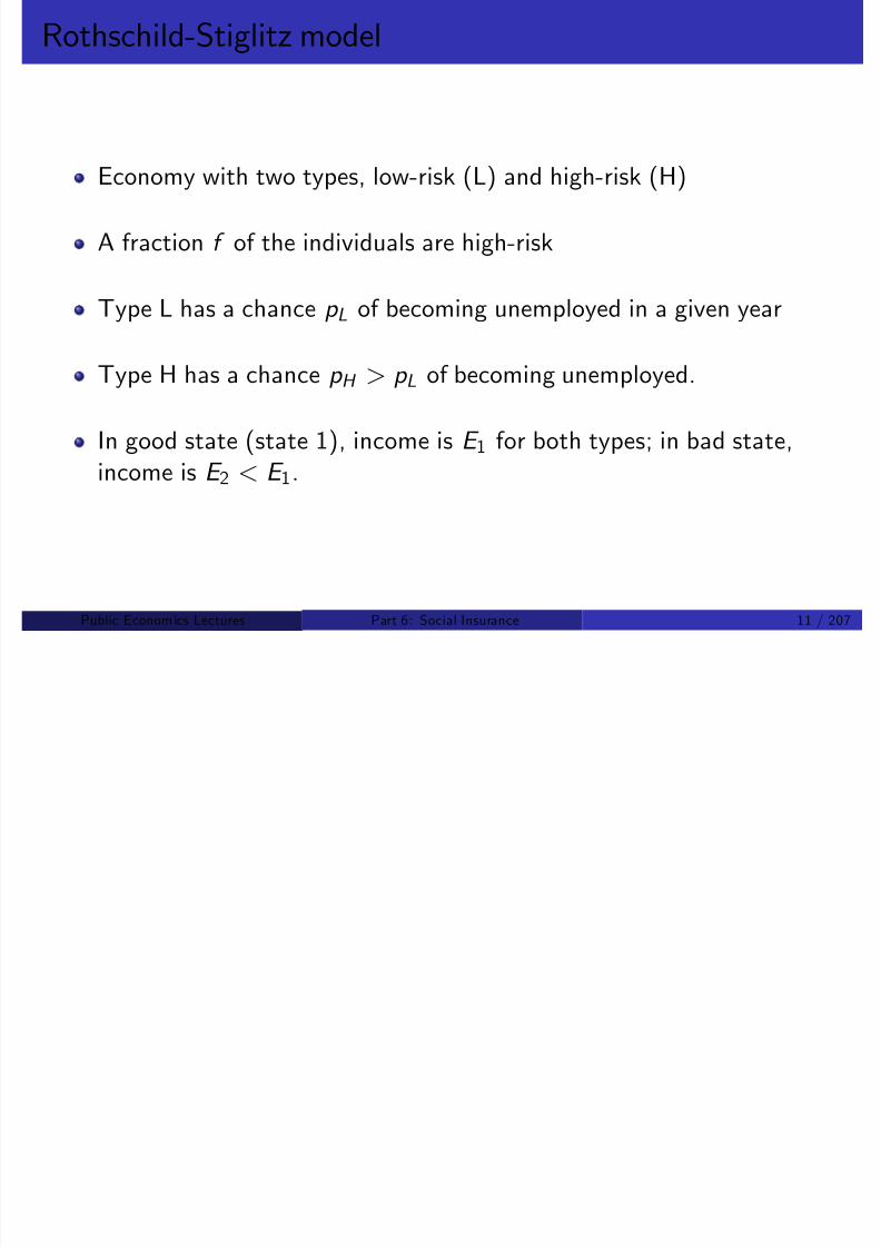
8/8/2019 Chetty - Public Economics Lectures
http://slidepdf.com/reader/full/chetty-public-economics-lectures 617/949
3 Insurance market is perfectly competitive, so …rms earn zero pro…tsin equilibrium.
Public Econom ics Lectures () Part 6: Social Insurance 12 / 207
Rothschild-Stiglitz: Contracts
An insurance contract is described by a vector α = (α1, α2)
Consumption in the two states: (E 1 α1, E 2 + α2)
Type i ’s expected utility is
V i (α) = (1 p i )u (E 1 α1) + p i u (E 2 + α2)

8/8/2019 Chetty - Public Economics Lectures
http://slidepdf.com/reader/full/chetty-public-economics-lectures 618/949
Any contract that earns non-negative pro…ts is feasible
Zero-pro…t condition ) …rms price insurance s.t.
α2 =1 p
p
α1
where p is risk rate of those who purchase contract.
Public Econom ics Lectures () Part 6: Social Insurance 13 / 207
Rothschild-Stiglitz: Equilibrium
De…nition
An equilibrium is de…ned by a set of insurance contracts such that(1) individuals optimize: both types cannot …nd a better contract than the
ones they chose(2) …rms optimize: all …rms earn zero pro…ts
Two types of equilibrium:

8/8/2019 Chetty - Public Economics Lectures
http://slidepdf.com/reader/full/chetty-public-economics-lectures 619/949
Two types of equilibrium:
1 Pooling: both types are o¤ered the same contract α.
2 Separating: high-risk types choose a contract αH while low-risk typeschoose a di¤erent contract αL.
Public Econom ics Lectures () Part 6: Social Insurance 14 / 207
Rothschild-Stiglitz: First Best Solution
In …rst best, insurer can distinguish types (perfect information)
In this case, equilibrium is separating
Plugging in α2 = 1p i p i
α1, each type solves
maxα1
(1 p i )u (w α1) + p i u (w +1 p i
p i α1).

8/8/2019 Chetty - Public Economics Lectures
http://slidepdf.com/reader/full/chetty-public-economics-lectures 620/949
Solution
Set MRS 12 = 1p i p i
, i.e. u 0(c 1) = u 0(c 2), i.e. full insurance
Both types are perfectly insured: earn their expected income(1 p i )w regardless of the state.
Public Econom ics Lectures () Part 6: Social Insurance 15 / 207

8/8/2019 Chetty - Public Economics Lectures
http://slidepdf.com/reader/full/chetty-public-economics-lectures 621/949
Public Econom ics Lectures () Part 6: Social Insurance 16 / 207
Rothschild-Stiglitz: Second Best Problem
Firms cannot distinguish types in practice, because they cannotdetermine true layo¤ risks, illness history, etc.
With contracts above, all the high risk types buy the low risk’scontract and insurer goes out of business

8/8/2019 Chetty - Public Economics Lectures
http://slidepdf.com/reader/full/chetty-public-economics-lectures 622/949
Hence optimal contracts di¤er when information is asymmetric
Public Econom ics Lectures () Part 6: Social Insurance 17 / 207
Rothschild-Stiglitz: Second Best Solution
Result #1: no pooling equilibrium exists
If H and L types are pooled in a contract α,low-risk types lose moneyin expectation.
Zero-pro…t condition requires α2 = 1p p
α1 but p > p L.
Low-risk type gets fewer dollars in state 2 than he should if the

8/8/2019 Chetty - Public Economics Lectures
http://slidepdf.com/reader/full/chetty-public-economics-lectures 623/949
insurance were fair for him.
Creates an opportunity for a new insurer to enter and “pick o¤” lowrisk types by o¤ering slightly less insurance at a better price: higherc 1, lower c 2
Only low risk types switch, because they value c 1 more.
Public Econom ics Lectures () Part 6: Social Insurance 18 / 207

8/8/2019 Chetty - Public Economics Lectures
http://slidepdf.com/reader/full/chetty-public-economics-lectures 624/949
Public Econom ics Lectures () Part 6: Social Insurance 19 / 207
Rothschild-Stiglitz: Second Best Solution
Result #2: in a separating eq, Type H obtains full insurance andType L is under-insured
Intuition: in any sep. eq., both types are getting actuarially fair
insurance because of the zero-pro…ts condition
For H, no cost to …rm in providing full ins. (worst that can happen isthat L will join the pool, raising pro…ts)
But for L full ins would create an incentive for H to buy this

8/8/2019 Chetty - Public Economics Lectures
http://slidepdf.com/reader/full/chetty-public-economics-lectures 625/949
But for L, full ins. would create an incentive for H to buy this(cheaper) policy, forcing …rm into negative pro…ts
Incentive constraints always bind downward – “no distortion at thetop” result in standard asymmetric info. models
In eq., L gets as much ins as possible without inducing H to deviateand pretend to be low-risk
Public Econom ics Lectures () Part 6: Social Insurance 20 / 207
Rothschild-Stiglitz: Gains from Government Mandate
There can be gains from government intervention through mandatedinsurance
Consider an example where
E 1 = 100, E 2 = 0
u (c ) =p
c , p L =1
4, p H =
3
4, f = 10%

8/8/2019 Chetty - Public Economics Lectures
http://slidepdf.com/reader/full/chetty-public-economics-lectures 626/949
4 4
In candidate separating eq., type H gets perfect insurance:
EU H = u (100(1
p H )) = r 100
1
4
= 5
Public Econom ics Lectures () Part 6: Social Insurance 21 / 207
Rothschild-Stiglitz: Second Best Solution
Type L gets as much ins. as possible without making H want todeviate at actuarially fair rate for L:
5 = 14
q 100 αL
1 + 34
s 1 p L
p LαL
1
Solving gives αL1 = $3.85, αL
2 = $11.55 – nowhere near full insurancefor low risk type

8/8/2019 Chetty - Public Economics Lectures
http://slidepdf.com/reader/full/chetty-public-economics-lectures 627/949
for low risk type.
Note that expected utility for low risk type is
EU L =3
4
p 100
3.85 +
1
4
p 3
3.85 = 8.2.
Public Econom ics Lectures () Part 6: Social Insurance 22 / 207
Rothschild-Stiglitz: Second Best Solution
Now suppose govt. comes in and mandates pooled insurance atactuarial rate. Everyone gets an income of
(9
10
3
4+
1
10
1
4)100 =
7
10100 = 70.

8/8/2019 Chetty - Public Economics Lectures
http://slidepdf.com/reader/full/chetty-public-economics-lectures 628/949
H bene…ts from this: now pooling with less risky people
But L bene…ts too! Expected utility isp
70 > 8.2
Public Econom ics Lectures () Part 6: Social Insurance 23 / 207
Rothschild-Stiglitz: Second Best Solution
Because there are relatively few high risk types, L types bene…t frompooling with them and getting full insurance coverage.
Note: pooled contract of 70 could be o¤ered by a private …rm,destroying separating eq. proposed above

8/8/2019 Chetty - Public Economics Lectures
http://slidepdf.com/reader/full/chetty-public-economics-lectures 629/949
Hence there is actually no equilibrium in this example
Public Econom ics Lectures () Part 6: Social Insurance 24 / 207
Adverse Selection as a Motivation for SI
More generally, consider an economy in which people di¤er in theirrisks of becoming unemployed
Adverse selection can destabilize the market:Firm provides UI but lowest-risk (tenured people) drop out ) rateshave to riseBut then even moderate-risk types opt out ) rates rise further, moredrop out, ...

8/8/2019 Chetty - Public Economics Lectures
http://slidepdf.com/reader/full/chetty-public-economics-lectures 630/949
Could cause unraveling to the point where virtually no one is insured byprivate marketUI program that pools everyone can lead to (ex-ante) welfareimprovements
What tool does the govt. have that private sector does not? Abilityto mandate
Public Econom ics Lectures () Part 6: Social Insurance 25 / 207
Adverse Selection: Empirical Evidence
Empirical evidence shows that adverse selection is a real source of market failures in practice
General test: “positive correlation” property in equilibrium
Are those who buy more insurance more likely to …le claims?
Could be driven by both moral hazard + AS but not in certain contexts

8/8/2019 Chetty - Public Economics Lectures
http://slidepdf.com/reader/full/chetty-public-economics-lectures 631/949
such as death
Example: Finkelstein and Poterba (2004): adverse selection in U.K.annuity market.
Annuities = ins. against the risk of living too long.
Public Econom ics Lectures () Part 6: Social Insurance 26 / 207
Finkelstein and Poterba 2004
Study two types of annuity markets: compulsory vs. voluntary.
Examine two features of annuity contracts
degree of backloading (in‡ation indexing and escalation of paymentsover time)payments to estate in event of death (guarantees and capitalprotection).
Test for positive correlation in two ways

8/8/2019 Chetty - Public Economics Lectures
http://slidepdf.com/reader/full/chetty-public-economics-lectures 632/949
Test for positive correlation in two ways
1 In eq., those who purchase backloaded annuities have lower mortalityrates
2 In eq., those who purchase annuities with payment to estate havehigher mortality rates
Both e¤ects should be stronger in voluntary markets
Public Econom ics Lectures () Part 6: Social Insurance 27 / 207

8/8/2019 Chetty - Public Economics Lectures
http://slidepdf.com/reader/full/chetty-public-economics-lectures 633/949
Public Econom ics Lectures () Part 6: Social Insurance 28 / 207
Individual Optimization Failures as a Motivation for SI
Given adverse selection, expect individuals to “self-insure” againsttemp. shocks by building up savings
With such bu¤er stocks, still no need for large social safety nets to
insure against temporary shocks such as unemployment
In practice, individuals appear to be very liquidity constrained whenhit by shocks: median job loser has <$200 in assets

8/8/2019 Chetty - Public Economics Lectures
http://slidepdf.com/reader/full/chetty-public-economics-lectures 634/949
Suggests 1st Welfare thm also does not hold due to individual failuresto optimize
Individuals may misperceive the probability of a layo¤
Firms may not be able to debias people in equilibrium, leading to rolefor govt. (Spinnewijn 2009)
Public Econom ics Lectures () Part 6: Social Insurance 29 / 207
Aggregate Shocks as a Motivation for SI
Private ins. (cross-sectional pooling) relies on idiosyncratic risks sothose who are well o¤ can pay those who are poor
Government is the only entity able to coordinate risk-sharing acrossdi¤erent groups that are all a¤ected by negative shocks
Inter-generational risk sharing required if everyone is poor at the same

8/8/2019 Chetty - Public Economics Lectures
http://slidepdf.com/reader/full/chetty-public-economics-lectures 635/949
time
Particularly relevant for UI and maybe social security
Less so for health-related shocks
Public Econom ics Lectures () Part 6: Social Insurance 30 / 207
Optimal Social Insurance
Now turn to question of optimal design of SI policies
Take as given that market provides no insurance for some reason
In the simple Rothschild-Stiglitz model, perfect insurance is optimal
But this abstracts from the central moral hazard problem

8/8/2019 Chetty - Public Economics Lectures
http://slidepdf.com/reader/full/chetty-public-economics-lectures 636/949
Individuals will not work if they have perfect unemp insurance
Must take this distortion into account to …nd optimal level of socialinsurance
Public Econom ics Lectures () Part 6: Social Insurance 31 / 207
Unemployment Insurance
Start with UI: approx. $40 bn/yr. paid to people who get laid o¤
Potential bene…ts
1 Smoother path of consumption
2 Better job matches

8/8/2019 Chetty - Public Economics Lectures
http://slidepdf.com/reader/full/chetty-public-economics-lectures 637/949
Potential distortions:
1 Less job search, higher unemployment rate
2 Workers’ preferences distorted toward unstable jobs
3 Shirking because fear of job loss not as great
4 Less savings
Public Econom ics Lectures () Part 6: Social Insurance 32 / 207
Optimal UI: Outline
1 Optimal level of UI bene…ts ignoring …rm responses [Baily-Chettymodel]
Theory applies to all the income security programs discussed later
2 Distortions to …rms’ layo¤ decisions due to imperfect exp rating

8/8/2019 Chetty - Public Economics Lectures
http://slidepdf.com/reader/full/chetty-public-economics-lectures 638/949
[Feldstein model]
3 Other issues: Post-unemployment outcomes, general equilibriume¤ects
Public Econom ics Lectures () Part 6: Social Insurance 33 / 207
Replacement Rate
Common measure of program’s size is its “replacement rate”
r =net bene…t
net wage
UI reduces agents’ e¤ective wage rate from …nding a new job tow (1 r )
Feldstein (1978): UI makes e¤ective wages very low because of interaction with tax system:

8/8/2019 Chetty - Public Economics Lectures
http://slidepdf.com/reader/full/chetty-public-economics-lectures 639/949
1970: No tax ) r = (0.5)w (1.18.05.07)w
= 72%
Incentives worse for some subgroups: secondary income earner facesMTR of 50% ) r = 1.3
Today, federal income taxes paid on UI bene…ts, so rep. rate is50-60%
Public Econom ics Lectures () Part 6: Social Insurance 34 / 207

8/8/2019 Chetty - Public Economics Lectures
http://slidepdf.com/reader/full/chetty-public-economics-lectures 640/949
Baily-Chetty model
Canonical analysis of optimal level of UI bene…ts: Baily (1978)
Shows that the optimal bene…t level can be expressed as a fn of a
small set of parameters in a static model.
Once viewed as being of limited practical relevance because of strongassumptions
C ( )
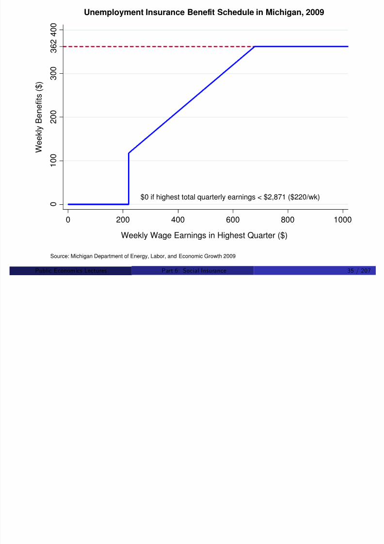
8/8/2019 Chetty - Public Economics Lectures
http://slidepdf.com/reader/full/chetty-public-economics-lectures 641/949
Chetty (2006) shows formula actually applies with arbitrary choicevariables and constraints.
Parameters identi…ed by Baily are su¢cient statistics for welfare
analysis ) robust yet simple guide for optimal policy.
Public Econom ics Lectures () Part 6: Social Insurance 36 / 207
Baily-Chetty model: Assumptions
1
Fixed wages – no GE e¤ects
2 No distortions to …rm behavior (temporary layo¤s); implicitly assumeperfect experience rating
3 N li i h ill h

8/8/2019 Chetty - Public Economics Lectures
http://slidepdf.com/reader/full/chetty-public-economics-lectures 642/949
3 No externalities such as spillovers to search
Public Econom ics Lectures () Part 6: Social Insurance 37 / 207
Baily-Chetty model: Setup
Static model with two states: high (employed) and low (unemployed)
Let w h denote the individual’s income in the high state and w l < w h
income in the low state
Let A denote wealth, c h consumption in the high state, and c l consumption in the low state
A t i i iti ll l d C t l b bilit f b i i th b d
8/8/2019 Chetty - Public Economics Lectures
http://slidepdf.com/reader/full/chetty-public-economics-lectures 643/949
Agent is initially unemployed. Controls probability of being in the badstate by exerting search e¤ort e at a cost ψ(e )
Choose units of e so that the probability of being in the high state is
given by p (e ) = e
Public Econom ics Lectures () Part 6: Social Insurance 38 / 207
Baily-Chetty model: Setup
UI system that pays constant bene…t b to unemployed agents
Bene…ts …nanced by lump sum tax t (b ) in the high state
Govt’s balanced-budget constraint:
e t (b ) = (1 e ) b
L t (c) d t tilit ti ( t i tl )

8/8/2019 Chetty - Public Economics Lectures
http://slidepdf.com/reader/full/chetty-public-economics-lectures 644/949
Let u (c ) denote utility over consumption (strictly concave)
Agent’s expected utility is
eu (A + w h
t (b )) + (1
e )u (A + w l + b )
ψ(e )
Public Econom ics Lectures () Part 6: Social Insurance 39 / 207
Baily-Chetty model: First Best Problem
In …rst best, there is no moral hazard problem
To solve for FB, suppose government chooses b and e joints tomaximize agent’s welfare:
maxb ,e
e (A + w h t ) + (1 e )u (A + w l + b ) ψ(e )
s t t
1 e
e b

8/8/2019 Chetty - Public Economics Lectures
http://slidepdf.com/reader/full/chetty-public-economics-lectures 645/949
s.t. t = e b
Solution to this problem is u 0(c e ) = u 0(c u ) ) full insurance
Public Econom ics Lectures () Part 6: Social Insurance 40 / 207
Baily-Chetty model: Second Best Problem
In second best, cannot eliminate moral hazard problem because e¤ortis unobserved by govt.
Problem: Agents only consider private marginal costs and bene…tswhen choosing e
Social marginal product of work is w private marginal product is w b

8/8/2019 Chetty - Public Economics Lectures
http://slidepdf.com/reader/full/chetty-public-economics-lectures 646/949
Social marginal product of work is w private marginal product is w b
Agents therefore search too little from a social perspective, leading toe¢ciency losses
Public Econom ics Lectures () Part 6: Social Insurance 41 / 207
Baily-Chetty model: Second Best Problem
Agents maximize expected utility, taking b and t (b ) as given
maxe
eu (A + w h
t ) + (1
e )u (A + w l + b )
ψ(e )
Let indirect expected utility be denoted by V (b , t )
Government’s problem is to maximize agent’s expected utility, taking
into account agent’s behavioral responses:

8/8/2019 Chetty - Public Economics Lectures
http://slidepdf.com/reader/full/chetty-public-economics-lectures 647/949
into account agent s behavioral responses:
maxb ,t
V (b , t )
s.t. e (b )t = (1 e (b ))b
Public Econom ics Lectures () Part 6: Social Insurance 42 / 207
Baily-Chetty model: Second Best Problem
Problem
Optimal Social Insurance
maxb
V (b , t (b ))
s.t. e (b )t (b ) = (1 e (b ))b
e (b ) = arg maxe
e u (A + w h t ) + (1 e ) u (A + w l + b ) ψ(e )
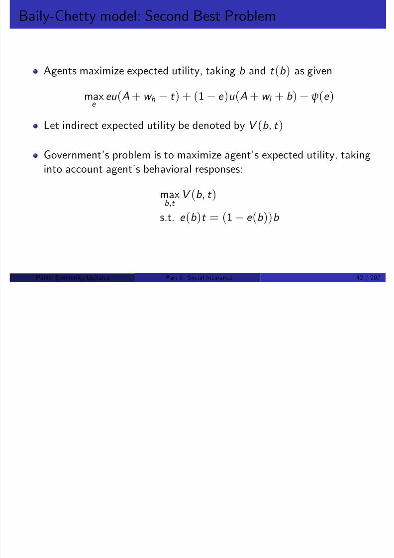
8/8/2019 Chetty - Public Economics Lectures
http://slidepdf.com/reader/full/chetty-public-economics-lectures 648/949
Formally equivalent to an optimal Ramsey tax problem withstate-contingent taxes
Public Econom ics Lectures () Part 6: Social Insurance 43 / 207
Two Approaches to Optimal Social Insurance
1 Structural: specify complete models of economic behavior andestimate the primitives
Identify b as a fn. of discount rates, nature of borrowing constraints,informal ins. arrangements.
Challenge: di¢cult to identify all primitive parameters in an empiricallycompelling manner given unobserved heterogeneity
2 Su¢cient Statistic: derive formulas for b as a fn. of high-level
elasticities
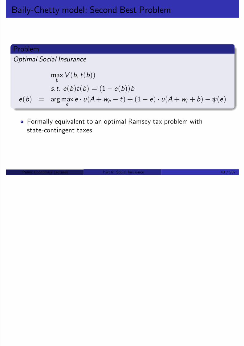
8/8/2019 Chetty - Public Economics Lectures
http://slidepdf.com/reader/full/chetty-public-economics-lectures 649/949
elasticities
These elasticities can be estimated using reduced-form methods
Estimate statistical relationships using quasi-experimental research
designs
Baily-Chetty solution described below is one example
Public Econom ics Lectures () Part 6: Social Insurance 44 / 207
Baily-Chetty model: Second Best Solution
At an interior optimum, the optimal bene…t rate must satisfy
dV /db (b ) = 0
To calculate this derivative, write V (b ) as
V (b ) = maxe
eu (A + w h t (b )) + (1 e )u (A + w l + b ) ψ(e )
Since fn has been optimized over e Envelope Thm implies:

8/8/2019 Chetty - Public Economics Lectures
http://slidepdf.com/reader/full/chetty-public-economics-lectures 650/949
Since fn has been optimized over e , Envelope Thm. implies:dV (b )
db = (1 e )u 0(c l ) dt
db eu 0(c h )
Key: can neglect ∂e
∂b
terms
Public Econom ics Lectures () Part 6: Social Insurance 45 / 207
Envelope Condition
Why can ∂e ∂b
be ignored? Because ∂V ∂e
= 0 by agent optimization.
Contrast with total derivative ignoring optimization of e :
dV (b )db = (1 e )u 0(c l ) dt db
eu 0(c h )
+∂e
∂b [(u (c h ) u (c l ) ψ0(e )]

8/8/2019 Chetty - Public Economics Lectures
http://slidepdf.com/reader/full/chetty-public-economics-lectures 651/949
Second term drops out because f.o.c. for e is
u (c h ) u (c l ) = ψ0(e )
Public Econom ics Lectures () Part 6: Social Insurance 46 / 207
Kaplan 2009
Exploiting f.o.c.’s from agent optimization particularly useful in morecomplex models
Kaplan (2009): unemployed youth move back in with their parents.
How does this a¤ect optimal UI?

8/8/2019 Chetty - Public Economics Lectures
http://slidepdf.com/reader/full/chetty-public-economics-lectures 652/949
Kaplan takes a structural approach and estimates a dynamic model of the decision to move back home
Public Econom ics Lectures () Part 6: Social Insurance 47 / 207
Su¢cient Statistic Approach to Kaplan 2009
Suppose moving home raises consumption by H and has a cost g (H ):
V (b ) = maxe ,H
eu (A + w h t (b ))
+(1
e )[u (A + w l + b + H )
g (H )]
ψ(e )
Variable H drops out, as did e , because of agent optimization
dV (b)

8/8/2019 Chetty - Public Economics Lectures
http://slidepdf.com/reader/full/chetty-public-economics-lectures 653/949
Formula derived fordV (b )
db is una¤ected by ability to move home:
dV (b )
db = (1 e )u 0(c l ) dt
db eu 0(c h )
where c l is measured in the data as including home consumption (H )
Public Econom ics Lectures () Part 6: Social Insurance 48 / 207
Baily-Chetty model: Second Best Solution
The government’s UI budget constraint implies
dt
db =
1 e
e b
e 2de
db =
1 e
e (1 +
ε1e ,b
e )
=) dV (b )db
= (1 e )fu 0(c l ) (1 + ε1e ,b
e )u 0(c h)g
Setting dV (b )/db = 0 yields the optimality condition
u 0(c l ) u 0(c h )0( )= ε1e
,
b

8/8/2019 Chetty - Public Economics Lectures
http://slidepdf.com/reader/full/chetty-public-economics-lectures 654/949
( ) ( )u 0(c h )
εe
LHS: bene…t of transferring $1 from high to low state
RHS: cost of transferring $1 due to behavioral responses
Public Econom ics Lectures () Part 6: Social Insurance 49 / 207
Baily-Chetty model: Second Best Solution
u 0(c l ) u 0(c h)
u 0(c h )=
ε1e ,b
e
This equation provides an exact formula for the optimal bene…t rate
Implementation requires identi…cation of u 0(c l )u 0(c h )
u 0(c h )
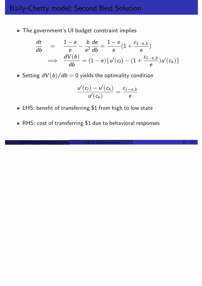
8/8/2019 Chetty - Public Economics Lectures
http://slidepdf.com/reader/full/chetty-public-economics-lectures 655/949
Three ways to identifyu 0(c l )u 0(c h )
u 0(c h )empirically
1 Baily (1978), Gruber (1997), Chetty (2006): cons-based approach2 Shimer and Werning (2007): reservation wages
3 Chetty (2008): moral hazard vs liquidity
Public Econom ics Lectures () Part 6: Social Insurance 50 / 207
Baily-Chetty model: Consumption-Based Formula
Write marginal utility gap using a Taylor expansion
u 0(c l ) u 0(c h ) u 00(c h )(c l c h )
De…ning coe¢cient of relative risk aversion γ = u 00(c )c
u 0(c ), we can write
u 0(c l )
u 0(c h )
u 0(c h ) u 00
u 0 c h
∆c
c (1)

8/8/2019 Chetty - Public Economics Lectures
http://slidepdf.com/reader/full/chetty-public-economics-lectures 656/949
( ) ( )
= γ∆c
c
Gap in marginal utilities is a function of curvature of utility (risk
aversion) and consumption drop from high to low states
Public Econom ics Lectures () Part 6: Social Insurance 51 / 207
Baily-Chetty Consumption-Based Formula
Theorem
The optimal unemployment bene…t level b satis…es
γ∆c
c (b ) ε1
e ,b
e
where
∆c
c
=c h c l
c h= consumption drop during unemployment
00( )

8/8/2019 Chetty - Public Economics Lectures
http://slidepdf.com/reader/full/chetty-public-economics-lectures 657/949
γ = u 00(c h )
u 0(c h )c h = coe¢cient of relative risk aversion
ε1e ,b =d log1 e
d log b = elast. of probability of unemp. w.r.t. bene…ts
Public Econom ics Lectures () Part 6: Social Insurance 52 / 207
Baily-Chetty Consumption-Based Formula
γ∆c
c (b ) ε1e ,b
e
Intuition for formula: LHS is marginal social bene…t of UI, RHS ismarginal social cost of UI
Extends to model where agent chooses N other behaviors and faces M
other constraints, subject to some regularity conditions (Chetty 2006).
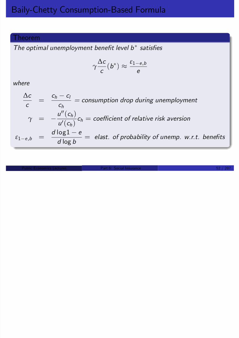
8/8/2019 Chetty - Public Economics Lectures
http://slidepdf.com/reader/full/chetty-public-economics-lectures 658/949
Envelope conditions used above still go through with arbitrary choicevars.
Empirical work on UI can essentially be viewed as providing estimatesof the three key parameters (γ, ∆c
c , ε).
Public Econom ics Lectures () Part 6: Social Insurance 53 / 207
Empirical Estimates: Duration Elasticity
Early literature used cross-sectional variation in replacement rates.
Problem: comparisons of high and low wage earners confounded byother factors.
Modern studies use exogenous variation from policy changes (e.g.Meyer 1990)

8/8/2019 Chetty - Public Economics Lectures
http://slidepdf.com/reader/full/chetty-public-economics-lectures 659/949
(Meyer 1990)
Public Econom ics Lectures () Part 6: Social Insurance 54 / 207
After Benefit Increase
Before Benefit Increase
Weekly
BenefitAmount
WBAmax B
WBAmax A
WBAmin

8/8/2019 Chetty - Public Economics Lectures
http://slidepdf.com/reader/full/chetty-public-economics-lectures 660/949
Previous Earnings
Source: Krueger and Meyer 2002
E 1 E 2 E 3
High Earnings GroupLow Earnings Group
Public Econom ics Lectures () Part 6: Social Insurance 55 / 207
Hazard Models
De…ne hazard rate ht = number that …nd a job at time t divided bynumber unemployed at time t
This is an estimate of the probability of …nding a job at time t
conditional on being unemployed for at least t weeks
Standard speci…cation of hazard model: Cox “proportional hazards”
ht = αt exp( βX )
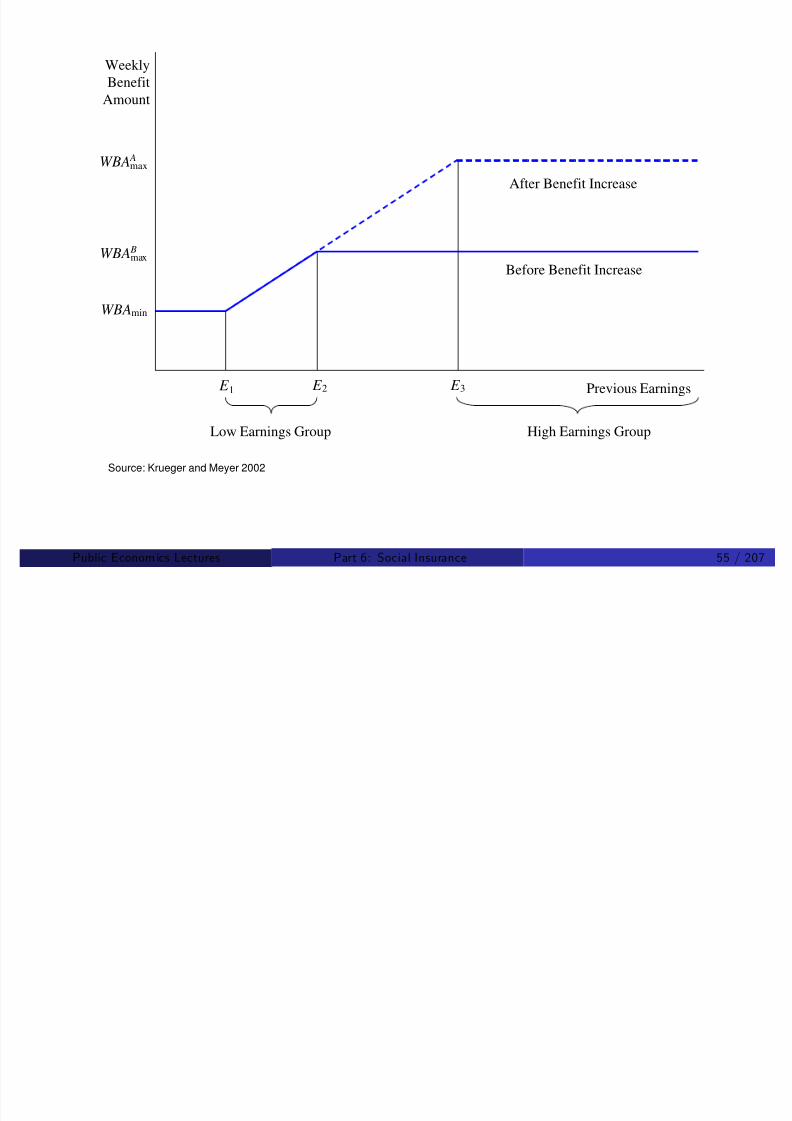
8/8/2019 Chetty - Public Economics Lectures
http://slidepdf.com/reader/full/chetty-public-economics-lectures 661/949
Here αt is the non-parametric “baseline” hazard rate in each period t
and X is a set of covariates
Semi-parametric speci…cation – allow hazards to vary freely acrossweeks and only identify coe¢cients o¤ of variation across spells
Public Econom ics Lectures () Part 6: Social Insurance 56 / 207
Hazard Models
Useful to rewrite expression as:
log ht = log αt + βX
Key assumption: e¤ect of covariates proportional across all weeks
d log ht
dX = β =
d log hs
dX 8t , s
If a change in a covariate doubles hazard in week 1, it is forced todouble hazard in week 2 as well
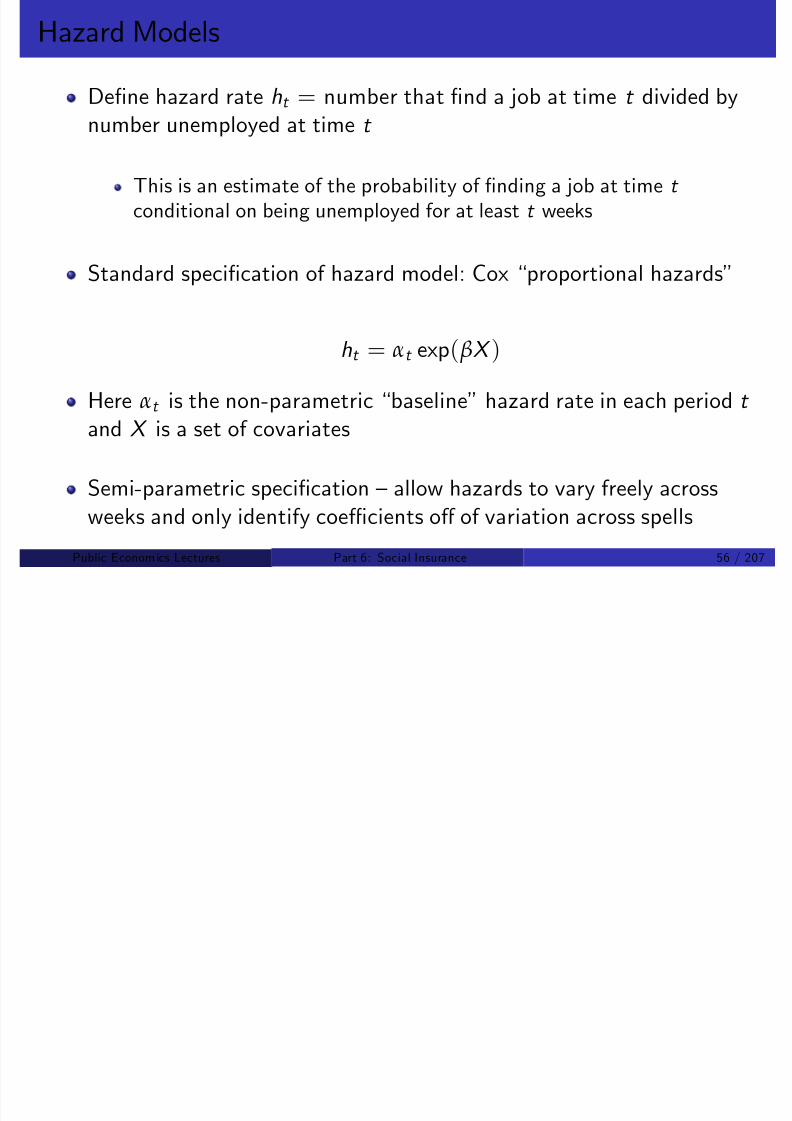
8/8/2019 Chetty - Public Economics Lectures
http://slidepdf.com/reader/full/chetty-public-economics-lectures 662/949
double hazard in week 2 as well
Restrictive but a good starting point; can be relaxed by allowing fortime varying covariates X t
Public Econom ics Lectures () Part 6: Social Insurance 57 / 207
Meyer 1990
Meyer includes log UI bene…t level as a covariate:
log ht = log αt + β1 log b + β2X
In this speci…cation,
d log ht
d log b = β1 = εht ,b
Note: in exponential survival (constant-hazard) models,
εht ,b = ε1e ,b
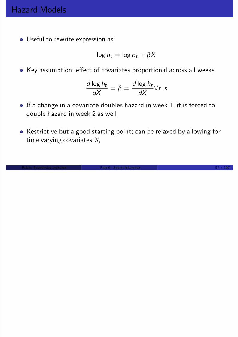
8/8/2019 Chetty - Public Economics Lectures
http://slidepdf.com/reader/full/chetty-public-economics-lectures 663/949
Meyer estimates εht ,b = 0.9 using administrative data for UIclaimants
Subsequent studies get smaller estimates; consensus: εht ,b = 0.5(Krueger and Meyer 2002)
Public Econom ics Lectures () Part 6: Social Insurance 58 / 207
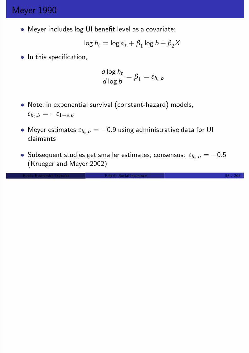
8/8/2019 Chetty - Public Economics Lectures
http://slidepdf.com/reader/full/chetty-public-economics-lectures 664/949
Public Econom ics Lectures () Part 6: Social Insurance 59 / 207
Consumption Smoothing Bene…ts of UI
Gruber (1997) takes the Baily formula to the data by estimatingconsumption smoothing response.
Same methodology as Meyer
Uses cross-state and time variation and uses drop in food consumption
as the LHS variable.
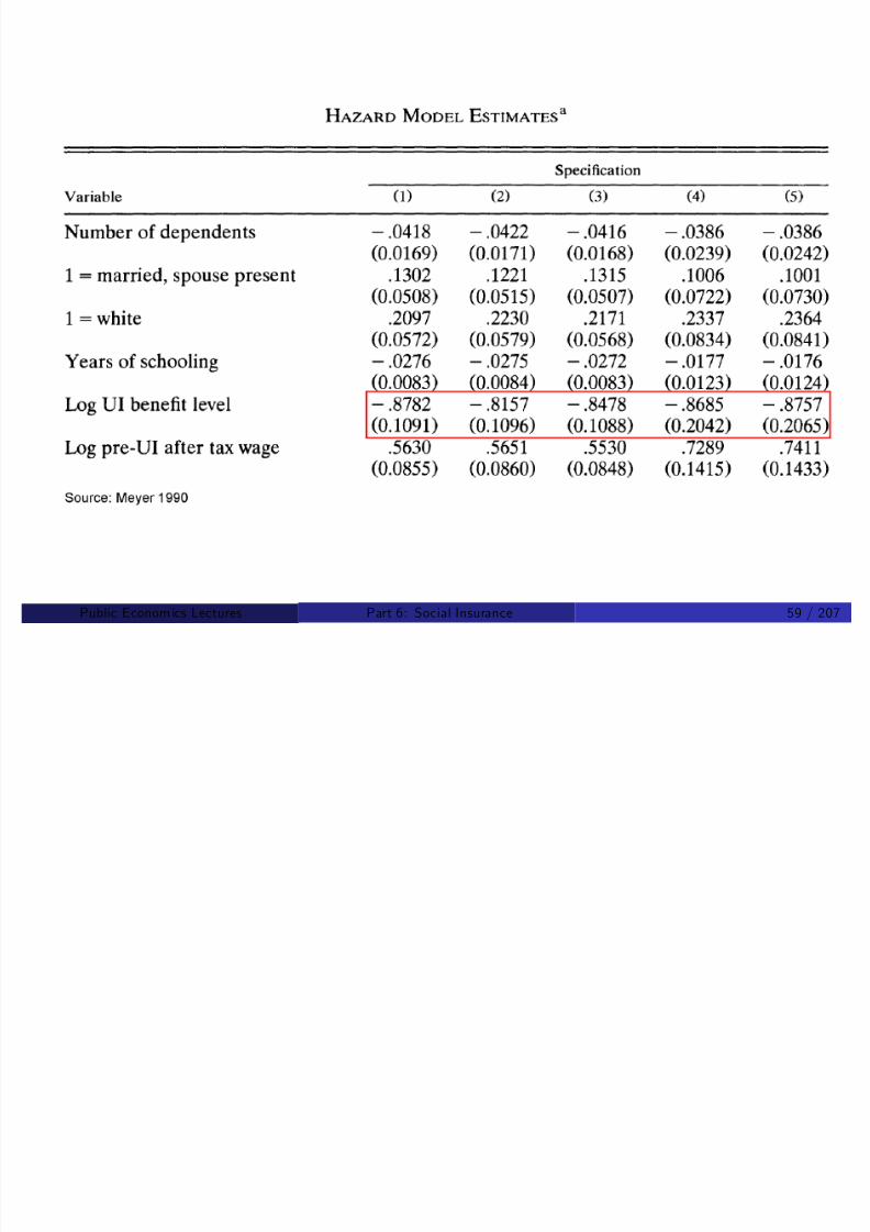
8/8/2019 Chetty - Public Economics Lectures
http://slidepdf.com/reader/full/chetty-public-economics-lectures 665/949
Data: PSID food consumption
Public Econom ics Lectures () Part 6: Social Insurance 60 / 207
Gruber 1997
Gruber estimates∆c
c = β1 + β2
b
w
Finds β1 = 0.24, β2 =
0.28
Without UI, cons drop would be about 24%
Mean drop with current bene…t level (b = 0.5) is about 10%
Implies a 10 pp increase in UI replacement rate causes 2.8 pp

8/8/2019 Chetty - Public Economics Lectures
http://slidepdf.com/reader/full/chetty-public-economics-lectures 666/949
reduction in cons. drop
Convincing evidence that ins. markets are not perfect and UI does
play a consumption smoothing role
Public Econom ics Lectures () Part 6: Social Insurance 61 / 207
Consumption Smoothing Bene…ts of UI
What is substituting for/getting crowded out by UI?
Cullen and Gruber (2000) emphasize spousal labor supply
Study wives of unemployed husbands
Examine wives’ labor supply as a fn of level of husbands’ UI bene…ts
For a $100/wk increase in UI bene…t, wives work 22 hrs less per month
In the absence of UI, wives would work 30% more during the spell than

8/8/2019 Chetty - Public Economics Lectures
http://slidepdf.com/reader/full/chetty-public-economics-lectures 667/949
, % g pthey do now
Engen and Gruber (1995) document that higher UI bene…ts lower
ex-ante savings, another crowdout channel
Public Econom ics Lectures () Part 6: Social Insurance 62 / 207
Calibrating the Model
Gruber calibrates Baily’s model using his and Meyer’s estimates:
γ∆c
c ε1e ,b
e
γ( β1 + β2
b
w ) =
ε1
e ,b
e
Solving for the optimal replacement rate yields:
b
w
=ε1e ,b /e
β2
(1
γ
)
β1
β2
Pl i i 43 i G b (1997) d 95 (5%

8/8/2019 Chetty - Public Economics Lectures
http://slidepdf.com/reader/full/chetty-public-economics-lectures 668/949
Plugging in ε1e ,b = .43 as in Gruber (1997) and e = .95 (5%unemployment rate) yields:
b
w = (.43/.95
.28 1
γ ) (.24)
.28
Public Econom ics Lectures () Part 6: Social Insurance 63 / 207
Calibrating the Model
Results: b w
varies considerably with γ
γ 1 2 3 4 5 10b w
0 0.05 0.31 0.45 0.53 0.7
Gruber: introspection and existing evidence suggests γ < 2
) optimal program small (i.e. replacement rates should be muchlower than is observed)
Surprising result in view of $200bn income security expenditure

8/8/2019 Chetty - Public Economics Lectures
http://slidepdf.com/reader/full/chetty-public-economics-lectures 669/949
Surprising result in view of $200bn income security expenditure
Parameter that is most poorly identi…ed: γ
Risk preferences appear to vary substantially according to situation.
Public Econom ics Lectures () Part 6: Social Insurance 64 / 207
Chetty and Szeidl (2007): Consumption Commitments
Standard expected utility model: one composite consumption good c
Composite commodity assumes that people can cut back on allconsumption goods at all times freely.
E.g. when unemployed, cut consumption of food, housing, cars,furniture, etc.
In practice di¢cult to adjust many elements of consumption in short

8/8/2019 Chetty - Public Economics Lectures
http://slidepdf.com/reader/full/chetty-public-economics-lectures 670/949
In practice, di¢cult to adjust many elements of consumption in shortrun because of …xed adjustment costs
Public Econom ics Lectures () Part 6: Social Insurance 65 / 207
- . 0 7 5
- . 0 5
- . 0 2 5
0
. 0 2 5
.
0 5
F o o d a n d H o u s i n
g G r o w t h R a t e s
4 2 0 2 4
Homeowners’ Consumption around Unemployment Shocks

8/8/2019 Chetty - Public Economics Lectures
http://slidepdf.com/reader/full/chetty-public-economics-lectures 671/949
-4 -2 0 2 4
dyear
Housing (Home Value) Food
Source: Chetty and Szeidl 2007
Public Econom ics Lectures () Part 6: Social Insurance 66 / 207
- . 0 7 5
- . 0 5
- . 0 2 5
0
. 0 2 5
. 0 5
F o o d a n d H o u s i n
g G r o w t h R a t e s
4 2 0 2 4
Renters’ Consumption around Unemployment Shocks

8/8/2019 Chetty - Public Economics Lectures
http://slidepdf.com/reader/full/chetty-public-economics-lectures 672/949
-4 -2 0 2 4
dyear
Housing (Rent) Food
Source: Chetty and Szeidl 2007
Public Econom ics Lectures () Part 6: Social Insurance 67 / 207
Commitments and Risk Aversion
How do commitments a¤ect risk aversion?
Utility over two goods, food and housing:
U (f , h) = u (f ) + v (h).
Adjusting h requires payment of a …xed cost k

8/8/2019 Chetty - Public Economics Lectures
http://slidepdf.com/reader/full/chetty-public-economics-lectures 673/949
j g q p y
Agent follows an (S , s ) policy
Public Econom ics Lectures () Part 6: Social Insurance 68 / 207

8/8/2019 Chetty - Public Economics Lectures
http://slidepdf.com/reader/full/chetty-public-economics-lectures 674/949
Public Econom ics Lectures () Part 6: Social Insurance 69 / 207
Commitments Model: Implications for UI
Commitments amplify risk aversion
Ex: 50% food, 50% housingSuppose unemployed agent forced to cut expenditure by 10%
Then have to cut food cons by 20%, leading to larger welfare loss
Model of commitments suggests that γ might actually exceed 4 forunemployment shocks
γ 1 2 3 4 5 10b 0 0 05 0 31 0 45 0 53 0 7

8/8/2019 Chetty - Public Economics Lectures
http://slidepdf.com/reader/full/chetty-public-economics-lectures 675/949
w 0 0.05 0.31 0.45 0.53 0.7
Problem: γ hard to estimate precisely by context
Public Econom ics Lectures () Part 6: Social Insurance 70 / 207
Alternative Formulas for Optimal UI
Since γ and ∆c c
are hard to identify, recent work has soughtalternative ways of calculating optimal bene…t.
Two approaches
1 Moral hazard vs. liquidity (Chetty 2008)
2 Reservation wage response (Shimer Werning 2007)

8/8/2019 Chetty - Public Economics Lectures
http://slidepdf.com/reader/full/chetty-public-economics-lectures 676/949
Note that any formula is only one representation of optimal bene…t
Public Econom ics Lectures () Part 6: Social Insurance 71 / 207
Chetty 2008: Moral Hazard vs. Liquidity
Discrete time dynamic search model
Individual lives for T periods
Interest rate and discount rate equal to 0
Individual loses job in period t = 0
Let u (c t ) denote ‡ow utility over cons.
Dynamic budget constraint:

8/8/2019 Chetty - Public Economics Lectures
http://slidepdf.com/reader/full/chetty-public-economics-lectures 677/949
Dynamic budget constraint:
At +1 = At + y t c t
Asset limit: At L
Public Econom ics Lectures () Part 6: Social Insurance 72 / 207
Chetty 2008: Baseline Assumptions
1 Assets prior to job loss exogenous
2 No heterogeneity
3 Fixed wages: choose only search intensity, not reservation wage
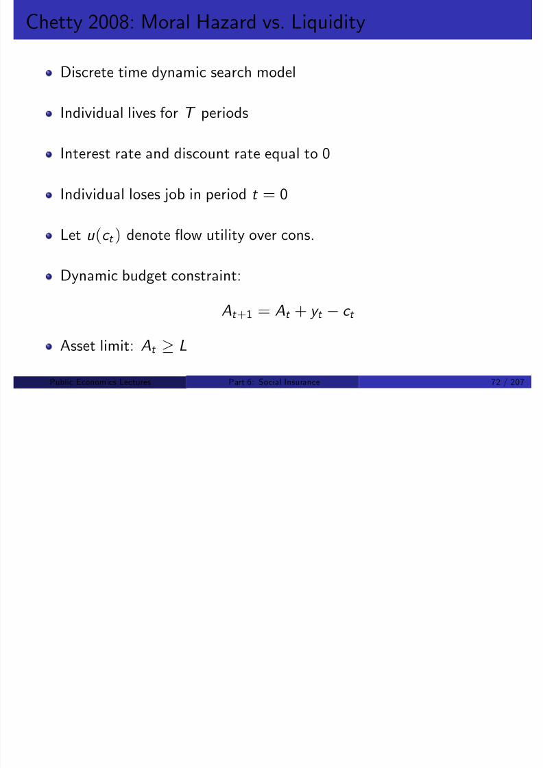
8/8/2019 Chetty - Public Economics Lectures
http://slidepdf.com/reader/full/chetty-public-economics-lectures 678/949
Each of these is relaxed in paper, so model nests search models usedin structural literature (e.g. Wolpin 1987)
Public Econom ics Lectures () Part 6: Social Insurance 73 / 207
Chetty 2008: Job Search Technology
If unemployed in period t , worker …rst chooses search intensity s t
Finds a job that begins immediately in period t with probability s t
If job found, consumes c e t . Jobs are permanent, pay wage w t
τ .
8/8/2019 Chetty - Public Economics Lectures
http://slidepdf.com/reader/full/chetty-public-economics-lectures 679/949
Public Econom ics Lectures () Part 6: Social Insurance 74 / 207
Chetty 2008: Job Search Technology
If no job found: receives bene…t b t , consumes c u t , enters t + 1
unemployed
Cost of job search: ψ(s t )
Period t
c t e = c
t+1e = …
c tu
s t
1-s t
s t+1 c t+1
e
Period t
c t e = c
t+1e = …
c tu
s t
1-s t
s t+1 c t+1
e

8/8/2019 Chetty - Public Economics Lectures
http://slidepdf.com/reader/full/chetty-public-economics-lectures 680/949
t
1-s t+1 c
t+1u
t
1-s t+1 c
t+1u
Public Econom ics Lectures () Part 6: Social Insurance 75 / 207
Chetty 2008: Value Functions
Value function for agent who …nds a job in period t :
V t (At ) = maxAt +1L
u (At At +1 + w τ ) + V t +1(At +1)
Value function for agent who does not …nd a job in period t :
U t (At ) = maxAt +1L
u (At At +1 + b t ) + J t +1(At +1)
where J t +1
(At +1
) is value of entering next period unemployed.
Agent chooses s to maximize expected utility

8/8/2019 Chetty - Public Economics Lectures
http://slidepdf.com/reader/full/chetty-public-economics-lectures 681/949
Agent chooses s t to maximize expected utility
J t (At ) = maxs t
s t V t (At ) + (1 s t )U t (At ) ψ(s t )
Public Econom ics Lectures () Part 6: Social Insurance 76 / 207
Chetty 2008: Optimal Search Behavior
First order condition for optimal search intensity:
ψ0(s t ) = V t (At ) U t (At )
Intuitively, s t is chosen to equate the marginal cost of search e¤ortwith the marginal value of search e¤ort.
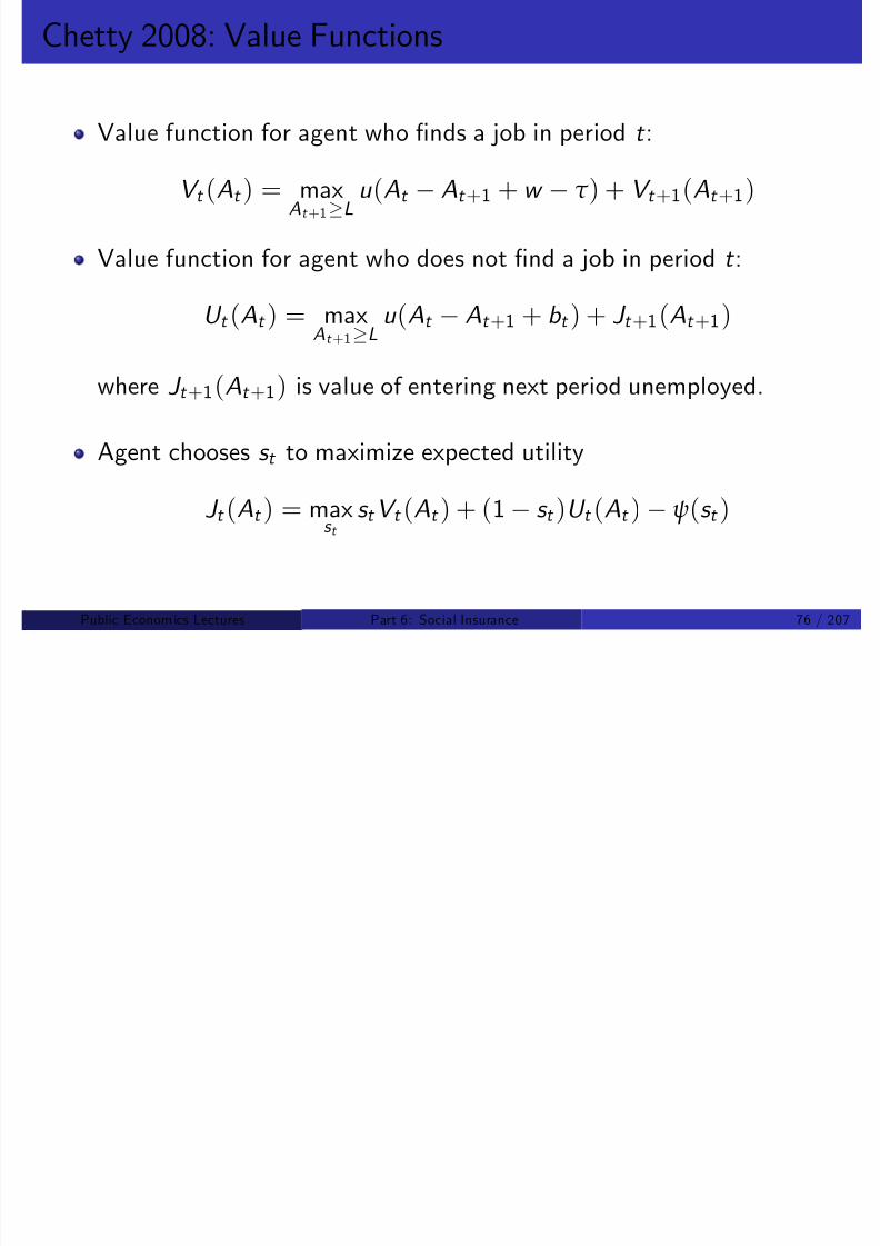
8/8/2019 Chetty - Public Economics Lectures
http://slidepdf.com/reader/full/chetty-public-economics-lectures 682/949
E¤ect of bene…ts on durations:
∂s t /∂b t =
u 0(c u
t )/ψ00(s t )
Public Econom ics Lectures () Part 6: Social Insurance 77 / 207
Chetty 2008: Moral Hazard vs. Liquidity Decomposition
Bene…t e¤ect can be decomposed into two terms:
∂s t /∂At = fu 0(c e t ) u 0(c u
t )g/ψ00(s t ) < 0
∂s t /∂w t = u 0(c e
t
)/ψ00(s t ) > 0
) ∂s t /∂b t = ∂s t /∂At ∂s t /∂w t
∂s t /∂At is “liquidity e¤ect”
∂ /∂ i “ l h d” i ¤

8/8/2019 Chetty - Public Economics Lectures
http://slidepdf.com/reader/full/chetty-public-economics-lectures 683/949
∂s t /∂w t is “moral hazard” or price e¤ect
Liquidity and total bene…t e¤ects smaller for agents with betterconsumption smoothing capacity
Public Econom ics Lectures () Part 6: Social Insurance 78 / 207
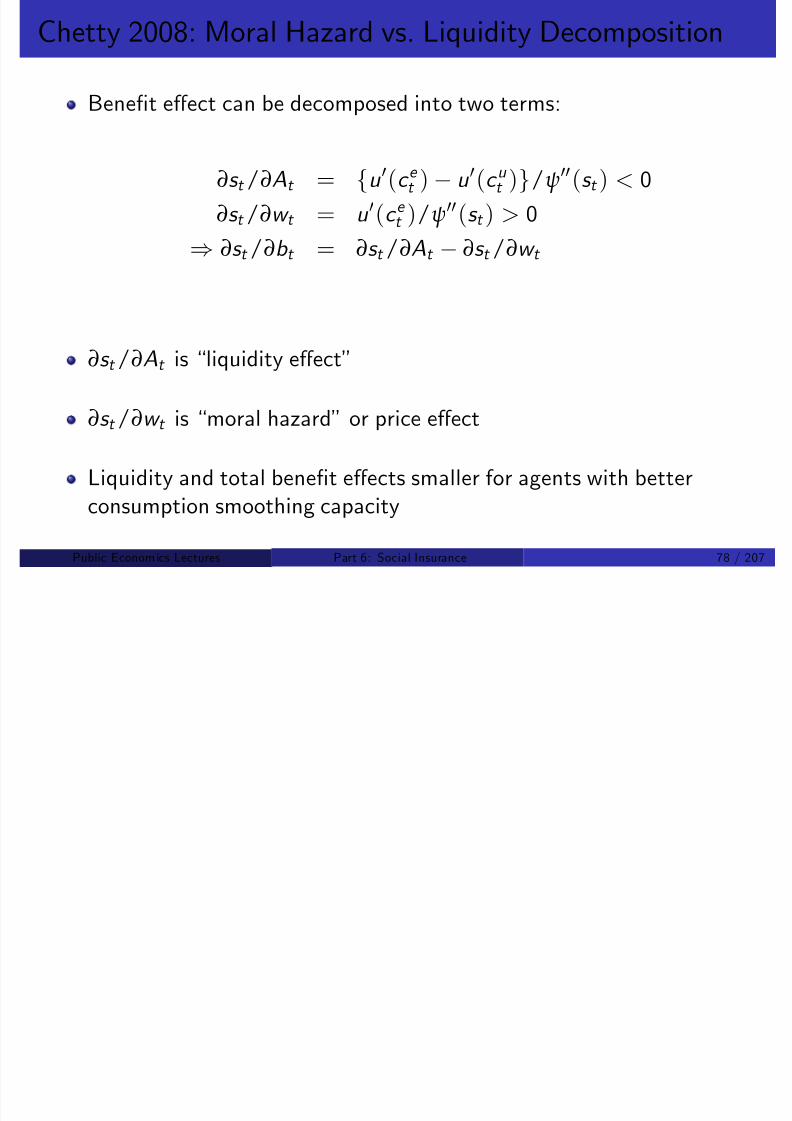
8/8/2019 Chetty - Public Economics Lectures
http://slidepdf.com/reader/full/chetty-public-economics-lectures 684/949
Source: Chetty 2008
Public Econom ics Lectures () Part 6: Social Insurance 79 / 207
Chetty 2008: Formula for Optimal UI
∂s t /∂At = fu 0(c e t ) u 0(c u
t )g/ψ00(s t ) 0
∂s t /∂w t = u 0(c e t )/ψ
00(s t ) > 0
)∂s t /∂At
∂s t /∂w t
=LIQ
MH
=u 0(c u
t ) u 0(c e t )
u 0(c e t )
Can show that the Baily formula holds in this model:
u 0(c u t ) u 0(c e
t )
u 0(c e t )
=ε1e ,b
e
Combining yields formula that depends solely on duration elasticities:
∂ /∂A

8/8/2019 Chetty - Public Economics Lectures
http://slidepdf.com/reader/full/chetty-public-economics-lectures 685/949
∂s t /∂At
∂s t /∂b t ∂s t /∂At =
ε1e ,b
e ε1
e ,A
ε1e ,b Ab
ε1e ,A=
ε1
e ,b
e
Public Econom ics Lectures () Part 6: Social Insurance 80 / 207
Intuition for Moral Hazard vs. Liquidity Formula
Formula is a “revealed preference” approach to valuing insurance
Infer value of UI to agent by observing what he would do if moneygiven as a cash-grant without distorted incentives
If agent would not use money to extend duration, infer that only takeslonger because of price subsidy (moral hazard)
But if he uses cash grant to extend duration, indicates that UIfacilitates a choice he would make if markets were complete
Same strategy can be used in valuing other types of insurance

8/8/2019 Chetty - Public Economics Lectures
http://slidepdf.com/reader/full/chetty-public-economics-lectures 686/949
Make inferences from agent’s choices instead of directly computingcosts and bene…ts of the policy
Key assumption: perfect agent optimization
Public Econom ics Lectures () Part 6: Social Insurance 81 / 207
Moral Hazard vs. Liquidity: Evidence
Two empirical strategies
1 Divide agents into liquidity constrained and unconstrained groups andestimate e¤ect of bene…ts on durations using changes in UI laws.
2 Look at lump-sum severance payments to estimate liquidity e¤ect.
8/8/2019 Chetty - Public Economics Lectures
http://slidepdf.com/reader/full/chetty-public-economics-lectures 687/949
Public Econom ics Lectures () Part 6: Social Insurance 82 / 207
Summary Statistics by Wealth Quartile for SIPP Sample
TABLE 1
1 2 3 4(< -$1,115) (-$1,115-$128) ($128-$13,430) (>$13,430)
Median Liq. Wealth $466 $0 $4,273 $53,009Median Debt $5,659 $0 $353 $835Median Home Equity $2,510 $0 $11,584 $48,900Median Annual Wage $17,188 $14,374 $18,573 $23,866
Mean Years of Education 12.21 11.23 12.17 13.12Mean Age 35.48 35.18 36.64 41.74
Fraction Renters 0.43 0.61 0.35 0.16Fraction Married 0.64 0.59 0.60 0.63
Net Liquid Wealth Quartile

8/8/2019 Chetty - Public Economics Lectures
http://slidepdf.com/reader/full/chetty-public-economics-lectures 688/949
All monetary variables in real 1990 dollars
Source: Chetty 2008
Public Econom ics Lectures () Part 6: Social Insurance 83 / 207
. 2
. 4
. 6
. 8
1
F r a c t i o n U n e
m p l o y e d
0 10 20 30 40 50
Effect of UI Benefits on Durations: Lowest Quartile of Net Wealth
Figure 3a
Mean rep. rate = .53
Mean rep. rate = .48
Wilcoxon Test for Equality: p = 0.01

8/8/2019 Chetty - Public Economics Lectures
http://slidepdf.com/reader/full/chetty-public-economics-lectures 689/949
0 10 20 30 40 50Weeks Unemployed
Avg. UI benefit below mean Avg. UI benefit above mean
Source: Chetty 2008
Public Econom ics Lectures () Part 6: Social Insurance 84 / 207
. 2
. 4
. 6
. 8
1
F r a c t i o n U n e
m p l o y e d
0 10 20 30 40 50
Effect of UI Benefits on Durations: Second Quartile of Net Wealth
Figure 3b
Mean rep. rate = .48
Mean rep. rate = .53
Wilcoxon Test for Equality: p = 0.04

8/8/2019 Chetty - Public Economics Lectures
http://slidepdf.com/reader/full/chetty-public-economics-lectures 690/949
0 10 20 30 40 50Weeks Unemployed
Avg. UI benefit below mean Avg. UI benefit above mean
Source: Chetty 2008
Public Econom ics Lectures () Part 6: Social Insurance 85 / 207
. 2
. 4
. 6
. 8
1
F r a c t i o n U n e m p l o y e d
0 10 20 30 40 50
Effect of UI Benefits on Durations: Third Quartile of Net Wealth
Figure 3c
Mean rep. rate = .46
Mean rep. rate = .52
Wilcoxon Test for Equality: p = 0.69

8/8/2019 Chetty - Public Economics Lectures
http://slidepdf.com/reader/full/chetty-public-economics-lectures 691/949
0 10 20 30 40 50Weeks Unemployed
Avg. UI benefit below mean Avg. UI benefit above mean
Source: Chetty 2008
Public Econom ics Lectures () Part 6: Social Insurance 86 / 207
. 2
. 4
. 6
. 8
1
F r a c t i o n U n e m p l o y e d
0 10 20 30 40 50
Effect of UI Benefits on Durations: Highest Quartile of Net Wealth
Figure 3d
Mean rep. rate = .43
Mean rep. rate = .52
Wilcoxon Test for Equality: p = 0.43

8/8/2019 Chetty - Public Economics Lectures
http://slidepdf.com/reader/full/chetty-public-economics-lectures 692/949
0 10 20 30 40 50Weeks Unemployed
Avg. UI benefit below mean Avg. UI benefit above mean
Source: Chetty 2008
Public Econom ics Lectures () Part 6: Social Insurance 87 / 207
(1) (2) (3) (4) (5)
Pooled StratifiedFull cntrls No cntrls Avg WBA Max WBA Ind. WBA
log UI ben -0.527
(0.267)
Q1 x log UI ben -0.721 -0.978 -0.727 -0.642
(0.304) (0.398) (0.302) (0.241)
Q2 x log UI ben -0.699 -0.725 -0.388 -0.765
(0.484) (0.420) (0.303) (0.219)
Q3 x log UI ben -0.368 -0.476 -0.091 -0.561
(0.309) (0.358) (0.370) (0.156)
Q4 x log UI ben 0.234 0.103 0.304 0.016
(0.369) (0.470) (0.339) (0.259)
Q1=Q4 p-val 0.039 0.013 0.001 0.090
Q1+Q2=Q3+Q4 p-val 0.012 0.008 0.002 0.062
TABLE 2
Effect of UI Benefits: Cox Hazard Model Estimates
Stratified with Full Controls
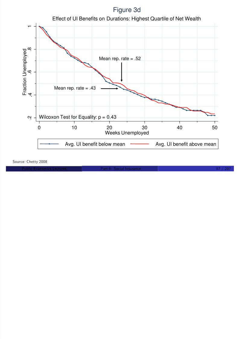
8/8/2019 Chetty - Public Economics Lectures
http://slidepdf.com/reader/full/chetty-public-economics-lectures 693/949
Q Q Q3 Q p a 0 0 0 008 0 00 0 06
Number of Spells 4529 4337 4054 4054 4054
Source: Chetty 2008
Public Econom ics Lectures () Part 6: Social Insurance 88 / 207
$30,693$19,347$20,848Median pre-unemp annual wage
4.81.51.9Median job tenure (years)
$30,693$19,347$20,848Median pre-unemp annual wage
4.81.51.9Median job tenure (years)
(0.17)(0.83)
SeveranceNo SeverancePooled
Summary Statistics for Mathematica Data
TABLE 3
Summary Statistics for Mathematica Data
TABLE 3
40.635.236.2Mean age
68%56%58%Percent married
34%13%17%Percent college grads
6%15%14%Percent dropouts
40.635.236.2Mean age
68%56%58%Percent married
34%13%17%Percent college grads
6%15%14%Percent dropouts

8/8/2019 Chetty - Public Economics Lectures
http://slidepdf.com/reader/full/chetty-public-economics-lectures 694/949
j (y )j (y )
Source: Chetty 2008
Public Econom ics Lectures () Part 6: Social Insurance 89 / 207
. 5
. 6
. 7
. 8
. 9
1
F r a c t i o n U n e m p l o y e d
0 5 10 15 20
Effect of Severance Pay on Durations
Figure 5

8/8/2019 Chetty - Public Economics Lectures
http://slidepdf.com/reader/full/chetty-public-economics-lectures 695/949
Weeks Unemployed
No Severance Received Severance
Source: Chetty 2008
Public Econom ics Lectures () Part 6: Social Insurance 90 / 207
. 4
. 6
. 8
1
F r a c t i o n U n e m p l o y e d
0 5 10 15 20
Effect of Severance Pay on Durations: Below Median Net Wealth
Figure 6a

8/8/2019 Chetty - Public Economics Lectures
http://slidepdf.com/reader/full/chetty-public-economics-lectures 696/949
Weeks Unemployed
No Severance Received Severance
Source: Chetty 2008
Public Econom ics Lectures () Part 6: Social Insurance 91 / 207
. 4
. 6
. 8
1
F r a c t i o n U n e m p l o y e d
0 5 10 15 20
Effect of Severance Pay on Durations: Above Median Net Wealth
Figure 6b
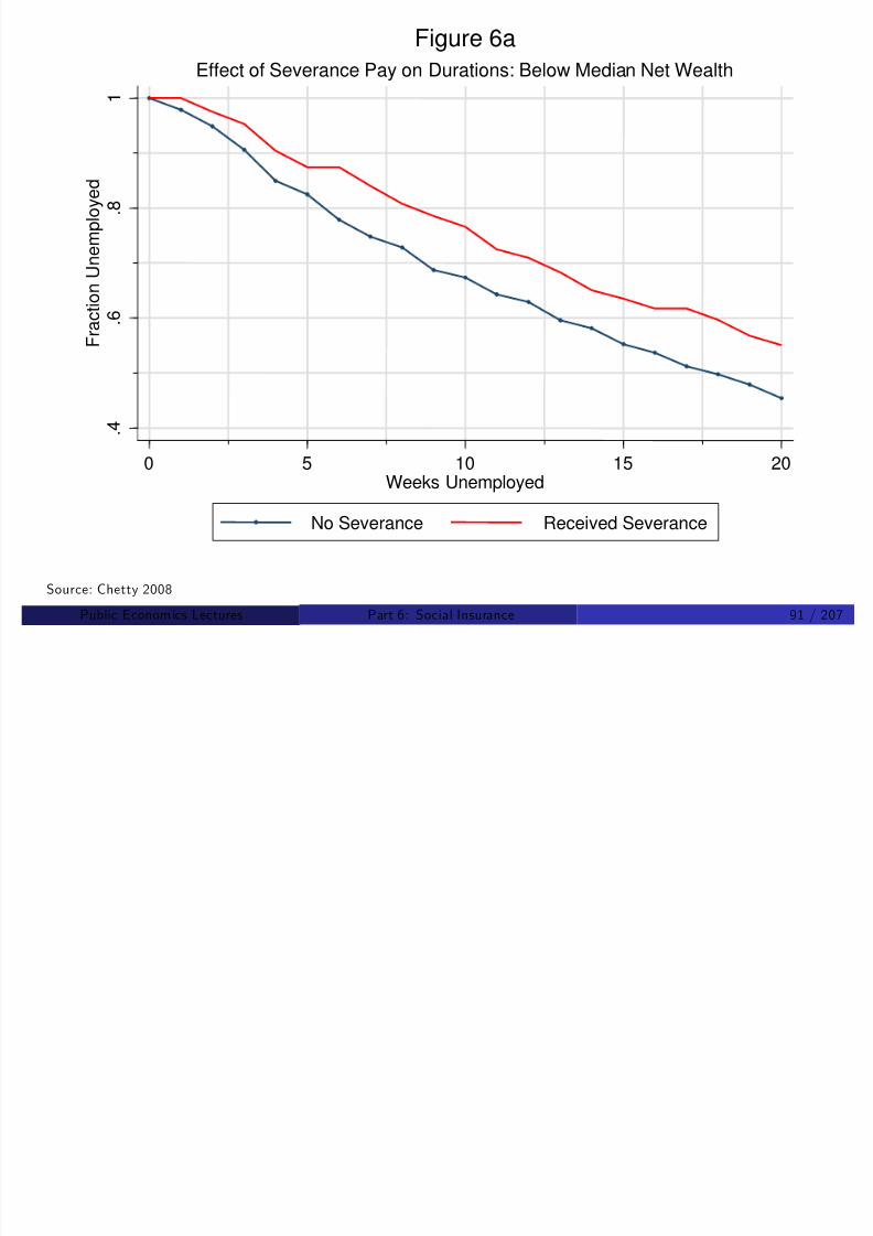
8/8/2019 Chetty - Public Economics Lectures
http://slidepdf.com/reader/full/chetty-public-economics-lectures 697/949
Weeks Unemployed
No Severance Received Severance
Source: Chetty 2008
Public Econom ics Lectures () Part 6: Social Insurance 92 / 207
Pooled By Liquid Wealth By Sev. Amt.
Severance Pay -0.233
(0.071)
(Netliq < Median) x Sev Pay -0.457
(0.099)
(Netliq > Median) x Sev Pay -0.088
(0.081)
(Tenure < Median) x Sev Pay -0.143
(0.055)
(Tenure > Median) x Sev Pay -0.340
(0.119)
TABLE 4
Effect of Severance Pay: Cox Hazard Model Estimates
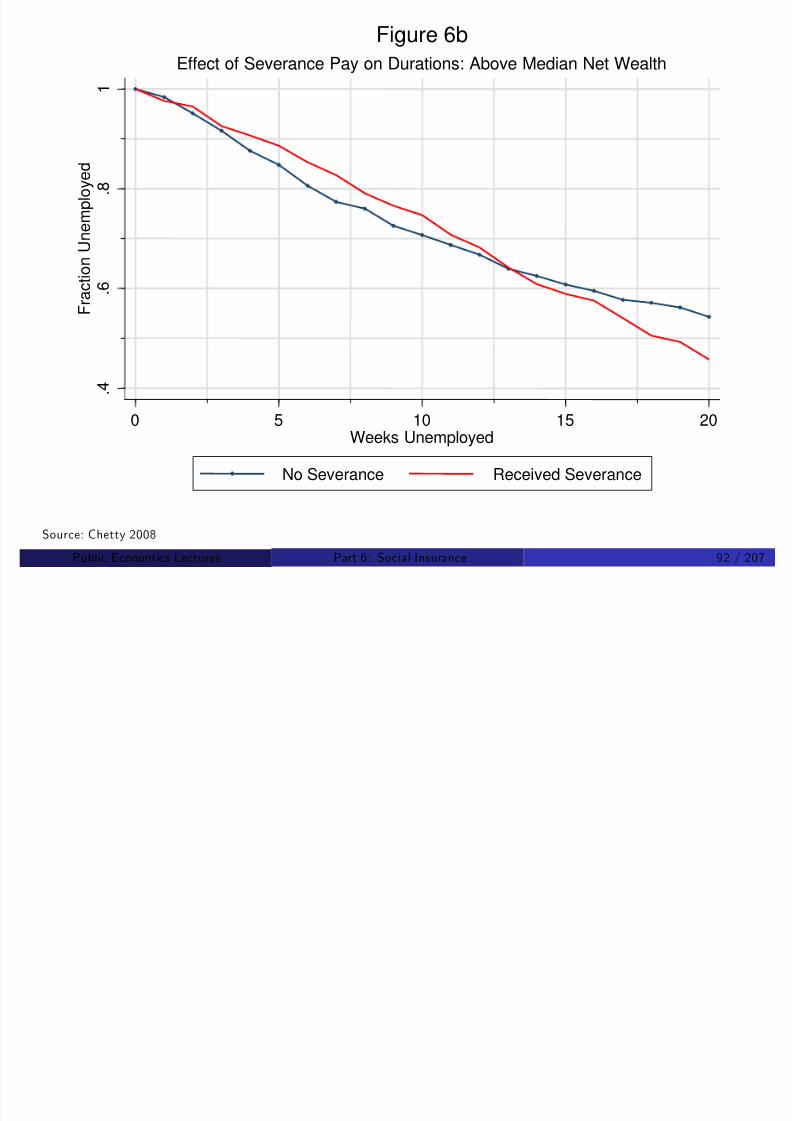
8/8/2019 Chetty - Public Economics Lectures
http://slidepdf.com/reader/full/chetty-public-economics-lectures 698/949
Equality of coeffs p-val <0.01 0.03
N=2428; all specs. include full controls.
Source: Chetty 2008
Public Econom ics Lectures () Part 6: Social Insurance 93 / 207
Chetty 2008: Implications for Optimal UI
Plug reduced-form estimates of de /dA and de /db into formula tocalculate dW /db
Welfare gain from raising bene…t level by 10% from current level inU.S. (50% wage replacement) is $5.9 bil = 0.05% of GDP
Small but positive
In structural models calibrated to match su¢cient statistics, dW /db falls rapidly with b
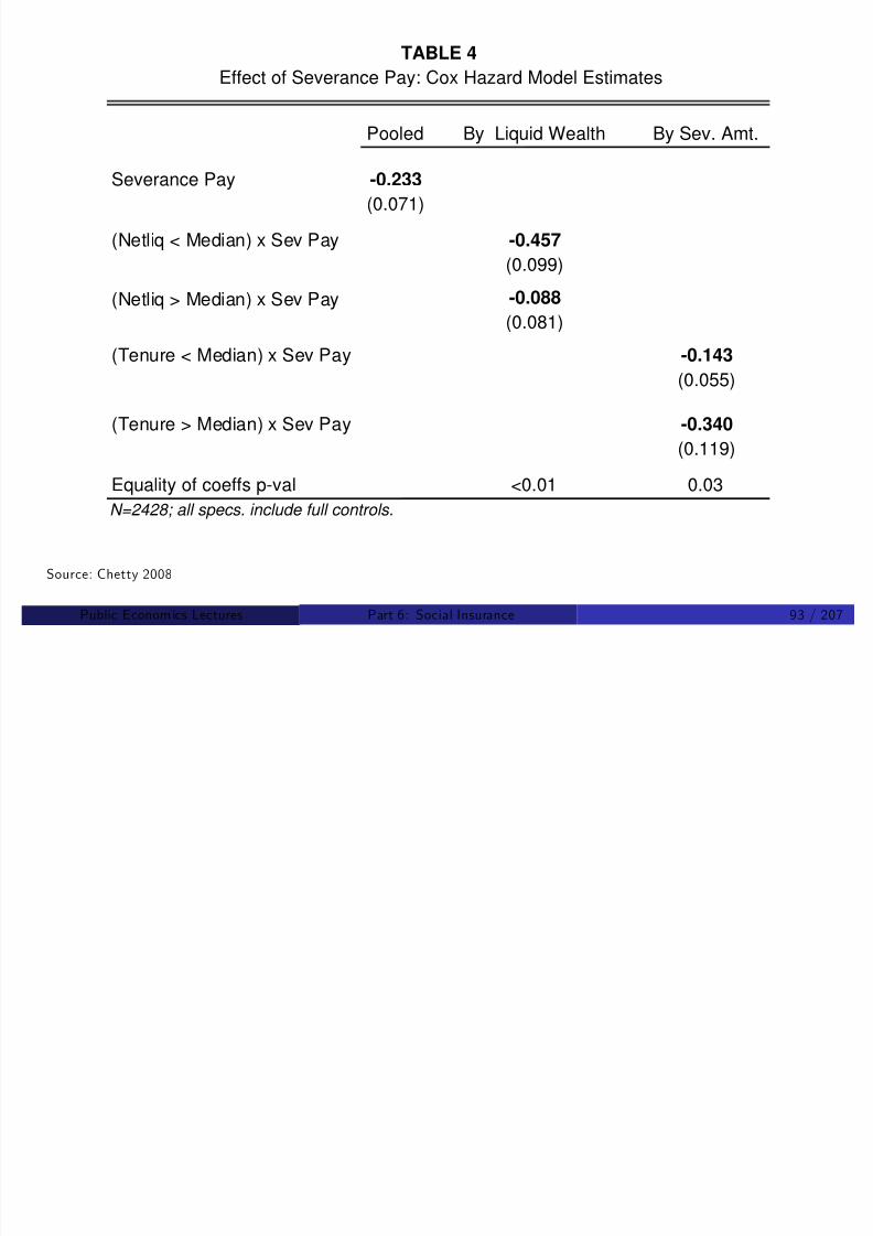
8/8/2019 Chetty - Public Economics Lectures
http://slidepdf.com/reader/full/chetty-public-economics-lectures 699/949
Small dW /db suggests we are currently near optimal bene…t level
Public Econom ics Lectures () Part 6: Social Insurance 94 / 207
Card, Chetty, and Weber 2007
Use discontinuities in Austria’s unemployment bene…t system toestimate liquidity e¤ects
Severance payment is made by …rms out of their own funds
Formula for sev. pay amount for all non-construction workers:
S e v e r a n c
e A m t .
( m o n t h s o f p a y )
3
2
0

8/8/2019 Chetty - Public Economics Lectures
http://slidepdf.com/reader/full/chetty-public-economics-lectures 700/949
0 36 60
Job Tenure
0
Public Econom ics Lectures () Part 6: Social Insurance 95 / 207
0
1
0 0 0 0
2 0 0 0 0
3 0 0 0 0
4 0 0 0
0
N u m b e r o f L a y o f f s
Frequency of Layoffs by Job Tenure
Figure 3

8/8/2019 Chetty - Public Economics Lectures
http://slidepdf.com/reader/full/chetty-public-economics-lectures 701/949
12 18 24 30 36 42 48 54 60
Previous Job Tenure (Months)
Source: Card, Chetty, and Weber 2007
Public Econom ics Lectures () Part 6: Social Insurance 96 / 207
3 0
3 1
3 2
3 3
3 4
M e a n A
g e
12 18 24 30 36 42 48 54 60
Age by Job Tenure
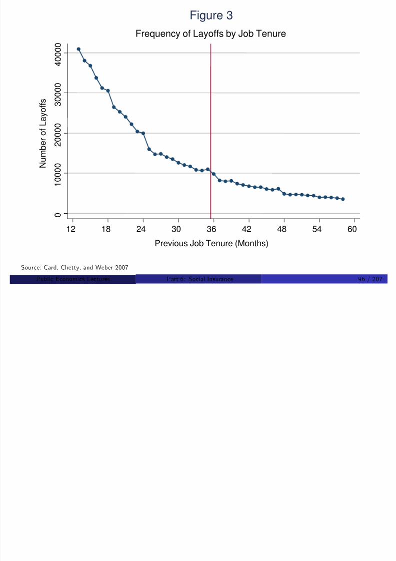
8/8/2019 Chetty - Public Economics Lectures
http://slidepdf.com/reader/full/chetty-public-economics-lectures 702/949
12 18 24 30 36 42 48 54 60
Previous Job Tenure (Months)
Source: Card, Chetty, and Weber 2007
Public Econom ics Lectures () Part 6: Social Insurance 97 / 207
. 8
. 8 5
. 9
. 9
5
M e a n P r e d i c t e d H a z
a r d R a t i o s
Selection on Observables
Figure 4

8/8/2019 Chetty - Public Economics Lectures
http://slidepdf.com/reader/full/chetty-public-economics-lectures 703/949
12 18 24 30 36 42 48 54 60
Previous Job Tenure (Months)
Source: Card, Chetty, and Weber 2007
Public Econom ics Lectures () Part 6: Social Insurance 98 / 207
1 4 5
1 5 0
1 5 5
1 6 0
1 6 5
M e a n N o n e m p l o y m e n t D
u r a t i o n
( d a y s )
Effect of Severance Pay on Nonemployment Durations
Figure 5a
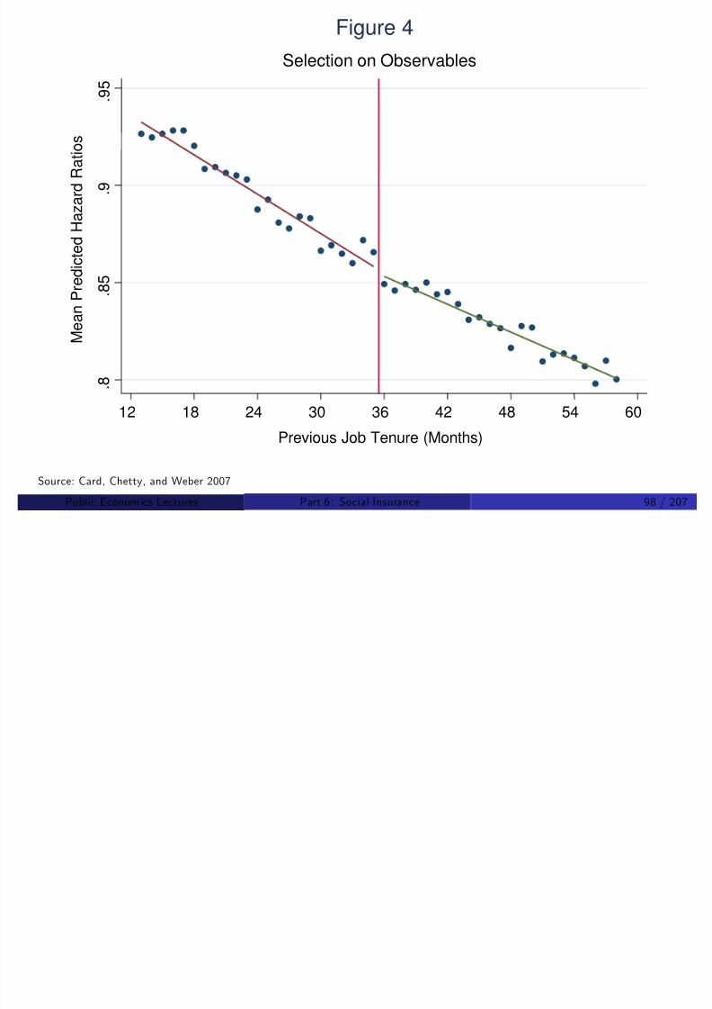
8/8/2019 Chetty - Public Economics Lectures
http://slidepdf.com/reader/full/chetty-public-economics-lectures 704/949
12 18 24 30 36 42 48 54 60
Previous Job Tenure (Months)
Source: Card, Chetty, and Weber 2007
Public Econom ics Lectures () Part 6: Social Insurance 99 / 207
RestrictedSample
FullSample
650,922512,767512,767Sample size
(0.016)(0.018)
-0.093-0.084Extended benefits
(0.017)(0.019)
-0.125-0.122Severance pay
RestrictedSample
(3)(2)(1)
Effects of Severance Pay and EB on Durations: Hazard Model Estimates
TABLE 3a
RestrictedSample
FullSample
650,922512,767512,767Sample size
(0.016)(0.018)
-0.093-0.084Extended benefits
(0.017)(0.019)
-0.125-0.122Severance pay
RestrictedSample
(3)(2)(1)
Effects of Severance Pay and EB on Durations: Hazard Model Estimates
TABLE 3a
NOTE--All specs are Cox hazard models that include cubic polynomials with

8/8/2019 Chetty - Public Economics Lectures
http://slidepdf.com/reader/full/chetty-public-economics-lectures 705/949
NOTE--All specs are Cox hazard models that include cubic polynomials withinteractions with sevpay and/or extended benefit dummy.
Source: Card, Chetty, and Weber 2007
Public Econom ics Lectures () Part 6: Social Insurance 100 / 207
Shimer and Werning 2007: Reservation-Wage Model
Reservation wage model: probability of …nding job (e ) determined bydecision to accept or reject a wage o¤er, not search e¤ort
Wage o¤ers drawn from distribution w F (x )
Agent rejects o¤er if net wage w t is less than outside option b ,implying that probability of …nding a job is e = 1 F (b + t )
Agent’s expected value prior to job search:
W (b ) = (1 F (b + t ))E [u (w t )jw t > b ] + F (b + t )u (b )
Reservation wage prior to job search satis…es

8/8/2019 Chetty - Public Economics Lectures
http://slidepdf.com/reader/full/chetty-public-economics-lectures 706/949
Reservation wage prior to job search satis…es
u (w 0 t ) = W (b )
Public Econom ics Lectures () Part 6: Social Insurance 101 / 207
Shimer and Werning 2007: Reservation-Wage Formula
Government’s problem is
max W (b ) = max u (w 0
t ) = max w 0
t
It follows that
dW
db =
d w 0
db dt
db
= d w 0db
1 e e
(1 + 1e
ε1e ,b )

8/8/2019 Chetty - Public Economics Lectures
http://slidepdf.com/reader/full/chetty-public-economics-lectures 707/949
Public Econom ics Lectures () Part 6: Social Insurance 102 / 207
Shimer and Werning 2007: Reservation-Wage Formula
Implement formula using estimates of d w 0db
reported by Feldstein andPoterba (1984)
Find gains from raising UI bene…ts 5 times larger than Chetty (2008)
But reservation wage elasticity estimates questionable
Do greater bene…ts ! longer durations ! better outcomes later on?No.
Ex: evidence from Austrian discontinuity (Card, Chetty, Weber 2007)

8/8/2019 Chetty - Public Economics Lectures
http://slidepdf.com/reader/full/chetty-public-economics-lectures 708/949
Note: all the formulas above take such match quality gains intoaccount via envelope conditions
Public Econom ics Lectures () Part 6: Social Insurance 103 / 207
1 4 5
1 5 0
1 5 5
1 6 0
1 6 5
M e a n N o n e m p l o y m e n t D
u r a t i o n
( d a y s )
Effect of Severance Pay on Nonemployment Durations
Figure 5a

8/8/2019 Chetty - Public Economics Lectures
http://slidepdf.com/reader/full/chetty-public-economics-lectures 709/949
12 18 24 30 36 42 48 54 60
Previous Job Tenure (Months)
Source: Card, Chetty, and Weber 2007
Public Econom ics Lectures () Part 6: Social Insurance 104 / 207
- . 1
- . 0
8
- . 0 6
- . 0 4
- . 0 2
0
W a g e G r o w
t h
Effect of Severance Pay on Subsequent Wages
Figure 10a
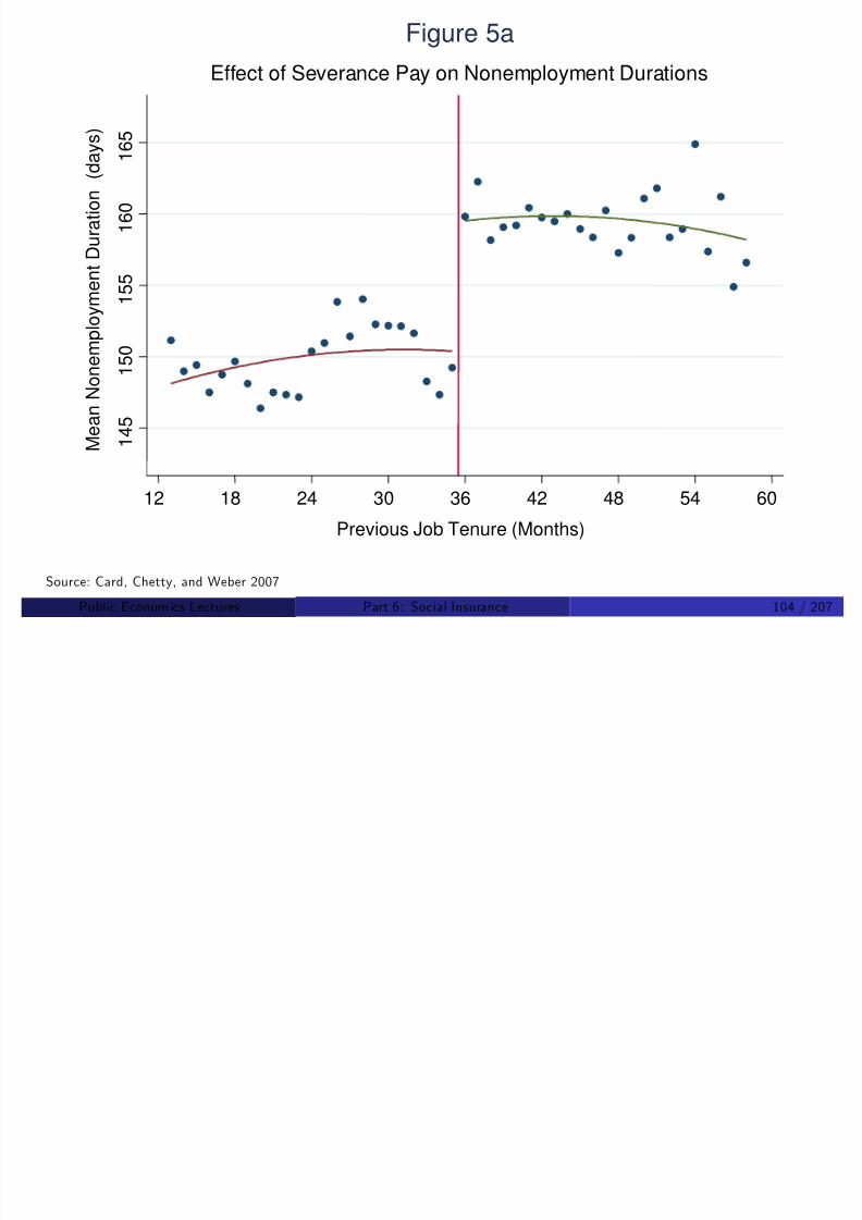
8/8/2019 Chetty - Public Economics Lectures
http://slidepdf.com/reader/full/chetty-public-economics-lectures 710/949
12 18 24 30 36 42 48 54 60
Previous Job Tenure (Months)
Source: Card, Chetty, and Weber 2007
Public Econom ics Lectures () Part 6: Social Insurance 105 / 207
- . 0 5
0
. 0 5
. 1
. 1 5
. 2
A v e r a g e M o n t h l y J o b E n d i n g
H a z a r d i n N e x t J o b
Effect of Severance Pay on Subsequent Job Duration
Figure 10b

8/8/2019 Chetty - Public Economics Lectures
http://slidepdf.com/reader/full/chetty-public-economics-lectures 711/949
12 18 24 30 36 42 48 54 60
Previous Job Tenure (Months)
Source: Card, Chetty, and Weber 2007
Public Econom ics Lectures () Part 6: Social Insurance 106 / 207
1 3 5
1
4 0
1 4 5
1 5 0
1 5 5
1 6 0
1 6 5
M e a n
N o n e m p l o y m e n t D
u r a t i o n
( d a y s )
12 18 24 30 36 42 48 54 60
Effect of Benefit Extension on Nonemployment Durations
Figure 9a

8/8/2019 Chetty - Public Economics Lectures
http://slidepdf.com/reader/full/chetty-public-economics-lectures 712/949
12 18 24 30 36 42 48 54 60
Months Employed in Past Five Years
Source: Card, Chetty, and Weber 2007
Public Econom ics Lectures () Part 6: Social Insurance 107 / 207
- . 1
- . 0 5
0
. 0 5
. 1
W a g e G
r o w t h
12 18 24 30 36 42 48 54 60
Effect of Extended Benefits on Subsequent Wages

8/8/2019 Chetty - Public Economics Lectures
http://slidepdf.com/reader/full/chetty-public-economics-lectures 713/949
Months Worked in Past Five Years
Source: Card, Chetty, and Weber 2007
Public Econom ics Lectures () Part 6: Social Insurance 108 / 207
- . 1 5
- . 1
- . 0 5
0
. 0 5
A v e r a g e
M o n t h l y J o b E n d
i n g H a z a r d i n N e x
t J o b
12 18 24 30 36 42 48 54 60
Effect of Extended Benefits on Subsequent Job Duration

8/8/2019 Chetty - Public Economics Lectures
http://slidepdf.com/reader/full/chetty-public-economics-lectures 714/949
Months Worked in Past Five Years
Source: Card, Chetty, and Weber 2007
Public Econom ics Lectures () Part 6: Social Insurance 109 / 207
Spike at Bene…t Exhaustion
Most striking evidence for distortionary e¤ects of social insurance:“spike” in hazard rate at bene…t exhaustion
Katz and Meyer (1990), Meyer (1990), ...
Traditional measure of hazard: exiting UI system
Preferred measure based on theory: …nding a job
The two could di¤er if workers transit o¤ of UI but are still jobless
Ex. may not go to pick up last unemployment check

8/8/2019 Chetty - Public Economics Lectures
http://slidepdf.com/reader/full/chetty-public-economics-lectures 715/949
Particularly important in European context, where you can remain
registered on UI inde…nitely
Public Econom ics Lectures () Part 6: Social Insurance 110 / 207
0
. 0 5
. 1
. 1 5
. 2
U n e m p l o y m e n t E x i t H a z a r d
20 15 10 5 0
Time Until Benefits Lapse Empirical Hazard

8/8/2019 Chetty - Public Economics Lectures
http://slidepdf.com/reader/full/chetty-public-economics-lectures 716/949
20 15 10 5 0
Weeks of Eligibility LeftSource: Meyer 1990
Public Econom ics Lectures () Part 6: Social Insurance 111 / 207
0
. 0 5
. 1
. 1 5
. 2
W e e k l y H a z a r d R a t e
0 10 20 30 40 50
Weeks Elapsed Since Job Loss
Job Finding Hazards Unemp Exit Hazards
Job Finding vs. Unemployment Exit Hazards: 20 Week UI

8/8/2019 Chetty - Public Economics Lectures
http://slidepdf.com/reader/full/chetty-public-economics-lectures 717/949
Job Finding Hazards Unemp Exit Hazards
Source: Card, Chetty, Weber 2007b (AER P&P)
Public Econom ics Lectures () Part 6: Social Insurance 112 / 207
0
. 0 5
. 1
. 1 5
. 2
W e e k l y H
a z a r d R a t e
0 10 20 30 40 50
Weeks Elapsed Since Job Loss
Job Finding Hazards Unemp Exit Hazards
Job Finding vs. Unemployment Exit Hazards: 30 Week UI
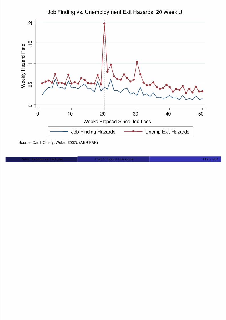
8/8/2019 Chetty - Public Economics Lectures
http://slidepdf.com/reader/full/chetty-public-economics-lectures 718/949
Job Finding Hazards Unemp Exit Hazards
Source: Card, Chetty, Weber 2007b (AER P&P)
Public Econom ics Lectures () Part 6: Social Insurance 113 / 207
- . 1
- . 0 5
0
. 0 5
. 1
D
i f f e r e n c e i n W e e k
l y H a z a r d U I 2 0 - U I 3 0
0 10 20 30 40 50
Weeks Elapsed Since Job Loss
Unemployment Exit Hazards Job Finding Hazards
Effect of Benefit Expiration on Hazard Rates

8/8/2019 Chetty - Public Economics Lectures
http://slidepdf.com/reader/full/chetty-public-economics-lectures 719/949
U e p oy e t t a a ds Job d g a a ds
Source: Card, Chetty, Weber 2007b (AER P&P)
Public Econom ics Lectures () Part 6: Social Insurance 114 / 207
UI and Firm Behavior
Preceding discussion assumed perfect experience rating of UI
Firms’ layo¤ incentives are not distorted
But in practice, UI is not perfectly experience rated
Feldstein (1976, 1978) shows:
Theoretically that imperfect experience rating e¤ect can raise rate of temporary layo¤s
Empirically that this e¤ect is large in practice
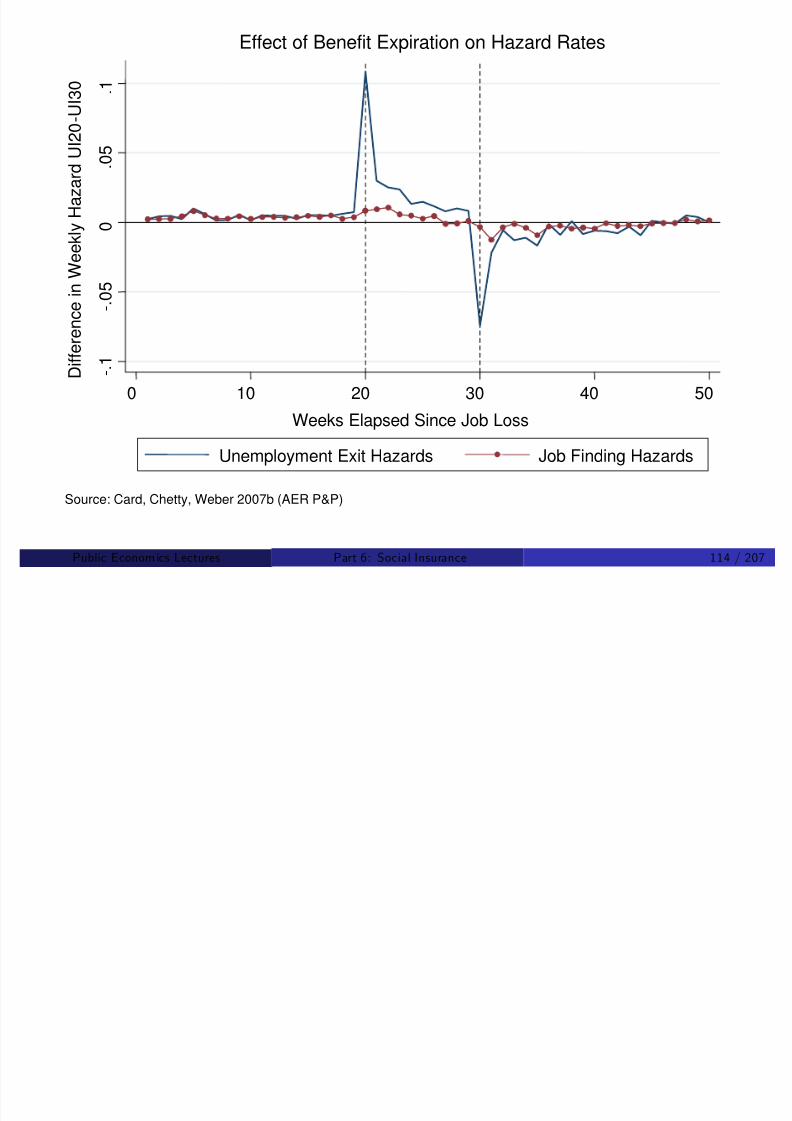
8/8/2019 Chetty - Public Economics Lectures
http://slidepdf.com/reader/full/chetty-public-economics-lectures 720/949
p y g p
Public Econom ics Lectures () Part 6: Social Insurance 115 / 207
0
2
4
6
8
1 0
U I T a x
R a t e ( % )
0 2 4 6 8 10
Benefit Ratio (100*UI Benefits Paid/Payroll)
Experience Rating in Washington, 2005

8/8/2019 Chetty - Public Economics Lectures
http://slidepdf.com/reader/full/chetty-public-economics-lectures 721/949
Washington’s UI Tax Schedule Perfect Experience Rating
Source: Washington State Joint Legislative Task Force on Unemployment Insurance Benefit Equity 2005
Public Econom ics Lectures () Part 6: Social Insurance 116 / 207
UI and Firm Behavior: Feldstein 1976 model
Firms o¤er workers stochastic contracts, with wage and probability of temporary layo¤
Two states: high demand and low demand
In equilibrium, competitive …rms will o¤er contract that pays workerhis marginal product in expectation over two states at cheapest costto …rm
Firm pro…ts by laying o¤ workers with imperfect exp rating
Layo¤s generate …rst-order gain in pro…ts at a second-order cost fromadded risk to worker
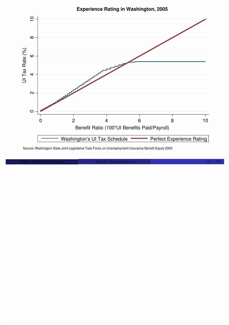
8/8/2019 Chetty - Public Economics Lectures
http://slidepdf.com/reader/full/chetty-public-economics-lectures 722/949
In an imperfectly experience-rated economy, …rms choose a positiverate of layo¤s in low output state
Public Econom ics Lectures () Part 6: Social Insurance 117 / 207
Feldstein 1978: Empirical Results
First observation: more than half of …rms are above the max rate orbelow the min rate
No marginal incentive for these …rms to reduce layo¤s.
Uses cross-state/time variation in UI bene…ts
10% increase in UI bene…ts causes a 7% increase in temp layo¤
unemployment
E¤ect is twice as large for union members as non-union, suggestingworker-…rm coordination

8/8/2019 Chetty - Public Economics Lectures
http://slidepdf.com/reader/full/chetty-public-economics-lectures 723/949
worker …rm coordination.
Public Econom ics Lectures () Part 6: Social Insurance 118 / 207
Topel 1983
Feldstein does not directly show that imperfect exp rating is to blamefor more temp layo¤s b/c not using variation in experience rating itself
Topel (1983) uses state/industry variation in …nancing of UI
Variation in tax rate on …rms from min/max thresholds for exp rating
Finds that imperfect subsidization accounts for 31% of all temp layo¤ unemployment, a very large e¤ect
See Krueger and Meyer (2002) for review of more recent studies,which …nd similar results but smaller magnitudes

8/8/2019 Chetty - Public Economics Lectures
http://slidepdf.com/reader/full/chetty-public-economics-lectures 724/949
Public Econom ics Lectures () Part 6: Social Insurance 119 / 207
UI Savings Accounts
Alternative to UI transfer-based system (Feldstein and Altman 2007)
Instead of paying UI tax to government, pay into a UI savings account.If unemployed, deplete this savings account according to currentbene…t schedule
If savings exhausted, government pays bene…t as in current system(…nanced using a tax).
Idea: people internalize loss of money from staying unemp longer.
Reduces distortion from UI while providing bene…ts as in currentsystem.But modelling this formally is di¢cult: to internalize incentives atretirement people must be forward looking but then no need to force

8/8/2019 Chetty - Public Economics Lectures
http://slidepdf.com/reader/full/chetty-public-economics-lectures 725/949
retirement, people must be forward looking, but then no need to force
them to save.
Public Econom ics Lectures () Part 6: Social Insurance 120 / 207
Feldstein and Altman 2007
Address feasibility: How many people hit negative balance on UIaccount and just go back to old system?
Simulate how UI savings accounts would evolve using actual earnings
histories from PSID.
Calculations imply that only 1/3 of spells will occur with negativebalances, so most people still have good incentives while unemployed.
Total tax payments are less than half what they are in current system.
In their simulation, bene…ts are identical; only question is how costschange
8/8/2019 Chetty - Public Economics Lectures
http://slidepdf.com/reader/full/chetty-public-economics-lectures 726/949
change.
Public Econom ics Lectures () Part 6: Social Insurance 121 / 207
Feldstein and Altman 2007
Calculation of changes in present value of lifetime wealth from switchto UISA by income quintile:
Q1 Q2 Q3 Q4 Q5Present Value Gain: -$95 +$22 -$67 +$94 +$468
Net PVG is positive
Without change in behavior, how is the pie larger?
Reason: discounting at 2% but earning 5 5% interest
8/8/2019 Chetty - Public Economics Lectures
http://slidepdf.com/reader/full/chetty-public-economics-lectures 727/949
Reason: discounting at 2% but earning 5.5% interest
Public Econom ics Lectures () Part 6: Social Insurance 122 / 207
Takeup
Mean takeup rate is very low – a major puzzle in this literature(Currie 2004)
Why leave money on the table?
Andersen and Meyer (1997) show that after-tax UI replacement ratea¤ects level of takeup.
So at least some seem to be optimizing at the margin.
Takeup low in many govt. programs. (UI, food stamps, EITC, etc.)
Possible explanations: myopia, stigma, hassle, lack of info.

8/8/2019 Chetty - Public Economics Lectures
http://slidepdf.com/reader/full/chetty-public-economics-lectures 728/949
Public Econom ics Lectures () Part 6: Social Insurance 123 / 207
Black, Smith, Berger, and Noel 2003
Experiment in KY where some UI claimants were randomly assignedto receive re-employment services
E.g., assisted job search, employment counseling, job search workshops,retraining programs
Treatment [N = 1236] required to receive services in order to get UIbene…ts
Control [N = 745]: exempt from services

8/8/2019 Chetty - Public Economics Lectures
http://slidepdf.com/reader/full/chetty-public-economics-lectures 729/949
Public Econom ics Lectures () Part 6: Social Insurance 124 / 207

8/8/2019 Chetty - Public Economics Lectures
http://slidepdf.com/reader/full/chetty-public-economics-lectures 730/949

8/8/2019 Chetty - Public Economics Lectures
http://slidepdf.com/reader/full/chetty-public-economics-lectures 731/949
Public Econom ics Lectures () Part 6: Social Insurance 126 / 207
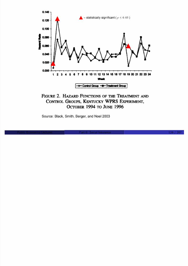
8/8/2019 Chetty - Public Economics Lectures
http://slidepdf.com/reader/full/chetty-public-economics-lectures 732/949
Public Econom ics Lectures () Part 6: Social Insurance 127 / 207
Black, Smith, Berger, and Noel 2003: Results
Treatment group exit UI system earlier, receiving 2.2 fewer weeks of
bene…ts on average
Most signi…cant increase in exits in wks 2-3, when noti…ed of mandatory services

8/8/2019 Chetty - Public Economics Lectures
http://slidepdf.com/reader/full/chetty-public-economics-lectures 733/949
Public Econom ics Lectures () Part 6: Social Insurance 128 / 207
General Equilibrium: Acemoglu and Shimer 1999
UI can be e¢ciency-enhancing in equilibrium.
Standard models focus only on distortionary costs, and assume thattotal output always lower when UI is provided.
But this ignores potentially important GE e¤ect: more risky jobsprovided in eq. if workers are insured.
Provision of UI raises availability of risky jobs (e.g. tech jobs) and can
raise e¢ciency in equilibrium
So if workers are risk averse, tradeo¤ may not be very hard – bothraise output and insure them better.
8/8/2019 Chetty - Public Economics Lectures
http://slidepdf.com/reader/full/chetty-public-economics-lectures 734/949
p
Public Econom ics Lectures () Part 6: Social Insurance 129 / 207
Dynamics: Path of UI Bene…ts
Classic reference is Shavell and Weiss (1979), who solved for optimalpath of bene…ts in a 3 period model.
Tradeo¤: upward sloping path ! more moral hazard but more
consumption-smoothing bene…ts.
Recent literature that is very active in this area: “new dynamic public…nance” – optimal path of unemployment and disability programs.
Hopenhayn and Nicolini (1997) – numerical simulations for case wheregovt can control consumption
Shimer and Werning (2008) – with perfect liquidity and CARA utility,optimal bene…t path is ‡at

8/8/2019 Chetty - Public Economics Lectures
http://slidepdf.com/reader/full/chetty-public-economics-lectures 735/949
optimal bene…t path is ‡at
Public Econom ics Lectures () Part 6: Social Insurance 130 / 207
Optimal Insurance in Behavioral Models
We do not have a model consistent with the data that can explainboth savings behavior pre-unemployment and search behaviorpost-unemployment
Evidence that unemployment is indeed costly and bene…ts can improvewelfare a lot for certain liquidity-constrained groups
Simple rational model cannot rationalize level of savings that peoplehave when they get unemployed
Interesting direction for future research: optimal SI with behavioralconsiderations (see e.g., Spinnewijn 2009)

8/8/2019 Chetty - Public Economics Lectures
http://slidepdf.com/reader/full/chetty-public-economics-lectures 736/949
Public Econom ics Lectures () Part 6: Social Insurance 131 / 207
Workers Compensation
Insurance against injury at work
Covers both lost wages and medical bene…ts
Rationales for govt. intervention:
Market may fail due to adverse selection
Workers may be unaware of risks on the job
Litigation costs (origin of system in 1920s)
Substantial variation in bene…ts across states for di¤erent injuries
8/8/2019 Chetty - Public Economics Lectures
http://slidepdf.com/reader/full/chetty-public-economics-lectures 737/949
Public Econom ics Lectures () Part 6: Social Insurance 132 / 207
Maximum Indemnity Bene…ts (2003)
State Type of permanent impairment Temporary Injury
Arm Hand Index …nger Leg Foot (10 weeks)
California $108,445 $64,056 $4,440 $118,795 $49,256 $6,020
Hawaii 180,960 141,520 26,800 167,040 118,900 5,800
Illinois 301,323 190,838 40,176 276,213 155,684 10,044
Indiana 86,500 62,500 10,400 74,500 50,500 5,880
Michigan 175,657 140,395 24,814 140,395 105,786 6,530
Missouri 78,908 59,521 15,305 70,405 52,719 6,493
New Jersey 154,440 92,365 8,500 147,420 78,200 6,380
New York 124,800 97,600 18,400 115,200 82,000 4,000
S G b (2007)

8/8/2019 Chetty - Public Economics Lectures
http://slidepdf.com/reader/full/chetty-public-economics-lectures 738/949
Source: Gruber (2007)
Public Econom ics Lectures () Part 6: Social Insurance 133 / 207

8/8/2019 Chetty - Public Economics Lectures
http://slidepdf.com/reader/full/chetty-public-economics-lectures 739/949
Outline of Empirical Evidence
1 Monday e¤ects and impact on worker behavior
2 Firm side responses
3 E¤ect on equilibrium wage

8/8/2019 Chetty - Public Economics Lectures
http://slidepdf.com/reader/full/chetty-public-economics-lectures 740/949
Public Econom ics Lectures () Part 6: Social Insurance 135 / 207

8/8/2019 Chetty - Public Economics Lectures
http://slidepdf.com/reader/full/chetty-public-economics-lectures 741/949
Public Econom ics Lectures () Part 6: Social Insurance 136 / 207
Day of the Week E¤ect
Intertemporal distortions, moral hazard e¤ect of workers’ comp.
Card & McCall (1994): test if weekend injuries lead to Monday e¤ect.
Look at uninsured workers, who should have bigger Monday e¤ect.
Find no di¤erence in e¤ect between insured and uninsured.
Other explantations:
Gaming system for more days o¤.
Pure reporting e¤ect if pain does not go away.

8/8/2019 Chetty - Public Economics Lectures
http://slidepdf.com/reader/full/chetty-public-economics-lectures 742/949
Suggests that incentives matter a lot.
Public Econom ics Lectures () Part 6: Social Insurance 137 / 207
E¤ects of Bene…ts on Injuries
Potential incentive e¤ects to look for on worker’s side:
Number of claims of injury
Duration of injuries
Meyer, Viscusi, and Durbin (1995):
Implement DD analysis for workers’ comp durations
Find large e¤ects on duration using reforms in MI and KY

8/8/2019 Chetty - Public Economics Lectures
http://slidepdf.com/reader/full/chetty-public-economics-lectures 743/949
Public Econom ics Lectures () Part 6: Social Insurance 138 / 207

8/8/2019 Chetty - Public Economics Lectures
http://slidepdf.com/reader/full/chetty-public-economics-lectures 744/949
Public Econom ics Lectures () Part 6: Social Insurance 139 / 207

8/8/2019 Chetty - Public Economics Lectures
http://slidepdf.com/reader/full/chetty-public-economics-lectures 745/949
Public Econom ics Lectures () Part 6: Social Insurance 140 / 207
Firm Side Responses
Purchasing insurance leads to imperfect experience rating and moralhazard
Self-insured …rms: stronger incentives to improve safety
Also, have incentive to ensure that workers return to work quickly
Krueger (1990): compares behavior of self-insured …rms with others
Finds self-insured have 10% shorter durations, but selection bias aconcern

8/8/2019 Chetty - Public Economics Lectures
http://slidepdf.com/reader/full/chetty-public-economics-lectures 746/949
Public Econom ics Lectures () Part 6: Social Insurance 141 / 207
E¤ect on Equilibrium Wage
Workers’ compensation is a mandated bene…t
When …rms hire, adjust wage o¤ered to workers downwards b/c theyrealize they must pay bene…t
Summers (1989):
If workers value bene…ts at cost, they bear the full incidenceIf they do not value it, has same e¤ect and DWL as a tax
Gruber-Krueger (1991):
85% of WC cost is shifted to workers, no signi…cant employment e¤ect
Fishback-Kantor (1995):
Find 100% shift to workers’ wages in initial implementation of prog

8/8/2019 Chetty - Public Economics Lectures
http://slidepdf.com/reader/full/chetty-public-economics-lectures 747/949
Suggests that bene…ts valued close to cost
Public Econom ics Lectures () Part 6: Social Insurance 142 / 207
Directions for Further Research on WC
Decomposition into liquidity vs. moral hazard e¤ects
Better evidence on …rm side responses
Consumption smoothing bene…ts

8/8/2019 Chetty - Public Economics Lectures
http://slidepdf.com/reader/full/chetty-public-economics-lectures 748/949
Public Econom ics Lectures () Part 6: Social Insurance 143 / 207
Disability Insurance
See Bound et. al (HLE 1999) for an overview
Insures against long-term shocks that a¤ect individuals at home orwork
Federal program that is part of social security
Eligible if unable to “engage in substantial gainful activity” b/c of
physical/mental impairment for at least one (expected) year
Main focus of literature is sharp rise in the size of the program

8/8/2019 Chetty - Public Economics Lectures
http://slidepdf.com/reader/full/chetty-public-economics-lectures 749/949
Public Econom ics Lectures () Part 6: Social Insurance 144 / 207
0
1
2
3
4
5
6
7
8
9
P
e r c e n t
1950 1960 1970 1980Year
Nonparticipation Rate Social Security Disability Recipiency Rate
Nonparticipation and Recipiency Rates, Men 45-54 Years Old
Source: Parsons 1984 Table A1

8/8/2019 Chetty - Public Economics Lectures
http://slidepdf.com/reader/full/chetty-public-economics-lectures 750/949
Public Econom ics Lectures () Part 6: Social Insurance 145 / 207
Two Views on the Rise in DI
Trend has continued since 1980s: DI share of non-elderly adults rosefrom 3.1% in 1984 to 5.4% in 2000
One perspective on the rise: moral hazard from a lenient system thatleads to ine¢ciency
Another perspective: program is now helping more needy people whohave high disutilities of work
Empirical work attempts to distentangle these two views to someextent

8/8/2019 Chetty - Public Economics Lectures
http://slidepdf.com/reader/full/chetty-public-economics-lectures 751/949
Public Econom ics Lectures () Part 6: Social Insurance 146 / 207

8/8/2019 Chetty - Public Economics Lectures
http://slidepdf.com/reader/full/chetty-public-economics-lectures 752/949
Public Econom ics Lectures () Part 6: Social Insurance 147 / 207
Theory of Disability Insurance
Key additional element relative to UI models is screening and waitingperiods.
Less relevant for unemployment because it is easy to identify who hasa job and who does not.
Diamond-Sheshinski (1995) build a model that incorporates screening.
Characterize optimal properties of solution but do not derive anempirically implementable formula for optimal screening rule orbene…t level.
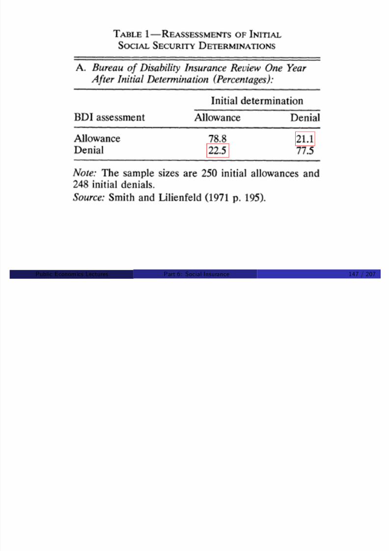
8/8/2019 Chetty - Public Economics Lectures
http://slidepdf.com/reader/full/chetty-public-economics-lectures 753/949
Public Econom ics Lectures () Part 6: Social Insurance 148 / 207
Diamond and Sheshinski 1995
Individuals have di¤erent disutilities of working ψi
To max social welfare, not desirable for those with high ψi to work.
First best: Individual i works i¤
Marginal product > ψi
But govt observes only an imperfect signal of ψi ! sets a higher
threshold for disability
Result: lower bene…t rate if screening mechanism has higher noise tosignal ratio

8/8/2019 Chetty - Public Economics Lectures
http://slidepdf.com/reader/full/chetty-public-economics-lectures 754/949
Public Econom ics Lectures () Part 6: Social Insurance 149 / 207
Empirical Evidence: Bound-Parsons Debate
Question: Did increase in DI bene…ts cause decline in labor supply?
Well-known debate between Bound & Parsons in 1980s
Parsons (1980)
Uses cross-sectional variation in replacement rates
Data on men aged 45-59 in 1966-69 NLSY
OLS regression:LFP i = α + βDIrepratei + εi
where DIreprate is calculated using wage in 1966
Finds elasticity of 0.6
Simulations using this elasticity imply that increase in DI can

8/8/2019 Chetty - Public Economics Lectures
http://slidepdf.com/reader/full/chetty-public-economics-lectures 755/949
completely explain decline in elderly labor force participation
Public Econom ics Lectures () Part 6: Social Insurance 150 / 207
Empirical Evidence: Bound-Parsons Debate
Criticizes Parsons for using an endogenous variable on RHS
Econometric problem: DIreprate = f (wage (); law ) with no variationin law
Identi…cation assumption: LFP rates equal across wage groups
Potential solution: “control” for wage on RHS. Does not make sense.
Bound replicates Parson’s regression on sample that never applied toDI and obtains a similar elasticity

8/8/2019 Chetty - Public Economics Lectures
http://slidepdf.com/reader/full/chetty-public-economics-lectures 756/949
Public Econom ics Lectures () Part 6: Social Insurance 151 / 207
Empirical Evidence: Bound-Parsons Debate
Bound proposes a technique to bound e¤ect of DI on LFP rate
Uses data on LFP of rejected applicants as a counterfactual
Idea: if rejected applicants do not work, then surely DI recipients
would not have worked
Rejected applicants’ LFP rate is an upper bound for LFP rate of DIrecipients absent DI
Results: Only 30% of rejected applicants return to work
Earn less than half of the mean non-DI wage
Implies that at most 1/3 of the trend in male LFP decline can be

8/8/2019 Chetty - Public Economics Lectures
http://slidepdf.com/reader/full/chetty-public-economics-lectures 757/949
explained by shift to DIPublic Econom ics Lectures () Part 6: Social Insurance 152 / 207
8/8/2019 Chetty - Public Economics Lectures
http://slidepdf.com/reader/full/chetty-public-economics-lectures 758/949
Public Econom ics Lectures () Part 6: Social Insurance 153 / 207
Gruber 2000
Exploits di¤erential law change in Quebec and rest of Canada as anatural experiment
In 1987, 36% inc. in bene…ts in rest of Canada; in Quebec, no change
Estimates e¤ect of law change on labor force participation of menaged 45-59
Uses DD method on NLFP rates of men aged 45-59

8/8/2019 Chetty - Public Economics Lectures
http://slidepdf.com/reader/full/chetty-public-economics-lectures 759/949
Public Econom ics Lectures () Part 6: Social Insurance 154 / 207

8/8/2019 Chetty - Public Economics Lectures
http://slidepdf.com/reader/full/chetty-public-economics-lectures 760/949
Public Econom ics Lectures () Part 6: Social Insurance 155 / 207

8/8/2019 Chetty - Public Economics Lectures
http://slidepdf.com/reader/full/chetty-public-economics-lectures 761/949
Public Econom ics Lectures () Part 6: Social Insurance 156 / 207
Gruber 2000
Implied elasticity of NLFP rate w.r.t. DI bene…t level: 0.25-0.3
Agrees more with Bound than Parsons
Limitation of Gruber study (like all DD studies): only estimates shortrun response

8/8/2019 Chetty - Public Economics Lectures
http://slidepdf.com/reader/full/chetty-public-economics-lectures 762/949
Public Econom ics Lectures () Part 6: Social Insurance 157 / 207
Autor and Duggan 2003
Focus on interaction between DI and UI systems
Observe that DI claims rise in recessions, may reduce measuredunemployment rate
Idea: consider a worker laid o¤ in current recession
Given generosity of DI program, instead of claiming UI and searchingfor a job, he applies for DI
One less unemployed person –> unemployment rate lower
But economic situation is the same: one less person working
Test this hypothesis using cross-state variation in employment shocks

8/8/2019 Chetty - Public Economics Lectures
http://slidepdf.com/reader/full/chetty-public-economics-lectures 763/949
Public Econom ics Lectures () Part 6: Social Insurance 158 / 207
Autor and Duggan 2003
Construction of state-level employment shocks over a …ve yearwindow:
Calculate industry shares in a given state in base year
Calculate employment changes over …ve year period by industry usingdata on national employment (excluding state in question)
Project changes in each state’s employment using national changes
Ex: if car industry declines over a …ve year period, assign a negativeemployment shock to Michigan
Then correlate state employment shocks with DI applications

8/8/2019 Chetty - Public Economics Lectures
http://slidepdf.com/reader/full/chetty-public-economics-lectures 764/949
Public Econom ics Lectures () Part 6: Social Insurance 159 / 207

8/8/2019 Chetty - Public Economics Lectures
http://slidepdf.com/reader/full/chetty-public-economics-lectures 765/949
Public Econom ics Lectures () Part 6: Social Insurance 160 / 207
Coefficient = -0.094, se = 0.062, t = -1.51
-8 -6 -4 -2 0 2 4 6 8
-8
-6
-4
-2
0
2
4
6
8
AL
INPAOHRI
NC
VT
AR
TNMT
MEMA
WV
MO
CTIA
MS
MN
IL
GA
NJ
KY
WI
UT
AZ
TX
KSORNE
DE
MI
NY
SD
CO
SCOK
VA
LA
NH
MD
FL
CA
WAND
WYAK ID
NM
HI
NV
Employment Shocks and DI Applications: 1979-1984
E [ D I A p p s
/ P o p | X ]
E[Change in Employment/Pop | X]
Source: Autor and Duggan 2003

8/8/2019 Chetty - Public Economics Lectures
http://slidepdf.com/reader/full/chetty-public-economics-lectures 766/949
Source: Autor and Duggan 2003
Public Econom ics Lectures () Part 6: Social Insurance 161 / 207
Coefficient = -0.262, se = 0.067, t = -3.90
-8
-6
-4
-2
0
2
4
6
8
WV
ND
MS
KY
INOK
SD
NH
MI
KSWYNE
AR
ME
IATN
TXNC
MT
VT
MO
OHPA
MN
DE
SC
IL
GA
MAWI
LA
WA
CT
VA
ALFL
NYCO
UT
RI
NJ
ORCAAZ
NM
MDID
AK
HINV
-6 -4 -2 0 2 4 6 8-8
Employment Shocks and DI Applications: 1984-1989
E [ D I A p p s
/ P o p | X ]
E[Change in Employment/Pop | X]
Source: Autor and Duggan 2003
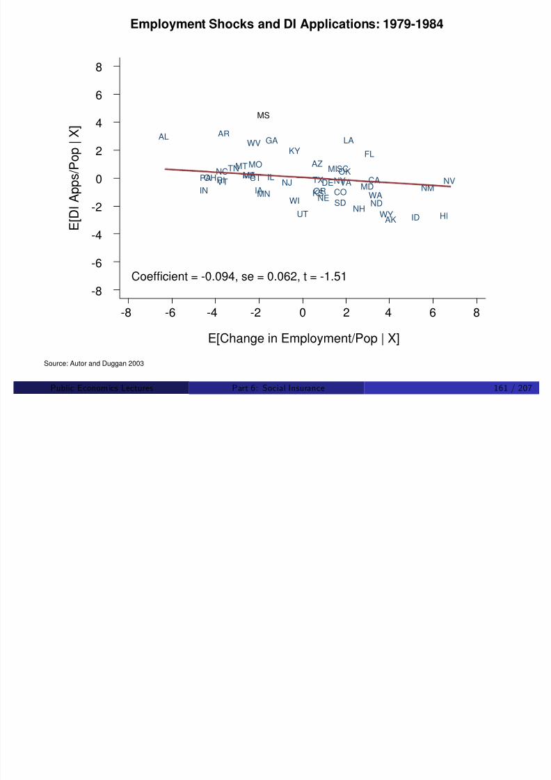
8/8/2019 Chetty - Public Economics Lectures
http://slidepdf.com/reader/full/chetty-public-economics-lectures 767/949
gg
Public Econom ics Lectures () Part 6: Social Insurance 162 / 207
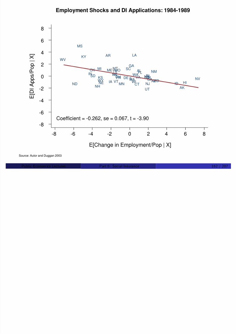
8/8/2019 Chetty - Public Economics Lectures
http://slidepdf.com/reader/full/chetty-public-economics-lectures 768/949
Coefficient = -0.849, se = 0.164 t = -5.18
-8
-6
-4
-2
0
2
4
6
8
WY
AL
AR
AK
WV
MS
ME
SC
KS
ND
GALA
KY
TNNC
OK
MT
SD
UT
NVTXIDNE
WAIA
IN
MO
PAVA
NM
HIOR
DE
AZVT
CAWI
NY
MD
FL
ILCO
OHNJ
MI
MN
CTMANH
RI
-8 -6 -4 -2 0 2 4 6 8
Employment Shocks and DI Applications: 1993-1998
E [ D I A p p s
/ P o p | X ]
E[Change in Employment/Pop | X]
Source: Autor and Duggan 2003

8/8/2019 Chetty - Public Economics Lectures
http://slidepdf.com/reader/full/chetty-public-economics-lectures 769/949
Public Econom ics Lectures () Part 6: Social Insurance 164 / 207
Autor and Duggan 2003
Unemployment would be 0.65% higher if not for post-‘84 trends in DI
participation
Trace decline in LFP to the rise in DI over the past two decades via:
The 1984 inclusion of mental illness in DI eligibility
Rising wage inequality (combined with the progressively of system)
Bottom line: DI applications are clearly sensitive to incentives
But evidence is insu¢cient to make welfare statements
Essential to decompose bene…t e¤ects into income and price elasticitiesto make normative judgment
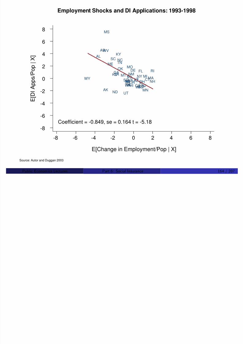
8/8/2019 Chetty - Public Economics Lectures
http://slidepdf.com/reader/full/chetty-public-economics-lectures 770/949
Public Econom ics Lectures () Part 6: Social Insurance 165 / 207
Health Insurance
Arrow (1963): seminal article that described special problems inproviding healthcare using private markets
We will touch upon a few issues in public sector intervention
Health is an important …eld because of enormous size and rapidgrowth.
17% of GDPAnnual growth rate of 3.4% (vs 1.4% growth in GDP)

8/8/2019 Chetty - Public Economics Lectures
http://slidepdf.com/reader/full/chetty-public-economics-lectures 771/949
Public Econom ics Lectures () Part 6: Social Insurance 166 / 207
Year
U.S. Healthcare Spending, 1960-2007
$0
$1000
$2000
$3000
$4000
$5000
$6000
$7000
$8000
$0
$1000
$2000
$3000
$4000
$5000
$6000
$7000
$8000
0%
2.5%
5%
7.5%
10%
12.5%
15%
1960 1965 1970 1975 1980 1985 1990 1995 2000 2005
National Health Expenditure % of GDP
National Health Expenditure Per-Capita $
Source: OECD Health Data (2009)

8/8/2019 Chetty - Public Economics Lectures
http://slidepdf.com/reader/full/chetty-public-economics-lectures 772/949
Public Econom ics Lectures () Part 6: Social Insurance 167 / 207
0
3
6
9
1 2
1 5
K or e a
T ur k e y
M ex i c o
P ol an d
S l ov ak R e p u b l i c
C z e c h R e p u b l i c
I r el an d
L ux em b o ur g
J a p an
U ni t e d K i n g d om
H un g ar y
S p ai n
F i nl an d
A u s t r al i a
N ew
Z e al an d
I t al y
N or w a y
S w e d en
Gr e e c e
I c el an d
D enm ar k
N e t h er l an d s
C an a d a
P or t u g al
B el gi um
A u s t r i a
G er m an y
F r an c e
S wi t z er l an d
U ni t e d S t a t e s
H e a l t h C a r e
S p e n d i n g ( % o f G
D P )
Health Care Spending in OECD Nations in 2005
Source: OECD Health Data (2009)

8/8/2019 Chetty - Public Economics Lectures
http://slidepdf.com/reader/full/chetty-public-economics-lectures 773/949
Public Econom ics Lectures () Part 6: Social Insurance 168 / 207
P
u b l i c S h a r e o
f T o t a
l H e a
l t h S p e n
d i n g
( % )
Public Health Share in OECD Nations, 1960-2007
2 0
3 0
4 0
5 0
6 0
7 0
8 0
9 0
1 0 0
1960 1965 1970 1975 1980 1985 1990 1995 2000 2005
Year
United States
Austria
Norway
Source: OECD Health Data (2009)

8/8/2019 Chetty - Public Economics Lectures
http://slidepdf.com/reader/full/chetty-public-economics-lectures 774/949
Public Econom ics Lectures () Part 6: Social Insurance 169 / 207
People % of
(millions) Population
Total population 288.6 100.00%
Private 177.8 61.60%
• Employment-based 161 55.80%
• Individually purchased 16.8 5.80%Public 83 28.80%
• Medicare 40.5 14.00%
• Medicaid 42.8 14.80%
• Veterans 6.9 2.40%Uninsured 43.3 15.00%
Note: Numbers do not sum to 100% because some people have multiple
coverage. Source: Gruber 2007
Americans’ Source of Health Insurance Coverage, 2002
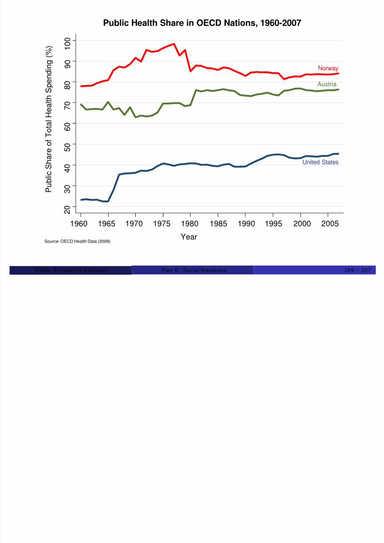
8/8/2019 Chetty - Public Economics Lectures
http://slidepdf.com/reader/full/chetty-public-economics-lectures 775/949
Public Econom ics Lectures () Part 6: Social Insurance 170 / 207
Growing Health Expenditures: Key Factors
1. Fundamentals of supply and demand [market equilibrium]
Demand: Income e¤ect ! more demand (Hall and Jones 2006)
As you get richer, want to live longer, not consume more goodsbecause marginal utility of consumption declines
More sushi dinners, not more sushi per dinner
Supply: technological progress with more expensive methods
Two options for knee surgery: invasive, long recovery [old] vs.arthroscopic [new]. New technology more expensive.
LASIK surgery: expensive but allows you to completely eliminate needfor glasses
Note di¤erence relative to technological progress in other sectors:discovery of more expensive methods rather than reduction in costs of
existing methods

8/8/2019 Chetty - Public Economics Lectures
http://slidepdf.com/reader/full/chetty-public-economics-lectures 776/949
gPublic Econom ics Lectures () Part 6: Social Insurance 171 / 207
Growing Health Expenditures: Key Factors
2. Price Distortions
Demand: government tax subsidy for healthcare and insuranceprograms
Lower e¤ective price for individuals ! overconsumption
Supply: fee-for-service payment schemes
Reimburse physicians for additional procedures ! overproduction

8/8/2019 Chetty - Public Economics Lectures
http://slidepdf.com/reader/full/chetty-public-economics-lectures 777/949
Public Econom ics Lectures () Part 6: Social Insurance 172 / 207
Growing Health Expenditures: Key Factors
3. Regulatory Distortions
Supply of healthcare: malpractice law
Fear of lawsuits ! excess supply of healthcare by physicians
Supply of physicians
Restrictions on number of physicians through medical schoolseats/licensing
American Medical Association acts like a union
Lower supply of physicians ! higher wages and higher input costs

8/8/2019 Chetty - Public Economics Lectures
http://slidepdf.com/reader/full/chetty-public-economics-lectures 778/949
Public Econom ics Lectures () Part 6: Social Insurance 173 / 207
Market Failures and Government Interventions
1. Externalities/Internalities
Sin taxes (alcohol/cigarettes)
Rabin and O’Donoghue (2006): fat tax
2. Consumer myopia
Tax subsidies for health insurance
Samaritan’s Dilemma: government provided insurance
3. Consumers lack information ! suppliers choose level of consumption
Govt. provision of healthcare + …xed physician salaries
Regulation: licensing of doctors, FDA, legal system

8/8/2019 Chetty - Public Economics Lectures
http://slidepdf.com/reader/full/chetty-public-economics-lectures 779/949
Public Econom ics Lectures () Part 6: Social Insurance 174 / 207
Market Failures and Government Interventions
4. Heterogeneity of risk types
!adverse selection in insurance market
5. Ex-ante risk uninsured: cannot contract before birth
6. Equity concerns: health inequality may directly enter social welfare
function
Example: White infant mortality rate is 6 per 1000; black is 14 per1000.
Black child born in DC has lower chance of reaching …rst birthday thanone born in Jamaica.
Solution: government provided health insurance/healthcare

8/8/2019 Chetty - Public Economics Lectures
http://slidepdf.com/reader/full/chetty-public-economics-lectures 780/949
Public Econom ics Lectures () Part 6: Social Insurance 175 / 207
Measuring Health
Before discussing optimal insurance, useful to de…ne a measure of
health consumption
Higher medical expenditure not equivalent to more “health.”
Starting point: mortality.
Need a monetary measure ! measure value of life.
Literature estimates this using many methods (Aldy and Viscusi 2003)
Contingent valuation.Wage premia for risky jobs.Price of smoke detectors.
Commonly used …gure: $100,000 per year of healthy life.

8/8/2019 Chetty - Public Economics Lectures
http://slidepdf.com/reader/full/chetty-public-economics-lectures 781/949
Public Econom ics Lectures () Part 6: Social Insurance 176 / 207
Cutler and Richardson 1997
Propose a better de…nition of value of life that takes quality of life
into account
Measure QALY for several conditions using survey
What is your quality of life relative to that of a perfectly healthyperson?
De…ne a person’s “health capital” as present value of expectedQALYs times $100K
This can be computed at various ages
Can be used to assess which policies/interventions improve healthcapital the most
()
/

8/8/2019 Chetty - Public Economics Lectures
http://slidepdf.com/reader/full/chetty-public-economics-lectures 782/949
Public Econom ics Lectures () Part 6: Social Insurance 177 / 207
P bli E i L ()
P 6 S i l I 178 / 207

8/8/2019 Chetty - Public Economics Lectures
http://slidepdf.com/reader/full/chetty-public-economics-lectures 783/949
Public Econom ics Lectures () Part 6: Social Insurance 178 / 207
Cutler and Richardson 1997
Dramatic change in health capital over the past century from two
channelsMortality rate declined by 66 percent
Largly due to improvements in infant mortality, treatment of cardiovascular disease.
Improvements in morbidity as well, but some declines because peoplelive longer
E.g. cancer more prevalent even though progress has been made in…ghting cancer (Honore and Lleras-Muney 2007)
Overall, health capital has increased by $100K-$200K from 1970-1990(about 10%).
Far outpaces growth in expected medical spending (growth of lessthan $50K).
ti d b tt b h i t li i ?
P bli E i L t ()
P t 6 S i l I 179 / 207
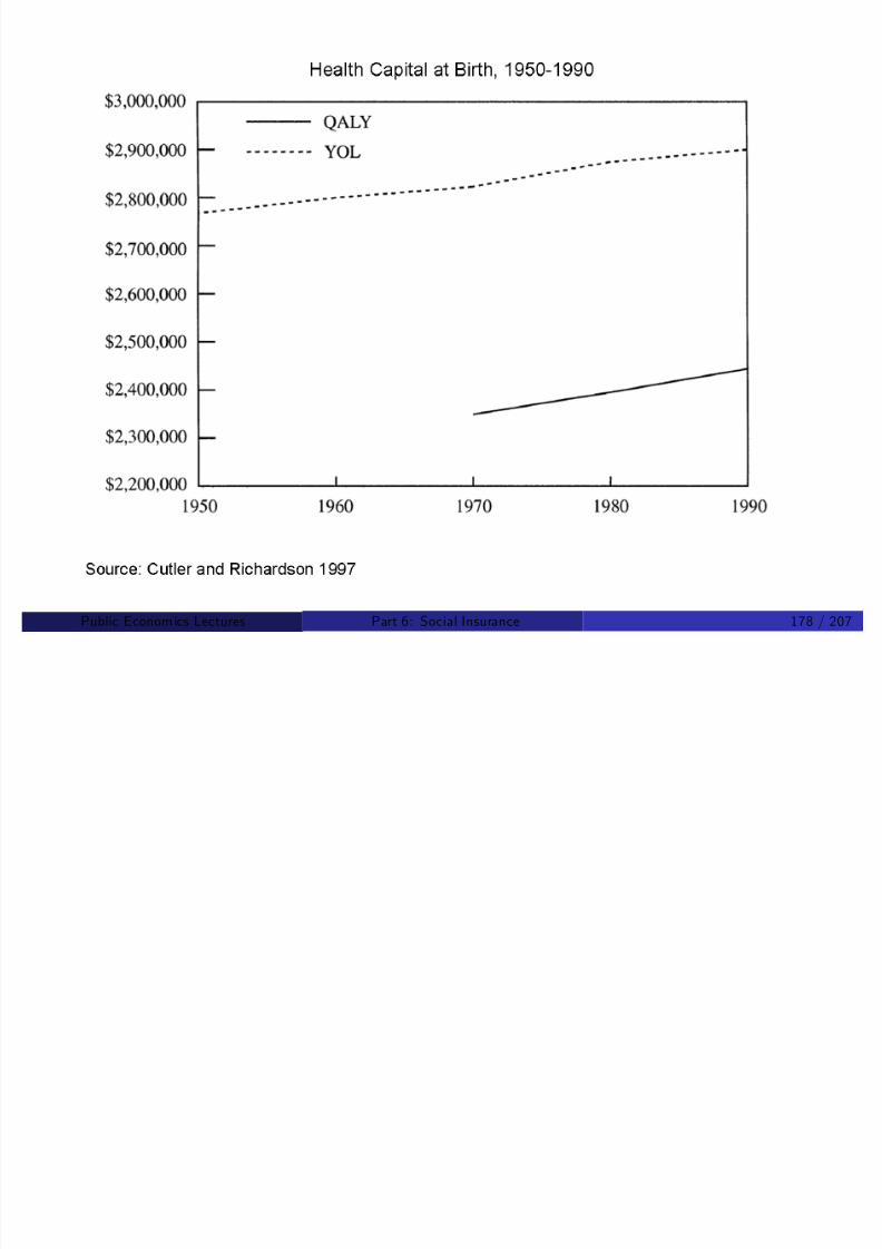
8/8/2019 Chetty - Public Economics Lectures
http://slidepdf.com/reader/full/chetty-public-economics-lectures 784/949
uestion: can we do even better b chan in overnment olicies?Public Econom ics Lectures () Part 6: Social Insurance 179 / 207
Optimal Govt. Intervention in Health Insurance
Now consider optimal design of government health insurance policies
Di¤erences relative to other social insurance programs:
1 Importance of provider side incentives.
2 Interaction between private and public insurance (crowdout).
Begin with a pure demand side model and then consider supply side.
Public Econom ics Lectures ()
Part 6: Social Insurance 180 / 207

8/8/2019 Chetty - Public Economics Lectures
http://slidepdf.com/reader/full/chetty-public-economics-lectures 785/949
Public Econom ics Lectures () Part 6: Social Insurance 180 / 207
Demand for Medical Care: Feldstein 1973
Price of medical care is 1, total wealth of consumer is y
s = smooth index of disease severity
m = amount of medical care purchased
c (m) = patient’s co-payment as a function of m
π = insurance premium
Public Econom ics Lectures ()
Part 6: Social Insurance 181 / 207

8/8/2019 Chetty - Public Economics Lectures
http://slidepdf.com/reader/full/chetty-public-economics-lectures 786/949
Public Econom ics Lectures () Part 6: Social Insurance 181 / 207
Feldstein 1973
x = non-medical consumption
H (s ,
m) = health as a fn. of disease state and medical care.
Assume H is concave in m
Let U (x , H ) = utility over the two goods
Public Econom ics Lectures ()
Part 6: Social Insurance 182 / 207

8/8/2019 Chetty - Public Economics Lectures
http://slidepdf.com/reader/full/chetty-public-economics-lectures 787/949
Public Econom ics Lectures () Part 6: Social Insurance 182 / 207
Feldstein 1973
Insurer sets premium to cover costs in expectation:
π =Z
[m(s ) c (m(s ))]f (s )ds
Individual chooses level of medical care by maximizing utility, takingπ as given
maxm(s )
Z [U (y π c (m(s )), H (s , m(s ))]f (s )ds
At an interior solution, individual will set 8s :
H m = c 0(m)U X
U H
Public Econom ics Lectures ()
Part 6: Social Insurance 183 / 207

8/8/2019 Chetty - Public Economics Lectures
http://slidepdf.com/reader/full/chetty-public-economics-lectures 788/949
Public Econom ics Lectures () Part 6: Social Insurance 183 / 207
Feldstein 1973: First Best Solution
Individual internalizes costs to insurer, so choose m based onc 0(m) = 1:
H m (m) =U X
U H
Optimal copayment is zero in all states
Note: this assumes that marginal utility of consumption is indepenentof health state
In general case, optimal to set MU sick = MU healthy , in which casecopayment may be desirable.
Public Econom ics Lectures ()
Part 6: Social Insurance 184 / 207

8/8/2019 Chetty - Public Economics Lectures
http://slidepdf.com/reader/full/chetty-public-economics-lectures 789/949
() /
Feldstein 1973: Second Best
In second best, individual only internalizes copayment
Consumes more medical care, because c 0(m) < 1 and H is concave
Resulting deadweight loss from insurance is analogous to that causedby overconsumption of a good because of a subsidy.
Optimal copay rate can be determined using tools analogous to thatin optimal UI model
Tradeo¤ between risk and moral hazard
Public Econom ics Lectures ()
Part 6: Social Insurance 185 / 207

8/8/2019 Chetty - Public Economics Lectures
http://slidepdf.com/reader/full/chetty-public-economics-lectures 790/949
() /
S=MC
D
Q1
Price
of each
visit
$200
Q2
A B
C
Number of
Doctor’s Visits
$100
Public Econom ics Lectures ()
Part 6: Social Insurance 186 / 207

8/8/2019 Chetty - Public Economics Lectures
http://slidepdf.com/reader/full/chetty-public-economics-lectures 791/949
Empirical Evidence: Moral Hazard in Health Insurance
Feldstein (1973): used cross-state variation to estimate an elasticity
of demand for medical care w.r.t price of 0.5.
Rich subsequent literature has yielded a variety of estimates.
Manning et al (1987): gold standard estimate based on $136 million
RAND experiment
Total sample: 6000.
Randomly assigned into 14 di¤erent ins. plans that varied in copay rate
Copay rate: was 0, 25, 50, or 95.
Tracked on average over 3 years, with full details on medical expenses.
Elasticity of about 0.1 for inpatient care, 0.2 for outpatient care
Public Econom ics Lectures ()
Part 6: Social Insurance 187 / 207

8/8/2019 Chetty - Public Economics Lectures
http://slidepdf.com/reader/full/chetty-public-economics-lectures 792/949
Public Econom ics Lectures ()
Part 6: Social Insurance 188 / 207

8/8/2019 Chetty - Public Economics Lectures
http://slidepdf.com/reader/full/chetty-public-economics-lectures 793/949
Finkelstein 2006
General equilibrium e¤ects may lead to much larger elasticities of consumption with respect to health insurance in equilibrium
Market-wide changes in demand alter hospitals’ practice styles andtechnology
Examines 1965 introduction of Medicare
Identi…cation strategy: geographic variation in ins. coverage prior to
1965
In northeast, 50% of elderly were insured, in south, 12% were insured
Public Econom ics Lectures ()
Part 6: Social Insurance 189 / 207

8/8/2019 Chetty - Public Economics Lectures
http://slidepdf.com/reader/full/chetty-public-economics-lectures 794/949Public Econom ics Lectures () Part 6: Social Insurance 190 / 207

8/8/2019 Chetty - Public Economics Lectures
http://slidepdf.com/reader/full/chetty-public-economics-lectures 795/949Public Econom ics Lectures () Part 6: Social Insurance 191 / 207

8/8/2019 Chetty - Public Economics Lectures
http://slidepdf.com/reader/full/chetty-public-economics-lectures 796/949
Finkelstein 2006
Impact of Medicare on hospital spending is six times larger thanpredicted by individual-level changes in RAND experiment
Estimates imply that increased health insurance can explain half of increase in health spending between 1950 and 1990
No direct normative implications: could be a liquidity or moral hazard
e¤ect.
Public Econom ics Lectures () Part 6: Social Insurance 192 / 207

8/8/2019 Chetty - Public Economics Lectures
http://slidepdf.com/reader/full/chetty-public-economics-lectures 797/949
Implications of Demand Side Model
Optimal insurance structure: deductible coupled with lower copay asshocks become large
Many policies look like this but not Medicare Part D
0% of the drug costs up to $250
75% of the costs for the next $2,250
0% of the costs for the next $3,600
95% of the costs above $5,100
Public Econom ics Lectures () Part 6: Social Insurance 193 / 207
8/8/2019 Chetty - Public Economics Lectures
http://slidepdf.com/reader/full/chetty-public-economics-lectures 798/949
Ellis and McGuire 1986
Previous analysis assumed a passive doctor.
In practice, physicians rather than patients likely to choose m
When physicians choose level of m, physician compensation schemedetermines e¢ciency of m
High copayments for patients may not solve the problem
Anecdotal evidence: dentists pulling out excess wisdom teeth
Public Econom ics Lectures () Part 6: Social Insurance 194 / 207

8/8/2019 Chetty - Public Economics Lectures
http://slidepdf.com/reader/full/chetty-public-economics-lectures 799/949
Ellis and McGuire 1986: Setup
Goal: contrast e¢ciency of payment systems for physicians andanalyze optimal system
Payment for physician services is
P = α + βc
α =…xed cost payment for practice
β =payment for proportional costs (tests, nurses)
Public Econom ics Lectures () Part 6: Social Insurance 195 / 207
8/8/2019 Chetty - Public Economics Lectures
http://slidepdf.com/reader/full/chetty-public-economics-lectures 800/949
Ellis and McGuire: Compensation Schemes
Various methods of payment (α, β):
1 Fee-for-service [α = 0, β > 1]: No …xed payment for practice, butinsurance company pays full cost of all visits to doctor + a surcharge.
2 Salary [α > 0, β = 1]: practice costs paid for as well as marginal costsof treatment.
3 Capitation [α > 0, β = 0]: varying by type and # of patient but not
services rendered
Public Econom ics Lectures () Part 6: Social Insurance 196 / 207
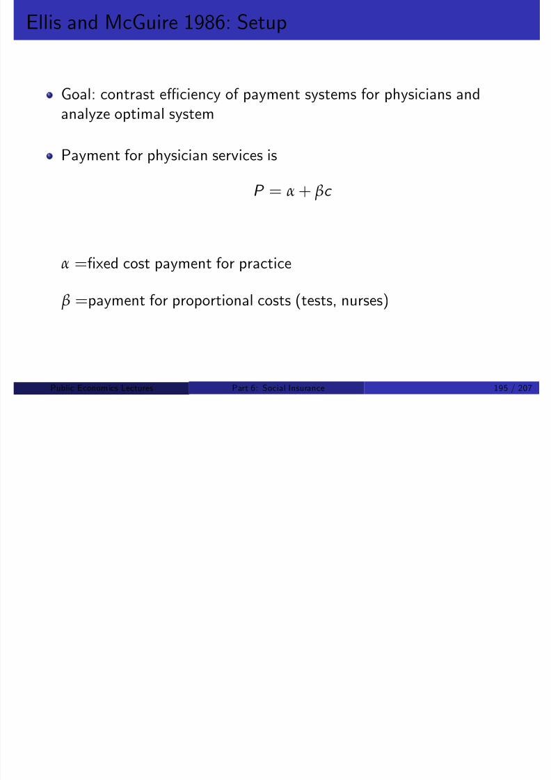
8/8/2019 Chetty - Public Economics Lectures
http://slidepdf.com/reader/full/chetty-public-economics-lectures 801/949
Ellis and McGuire: Compensation Schemes
General trend has been toward higher α, lower β
Private market has shifted from FFS to HMO capitation schemes
Medicare/Medicaid shifted in ‘80s to a prospective payment scheme
Tradeo¤: lower β provides incentives for doctors to provide lessservices. But they may provide too little!
Lower costs, but complaints of lower quality of care
Public Econom ics Lectures () Part 6: Social Insurance 197 / 207

8/8/2019 Chetty - Public Economics Lectures
http://slidepdf.com/reader/full/chetty-public-economics-lectures 802/949
Ellis and McGuire: Optimal Payment Scheme
To characterize optimal payment scheme, need to specify howphysician chooses quality of care
Physician’s utility function:
U = θπ + (1 θ)q
π =pro…ts earned by physician
q =quality of care = bene…t to patient.
With payment scheme (α, β), pro…ts are
π = α + βc (q ) c (q )
Public Econom ics Lectures () Part 6: Social Insurance 198 / 207

8/8/2019 Chetty - Public Economics Lectures
http://slidepdf.com/reader/full/chetty-public-economics-lectures 803/949
Ellis and McGuire: Optimal Payment Scheme
Doctors solve
maxq
θ(α + βc (q ) c (q )) + (1 θ)q
Society’s problem is to maximize quality of care net of costs
maxq
q c (q )
Socially optimal quality level: q such that
c 0(q ) = 1
Public Econom ics Lectures () Part 6: Social Insurance 199 / 207

8/8/2019 Chetty - Public Economics Lectures
http://slidepdf.com/reader/full/chetty-public-economics-lectures 804/949
Ellis and McGuire: Optimal Payment Scheme
The level of care q D provided by doctor is such that:
dU dq
= θ( β 1)c 0(q D ) θ + 1 = 0
) c 0(q D ) =1 θ
θ(1 β)
So, in order to get the doctor to choose the social optimum, need toset β such that q D = q .
1 = c 0(q ) = c 0(q D
) =
1
θ
θ(1 β)
) β = 2 1
θ
Public Econom ics Lectures () Part 6: Social Insurance 200 / 207

8/8/2019 Chetty - Public Economics Lectures
http://slidepdf.com/reader/full/chetty-public-economics-lectures 805/949
Ellis and McGuire: Optimal Payment Scheme
β = 2
1
θOptimal degree of incentive pay is increasing in θ.
Intuition: if doctor is sel…sh (high θ), reimburse him for costs of
provision so that he doesn’t under-provide service to patients.
But if he is benevolent, reduce the amount he gets paid for provision.
He will naturally get bene…ts from taking care of them and will
over-provide if he is paid for it too.
HMOs desirable if healthcare providers are benevolent; FFSreimbursement if they are pro…t-seeking.
Public Econom ics Lectures () Part 6: Social Insurance 201 / 207

8/8/2019 Chetty - Public Economics Lectures
http://slidepdf.com/reader/full/chetty-public-economics-lectures 806/949
Ellis and McGuire Model: Limitations
Ignores cream-skimming by doctors if they must bear costs
Doctors assumed to be risk neutral
Static model: ignores technological change and incentives to innovate
Finkelstein (2004): policies intended to change utilization of vaccinesled to more innovation, some of which may have been unproductive
Would be useful to derive an empirically implementable formula for β
Ex: use doctors’ treatment of themselves or kids/relatives
Public Econom ics Lectures () Part 6: Social Insurance 202 / 207
E i i l E id S l Sid I i

8/8/2019 Chetty - Public Economics Lectures
http://slidepdf.com/reader/full/chetty-public-economics-lectures 807/949
Empirical Evidence on Supply Side Incentives
Cutler (1995) examines mortality and readmission outcomes around1983 Medicare reform.
Finds an e¤ect on timing of death, but no e¤ect in long run.
Suggests that physicians were practicing “‡at of the curve” medicine.
Physicians may be benevolent enough that a capitation scheme isoptimal.
Public Econom ics Lectures () Part 6: Social Insurance 203 / 207
C d f P i I

8/8/2019 Chetty - Public Economics Lectures
http://slidepdf.com/reader/full/chetty-public-economics-lectures 808/949
Crowdout of Private Insurance
So far have assumed a single insurer. In practice, both private and
public ins. coexist.
To what extent does crowdout of other insurance mechanismsdiminish bene…ts of government intervention?
Cutler and Gruber (1996): Medicaid crowdout
Medicaid expansions to pregnant mothers di¤erent across states
50% of added Medicaid enrollment came from dropping private healthins. coverage through employer.
Chetty and Saez (2008): optimal insurance with crowdout of privatesector insurance contracts
Public Econom ics Lectures () Part 6: Social Insurance 204 / 207
C i d G b 1995 B … f P bli I

8/8/2019 Chetty - Public Economics Lectures
http://slidepdf.com/reader/full/chetty-public-economics-lectures 809/949
Currie and Gruber 1995: Bene…ts of Public Insurance
(1) (2) (3)
A: Variation by State: Eligibility for Children
Year Missouri eligibility Michigan eligibility
1982 12% 20%
2000 76% 34%
B. Variation by age: Eligibility in Washington D.C.
Year Age 14 eligibility Age 0 eligibility
1982 18% 48%
2000 59% 56%
Source: Gruber 2007
Medicaid Eligibility Changes
Public Econom ics Lectures () Part 6: Social Insurance 205 / 207
C i d G b 1995 B …t f P bli I

8/8/2019 Chetty - Public Economics Lectures
http://slidepdf.com/reader/full/chetty-public-economics-lectures 810/949
Currie and Gruber 1995: Bene…ts of Public Insurance
30 pp increase in Medicaid eligibility among 15-44 year old moms hastwo e¤ects
Greater utilization: early prenatal care visits rose by more than 50%.
Better health outcomes: infant mortality declined by 8.5% due to theexpansions in Medicaid for pregnant women.
Bene…cial e¤ects large because this is likely to be an underinsured,underserved population
Public Econom ics Lectures () Part 6: Social Insurance 206 / 207
Costs Per Life Saved of Various Regulations
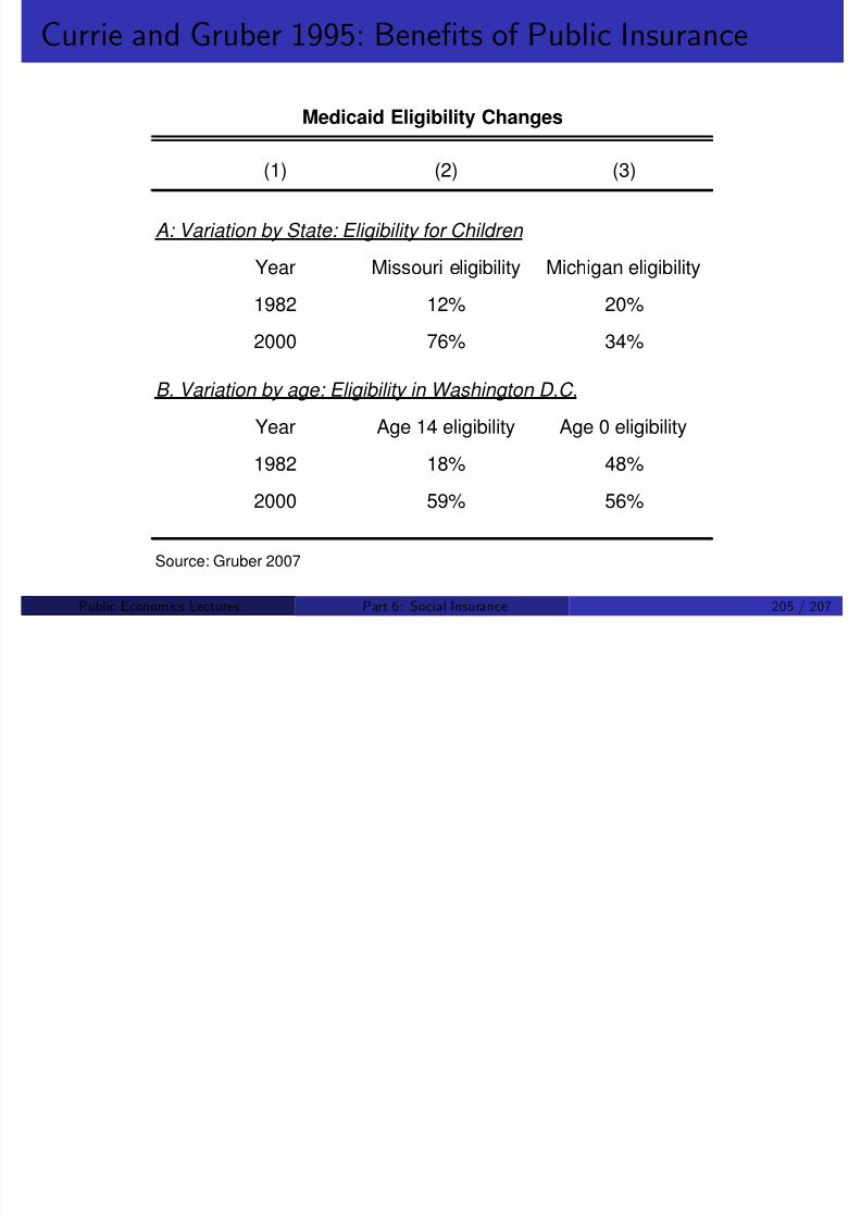
8/8/2019 Chetty - Public Economics Lectures
http://slidepdf.com/reader/full/chetty-public-economics-lectures 811/949
Regulation concerning … Year Agency
Cost per lifesaved ($millions)
• Childproof lighters 1993 CPSC $0.10
• Food labeling 1993 FDA 0.4
• Reflective devices for heavy trucks 1999 NHTSA 0.9
Medicaid pregnancy expansions 1996 Currie and Gruber 1
• Children’s sleepware flammability 1973 CPSC 2.2
• Rear/up/shoulder seatbelts in cars 1989 NHTSA 4.4
• Asbestos 1972 OSHA 5.5
Value of statistical life 7
• Benezene 1987 OSHA 22
• Asbestos ban 1989 EPA 78
• Cattle feed 1979 FDA 170
• Solid waste disposal facilities 1991 EPA 100,000
Source: Gruber 2007
Costs Per Life Saved of Various Regulations
Public Econom ics Lectures () Part 6: Social Insurance 207 / 207

8/8/2019 Chetty - Public Economics Lectures
http://slidepdf.com/reader/full/chetty-public-economics-lectures 812/949
Public Economics LecturesPart 7: Public Goods and Externalities
Raj Chetty and Gregory A. Bruich
Harvard UniversityFall 2009
Public Economics Lectures () Part 7: Public Goods and Externalities 1 / 138
Public Goods: Outline

8/8/2019 Chetty - Public Economics Lectures
http://slidepdf.com/reader/full/chetty-public-economics-lectures 813/949
Public Goods: Outline
1 De…nitions and Baseline Model
2 Samuelson Rule
3 Lindahl Pricing
4 Social Choice: Median Voter Theorem
5 Public Goods with Endogenous Private Provision
6 Public Goods with Distortionary Taxation
7 Charity and Private Provision
Public Economics Lectures () Part 7: Public Goods and Externalities 2 / 138
Public vs Private Goods
8/8/2019 Chetty - Public Economics Lectures
http://slidepdf.com/reader/full/chetty-public-economics-lectures 814/949
Public vs. Private Goods
Private goods bene…t one individual h
∑ h
X h X
Public goods bene…t several individuals simultaneously
X h X 8h
Ex: can of coke vs. teaching a class
Pure: can accommodate any number of users.
Impure: subject to congestion
radio vs. roads
Public Economics Lectures () Part 7: Public Goods and Externalities 3 / 138

8/8/2019 Chetty - Public Economics Lectures
http://slidepdf.com/reader/full/chetty-public-economics-lectures 815/949
Private Good
Person 1’sConsumption
Person 2’s Consumption
Public Economics Lectures () Part 7: Public Goods and Externalities 4 / 138

8/8/2019 Chetty - Public Economics Lectures
http://slidepdf.com/reader/full/chetty-public-economics-lectures 816/949
Public Good
Person 1’sConsumption
Person 2’s Consumption
Public Economics Lectures () Part 7: Public Goods and Externalities 5 / 138
Public vs Private Goods

8/8/2019 Chetty - Public Economics Lectures
http://slidepdf.com/reader/full/chetty-public-economics-lectures 817/949
Public vs. Private Goods
Rival vs. non-rival.
Pure are non-rival
Excludable vs. non-excludable.
National Radio: impossible to exclude. Teaching: possible to exclude
Most economic analysis focuses on pure public goods
Public goods ) equilibrium outcome ine¢cient (large scaleproduction externalities)
Public Economics Lectures () Part 7: Public Goods and Externalities 6 / 138
Public Goods Model: Setup

8/8/2019 Chetty - Public Economics Lectures
http://slidepdf.com/reader/full/chetty-public-economics-lectures 818/949
Public Goods Model: Setup
Economy with H households, indexed by h = 1, . ., H
Two goods X and G
X is always private, individual h consumes quantity X
h
Denote by X = ∑ h X h the total quantity of good X in the economy
Denote by G h consumption of good G by h, with G = ∑ h G h
Utility of h is U h = U h(X h, G h)
Public Economics Lectures () Part 7: Public Goods and Externalities 7 / 138
Public Goods Model: Setup

8/8/2019 Chetty - Public Economics Lectures
http://slidepdf.com/reader/full/chetty-public-economics-lectures 819/949
Public Goods Model: Setup
Social welfare = weighted sum of utilities, βh weight on h
βh 0 and at least one βh > 0
Production possibility F (X , G ) = 0
Assume that U h is increasing in X and G
Public Economics Lectures () Part 7: Public Goods and Externalities 8 / 138
First Best if G is Private
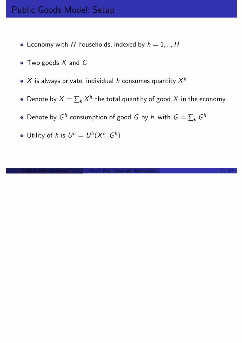
8/8/2019 Chetty - Public Economics Lectures
http://slidepdf.com/reader/full/chetty-public-economics-lectures 820/949
First Best if G is Private
To identify Pareto e¢cient outcomes, solve:
max∑ h
βhU h(X h , G h)
s.t. F (∑ h
X h ,∑ h
G h) 0 [λ]
Equivalent to maxU 1 s.t. U h U h0 for all h 0 and F 0.Lagrangian:
L = ∑ βhU h λF
First order conditions
[X h ] : βhU hX = λF X
[G h ] : βhU hG = λF G
Public Economics Lectures () Part 7: Public Goods and Externalities 9 / 138
First Best if G is Private
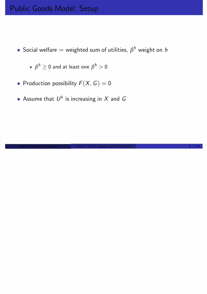
8/8/2019 Chetty - Public Economics Lectures
http://slidepdf.com/reader/full/chetty-public-economics-lectures 821/949
First Best if G is Private
Taking ratios of FOCs yields
U hG U hX
=F G
F X
Set of Pareto e¢cient allocations is set of allocations that satisfy:
MRS hGX = MRT GX 8h
Decentralized market equilibrium will implement such an allocation(1st Welfare Thm).
Public Economics Lectures () Part 7: Public Goods and Externalities 10 / 138

8/8/2019 Chetty - Public Economics Lectures
http://slidepdf.com/reader/full/chetty-public-economics-lectures 822/949
First Best if G is a Pure Public Good
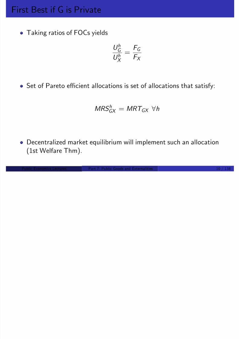
8/8/2019 Chetty - Public Economics Lectures
http://slidepdf.com/reader/full/chetty-public-economics-lectures 823/949
To identify Pareto e¢cient outcomes,
max∑ h βhU h(X h , G )
s.t. F (∑ h
X h ,∑ h
G h) 0 [λ]
FOC’s:
[X h ] : βhU hX = λF X
[G ] : ∑ h
βhU hG = λF G
Using βh = λF X /U hX from f.o.c. for X h we obtain:
∑ h
[U hG U hX
] =F G
F X
Public Economics Lectures () Part 7: Public Goods and Externalities 12 / 138
Samuelson (1954) Rule

8/8/2019 Chetty - Public Economics Lectures
http://slidepdf.com/reader/full/chetty-public-economics-lectures 824/949
( )
Condition for Pareto e¢ciency: sum of MRS is equal to MRT:
∑ h
MRS hGX = MRT GX
Intuition: an additional unit of G increases the utility of allhouseholds in the public good case
With G a private good, an additional unit only increases oneindividual’s utility
Public Economics Lectures () Part 7: Public Goods and Externalities 13 / 138
Samuelson (1954) Rule
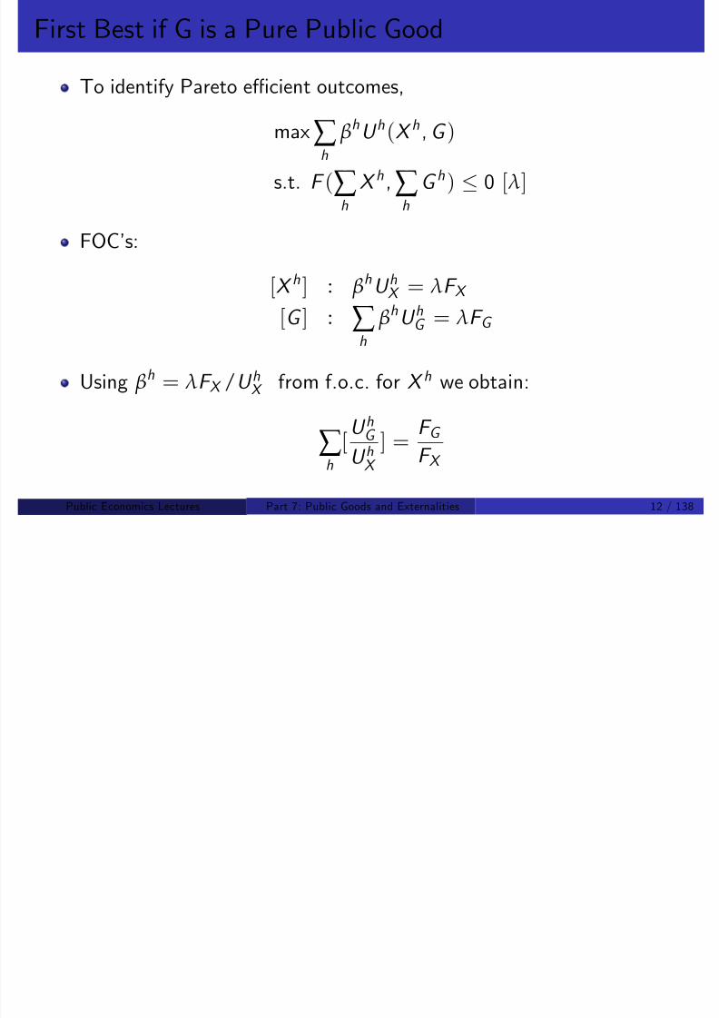
8/8/2019 Chetty - Public Economics Lectures
http://slidepdf.com/reader/full/chetty-public-economics-lectures 825/949
( )
Excludability plays no role in the analysis.
Only relevant for determining feasible provision mechanisms
Samuelson rule simple but di¢cult to implement in practice.
Govt needs to know preferences
Issue of how to …nance the public good
Samuelson analysis is a …rst-best benchmark
How can optimal level of PG be implemented with available policytools?
Public Economics Lectures () Part 7: Public Goods and Externalities 14 / 138
Model of Private Provision: Setup

8/8/2019 Chetty - Public Economics Lectures
http://slidepdf.com/reader/full/chetty-public-economics-lectures 826/949
Private good X and a pure public good G .
Price of each good is normalized to one (one-to-one transformationtechnology).
Each household starts with an endowment Y h of good X .
Individual h contributes G h to public good funding.
Consumption of public good is G = ∑ h G
h
for everyone.
Consumption of the private good is X h = Y h G h for individual h.
Public Economics Lectures () Part 7: Public Goods and Externalities 15 / 138
Decentralized Private Provision Suboptimal

8/8/2019 Chetty - Public Economics Lectures
http://slidepdf.com/reader/full/chetty-public-economics-lectures 827/949
Individual h solves
maxU h(X h, G 1 + .. + G h + .. + G H )
s.t. X h + G h = Y h .
Nash equilibrium outcome is U hX = U hG
Samuelson Rule not satis…ed
Pareto improvement if each person invested 1/H more dollars in thepublic good:
∆W = U hX (1/H ) + U hG = U hG (1 1/H ) > 0.
Market outcome is ine¢cient; underprovision of G
Public Economics Lectures () Part 7: Public Goods and Externalities 16 / 138
Lindahl Equilibrium
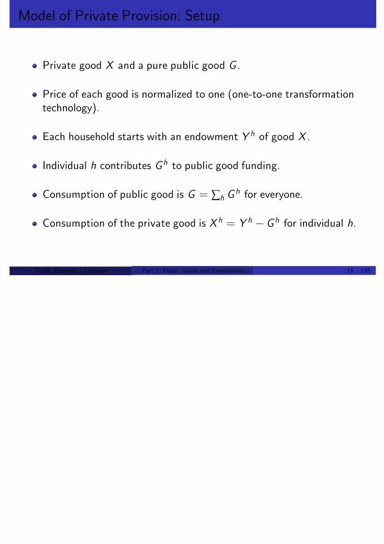
8/8/2019 Chetty - Public Economics Lectures
http://slidepdf.com/reader/full/chetty-public-economics-lectures 828/949
How to achieve Pareto e¢ciency through a decentralized mechanism?
Suppose individual h has to pay a share τ h of the public good andcan pick a level of G
Individual h chooses G to maximize
U h(Y h τ hG , G )
FOC: τ hU hX = U hG .
Demand function of G h = G h(τ h, Y h)
Public Economics Lectures () Part 7: Public Goods and Externalities 17 / 138
Lindahl Equilibria: Conditions
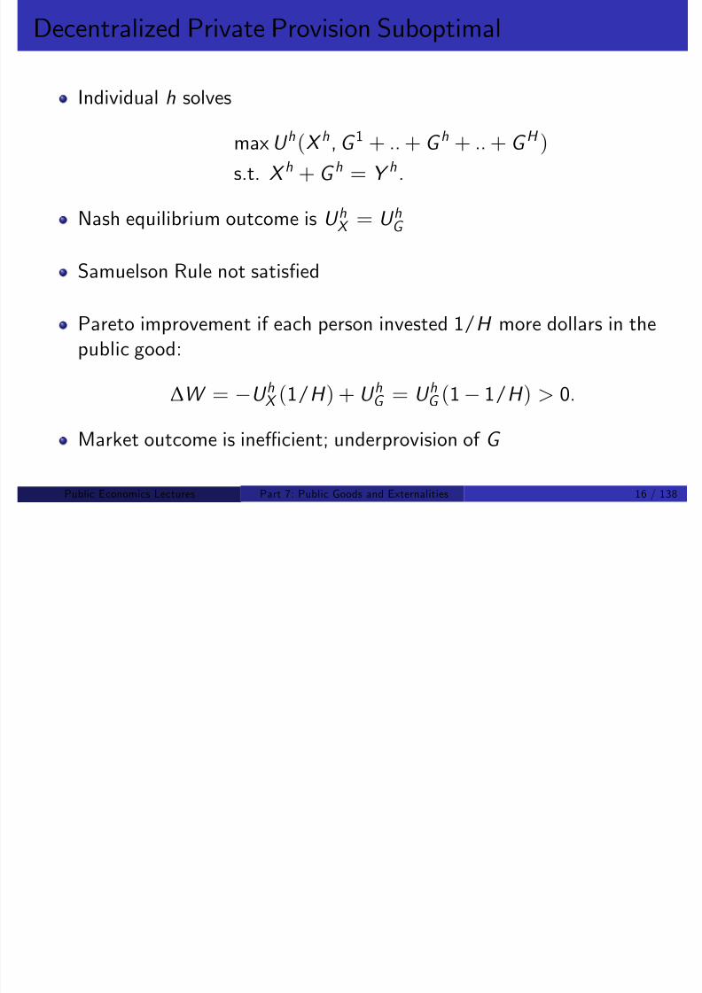
8/8/2019 Chetty - Public Economics Lectures
http://slidepdf.com/reader/full/chetty-public-economics-lectures 829/949
A Lindahl Equilibrium satis…es the following two conditions:
1 Public good must be fully …nanced.
∑ h
τ h = 1
2 All individuals must demand same quantity of G .
Lindahl equilibrium generically exists: H equations (G 1 = ... = G H and ∑ h τ
h = 1) and H unknowns (τ h)
Public Economics Lectures () Part 7: Public Goods and Externalities 18 / 138
Lindahl Equilibria: Key Properties (Foley 1970)
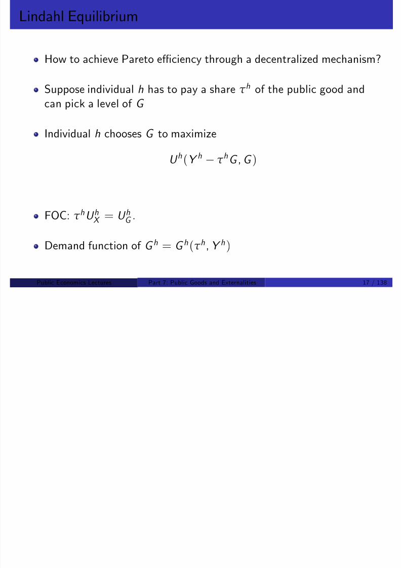
8/8/2019 Chetty - Public Economics Lectures
http://slidepdf.com/reader/full/chetty-public-economics-lectures 830/949
Samuelson Rule applies and outcome is Pareto e¢cient:
∑ h
[U hG U hX
] = ∑ h
τ h = 1
With identical individuals, simply set tax τ = 1H
and ask individualsto voluntarily contribute to G
With heterogeneity, e¢cient outcome can be attained with public
goods through prices that are individual-speci…c
Public Economics Lectures () Part 7: Public Goods and Externalities 19 / 138
Lindahl Pricing: Practical Constraints

8/8/2019 Chetty - Public Economics Lectures
http://slidepdf.com/reader/full/chetty-public-economics-lectures 831/949
1 Must be able to exclude a consumer from using the public good.
Does not work with non-excludable public good
2 Must know individual preferences to set personalized prices τ h
Agents have no incentives to reveal their preferences
Di¤erence between Lindahl equilibria and standard equilibria:
No decentralized mechanism for deriving prices; no market forces that
will generate the right price vector
So how do we actually determine level of PG’s in practice?
Voting on bundles of PG’s and taxesDoes voting lead to the …rst best solution?
Public Economics Lectures () Part 7: Public Goods and Externalities 20 / 138
Voting Model: Setup

8/8/2019 Chetty - Public Economics Lectures
http://slidepdf.com/reader/full/chetty-public-economics-lectures 832/949
Suppose that public good is …nanced by …xed taxes τ hG
Individuals vote on G but not on τ h
Preferences over G given by U h(Y h τ hG , G )
Voting equilibrium: level G eq of public that cannot be defeated inmajority rule by any other alternative G
Condorcet Paradox: majority voting does not lead to a stable outcome
Consider voting on public school spending by 3 parents (low, middle,and high income)
Public Economics Lectures () Part 7: Public Goods and Externalities 21 / 138

8/8/2019 Chetty - Public Economics Lectures
http://slidepdf.com/reader/full/chetty-public-economics-lectures 833/949
Condorcet Paradox
Individual
1 2 3
1st H M L
2nd M L H
3rd L H M
Preference
Ordering
Cycling in social ordering: H > M > L > H
Public Economics Lectures () Part 7: Public Goods and Externalities 22 / 138
Arrow (1951) and Single-Peaked Preferences

8/8/2019 Chetty - Public Economics Lectures
http://slidepdf.com/reader/full/chetty-public-economics-lectures 834/949
Arrow’s Impossibility Thm: Condorect Paradox is a general problem
Only social choice rule that satis…es (a) Pareto E¢ciency and (b)Independence of Irrelevant Alternatives is dictatorship.
Subsequent work: restricts space of preferences to make progress
Two assumptions that ensure existence of equilibrium:
1
G unidimensional
2 preferences over G are “single-peaked”
Public Economics Lectures () Part 7: Public Goods and Externalities 23 / 138
Single-Peaked Preferences
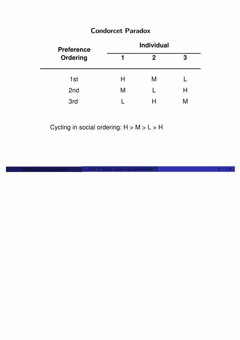
8/8/2019 Chetty - Public Economics Lectures
http://slidepdf.com/reader/full/chetty-public-economics-lectures 835/949
1
1 . 5
2
2 . 5
3
P r e f e r e n c
e O r d e r i n g ( U t i l i t y
)
Low Medium High
Level of Public Spending
Person 1 Person 2 Person 3
Public Economics Lectures () Part 7: Public Goods and Externalities 24 / 138
Median Voter Theorem

8/8/2019 Chetty - Public Economics Lectures
http://slidepdf.com/reader/full/chetty-public-economics-lectures 836/949
With single-peaked preferences, majority voting rule produces a votingequilibrium (stable choice)
Voting eq. is characterized by preferred level of voter whose preferred
level of PG spending is at the median of the distribution
Compute preferred spending for each individual, G h
Majority voting will select median of distribution of G h
Public Economics Lectures () Part 7: Public Goods and Externalities 25 / 138
Median Voter Theorem

8/8/2019 Chetty - Public Economics Lectures
http://slidepdf.com/reader/full/chetty-public-economics-lectures 837/949
Median Voter Theorem
D e n s i t y
School Spending
Equilibrium:Median Pref.
Public Economics Lectures () Part 7: Public Goods and Externalities 26 / 138
Median Voter Choice: E¢ciency

8/8/2019 Chetty - Public Economics Lectures
http://slidepdf.com/reader/full/chetty-public-economics-lectures 838/949
In general, median voter equilibrium is not Pareto e¢cient:
Suppose τ h = 1/H for all h
Voting outcome: MRS (G med ) = 1/H .
Samuelson rule: ∑ h MRS (G h)/H = 1/H
Di¤erence between median and mean determines degree of ine¢ciency
Potential rationale for permitting lobbying to express intensity of preferences
Public Economics Lectures () Part 7: Public Goods and Externalities 27 / 138
Lee, Moretti, and Butler 2004

8/8/2019 Chetty - Public Economics Lectures
http://slidepdf.com/reader/full/chetty-public-economics-lectures 839/949
In practice, citizens do not vote on every bill; elect representatives todo so.
In a standard (Hotelling) model, median voter theorem predicts thatcandidates will implement median voter’s preferences when elected
Move toward center to win election
Lee et al: does this happen in practice?
Use “close” elections as experiments in an RD design
Public Economics Lectures () Part 7: Public Goods and Externalities 28 / 138
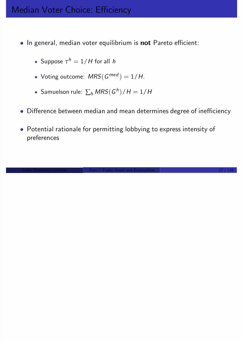
8/8/2019 Chetty - Public Economics Lectures
http://slidepdf.com/reader/full/chetty-public-economics-lectures 840/949
Public Economics Lectures () Part 7: Public Goods and Externalities 29 / 138
Lee, Moretti, and Butler 2004

8/8/2019 Chetty - Public Economics Lectures
http://slidepdf.com/reader/full/chetty-public-economics-lectures 841/949
Evidence on Congressional voting sharply contradicts prediction of median voter theory
Politicians’ inability to credibly commit to a compromise dominatescompetition-induced convergence in policy.
For example, a large exogenous increase in electoral strength for theDemocratic party in a district does not result in shifting both parties’nominees to the left.
Cannot rely on median voter logic to implement e¢cient choice even
if mean and median are close
Need to devise social choice mechanisms that account forcommitment problems
Public Economics Lectures () Part 7: Public Goods and Externalities 30 / 138
Optimal Second Best Provision of PG’s
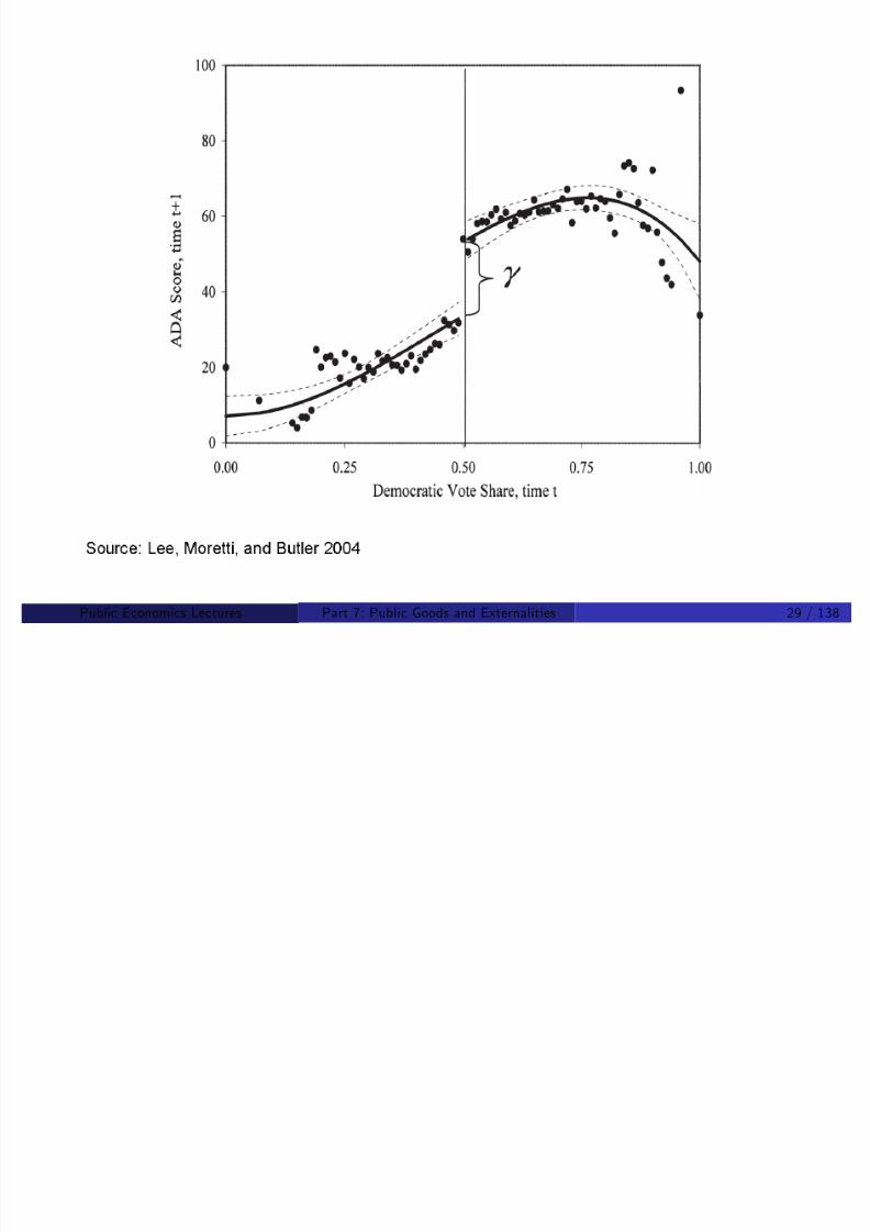
8/8/2019 Chetty - Public Economics Lectures
http://slidepdf.com/reader/full/chetty-public-economics-lectures 842/949
Suppose govt has decided to levy a tax and provide public goods
based on some rule
Two complications arise when trying to get to Samuelson First Bestlevel:
1 Interactions with private sector provision (crowdout).
Andreoni (2007): $250B/yr in private contributions.
2 Government cannot …nance PGs through lump sum taxation
Must modify Samuelson rule to account for distortionary taxation
Public Economics Lectures () Part 7: Public Goods and Externalities 31 / 138
Public Goods with Endogenous Private Provision
8/8/2019 Chetty - Public Economics Lectures
http://slidepdf.com/reader/full/chetty-public-economics-lectures 843/949
Interest in crowd-out began with Roberts (1984)
Expansion of govt services for poor since Great Depressionaccompanied by comparable decline in charitable giving for the poor.
Conclusion: government has grown tremendously without having anynet impact on poverty or welfare
Evidence mainly based on time series impressions.
But theory underlying this claim very sensible, as subsequent workshowed
Public Economics Lectures () Part 7: Public Goods and Externalities 32 / 138
Bergstrom, Blume, and Varian (1986): Setup

8/8/2019 Chetty - Public Economics Lectures
http://slidepdf.com/reader/full/chetty-public-economics-lectures 844/949
Individual h solves:
maxX h ,G h
U h(X h, G h + G h )
s.t. X h + G h = Y h
FOC is U hX = U
hG
Nash equilibrium exists and is unique
G s.t. all individuals optimize given others’ behavior
Let G denote private equilibrium outcome
Public Economics Lectures () Part 7: Public Goods and Externalities 33 / 138
Bergstrom-Blume-Varian Model: Crowd-out

8/8/2019 Chetty - Public Economics Lectures
http://slidepdf.com/reader/full/chetty-public-economics-lectures 845/949
Now suppose government introduces lump sum taxes t h on eachindividual h
Revenue used to …nance expenditure on public good T = ∑ t h
Individual’s optimization problem is now:
maxU (X h, G h + G h + T )
s.t. X h + G h = Y h t h
Public Economics Lectures () Part 7: Public Goods and Externalities 34 / 138
Bergstrom-Blume-Varian Model: Crowd-out
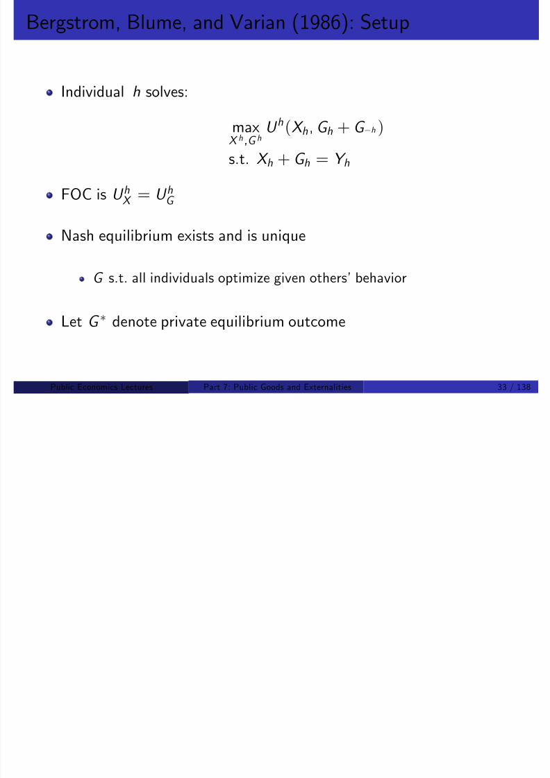
8/8/2019 Chetty - Public Economics Lectures
http://slidepdf.com/reader/full/chetty-public-economics-lectures 846/949
LetZ h =
G h +
t h denote total contribution of individual
h.
Can rewrite this as:
maxU (X h, Z h + Z h)
s.t. X h + Z h = Y h
This is isomorphic to original problem ) Z = G
Total public good provision is unchanged!
Each person simply reduces voluntary provision by t h
Public Economics Lectures () Part 7: Public Goods and Externalities 35 / 138

8/8/2019 Chetty - Public Economics Lectures
http://slidepdf.com/reader/full/chetty-public-economics-lectures 847/949
Public Economics Lectures () Part 7: Public Goods and Externalities 36 / 138
BBV Model: Additional Results

8/8/2019 Chetty - Public Economics Lectures
http://slidepdf.com/reader/full/chetty-public-economics-lectures 848/949
1 Total supply of the public good is indep. of the distribution of incomeamong givers (Warr 1983)
Logic can be seen with two transfers.Tax indiv. 1 to …nance PG; then subsidize indiv. 2 and reduce PGexpenditure.Neither action has a real e¤ect by crowdout result.
2 When preferences are identical and separable in x and G , all givers toa public good will have the same level of private consumption in eq.regardless of their incomes (BBV 1986).
u 1
x (x ,
G ) = u 1
G (x ,
G ) = u 2
G (x ,
G ) = u 2
x (x ,
G )) x 1 = x 2
3 As size of economy gets large, the proportion of individuals who giveto the PG approaches zero (Andreoni 1988).
Public Economics Lectures () Part 7: Public Goods and Externalities 37 / 138
BBV Model: Key Assumptions
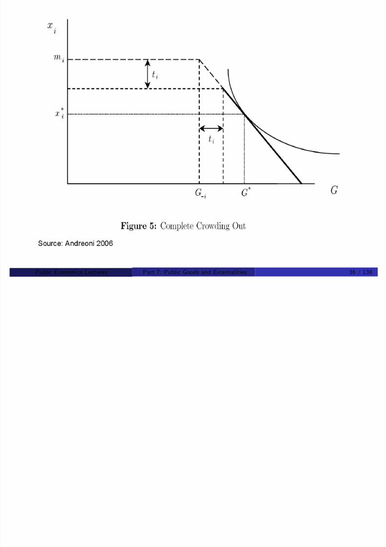
8/8/2019 Chetty - Public Economics Lectures
http://slidepdf.com/reader/full/chetty-public-economics-lectures 849/949
1 No corners: assumed the set of contributors are the same in bothsituations.
With corners, transfer neutrality breaks down: tax increase T results inno private contribution from individuals with G h < T , butcontributions increase on net.
2 Ignores direct utility from giving: U (X h,
G h,
G ).
Andreoni’s (1990) “warm glow” model.
Stigler and Becker (1977) critique: should not simply modify
preferences to explain patterns
3 Ignores prestige/signalling motives
Glazer and Konrad (1996)
Public Economics Lectures () Part 7: Public Goods and Externalities 38 / 138
Empirical Evidence on Crowd-Out

8/8/2019 Chetty - Public Economics Lectures
http://slidepdf.com/reader/full/chetty-public-economics-lectures 850/949
Two empirical questions motivated by theory
1 How large is the degree of crowd-out in practice?
2 What are the income and price e¤ects on charitable giving?
Two strands of empirical literature
1 Field evidence (observational studies)
2 Lab experiments
Traditionally, lab experiments have been more in‡uential but recent…eld studies may change this
Lab experiments may not capture important motives for giving: warmglow, prestige
Public Economics Lectures () Part 7: Public Goods and Externalities 39 / 138
Kingma 1989

8/8/2019 Chetty - Public Economics Lectures
http://slidepdf.com/reader/full/chetty-public-economics-lectures 851/949
Studies individual contributions to public radio stations
Cross-sectional survey of individuals who listened to public radio.3,500 individuals and 63 di¤erent radio stations.
Research Design: OLS regression of individual contributions on
government support
D i = β0 + β1G i + X i γ + i
D i = individual contribution
G i = government support
X i = set of controls: individual income, individual education, age,price (tax bracket).
Public Economics Lectures () Part 7: Public Goods and Externalities 40 / 138

8/8/2019 Chetty - Public Economics Lectures
http://slidepdf.com/reader/full/chetty-public-economics-lectures 852/949
Public Economics Lectures () Part 7: Public Goods and Externalities 41 / 138
Kingma 1989
M i l β 0 01 d f 20%

8/8/2019 Chetty - Public Economics Lectures
http://slidepdf.com/reader/full/chetty-public-economics-lectures 853/949
Main result: β1 = 0.015 –> crowd-out rate of 20%
Signi…cantly negative but much less than 1-1 prediction of theory
Problem: government support might depend on individualcontributions.
E.g. non-contribution by individuals leads to govt provision
Creates a spurious negative correlation between govt support andindividual contributions.
We need an exogenous “shifter” that a¤ects govt contributionwithout a¤ecting individual contributions.
E.g.: legislated reform that bans govt support.
Public Economics Lectures () Part 7: Public Goods and Externalities 42 / 138
Hungerman 2005

8/8/2019 Chetty - Public Economics Lectures
http://slidepdf.com/reader/full/chetty-public-economics-lectures 854/949
Studies crowdout of church-provided welfare (soup kitchens, etc.) bygovernment welfare.
Uses 1996 Clinton welfare reform act as an instrument for welfare
spending.
One aspect of reform: reduced/eliminated welfare for non-citizens.
Motivates a di¤-in-di¤ strategy: compare churches in high non-citizen
areas with low non-citizen areas before/after 1996 reform.
Public Economics Lectures () Part 7: Public Goods and Externalities 43 / 138

8/8/2019 Chetty - Public Economics Lectures
http://slidepdf.com/reader/full/chetty-public-economics-lectures 855/949
Public Economics Lectures () Part 7: Public Goods and Externalities 44 / 138
Hungerman 2005
8/8/2019 Chetty - Public Economics Lectures
http://slidepdf.com/reader/full/chetty-public-economics-lectures 856/949
Estimates imply that total church expenditures in a state go up by 40cents when welfare spending is cut by $1.
Exogenous variation make these estimates much more credible
Public Economics Lectures () Part 7: Public Goods and Externalities 45 / 138
Andreoni and Payne 2003

8/8/2019 Chetty - Public Economics Lectures
http://slidepdf.com/reader/full/chetty-public-economics-lectures 857/949
Government spending crowds-out private donations through twochannels: willingness to donate + fundraising
Use tax return data on arts and social service organizations
Panel study: includes organization and year …xed e¤ects
Public Economics Lectures () Part 7: Public Goods and Externalities 46 / 138
Andreoni and Payne 2003

8/8/2019 Chetty - Public Economics Lectures
http://slidepdf.com/reader/full/chetty-public-economics-lectures 858/949
OLS still yields “wrong signed” estimates:
More government spending ! more fundraising
Endogeneity still a problem: hurricane ! more dollars for Red Crossand Federal aid
Use the following instruments
1 Total state-level transfer to non-pro…ts (state budget)
2 Representative on senate/house appropriations committee
3 NIH fundings to univs in state (relieves funding for other purposes)
Public Economics Lectures () Part 7: Public Goods and Externalities 47 / 138

8/8/2019 Chetty - Public Economics Lectures
http://slidepdf.com/reader/full/chetty-public-economics-lectures 859/949
Public Economics Lectures () Part 7: Public Goods and Externalities 48 / 138
Andreoni and Payne 2003

8/8/2019 Chetty - Public Economics Lectures
http://slidepdf.com/reader/full/chetty-public-economics-lectures 860/949
$1000 increase in government grant leads to $250 reduction in privatefundraising
Suggests that crowdout could be non-trivial if fundraising is a powerfulsource of generating private contributions
Subsequent study by Andreoni and Payne (2008) con…rms that it is
Using similar strategy and a larger panel, …nd that $1 more of government grant to a charity leads to 56 cents less privatecontributions
70 percent ($0.40) due to the fundraising channel
Suggests that individuals are relatively passive actors
Public Economics Lectures () Part 7: Public Goods and Externalities 49 / 138
Marwell and Ames 1981
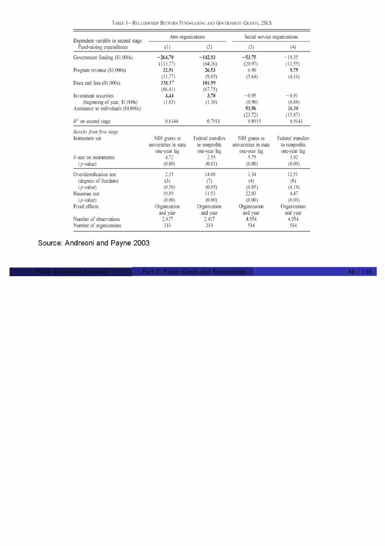
8/8/2019 Chetty - Public Economics Lectures
http://slidepdf.com/reader/full/chetty-public-economics-lectures 861/949
Early lab experiments testing free-rider behavior.
Groups of 5 subjects, each given 10 tokens.
Can invest tokens in either an individual or group account.
Individual: 1 token = $1 for me; Group: 1 token = 50 cents foreveryone
Nash equilibrium is 100% individual but Pareto e¢cient outcome is
100% group.
Compute fraction invested in group account under various treatments
Public Economics Lectures () Part 7: Public Goods and Externalities 50 / 138
8/8/2019 Chetty - Public Economics Lectures
http://slidepdf.com/reader/full/chetty-public-economics-lectures 862/949
Public Economics Lectures () Part 7: Public Goods and Externalities 51 / 138
Marwell and Ames 1981

8/8/2019 Chetty - Public Economics Lectures
http://slidepdf.com/reader/full/chetty-public-economics-lectures 863/949
Finding: 40 to 60% of tokens were still invested in the public good.
Experiment run on various groups of high school and college students.
Only one group free-rode a lot: 1st year econ graduate students (20%donation rate).
“Economists Free Ride, Does Anyone Else?”
Marglin: thinking like an economist undermines community
Public Economics Lectures () Part 7: Public Goods and Externalities 52 / 138
Andreoni 1988

8/8/2019 Chetty - Public Economics Lectures
http://slidepdf.com/reader/full/chetty-public-economics-lectures 864/949
Isaac, McCue, and Plott (1985): when the game is repeated with
same set of players, public good contribution levels fall over time.
Andreoni (1988): is this b/c of learning or strategic behavior?
Game to distinguish these two hypotheses:
10 iterations of Marwell-Ames game
Two di¤erent samples:
Group A: play with strangers
Group B: play with partners (stable groups)
Strategic hypothesis predicts strangers free ride more
Public Economics Lectures () Part 7: Public Goods and Externalities 53 / 138

8/8/2019 Chetty - Public Economics Lectures
http://slidepdf.com/reader/full/chetty-public-economics-lectures 865/949
Public Economics Lectures () Part 7: Public Goods and Externalities 54 / 138
Andreoni 1993
Uses lab experiment to directly test crowdout hypothesis with

8/8/2019 Chetty - Public Economics Lectures
http://slidepdf.com/reader/full/chetty-public-economics-lectures 866/949
p y yp“government” provision
Payo¤s U h = (7 G h)1αG α
Two groups: no-tax and tax
No-tax group can choose G h = 0, 1, 2, .., 7
Tax group automatically gets 2 tokens allocated to G and can chooseG h = 0, 1, 2, . ., 5
Each game repeated twenty times
Nash equilibrium in no-tax game is G h = 3 but Pareto e¢cientoutcome is G h = 6
Public Economics Lectures () Part 7: Public Goods and Externalities 55 / 138

8/8/2019 Chetty - Public Economics Lectures
http://slidepdf.com/reader/full/chetty-public-economics-lectures 867/949
Public Economics Lectures () Part 7: Public Goods and Externalities 56 / 138
8/8/2019 Chetty - Public Economics Lectures
http://slidepdf.com/reader/full/chetty-public-economics-lectures 868/949
Public Economics Lectures () Part 7: Public Goods and Externalities 57 / 138
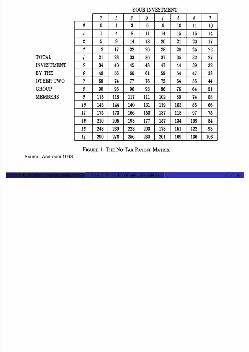
8/8/2019 Chetty - Public Economics Lectures
http://slidepdf.com/reader/full/chetty-public-economics-lectures 869/949
Public Economics Lectures () Part 7: Public Goods and Externalities 58 / 138
Andreoni 1993

8/8/2019 Chetty - Public Economics Lectures
http://slidepdf.com/reader/full/chetty-public-economics-lectures 870/949
Public good levels are signi…cantly higher in the tax case.
However, crowd-out is substantial: 71.5% on average.
Compare with empirical studies that …nd 30% crowding out.
Crowd-out increases in …nal rounds.
Considered an upper bound of degree of crowd out
Missing warm glow, social pressure, lack of salience.
Public Economics Lectures () Part 7: Public Goods and Externalities 59 / 138
Crowdout: Summary of Evidence
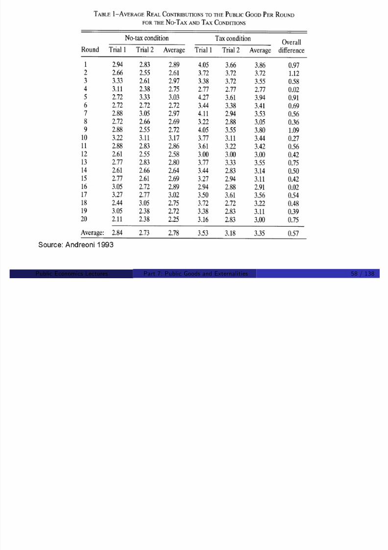
8/8/2019 Chetty - Public Economics Lectures
http://slidepdf.com/reader/full/chetty-public-economics-lectures 871/949
Rate of crowdout is probably 30 cents on the dollar on average, butprobably highly heterogeneous.
Non-trivial but far from BBV/Roberts prediction.
Key factors are probably warm glow and salience
Suggests that carefully targeted govt programs can still haveconsiderable net impact.
Public Economics Lectures () Part 7: Public Goods and Externalities 60 / 138
Financing PGs with Distortionary Taxation

8/8/2019 Chetty - Public Economics Lectures
http://slidepdf.com/reader/full/chetty-public-economics-lectures 872/949
Second problem in implementing the Samuelson Rule is that thegovernment cannot use lump sum taxation in practice because of redistributional concerns
For this section, ignore private crowdout problem
Instead, consider goods where individuals are at corners, such asroads or defense
Public Economics Lectures () Part 7: Public Goods and Externalities 61 / 138
Pigou’s Conjecture (1947)

8/8/2019 Chetty - Public Economics Lectures
http://slidepdf.com/reader/full/chetty-public-economics-lectures 873/949
Total costs of providing public good are higher than its productioncosts when it is …nanced by distortionary taxation
1 At the optimum: the MB of the public good should be equal to theMC of production plus the marginal deadweight burden of taxation
2 The optimal level of public goods with distortionary taxation is lower
relative to a 1st best where govt can use lump sum taxation
Subsequent formal analysis (Atkinson and Stern 1974) showed this is
true, but with a few caveats
Public Economics Lectures () Part 7: Public Goods and Externalities 62 / 138
PGs with Distortionary Taxes: Setup

8/8/2019 Chetty - Public Economics Lectures
http://slidepdf.com/reader/full/chetty-public-economics-lectures 874/949
Large number of identical individuals
Utility over private consumption (c ), labor (l ), and PG (G )
U (c ,
l ,
G ) = c l k +1
/(k + 1) + v (G )
Prices of c and G are both 1 (MRT = 1)
Individuals do not contribute b/c the contribution of one individual
has a negligible e¤ect on G .
Public Economics Lectures () Part 7: Public Goods and Externalities 63 / 138
PGs with Distortionary Taxes: Setup
Two policy instruments: lump sum tax R and linear tax on labor τ :

8/8/2019 Chetty - Public Economics Lectures
http://slidepdf.com/reader/full/chetty-public-economics-lectures 875/949
c = wl (1 τ ) R
Individual chooses l to maximize
wl (1 τ ) R l k +1 + v (G )
where G is viewed as …xed (individual is small).
Implies that
w (1 τ ) = l k
) l = w e (1 τ )e
where e = 1/k is the elasticity of labor supply with respect to thenet-of-tax rate 1 τ
Public good level equals tax revenue: G = wl τ + R
Public Economics Lectures () Part 7: Public Goods and Externalities 64 / 138
PGs with Distortionary Taxes: 1st Best

8/8/2019 Chetty - Public Economics Lectures
http://slidepdf.com/reader/full/chetty-public-economics-lectures 876/949
When lump sum tax instrument is available, govt maximizes
W = wl (1 τ ) R l k +1/(k + 1) + v (G )
= wl (1 τ ) R l k +1/(k + 1) + v (wl τ + R )
where l = [w (1 τ )]e
is chosen optimally by the individual
FOC in R implies that v 0(G ) = 1 (Samuelson rule)
Public good provided up to the point where sum of MRS v 0(G )/1
equal MRT 1
Public Economics Lectures () Part 7: Public Goods and Externalities 65 / 138
PGs with Distortionary Taxes: 1st Best
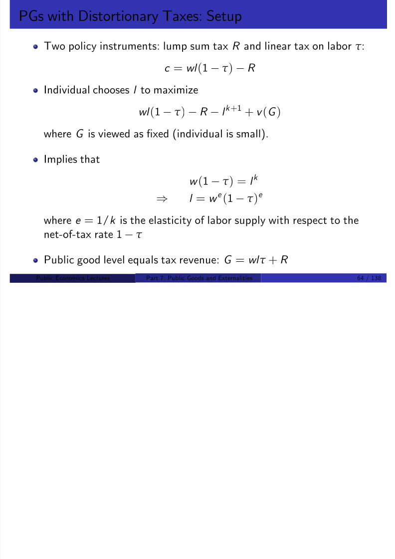
8/8/2019 Chetty - Public Economics Lectures
http://slidepdf.com/reader/full/chetty-public-economics-lectures 877/949
In …rst best, optimal linear tax is τ = 0
∂W
∂τ = wl + wlv 0(G ) + w τ v 0(G )∂l /∂τ
∂W ∂τ
= w τ v 0(G )∂l /∂τ
Therefore
∂W
∂τ (τ
) = 0 ) τ
= 0
Public Economics Lectures () Part 7: Public Goods and Externalities 66 / 138
PGs with Distortionary Taxes: 2nd Best
In second best, lump sum tax unavailable (R = 0).

8/8/2019 Chetty - Public Economics Lectures
http://slidepdf.com/reader/full/chetty-public-economics-lectures 878/949
Govt chooses τ to maximize:
W = wl (1 τ ) l k +1/(k + 1) + v (wl τ )
Using the envelope theorem yields f.o.c. for τ :
0 = ∂W /∂τ = wl + v 0(G )(wl w τ∂l /∂(1 τ ))
) 1 = v 0(G )[1 τ 1 τ
e ]
Added term τ 1τ e in formula relative to Samuelson rule
v 0(G SB ) > v 0(G FB ) = 1 which implies G SB < G FB because v (G ) isconcave
Higher threshold (MCPF > 1): depends on e .
Public Economics Lectures () Part 7: Public Goods and Externalities 67 / 138
Heterogeneity: Gaube 2000
In a setting with heterogeneity in prefs for PG (v h), proves that

8/8/2019 Chetty - Public Economics Lectures
http://slidepdf.com/reader/full/chetty-public-economics-lectures 879/949
1 Without redistributive prefs., G SB < G
FB
.
2 With redistributive tastes, could have G SB > G FB .
Intuition: if public parks bene…t mostly low income households,
over-provide parks to enhance redistribution
First-best level of redistribution cannot be achieved using standard taxinstruments.
By providing park instead of welfare, redistribute income withoutdistorting incentive to work.
Example of theory of the second best (Lipsey and Lancaster 1956)
Public Economics Lectures () Part 7: Public Goods and Externalities 68 / 138
Kreiner and Verdelin 2009
Consider a general model with non-linear income taxes (includinglump sum)
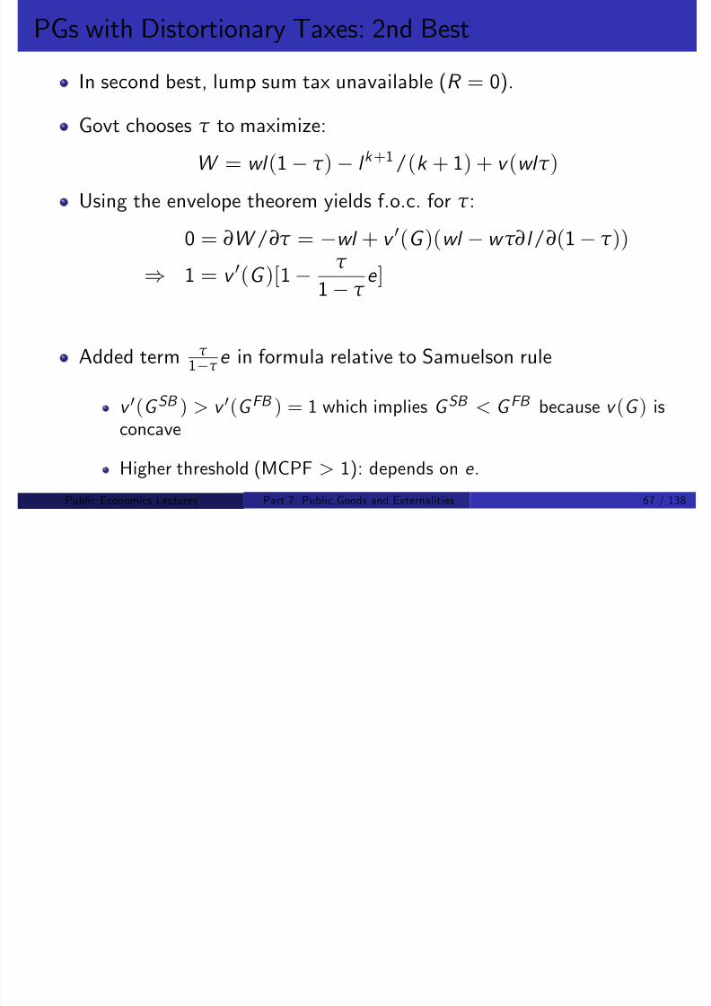
8/8/2019 Chetty - Public Economics Lectures
http://slidepdf.com/reader/full/chetty-public-economics-lectures 880/949
lump sum)
Q: What threshold should be used for PG’s in this setting?
A: Depends on whether non-linear tax system is reoptimized whenPG’s are funded
If yes, then Samuelson rule correct again
E.g. if public good bene…ts all equally, then simply raise lump sum taxand distributional problem is unchanged
More generally, changes in optimal non-linear tax system will havesecond-order e¤ects on welfare ! can be ignored.
Illustrates danger of Ramsey analyses
Public Economics Lectures () Part 7: Public Goods and Externalities 69 / 138
Subsides for Private Provision of PGs: Charitable Giving
Alternative to distortionary taxes is subsiding private provision.

8/8/2019 Chetty - Public Economics Lectures
http://slidepdf.com/reader/full/chetty-public-economics-lectures 881/949
E.g. in the U.S., charitable contributions are tax deductible ($20 biltax expenditure).
Theoretical questions:
Should we have such a subsidy?How large should such a subsidy be?What are the key determinants of the optimal subsidy?
Empirical questions:
How sensitive is charitable giving w.r.t. tax subsidies?Where does the money end up going (social value)?
Public Economics Lectures () Part 7: Public Goods and Externalities 70 / 138
Subsidies for Charity: Setup
Warm-glow model. Individual maximizes

8/8/2019 Chetty - Public Economics Lectures
http://slidepdf.com/reader/full/chetty-public-economics-lectures 882/949
U (c , g ) s.t. c + g = y τ (y θg )
where θ measures degree of deductibility of charitable insurance.
Price of giving $1 to charity is $1 θτ .
De…ne price and income elasticities:
β =1 θτ
g
∂g
∂(1 θτ )= price elasticity of charitable giving
γ =y
g ∂g
∂y = income elasticity of charitable giving
Public Economics Lectures () Part 7: Public Goods and Externalities 71 / 138
Subsidies for Charity: Setup
First consider case where govt uses tax revenue to fund same PG as
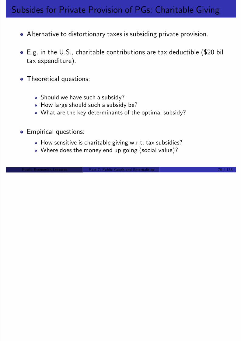
8/8/2019 Chetty - Public Economics Lectures
http://slidepdf.com/reader/full/chetty-public-economics-lectures 883/949
First consider case where govt uses tax revenue to fund same PG as
individual.
Here marginal value of PG and charity are identical.
Let P denote total funding for public good:
P = τ (y θg ) + g = k + (1 θτ )g
Question is whether to use tax subsidy and get indiv to contribute or just fund through tax revenue
Public Economics Lectures () Part 7: Public Goods and Externalities 72 / 138
Optimal Subsidies for Charity
Result 1: If β < 1 then deduction of charities unambiguouslydesirable

8/8/2019 Chetty - Public Economics Lectures
http://slidepdf.com/reader/full/chetty-public-economics-lectures 884/949
What is gained in additional contributions is larger than tax revenueloss.
P = k + (1 θτ )g
dP
d θ = τ g +
dg
d θ
1 θτ
g g
= τ g dg
d (1 θτ )
1 θτ
g τ g
= τ g βτ g
= τ g (1 + β)
Therefore β < 1 implies dP d θ > 0.
Clearly desirable to subsidize at least up to the point where β(θ) = 1.
Public Economics Lectures () Part 7: Public Goods and Externalities 73 / 138
Optimal Subsidies for Charity (Saez 2004)

8/8/2019 Chetty - Public Economics Lectures
http://slidepdf.com/reader/full/chetty-public-economics-lectures 885/949
Now consider case where marginal values of private charity and PGdi¤er
Marginal value of public spending = 1
Marginal value of private charity = λ(G )
Multiplier λ(G ) 2 [0, 1] measures external e¤ect of charitablecontributions on social welfare
Public Economics Lectures () Part 7: Public Goods and Externalities 74 / 138
Optimal Subsidies for Charity (Saez 2004)

8/8/2019 Chetty - Public Economics Lectures
http://slidepdf.com/reader/full/chetty-public-economics-lectures 886/949
With ‡at social welfare weights, optimal tax rate t G for charitablegood G satis…esλ + t G
1 + t G =
1
β
Generalizes Ramsey inverse-elasticity rule by allowing λ > 0
Analogous to Sandmo 1975 correction for externalities
If λ = 1 (PG equivalent to charity), t G should be set so that
β(t G ) = 1, as above
Public Economics Lectures () Part 7: Public Goods and Externalities 75 / 138
Optimal Subsidies for Charity (Saez 2004)

8/8/2019 Chetty - Public Economics Lectures
http://slidepdf.com/reader/full/chetty-public-economics-lectures 887/949
Key elements for optimal tax or subsidy of charitable contributions:
Who bene…ts from charitable contributions (λ)?
Are charitable contributions responsive to the subsidy ( β)?
In a many-person model with heterogeneity, need social welfare weightsof those contributing.
What are the incomes of those contributing?
P blic Economics Lect res () Part 7 P blic Goods and E ternalities 76 / 138
Empirical Evidence
Existing studies have estimated β and γ - income and price

8/8/2019 Chetty - Public Economics Lectures
http://slidepdf.com/reader/full/chetty-public-economics-lectures 888/949
g β γ p
elasticities.
General speci…cation:
log(g ) = α + β log(1 τ ) + γ log y +
Early work (Feldstein and Taylor 1976, Clotfelter 1985):cross-sectional regressions with controls.
Results: γ = 0.8, β = 1.3.
But results confounded: e¤ectively comparing rich and poor
P bli E i L t () P t 7 P bli G d d E t liti 77 / 138
Empirical Evidence: Randolph (1995)

8/8/2019 Chetty - Public Economics Lectures
http://slidepdf.com/reader/full/chetty-public-economics-lectures 889/949
Uses ten year tax return panel (1979-1988) and …ts DD-type models.
Finds short-term elasticities: 1.2; long-term elasticities: 0.6.
Income e¤ects are larger in the long-term than in the short-term.
P bli E i L t () P t 7 P bli G d d E t liti 78 / 138
Externalities: Outline

8/8/2019 Chetty - Public Economics Lectures
http://slidepdf.com/reader/full/chetty-public-economics-lectures 890/949
1 De…nition and Basic Model
2 Correcting Externalities
3
Prices vs. Quantities (Weitzman 1974)
4 2nd Best Taxation with Externalities (Sandmo 1975)
5 Empirical Applications
P bli E i L t () P t 7 P bli G d d E t liti 79 / 138
De…nition
An externality arises whenever the utility or production possibility of t d d di tl th ti f th t

8/8/2019 Chetty - Public Economics Lectures
http://slidepdf.com/reader/full/chetty-public-economics-lectures 891/949
an agent depends directly on the actions of another agent.
Important distinction between “pecuniary” vs. “non-pecuniary”externalities
Consuming an apple vs. consuming loud music
Not a technological distinction; depends on market in place
Coasian view: can convert all externalities into pecuniary externalities
with appropriate markets, property rights.
Only non-pecuniary externalities justify policy intervention
P bli E i L t () P t 7 P bli G d d E t liti 80 / 138
Externalities: Main Questions

8/8/2019 Chetty - Public Economics Lectures
http://slidepdf.com/reader/full/chetty-public-economics-lectures 892/949
1 Theoretical: what is the best way to correct externalities and movecloser to the social optimum?
2 Empirical: how to measure the size of externalities?
Key di¤erence: cannot use standard revealed-preference methods
Public Economics Lectures () Part 7: Public Goods and Externalities 81 / 138
Model of Externalities
Firms produce x cars using c (x ) units of the numeraire y .

8/8/2019 Chetty - Public Economics Lectures
http://slidepdf.com/reader/full/chetty-public-economics-lectures 893/949
Generates x units of pollution: P (x ) = x .
Consumers have wealth Z and quasilinear utility:
u (x ) + y d P (x )
where d = marginal damage (MD) of pollution
Social welfare is
W = u (x ) + Z c (x ) d x
Let p denote the market price of cars.
Public Economics Lectures () Part 7: Public Goods and Externalities 82 / 138
Model of Externalities: Equilibrium
Firms max pro…ts:max px c (x )
8/8/2019 Chetty - Public Economics Lectures
http://slidepdf.com/reader/full/chetty-public-economics-lectures 894/949
Consumers max utility, taking level of pollution as …xed:
max u (x ) + Z px
Demand satis…es
u 0(x D ) = p
Supply satis…esc 0(x S ) = p
PMB equals PMC in equilibrium:
u 0(x D ) = c 0(x S )
But this is not Pareto e¢cient
Public Economics Lectures () Part 7: Public Goods and Externalities 83 / 138
SMC =PMC +MD Price
Negative Production Externalities: Pollution
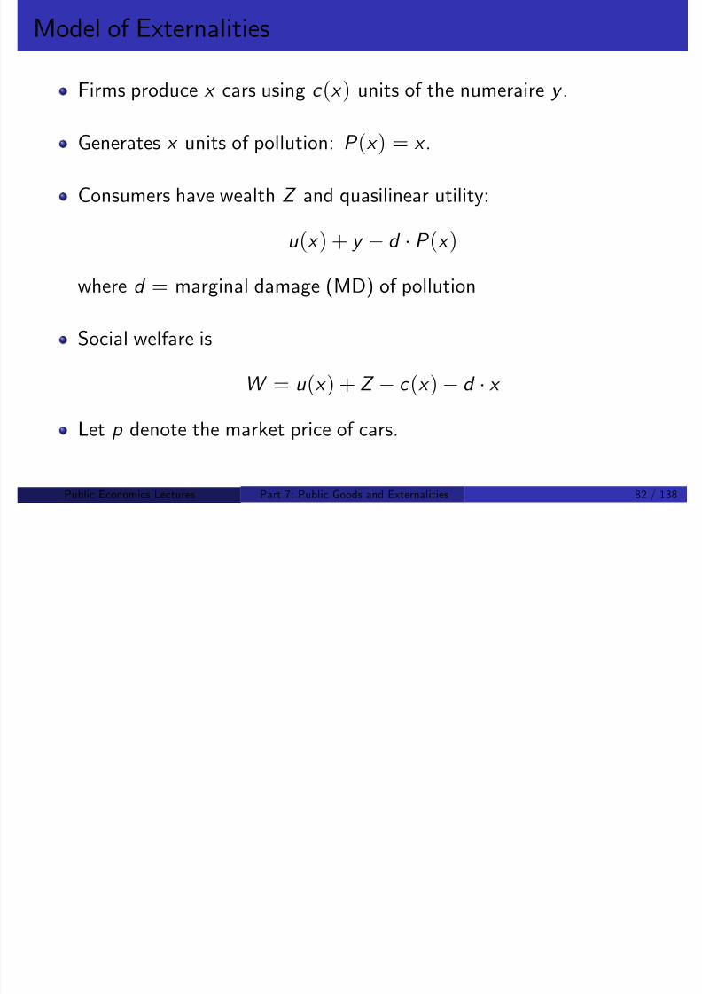
8/8/2019 Chetty - Public Economics Lectures
http://slidepdf.com/reader/full/chetty-public-economics-lectures 895/949
Quantity0 Q*
D = PMB = SMB
QM
P*
S=PMC
MD
PM
Public Economics Lectures () Part 7: Public Goods and Externalities 84 / 138
Model of Externalities: Deadweight Loss

8/8/2019 Chetty - Public Economics Lectures
http://slidepdf.com/reader/full/chetty-public-economics-lectures 896/949
Perturbation argument: can increase social welfare by reducingproduction by ∆x :
dW = u 0(x )∆x c 0(x )∆x d ∆x
= d ∆x >
0 if ∆x <
0
First Welfare Theorem does not hold
Analogous result for consumption externalities
Public Economics Lectures () Part 7: Public Goods and Externalities 85 / 138
Price
Negative Consumption Externalities
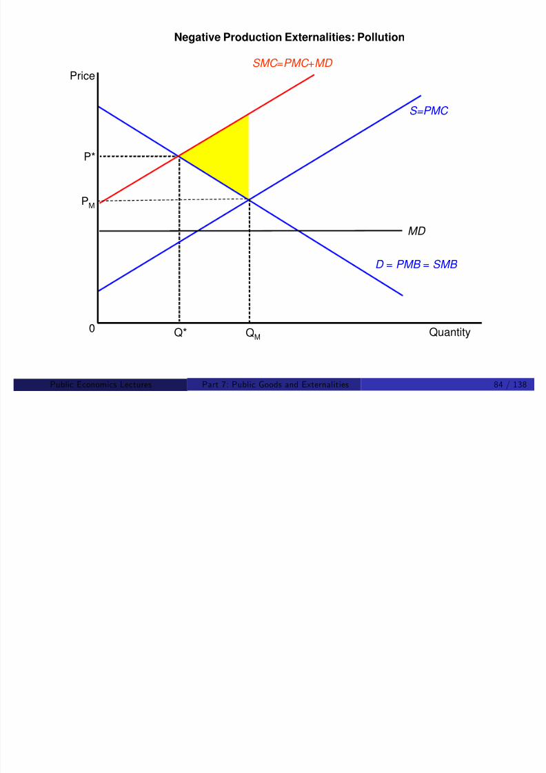
8/8/2019 Chetty - Public Economics Lectures
http://slidepdf.com/reader/full/chetty-public-economics-lectures 897/949
Quantity0 Q*
D = PMB
QM
PM
S=PMC=SMC
P*MD
SMB =PMB -MD
Public Economics Lectures () Part 7: Public Goods and Externalities 86 / 138
Remedies for Externalities
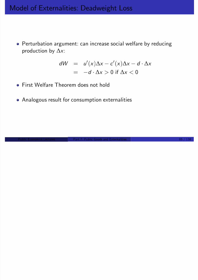
8/8/2019 Chetty - Public Economics Lectures
http://slidepdf.com/reader/full/chetty-public-economics-lectures 898/949
1 Coasian bargaining solution
2 Pigouvian corrective taxation
3 Regulation
4 Permits (cap-and-trade)
Public Economics Lectures () Part 7: Public Goods and Externalities 87 / 138
Coasian Solution
Externalities emerge because property rights are not well de…ned.

8/8/2019 Chetty - Public Economics Lectures
http://slidepdf.com/reader/full/chetty-public-economics-lectures 899/949
Establish property rights to create markets for pollution.
Consider example of pollution in a river.
If consumer owns river, in competitive equilibrium, …rms pay d forevery unit of pollution emitted.
Marginal cost of production is now c 0(x ) + d , leading to 1st best.
Symmetric solution when …rm owns river.
Assignment of property rights a¤ects distribution but not e¢ciency
Public Economics Lectures () Part 7: Public Goods and Externalities 88 / 138
Coasian Solution: Limitations
1 Cost of bargaining
8/8/2019 Chetty - Public Economics Lectures
http://slidepdf.com/reader/full/chetty-public-economics-lectures 900/949
Ex: air pollution – would require millions of agents to coordinate andbargain
To reduce transactions costs, need an association to represent agents
This “association” is the government
2 Asymmetric information: competitive equilibrium can break down
Often hard to identify precise source of damage
E.g. atmospheric pollution very di¤use, marginal damages unclear
Public Economics Lectures () Part 7: Public Goods and Externalities 89 / 138
Pigouvian Taxation

8/8/2019 Chetty - Public Economics Lectures
http://slidepdf.com/reader/full/chetty-public-economics-lectures 901/949
Impose tax t = MD (Q )
Restores Pareto e¢ciency and maximizes social welfare
Practical limitations:
Must know marginal damage function to set t
Di¢cult to measure the marginal damage in practice
Public Economics Lectures () Part 7: Public Goods and Externalities 90 / 138
Pigouvian Tax
S PMC
SMC =PMC +MD S =PMC +tPrice

8/8/2019 Chetty - Public Economics Lectures
http://slidepdf.com/reader/full/chetty-public-economics-lectures 902/949
Quantity0 Q*
D = PMB = SMB
Q1
P1
S=PMC
P*
P2
Q2
$t
Public Economics Lectures () Part 7: Public Goods and Externalities 91 / 138
Regulation: Command and Control
Must reduce pollution to set level or face legal sanctions.

8/8/2019 Chetty - Public Economics Lectures
http://slidepdf.com/reader/full/chetty-public-economics-lectures 903/949
Same outcome as Pigouvian taxation: move people to x 2
Advantages:
1 Ease of enforcement
2 Salience, political
expedience
Disadvantages:
1 Dynamics: no incentive toinnovate
2 Allocative ine¢ciency
with heterogeneity in costof pollution reduction
Public Economics Lectures () Part 7: Public Goods and Externalities 92 / 138
Permits: Cap-and-Trade
Cap total amount of pollution and allow …rms to trade permits topollute

8/8/2019 Chetty - Public Economics Lectures
http://slidepdf.com/reader/full/chetty-public-economics-lectures 904/949
Address disadvantages of regulation using an auction-based permitsystem.
Hybrid of regulation and Coasian solution.
In eq., …rms with highest MC of reducing pollution will buy permits;those that can easily reduce pollution will do so.
If total number of permits is set to achieve the social optimum, both
allocative and productive e¢ciency will be achieved.
Also have dynamic incentives to innovate because each …rm is bearinga marginal cost of pollution.
Public Economics Lectures () Part 7: Public Goods and Externalities 93 / 138
Weitzman 1974: Prices vs. Quantities

8/8/2019 Chetty - Public Economics Lectures
http://slidepdf.com/reader/full/chetty-public-economics-lectures 905/949
Price mechanism (taxes) identical to quantity mechanism (permits) insimple model above. How to choose?
Weitzman (1974): with uncertainty re. shape of MB and MC curves,
price and quantity no longer equivalent.
Now the standard method of choosing between regulation and taxes
Public Economics Lectures () Part 7: Public Goods and Externalities 94 / 138
Weitzman 1974: Market for Pollution Reduction
Let q denote pollution reduction starting from private market eq.,where q = 0.

8/8/2019 Chetty - Public Economics Lectures
http://slidepdf.com/reader/full/chetty-public-economics-lectures 906/949
Let B (Q ) denote social bene…ts of pollution reduction
Let C (Q ) denote social costs.
In simple model above:
MB of pollution reduction is constant, B 0(Q ) = d .
MC given by loss in surplus from producing one less car: u 0
(x
)c 0
(x
).
More generally, MC should be interpreted as cost of reducing pollutionthrough cheapest method (e.g. cleaner plants)
Public Economics Lectures () Part 7: Public Goods and Externalities 95 / 138
Market for Pollution Reduction
PMC Q =SMC
Q
Price

8/8/2019 Chetty - Public Economics Lectures
http://slidepdf.com/reader/full/chetty-public-economics-lectures 907/949
SMB Q
Q* Pollution Reduction
Public Economics Lectures () Part 7: Public Goods and Externalities 96 / 138
Weitzman Model: Policy without Uncertainty
In eq’m, PMB of pollution reduction is 0 ) level of pollutionreduction is Q = 0.

8/8/2019 Chetty - Public Economics Lectures
http://slidepdf.com/reader/full/chetty-public-economics-lectures 908/949
Social optimum:maxB (Q ) C (Q )
First order condition:
C
0
(Q
) = B
0
(Q
)With no uncertainty, can obtain optimum with either quantity or pricepolicy.
Quantity: require amount Q .
Price: set price for pollution reduction of p = C 0(Q ).
Public Economics Lectures () Part 7: Public Goods and Externalities 97 / 138
Weitzman: Optimal Policy with Uncertainty
Now suppose that there is uncertainty about the marginal costs of reducing pollution.

8/8/2019 Chetty - Public Economics Lectures
http://slidepdf.com/reader/full/chetty-public-economics-lectures 909/949
Cost is now C (Q , θ) with θ unknown.
Marginal cost lies between MC LB and MC UB , with mean value givenby MC mean .
Objective: maximize expected social welfare
Formally, choose one of two options: p or Q directly:
maxfE θB (Q ) C (Q , θ), E θB (Q (p )) C (Q (p ), θ)g
Choice depends on steepness of marginal bene…t curve.
Public Economics Lectures () Part 7: Public Goods and Externalities 98 / 138
MB steep, Quantity regulation

8/8/2019 Chetty - Public Economics Lectures
http://slidepdf.com/reader/full/chetty-public-economics-lectures 910/949
Public Economics Lectures () Part 7: Public Goods and Externalities 99 / 138
MB Steep, Price Regulation

8/8/2019 Chetty - Public Economics Lectures
http://slidepdf.com/reader/full/chetty-public-economics-lectures 911/949
Public Economics Lectures () Part 7: Public Goods and Externalities 100 / 138
Quantity Regulation Price Regulation

8/8/2019 Chetty - Public Economics Lectures
http://slidepdf.com/reader/full/chetty-public-economics-lectures 912/949
Public Economics Lectures () Part 7: Public Goods and Externalities 101 / 138
Price Band vs. Quantity Band with Steep MB
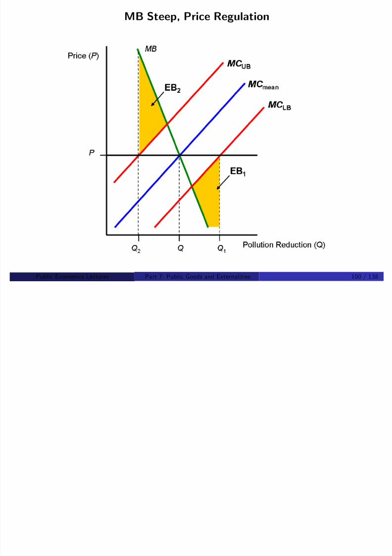
8/8/2019 Chetty - Public Economics Lectures
http://slidepdf.com/reader/full/chetty-public-economics-lectures 913/949
Public Economics Lectures () Part 7: Public Goods and Externalities 102 / 138
MB Flat, Quantity Regulation

8/8/2019 Chetty - Public Economics Lectures
http://slidepdf.com/reader/full/chetty-public-economics-lectures 914/949
Public Economics Lectures () Part 7: Public Goods and Externalities 103 / 138
MB Flat, Price Regulation

8/8/2019 Chetty - Public Economics Lectures
http://slidepdf.com/reader/full/chetty-public-economics-lectures 915/949
Public Economics Lectures () Part 7: Public Goods and Externalities 104 / 138
Quantity regulation Price Regulation

8/8/2019 Chetty - Public Economics Lectures
http://slidepdf.com/reader/full/chetty-public-economics-lectures 916/949
Public Economics Lectures () Part 7: Public Goods and Externalities 105 / 138
Weitzman: Uncertainty about Bene…ts
Now suppose that there is uncertainty about the marginal bene…ts of reducing pollution but that the costs are known.
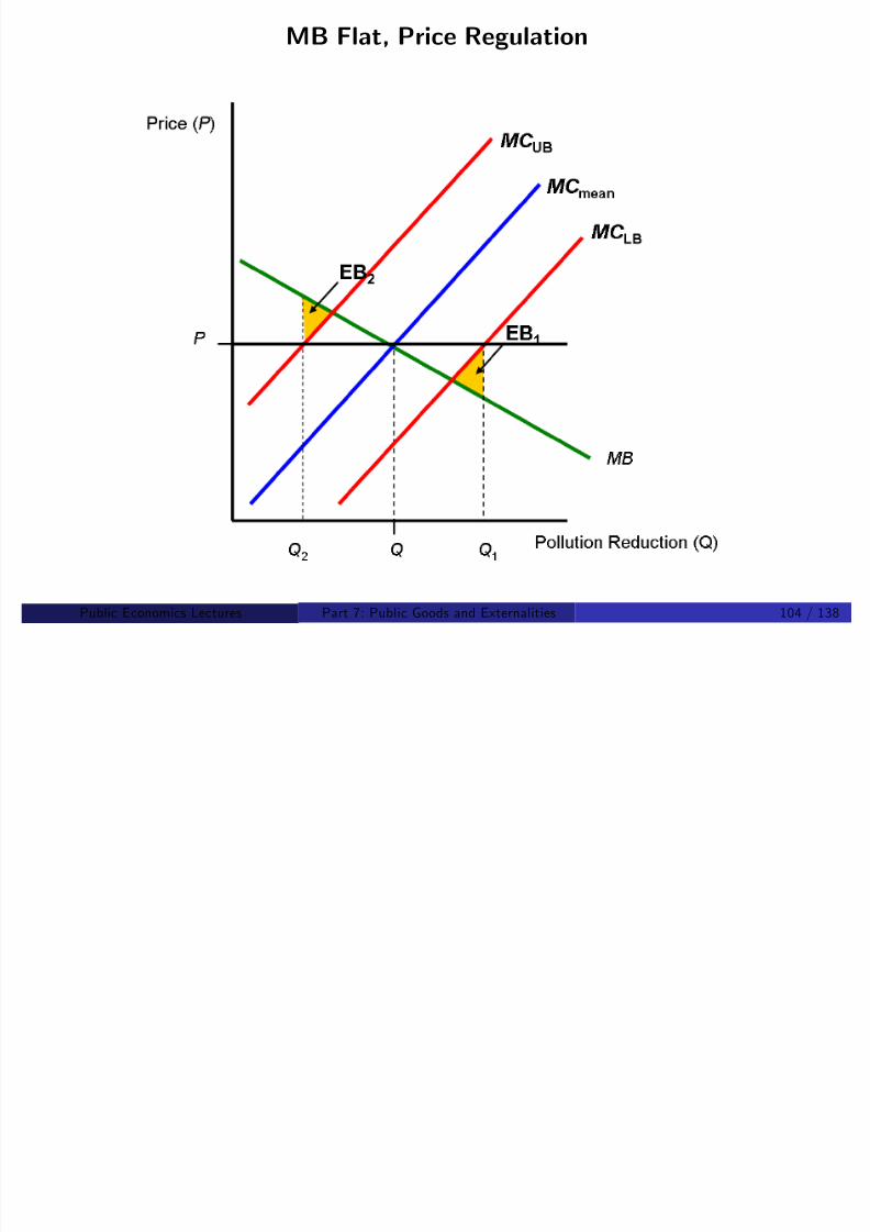
8/8/2019 Chetty - Public Economics Lectures
http://slidepdf.com/reader/full/chetty-public-economics-lectures 917/949
Price and quantity policies are again equivalent.
For a given p , the government knows the Q that will result exactlysince p = C 0(Q ).
More generally, uncertainty matters only when it is about thecost/bene…t schedule for the agent who chooses level of pollutionreduction.
If consumer chooses level of pollution reduction, then only uncertaintyabout marginal bene…ts matters
Public Economics Lectures () Part 7: Public Goods and Externalities 106 / 138
Optimal Second-Best Taxation with Externalities
In general, cannot restore 1st best b/c externality is one of manyd i i f … b

8/8/2019 Chetty - Public Economics Lectures
http://slidepdf.com/reader/full/chetty-public-economics-lectures 918/949
deviations from …rst best.
Most important other deviation: govt also uses distortionary taxes to…nance public goods and redistribute income.
Sandmo (1975): optimal tax policy with externalities and a revenuerequirement.
Combination of Ramsey and Pigou problems
Public Economics Lectures () Part 7: Public Goods and Externalities 107 / 138
Sandmo 1975: Setup
Denote by d (x N ) the externality cost of consumption of good N
Let w be the age rate and qi pi + τi denote post ta prices
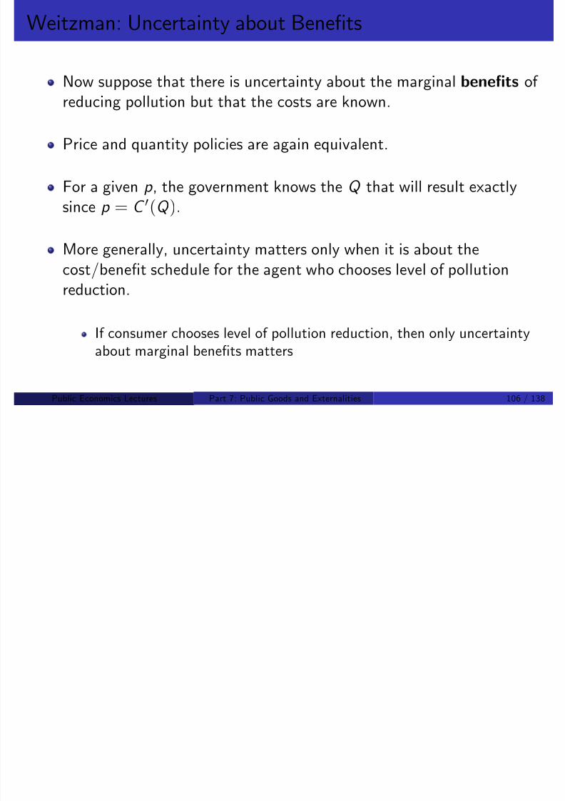
8/8/2019 Chetty - Public Economics Lectures
http://slidepdf.com/reader/full/chetty-public-economics-lectures 919/949
Let w be the wage rate and q i = p i + τ i denote post-tax prices.
Let Z denote non wage income.
Producer prices …xed; all pre tax prices normalized to 1.
Individuals have utility functions of the following form:
u (x 1 , . ., x N , l ) d (x N )
Utility is maximized subject to:
q 1x 1 + .. + q N x N wl + Z
Public Economics Lectures () Part 7: Public Goods and Externalities 108 / 138
Sandmo 1975: Setup
Individual maximization program
L = u (x 1 , .., x N , l ) + λ(wl + Z (q 1x 1 + .. + q N x N ))

8/8/2019 Chetty - Public Economics Lectures
http://slidepdf.com/reader/full/chetty-public-economics-lectures 920/949
Maximization yields indirect utility v (q ).
Government maximization program:
maxq
W (q ) = v (q ) d (q )
s.t. ∑ τ i x i R
Analogous to Ramsey tax problem, but here SWF di¤ers from privatesector objective
Public Economics Lectures () Part 7: Public Goods and Externalities 109 / 138
Sandmo 1975
Let θ = marginal social welfare gain from $1 of a lump sum tax and
λ marginal value of relaxing agent’s budget constraint

8/8/2019 Chetty - Public Economics Lectures
http://slidepdf.com/reader/full/chetty-public-economics-lectures 921/949
λ = marginal value of relaxing agent s budget constraint
τ ip = optimal Pigouvian tax rate (when R = 0)
τ ip = 0 for goods 1 to N 1 and τ ip = d 0
(x N ) for good N
τ ir = optimal Ramsey tax rate (when d (x n) = 0)
Let τ i denote optimal tax rate in Sandmo model
Public Economics Lectures () Part 7: Public Goods and Externalities 110 / 138
Sandmo 1975: Additivity Result
Main result: can express optimal tax rate as Ramsey rate plusPigouvian correction.
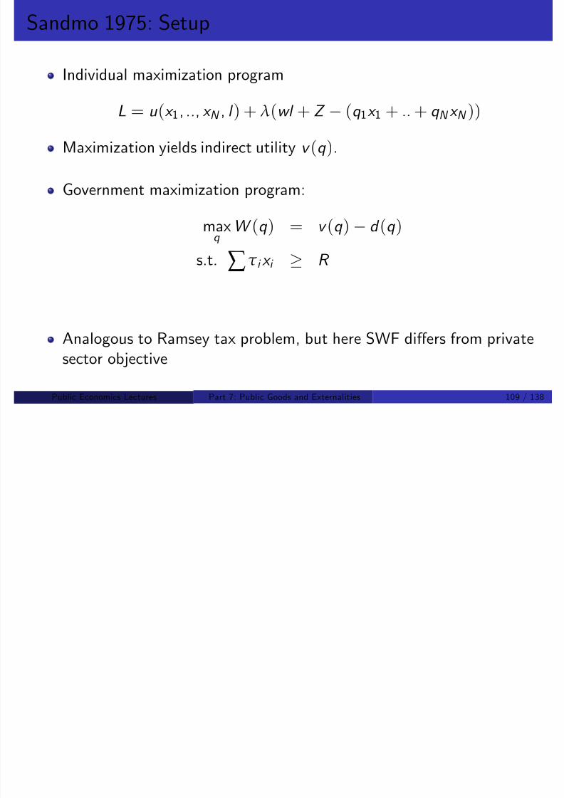
8/8/2019 Chetty - Public Economics Lectures
http://slidepdf.com/reader/full/chetty-public-economics-lectures 922/949
Consider case where Slutsky matrix is diagonal (zero cross-priceelasticities)
Then optimal tax on good i , τ i satis…esτ i τ ip 1 + τ i
= (θ/λ)/c ii
) τ i =θx c i
λ
/dx c i
dp i
+ τ ip
= τ ip + τ ir
Public Economics Lectures () Part 7: Public Goods and Externalities 111 / 138
Sandmo 1975: Additivity Result
Useful analytic representation but not an explicit formula for theoptimal tax rate
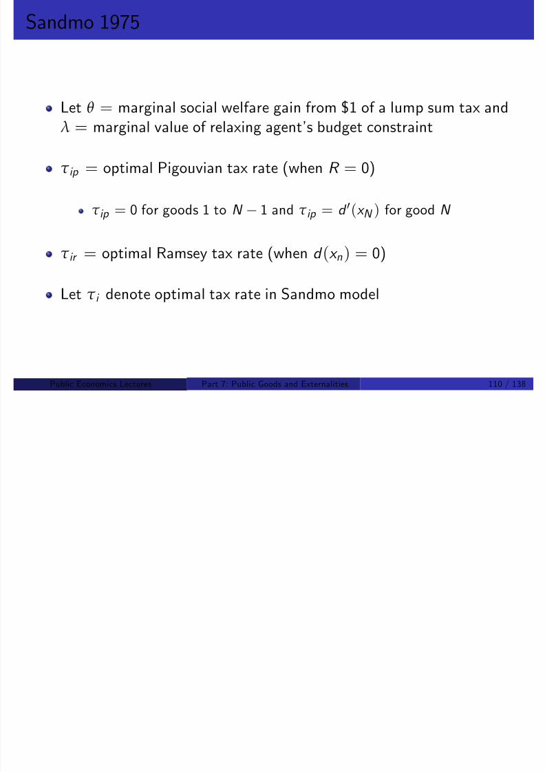
8/8/2019 Chetty - Public Economics Lectures
http://slidepdf.com/reader/full/chetty-public-economics-lectures 923/949
Ramsey tax will a¤ect level of cons, which a¤ects optimal Pigouvian taxConversely, Pigouvian tax will a¤ect optimal Ramsey tax rate
Qualitative lesson: no justi…cation to tax goods that are
complementary to those that produce negative externalities.
Just tax fuel, not cars
Optimal policy is always to directly tax source of the externality
Cornaglia and Adda (2003) example of tax on number of cigarettes vs.cotinine levels
Public Economics Lectures () Part 7: Public Goods and Externalities 112 / 138
Double Dividend Debate
Claim: gas tax has two “dividends”
1 discourages pollution raising social welfare
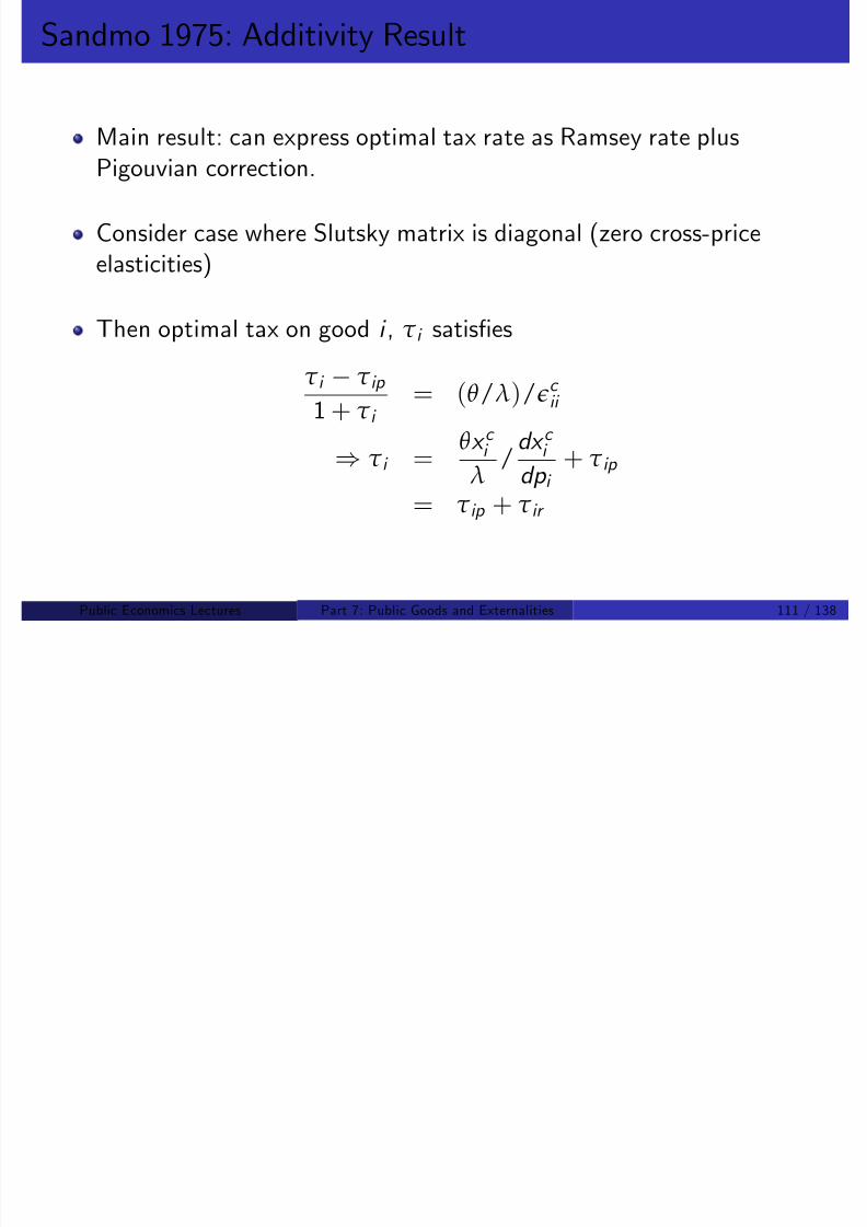
8/8/2019 Chetty - Public Economics Lectures
http://slidepdf.com/reader/full/chetty-public-economics-lectures 924/949
discourages pollution, raising social welfare2 allows govt. to reduce other distortionary taxes, improving e¢ciency.
True if we are at a corner where revenue req. is below level what is
generated by optimal Pigouvian taxes.
More realistic case: already at a Ramsey-tax interior optimum.
Suppose we discover that production of computers generates negative
externality
Public Economics Lectures () Part 7: Public Goods and Externalities 113 / 138
Double Dividend Debate
Is there a double dividend from taxing computers?
No. Already at Ramsey optimum ! no e¢ciency gain from raisingtaxes on PC’s and reducing taxes on other goods

8/8/2019 Chetty - Public Economics Lectures
http://slidepdf.com/reader/full/chetty-public-economics-lectures 925/949
taxes on PC s and reducing taxes on other goods
Only get single dividend of improving environment
Obtain double dividend only if taxes on polluting good were initiallytoo low from a Ramsey perspective.
General lesson: separate externality and optimal second-best taxproblems.
Measure externalities and identify optimal corrective taxes withoutworrying about other aspects of tax system.
Public Economics Lectures () Part 7: Public Goods and Externalities 114 / 138
Externalities: Empirical Measurement

8/8/2019 Chetty - Public Economics Lectures
http://slidepdf.com/reader/full/chetty-public-economics-lectures 926/949
Two approaches
Indirect market-based methods
Contingent valuation
Public Economics Lectures () Part 7: Public Goods and Externalities 115 / 138
Edlin and Karaca-Mandic 2006Accident externalities from driving automobiles.
If I drive, I increase probability you will get into an accident !
externality cost imposed on you

8/8/2019 Chetty - Public Economics Lectures
http://slidepdf.com/reader/full/chetty-public-economics-lectures 927/949
externality cost imposed on you
How to estimate this externality cost and appropriate Pigouvian taxon driving?
Examine relationship between tra¢c density and per-capita insurancecosts and premiums.
Look at slope to infer size of externality cost.
Identi…cation assumption: variation in tra¢c density at state level notcorrelated with other determinants of premiums (e.g. types of cars,etc.).
Public Economics Lectures () Part 7: Public Goods and Externalities 116 / 138

8/8/2019 Chetty - Public Economics Lectures
http://slidepdf.com/reader/full/chetty-public-economics-lectures 928/949
Public Economics Lectures () Part 7: Public Goods and Externalities 117 / 138
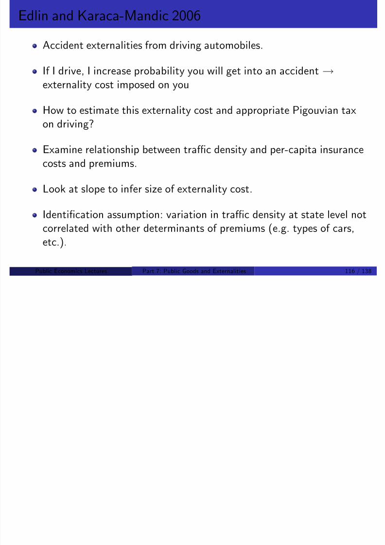
8/8/2019 Chetty - Public Economics Lectures
http://slidepdf.com/reader/full/chetty-public-economics-lectures 929/949
Public Economics Lectures () Part 7: Public Goods and Externalities 118 / 138
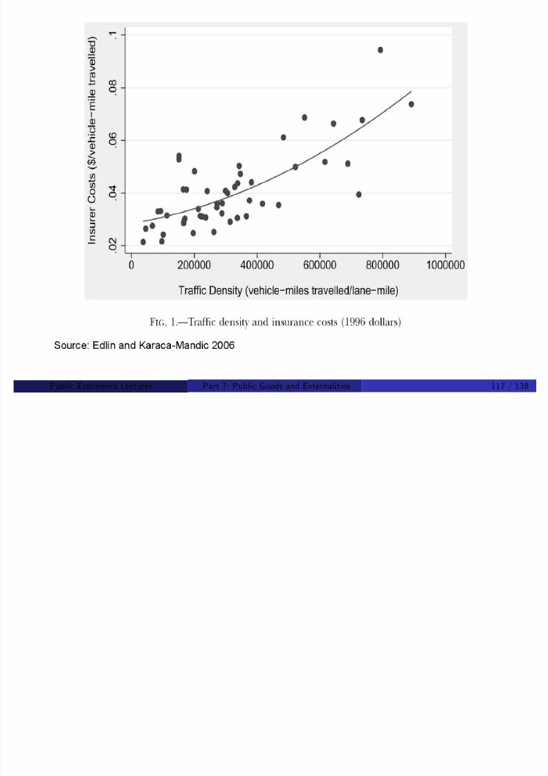
8/8/2019 Chetty - Public Economics Lectures
http://slidepdf.com/reader/full/chetty-public-economics-lectures 930/949
Public Economics Lectures () Part 7: Public Goods and Externalities 119 / 138
Edlin and Karaca-Mandic 2006
Conclude that tra¢c density substantially increases insurer costs, andthat relationship is convex

8/8/2019 Chetty - Public Economics Lectures
http://slidepdf.com/reader/full/chetty-public-economics-lectures 931/949
p
Increase in tra¢c density from average driver has external cost of $2,000 per year in California
Comparable …gure in $10 per year in North Dakota
Suggests that insurance premiums should be doubled in CA to achievesocial optimum
Public Economics Lectures () Part 7: Public Goods and Externalities 120 / 138
Brookshire et al. 1982
Infer willingness to pay for clean air using e¤ect of pollution onproperty prices (capitalization)
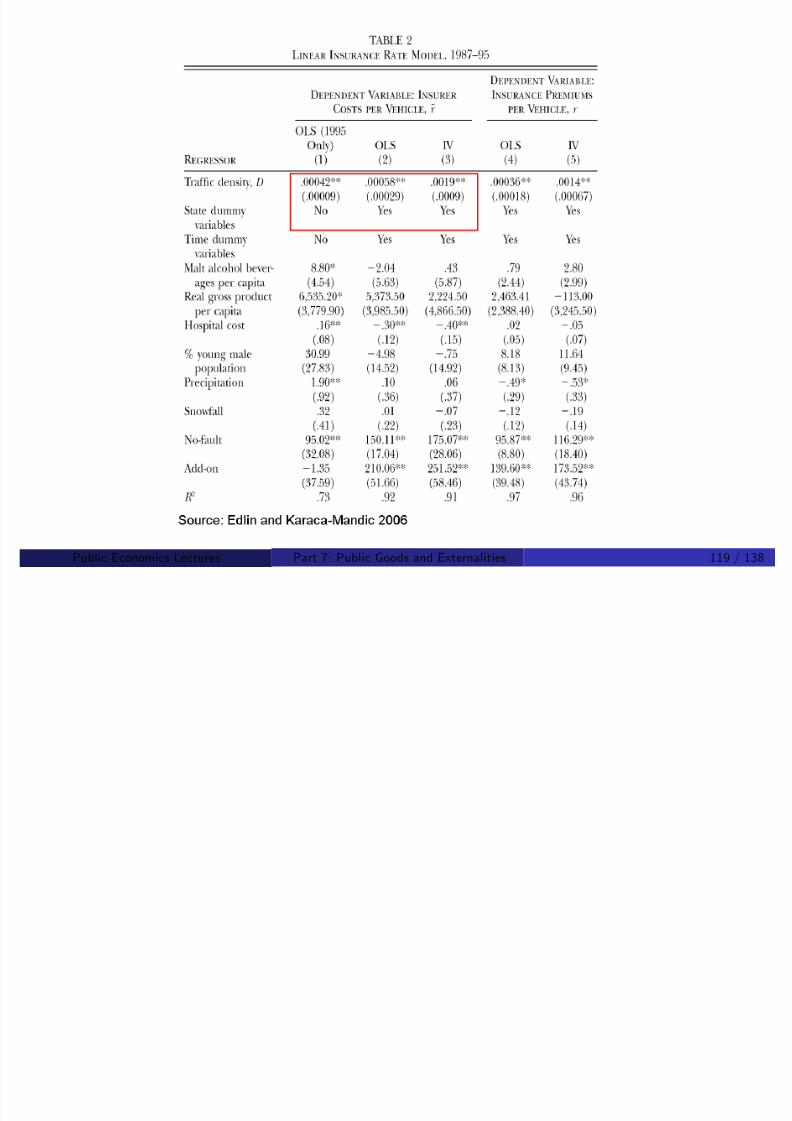
8/8/2019 Chetty - Public Economics Lectures
http://slidepdf.com/reader/full/chetty-public-economics-lectures 932/949
Compare prices of houses in polluted vs non-polluted areas.
P i = α + Pollutioni + X i β + i
Problems
Omitted variable bias: polluted neighborhoods worse on manydimensions
Sorting: people with allergies avoid polluted areas
Public Economics Lectures () Part 7: Public Goods and Externalities 121 / 138
Chay and Greenstone 2005
Also study home prices but use Clean Air Act as an exogenous change
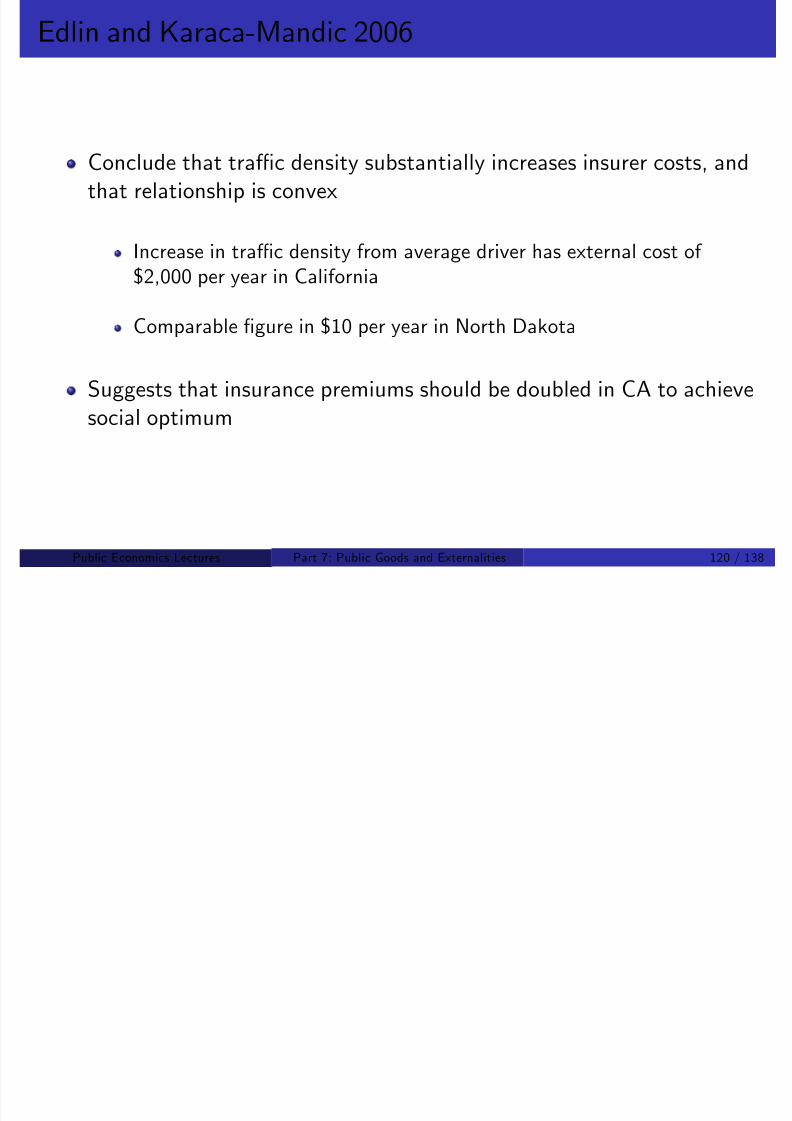
8/8/2019 Chetty - Public Economics Lectures
http://slidepdf.com/reader/full/chetty-public-economics-lectures 933/949
in pollution.
Clean Air Act: imposed ceilings on pollution levels by county in mid1970s.
High pollution counties experience sharp reductions in pollution levelsrelative to low pollution counties
Public Economics Lectures () Part 7: Public Goods and Externalities 122 / 138

8/8/2019 Chetty - Public Economics Lectures
http://slidepdf.com/reader/full/chetty-public-economics-lectures 934/949
Public Economics Lectures () Part 7: Public Goods and Externalities 123 / 138

8/8/2019 Chetty - Public Economics Lectures
http://slidepdf.com/reader/full/chetty-public-economics-lectures 935/949
Public Economics Lectures () Part 7: Public Goods and Externalities 124 / 138
Chay and Greenstone 2005
Conclusion: 1% increase in pollution ! 0.25% decline in house values

8/8/2019 Chetty - Public Economics Lectures
http://slidepdf.com/reader/full/chetty-public-economics-lectures 936/949
Clean air act increased house values by $45 bil (5%) in treatedcounties
Conceptual concern with short-run market-based methods: peoplemay not be fully aware of changes in pollution
Public Economics Lectures () Part 7: Public Goods and Externalities 125 / 138
Glaeser and Luttmer 2003
Quantify e¢ciency costs of pure command-and-control solutionsinstead of price/tradeable permit mechanisms
St d ll ti f t t d t t l

8/8/2019 Chetty - Public Economics Lectures
http://slidepdf.com/reader/full/chetty-public-economics-lectures 937/949
Study allocation of apartments under rent control
Traditionally assume that with price controls, still have allocativee¢ciency.
But regulation will generally lead to allocative ine¢ciency thatgenerates …rst-order welfare losses.
For small price caps, allocation ine¢ciency dwarfs undersupplyine¢ciency.
Public Economics Lectures () Part 7: Public Goods and Externalities 126 / 138
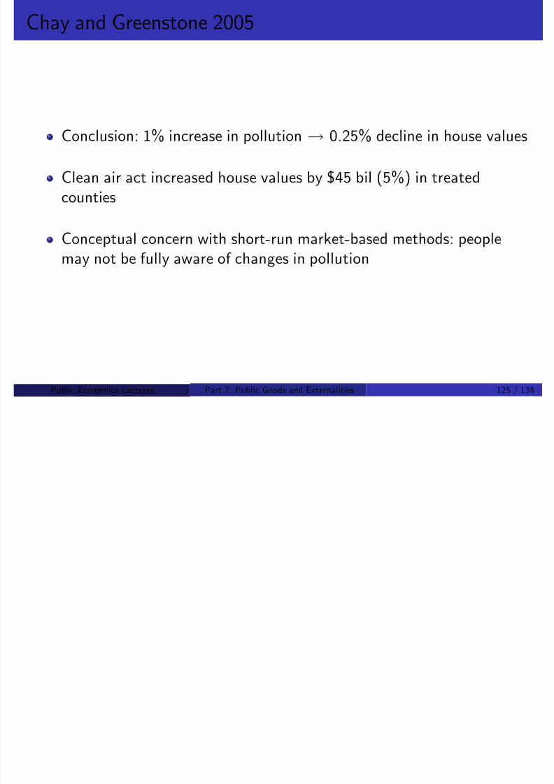
8/8/2019 Chetty - Public Economics Lectures
http://slidepdf.com/reader/full/chetty-public-economics-lectures 938/949
Public Economics Lectures () Part 7: Public Goods and Externalities 127 / 138

8/8/2019 Chetty - Public Economics Lectures
http://slidepdf.com/reader/full/chetty-public-economics-lectures 939/949
Public Economics Lectures () Part 7: Public Goods and Externalities 128 / 138

8/8/2019 Chetty - Public Economics Lectures
http://slidepdf.com/reader/full/chetty-public-economics-lectures 940/949
Public Economics Lectures () Part 7: Public Goods and Externalities 129 / 138
Glaeser and Luttmer 2003
Quantify welfare losses from misallocation by comparing consumptionpatterns in rent-controlled (NYC) and free-market places across
demographic groups.
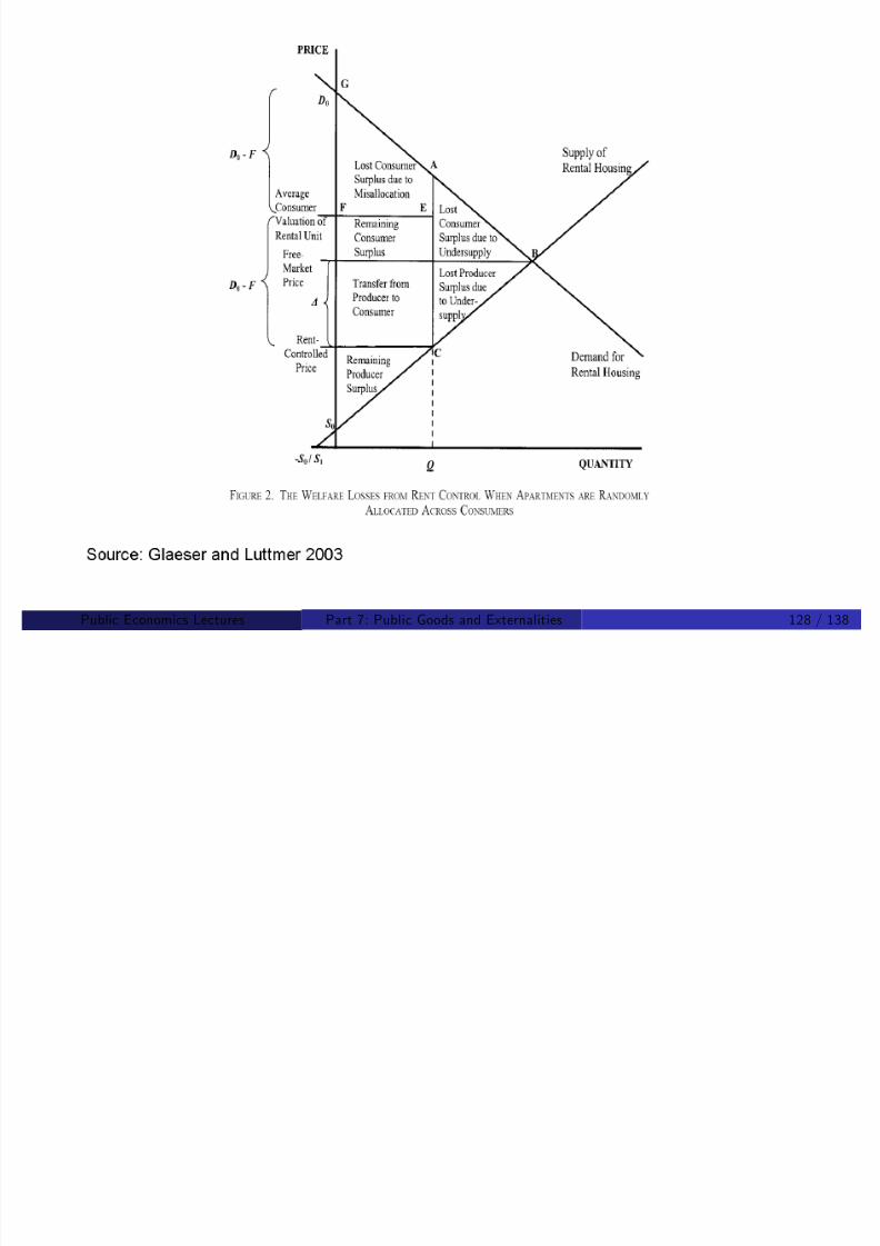
8/8/2019 Chetty - Public Economics Lectures
http://slidepdf.com/reader/full/chetty-public-economics-lectures 941/949
Predict apartment size using number in family, income, education,age, etc. using 105 large MSAs
Test if actual apartment allocations in NYC match predictions
Identifying assumption: preferences stable across MSAs
Check: placebo tests using Chicago and Hartford
Public Economics Lectures () Part 7: Public Goods and Externalities 130 / 138

8/8/2019 Chetty - Public Economics Lectures
http://slidepdf.com/reader/full/chetty-public-economics-lectures 942/949
Public Economics Lectures () Part 7: Public Goods and Externalities 131 / 138
Contingent Valuation
For some outcomes, it is impossible to have a market value

8/8/2019 Chetty - Public Economics Lectures
http://slidepdf.com/reader/full/chetty-public-economics-lectures 943/949
Ex: protecting endangered species
Common solution: “contingent valuation” surveys
How much would you be willing to pay to avoid extinction of whales?
Public Economics Lectures () Part 7: Public Goods and Externalities 132 / 138
Diamond and Hausman 1994
Describe problems with contingent valuation using surveys
No resource cost to respondents
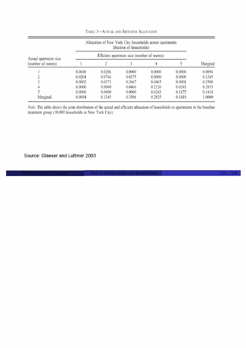
8/8/2019 Chetty - Public Economics Lectures
http://slidepdf.com/reader/full/chetty-public-economics-lectures 944/949
Lack of consistency in responses
Framing E¤ects: whales then seals vs. seals then whalesWTP to clean one lake = WTP to clean 5 lakes
Diamond and Hausman: let experts decide based on a budget voted
on by individuals for the environment instead of relying on valuation
Public Economics Lectures () Part 7: Public Goods and Externalities 133 / 138
Behavioral Economics Applications: Internalities
Sin taxes intended to correct “internalities.”
Internal costs of smoking cigarettes dwarf the external costs.

8/8/2019 Chetty - Public Economics Lectures
http://slidepdf.com/reader/full/chetty-public-economics-lectures 945/949
Suggests that conventional Pigouvian taxation should be small(relative to actual taxes observed on e.g. cigarettes and alcohol).
Q: Does addictive nature of cigarettes motivate taxation?
A: Highly sensitive to positive model of addiction
Challenge: di¢cult to determine which model is right empirically
Public Economics Lectures () Part 7: Public Goods and Externalities 134 / 138
Becker and Murphy 1988
Show that addictive goods can be modeled in perfectly rationalframework.
Dynamic model with habit formation

8/8/2019 Chetty - Public Economics Lectures
http://slidepdf.com/reader/full/chetty-public-economics-lectures 946/949
Dynamic model with habit formation.
Current consumption of the addictive good decreases long-run utility
but increases marginal utility of consumption tomorrow:
If discount rate high enough, rationally choose to become addicted.
Implication: no reason for special taxes on these goods; set taxesaccording to Ramsey rules.
Public Economics Lectures () Part 7: Public Goods and Externalities 135 / 138
Gruber and Koszegi 2004
Hyperbolic discounting preferences for smokers
U 0 = u (c 0) + β(∑ t 1
γt u (c t )) with β < 1.
U1 = u(c1) + β(∑ γt u(ct ))

8/8/2019 Chetty - Public Economics Lectures
http://slidepdf.com/reader/full/chetty-public-economics-lectures 947/949
U 1 = u (c 1) + β(∑ t 2
γ u (c t ))
Planner maximizes U 0 with β = 1 (true utility).
Individuals overconsume c : fail to take full account of harm to futureselves.
Taxes reduce demand for each self; can partly correct the internality.
Calibration implies corrective tax should be very large.
Public Economics Lectures () Part 7: Public Goods and Externalities 136 / 138
Bernheim and Rangel 2004
Model of “cue-triggered” addiction. Two selves:
Cognitive self with rational preferences
Visceral brain triggered by random cues in which addictive good isconsumed at any cost

8/8/2019 Chetty - Public Economics Lectures
http://slidepdf.com/reader/full/chetty-public-economics-lectures 948/949
consumed at any cost.
Probability of trigger increases with past consumption levels.
Ideal policy: only allow rational consumption, eliminate consumptionin hot mode.
Corrective taxation may not be desirable: only distorts consumption in
rational state, not visceral state.
Better solution: regulated dispensation – must place orders oneperiod in advance
Public Economics Lectures () Part 7: Public Goods and Externalities 137 / 138
O’Donoghue and Rabin 2006
Studies optimal sin taxes in a model with two types of consumers:rational and those who overconsume (e.g., because of self-controlproblems)
Can be thought of as a hybrid of Becker and Gruber-Koszegi models

8/8/2019 Chetty - Public Economics Lectures
http://slidepdf.com/reader/full/chetty-public-economics-lectures 949/949
Key result: irrationality among a few consumers leads to substantialrole for corrective taxation/subsides.
For rational individuals, excess burden due to taxation is second-order(Harberger triangle).
For irrational individuals, welfare gains from correction of internality is
…rst-order (Harberger trapezoid).
Therefore always optimal to have a positive tax; calibrations suggestfairly large corrective taxes
Public Economics Lectures () Part 7: Public Goods and Externalities 138 / 138