Chen, J., Zheng, J., Zheng, Y., Xiao, Z., Si, H. and Yao, Y. (2016)Tetrahedral mesh improvement by shell transformation. Engineer-

ing with Computers, 33 (3). pp. 393-414. ISSN 0177-0667 Availablefrom: http://eprints.uwe.ac.uk/30000

We recommend you cite the published version.The publisher’s URL is:http://dx.doi.org/10.1007/s00366-016-0480-z

Refereed: Yes

The final publication is available at Springer via http://dx.doi.org/10.1007/s00366?016?0480?z

Disclaimer

UWE has obtained warranties from all depositors as to their title in the materialdeposited and as to their right to deposit such material.

UWE makes no representation or warranties of commercial utility, title, or fit-ness for a particular purpose or any other warranty, express or implied in respectof any material deposited.

UWE makes no representation that the use of the materials will not infringeany patent, copyright, trademark or other property or proprietary rights.

UWE accepts no liability for any infringement of intellectual property rightsin any material deposited but will remove such material from public view pend-ing investigation in the event of an allegation of any such infringement.

PLEASE SCROLL DOWN FOR TEXT.

1

Tetrahedral Mesh Improvement by Shell Transformation 1

Jianjun Chena*

, Jianjing Zhenga, Yao Zheng

a, Zhoufang Xiao

a, Hang Si

b, Yufeng Yaoc 2

a Center for Engineering and Scientific Computation, and School of Aeronautics and Astronautics, Zhejiang 3

University, Hangzhou 310027, China 4 b Weierstrass Institute for Applied Analysis and Stochastics, Mohrenstrasse 39, 10117 Berlin, Germany 5

c Faculty of Environment and Technology, University of the West of England, Bristol BS16 1QY, United Kingdom 6

ABSTRACT 7

Existing flips for tetrahedral meshes simply make a selection from a few possible 8

configurations within a single shell (i.e., a polyhedron that can be filled up with a mesh 9

composed of a set of elements that meet each other at one edge), and their effectiveness is 10

usually confined. A new topological operation for tetrahedral meshes named shell 11

transformation is proposed. Its recursive callings execute a sequence of shell transformations 12

on neighboring shells, acting like composite edge removal transformations. Such topological 13

transformations are able to perform on a much larger element set than that of a single flip, 14

thereby leading the way towards a better local optimum solution. Hence, a new mesh 15

improvement algorithm is developed by combining this recursive scheme with other schemes, 16

including smoothing, point insertion and point suppression. Numerical experiments reveal 17

that the proposed algorithm can well balance some stringent and yet sometimes even conflict 18

requirements of mesh improvement, i.e., resulting in high-quality meshes and reducing 19

computing time at the same time. Therefore, it can be used for mesh quality improvement 20

tasks involving millions of elements, in which it is essential not only to generate high-quality 21

meshes, but also to reduce total computational time for mesh improvement. 22

KEY WORDS: mesh improvement; mesh generation; shell transformation; mesh smoothing; 23

topological transformation; tetrahedral meshes 24

1. INTRODUCTION 25

For numerical simulations with complex geometries, mesh generation typically represents a 26

large portion of the overall computational time. Thus, the ability of performing computations 27

on large-scale tetrahedral elements has always been regarded as an important issue. The 28

fundamental reason is mainly because a theoretically valid tetrahedral mesh can always be 29

automatically generated for a valid 3D domain [1-5], despite that this is not always the case 30

for other specific types of volume elements. Despite of the validity, the quality of an initial 31

tetrahedral mesh produced by a mesher may not be high enough for simulations. A follow-up 32

mesh improvement step is thus indispensable to remove those poorly shaped elements 33

contained in the initial meshes to prevent their adverse effects on the stability and accuracy of 34

the simulations. 35

In general, a mesh improver executes the following types of local operations iteratively: 36

(1) Smoothing, which repositions mesh points to improve the quality of adjacent elements. 37

(2) Local reconnection, which replaces a local mesh with another mesh that fills up the 38

same region. The new mesh will have the same point set as the old mesh but applying 39

different point connections. 40

* Corresponding author. E-mail: chenjj@zju.edu.cn

2

(3) Point insertion/suppression, which improves a mesh by inserting new points into the 41

mesh or removing existing points from the mesh. 42

Our primary focus in this study is on local reconnection, although all the local operations 43

mentioned above will be combined in the developed mesh improver. If the point set is fixed, 44

the quality of mesh elements is apparently determined by how these points are connected. It is 45

unrealistic to search for a global optimal mesh topology by directly iterating a large number of 46

possible solutions to connect a point set because this number could expand exponentially with 47

the increase of the number of points. Thus, heuristics prevail in improving the quality of a 48

mesh by iteratively changing the local connections of points. 49

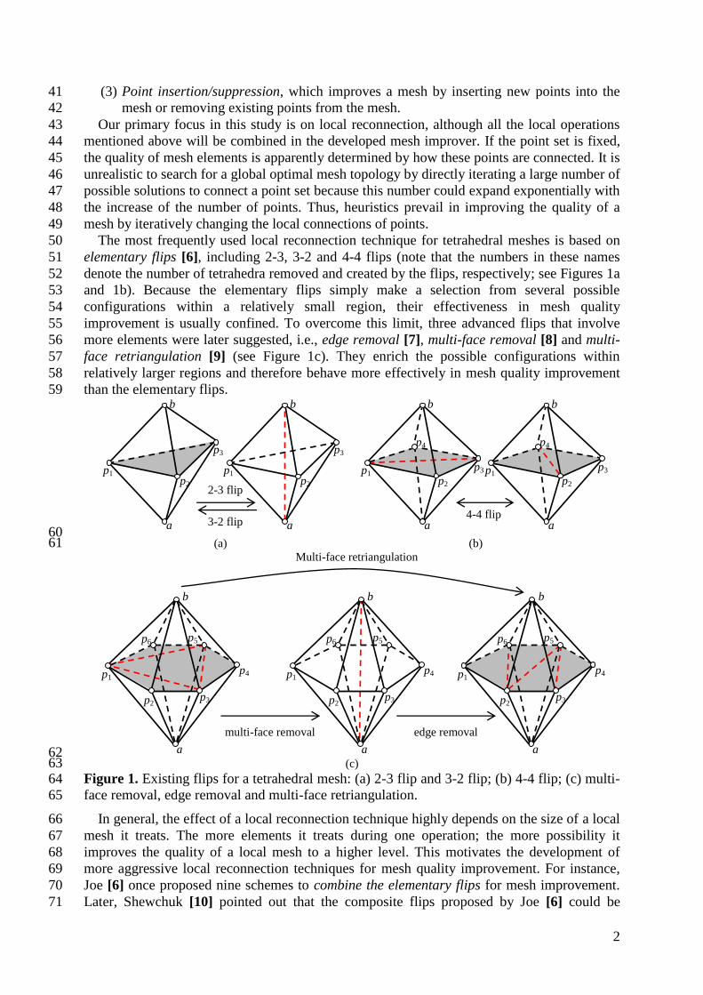
The most frequently used local reconnection technique for tetrahedral meshes is based on 50

elementary flips [6], including 2-3, 3-2 and 4-4 flips (note that the numbers in these names 51

denote the number of tetrahedra removed and created by the flips, respectively; see Figures 1a 52

and 1b). Because the elementary flips simply make a selection from several possible 53

configurations within a relatively small region, their effectiveness in mesh quality 54

improvement is usually confined. To overcome this limit, three advanced flips that involve 55

more elements were later suggested, i.e., edge removal [7], multi-face removal [8] and multi-56

face retriangulation [9] (see Figure 1c). They enrich the possible configurations within 57

relatively larger regions and therefore behave more effectively in mesh quality improvement 58

than the elementary flips. 59

60 (a) (b) 61

62 (c) 63

Figure 1. Existing flips for a tetrahedral mesh: (a) 2-3 flip and 3-2 flip; (b) 4-4 flip; (c) multi-64

face removal, edge removal and multi-face retriangulation. 65

In general, the effect of a local reconnection technique highly depends on the size of a local 66

mesh it treats. The more elements it treats during one operation; the more possibility it 67

improves the quality of a local mesh to a higher level. This motivates the development of 68

more aggressive local reconnection techniques for mesh quality improvement. For instance, 69

Joe [6] once proposed nine schemes to combine the elementary flips for mesh improvement. 70

Later, Shewchuk [10] pointed out that the composite flips proposed by Joe [6] could be 71

multi-face removal edge removal

Multi-face retriangulation

a

b

p1

p2

p3

p4

p5

p6

a

b

p1

p2

p3

p4

p5

p6

a

b

p1

p2

p3

p4

p5

p6

4-4 flip a

p4

p2

b

p1

p3

a

p4

p2

b

p1

0

p3

a

p2

b

p1

p3

a

p2

b

p1

p3

3-2 flip

2-3 flip

3

expressed as one or two edge removal operations. Thus, Shewchuk suggested that the study of 72

composite edge removal transformations was a fruitful direction for mesh improvement 73

research. Unfortunately, Shewchuk did not present details about what such composite 74

transformations are and how to implement such transformations efficiently. As a result, it was 75

observed that no composite transformations are actually incorporated into the open-source 76

tetrahedral improver (namely Stellar thereafter) developed by Klinger and Shewchuk [11, 12]. 77

The main contribution of this present study is the development of a new local reconnection 78

technique that could act like composite edge removal transformations. This technique is based 79

on the recursive callings of a new flip named shell transformation. The single calling of shell 80

transformation could be considered as an enhanced version of edge removal transformation. 81

However, an essential difference exists between two approaches, and enables shell 82

transformation to be executed recursively (see Section 2.4 for details). Thus, edge removal 83

only makes a selection from a few possible configurations within a single shell (i.e., a 84

polyhedron that can be filled up with a mesh composed of a set of elements that meet each 85

other at one common edge). However, the recursive callings of shell transformations can 86

execute a sequence of shell transformations on neighboring shells. In other words, recursive 87

shell transformations could be performed on a much larger element set than that of edge 88

removal, thereby leading the way towards a better local optimum solution. 89

Another focus of this study is about the efficient implementation of the new local 90

reconnection technique, because local reconnections need to be employed for a large number 91

of times during the entire mesh improvement workflow. The dynamic programming algorithm 92

suggested by Shewchuk for edge removal [10, 13] will be revisited at first and then further 93

enhanced to implement the basic shell transformation routine. Besides, the computing 94

efficiency of recursive callings of shell transformations is investigated carefully because the 95

number of such callings may increase exponentially when the recursive level increases. 96

Reasonable restrictions are provided to prevent inefficient recursive callings. Meanwhile, 97

several strategies are suggested to improve the efficiency. 98

Finally, the ability of the proposed local reconnection technique will be demonstrated by 99

performing various mesh improvement tasks, some of which involve millions of elements. In 100

a pipeline of producing meshes of this magnitude, mesh generation itself may only consume a 101

few seconds computing time, owing to recent advancement in the field of fast and parallel 102

mesh generation techniques [14-17]. However, a mesh improver possibly consumes many 103

minutes computing time or even longer in order to manage such a big mesh. Therefore, to 104

ensure the applicability of this newly developed mesh improver for large-scale problems, an 105

essential requirement we will take into account is the cost-effectiveness of the mesh improver, 106

i.e., the ability to balance the conflict requirements of resulting in a high-quality mesh and 107

saving computing time of mesh improvement. Following this concept, a set of existing 108

smoothing, point insertion and point suppression schemes are selected. Combining these 109

schemes with the proposed local reconnection technique, a cost-effective improver applicable 110

to large-scale meshes is therefore developed and verified. 111

The remainder of this article will be organized as follows. In Section 2, related works are 112

firstly reviewed, followed by the introduction of the new local reconnection technique in 113

Section 3. Sections 4 describes the basic implementation of shell transformation, while 114

Section 5 presents the recursive scheme of shell transformation and the local reconnection 115

scheme based on this recursive scheme. Section 6 introduces other local operations that are 116

combined to form the developed new mesh improver. Section 7 provides various examples of 117

numerical experiments demonstrating the effectiveness and efficiency of the proposed 118

scheme. Section 8 concludes with outcomes of the study. 119

4

2. RELATED WORKS 120

Firstly, related works on local reconnection techniques are reviewed in details (see Section 121

2.1). After that, a brief review on other types of local operations (see Sections 2.2 and 2.3, 122

respectively) is presented to justify our choices of these types of operations in the developed 123

mesh improver. 124

2.1 Related work on local reconnection techniques 125

Local reconnection techniques are frequently used in various circumstances of mesh 126

generation, such as Delaunay refinement [18], mesh adaptation [19], boundary recovery [1-5], 127

and mesh quality improvement [6-12, 20, 21]. The first type of local reconnection techniques 128

is based on the flips presented in Figure 1. The 3-2, 2-3 and 4-4 flips are defined as 129

elementary flips, not only because they are special cases of the advanced flips, but also 130

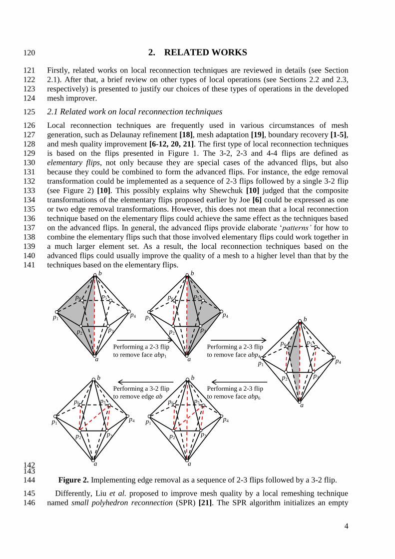
because they could be combined to form the advanced flips. For instance, the edge removal 131

transformation could be implemented as a sequence of 2-3 flips followed by a single 3-2 flip 132

(see Figure 2) [10]. This possibly explains why Shewchuk [10] judged that the composite 133

transformations of the elementary flips proposed earlier by Joe [6] could be expressed as one 134

or two edge removal transformations. However, this does not mean that a local reconnection 135

technique based on the elementary flips could achieve the same effect as the techniques based 136

on the advanced flips. In general, the advanced flips provide elaborate ‘patterns’ for how to 137

combine the elementary flips such that those involved elementary flips could work together in 138

a much larger element set. As a result, the local reconnection techniques based on the 139

advanced flips could usually improve the quality of a mesh to a higher level than that by the 140

techniques based on the elementary flips. 141

142 143

Figure 2. Implementing edge removal as a sequence of 2-3 flips followed by a 3-2 flip. 144

Differently, Liu et al. proposed to improve mesh quality by a local remeshing technique 145

named small polyhedron reconnection (SPR) [21]. The SPR algorithm initializes an empty 146

Performing a 2-3 flip

to remove face abp1 a

b

p1

p2

p3

p4

p5

p6

Performing a 2-3 flip

to remove face abp4

b

a

p1

p2

p3

p4

p5

p6

b

a

p1

p2

p3

p4

p5

p6

Performing a 2-3 flip

to remove face abp6

Performing a 3-2 flip

to remove edge ab

a

b

p2

p3

p4

p5

p6

p1

a

b

p1

p2

p3

p4

p5

p6

5

polyhedron in the neighbourhood of a poorly shaped element, and then performs an 147

exhaustive search to find the optimal tetrahedralization of this polyhedron. Typically, the 148

advanced flips treat only a local mesh composed of a few tetrahedral elements, while the SPR 149

algorithm can search for the optimal tetrahedralization of a polyhedron composed of 20-40 150

tetrahedral elements. Consequently, it was reported that the SPR algorithm could achieve a 151

better mesh improvement result than that of the flip-based algorithm [21]. However, the main 152

issue of the SPR algorithm is its computing complexity, since the problem of meshing an 153

empty polyhedron is NP hard. Although some strategies have been proposed in the past to 154

improve the timing-related performance of the SPR algorithm [4, 21], our experience shows 155

that, if the local reconnection scheme of a mesh improver is completely dependent on the SPR 156

algorithm. In addition, the runtime of a mesh improver may be beyond the user’s expectation, 157

in particular when the treated mesh is composed of one million or more elements. 158

2.2 Related work on mesh smoothing 159

The mesh smoothing methods can be classified into two categories in general, i.e., the 160

Laplacian-type method [22] and the optimization-based method [20, 23-28]. The Laplacian-161

type method moves each mesh vertex towards the center of its neighboring vertices. It 162

provides no guarantee for the improvement of mesh quality, therefore leading to either low 163

quality or even possibly invalid elements. To overcome this drawback, various optimization-164

based approaches were proposed. These approaches can be divided into two types in 165

accordance with the choice of objective functions. The local method maximizes a quality 166

function for the elements surrounding each mesh vertex by relocating mesh vertices 167

iteratively [20, 23, 24]. The global method maximizes a quality function for all elements by 168

relocating all mesh vertices simultaneously [25-28]. While the local method may improve an 169

element at a cost of degrading its neighboring elements, the global method relieves this 170

conflict to some extents by considering the quality of the entire mesh as a whole. 171

Nevertheless, because the global method needs to solve a large-scale optimization model, the 172

choice of solution methods for this optimization model will be the key step to achieve 173

acceptable computing time and performance [28]. Likewise, in the case of surface mesh 174

smoothing, various local and/or global shape-preserving approaches have been developed, in 175

which the global approach based on geometric flows is now still prevailing because of its 176

powerful ability to preserve geometric features and thus reduce volume shrinkage [25]. 177

Since the cost-effectiveness of a new mesh improver is our primary goal to achieve, we 178

select a local approach instead of a more time-consuming global approach for mesh 179

smoothing. More specifically, we combine an optimization-based algorithm [20] with the 180

Laplacian smoothing [22]. See Section 5.4 later for more details. 181

2.3 Related work on point insertion and point suppression 182

It is intuitive to eliminate low-quality elements by inserting vertices into existing meshes. 183

Typically, a new vertex can be located at the circumcenter [5, 29] or centroid of a poor 184

element [1, 4], or the midpoint of the longest edge of this element [2, 30]. One typical strategy 185

to insert this kind of vertex into a mesh is by Delaunay refinement [1-5, 29, 31], or more 186

simply, by splitting the element(s) containing the new vertex (which may result in temporary 187

low-quality elements) firstly and then improving the mesh by combining smoothing and local 188

reconnection [19]. Besides, Klingner and Shewchuk suggested an effective but very time-189

consuming point insertion scheme that combines a Delaunay-type algorithm with smoothing 190

operations [11]. It is possible that hundreds of elements are involved in just one single 191

operation. Nevertheless, to meet our goal of developing a cost-effective mesh improver for 192

large-scale problem inputs, we adopt an edge-splitting based point insertion scheme. 193

6

As a reverse operation of point insertion, it is not surprising that point suppression can also 194

improve local mesh quality by remeshing an empty polyhedron composed of all elements 195

surrounding the vertex to be removed. The challenge mainly comes from those polyhedra that 196

cannot be tetrahedralized if no Steiner points are allowed [31]. Meanwhile, even if a 197

polyhedron can be tetrahedralized without inserting Steiner points (although the prediction of 198

this is NP hard [31]), it is not easy to find an optimal mesh to fill in that polyhedron (it is also 199

NP hard [4, 21]). Theoretically, the SPR algorithm mentioned in Section 2.1 [4, 21] could be 200

a good candidate for remeshing an empty polyhedron because it can provide an optimal 201

solution when the polyhedron is meshable. Nevertheless, as we pointed earlier, the main issue 202

of the SPR algorithm is its relatively poor timing performance. Therefore, we adopt an edge-203

contraction based point suppression routine that is available from Stellar [12, 13]. 204

See Section 5.5 later for the developed point insertion and suppression schemes. 205

3. SHELL TRANSFORMATION AND ITS RECURSIVE CALLINGS: 206

THE MAIN IDEA 207

For the completeness, we have briefly reviewed different types of local operations in order to 208

justify our choices. However, it must be emphasized that the main contribution of this study is 209

the development of a new local reconnection technique. With respect to other local 210

operations, we only select a suitable operation among various existing approaches to meet our 211

goal of developing a cost-effective mesh improver. 212

Before introducing the new local reconnection technique, Figure 3 illustrates some 213

terminologies in relation with a shell structure because all of the flips discussed in this study, 214

including those presented earlier in Figure 1 and the new proposed shell transformation, will 215

involve this structure. 216

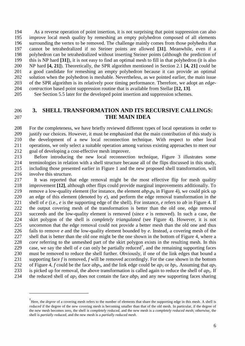
It was reported that edge removal might be the most effective flip for mesh quality 217

improvement [12], although other flips could provide marginal improvements additionally. To 218

remove a low-quality element (for instance, the element abp5p6 in Figure 4), we could pick up 219

an edge of this element (denoted by e), and perform the edge removal transformation in the 220

shell of e (i.e., e is the supporting edge of the shell). For instance, e refers to ab in Figure 4. If 221

the output covering mesh of the transformation is better than the old one, edge removal 222

succeeds and the low-quality element is removed (since e is removed). In such a case, the 223

skirt polygon of the shell is completely triangulated (see Figure 4). However, it is not 224

uncommon that the edge removal could not provide a better mesh than the old one and thus 225

fails to remove e and the low-quality element bounded by e. Instead, a covering mesh of the 226

shell that is better than the old one might be the one shown in the bottom of Figure 4, where a 227

core referring to the unmeshed part of the skirt polygon exists in the resulting mesh. In this 228

case, we say the shell of e can only be partially reduced†, and the remaining supporting faces 229

must be removed to reduce the shell further. Obviously, if one of the link edges that bound a 230

supporting face f is removed, f will be removed accordingly. For the case shown in the bottom 231

of Figure 4, f could be the face abp5, and the link edge could be ap5 or bp5. Assuming that ap5 232

is picked up for removal, the above transformation is called again to reduce the shell of ap5. If 233

the reduced shell of ap5 does not contain the face abp5 and any new supporting faces sharing 234

†Here, the degree of a covering mesh refers to the number of elements that share the supporting edge in this mesh. A shell is

reduced if the degree of the new covering mesh is becoming smaller than that of the old mesh. In particular, if the degree of

the new mesh becomes zero, the shell is completely reduced, and the new mesh is a completely reduced mesh; otherwise, the

shell is partially reduced, and the new mesh is a partially reduced mesh.

7

ab, the shell of ab is reduced as well; otherwise, a process that attempts to remove the 235

supporting faces around ap5 is repeated. 236

To better understand the above recursive scheme, Figure 5 illustrates how this scheme 237

works on a local mesh composed of two shells (see Figure 5a), aimed at removing the edge ab 238

from the mesh. Firstly, a transformation is called on the shell of ab. Since the shell cannot be 239

completely reduced, the edge ab still exists in the output mesh (see Figure 5b). Nevertheless, 240

the degree of the shell is reduced from 5 to 4. To reduce the shell further, a link edge bh is 241

picked up and a transformation is called on the shell of bh and reduces this shell completely. 242

Besides, the degree of the shell of ab is reduced from 4 to 3 after this step (see Figure 5c). 243

Finally, a transformation is called to update the shell of ab to remove ab by a single 3-2 flip 244

(see Figure 5d for the final output). 245

246

Figure 3. The terms defined for the mesh entities of a shell. 247

248

Figure 4. The difference between edge removal and a single calling of shell transformation. 249

This difference enables shell transformation to be called recursively while edge removal 250

cannot. This recursive ability is the main advantage of shell transformation technique. 251

Here, given the covering mesh of a shell, the transformation that attempts to reduce the 252

a

b

p1

p2

p3

p4

p5

p6

a

b

p1

p2

p3

p4

p5

p6

shell transformation

edge removal

a

b

p1

p2

p3

p4

p5

p6

p1

p2

p3

p4

p5

p6

p1

p2

p3

p4

p5

p6

a completely triangulated skirt

polygon

a partially triangulated skirt

polygon, where its core refers

to the quad p2p3p5p6

a

b

p1

p2

p3

p4

p5

p6

supporting edge

supporting node

supporting node

skirt node

skirt edge

link edge

supporting face skirt polygon

8

shell is denoted as shell transformation. The main difference between shell transformation 253

and edge removal is that shell transformation allows the output mesh containing a partially 254

triangulated skirt polygon while edge removal does not. If the output covering mesh of shell 255

transformation does not contain a core, shell transformation is the same operation as edge 256

removal. In this respect, edge removal could be considered a special case of shell 257

transformation. In other words, shell transformation could be considered as an enhanced 258

version of edge removal because it considers more possibility to mesh a shell. Moreover, the 259

main advantage of shell transformations is rooted in its recursive ability. As Joe have 260

demonstrated [6] that the composite transformations of elementary flips could improve the 261

quality of a mesh to a much higher level than elementary flips, and the recursive callings of 262

shell transformations, acting like composite edge removal transformations, could perform 263

much better than edge removal in most mesh improvement tasks, as we will demonstrate in 264

Section 6. 265

266 (a) (b) (c) (d) 267

Figure 5. Illustration for the recursive callings of shell transformations. (a) The input mesh. 268

(b) The output after the first shell transformation calling on the shell of ab. (c) The output 269

after the second shell transformation calling on the shell of bh. (d) The final output after the 270

third shell transformation calling on the shell of ab. 271

4. A SINGLE CALLING OF SHELL TRANSFORMATION 272

To implement a shell transformation procedure, a key step is to develop an algorithm that can 273

triangulate a skirt polygon partially. Meanwhile, among all of the valid triangulation schemes, 274

an algorithm needs to find the triangulation corresponding to an optimal covering mesh. In 275

this section, we will first reproduce a dynamic programming algorithm suggested by 276

Shewchuk [10], which can be used to triangulate the skirt polygon completely and optimally. 277

Next, the proposed shell transformation algorithm is described in details, which enhances the 278

Shewchuk’s algorithm in order to triangulate the skirt polygon partially and optimally. 279

4.1 The algorithm proposed by Shewchuk [10] 280

Given a shell covered by a set of tetrahedra 1 ( 1,2, , )i ip p ab i m , each triangulation 281

1 2 2{ , , }mt t t of the skirt polygon induces a tetrahedralization of the shell: 282

{conv( , ) conv( , ) | 1,2, , 2}i it a t b i m . 283

Here, conv( ) refers to a tetrahedron formed by a face and a node. We define the quality of 284

to be the quality of the worst tetrahedron within the tetrahedralization . 285

For each node (1 )ip i m , i mp is its alias. ,R i j defines a ring of edges whose ending 286

nodes are 287

h

c

d e

f

a

b

g

h

c

d e

f

a

b

g

h

c

d e

f

a

b

g

h

c

d e

f

a

b

g

9

1

,

1

{ , , } 1P

{ , , } 1

i i j

i j

j j i m

p p p i j m

p p p j i m

. 288

Selecting a node ,Pk i jp other than ip and jp , the triangulation of ,R i j includes three 289

parts, as shown in Figure 6: 290

, . ,T T Ti j i k k j i k jp p p . 291

We can define a matrix qM to record the quality of the optimal triangulation of ,R i j as: 292

,P , ,( , ) max min{ ( , ), ( , ), ( , , , ), ( , , , )}

k i j k i j

q q q i j k i j kp p p p

i j i k k j q a p p p q p p p b

M M M , (1) 293

where ( )q is the quality function for tetrahedral elements. ( , )q i j M when 1j i . 294

Since 1 ,i j m ( m refers to the size of the skirt polygon), we know qM is a m m 295

matrix. 296

Based on Equation 1, Algorithm 1 fills in the upper triangular part of qM by an order of 297

decreasing i and increasing j so that ( , )q i kM and ( , )q k jM are computed before 298

( , )q i jM . Meanwhile, Algorithm 1 fills in another matrix kM that records the values of k 299

that maximize Equation 1 in order to reconstruct the optimal triangulation optT : 300

opt opt

1,

opt opt opt

, , ,

T T

T T T ( ( , ))

m

i j i k k j i k j kp p p k i j

M. 301

Algorithm 1. Filling in the upper triangular part of qM and kM 302

fillInMatrices_UpRight(a, b, P, Mq, Mk)

Inputs:

a and b: the support nodes of a shell,

P = {p1, p2, …, pm}: the skirt polygon of a shell

1. for i = m – 2 downto 1

2. for j = i + 2 to m

3. for k = i + 1 to j – 1

4. q = min{q(a, pi, pk, pj), q(pi, pk, pj, b)}

5. if k < j – 1

6. q = min{q, Mq(k, j)}

7. if k > i + 1

8. q = min{q, Mq(i, k)}

9. if k = i + 1 or q > Mq(i, j)

10. Mq(i, j) = q

11. Mk(i, j) = k 303

304 Figure 6. Decomposing a triangulation optimization problem into sub-problems. 305

pi

pj

pk

Ti,j = Ti,k∪Tk,j∪△pi pk pj

Ti,k

Tk,j

pi pk pj

10

4.2 The proposed shell transformation algorithm 306

Firstly, we introduce the concept of triangulation graph. It is a directed graph defined on a 307

polygon that is bounded by a set of nodes 1 2{ , , }mp p p . A graph node corresponds to a 308

polygon node, and a graph edge ,i jp p exists if there are valid triangulations for the ring 309

,R i j . Note that qM provides a representation of the triangulation graph: ( , ) 0q i j M 310

means that there is a valid triangulation for the ring ,R i j ; thus, ,i jp p is a graph edge. 311

Algorithm 1 only fills in one half of qM and kM . To get a complete representation of 312

the triangulation graph, the lower left elements of qM and kM must be computed. 313

Algorithm 2 present a routine that fills in all of useful elements of qM and kM , which 314

could be located in either side of the main diagonal of the two matrices. In the new algorithm, 315

one diagonal of qM and kM is computed at a time in the increasing order of the size of 316

,R i j (i.e., number of vertices). Note that after calling Algorithm 2, (1, )q mM , and 317

(2,1)qM , ……, and ( , 1)q m mM all records the quality of the optimal triangulation of the 318

complete skirt polygon, but with different start and end vertices. Based on Algorithm 2, we 319

could then implement a single calling of shell transformation (see Algorithm 3), where a key 320

step is to define the core of the shell. As shown in Figure 7, the core introduced in shell 321

transformation corresponds to a simple cycle of the triangulation graph of the skirt polygon. 322

Therefore, once the graph is set up by calling Algorithms 1 and 2, all of the simple cycles are 323

visited, and the optimal one is picked up to reconstruct the triangulation of the skirt polygon 324

(i.e., Line 5 of Algorithm 3). Here, a simple cycle is identified as optimal when it corresponds 325

to an optimal covering mesh (K). Note that the definition on the optimality of a mesh could be 326

application specific, see Section 4.3 for details. 327

Algorithm 2. Filling in qM and kM 328

fillInMatrices(a, b, P, Mq, Mk)

Inputs:

a and b: the support nodes of a shell

P = {p1, p2, …, pm}: the skirt polygon of a shell

1. for d = 2 to m - 1

2. for i = 1 to m

3. j′ = i + d

4. for k′ = i + 1 to j′ – 1

5. j = j′ > m ? j′ - m : j′

6. k = k′ > m ? k′ - m : k′

7. q = min{q(a, pi, pk, pj), q(pi, pk, pj, b)}

8. if k′ < j′ – 1

9. q = min{q, Mq(k, j)}

10. if k′ > i + 1

11. q = min{q, Mq(i, k)}

12. if k′ = i + 1 or q > Mq(i, j)

13. Mq(i, j) = q

14. Mk(i, j) = k 329

Assuming that the node set of the core is 1 1 1{ , , }n nc c c c cp p p p , the reconstructed 330

triangulation is (see Figure 7): 331

11

1

opt opt

,T {T | 1,2, , }j jc c j n

332

The new covering mesh of the shell is: 333

1

1 2

1

2

{conv( , ) conv( , ) | T }

{tetr( , , , ) | 1,2, , }j j

opti i i

c c

t a t b t

p p a b j n

, (2) 334

where tetr( ) refers to the tetrahedral element formed by four specified nodes. 335

Algorithm 3. A general routine of shell transformation 336

shellTransformation(a, b, P, Kold)

Inputs:

a and b: the support nodes of the shell

P = {p1, p2, …, pm}: the skirt polygon of the shell

Kold: the old covering mesh of the shell

1. fillInMatrices_UpRight(a, b, P, Mq, Mk)

2. fillInMatrices_LowLeft(a, b, P, Mq, Mk)

3. G: the triangulation graph with Mq as its matrix representation

4. Pc: an optimal simple cycle of G

5. Topt

: the reconstructed triangulation from Pc, see Figure 6

6. K: the new covering mesh of the shell, see Equation 2

7. if K ≠ and K ≠ Kold

8. Remesh the shell by replacing Kold with K 337

338 Figure 7. Illustration for the triangulation graph of a polygon, where those lines with arrows 339

are a group of graph edges, forming a simple cycle and thus defining a scheme that 340

triangulates the polygon partially. 341

5. RECURSIVE CALLINGS OF SHELL TRANSFORMATIONS 342

5.1 The basic routine 343

A single shell transformation calling only involves a small number of elements. It may not be 344

able to reduce a shell completely because of the constraints on the shell boundaries. Hence, 345

we develop a routine that calls shell transformations recursively to remove these constraints. 346

Algorithm 4 details the routine of recursive shell transformations. Given an edge e, the 347

calling recursiveST(e, , 0, lmax) attempts to remove the edge e, where lmax limits the 348

ncp

1 1( )

nc cp p

2cp

3cp

&a b

1,Tn nc c

1 2,Tc c

2 3,Tc c

12

maximally allowed recursive level. Given a face f and one of its boundary edges e, the calling 349

recursiveST(e, f, 0, lmax) attempts to remove the face f. 350

Note that Algorithm 4 expands an edge tree, where the input edge e is the root of this tree, 351

and those link edges (e′) inputted for further recursions are children of the edge e. In this 352

manner, the tree can be expanded recursively. If a tree node v1 is an ancestor of another tree 353

node v2, we say the edge corresponding to v1 is an ancestor edge of the edge corresponding to 354

v2. 355

5.2 Termination and efficiency 356

Two routines called by Lines 10 and 3 account for the timing-related performance of 357

Algorithm 4, namely pickRecursiveLinkEdge and shellTransformation. They determine 358

how many shell transformations are executed and how fast a single shell transformation can 359

run, respectively. 360

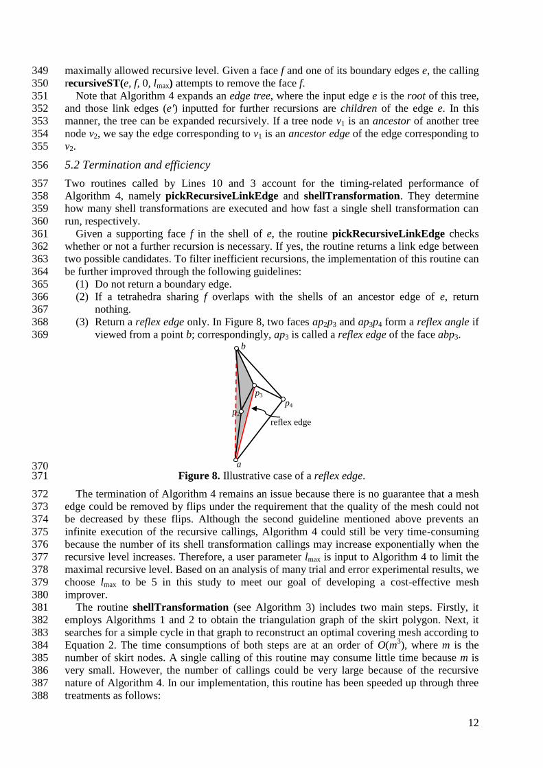
Given a supporting face f in the shell of e, the routine pickRecursiveLinkEdge checks 361

whether or not a further recursion is necessary. If yes, the routine returns a link edge between 362

two possible candidates. To filter inefficient recursions, the implementation of this routine can 363

be further improved through the following guidelines: 364

(1) Do not return a boundary edge. 365

(2) If a tetrahedra sharing f overlaps with the shells of an ancestor edge of e, return 366

nothing. 367

(3) Return a reflex edge only. In Figure 8, two faces ap2p3 and ap3p4 form a reflex angle if 368

viewed from a point b; correspondingly, ap3 is called a reflex edge of the face abp3. 369

370 Figure 8. Illustrative case of a reflex edge. 371

The termination of Algorithm 4 remains an issue because there is no guarantee that a mesh 372

edge could be removed by flips under the requirement that the quality of the mesh could not 373

be decreased by these flips. Although the second guideline mentioned above prevents an 374

infinite execution of the recursive callings, Algorithm 4 could still be very time-consuming 375

because the number of its shell transformation callings may increase exponentially when the 376

recursive level increases. Therefore, a user parameter lmax is input to Algorithm 4 to limit the 377

maximal recursive level. Based on an analysis of many trial and error experimental results, we 378

choose lmax to be 5 in this study to meet our goal of developing a cost-effective mesh 379

improver. 380

The routine shellTransformation (see Algorithm 3) includes two main steps. Firstly, it 381

employs Algorithms 1 and 2 to obtain the triangulation graph of the skirt polygon. Next, it 382

searches for a simple cycle in that graph to reconstruct an optimal covering mesh according to 383

Equation 2. The time consumptions of both steps are at an order of O(m3), where m is the 384

number of skirt nodes. A single calling of this routine may consume little time because m is 385

very small. However, the number of callings could be very large because of the recursive 386

nature of Algorithm 4. In our implementation, this routine has been speeded up through three 387

treatments as follows: 388

a

b

p2

p3

p4

reflex edge

13

(1) Introduce the validity conditions (see Section 4.3) in the first step to simplify the 389

triangulation graph; 390

(2) Search for the optimal simple cycle first to prevent those unnecessary searches for low-391

quality cycles; 392

(3) Record the results of time-consuming mesh validity and quality computations after 393

they are executed for the first time so that simple queries can replace the repeated 394

callings of these computations. 395

Algorithm 4. The routine of recursive shell transformations 396

recursiveST(e, f, l, lmax)

Inputs:

the supporting edge, denoted e

a face containing e that the routine attempts to remove, denoted f

the recursive level with an initial value of zero, denoted l

the maximally allowed recursive level, denoted lmax

Variables:

the ending nodes of an edge, denoted a(·) and b(·)

the skirt polygon of the shell of an edge, denoted P(·)

the set of elements containing an edge, denoted S(·)

a set of link faces contained in S(·), denoted F(·) = { f1′, f2′, …, fm′}, where m = |F(·)|

1. if | S(e)| <= 0 or (f != and f F(S(e)))

2. return success

3. shellTransformation(a(e), b(e), P(e), S(e))

4. if | S(e)| <= 0 or (f != and f F(S(e)))

5. return success

6. if l >= lmax /* the resursive level is limited under lmax. */

7. return fail

8. m = |S(e) | /* record the size of the shell S(e) */

9. for i = 1 to m

10. e′ = pickRecursiveLinkEdge(fi′) /* filters are set to avoid inefficient recursions */

11. if e′ !=

12. recursiveST(e′, fi′, l+1, lmax) /* recursive calling */

13. if |S(e) | < m /* S(e) is reduced as well */

14. retrun recursiveST(e, f, l, lmax) /* recursive calling */

15. return fail 397

Another factor that affects the efficiency of Algorithm 4 is the routine that identifies a shell 398

in the input mesh (referring to the shell-find routine thereafter), which is employed by Lines 4 399

and 13 of Algorithm 4. The efficiency of this routine depends on the data structure adopted to 400

represent a tetrahedral mesh. In our scheme, four incident vertices are stored for each 401

tetrahedron, plus four neighboring elements of this tetrahedron. Meanwhile, for each mesh 402

vertex, one element incident to this vertex is stored. This data structure requires a small 403

amount of memories, and the shell-find routine based on it only needs to traverse the elements 404

locally. Given two ending vertices of an edge (denoted by v1 and v2, respectively), the shell-405

find routine is separated into two phases. In the first phase, one element that contains the input 406

edge is searched by the following steps: 407

(1) Get the stored element incident to v1 and push it into a stack; 408

(2) If the stack is empty, exit the routine and return NULL; otherwise, remove the top 409

14

element from the stack and go to Step 3; 410

(3) If the top element contains v2, return the top element and exit the routine; 411

(4) Flag the top element as visited, and then visit its neighboring elements. For any 412

unvisited neighbor, if it contains v1 as well, push it into the stack; 413

(5) Go back to Step 2. 414

If no valid element is returned by the above procedure, the shell is empty; otherwise, 415

starting from the returned element, the entire shell can be visited by using the neighboring 416

indices of elements. In the worst scenarios, the first phase visits all elements surrounding v1, 417

and the number of such elements is close to 30 on average for real mesh examples. The 418

second phase visits all elements surrounding the edge, and the number of such elements is 419

about 5-7 on average‡. Therefore, the first phase dominates a general calling of the routine in 420

terms of computing time. However, in many circumstances, one element surrounding an edge 421

is stored somewhere before calling the shell-find routine. By using this element as an extra 422

input, the timing-related performance of the shell-find routine can be improved remarkably by 423

skipping over the first phase. 424

5.3 Validity and optimality conditions. 425

The shell transformation routine presented in Algorithm 3 needs to output an optimal 426

covering mesh of a shell among all valid ones. Here, the definitions of validity and optimality 427

depend on specific application purposes. For mesh quality improvement, three types of 428

validation conditions are set for covering meshes as: 429

(1) The basic condition, which requires all elements have positive volumes. 430

(2) The recursive condition, which requires each shell transformation should create no 431

supporting faces around any ancestor edge of the current supporting edge. 432

(3) The application specific condition, in the context of mesh improvement, which requires 433

the quality of the output covering mesh of the shell should be higher than the quality of 434

the input covering mesh. 435

It is possible that more than one valid covering mesh exists for a shell. The final output of a 436

shell transformation calling is the covering mesh with the highest possible quality. See 437

Section 5.1 for the definition of mesh quality. 438

5.4 The shell transformation based local reconnection scheme 439

If one edge or face of a low-quality element is removed, the element will be removed 440

accordingly. Based on this concept, Algorithm 5 presents a local reconnection scheme that 441

attempts to remove low-quality elements by removing the edges or faces of these elements. 442

All of low-quality elements are stored in a heap in an ascending order of the element 443

quality. Firstly, Algorithm 4 is called on an edge of the first element of the heap. If the 444

element is removed by Algorithm 4, Algorithm 4 succeeds; otherwise, Algorithm 4 is 445

repeated on another edge of the element until all edges of the element are attempted. To 446

protect the mesh boundary, the edges attempted for removal must be interior edges of the 447

mesh. Next, if Algorithm 4 fails to remove the element, we attempt to remove the faces of this 448

element individually. To protect the mesh boundary, the faces attempted for removal must be 449

interior faces of the mesh. The 2-3 flip shown in Figure 1a is the simplest local scheme for 450

face removal. However, a more effective alternative is multi-face removal (see Figure 1c). 451

‡ It is worth noting that both numbers could vary case by case, depending on mesh topologies. Nevertheless, the meshes

considered in this study are inputs for numerical simulations, where only a small percentage of elements are badly shaped.

For different meshes of this type, it is observed that both numbers usually remain within the ranges we mentioned in the text.

For instance, for the unimproved F16 and Bridge meshes to be presented in Section 7 for tests, the average numbers of

elements surrounding interior mesh nodes are both 5.50. After mesh improvement, these two numbers are reduced to 5.21

and 5.20 respectively. The numbers of elements surrounding interior mesh edges are 26.05 and 26.21, respectively. After

mesh improvement, these two numbers are reduced to 23.82 and 23.80 respectively.

15

Shewchuk [10] suggested an implementation of multi-face removal. In this study, we present 452

an alternative solution based on the proposed shell transformation routine (i.e., Algorithm 3). 453

Given an interior face f for removal, the proposed algorithm takes the following steps as: 454

(1) Find two tetrahedra sharing face f, and denote the apexes of the tetrahedra opposite to f 455

as a and b, respectively. 456

(2) Find all of the faces opposite to a and b. As shown in Figure 9a, these faces may form 457

several connected components. 458

(3) Select a component that includes the face (or faces) intersected by ab, as shown in 459

Figure 9b. 460

(4) Define the boundary of the selected component as a polygon. If a point (such as p7 in 461

Figure 9c) is contained in the interior of the polygon, remove one face (such as the face 462

p1p2p7 in Figure 9c) incident on this point from the component. 463

(5) Now we get a local mesh like the one shown in the left of Figure 1c. With this mesh as 464

the input, the shell transformation routine (i.e., Algorithm 3) is called to search for a 465

better covering mesh to fill in the shell region. 466

To avoid an infinite execution of the loop defined in Lines 2-16 of Algorithm 5, no matter 467

the element for removal is removed or not, this element must be removed from the heap 468

before the next iteration. 469

Algorithm 5. The combinational edge removal based on recursive shell transformation 470

localReconnection(M, lmax)

Inputs:

the mesh to be improved, denoted M

the maximally allowed recursive level, denoted lmax and the default value is 5

Variables:

the heap that stores all of low-quality elements, Tbad

1. Insert all of low-quality elements into Tbad in the ascending order of the element quality

2. while Tbad is not empty

3. t: the first element of Tbad

4. If t has been removed from M

5. goto line 16

6. E = {e1, e2, …, en}: the set of edges of t qualified for removal (n <= 6)

7. for j = 1 to n

8. recursiveST(ej, , 0, lmax)

9. if t is removed

10. goto line 16

11. F = {f1, f2, …, fm}: the set of faces of t qualified for removal (m <= 4)

12. for j = 1 to m

13. Remove fj by a shell transformation based multi-face removal routine

14. if t is removed

15. break

16. Remove t from Tbad 471

472

16

473 (a) 474

475 (b) (c) 476

Figure 9. The procedure that prepares the inputs for the multi-face removal operation. 477

6. THE OVERALL MESH IMPROVEMENT ALGORITHM 478

The application goal of this study is to develop a cost-effective mesh improver. In this 479

section, we first present some basic considerations that guide this development procedure. 480

Then, we introduce the set of smoothing, point insertion and point suppression schemes 481

incorporated in our mesh improver. Finally, the overall mesh improvement scheme is detailed. 482

6.1. The basic considerations 483

In this study, the minimum sine of dihedral angles is used as a default quality measure. The 484

quality measure of a mesh is evaluated by a vector listing the quality of each tetrahedron 485

contained by the mesh, in an order from the worst to the best. Since the worst tetrahedron in a 486

mesh has far more influence than those average tetrahedra, the quality vectors of two meshes 487

are compared lexicographically so that, for instance, an improvement in the second-worst 488

tetrahedron improves the overall mesh quality even if the worst tetrahedron has not changed. 489

To ensure the heuristic algorithm never worsens the quality of a mesh, a hill-climbing 490

method is adopted in all of the developed local schemes, which considers applying a local 491

operation only if the quality of the changed mesh will be better than that of the original mesh. 492

Local operations that do not improve the mesh quality are not applied. The method stops 493

when no operation can achieve further improvement (i.e., the mesh is already locally optimal), 494

or when a further optimization promises too little gain. 495

Meanwhile, since the focus is usually on the worst tetrahedron, only bad elements are 496

treated to save the computing time, which refer to those elements whose minimum sine values 497

are less than 0.5 in the following discussions, i.e., at least one dihedral angle of the element is 498

either below 30° or above 150°. 499

The surface boundary of a volume mesh influences the mesh quality considerably. In the 500

applications where the boundary can be changed to some extents, it is beneficial to extend the 501

local schemes for mesh quality improvement from interior mesh entities to boundary entities. 502

a&b

p1

p2

p3

p4

p5

p6

p7

a&b

p1

p2

p3

p4

p5

p6

p7

b

a

p1

p2

p3

p4

p5

p6

p7

p8

p9

p10

a&b

p1

p2

p3

p4

p5

p6

p7

p8

p9

p10

17

However, in many applications, the improved mesh need to be consistent with a CAD model 503

or matched face-to-face with another mesh. To limit the discussions, the presented algorithm 504

regards the boundary configuration of the mesh as untouchable, i.e., vertices on the boundary 505

cannot be smoothed, and the connectivity between them cannot be changed. 506

6.2. Smoothing 507

To achieve the cost-effectiveness, we combine an optimization-based algorithm [20] with the 508

Laplacian smoothing to reposition each interior mesh point that is included by at least one bad 509

element (referred to as a bad point hereafter): 510

(1) Perform Laplacian smoothing. If the improved ball (referring to all of elements incident 511

on the point) contains no bad elements, the smoothing succeeds; otherwise, continue. 512

(2) Perform the optimization-based smoothing. 513

To save the smoothing time, a mesh point is flagged as smoothed after a successful 514

smoothing, and this flag is flushed only if the ball of the point is changed. In each smoothing 515

cycle, all of non-smoothed bad points are treated only once. 516

In each smoothing pass, the smoothing cycle is repeated until three indicators of the mesh 517

quality are not improved further: (1) the quality of the worst tetrahedral (qworst); (2) the 518

number of bad elements (nbad); and (3) the average quality of bad elements (qaver). 519

6.3. Point insertion and point suppression 520

We adopt an edge-splitting based point insertion scheme. It attempts to insert a point at the 521

middle of an interior edge and then to split those elements that meet at this edge; see Figure 522

10a. Finally, the new point is smoothed, and if the resulting mesh is better than the old one, 523

the mesh will be changed; otherwise, the old mesh is restored. 524

Besides, our mesh improver relies on an edge contraction operation to remove bad points 525

of the mesh. Figure 10b illustrates this operation using a 2D example. Each edge ended with 526

the point to be suppressed is contracted to the other endpoint, and the resulting mesh 527

configuration with the best quality is selected for further smoothing. To save computing time, 528

only the point that replaces the contracted edge is smoothed. The point suppression operation 529

fails if edge contraction (plus point smoothing) cannot produce a better mesh than the old one. 530

Since only bad elements are targeted, those edges included by bad elements are attempted 531

only once in each point suppression or insertion pass. 532

533 (a) (b) 534

Figure 10. Illustration for the (a) edge splitting and (b) edge contraction operations. 535

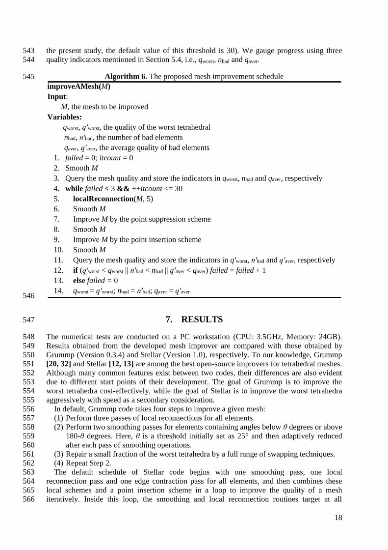
6.4. The mesh improvement schedule 536

Algorithm 6 presents the proposed mesh improvement schedule, which combines different 537

local schemes to improve the mesh quality. This schedule begins with a smoothing pass, and 538

then executes the main loop of mesh improvement. In the main loop, a smoothing pass is 539

followed after the pass of each type of topological transformations to improve the mesh 540

quality further. The main loop is ended when three subsequent combinational passes fail to 541

make sufficient progress or the number of iteration steps exceeds a predefined threshold (in 542

Edge splitting Edge contraction

18

the present study, the default value of this threshold is 30). We gauge progress using three 543

quality indicators mentioned in Section 5.4, i.e., qworst, nbad and qaver. 544

Algorithm 6. The proposed mesh improvement schedule 545

improveAMesh(M)

Input:

M, the mesh to be improved

Variables:

qworst, q′worst, the quality of the worst tetrahedral

nbad, n′bad, the number of bad elements

qaver, q′aver, the average quality of bad elements

1. failed = 0; itcount = 0

2. Smooth M

3. Query the mesh quality and store the indicators in qworst, nbad and qaver, respectively

4. while failed < 3 && ++itcount <= 30

5. localReconnection(M, 5)

6. Smooth M

7. Improve M by the point suppression scheme

8. Smooth M

9. Improve M by the point insertion scheme

10. Smooth M

11. Query the mesh quality and store the indicators in q′worst, n′bad and q′aver, respectively

12. if (q′worst < qworst || n′bad < nbad || q′aver < qaver) failed = failed + 1

13. else failed = 0

14. qworst = q′worst; nbad = n′bad; qaver = q′aver 546

7. RESULTS 547

The numerical tests are conducted on a PC workstation (CPU: 3.5GHz, Memory: 24GB). 548

Results obtained from the developed mesh improver are compared with those obtained by 549

Grummp (Version 0.3.4) and Stellar (Version 1.0), respectively. To our knowledge, Grummp 550

[20, 32] and Stellar [12, 13] are among the best open-source improvers for tetrahedral meshes. 551

Although many common features exist between two codes, their differences are also evident 552

due to different start points of their development. The goal of Grummp is to improve the 553

worst tetrahedra cost-effectively, while the goal of Stellar is to improve the worst tetrahedra 554

aggressively with speed as a secondary consideration. 555

In default, Grummp code takes four steps to improve a given mesh: 556

(1) Perform three passes of local reconnections for all elements. 557

(2) Perform two smoothing passes for elements containing angles below θ degrees or above 558

180-θ degrees. Here, θ is a threshold initially set as 25° and then adaptively reduced 559

after each pass of smoothing operations. 560

(3) Repair a small fraction of the worst tetrahedra by a full range of swapping techniques. 561

(4) Repeat Step 2. 562

The default schedule of Stellar code begins with one smoothing pass, one local 563

reconnection pass and one edge contraction pass for all elements, and then combines these 564

local schemes and a point insertion scheme in a loop to improve the quality of a mesh 565

iteratively. Inside this loop, the smoothing and local reconnection routines target at all 566

19

elements, but the most passes of edge contraction and point insertion routines target at 567

elements with angles below 40° or above 140° except for a so-called desperation pass, which 568

targets at the worst 3.5% of tetrahedra. 569

570 (a) (b) (c) 571

572 (d) (e) 573

Figure 11. The selected meshes: (a) Tire; (b) Patient-organs02; (c) The F6 aircraft; (d) The 574

F16 aircraft; (e) The London Tower bridge. Surface meshes and grid sources for mesh sizing 575

control are displayed in both graph (c) and graph (d), and the surface mesh and inviscid flow 576

simulation results induced by a crosswind are displayed in graph (e), respectively. 577

As shown in Figure 11, five meshes are selected. The first two meshes are accessible from 578

the internet: the initial mesh of tire was ever analysed in literatures [20] and [32], and 579

included in the package of Grummp [32] and Stellar [13], and the initial mesh of patient-580

organs02 is obtained from the AIM@SHAPE repository [33]. The last three meshes are 581

generated by our in-house codes following the same schedule as: 582

(1) Input a geometry model. 583

(2) Triangulate the surface by an advancing front technique. 584

(3) Tetrahedralize the volume by a Delaunay mesher [4]. 585

The original geometry models of the last three examples are all accessible from the internet. 586

The London Tower Bridge model (referred to as bridge hereafter) and the DLR-F6 wing-587

body-nacelle-pylon aircraft model (referred to as F6 hereafter) are the selected test case 588

geometries for the meshing contest session of the 23rd International Meshing Roundtable 589

(IMR) and the 2nd AIAA CFD Drag Prediction Workshop, respectively. The F16 aircraft 590

model (referred to as F16 hereafter) is obtained from GrabCAD [34]. 591

Table 1 lists the initial mesh size statistics and the mesh quality data of those selected 592

examples, where θmin and θmax refer to the minimum and maximum dihedral angles, and λ 593

refers to the percentage of bad dihedral angles, i.e., angles within the range of [0, 30°] or 594

[150°, 180°], respectively. Meanwhile, λi (i=1-5) is used to evaluate the distributions of bad 595

angles, which refers to the percentage of dihedral angles within the range of [6(i-1), 6i) or 596

(180-6i, 180-6(i-1)] degrees. For instance, λ2 refers to the percentage of dihedral angles within 597

the range of 6° to 12° or 168° to 174°. 598

20

Table 1. The initial mesh size statistics and mesh quality data. 599

Examples #tetra. #points θmin

(°)

θmax

(°)

% of bad

angles (λ)

Distribution of bad angles (%)

λ1 λ2 λ3 λ4 λ5

Tire 11,098 2,570 0.66 178.88 4.58 0.12 0.46 0.77 1.28 1.96

Patient-organs02 280,911 51,124 2.89 175.23 7.65 0.0072 0.21 1.20 2.45 3.78

F6 1,023,532 172,664 2.6e-13 ≈180 6.65 0.23 0.68 1.19 1.82 2.73

F16 18,065,336 2,906,056 2.6e-14 ≈180 6.63 0.23 0.67 1.18 1.82 2.74

Bridge 37,772,656 6,205,571 2.1e-13 ≈180 6.72 0.23 0.68 1.19 1.85 2.77

In the first test, the performance data of different local reconnection schemes are compared 600

with each other. Stellar code executes edge removal and multi-face removal routines 601

repeatedly to improve mesh topology, while Grummp code executes 2-3 flips and edge 602

removal routines repeatedly. We improve the five initial meshes by performing one pass of 603

the three local reconnection schemes, respectively. Instead of improving all elements, only 604

bad elements are treated in this test. Table 2 presents the mesh quality and the computing time 605

data comparison. 606

For patient-organs02, F6 and F16 cases, our scheme not only achieves the lowest 607

percentage of bad angles (λ), but also narrows the ranges of dihedral angles to the largest 608

extent. For bridge case, our scheme also achieves the lowest λ; however, all of the three local 609

reconnection schemes fail to improve both the smallest and the largest angles to an acceptable 610

level, although the values achieved by our scheme are slightly better. For tire case, Grummp 611

code improves θmin and θmax at the same level as our scheme. Meanwhile, Grummp code 612

achieves a slightly better value of λ than our scheme, while our scheme achieves smaller 613

values of λ1 and λ2. We believe that, for this mesh, more angles between 12° and 30° (or 614

between 150° and 168°) are generated when our scheme attempts to remove small angles 615

between 0° and 12° or large angles between 168° and 180°, because the cost of improving the 616

worst angle is possibly increased considerably due to the generation of more undesirable 617

small/large angles. 618

In this test, Stellar code achieves the best performance with respect to the computational 619

time, while Grummp code performs rather well for small meshes but very poor for big 620

meshes. For our scheme, one pass of the proposed local reconnection scheme consumes more 621

time than its counterpart in Stellar code, because of its recursive nature. Nevertheless, since 622

the proposed scheme produces a much better mesh, this marginally more time consumption is 623

acceptable. 624

Table 2. The mesh quality and computational time data for different local reconnection 625

schemes. 626

Examples #tetra. θmin

(°)

θmax

(°) λ

Distribution of bad angles (%)

Time (s) λ1 λ2 λ3 λ4 λ5

Tire

Grummp 11,019 3.36 172.38 4.21 0.069 0.30 0.57 1.18 2.09 0.09

Stellar 10,936 3.00 172.38 4.23 0.056 0.31 0.59 1.23 2.05 0.07

Present 10,906 3.36 172.38 4.42 0.047 0.27 0.61 1.30 2.19 0.21

Patient-

organs02

Grummp 265,086 5.68 165.38 3.46 6.3e-5 3.3e-3 0.12 0.96 2.37 2.6

Stellar 261,485 6.55 167.70 2.98 0 2.4e-3 0.089 0.79 2.09 2.6 Present 259,959 11.21 162.59 2.81 0 6.4e-5 0.034 0.67 2.10 5.9

F6

Grummp 955,584 0.78 178.4 0.75 3.0e-4 2.0e-3 0.016 0.10 0.63 9.8

Stellar 951,623 0.73 178.7 0.58 3.7e-4 4.3e-3 0.022 0.094 0.46 4.6 Present 946,534 3.69 174.85 0.31 7.0e-5 4.8e-4 2.5e-3 0.018 0.29 5.7

F16

Grummp 16,854,123 2.4e-4 ≈180 0.74 3.9e-4 2.3e-3 0.018 0.11 0.61 258.0

Stellar 16,791,528 1.3e-4 ≈180 0.57 9.5e-4 4.7e-3 0.024 0.097 0.45 72.6

Present 16,682,773 3.80 174.20 0.31 1.9e-5 4.1e-4 4.1e-3 0.025 0.28 85.3

Bridge

Grummp 35,233,789 3.0e-5 ≈180 0.81 2.5e-4 2.0e-3 0.017 0.11 0.67 542

Stellar 35,081,252 9.2e-5 ≈180 0.62 4.0e-4 3.8e-4 0.022 0.10 0.50 160.8

Present 34,853,521 8.6e-4 ≈180 0.36 1.5e-5 1.6e-4 1.9e-3 0.025 0.33 192.2

In the second test, we compare the default schedules of Grummp code, Stellar code and the 627

21

proposed algorithm (i.e., Algorithm 6). In this test, the option that prohibits the change on the 628

mesh surface is enabled for both Grummp and Stellar codes. In addition, because the first pass 629

of edge contraction in Stellar code can coarsen the input mesh dramatically, this pass is thus 630

disabled in this test. 631

Table 3 presents the mesh quality and computational time data from the second test. In all 632

of the cases, Grummp code outputs the worst quality meshes. For F16 and bridge cases, the 633

meshes output by Grummp code contain extremely small and/or large angles, while Stellar 634

code and our algorithm can improve them to an acceptable level for further numerical 635

simulations. We believe that the following facts might account for the relatively poor 636

performance of Grummp code. Firstly, Grummp code does not incorporate any point 637

suppression and point insertion schemes. In practice, these two schemes are useful for 638

eliminating extreme small and/or large angles of a mesh. Secondly, Grummp code only 639

executes a fixed number of passes of swapping and smoothing operations. In both Stellar code 640

and our algorithm, the adopted scheduling strategies that combine local mesh improvement 641

schemes are far more aggressive. 642

Table 3. The mesh quality and computational time data of the default schedules of Grummp, 643

Stellar and our improved method. 644

Examples #tetra. #points θmin

(°) θmax

(°) λ

Distribution of bad angles (%) Time

(s) λ1 λ2 λ3 λ4 λ5

Tire

Grummp 11,039 2,570 13.67 158.55 1.7 0 0 0.030 0.21 1.47 0.5

Stellar 10,973 2654 23.4 148.1 0.15 0 0 0 0.017 0.13 106 Present 11,840 2,751 20.67 157.45 0.26 0 0 0 0.018 0.24 1.0

Patient

-organs02

Grummp 264,954 51,124 8.93 160.40 2.91 0 1.3e-4 1.6e-3 0.06 2.85 21

Stellar 227,775 46,237 31.7 141.58 0 0 0 0 0 0 3,220 Present 266,631 52,392 20.52 149.93 8.3e-3 0 0 0 3.8e-4 7.9e-3 16

F6

Grummp 955,512 172,664 0.78 178.4 0.65 1.7e-4 3.0e-4 1.1e-3 3.5e-3 0.65 43

Stellar 918,434 171,912 18.2 158.7 5.9e-3 0 0 0 4.7e-4 5.4e-3 1,193

Present 935,608 172,167 10.64 159.79 0.017 0 5.3e-5 3.2e-4 1.4e-3 0.015 26

F16

Grummp 16,854,105 2,906,056 2.4e-4 179.99 0.63 1.5e-4 3.2e-4 2.6e-3 0.010 0.62 884

Stellar 16,360,678 2,910,076 3.8 174.2 0.027 6.1e-6 3.1e-6 1.1e-4 9.1e-4 0.026 9,882

Present 16,666,517 2,923,840 3.8 174.2 0.013 6.0e-6 1.3e-5 7.7e-5 1.2e-3 0.012 522

Bridge Grummp 35,233,695 6,205,571 3.0e-5 179.99 0.71 1.1e-4 2.0e-4 8.6e-4 6.8e-3 0.70 1,521 Stellar 34,188,981 6,211,120 7.5 171.5 0.13 0 1.0e-4 4.2e-4 9.5e-4 0.13 21,779

Present 33,698,234 6,091,180 5.79 172.55 0.13 9.9e-7 7.0e-5 4.0e-4 1.9e-3 0.13 1,412

In the second test, Stellar code outputs the best quality meshes in most occasions, and it not 645

only narrows the range of dihedral angles at most, but also reduces the percentage of bad 646

angles as well. For instance, for patient-organs02, Stellar code improves the smallest and the 647

largest angles to be 31.7° and 141.6°, respectively. In other words, the improved mesh does 648

not contain any bad angles. The mesh improved by our algorithm is slightly worse, which 649

contains 132 angles below 30° (of which 6 angles below 24°), but no angles above 150°. For 650

F16 and bridge cases, the quality levels of the improved meshes by Stellar code and our 651

algorithm are very close. 652

With respect to the computational time performance, the proposed algorithm performs the 653

best in most cases, apart from the improvement of the mesh tire. For this smallest mesh, 654

Grummp code performs the best in terms of the timing performance. Here, we define a 655

velocity index to evaluate the timing performance as: 656

v = the number of elements contained in the input mesh / the total computing time. 657

For those three inputs produced by the Delaunay mesher, i.e., F6, F16 and bridge, Stellar 658

code runs at a speed of 45.9, 18.9 and 15.4 times slower than that of the proposed algorithm, 659

respectively. It is worth noting that the adopted Delaunay mesher runs very fast. For instance, 660

the generation of the initial mesh of bridge consumes only 174 seconds, while the proposed 661

algorithm can improve it to an acceptable mesh quality level for simulations in about 1,412 662

seconds. However, if replacing the proposed algorithm by Stellar code, it will take about 6 663

22

hours to achieve only marginal improvement (compared with our results) in terms of the mesh 664

quality. In this respect, the proposed algorithm is undoubtedly a more cost-effective choice 665

than the current default schedule of Stellar code. 666

To demonstrate the performance difference between three mesh improvers more clearly, 667

Figure 12a compares the distributions of bad angles of three F16 meshes produced by 668

Grummp code, Stellar code and our mesh improver. By default, each curve contains 10 data 669

points, and the λ value of the ith point refers to the percentage of bad dihedral angles within 670

the range of [3(i-1), 3i) or (180-3i, 180-3(i-1)] degrees (i=1-10). Nevertheless, because the 671

meshes produced by Stellar code and our mesh improver contains no angles below 3° or 672

above 177°, their corresponding curves contains no data points referring to angles within this 673

range. Besides, Figure 12b compares the timing performance of three mesh improvers for five 674

test meshes of various sizes, evaluated by the velocity indices of these improvers mentioned 675

previously. 676

The λ value of each data point of the curve for Grummp code is found larger than its 677

counterparts from Stellar code and our mesh improver by nearly one or two orders of 678

magnitude, while the λ values of data points of the curves for Stellar code and our mesh 679

improver are comparable in general. However, the velocity indices of Stellar code are lower 680

than their counterparts of Grummp code and our mesh improver by one or two orders of 681

magnitude, while the velocity indices of Grummp code and our improver is at the same order. 682

From the above analysis, we can conclude that our mesh improver presented in this study can 683

achieve an overall better balanced performance between the mesh quality and computational 684

time than other two state-of-the-art algorithms, and it is therefore more suitable for the quality 685

improvement tasks involving large-scale meshes. 686

It needs to be pointed out that the initial mesh of patient-organs02 actually contains interior 687

constraints. However, because the current versions of Grummp and Stellar codes provide no 688

options to input a mesh with interior constraints, all of the tests presented above choose not to 689

respect interior constraints. In fact, the proposed algorithm can respect interior constraints 690

very well. To demonstrate this, Figure 13 compares the meshes improved by the proposed 691

algorithm with or without interior constraints. Not surprisingly, the quality of the improved 692

mesh that respects interior constraints is slightly worse. 693

694 (a) (b) 695

Figure 12. A comparison of Grummp, Stellar and our improver in terms of mesh quality and 696

timing performance. (a) The distributions of bad angles of the F16 meshes produced by three 697

improvers. (b) The velocity indices of three improvers for five test meshes. 698

23

699

Figure 13. A comparison of the improved meshes of patient-organs02 by the proposed 700

algorithm with interior constraints respected or not. In graphs (a) and (b), the blue triangles 701

are boundary triangles, and the red tetrahedra are elements containing dihedral angles below 702

30° or above 150°. Graph (c) compares the distributions of dihedral angles of both meshes. 703

Finally, the applicability of the developed mesh improver for real aerodynamics 704

simulations is demonstrated by a store separation simulation of a fully-loaded F16 aircraft. In 705

this test, four stores are separated from the aircraft to verify the robustness of our in-house 706

CFD system for complex flow simulations [35]. The main loop of this simulation includes 707

four main steps: 708

(1) Compute the unsteady flow by a finite volume solver. 709

(2) Compute aerodynamic forces and moments based on flow simulation results, with 710

which as inputs, the positions of moving bodies in the next time step are determined 711

using the six degrees-of-freedom equations of motion. 712

(3) Move the mesh points to adapt the movement of mesh boundaries. 713

(4) If mesh movement yields elements with unacceptable quality, the holes are formed by 714

deleting these elements. Next, a new mesh is formed by merging undeleted elements 715

and new elements filled in the holes. Finally, the solution is reconstructed by 716

interpolation. 717

The initial volume mesh is composed of about 3.69 million tetrahedral elements (see Figure 718

14a). Figures 14b and 14c compare the meshes before and after local remeshing at ts = 0.147s 719

(ts refers to a physical time of separation). Figures 14d presents the mesh at ts = 0.3s, instantly 720

after another local remeshing step is accomplished. Because the simulation involves very 721

complicated boundary movements, the proposed remeshing algorithm is employed very 722

frequently. Considering the simulation process until ts = 0.5s, the remeshing algorithm is 723

employed for a total of 44 times. On average, each local remeshing step needs to generate and 724

improve a local mesh size composed of about 350K elements. Stellar code is obviously 725

inappropriate for this kind of application because of its huge time consumption. Before this 726

study, Grummp code was ever employed for a local mesh improvement. It was observed that 727

Grummp code occasionally failed to provide a qualified mesh for simulations. One possible 728

reason could be that mesh faces are largely stretched during the mesh deformation process 729

and some of them may even appear on the boundaries of the holes to be remeshed. Grummp 730

code sometimes failed to remove those low-quality elements attaching to these stretched 731

faces. After replacing Grummp code with the present mesh improver, no failing case has been 732

reported as far as this simulation is concerned. 733

Note that only the steps of the CFD solution and mesh deformation were executed in 734

parallel on 32 computer cores in this test, while other steps, including local remeshing, are 735

executed sequentially. Not surprisingly, the CFD solution step is most time-consuming, which 736

used 91.9% of the total computing time. The mesh deformation step only used 3.9% of the 737

total computing time because a simple spring-analogy approach was adopted [35]. Although 738

local remeshing calling is executed sequentially, its total time cost is very low (using only 739

2.9% of the total computing time). 740

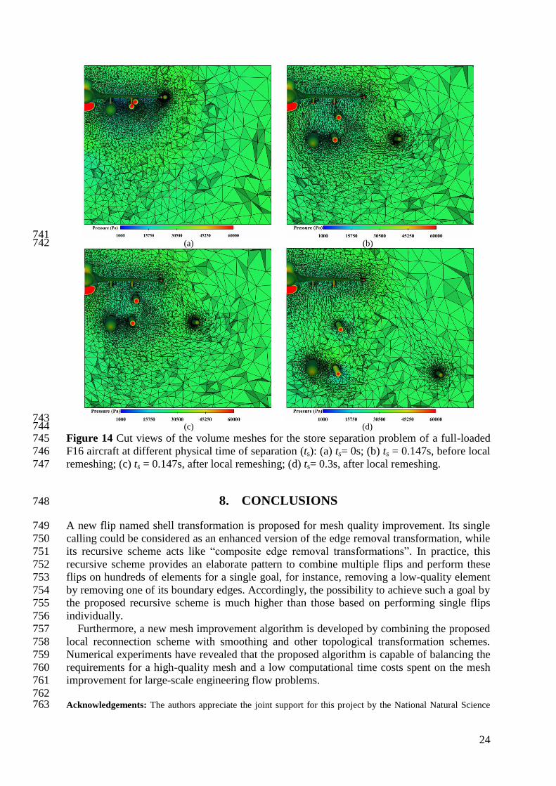
24

741 (a) (b) 742

743 (c) (d) 744

Figure 14 Cut views of the volume meshes for the store separation problem of a full-loaded 745

F16 aircraft at different physical time of separation (ts): (a) ts= 0s; (b) ts = 0.147s, before local 746

remeshing; (c) ts = 0.147s, after local remeshing; (d) ts= 0.3s, after local remeshing. 747

8. CONCLUSIONS 748

A new flip named shell transformation is proposed for mesh quality improvement. Its single 749

calling could be considered as an enhanced version of the edge removal transformation, while 750

its recursive scheme acts like “composite edge removal transformations”. In practice, this 751

recursive scheme provides an elaborate pattern to combine multiple flips and perform these 752

flips on hundreds of elements for a single goal, for instance, removing a low-quality element 753

by removing one of its boundary edges. Accordingly, the possibility to achieve such a goal by 754

the proposed recursive scheme is much higher than those based on performing single flips 755

individually. 756

Furthermore, a new mesh improvement algorithm is developed by combining the proposed 757

local reconnection scheme with smoothing and other topological transformation schemes. 758

Numerical experiments have revealed that the proposed algorithm is capable of balancing the 759

requirements for a high-quality mesh and a low computational time costs spent on the mesh 760

improvement for large-scale engineering flow problems. 761

762 Acknowledgements: The authors appreciate the joint support for this project by the National Natural Science 763

25

Foundation of China (Grant No. 11172267, 11432013, 10872182) and Zhejiang Provincial Natural Science 764 Foundation (Grant No. LR16F020002 and Y1110038). The first author acknowledges the joint support from 765 Zhejiang University and China Scholarship Council and the host of Professor Oubay Hassan and Professor 766 Kenneth Morgan for his recent research visit to Swansea University, UK. 767 768 REFERENCES 769

[1] Weatherill NP, Hassan O. Efficient three-dimensional Delaunay triangulation with automatic point creation 770 and imposed boundary constraints. Int. J. Numer. Methods Eng. 1994; 37:2005-2039. 771

[2] George PL, Borouchaki H, Saltel E. 'Ultimate' robustness in meshing an arbitrary polyhedron. Int. J. 772 Numer. Methods Eng. 2003; 58:1061-1089. 773

[3] Du Q, Wang D. Constrained boundary recovery for three dimensional Delaunay triangulations. Int. J. 774 Numer. Methods Eng. 2004; 61:1471-1500. 775

[4] Chen J, Zhao D, Huang Z, Zheng Y, Gao S. Three-dimensional constrained boundary recovery with an 776 enhanced Steiner point suppression procedure. Comput. Struct. 2011; 89:455-466. 777

[5] Si H. TetGen, a Delaunay-based quality tetrahedral mesh generator. ACM Trans. Math. Software 2015; 778 41:11:1-11:36. 779

[6] Joe B. Construction of three-dimensional improved-quality triangulations using local transformations. 780 SIAM J. Sci. Comput. 1995; 16:1292-1307. 781

[7] De L'Isle EB, George PL. Optimization of tetrahedral meshes. IMA Vol. Math. Appl. 1995; 75:97-128. 782 [8] de Cougny HL, Shephard MS. Refinement, derefinement, and optimization of tetrahedral geometric 783

triangulations in three dimensions.1995. Unpublished manuscript. 784 [9] Misztal M, Bærentzen J, Anton F, Erleben K. Tetrahedral mesh improvement using multi-face 785

retriangulation. Proceedings of the 18th International Meshing Roundtable, Salt Lake City, UT, USA, 786 2009; 539-555. 787

[10] Shewchuk JR. Two discrete optimization algorithms for the topological improvement of tetrahedral 788 meshes. 2002. Unpublished manuscript. April-15-2016. URL: https://www.cs.berkeley.edu/~jrs/papers/ 789 edge.pdf . 790

[11] Klingner BM, Shewchuk JR. Aggressive tetrahedral mesh improvement. Proceedings of the 16th 791 International Meshing Roundtable, Seattle, WA, USA, 2007; 3-23. 792

[12] Klingner BM, Shewchuk JR. Stellar: a tetrahedral mesh improvement program. Jan-21-2016. URL: 793 http://www.cs.berkeley.edu/~jrs/stellar. 794

[13] Klincsek GT. Minimal triangulations of polygonal domains. Ann. of Discrete Math. 1980; 9:121–123, 795 [14] Lo SH. 3D Delaunay triangulation of 1 billion points on a PC. Finite Elem. Anal. Des. 2015. 102-103: 65-796

73. 797 [15] Chen J, Zhao D, Huang Z, Zheng Y, Wang D. Improvements in the reliability and element quality of 798

parallel tetrahedral mesh generation. Int. J. Numer. Methods Eng. 2012; 92:671-693. 799 [16] Zhao D, Chen J, Zheng Y, Huang Z, Zheng J. Fine-grained parallel algorithm for unstructured surface mesh 800

generation. Comput. Struct. 2015; 154:177-191. 801 [17] Löhner R. Recent advances in parallel advancing front grid generation. Arch. Computat. Methods Eng. 802

2014; 21:127-140 803 [18] Joe B. Construction of three-dimensional Delaunay triangulations using local transformations. Comput. 804

Aided Geom. Des. 1991; 8:123-142. 805 [19] Compère G, Remacle JF, Jansson J, Hoffman J. A mesh adaptation framework for dealing with large 806

deforming meshes. Int. J. Numer. Methods Eng. 2010; 82:843-867. 807 [20] Freitag LA, Ollivier-Gooch C. Tetrahedral mesh improvement using swapping and smoothing. Int. J. 808

Numer. Methods Eng. 1997; 40:3979-4002. 809 [21] Liu J, Chen B, Sun S. Small polyhedron reconnection for mesh improvement and its implementation based 810

on advancing front technique. Int. J. Numer. Methods Eng. 2009; 79:1004 -1018. 811 [22] Field DA. Laplacian smoothing and Delaunay triangulations. Commun. Appl. Numer. Methods 1988; 812

4:709–712. 813 [23] Freitag LA, Knupp PM. Tetrahedral mesh improvement via optimization of the element condition number. 814

Int. J. Numer. Methods Eng. 2002; 53:1377-1391. 815 [24] Jiao X, Wang D, Zha H. Simple and effective variational optimization of surface and volume triangulations. 816

Eng. Comput. 2011; 27:81-94. 817 [25] Leng J, Zhang Y, Xu G. A novel geometric flow approach for quality improvement of multi-component 818

tetrahedral meshes. Comput.-Aided Des. 2013; 45:1182-1197. 819 [26] Vartziotis D, Wipper J. Fast smoothing of mixed volume meshes based on the effective geometric element 820

transformation method. Comput. Methods Appl. Mech. Eng. 2012; 201-204:65-81. 821 [27] Vartziotis D, Wipper J, Papadrakakis M. Improving mesh quality and finite element solution accuracy by 822

26

GETMe smoothing in solving the Poisson equation. Finite Elem. Anal. Des. 2013. 66: 36-52. 823 [28] Freitag DL, Knupp P, Munson T, Shontz S. A comparison of two optimization methods for mesh quality 824

improvement. Eng. Comput. 2006; 22:61-74. 825 [29] Cheng S-W, Dey TK, Shewchuk JR. Delaunay Mesh Generation. CRC Press, Boca Raton, Florida, 826

December 2012. 827 [30] Bedregal C, Rivara MC. Longest-edge algorithms for size-optimal refinement of triangulations. Comput.-828

Aided Des. 2014; 46:246–251. 829 [31] Ruppert J, Seidel R. On the difficulty of triangulating three-dimensional non-convex polyhedra. Discrete 830

Comput. Geom. 1992; 7:227-254. 831 [32] Ollivier-Gooch C. GRUMMP. April-15-2016. URL: http://tetra.mech.ubc.ca/GRUMMP. 832 [33] Model name: IRCADb patient-organs02 (model ID: 1477-IRCADb_patient-organs02). April-15-2016. 833

URL: http://visionair.ge.imati.cnr.it:8080/ontologies/shapes/view.jsp?id=1477-IRCADb_patient-organs02. 834 [34] Guimarães GF. F-16 Fighting Falcon. April-15-2016. URL: https://grabcad.com/library/f-16-fighting-835

falcon. 836 [35] Zheng J, Chen J, Zheng Y, Yao Y, Li S, Xiao Z. An improved local remeshing algorithm for moving 837

boundary simulations. Eng. Appl. Comp. Fluid 2016. 10: 405-428. 838