CHEMISTRY SEMESTER ONE - nglc [licensed for non...

CHEMISTRY SEMESTER ONE

SPECTROSCOPY LAB

Creative Commons Attribution 3.0 United States License 1

BEER-LAMBERT LAW

Lab format: this lab is a remote lab activity

Relationship to theory: This activity quantitatively relates the concentration of a light-

absorbing substance to the absorbance of light.

LEARNING OBJECTIVES

Read and understand these instructions BEFORE starting the actual lab procedure and

collecting data. Feel free to “play around” a little bit and explore the capabilities of the

equipment before you start the actual procedure (begins on page 13).

Measure and analyze the visible light absorbance spectrum of a standard NiSO4 solution

to determine the maximum wavelength of absorbance (λmax).

Measure the absorbance of several standard NiSO4 solutions.

Create Tables to display observations.

Construct a standard curve for the standard solutions. Find the relationship between

absorbance and concentration for NiSO4.

Measure the absorbance of an unknown concentration of the NiSO4 solution.

Calculate the concentration of the unknown NiSO4 solution using the standard curve

that you derived.

BACKGROUND INFORMATION

The energy of a photon of electromagnetic radiation is given by the relationship: E = hν where E = energy in joules, ν = frequency in cycles per second, and h = Planck’s constant = 6.63 x 10

-34 J/s

The relationship between wavelength and frequency of electromagnetic radiation is: λν= c

where λ = wavelength in meter and c = 2.996 x 108

m/s, the speed of radiant energy in a vacuum

Visible light represents only a very small part of the electromagnetic spectrum. Visible light consists of light having wavelengths from about 3.8 x 10-7m to 7.8 x 10-7 m (380 nm to 780 nm).

Many substances interact with electromagnetic radiation in the visible and ultraviolet regions of the spectrum. Substances that have color absorb some wavelengths from the visible region of the spectrum and reflect others. The energies associated with photons of visible and ultraviolet


SPECTROSCOPY LAB


light are in the same range as energies required to promote outer level (valence shell) electrons to higher energy level in many substances.

E = hλ is the difference in energy between the ground state and the excited state. When light of the appropriate wavelength impinges on a substance, it may be absorbed by promoting an electron to a higher energy level. This happens in the visible and ultraviolet regions of the spectrum.

In making measurements on the amount of radiant energy absorbed or transmitted by a sample, we use a blank so that the change in absorbance of the sample holder and the solvent can be factored out. That is, a blank containing all substances that will be in the sample, except the one under investigation, is placed in the spectrophotometer, and a measurement is taken so that we know how much light is absorbed by everything except the substance we are trying to investigate.

The absorbance of a solution can be related to the concentration of the absorbing species in the solution. This relationship is called the Beer-Lambert law, after Augustus Beer (a German physicist) and Johann Lambert (a Swiss physicist), but is commonly referred to as Beer’s Law. The Beer-Lambert Law can be expressed by:

A = abc

where A = Absorbance (unitless); a = molar absorptivity (molarity-1

∙cm-1

), which is a constant for the absorbing species, b = path length, or thickness of the absorbing layer of a solution (cm), and c = concentration of the solution (molarity).

Beer’s law tells us that the absorbance of a particular species is directly proportional to the concentration of the absorbing species. The measurement of a blank, as described above, allows us to factor out the effect of the solvent, cell walls and cell length.

So A = abc, and if a and b are constant for any given species and cell length, we can see that the absorbance of a solution is directly proportional to the concentration of the absorbing species. Because the absorbance of a solution is easy to measure, this technique is frequently used to measure concentrations of unknown solutions, and this is what you will be doing in this experiment.

EQUIPMENT

Paper

Pencil/pen

Computer (access to remote laboratory)


SPECTROSCOPY LAB


PREPARING TO USE THE RWSL SPECTROMETER

Setting up your computer for use with the RWSL:

Ensure that your computer system is capable of interacting with the RWSL microscope. Currently RWSL

works only on the Microsoft Windows operating system (XP or later) and a relatively up-to-date

browser. To confirm that your system meets minimum requirements, visit this website:

http://at.ccconline.org/rwsl/installguide/ and follow the steps provided.

Scheduling time at the RWSL

Go to your online class website in D2L and open the RWSL Scheduler. Select the date and time you

would like to attend lab. Try to choose a classroom that already has students scheduled in it so you

have some lab partners to work with.

Before you connect to the RWSL spectrometer:

Open the Mumble software and connect to the Denver NANSLO server. This will establish contact with

the Laboratory Technicians in the lab so they can assist you if you have any trouble.

Connecting to the RWSL spectrometer

When it is time to attend your scheduled lab, go to your online class website in D2L and open the RWSL

Scheduler. There will be a link just above the calendar that allows you to access the lab. NOTE: This link

will not be available until the exact time that your lab activity starts.

Figure 1 - RWSL Scheduler Link to Lab

http://at.ccconline.org/rwsl/installguide/


SPECTROSCOPY LAB


INTRODUCTION TO THE REMOTE EQUIPMENT AND INTERFACE:

DO NOT BEGIN WORKING ON THE LAB PROCEDURE UNTIL YOU HAVE READ ALL OF THIS INTRODUCTORY SECTION. THE PROCEDURE BEGINS ON PAGE 13. When you access the RWSL through the course website, you will see an interface that looks like this:

Figure 2 - RWSL Interface The controls on the right side of the screen are for controlling the camera. The preset positions allow you to quickly zoom in to a different part of the setup, but you can also pan, tilt and zoom the camera using the keypad controls on the screen. On the left side of the screen, you can see the controls for one of the pieces of equipment that is used in this experiment. It is called a Qpod, and it is a device into which a cuvette containing sample is placed so that light can be shined through it in order to measure absorbance. All of our cuvettes have a path length (distance that the light travels through them) of 1.00 cm.

Here is a cuvette: (photo from http://cuvette.net/ , really, that’s the name of the site) The Qpod is also capable of controlling the temperature of the sample inside of it. For clarity, here is a labeled picture of the equipment:

http://cuvette.net/


SPECTROSCOPY LAB


Figure 3 - Equipment for this lab The light path is also indicated with yellow arrows. Some of the fiber optic cabling that the light flows through is not visible in the photo, but you probably get the idea. The light is produced by a Xenon strobe inside the spectrometer, and then passed through a fiber optic cable into one side of the Qpod. The light passes through whatever sample is inside the Qpod, and then enters a fiber optic cable on the other side of the Qpod and is returned to the sensing unit in the spectrometer. Controlling the Qpod:

The first thing to do is to turn on the Qpod’s temperature control system and ensure that it is set to 25.00 °C, which is the standard temperature for most Absorbance measurements. You do this by gaining control of the interface and clicking the buttons labeled “Temperature Controller” and “Get QPod Temperature” (see Figure 4). Watch the temperature curve for a few minutes to ensure that the temperature of the Qpod is adjusted to 25.00 °C +/- 0.05 °C. There is also a tab for “Ramping Controls”, but they will not be used for this experiment, so you can ignore them.

QPod. The cuvette goes into a hole that is under the silver cap.

Spectrometer

Cuvettes in a rack Bucket of water that allows the Qpod to control the cuvette temperature


SPECTROSCOPY LAB


Figure 4 - Temperature Controls Basic Functions of the Spectrometer:

After the temperature of the Qpod has been set properly, you are ready to proceed with taking Absorbance measurements. Click the “Spectrometer” tab to proceed. The first thing to do is to take a “dark spectrum”, which is merely a measurement of what the spectrometer is measuring when there is no light present. This establishes a level of baseline “noise” in the instrument, which will be automatically subtracted out later in the process. First, on the Spectrometer tab of the interface, click the green button labeled “Start”. This enables the spectrometer to operate, and will change the button to a yellow “Pause” button. You take and store the dark spectrum by ensuring that the “Light” is not on, and then clicking the “Store Dark” button. There will be no indication that anything happened, so if you’re not sure you clicked this button, just click it again – you won’t hurt anything by storing another dark spectrum (see Figure 5).


SPECTROSCOPY LAB


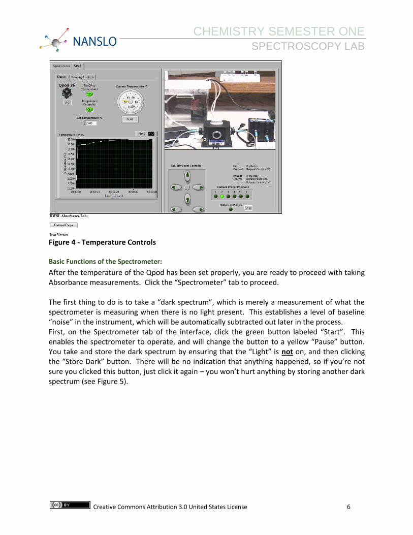
Figure 5 - Storing a Dark Spectrum At this point, turn on the spectrometer’s light source by clicking the “Light” button, which will then turn green. You should now see a spectrum on the screen that looks like this (Figure 6):

Click Here to store Dark spectrum


SPECTROSCOPY LAB


Figure 6 - Light Spectrum Now you need to collect and store the spectrum of the “reference sample”. The reference sample is just a cuvette full of distilled water. Putting this cuvette into the Qpod and clicking the “Store Ref” button will store a spectrum where light is being absorbed by the cuvette and by water. Having this spectrum stored allows it to be subtracted out from your later sample measurements, thus allowing you to measure the Absorption of light that is only due to the material you are interested in (NiSO4 in this experiment).


SPECTROSCOPY LAB


Figure 7 - Storing the Reference Spectrum Now you are ready to measure the absorbance of nickel (II) sulfate. There are several standard NiSO4 solutions that you will measure the absorbance of. This range of concentrations was chosen because the Absorbance is directly proportional to the concentration (Obeys Beer’s law) in this concentration range. By plotting Absorbance on the y-axis and concentration of NiSO4 on the x-axis, you will draw a best-fit straight line (which is called the “standard curve”) passing through the origin. When you measure the absorbance of the sample, you must do so at a single wavelength. This is called the λmax, and corresponds to the tallest peak in the absorbance spectrum. It is important that this wavelength be the one at which the sample absorbs light the most strongly because this results in the most favorable signal-to-noise ratio and gives an absorbance measurement with the least amount of uncertainty. Zooming in and out on the Spectrum:

With a cuvette containing NiSO4 solution in the Qpod, make sure the light is on and that the spectrum graph is zoomed all the way out. Here are the steps for doing this:

a. Click on the button at the lower right of the graph, shown below in Figure 8.

b. This brings up a small sub-menu of other buttons. The only two that are useful

to you are the left-most buttons in the top and bottom rows (See Figure 9),

Click Here to store Reference Spectrum


SPECTROSCOPY LAB


although you can play around with the others if you want to. Select the left-

most button in the bottom row to view the entire spectrum.

c. Select the left-most in the top row to select specific parts of the spectrum to

“zoom in” on and view more closely. After clicking this button, you use the

mouse to draw a box around the area that you want to zoom in to. Be sure you

draw the box so that it includes some area past the top of the peak you are

interested in, or else it will chop off the top of it in the viewing window.

d. If you accidentally zoom in too far or on the wrong part of the spectrum, just

zoom out and start over again.

Finding λmax:

This is merely identifying the tallest peak in the spectrum, and you only need to do this once for a chemical, no matter how many different solution concentrations you measure. With a cuvette containing NiSO4 solution in the Qpod, and the light turned on, and the cursor enabled, click the “Show Absorbance Spectrum” button and then zoom all the way out on the spectrum. You will now see the absorbance spectrum of the sample, as in Figure 10. Click the Cursor Control button and move the cursor on top of the tallest peak using the mouse.

Figure 8 – Spectrum Manipulation Button

Figure 9 - These two buttons are most useful

Zoom In

Zoom Out


SPECTROSCOPY LAB


Figure 10 - Absorbance Spectrum You can ignore the noisy parts of the spectrum on either end. There may be one peak as shown below, or there may be more than one. Always use the tallest absorbance peak. Now, you can read the wavelength of the tallest peak on the “Cursor Location Information” line. In this case, the tallest peak is at 393.4 nm. This is λmax, and the absorbance at λmax is shown in the Absorbance at Wavelength box. Remember, λmax does not change as long as you are measuring the absorbance of the same chemical (NiSO4 in this experiment), so you do not need to adjust the cursor location after you have it set.

Enable Cursor button

Cursor Control button

Absorbance button

Absorbance Value at cursor location


SPECTROSCOPY LAB


Smoothing out the Absorbance spectrum:

Do you notice how much the Absorbance reading is jumping around? This is due to noise in the data. Look back at the Spectrometer Tab (Figure 11). See the fields called “Integration Time”, “Boxcar Width” and “# Spectra to Average”? These are variables that you can adjust to “clean up” the noise in the spectrum. For now, let’s just use the “# Spectra to Average” variable. The spectrometer collects a spectrum about once every 100 milliseconds. The “Average” variable tells the spectrometer how many spectra to average before it reports a result. Just like any other measurement that contains random error (“noise”), averaging several measurements can average out the noise and “clean up” the signal. Try setting the “# Spectra to Average” field to some numbers between 1 and 50 and see what the result is on the Absorbance measurement for a sample. Once you find a setting that gives you results that you think are good, stick with it.

Figure 11 - Variables on the Spectrometer Tab


SPECTROSCOPY LAB


EXPERIMENTAL PROCEDURE:

(REFERENCE THE ABOVE SECTIONS FOR DETAILS)

1. Log into Mumble and establish communication with the Lab Technician.

2. Using the link in the RWSL Scheduler on your course webpage, access the RWSL and

take control of the interface.

3. Request that the Lab Tech ensure that there is no cuvette in the spectrometer. Ensure

the Light is turned off. Collect a Dark spectrum.

4. Request that the Lab Tech insert the Reference Sample into the spectrometer. Collect

the Reference spectrum.

5. Ask the Lab Tech what the solution concentrations are for the standard NiSO4 solutions.

6. Request that the Lab Tech insert a NiSO4 cuvette into the spectrometer. Determine the

location of λmax.

7. View the Absorbance Spectrum.

8. Record the Absorbance of the NiSO4 sample at λmax. Each student in the group must

write the measurement down for later use.

9. Ask the lab Tech to insert the cuvette with the next higher concentration of NiSO4 into

the spectrometer.

10. Repeat steps 8 and 9 for all remaining samples, including the cuvette with the unknown

concentration of NiSO4.

11. Another student should take control of the interface and repeat the process starting at

step 2.

12. After each student has collected a complete set of data (and everyone has recorded

each data set), you can log out of the lab and work on the data analysis portion. If you

have time left in your scheduled lab period, you can continue working with your lab

partners in Mumble to analyze the data.

Data Analysis:

Plot a standard graph using the concentration and Absorbance values for the standard solutions. Plot Concentration on the X-axis and Absorbance values on the Y-axis. Draw a best-fit line going through the origin. From the Absorbance of the unknown solution, you can calculate the concentration of the unknown solution using the line equation of the standard curve. In Excel, the best-fit line and its equation can be determined by this method:

a. Insert a scatter plot of the data, making sure that absorbance is on the y axis and

concentration is on the x axis. If they are switched, then delete the graph, change the

positions of the absorbance and concentration columns and insert the scatter plot graph

again.


SPECTROSCOPY LAB


b. Right-click one of the data points on the graph and select Add Trendline.

c. Make sure “Linear” is selected and check the box to set the intercept to zero and also

the one to display the equation on the chart.

d. You will now have the best-fit line and the equation for that line. You can use this line

equation to calculate the concentration of the unknown NiSO4 solution.

Write a lab report using the same format that you use for all your other CHE111 reports. Be sure and show all applicable graphs and equations for calculating the concentration of NiSO4 in the unknown sample. Make sure that all the objectives of this Lab are addressed in your report. Answer the following questions at the end of your report:

A. Why do you have to first take an absorbance measurement of a cuvette filled with

distilled water? Why does this measurement have to be subtracted from the

measurements of the NiSO4 samples?

B. Why didn’t we just measure one or two samples with known concentrations of NiSO4?

C. How many significant digits can you report in the concentration of the unknown

sample? What limits the number of significant digits in this result?

D. What is the energy, in Joules, of one photon of light at λmax?

E. What color is the NiSO4 solution? What color is the light that is being absorbed at λmax?

Here’s some information that may help you in this quest. What pattern do you notice

here? (Hint: find a “color wheel” and compare it to this chart)

Observed Color of Solution

Approximate wavelength of reflected light (nm)

Color of light that is being absorbed by solution

Approximate wavelength of light being absorbed (nm)

Greenish-yellow 560 Violet 400 nm

Yellow 600 Blue 450

Red 620 Blueish-green 490

Violet 410 Yellowish-green 570

Blue-violet 430 Yellow 580

Blue 450 Orange 600

Green 520 Red 650

F. If a chemical solution was primarily yellow in color, what color would you expect λmax of

the absorbed light to be? Why?

G. Do some research and find one useful application of Beer’s Law in the chemical industry,

environmental analysis or some other applied field of chemistry.

CHEMISTRY SEMESTER ONE - nglc [licensed for non...

Documents

Transcript of CHEMISTRY SEMESTER ONE - nglc [licensed for non...