1

Chemical Reaction Dynamics

David E. Manolopoulos

Contents

I. Introduction 2

II. Quantum Scattering Theory 2

A. Free particle eigenstates 2

B. Scattering eigenstates 5

C. Flux and unitarity 7

D. The scattering Green’s function 9

E. Formal scattering theory 12

III. Chemical Reaction Rate Theory 15

A. The thermal rate coefficient 15

B. Miller’s trace formula 16

C. A simpler projection operator 17

D. Side-side, flux-side and flux-flux correlation functions 20

IV. The Classical Limit 22

A. Classical partition functions 22

B. Classical correlation functions 23

C. Classical transition state theory 25

D. Quantum transition state theory? 27

V. Further Reading 29

VI. Appendices 30

A. The Dirac delta function 30

B. The Heisenberg picture 32

C. Liouville’s theorem 33

2

I. INTRODUCTION

In these lectures, I will present an introduction to quantum scattering theory and to

the quantum theory of chemical reaction rates, at a level that will hopefully be accessible

to students with a good working knowledge of bound state quantum mechanics but little

or no previous knowledge of continuum wave functions. In order to do this in four lec-

tures, I will present the entire theory in the context of a simple one dimensional barrier

transmission problem, and leave to further reading how the final result (Miller’s flux-side

correlation function expression for the reaction rate coefficient1,2) can be applied to more

general reactions.

II. QUANTUM SCATTERING THEORY

A. Free particle eigenstates

The simplest possible continuum wave functions are the eigenstates of the free particle

Hamiltonian

H0 =p2

2m. (1)

Since H0 commutes with p, its eigenstates can be chosen to be eigenstates of the momentum

operator. Calling these eigenstates |p〉 and the momentum eigenvalues p, one has both

H0 |p〉 = E |p〉 (2)

and

p |p〉 = p |p〉 , (3)

with E = p2/2m.

It is straightforward to find the form of the momentum eigenstates in the position repre-

sentation, where

p = −ih ddx

(4)

and

〈x|p〉 = φp(x) (5)

convert Eq. (3) into a first order differential equation

−ih ddxφp(x) = p φp(x), (6)

3

the solution of which is

φp(x) ≡ 〈x|p〉 = Ne+ipx/h. (7)

Note that this also gives the form of the position eigenstates in the momentum representa-

tion,

φp(x)∗ ≡ 〈p|x〉 = N∗e−ipx/h. (8)

The normalization of the momentum eigenstates is a little tricky, because the normal-

ization integral 〈p|p〉 is undefined. (In other words, the momentum eigenstate |p〉 is not

a “proper” state vector in the space of square integrable functions in one dimension, and

neither for that matter is the position eigenstate |x〉. Both are nevertheless extremely useful

in quantum scattering theory as we are about to see.) The only way to make any sense

of the situation is to recognize that the overlap integral between two different momentum

eigenstates,

〈p′|p〉 =∫ ∞−∞

dx φp′(x)∗φp(x)

=∫ ∞−∞

dx 〈p′|x〉 〈x|p〉

= |N |2∫ ∞−∞

dx e−i(p′−p)x/h, (9)

is proportional to a Dirac delta function (see Appendix A)

δ(p′ − p) =1

2πh

∫ ∞−∞

dx e−i(p′−p)x/h. (10)

This suggests choosing N = (2πh)−1/2 in Eqs. (7) and (8), so that3

〈x|p〉 = (2πh)−1/2e+ipx/h (11)

and

〈p|x〉 = (2πh)−1/2e−ipx/h (12)

giving

〈p′|p〉 = δ(p′ − p). (13)

The momentum eigenstates form a complete set of states because they are the only

eigenstates of the free particle Hamiltonian H0 (which does not support any bound states).

This means that any state |ψ〉 of a one-dimensional system can be expanded in terms of the

momentum eigenstates as

|ψ〉 =∫ ∞−∞

dp |p〉 〈p|ψ〉 . (14)

4

In the position representation this reads

〈x|ψ〉 =∫ ∞−∞

dp 〈x|p〉 〈p|ψ〉 , (15)

or equivalently

ψ(x) =1

(2πh)1/2

∫ ∞−∞

dp e+ipx/hψ(p). (16)

Applying the Fourier inversion theorem to this gives

ψ(p) =1

(2πh)1/2

∫ ∞−∞

dx e−ipx/hψ(x), (17)

or equivalently

〈p|ψ〉 =∫ ∞−∞

dx 〈p|x〉 〈x|ψ〉 , (18)

and taking this out of the momentum representation leaves

|ψ〉 =∫ ∞−∞

dx |x〉 〈x|ψ〉 . (19)

Thus the position eigenstates also form a complete set of states, and indeed setting |ψ〉 = |x′〉

in Eq. (15) gives

〈x|x′〉 =∫ ∞−∞

dp 〈x|p〉 〈p|x′〉

=1

(2πh)

∫ ∞−∞

dp e−ip(x′−x)/h

= δ(x′ − x). (20)

Equations (13), (14), (19) and (20) are the main results so far. They show that the

momentum eigenstates |p〉 and the position eigenstates |x〉 each form a complete set of

orthonormal states. These results are entirely analogous to those obtained in a discrete

basis of “proper” square integrable state vectors such as the eigenstates |n〉 of a harmonic

oscillator, in which one has the more familiar orthonormality condition

〈n′|n〉 = δn′n (21)

and the completeness relation

|ψ〉 =∞∑n=0

|n〉 〈n|ψ〉 , (22)

The only differences that arise in the momentum and position eigenstate bases are that

the Kronecker delta in Eq. (21) becomes a Dirac delta function and the sum over states in

Eq. (22) becomes an integral.

5

One other thing we shall need to know how to do is calculate the trace of an operator in

these two bases. In a basis set of harmonic oscillator eigenstates, the trace of an operator A

is

tr[A]

=∞∑n=0

⟨n|A|n

⟩, (23)

and this is independent of the force constant that is chosen for the harmonic oscillator

because the transformation between any one (complete, orthonormal) basis and any other

is a unitary transformation. In the momentum and position eigenstate bases, one can write

either

tr[A]

=∫ ∞−∞

dp⟨p|A|p

⟩, (24)

or

tr[A]

=∫ ∞−∞

dx⟨x|A|x

⟩, (25)

both of which will again give the same result as can be seen from the following argument:

∫ ∞−∞

dp⟨p|A|p

⟩=∫ ∞−∞

dp∫ ∞−∞

dx∫ ∞−∞

dx′ 〈p|x〉⟨x|A|x′

⟩〈x′|p〉

=1

2πh

∫ ∞−∞

dp∫ ∞−∞

dx∫ ∞−∞

dx′ e−ip(x−x′)/h

⟨x|A|x′

⟩=∫ ∞−∞

dx∫ ∞−∞

dx′ δ(x− x′)⟨x|A|x′

⟩=∫ ∞−∞

dx⟨x|A|x

⟩. (26)

Exercise 1. Any operator A that acts on the space of square integrable functions in one

dimension can be written in terms of the eigenstates |n〉 of a harmonic oscillator as

A =∞∑n=0

∞∑n′=0

|n〉⟨n|A|n′

⟩〈n′| . (27)

(a) Why is this? (b) Use this expression to show that Eq. (25) will give the same result as

Eq. (23) for tr[A].

B. Scattering eigenstates

Now consider a more general problem with a Hamiltonian of the form

H = H0 + V =p2

2m+ V (x), (28)

6

x

V(x)

E

ψp(x) ~ φ

p(x) + φ−p

(x) R(E) ψp(x) ~ φ

p(x) T(E)

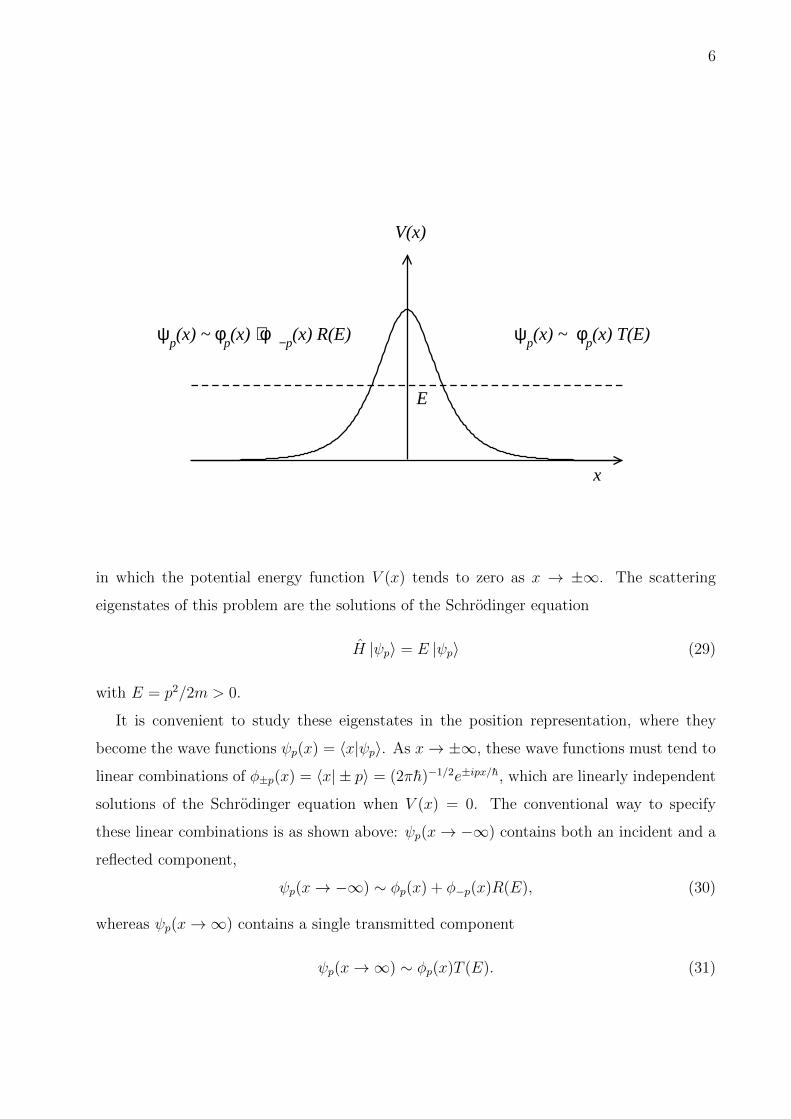
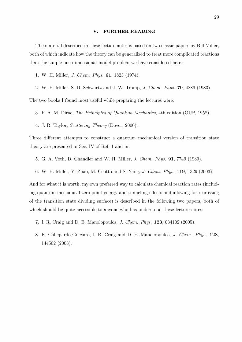
in which the potential energy function V (x) tends to zero as x → ±∞. The scattering

eigenstates of this problem are the solutions of the Schrodinger equation

H |ψp〉 = E |ψp〉 (29)

with E = p2/2m > 0.

It is convenient to study these eigenstates in the position representation, where they

become the wave functions ψp(x) = 〈x|ψp〉. As x→ ±∞, these wave functions must tend to

linear combinations of φ±p(x) = 〈x| ± p〉 = (2πh)−1/2e±ipx/h, which are linearly independent

solutions of the Schrodinger equation when V (x) = 0. The conventional way to specify

these linear combinations is as shown above: ψp(x→ −∞) contains both an incident and a

reflected component,

ψp(x→ −∞) ∼ φp(x) + φ−p(x)R(E), (30)

whereas ψp(x→∞) contains a single transmitted component

ψp(x→∞) ∼ φp(x)T (E). (31)

7

The reflection amplitude R(E) and the transmission amplitude T (E) can be obtained for any

potential V (x) by solving the Schrodinger equation in the interaction region. For example,

in the trivial case where the potential is zero, the only solution of the Schrodinger equation

that is compatible with both boundary conditions is ψp(x) = φp(x), giving R(E) = 0 and

T (E) = 1.

Exercise 2. Consider the scattering from the potential energy barrier

V (x) =

0, x < 0

V0, 0 < x < a

0, x > a

(32)

in which V0 > 0. Use the fact that ψp(x) and ψ′p(x) must both be continuous at x = 0 and

x = a to obtain explicit expressions for the reflection amplitude R(E) and the transmission

amplitude T (E) when E = V0, and verify that your expressions satisfy

|R(E)|2 + |T (E)|2 = 1. (33)

C. Flux and unitarity

Equation (33) shows that the reflection and transmission probabilities for the problem

considered in exercise 2 sum to one (“unitarity”). This is a general result that can be shown

to hold for any potential V (x) and any scattering energy E as follows.

The flux (number of particles per unit time) passing through the point x = s is given in

quantum mechanics by the Heisenberg time derivative of the projection operator onto the

subspace in which x > s, namely (see Appendix B)

F (s) =i

h

[H, h(x− s)

], (34)

where

h(x− s) =

1, if x > s

0, if x < s. (35)

For a Hamiltonian of the form in Eq. (28), it is straightforward (and therefore left as an

exercise) to show that F (s) can be written in the position representation as

F (s) = − ih

2m

δ(x− s) d

dx+

d

dxδ(x− s)

. (36)

8

The flux through s for a general time-dependent wave function ψ(x, t) is therefore

j(s, t) ≡ 〈ψ| F (s) |ψ〉 = − ih

2m

ψ(s, t)∗

∂ψ(s, t)

∂s− ∂ψ(s, t)

∂s

∗

ψ(s, t)

, (37)

and it is equally straightforward to show (another exercise) that this satisfies the quantum

mechanical continuity equation

∂

∂sj(s, t) = − ∂

∂t|ψ(s, t)|2. (38)

The most important implication of these equations is that the flux j(s, t) will be a con-

stant (independent of both s and t) when ψ(s, t) = ψ(s, 0)e−iEt/h is an eigenstate of the

Hamiltonian (a stationary state). If this stationary state is a bound state its wave function

ψ(s, 0) may be chosen to be real, and it follows from this that j(s, t) will be identically

zero for all s and t. So bound states do not contribute any flux, but scattering states do:

inserting the scattering eigenstate |ψp〉 into Eq. (37), and choosing s to be in the asymptotic

“product” region where the boundary condition in Eq. (31) applies, we obtain

〈ψp| F (s) |ψp〉 = 〈p| F (s) |p〉 |T (E)|2

= − ih

2m

φp(s)

∗ d

dsφp(s)− φp(s)

d

dsφp(s)

∗|T (E)|2

= − ih

2m

1

2πh

e−ips/h

d

dse+ips/h − e+ips/h d

dse−ips/h

|T (E)|2

= − ih

2m

1

2πh

2ip

h|T (E)|2 =

1

2πh

(p

m

)|T (E)|2. (39)

Had we chosen instead to place s in the asymptotic “reactant” region where the boundary

condition in Eq. (30) applies, we would have obtained⟨ψp|F (s)|ψp

⟩=

1

2πh

(p

m

) (1− |R(E)|2

). (40)

And since the flux is independent of s for a stationary state, this completes the proof of

Eq. (33).

Exercise 3. (a) Use Eqs. (28) and (34) to derive the expression for the flux operator

in Eq. (36). (b) Derive the continuity equation in Eq. (38) from Eq. (37) and the time-

dependent Schrodinger equation in the form

∂

∂tψ(s, t) = − i

h

[− h2

2m

∂2

∂s2+ V (s)

]ψ(s, t).

(c) Verify the result in Eq. (40).

9

D. The scattering Green’s function

The full scattering Schrodinger equation is

H |ψp〉 =(H0 + V

)|ψp〉 = E |ψp〉 . (41)

Rearranging this gives

(E − H0) |ψp〉 = V |ψp〉 , (42)

which can be solved formally to give

|ψp〉 = |χp〉+ limε→0

(E + iε− H0)−1V |ψp〉 (43)

where |χp〉 satisfies the free particle Schrodinger equation

(E − H0) |χp〉 = 0. (44)

In the language of linear second order differential equations, the first term on the right-hand

side of Eq. (43) is a “complementary function” and the second is a “particular integral”; the

iε in this integral is a tiny embellishment that is needed to make the inverse of the operator

(E − H0) well defined (see exercise 4 below).

In the position representation, Eq. (43) becomes an integral equation for the scattering

wave function ψp(x) ≡ 〈x|ψp〉,

ψp(x) = χp(x) +∫ ∞−∞

dx′G+0 (x, x′)V (x′)ψp(x

′), (45)

where

G+0 (x, x′) = lim

ε→0〈x| (E + iε− H0)−1 |x′〉 . (46)

Letting pε =√

2m(E + iε), and noting that H0 = p2/2m, one can evaluate this free particle

Green’s function as follows:

G+0 (x, x′) = lim

ε→0〈x| (E + iε− H0)−1 |x′〉

= limε→0

∫ ∞−∞

dp′ 〈x| (E + iε− p2/2m)−1 |p′〉 〈p′|x′〉

= limε→0

∫ ∞−∞

dp′ 〈x|p′〉 (p2ε/2m− [p′]2/2m)−1 〈p′|x′〉

= limε→0

2m

2πh

∫ ∞−∞

dp′e+ip′(x−x′)/h

(p2ε − [p′]2)

= − limε→0

m

πh

∫ ∞−∞

dp′e+ip′(x−x′)/h

(p′ − pε)(p′ + pε). (47)

10

ε−p

+p

Re p’

Im p’

x−x’<0

x−x’>0

.

ε

For small positive ε, the poles in the integrand of Eq. (47) at p′ = ±pε = ±√

2m(E + iε)

are shifted off the real integration axis into the first and third quadrants of the complex

p′ plane (see above). The integral is therefore well defined and can be evaluated using the

residue theorem. When x > x′, the integration contour can be closed along a semicircle at

infinity in the upper half of the complex plane, enclosing the simple pole at p′ = +pε. The

semicircle does not make any contribution to the contour integral and the residue theorem

gives

G+0 (x, x′) = − lim

ε→0

m

πh2πiR(+pε) = − lim

ε→0

m

πh2πi

e+ipε(x−x′)/h

2pε

= − limε→0

im

hpεe+ipε(x−x′)/h = −im

hpe+ip(x−x′)/h (x > x′), (48)

where p = limε→0 pε =√

2mE. When x < x′, the contour can be closed along a semicircle

at infinity in the lower half of the complex plane (which again makes no contribution), and

the residue theorem gives

G+0 (x, x′) = + lim

ε→0

m

πh2πiR(−pε) = − lim

ε→0

m

πh2πi

e−ipε(x−x′)/h

2pε

= − limε→0

im

hpεe−ipε(x−x

′)/h = −imhpe−ip(x−x

′)/h (x < x′), (49)

where the initial sign change arises because the contour is now clockwise. So overall

G+0 (x, x′) = −im

hpe+ip|x−x′|/h = −2πim

pφ−p(x<)φp(x>), (50)

11

where φ±p(x) = (2πh)−1/2e±ipx/h and x< (x>) is the lesser (greater) of x and x′.

The final stage of the argument is to substitute this back into Eq. (45) and to use the

boundary conditions on ψp(x) in Eqs. (30) and (31) to determine the homogeneous solution

χp(x). As x→ −∞, Eqs. (45) and (50) give

ψp(x→ −∞) ∼ χp(x)− 2πim

pφ−p(x)

∫ ∞−∞

dx′ φp(x′)V (x′)ψp(x

′)

= χp(x)− 2πim

pφ−p(x)

∫ ∞−∞

dx′ φ−p(x′)∗V (x′)ψp(x

′). (51)

Comparing this with Eq. (30), and noting that the coefficients of φp(x) and φ−p(x) must be

the same in both equations, fixes

χp(x) = φp(x) (52)

and gives

R(E) = −2πim

p

⟨−p|V |ψp

⟩. (53)

Finally, as x→∞, Eqs. (45), (50) and (52) give

ψp(x→∞) ∼ φp(x)− 2πim

pφp(x)

∫ ∞−∞

dx′ φ−p(x′)V (x′)ψp(x

′)

= φp(x)− 2πim

pφp(x)

∫ ∞−∞

dx′ φp(x′)∗V (x′)ψp(x

′), (54)

and comparing this with Eq. (31) gives

T (E) = 1− 2πim

p

⟨p|V |ψp

⟩. (55)

Exercise 4. The need for the iε in Eq. (43) arises because the resolvent operator (z−H0)−1

has a branch cut along the positive real z axis, on which z = E is an eigenvalue of H0. Prove

this by showing that when the real axis is approached from below, as it is in

G−0 (x, x′) = limε→0〈x| (E − iε− H0)−1 |x′〉 , (56)

one obtains a result that differs from the one in Eq. (50). (The reason why we have chosen

to focus on G+0 (x, x′) here is that it is consistent with the boundary conditions on ψp(x)

in Eqs. (30) and (31), whereas G−0 (x, x′) is not; ψp(x) is sometimes called ψ+p (x) in the

literature for this reason.)

12

E. Formal scattering theory

The free particle Green’s function G+0 (x, x′) in Eq. (50) is a position matrix element of

the free particle Green’s operator

G+0 (E) = lim

ε→0

(E + iε− H0

)−1, (57)

and one can clearly define an analogous operator for the full scattering problem:

G+(E) = limε→0

(E + iε− H

)−1. (58)

These two operators are related by the fact that H = H0 + V , which implies that

G+0 (E)−1 = G+(E)−1 + V . (59)

Pre-multiplying Eq. (59) by G+(E) and post-multiplying by G+0 (E) gives

G+(E) = G+0 (E) + G+(E)V G+

0 (E), (60)

whereas pre-multiplying by G+0 (E) and post-multiplying by G+(E) gives

G+(E) = G+0 (E) + G+

0 (E)V G+(E). (61)

These two equations are known as the Lippmann-Schwinger equations4 for G+(E).

In view of Eqs. (43) and (52), the free particle Green’s operator G+0 (E) provides a link

between the scattering eigenstate |ψp〉 and the free particle (momentum) eigenstate |p〉:

|ψp〉 = |p〉+ G+0 (E)V |ψp〉 . (62)

This can be solved to give |ψp〉 explicitly as

|ψp〉 =[1− G+

0 (E)V]−1|p〉 . (63)

An alternative expression for |ψp〉 is obtained by noting that both

[1 + G+(E)V

] [1− G+

0 (E)V]

= 1, (64)

and [1− G+

0 (E)V] [

1 + G+(E)V]

= 1, (65)

13

where Eq. (64) follows from Eq. (60) and Eq. (65) from Eq. (61); therefore

[1− G+

0 (E)V]−1

=[1 + G+(E)V

](66)

and

|ψp〉 =[1 + G+(E)V

]|p〉 . (67)

Note in passing that this expression implies that Eq. (55) can be written more symmetrically

as

T (E) = 1− 2πim

p〈p| T (E) |p〉 (68)

where T (E) is the transition operator4

T (E) = V + V G+(E)V . (69)

Returning to Eq. (67), and recalling that V = H − H0 and H0 |p〉 = E |p〉, one finds that

the following formal manipulations1 give yet another expression for |ψp〉:

|ψp〉 =[1 + G+(E)V

]|p〉

=[1− G+(E)(E − H)

]|p〉

= limε→0

[1− (E + iε− H)−1(E − H)

]|p〉

= limε→0

[1− (E + iε− H)−1(E + iε− H − iε)

]|p〉

= limε→0

(iε)(E + iε− H)−1 |p〉

= limε→0

(iε)(ih)−1∫ ∞

0dt e+i(E+iε−H)t/h |p〉

= limε→0

ε

h

∫ ∞0

dt e−εt/he−iHt/he+iEt/h |p〉

= limε→0

ε

h

∫ ∞0

dt e−εt/he−iHt/he+iH0t/h |p〉

= limε→0

∫ ∞0

dx e−xe−iHx/εe+iH0x/ε |p〉

= limt→∞

∫ ∞0

dx e−xe−iHt/he+iH0t/h |p〉

= limt→∞

e−iHt/he+iH0t/h |p〉

= Ω+ |p〉 , (70)

where Ω+ is the Møller operator4

Ω+ = limt→∞

e−iHt/he+iH0t/h. (71)

14

The physical interpretation of this result is that the scattering eigenstate |ψp〉 can be obtained

by propagating the free-particle eigenstate |p〉 back into the infinite past under the influence

of the free-particle Hamiltonian H0, and then propagating the result forward to time t = 0

under the influence of the full Hamiltonian H.

An important implication of Eq. (70) is that the full scattering eigenstates are normalized

in the same way as the free particle eigenstates:

〈ψp′ |ψp〉 = 〈p′| Ω†+Ω+ |p〉

= limt→∞〈p′| e−iH0t/he+iHt/he−iHt/he+iH0t/h |p〉

= 〈p′|p〉 = δ(p′ − p). (72)

If the Hamiltonian H does not support any bound states, this implies by analogy with

Eqs. (14) and (24) that any state |ψ〉 can be expanded in terms of the scattering eigenstates

as

|ψ〉 =∫ ∞−∞

dp |ψp〉 〈ψp|ψ〉 , (73)

and that the trace of an operator A can be calculated as

tr[A]

=∫ ∞−∞

dp 〈ψp| A |ψp〉 . (74)

If H does support some bound states |ψb〉, such that H |ψb〉 = Eb |ψb〉 with 〈ψb′|ψb〉 = δb′b

and Eb′ , Eb < 0, these will be orthogonal to the scattering states as they are eigenstates of

the same Hermitian operator with different eigenvalues (recall that H |ψp〉 = E |ψp〉 with

E = p2/2m > 0). It follows from this that each of the above equations will simply be

augmented by a bound-state contribution:

|ψ〉 =∑b

|ψb〉 〈ψb|ψ〉+∫ ∞−∞

dp |ψp〉 〈ψp|ψ〉 , (75)

and

tr[A]

=∑b

〈ψb| A |ψb〉+∫ ∞−∞

dp 〈ψp| A |ψp〉 . (76)

Note finally that, according to the argument in Eq. (72), the operator Ω†+Ω+ behaves like

a unit operator when acting on any free particle eigenstate:

Ω†+Ω+ |p〉 = |p〉 . (77)

15

Since the free particle eigenstates are complete (H0 does not support any bound states), this

implies that Ω†+Ω+ is a unit operator:

Ω†+Ω+ = 1. (78)

If it were also true that Ω+Ω†+ = 1, then Ω+ would be unitary. However, this is not true

when the Hamiltonian H supports any bound states, as can be seen from the following

argument:

〈p| Ω†+ |ψb〉 = 〈ψb| Ω+ |p〉∗ = 〈ψb|ψp〉∗ = 0. (79)

Since this is true for all |p〉, and the free particle eigenstates are complete, it implies that

Ω+Ω†+ |ψb〉 = 0 (80)

for all bound states |ψb〉, and it is immediately apparent from this that

Ω+Ω†+ 6= 1 (81)

(in fact, Ω+Ω†+ is just a projection operator onto the subspace of scattering eigenstates,

as shown in exercise 5 below). An operator Ω+ that satisfies Eqs. (78) and (81) is norm-

preserving (or isometric), but it is not unitary.4

Exercise 5. Starting with Eq. (62) in the form |p〉 =[1− G+

0 (E)V]|ψp〉, and recalling that

V = H−H0 and H |ψp〉 = E |ψp〉, show by following the steps in Eq. (70) that |p〉 = Ω†+ |ψp〉

where Ω†+ = limt→∞ e−iH0t/he+iHt/h. This implies that Ω+Ω†+ |ψp〉 = Ω+ |p〉 = |ψp〉 for any

|ψp〉, which in conjunction with Eq. (80) shows that Ω+Ω†+ is a projection operator onto the

subspace of scattering eigenstates; a simpler way to see this is to note that

Ω+Ω†+ = Ω+1 Ω†+ =∫dp Ω+ |p〉 〈p| Ω† =

∫dp |ψp〉 〈ψp| .

III. CHEMICAL REACTION RATE THEORY

A. The thermal rate coefficient

The one-dimensional barrier transmission problem illustrated in the figure on page 6 is the

simplest possible model for a bimolecular chemical reaction, with the reactant asymptote at

16

x→ −∞ and the product asymptote at x→∞. The exact quantum mechanical expression

for the thermal rate coefficient of this “reaction” is

k(T ) =1

2πhQr(T )

∫ ∞0

dE e−βEN(E), (82)

where β = 1/(kBT ). Here Qr(T ) is the reactant partition function per unit length (it would

become the partition function per unit volume for a reaction in three-dimensional space),

which is given by elementary statistical mechanics as

Qr(T ) =1

Λ(T )=

(2πmkBT

h2

)1/2

=

(m

2πβh2

)1/2

, (83)

and N(E) is the “cumulative reaction probability”,2 which in the present case of a one-

dimensional barrier transmission problem is simply the barrier transmission probability

N(E) = |T (E)|2 . (84)

Exercise 6. Verify that k(T ) in Eq. (82) has the correct dimensions for a bimolecular (sec-

ond order) rate coefficient in one-dimensional space, where “concentrations” are measured

in terms of the number of particles per unit length.

B. Miller’s trace formula

The flux-side correlation function formulation of Miller and co-workers1,2 provides an

extremely elegant (and entirely rigorous) way to calculate the rate coefficient in Eq. (82),

and one that has a clear connection with the classical limit (and classical transition state

theory). We shall therefore spend the next few sections working towards this formulation,

beginning with the derivation of Miller’s trace formula for the reaction rate.1

According to the analysis in Sec. II.D, the cumulative reaction probability N(E) in

Eq. (84) can be calculated from the steady-state flux through any point (or “dividing sur-

face”) x = s as

N(E) = 2πh

(m

p

)〈ψp| F |ψp〉 , (85)

where we have suppressed the dependence of the flux operator on s to simplify the notation

[compare Eq. (85) with Eq. (39)]. Substituting Eq. (85) into Eq. (82) gives

k(T )Qr(T ) =∫ ∞

0dE

(m

p

)e−βE 〈ψp| F |ψp〉

17

=∫ ∞

0dE

(m

p

)〈ψp| e−βH/2F e−βH/2 |ψp〉 , (86)

where we have used the fact that H |ψp〉 = E |ψp〉 and chosen to split the Boltzmann operator

symmetrically around the flux operator for later convenience.

We would now like to change the integration variable from energy to momentum in

Eq. (86), so as to obtain an expression that more closely resembles an operator trace [see

Eq. (24)]. The correct way to do this is to set p = +√

2mE, which along with dE = (p/m)dp

gives

k(T )Qr(T ) =∫ ∞

0dp 〈ψp| e−βH/2F e−βH/2 |ψp〉 . (87)

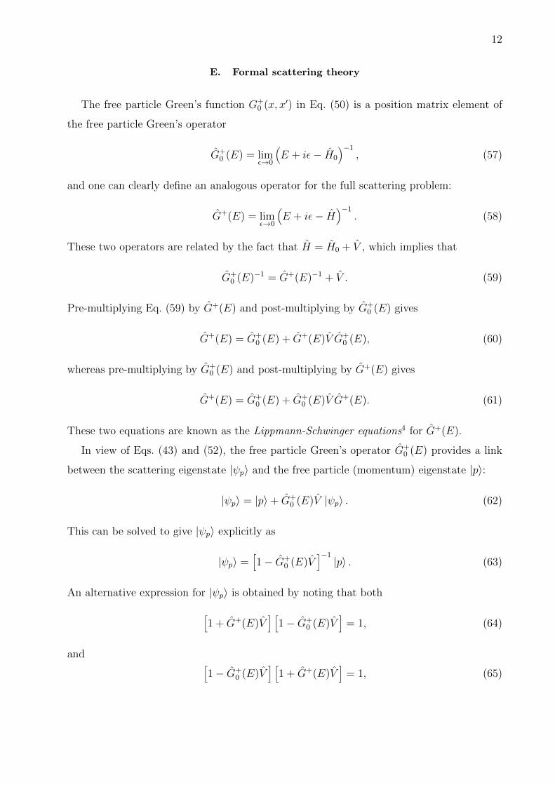
The steps from here to Miller’s trace formula are a series of straightforward manipulations

that begin by replacing |ψp〉 with Ω+ |p〉:

k(T )Qr(T ) =∫ ∞

0dp 〈p| Ω†+e−βH/2F e−βH/2 Ω+ |p〉

=∫ ∞−∞

dp 〈p| Ω†+e−βH/2F e−βH/2 Ω+ |p〉h(p)

=∫ ∞−∞

dp 〈p| Ω†+e−βH/2F e−βH/2 Ω+h(p) |p〉

= tr[Ω†+e

−βH/2F e−βH/2 Ω+h(p)]

= tr[e−βH/2F e−βH/2 Ω+h(p)Ω†+

]. (88)

The physical interpretation of this result is that the rate coefficient can be obtained by

correlating the thermal flux e−βH/2F e−βH/2 through the dividing surface at time t = 0 with

the projection

Ω+h(p)Ω†+ = limt→∞

e−iHt/he+iH0t/hh(p)e−iH0t/he+iHt/h

= limt→∞

e−iHt/hh(p)e+iHt/h (89)

onto states with positive momentum (which are incident on the potential from the reactant

side) in the infinite past.1

C. A simpler projection operator

As it stands, Eq. (88) is already quite appealing. Since the trace can be evaluated in

any convenient basis, we are no longer obliged to solve the Schrodinger equation for the

scattering eigenstates |ψp〉 in order to calculate the reaction rate. And since the equation is

18

guaranteed to give the same result for any choice of dividing surface x = s, we can make this

choice in such a way as to simplify the calculation (as will become apparent when we come on

to consider the classical limit of the equation and its transition state theory approximation

below). However, before we get on to these things, let us spend some time seeing if we can

make Eq. (88) look even prettier than it already is.

The first step in this direction is to note that the projection operator h(p) can be written

equivalently as either2

h(p) = limt→∞

e−iH0t/hh(s− x)e+iH0t/h, (90)

or

h(p) = limt→∞

e+iH0t/hh(x− s)e−iH0t/h, (91)

for any choice of the dividing surface x = s. In other words, positive momentum states

are those that evolve under the influence of the free particle Hamiltonian from the left of

the dividing surface in the infinite past [Eq. (90)] to the right of the dividing surface in the

infinite future [Eq. (91)]. This clearly makes good physical sense, and it can be shown to

be correct by proving that the matrix elements of both sides of Eqs. (90) and (91) are the

same. For example, Eq. (90) can be verified as follows.2

Choosing the position eigenstates as a basis, the matrix elements of h(p) are simply

〈x|h(p) |x′〉 =∫ ∞−∞

dp 〈x|p〉h(p) 〈p|x′〉 =1

2πh

∫ ∞0

dp e+ip(x−x′)/h. (92)

To check that the right-hand side of Eq. (90) has the same matrix elements, we can begin

by writing

〈x| e−iH0t/hh(s− x)e+iH0t/h |x′〉 =∫ ∞−∞

dx′′ 〈x| e−iH0t/h |x′′〉h(s− x′′) 〈x′′| e+iH0t/h |x′〉 . (93)

This contains two free particle propagator matrix elements, which can be shown (see exer-

cise 7 below) to be

〈x| e−iH0t/h |x′′〉 =(

m

2πiht

)1/2

e+im(x−x′′)2/(2ht), (94)

and

〈x′′| e+iH0t/h |x′〉 =(im

2πht

)1/2

e−im(x′′−x′)2/(2ht). (95)

Substituting these results into Eq. (93) and rearranging gives

〈x| e−iH0t/hh(s− x) e+iH0t/h |x′〉 =m

2πht

∫ ∞−∞

dx′′ e+im[(x−x′′)2−(x′′−x′)2]/(2ht)h(s− x′′)

19

=m

2πht

∫ ∞−∞

dx′′ e+im(x+x′−2x′′)(x−x′)/(2ht)h(s− x′′)

=m

2πhte+im(x+x′)(x−x′)/(2ht)

∫ s

−∞dx′′e−imx

′′(x−x′)/(ht), (96)

and changing the integration variable to p = m(s− x′′)/t converts this into

〈x| e−iH0t/hh(s− x)e+iH0t/h |x′〉 = e+im(x+x′−2s)(x−x′)/(2ht) 1

2πh

∫ ∞0

dp e+ip(x−x′)/h

= e+im(x+x′−2s)(x−x′)/(2ht) 〈x|h(p) |x′〉 . (97)

Hence

limt→∞〈x| e−iH0t/hh(s− x)e+iH0t/h |x′〉 = 〈x|h(p) |x′〉 (98)

(for all x, x′ and s), and since the position eigenstate basis is complete this completes the

proof of Eq. (90).

Of Eqs. (90) and (91), Eq. (90) is the more convenient for us, owing to the presence of

the Møller operators Ω+ and Ω†+ in Eq. (89). Indeed combining Eqs. (89) and (90) gives

Ω+h(p)Ω†+ = limt→∞

e−iHt/he+iH0t/he−iH0t/hh(s− x)e+iH0t/he−iH0t/he+iHt/h

= limt→∞

e−iHt/hh(s− x)e+iHt/h, (99)

and inserting this into Eq. (88) gives

k(T )Qr(T ) = limt→∞

[e−βH/2F e−βH/2 e−iHt/hh(s− x)e+iHt/h

]. (100)

This is almost in the neatest possible form, but there is one more useful modification we

can make to it, based on the observation that

h(s− x) = 1− h(x− s). (101)

Since, from Eqs. (39) and (76)

tr[e−βH/2F e−βH/2

]=∑b

〈ψb| e−βH/2F e−βH/2 |ψb〉+∫ ∞−∞

dp 〈ψp| e−βH/2F e−βH/2 |ψp〉

=∑b

e−βEb 〈ψb| F |ψb〉+∫ ∞−∞

dp e−βp2/2m 〈ψp| F |ψp〉 = 0, (102)

the unit operator in Eq. (101) does not contribute to k(T )Qr(T ), and we are left with

k(T )Qr(T ) = − limt→∞

[e−βH/2F e−βH/2 e−iHt/hhe+iHt/h

], (103)

20

.Re p−P

P

Im p

π/4

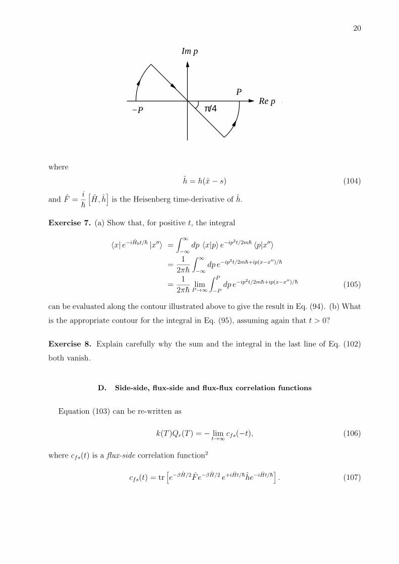
where

h = h(x− s) (104)

and F =i

h

[H, h

]is the Heisenberg time-derivative of h.

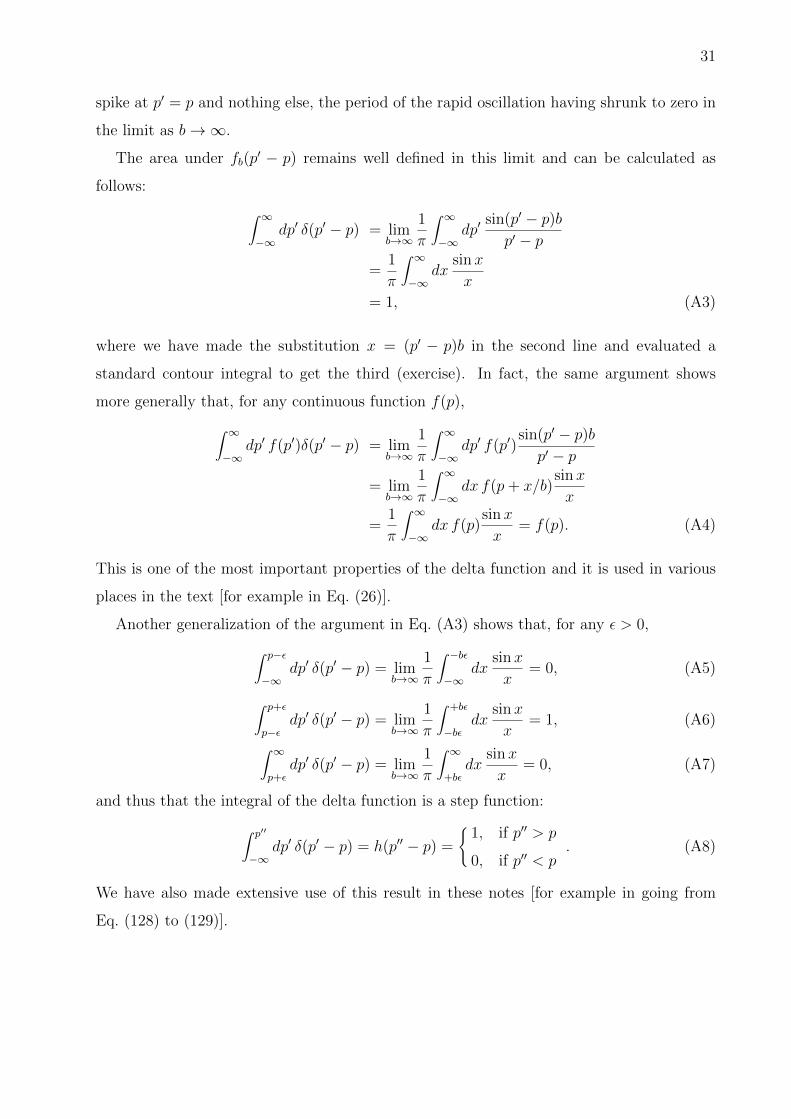
Exercise 7. (a) Show that, for positive t, the integral

〈x| e−iH0t/h |x′′〉 =∫ ∞−∞

dp 〈x|p〉 e−ip2t/2mh 〈p|x′′〉

=1

2πh

∫ ∞−∞

dp e−ip2t/2mh+ip(x−x′′)/h

=1

2πhlimP→∞

∫ P

−Pdp e−ip

2t/2mh+ip(x−x′′)/h (105)

can be evaluated along the contour illustrated above to give the result in Eq. (94). (b) What

is the appropriate contour for the integral in Eq. (95), assuming again that t > 0?

Exercise 8. Explain carefully why the sum and the integral in the last line of Eq. (102)

both vanish.

D. Side-side, flux-side and flux-flux correlation functions

Equation (103) can be re-written as

k(T )Qr(T ) = − limt→∞

cfs(−t), (106)

where cfs(t) is a flux-side correlation function2

cfs(t) = tr[e−βH/2F e−βH/2 e+iHt/hhe−iHt/h

]. (107)

21

Since F =i

h[H, h] is the Heisenberg time derivative of h, one might expect this to be related

to the following side-side

css(t) = tr[e−βH/2he−βH/2 e+iHt/h(1− h)e−iHt/h

](108)

and flux-flux

cff (t) = tr[e−βH/2F e−βH/2 e+iHt/hF e−iHt/h

](109)

correlation functions, and indeed it is. Differentiating Eq. (107) with respect to t immediately

givesd

dtcfs(t) = tr

[e−βH/2F e−βH/2 e+iHt/hF e−iHt/h

]= cff (t), (110)

and differentiating Eq. (108) with respect to t and rearranging gives

d

dtcss(t) = −tr

[e−βH/2he−βH/2 e+iHt/hF e−iHt/h

]= −tr

[e−iHt/hhe+iHt/h e−βH/2F e−βH/2

]= −tr

[e−βH/2F e−βH/2 e−iHt/hhe+iHt/h

]= −cfs(−t), (111)

where we have used the fact that the Boltzmann operator e−βH/2 commutes with the evolu-

tion operators e±iHt/h and that one can cyclically permute the operators within a trace.

These same manipulations reveal that both css(t) and cff (t) are real and even functions

of t. For example,

css(t)∗ = css(−t) = tr

[e−βH/2he−βH/2 e−iHt/h(1− h)e+iHt/h

]= tr

[e−βH h

]− tr

[e−βH/2he−βH/2 e−iHt/hhe+iHt/h

]= tr

[e−βH h

]− tr

[e+iHt/hhe−iHt/h e−βH/2he−βH/2

]= tr

[e−βH h

]− tr

[e−βH/2he−βH/2 e+iHt/hhe−iHt/h

]= tr

[e−βH/2he−βH/2 e+iHt/h(1− h)e−iHt/h

]= css(t), (112)

and similarly for cff (t). In view of Eq. (111), this implies that cfs(t) is a real and odd

function of t, and combining this with Eqs. (106) and (110) gives

k(T )Qr(T ) = limt→∞

d

dtcss(t) = lim

t→∞cfs(t) =

∫ ∞0

dt cff (t). (113)

These final results were originally obtained by Miller et al.2 in 1983. They are entirely rigor-

ous, they apply equally well to more complicated reactions than the simple one-dimensional

22

model problem we have considered here, and they form the basis of all modern approaches

to the calculation of chemical reaction rates.

Exercise 9. (a) Show that css(t) in Eq. (108) can be evaluated as

css(t) =∫ ∞s

dx∫ s

−∞dx′

∣∣∣〈x′| e−iHtc/h |x〉∣∣∣2 , (114)

where tc = t − iβh/2. (b) Now consider the special case where H = H0 and assume that

t > 0 so that 〈x′| e−iH0tc/h |x〉 can be evaluated using Eq. (94). Show that in this case

css(t) =m

2πh|tc|

∫ ∞s

dx∫ s

−∞dx′e−βm(x′−x)2/(2|tc|2). (115)

(c) Prove that, for a > 0, ∫ ∞s

dx∫ s

−∞dx′ e−a(x′−x)2 =

1

2a. (116)

(d) Obtain closed-form expressions for css(t), cfs(t) and cff (t) when H = H0 and sketch

the behaviour of these functions for t between ±3βh. (e) Verify that the rate coefficient

obtained from Eq. (113) agrees with that obtained from Eq. (82) in the special case of free

particle motion.

IV. THE CLASSICAL LIMIT

A. Classical partition functions

There is a straightforward and well-defined procedure for obtaining the classical limit of

a quantum mechanical trace expression such as the definition of cfs(t) in Eq. (107): One

simply replaces the trace with a classical phase space average and all of the operators within

the trace by the corresponding classical functions of positions and momenta.

For example, the classical (high temperature) limit of the partition function for a particle

in a one-dimensional box of length a, which will be familiar from elementary statistical

mechanics courses as

Q(T ) = tr[e−βH

]=∞∑n=1

e−βEn =∞∑n=1

e−βn2π2h2/(2ma2)

∼∫ ∞

0dn e−βn

2π2h2/(2ma2) =1

2

(2πma2

βπ2h2

)1/2

=a

2πh

(2πm

β

)1/2

, (117)

23

can be calculated more directly (without using the quantum mechanical energy levels) as

Q(T ) =1

2πh

∫ ∞−∞

dp∫ ∞−∞

dx e−βH(p,x) (118)

where

H(p, x) =p2

2m+ V (x) (119)

with

V (x) =

0, 0 < x < a,

∞, x < 0, x > a.(120)

Indeed substituting Eqs. (119) and (120) into Eq. (118) immediately gives

Q(T ) =1

2πh

∫ ∞−∞

dp∫ a

0dx e−βp

2/2m =a

2πh

(2πm

β

)1/2

. (121)

B. Classical correlation functions

The classical analogue of the flux operator F in cfs(t) is given by Eq. (36) as

F (p, x) =1

2mδ(x− s)p+ p δ(x− s) =

p

mδ(x− s), (122)

and the classical analogue of the time-evolved side operator

e+iHt/hhe−iHt/h = h[e+iHt/hxe−iHt/h − s

]≡ h[x(t)− s] (123)

is clearly

h(p, x) = h[xt − s], (124)

where xt ≡ xt(p, x) is obtained from p and x by solving the classical equations of motion

pt = −∂H(pt, xt)

∂xt= −dV (xt)

dxt(125)

and

xt = +∂H(pt, xt)

∂pt=ptm

(126)

subject to the initial conditions p0 = p and x0 = x. The classical limit of the rate coefficient

of our model one-dimensional reaction is therefore given by Eq. (113) as

kcl(T )Qr(T ) = limt→∞

cclfs(t), (127)

24

where Qr(T ) = 1/Λ(T ) is the same as in Eq. (83) and

cclfs(t) =

1

2πh

∫ ∞−∞

dp∫ ∞−∞

dx e−βH(p,x) p

mδ(x− s)h(xt − s)

≡ 1

2πh

∫ ∞−∞

dp0

∫ ∞−∞

dx0 e−βH(p0,x0)p0

mδ(x0 − s)h(xt − s). (128)

As in the quantum mechanical case, this classical flux-side correlation function is a real

and odd function of t, and it can be obtained from the time derivative of a classical side-side

correlation function

cclss(t) =

1

2πh

∫ ∞−∞

dp0

∫ ∞−∞

dx0 e−βH(p0,x0)h(x0 − s) [1− h(xt − s)] . (129)

For example, differentiating cclss(t) with respect to t and using Eq. (126) for xt gives

d

dtcclss(t) = − 1

2πh

∫ ∞−∞

dp0

∫ ∞−∞

dx0 e−βH(p0,x0)h(x0 − s)

ptmδ(xt − s), (130)

but in view of Liouville’s theorem (see Appendix C)

dp0 dx0 = dpt dxt, (131)

and the fact that classical dynamics conserves the Boltzmann factor

e−βH(p0,x0) = e−βH(pt,xt), (132)

this can be written equivalently as

d

dtcclss(t) = − 1

2πh

∫ ∞−∞

dpt

∫ ∞−∞

dxt e−βH(pt,xt)h(x0 − s)

ptmδ(xt − s)

≡ − 1

2πh

∫ ∞−∞

dp0

∫ ∞−∞

dx0 e−βH(p0,x0)h(x−t − s)

p0

mδ(x0 − s)

= −cclfs(−t), (133)

which is clearly the classical analogue of Eq. (111).

Exercise 10. Use Eqs. (131) and (132) to prove that cclss(t) is a even function of t. It

follows from this via Eq. (133) that cclfs(t) is an odd function of t, and that the classical rate

coefficient in Eq. (127) can therefore be calculated equivalently as

kcl(T )Qr(T ) = limt→∞

d

dtcclss(t); (135)

again just as in the quantum mechanical case in Eq. (113).

25

C. Classical transition state theory

The classical limit of the flux-side correlation function introduced above is clearly very

similar to its quantum mechanical counterpart. Both are real and odd functions of t and both

are independent of the location of the dividing surface in the limit as t→∞. However, there

is one essential difference between the two that leads to a well-defined classical transition

state theory: cclfs(t) is discontinuous at t = 0 and tends to a non-zero value as t → 0 from

above. In particular, since within the integral in Eq. (128)

limt→0+

δ(x0 − s)h(xt − s) = limt→0+

δ(x0 − s)h(x0 + p0t/m− s)

= limt→0+

δ(x0 − s)h(p0t/m)

= δ(x0 − s)h(p0), (136)

we have

limt→0+

cclfs(t) =

1

2πh

∫ ∞−∞

dp0

∫ ∞−∞

dx0 e−βH(p0,x0)p0

mδ(x0 − s)h(p0)

=1

2πh

∫ ∞0

dp0p0

me−βp

20/2m

∫ ∞−∞

dx0 e−βV (x0)δ(x0 − s)

=1

2πβhe−βV (s), (137)

and inserting this into Eq. (127) in place of limt→∞ cclfs(t) gives the classical transition state

theory result

kTSTcl (T ) =

1

Qr(T )limt→0+

cclfs(t) =

1

2πβhQr(T )e−βV (s) ≡ kBT

h

1

Qr(T )e−βV (s). (138)

Note that:

(a) In undergraduate text books, the transition state theory rate coefficient is usually

written as

kTST(T ) =kBT

h

Q‡(T )

Qr(T )e−∆E‡

0/kBT , (139)

where Qr(T ) is the partition function of the reactants (per unit volume in three di-

mensions or per unit length in one dimension), Q‡(T ) is the partition function of the

transition state excluding the contribution from motion along the reaction coordi-

nate, and ∆E‡0 is the difference in zero point energies between the reactants and the

transition state. For the simple model reaction we are considering here, the reaction

26

coordinate is the only degree of freedom and so Q‡(T ) = 1. And since there is no

zero point energy in any mode orthogonal to the reaction coordinate, ∆E‡0 ≡ V (x‡) is

simply the difference in potential energy between the reactant asymptote and the top

of the reaction barrier at x = x‡ (the “transition state”). So Eq. (138) agrees with

Eq. (139) when we set s = x‡, as it must (because the derivation of Eq. (139) assumes

that the motion along the reaction coordinate is purely classical).

(b) With this choice of dividing surface, the transition state theory approximation in

Eq. (138) will actually give the same result (for our model one-dimensional reaction)

as the full classical rate in Eq. (127). This can be seen by setting s = x‡ in Eq. (128):

cclfs(t) =

1

2πh

∫ ∞−∞

dp0

∫ ∞−∞

dx0 e−βH(p0,x0)p0

mδ(x0 − x‡)h(xt − x‡). (140)

If p0 is positive, a classical trajectory starting at the top of the reaction barrier will

clearly evolve to the right of the barrier as time increases and so make a positive

contribution to the integral in Eq. (140) for t > 0. However, if p0 is negative, the

trajectory will evolve to the left of the barrier and contribute nothing. For any positive

time t, we can therefore replace the step function h(xt − x‡) in the integrand with a

step function in the initial momentum,

δ(x0 − x‡)h(xt − x‡)→ δ(x0 − x‡)h(p0) (t > 0). (141)

Having done this, the same simplifications as in Eq. (137) give

cclfs(t > 0) =

1

2πβhe−βV (x‡) (142)

and therefore

kcl(T ) =1

Qr(T )limt→∞

cclfs(t) =

1

2πβhQr(T )e−βV (x‡) ≡ kBT

h

1

Qr(T )e−βV (x‡). (143)

(c) For any other choice of dividing surface, we will have V (s) ≤ V (x‡), and therefore

e−βV (s) ≥ e−βV (x‡) and [compare Eqs. (138) and (143)]

kTSTcl (T ) ≥ kcl(T ). (144)

This variational aspect of transition state theory carries over to reactions with more

degrees of freedom and enables one to find the optimum dividing surface by minimizing

27

the transition state theory rate (at least in principle; in practice this is quite difficult

to do properly for reactions with more than a handful of degrees of freedom). The

one peculiarity of the one-dimensional case is that the resulting optimized kTSTcl (T ) is

exactly equal to kcl(T ) (as shown above); this is not generally true for reactions with

more degrees of freedom.

Exercise 11. Show by combining Eq. (138) with Eq. (83) that the optimum transition

state theory rate coefficient can be written as

kTSTcl (T ) =

1

2〈|x|〉 e−βV (x‡), (145)

where1

2〈|x|〉 =

∫ ∞0

dpp

me−βp

2/2m/∫ ∞−∞

dp e−βp2/2m (146)

is the thermal expectation value of the classical flux through the dividing surface and the

factor of e−βV (x‡) is the probability that a thermal fluctuation will bring the classical system

to the top of the reaction barrier.

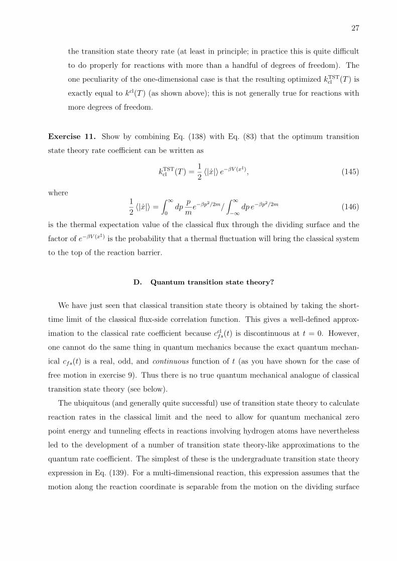
D. Quantum transition state theory?

We have just seen that classical transition state theory is obtained by taking the short-

time limit of the classical flux-side correlation function. This gives a well-defined approx-

imation to the classical rate coefficient because cclfs(t) is discontinuous at t = 0. However,

one cannot do the same thing in quantum mechanics because the exact quantum mechan-

ical cfs(t) is a real, odd, and continuous function of t (as you have shown for the case of

free motion in exercise 9). Thus there is no true quantum mechanical analogue of classical

transition state theory (see below).

The ubiquitous (and generally quite successful) use of transition state theory to calculate

reaction rates in the classical limit and the need to allow for quantum mechanical zero

point energy and tunneling effects in reactions involving hydrogen atoms have nevertheless

led to the development of a number of transition state theory-like approximations to the

quantum rate coefficient. The simplest of these is the undergraduate transition state theory

expression in Eq. (139). For a multi-dimensional reaction, this expression assumes that the

motion along the reaction coordinate is separable from the motion on the dividing surface

28

c (t)/Q (T)fs r

c (t)/Q (T)fs r

classicalrate

exact rate

t t

TST limitNo TST

quantum classical

.

.

.

.

and treats the former classically and the latter quantum mechanically. It therefore includes

zero point energy in the modes orthogonal to the reaction coordinate but it does not allow

for tunneling through the reaction barrier. More sophisticated approximations remove the

separability assumption and include the effect of tunneling, typically in such a way as to

give the exact result for a parabolic barrier. We do not have the time to discuss these

approximations here but some references to them are given in the further reading.1,5,6 The

starting point for the development of new approximations is the exact flux-side correlation

function expression for the quantum rate coefficient in Eq. (113), which underlies most of

the modern research into the theory and calculation of chemical reaction rates.

29

V. FURTHER READING

The material described in these lecture notes is based on two classic papers by Bill Miller,

both of which indicate how the theory can be generalized to treat more complicated reactions

than the simple one-dimensional model problem we have considered here:

1. W. H. Miller, J. Chem. Phys. 61, 1823 (1974).

2. W. H. Miller, S. D. Schwartz and J. W. Tromp, J. Chem. Phys. 79, 4889 (1983).

The two books I found most useful while preparing the lectures were:

3. P. A. M. Dirac, The Principles of Quantum Mechanics, 4th edition (OUP, 1958).

4. J. R. Taylor, Scattering Theory (Dover, 2000).

Three different attempts to construct a quantum mechanical version of transition state

theory are presented in Sec. IV of Ref. 1 and in:

5. G. A. Voth, D. Chandler and W. H. Miller, J. Chem. Phys. 91, 7749 (1989).

6. W. H. Miller, Y. Zhao, M. Ceotto and S. Yang, J. Chem. Phys. 119, 1329 (2003).

And for what it is worth, my own preferred way to calculate chemical reaction rates (includ-

ing quantum mechanical zero point energy and tunneling effects and allowing for recrossing

of the transition state dividing surface) is described in the following two papers, both of

which should be quite accessible to anyone who has understood these lecture notes:

7. I. R. Craig and D. E. Manolopoulos, J. Chem. Phys. 123, 034102 (2005).

8. R. Collepardo-Guevara, I. R. Craig and D. E. Manolopoulos, J. Chem. Phys. 128,

144502 (2008).

30

fb(p’-p)

p’-p

b / π

π / b

VI. APPENDICES

A. The Dirac delta function

The Dirac delta function δ(p′ − p) in Eq. (10) is not a proper mathematical function,3

but it can at least be written as a limit of something that is:

δ(p′ − p) =1

2πh

∫ ∞−∞

dx e−i(p′−p)x/h

= lima→∞

1

2πh

∫ a

−adx e−i(p

′−p)x/h

= lima→∞

1

2πh

[e−i(p

′−p)x/h

−i(p′ − p)/h

]a−a

= lima→∞

1

π

sin(p′ − p)a/h(p′ − p)

= limb→∞

fb(p′ − p), (A1)

where

fb(p′ − p) =

1

π

sin(p′ − p)b(p′ − p)

. (A2)

This function is plotted above. It consists of a sharp peak centred on p′ = p with a height

proportional to b and a width inversely proportional to b, along with a rapid oscillation with

a period of 2π/b that extends to larger values of |p′ − p|. In view of this, the delta function

δ(p′ − p) = limb→∞ fb(p′ − p) can be envisaged as an infinitely high and infinitely narrow

31

spike at p′ = p and nothing else, the period of the rapid oscillation having shrunk to zero in

the limit as b→∞.

The area under fb(p′ − p) remains well defined in this limit and can be calculated as

follows:

∫ ∞−∞

dp′ δ(p′ − p) = limb→∞

1

π

∫ ∞−∞

dp′sin(p′ − p)bp′ − p

=1

π

∫ ∞−∞

dxsinx

x

= 1, (A3)

where we have made the substitution x = (p′ − p)b in the second line and evaluated a

standard contour integral to get the third (exercise). In fact, the same argument shows

more generally that, for any continuous function f(p),

∫ ∞−∞

dp′ f(p′)δ(p′ − p) = limb→∞

1

π

∫ ∞−∞

dp′ f(p′)sin(p′ − p)bp′ − p

= limb→∞

1

π

∫ ∞−∞

dx f(p+ x/b)sinx

x

=1

π

∫ ∞−∞

dx f(p)sinx

x= f(p). (A4)

This is one of the most important properties of the delta function and it is used in various

places in the text [for example in Eq. (26)].

Another generalization of the argument in Eq. (A3) shows that, for any ε > 0,

∫ p−ε

−∞dp′ δ(p′ − p) = lim

b→∞

1

π

∫ −bε−∞

dxsinx

x= 0, (A5)

∫ p+ε

p−εdp′ δ(p′ − p) = lim

b→∞

1

π

∫ +bε

−bεdx

sinx

x= 1, (A6)

∫ ∞p+ε

dp′ δ(p′ − p) = limb→∞

1

π

∫ ∞+bε

dxsinx

x= 0, (A7)

and thus that the integral of the delta function is a step function:

∫ p′′

−∞dp′ δ(p′ − p) = h(p′′ − p) =

1, if p′′ > p

0, if p′′ < p. (A8)

We have also made extensive use of this result in these notes [for example in going from

Eq. (128) to (129)].

32

B. The Heisenberg picture

In the text we have asserted that F = (i/h)[H, h] is the Heisenberg time derivative of h,

and that limt→∞ e−iHt/hh(p)e+iHt/h is the projection onto states with positive momentum

in the infinite past. These assertions are based on the Heisenberg picture of quantum

mechanics, in which state vectors are regarded as time-independent and the time-dependence

is transferred to the operators.

Consider a system with a time-independent Hamiltonian H and a state vector |ψ(t)〉 that

satisfies the time-dependent Schrodinger equation

ihd

dt|ψ(t)〉 = H |ψ(t)〉 . (B1)

Assuming for simplicity that the state |ψ(t)〉 is normalized, the expectation value of an

observable A corresponding to an operator without any explicit time dependence (such as

the projection operator A = h(p)) is given at time t by

A(t) = 〈ψ(t)| A |ψ(t)〉 . (B2)

This is in the Schrodinger picture where the state |ψ(t)〉 evolves in time and the operator A

remains constant.

However, since the Schrodinger equation in Eq. (B1) can be integrated to give

|ψ(t)〉 = e−iHt/h |ψ(0)〉 , (B3)

and therefore

〈ψ(t)| = 〈ψ(0)| e+iHt/h, (B3)

one can equally well write

A(t) = 〈ψ| A(t) |ψ〉 (B4)

where |ψ〉 ≡ |ψ(0)〉 is now constant and

A(t) = e+iHt/hAe−iHt/h (B5)

changes with time. This is the Heisenberg picture, in which A(t) is the Heisenberg-evolved

operator at time t. So for example

limt→∞

e−iHt/hh(p)e+iHt/h = limt→−∞

e+iHt/hh(p)e−iHt/h (B6)

33

can be interpreted as the projection operator onto states with positive momentum (h(p) = 1)

in the infinite past (t→ −∞). And since H commutes with the evolution operators e±iHt/h,

we can differentiate Eq. (B5) with respect to t to obtain

d

dtA(t) =

i

he+iHt/h

[HA− AH

]e−iHt/h

=i

he+iHt/h

[H, A

]e−iHt/h

=i

h

[H, e+iHt/hAe−iHt/h

]=i

h

[H, A(t)

], (B7)

thus confirming that F (t) = (i/h)[H, h(t)] is the Heisenberg time derivative of h(t) (at any

time t including t = 0).

C. Liouville’s theorem

We have made use of Liouville’s theorem in Eq. (131). This theorem states that phase

space volume is conserved in classical mechanics,

dp0 dx0 = dpt dxt, (C1)

or equivalently that the Jacobian of the dynamical transformation from (p0, x0) to (pt, xt)

is unity:

Jt =∂(pt, xt)

∂(p0, x0)=

∣∣∣∣∣ ∂pt/∂p0 ∂xt/∂p0

∂pt/∂x0 ∂xt/∂x0

∣∣∣∣∣ =

(∂pt∂p0

)(∂xt∂x0

)−(∂xt∂p0

)(∂pt∂x0

)= 1. (C2)

Since it is evidently true that J0 = 1, we can prove the theorem by showing that Jt = 0 for

all t, and this follows directly from Hamilton’s equations of motion in Eqs. (125) and (126):

Jt =

(∂pt∂p0

)(∂xt∂x0

)+

(∂pt∂p0

)(∂xt∂x0

)−(∂xt∂p0

)(∂pt∂x0

)−(∂xt∂p0

)(∂pt∂x0

)

=

(∂pt∂p0

)(∂xt∂x0

)−(∂pt∂x0

)(∂xt∂p0

)−(∂xt∂p0

)(∂pt∂x0

)+

(∂xt∂x0

)(∂pt∂p0

)

= −(∂H

∂xt

)[(∂xt∂p0

)(∂xt∂x0

)−(∂xt∂x0

)(∂xt∂p0

)]

−(∂H

∂pt

)[(∂pt∂p0

)(∂pt∂x0

)−(∂pt∂x0

)(∂pt∂p0

)]= 0. (C3)