Chemical Methods for Ugnu Viscous Oils - National … library/research/oil-gas...1 Chemical Methods...

1

Chemical Methods for Ugnu Viscous Oils

Project Number: DE-NT0006556

Final Report

Period Covered: October, 2008-March, 2012

for U. S. Department of Energy

National Energy Technology Laboratory

Principal Investigator: Kishore K. Mohanty Department of Petroleum & Geosystems Engineering

University of Texas at Austin CPE-3.168, 1 University Station, Mail Code C0300

Austin, Texas 78712 512-471-3077 (phone), 512-471-9605 (fax)

[email protected]

June 5, 2012

mailto:[email protected]�

2

Disclaimer

This report was prepared as an account of work sponsored by an agency of the United States

Government. Neither the United States Government nor any agency thereof, nor any of their

employees, makes any warranty, express or implied, or assumes any legal liability or

responsibility for the accuracy, completeness, or usefulness of any information, apparatus,

product, or process disclosed, or represents that its use would not infringe privately owned rights.

Reference herein to any specific commercial product, process, or service by trade name,

trademark, manufacturer, or otherwise does not necessarily constitute or imply its endorsement,

recommendation, or favoring by the United States Government or any agency thereof. The

views and opinions of authors expressed herein do not necessarily state or reflect those of the

United States Government or any agency thereof.

3

TABLE OF CONTENTS

Page

Cover Page 1

Disclaimer 2

Table of Contents 3

Executive Summary 4

Introduction 6

Methodology 9

Results and Discussion 19

Surfactant Screening for the Viscous Oil 19

Surfactant Screening for the Heavy Oil 25

1D Sand Pack Floods of the Viscous Oil 32

1D Sand Pack Floods of the Heavy Oil 38

2D Floods of the Viscous Oil 44

2D Floods of the Heavy Oil 45

Micromodel Studies 55

Modeling of Oil Displacement 65

Technology Transfer 76

Future Directions 77

Conclusions 78

Acknowledgement 81

References 82

4

Executive Summary

The North Slope of Alaska has large (about 20 billion barrels) deposits of viscous oil in

Ugnu, West Sak and Shraeder Bluff reservoirs. These shallow reservoirs overlie existing

productive reservoirs such as Kuparuk and Milne Point. The viscosity of the Ugnu reservoir on

top of Milne Point varies from 200 cp to 10,000 cp and the depth is about 3300 ft. The same

reservoir extends to the west on the top of the Kuparuk River Unit and onto the Beaufort Sea.

The depth of the reservoir decreases and the viscosity increases towards the west. Currently, the

operators are testing cold heavy oil production with sand (CHOPS) in Ugnu, but oil recovery is

expected to be low (< 10%). Improved oil recovery techniques must be developed for these

reservoirs. The proximity to the permafrost is an issue for thermal methods; thus nonthermal

methods must be considered.

The objective of this project is to develop chemical methods for the Ugnu reservoir on

the top of Milne Point. An alkaline-surfactant-polymer (ASP) formulation was developed for a

viscous oil (330 cp) where as an alkaline-surfactant formulation was developed for a heavy oil

(10,000 cp). These formulations were tested in one-dimensional and quarter five-spot Ugnu sand

packs. Micromodel studies were conducted to determine the mechanisms of high viscosity ratio

displacements. Laboratory displacements were modeled and transport parameters (such as

relative permeability) were determined that can be used in reservoir simulations.

Ugnu oil is suitable for chemical flooding because it is biodegraded and contains some

organic acids. The acids react with injected alkali to produce soap. This soap helps in lowering

interfacial tension between water and oil which in turn helps in the formation of macro and micro

emulsions. A lower amount of synthetic surfactant is needed because of the presence of organic

acids in the oil.

Tertiary ASP flooding is very effective for the 330 cp viscous oil in 1D sand pack. This

chemical formulation includes 1.5% of an alkali, 0.4% of a nonionic surfactant, and 0.48% of a

polymer. The secondary waterflood in a 1D sand pack had a cumulative recovery of 0.61 PV in

about 3 PV injection. The residual oil saturation to waterflood was 0.26. Injection of tertiary

alkaline-surfactant-polymer slug followed by tapered polymer slugs could recover almost 100%

of the remaining oil. The tertiary alkali-surfactant-polymer flood of the 330 cp oil is stable in

three-dimensions; it was verified by a flood in a transparent 5-spot model. A secondary polymer

flood is also effective for the 330 cp viscous oil in 1D sand pack. The secondary polymer flood

5

recovered about 0.78 PV of oil in about 1 PV injection. The remaining oil saturation was 0.09.

The pressure drops were reasonable (<2 psi/ft) and depended mainly on the viscosity of the

polymer slug injected.

For the heavy crude oil (of viscosity 10,000 cp), low viscosity (10-100 cp) oil-in-water

emulsions can be obtained at salinity up to 20,000 ppm by using a hydrophilic surfactant along

with an alkali at a high water-to-oil ratio of 9:1. Very dilute surfactant concentrations (~0.1 wt%)

of the synthetic surfactant are required to generate the emulsions. It is much easier to flow the

low viscosity emulsion than the original oil of viscosity 10,000 cp. Decreasing the WOR reverses

the type of emulsion to water-in-oil type. For a low salinity of 0 ppm NaCl, the emulsion

remained O/W even when the WOR was decreased. Hence a low salinity injection water is

preferred if an oil-in-water emulsion is to be formed.

Secondary waterflood of the 10,000 cp heavy oil followed by tertiary injection of

alkaline-surfactants is very effective. Waterflood has early water breakthrough, but recovers a

substantial amount of oil beyond breakthrough. Waterflood recovers 20-37% PV of the oil in 1D

sand pack in about 3 PV injection. Tertiary alkali-surfactant injection increases the heavy oil

recovery to 50-70% PV in 1D sand packs. As the salinity increased, the oil recovery due to

alkaline surfactant flood increased, but water-in-oil emulsion was produced and pressure drop

increased. With low salinity (deionized) water, the oil recovery was lower, but so was the

pressure drop because only oil-in-water emulsion was produced. Secondary waterflood of the

10,000 cp heavy oil in 5-spot sand packs recovers 30-35% OOIP of the oil in about 2.5 PV

injection. Tertiary injection of the alkaline-surfactant solution increases the cumulative oil

recovery from 51 to 57% OOIP in 5-spot sand packs. As water displaces the heavy oil, it fingers

through the oil with a fractal structure (fractal dimension = 1.6), as seen in the micromodel

experiments. Alkaline-surfactant solution emulsifies the oil around the brine fingers and flows

them to the production well. A fractional flow model incorporating the effect of viscous

fingering was able to match the laboaratory experiments and can be used in reservoir simulators.

The chemical techniques look promising in the laboratory and should be tested in the fields.

6

Introduction

The North Slope of Alaska has large (about 20 billion barrels) deposits of viscous oil in

Ugnu, West Sak and Shraeder Bluff reservoirs. These shallow reservoirs overlie existing

productive reservoirs such as Kuparuk and Milne Point. The viscosity of the Ugnu reservoir on

top of Milne Point varies from 200 cp to 10,000 cp (Seccombe et al., 2005). The average depth is

about 3300 ft, pressure about 1600 psi, and temperature about 75 °F. The same reservoir extends

to the west on the top of the Kuparuk River Unit and onto the Beaufort Sea. The depth of the

reservoir decreases and the viscosity increases towards the west.

The Ugnu reservoir has two major sand intervals: M- and L- sands. They were formed in

late Cretaceous through lower Tertiary and are stacked fluvial to deltaic. The sands are

unconsolidated and permeabilities range from hundreds of millidarcy to several darcy. The upper

sand is about 300 ft thick and consists of several thick sand bodies. The lower sand is about 200

ft thick and contains several thinner sand bodies. There are many faults which divide the

reservoir into many blocks with differing oil type and viscosity. Oil viscosity varies from several

hundreds to millions of cp.

Many thermal methods have been considered for oil recovery from Ugnu, e.g., steam

flooding, SAGD, in situ combustion, electrical heating, and electromagnetic heating. The key

problem in implementing thermal recovery in Ugnu is the proximity of the reservoir to

permafrost. Heat from the reservoir could be conducted to the permafrost and start melting it

leading to geomechanical and environmental problems. Heat in the wellbore can also cause

similar problems if steam is injected from the surface and wellbores are not insulated. Thus non-

thermal methods must be considered along with thermal methods.

Waterflooding is a common and inexpensive secondary oil recovery technique for light

oils. For viscous oils, the adverse mobility ratio between the water (~1 cp) and the oil (~10,000

cp) phase severely hampers the performance of the waterflood. Water fingers through the oil

phase and leaves most of the oil behind leading to poor recoveries (Bryan, 2008; Jennings, 1966;

Kumar, 2005; Miller, 2006). Previous research (Bryan, 2008) has shown that the oil recovery can

be improved by the application of alkali surfactant (AS) flooding. This work focuses on the

application of this technique for heavy Alaskan oil.

If the oil viscosity is a few hundred cp, then it may be possible to displace the oil by a

chemical bank in a stable manner at a fast enough rate. If the oil viscosity is 10,000 cp or higher,

7

a stable displacement velocity would be very low to be economic. In such cases, we propose an

unstable waterflood followed by a chemical flood. The unstable waterflood would create fingers

and pressure drop would be small after breakthrough. If the oil can be produced through these

fingers, then the pressure drop would stay low.

Surfactants are organic molecules having a hydrophilic head and a hydrophobic tail. They

are called amphiphilic and the balance of hydrophilic and the hydrophobic character (HLB)

depends on the molecular structure of surfactants (Rekvig, 2003). Alkalis can react with the acids

present in the crude oil to form in-situ soaps. The soap molecules also act as surface active

agents and hence can reduce the requirement of synthetic surfactants (Martin, 1985; Thomas,

2001; Hirasaki, 2008). Surfactants, whether synthetic or soap molecules made by alkali, reduce

interfacial tension between water and oil. Reduction in interfacial tension can lead to an increase

in capillary number which can reduce residual oil saturation to a sufficiently low value.

Traditional tertiary chemical flooding of light oil reservoirs use this mechanism (Healy & Reed,

1977; Nelson & Pope, 1978; Pope et al., 1979; Flaaten et al., 2008).

Pioneering work on surfactant-polymer flooding was performed in 1970s when the key

factors influencing the process were identified (Healy and Reed, 1977; Salager et al., 1979;

Bennett et al., 1981). The oil/brine/surfactant phase behavior was identified as type I (oil in water

microemulsion), type II (water in oil microemulsion) or type III (middle phase microemulsion)

which exhibits the lowest IFT (Winsor, 1954). Cosurfactant enhanced alkali flooding (Nelson

1978) was introduced which allowed increasing the optimal salinity of the alkali slug high

enough for its satisfactory propagation. The phase behavior of oil-brine-surfactant systems would

often be accompanied by viscous emulsions, gels or liquid crystals (Hackett and Miller,1988;

Levitt et al., 2009). Cosolvents are often added for avoiding the formation of these structured

phases. Most of the surfactant flooding research in 1970s and 1980s were limited to sandstones

with low salinity. Recent research has led to the development of surfactant systems suitable for

high salinity and carbonate environments (Levitt et al., 2009; Barnes et. al., 2008; Hirasaki et al.,

2008; Adibhatla & Mohanty, 2008). Several ASP field tests have also confirmed that the residual

oil can be displaced by the use of alkaline-surfactant-polymer system (Falls et al., 1992; Reppert

et al., 1990). In particular, the ASP field test in the Daqing field recovered about 20% additional

OOIP after waterflooding (Shutang et al., 2010).

8

Alkaline-surfactant-polymer techniques have been studied for mostly light oils in the past

(Nelson & Pope 1978; Flatten et al. 2008). Here we extend its application to the viscous oil

reservoirs. Polymer floods have been considered for viscous oil reservoirs for a long time

(Seright 2010, Wassmuth et. al. 2007), but they do leave behind a residual oil saturation. Alkali

surfactant formulations have been recently developed for a few viscous oils (Yang et. al. 2010),

where the remaining oil saturations have been reduced to very little. In this study, we develop an

alkaline-surfactant-polymer formulation for a viscous oil of 330 cp at 25°C.

The key problem in heavy oil (~10,000 cp) reservoir is inefficient sweep due to low

mobility of the oil. If the injected alkali-surfactant solutions can form oil-in-water (O/W)

emulsions, the viscosity of these emulsions would be much lower than that of the original oil.

Thus the bypassed oil can be emulsified at the surface of the water fingers, mobilized and

produced at relatively low pressure gradients (Liu, 2006). Generally speaking, addition of highly

hydrophilic surfactants (high HLB), low salinity, and high WOR lead to O/W emulsions (Bryan,

2007). The goal of this work is to identify chemicals for forming oil-in-water emulsions with a

heavy Alaskan oil and conduct displacement studies to understand the recovery of heavy oils.

This work deals with two oils: a 330 cp oil (referred to as a viscous oil) and a 10,000 cp oil

(referred to as a heavy oil).

9

Methodology

Surfactant Screening

Surfactant screening experiments were performed to identify the surfactant-alkali

combinations which could generate large oil and water solubilizations and thus ultra low

interfacial tensions (IFT) with a viscous oil (330 cp). The reservoir temperature ranges from 15

to 30oC and thus the experiments were performed at the room temperature (25oC). Due to the

high organic acid content of the crude oil, an alkali was used to generate in situ soaps. Formation

brine has low salinity (20,000 ppm NaCl) and negligible divalent ions such as calcium and

magnesium; thus sodium carbonate is used as the alkali. In addition to the alkali, a synthetic non-

ionic surfactant was added to bring the optimum salinity to the desired level. The in situ

generated soap lowers the requirement of the externally added surfactant. The amount of in situ

generated soaps is in turn dependent on the volume ratio of water and oil (WOR) in the system

(Nelson 1978). Prescribed amounts of water, oil, alkali, and surfactant were mixed at different

water-to-oil ratio (WOR) and the volumes of equilibrium phases were observed. The activity

diagram is then constructed showing the Type I, II or III regions at different WOR. Samples

were equilibrated in test tubes (not pipettes) because the viscosity of the oil is quite high.

Several surfactants were tested in our lab to identify those which can form low viscosity

oil-in-water (O/W) emulsions with the heavy reservoir oil. The heavy reservoir oil has a

viscosity of 10,000 cp and an acid number of 3.54 mg KOH/100 gm of oil. Because the oil has a

high acid number, an alkali was chosen to produce in situ soaps. Soaps act as in situ surfactants

and minimize the requirement for expensive synthetic surfactants. Three relatively hydrophilic

surfactants: Bioterge, Tergitol 15-S-20, and TDA-30EO were used. Bioterge is sodium C14-16

olefin sulfonate. Tergitol 15-S-20 is a secondary alcohol ethoxylate. TDA-30EO is a Tridecyl

alcohol with 30 ethoxy groups. The first surfactant is anionic, but the other two are nonionic.

Surfactant concentration was kept low at 0.1% by active weight. Reservoir salinity varies from

8900 to 20,000 ppm and consists of mostly NaCl. Initial screening tests were carried out at a

constant WOR (water-to-oil ratio) of 9:1. Because of the absence of divalent ions, sodium

carbonate (Na2CO3) was chosen as the alkali. Surfactant and alkali were added to the NaCl brine

and then mixed with reservoir oil in glass vials. The samples were mixed thoroughly and allowed

to stand for 1 week or more to allow the phases to separate at the room temperature, ~25oC. The

10

amount of the emulsion phase was observed and in some cases, the viscosity of the emulsion

phase was measured by a Brookfield DVII+ viscometer.

Sand Pack Floods

Sand pack floods were conducted in order to assess the surfactant system and identify the

parameters governing the oil recovery for both the viscous and the heavy oils. In order to prepare

the sand pack, the reservoir sand was washed and packed in a thin 3 feet long steel tube having

an inside diameter of 2/3 inches. Porosity was about 30-35 %. Permeability of the pack (20-25

D) was determined by flowing brine through it and measuring the pressure drop across the pack

using a Honeywell pressure transducer. Oil was injected inside the sand pack at high pressure

(~300 psi) until no more water was seen at the outlet. The irreducible water saturation was

measured to be ~10% of the total pore volume. The sand pack saturated with oil was kept at a

high temperature (~80oC) for ~10 days to let the oil adsorb on the sand surface. After this period,

it was kept at the room temperature for 2-3 days to cool down.

Figure 1: Sand pack flood set-up

∆P

2/3 inch

Sample Collectorr

11

The set up for the sand pack flood is shown in Figure 1. The displacing fluid is pumped

at a constant flow rate through an ISCO pump. The pressure drop across the tube is measured

and the samples are collected in a tube sampler in order to measure oil recovery as a function of

time. The flow rates were kept low in order to mimic the field rates. Water was injected for about

3-4 PV followed by the injection of an alkali-surfactant solution at the same flow rate for another

2-3 PV. The salinity of these floods was varied from 0 to 20,000 ppm NaCl. These floods were

conducted at the room temperature. An alkali surfactant formulation of 0.1% TDA 30EO, 0.5%

Na2CO3 alkali was tested in 1D sand pack floods of the heavy oil. All the floods were performed

in the tertiary mode where the AS solution was injected after the brine injection. Table 1

provides the properties of the sand pack.

Table 1: Properties of the sand pack

Porosity (Ф) 42.3%

Permeability (k) 22.6 Darcy

Connate Water Saturation

(Swc)

8.6%

2D Sand Pack Floods

Two kinds of 2D cells were used in our experiments. The first kind was a transparent

(plastic) cell that allowed visual observation of the flow paths at the top of the cell. This cell was

square shape with sides measuring 10 inches and the thickness of 0.8 inches. The fluids were

injected at one corner and collected from the diagonally opposite corner. Once we were

convinced that viscous fingers are forming in the porous medium, we switched to an opaque

(steel) 2D cell which had a higher pressure rating than the transparent model. The thickness of

this cell was 1 inch. All the other dimensions were same as the first cell. The second cell had the

provision to apply an overburden pressure on the sandpack.

Different sand pack preparation methods were followed for the two cells. In the

transparent model sand was packed in the dry state and in the opaque model in the wet state. Dry

12

packing of sand enabled us to determine the pore volume by vacuuming followed by water

saturation. However, it was difficult to achieve a low porosity pack and on pressurizing the pack

to 30-40 psi, we could observe some gaps in the pack. These gaps were refilled until no more

gaps were seen even after pressurizing the pack. The opaque cell was packed wet with the sand.

Wet packing gave a tighter pack and the overburden pressure applied to the cell kept the sand

from moving inside.

Table 2. Properties of quarter 5-spot sand packs

Nitrogen and brine porosity were measured for the dry pack. However for the wet pack

the brine pore volume was measured by measuring the amount of brine eliminated by the pack

once the overburden pressure is applied and subtracting it from the measure of the amount of

brine initially used to wet the sand to be packed inside. Another check of pore volume was

performed by conducting a brine tracer test on this pack. The properties of the sand packs are

given in Table 2. Permeability was measured by injecting brine at a particular flow rate and

measuring the pressure drop across the pack. Air permeability and brine permeability were

measured for the transparent pack and only brine permeability was measured for the wet pack.

Sand pack

Type

Bulk Volume

Porosity

Permeability

(ml) (%) (Darcy)

1 Transparent 1310.97 53.17 18.8

2 Opaque 1638.71 24.40 11.1

Fraction collector

10 inches

∆P

Brine/ AS solution

Quarter 5 spot cell

13

Figure 2. Setup of the 2D sand pack

Oil was injected into the water saturated packs until the water saturation was reduced to

about 10-14%. Oil was heated to 60 ºC to reduce its viscosity during the oil saturation in order to

speed up the process. The sand pack flood setup is shown in Figure 2. The injection fluid is

pumped at a constant flow rate through an ISCO pump. The pressure drop across the pack is

measured and the samples are collected in a tube sampler in order to measure oil recovery as a

function of time. A flow rate of 0.1 ml/min was selected for all the floods. Water was injected for

about 2.5 PV followed by the injection of an alkali-surfactant solution at the same flow rate for

another 2.4 PV. The salinity of these floods was varied from 2000 to 20,000 ppm NaCl. These

floods were conducted at the temperature of 25 ºC. A polymer flood was conducted in a steel 2D

cell model and the results are compared with the brine flood conducted in the same pack.

Micromodel

The experiments were conducted in a two-dimensional porous medium (micro-model)

etched on a silicon plate. Such micromodels have been extensively used in pore-scale petroleum

engineering research as a surrogate porous medium (Sun et al., 2004; Alshehri et al., 2009). A

pore pattern was etched on a 5cm X 5 cm silicon wafer. Average etching depth was about 25 µm

and average pore throat size was approximately 50 µm. A transparent glass plate covering the

etched surface enables the visualization of oil and water movements using a reflection

microscope. Figure 3(a) below shows a picture of the pores of the micromodel. To prepare the

micromodel for the water flooding experiment, we followed the procedure conventionally used

for core flooding experiments as closely as possible, keeping in mind the pressure and force

limits of our system. The micromodel was first vacuumed by pumping the air out with a syringe.

Once the piston of the syringe can no longer be drawn further, the valve on the other end of the

flow cell was opened. The synthetic reservoir brine rushed in and saturated the system. Oil was

then injected to displace the brine. This oil saturated system (with some connate water) was used

for water flooding experiments. Figure 3(b) shows the micromodel and the flow scheme used

during the experiments. The fluids were injected at the top left corner and produced from the

bottom right corner. There was a wide flow channel on the top to distribute the fluids across the

14

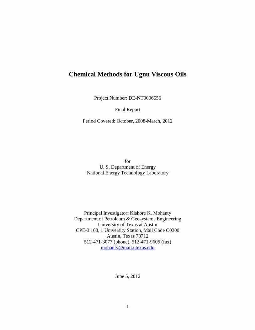
width (and a similar channel at the bottom). The experimental setup is shown in the Figure 4. A

microinjection pump was used to pump the liquid in the model at a constant rate of 5µl/min. This

rate corresponds to a velocity of approximately 2.5 ft/d for our micromodel.

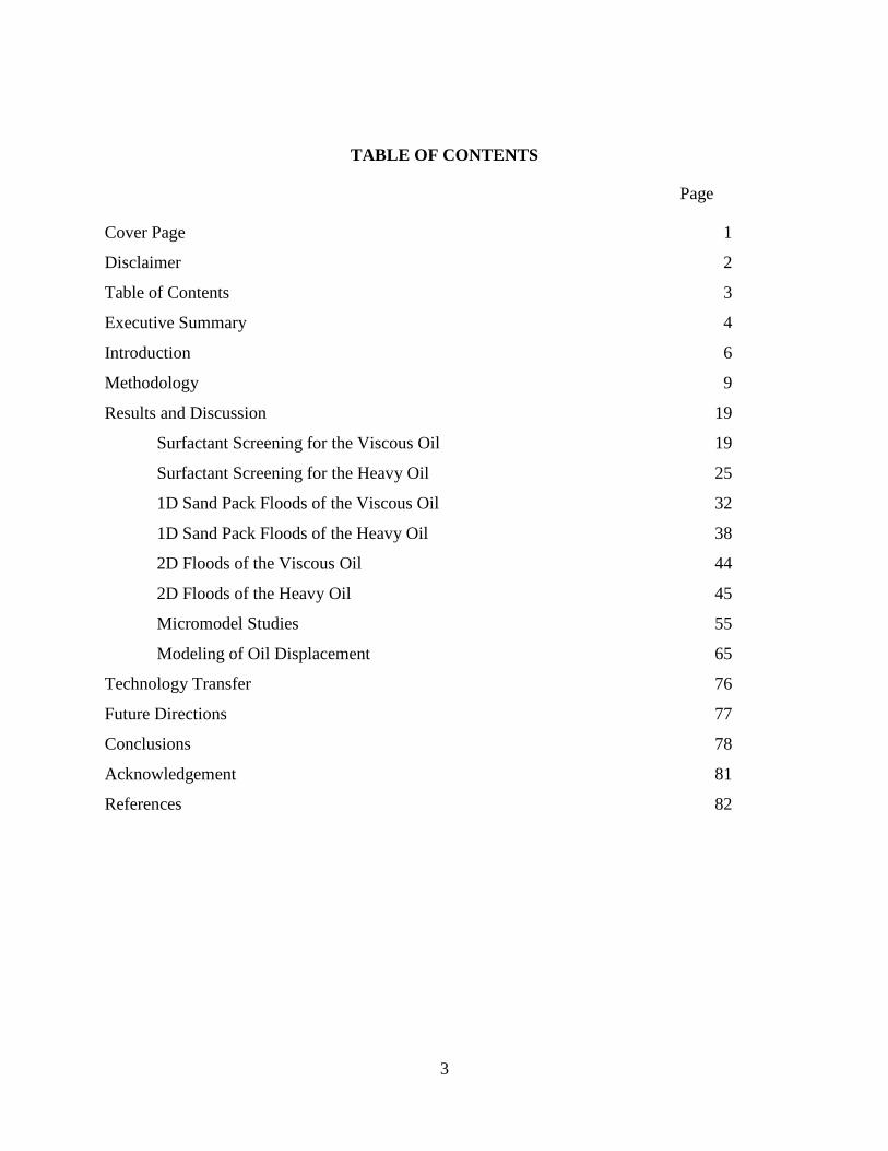
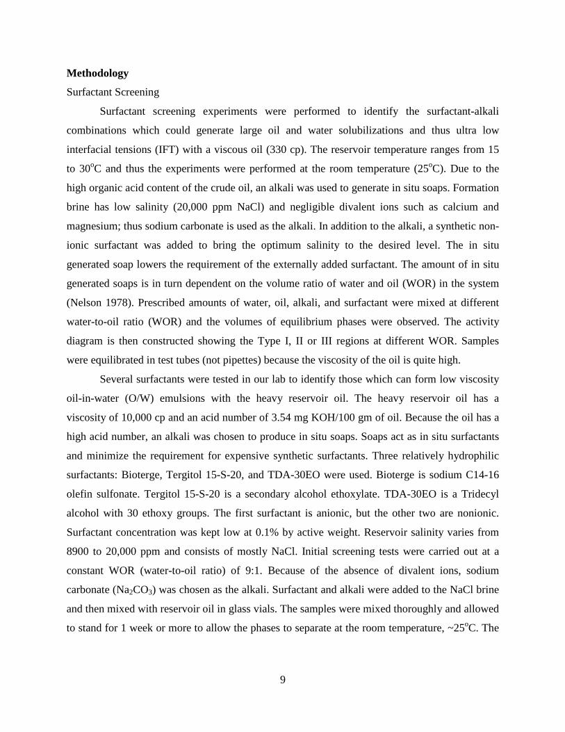
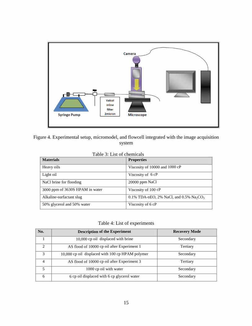
Table 3 presents the list of materials used in our experiments. Six experiments were

conducted and they are listed in Table 4. The experiments were recorded using a video camera.

However, when higher resolution and pore level details were required, the setup was moved to

the stage of a microscope. The microscope had the capability to capture still images at a high

resolution.

DLA simulations were conducted to study the similarity of the fingers formed in our

micromodels with those generated by the DLA method. The code for the simulation was written

in MATLAB. The algorithm of DLA is as follows: we start with an occupied site (or seed) of a

lattice located at the injection point. Random walkers are released, one at a time far from the

seed site and are allowed to move randomly in the lattice. If a walker comes to an empty site

adjacent to an occupied site, then the empty site is occupied and the aggregate of the occupied

sites advances by one site. This walker is then removed and a new walker is released. For our

study, we simulated the DLA structures for a line seed and a point seed.

Figure 3(a). Microscopic view of a 1.8 mm X 1.3 mm section of the micromodel showing the etched

pore pattern

Figure 3(b). Micromodel and flow scheme: injection is from top left corner and production is from bottom right, flow channel distributes the liquid uniformly at the inlet

600 μm

15

Figure 4. Experimental setup, micromodel, and flowcell integrated with the image acquisition system

Table 3: List of chemicalsaterials

Materials Properties

Heavy oils Viscosity of 10000 and 1000 cP

Light oil Viscosity of 6 cP

NaCl brine for flooding 20000 ppm NaCl

3000 ppm of 3630S HPAM in water Viscosity of 100 cP

Alkaline-surfactant slug 0.1% TDA-nEO, 2% NaCl, and 0.5% Na2CO3

50% glycerol and 50% water Viscosity of 6 cP

Table 4: List of experiments No. Description of the Experiment Recovery Mode

1 10,000 cp oil displaced with brine Secondary

2 AS flood of 10000 cp oil after Experiment 1 Tertiary

3 10,000 cp oil displaced with 100 cp HPAM polymer Secondary

4 AS flood of 10000 cp oil after Experiment 3 Tertiary

5 1000 cp oil with water Secondary

6 6 cp oil displaced with 6 cp glycerol water Secondary

16

The images and videos captured were later analyzed to calculate the fractal dimensions of

the fingers. The fractal nature of the fingers gives us a basis to compare different patterns formed

at different viscosity ratios and capillary numbers. The classic signature of a fractal is a non-

Euclidean relationship between mass and size. For an ordinary circular or rectangular two

dimensional object, mass is proportional to R2. Similarly, for a cube or a sphere, mass is

proportional to R3, but for a two- or three-dimensional fractal object the mass is proportional to

RDf, where Df is a non-integer number, less than the Euclidean dimension of the object.

Calculating the fractal dimension of the viscous fingers helps in understanding the impact of

viscosity ratio on the finger shapes and its similarity to the DLA model. Fractal dimension can be

calculated by the “box counting” method. Box counting utilizes the fact that fractals display self-

similarity and can be split into parts, each of which is (at least approximately) a reduced-size

copy of the whole. According to this method, the number of boxes of size R needed to cover

a fractal set follows a power-law,

…………(1)

where ≤ D (D is the Euclidean dimension of the space, usually D = 1, 2, 3). Thus,

…………(2)

More accurately,

…………(3)

is also known as the Minkowski-Bouligand dimension, or Kolmogorov capacity, or

Kolmogorov dimension, or simply box-counting dimension.

Modeling of Unstable Flow

Assumptions of the model

1) The displacement process is 1D in character.

2) Flow characteristics in different viscous fingers can be represented by one viscous finger.

3) The representative viscous finger has a cross sectional area which remains constant with

time, position and saturations.

17

4) The representative viscous finger does not exchange fluids (oil or water) with the

unfingered zone.

5) Single phase oil flow is allowed to occur in the unfingered zone. Two phase flow occurs

in the viscous finger.

Figure 5. Sketch of immiscible viscous fingers

The green region represents the oil and the blue region represents the water in Figure 5. The

fractional cross sectional area of the finger is represented by ‘f’. Thus the fingered cross sectional

area is equal to ‘Af’.

Calculation of the Oil Production Performance

As the two phase flow is allowed to occur in the finger, we can write the following

expressions for the oil and the water flow rates by using the Darcy law.

rww

w

kk Af Pqxµ

∂ = − ∂ ----------------------------------------------------------------- (4)

(1 )oro ro

oo o

kk Af kk A fP Pqx xµ µ

−∂ ∂ = − + − ∂ ∂ -------------------------------------------(5)

where 1

Ewfo

rw rw

Sw Swik k

Swi Sorw−

= − − -------------------------------------------------- (6)

& 11

Eofo

ro ro

Sw Sorwk k

Swi Sorw− −

= − − ------------------------------------------------- (7)

Water

2 phase flow in the finger

Single phase oil flow in the unfingered zone

Swf: Water saturation inside the finger Swi: Initial water saturation in the finger Sorw: Residual oil saturation in the finger

18

The model uses Correy correlations to describe the relative permeabilities of oil and

water in the finger. The saturation values used in the expressions are also the ones prevailing in

the finger. The total amount of fluid passing the cross section is

w oq q q= + ------------------------------------------------------------------------------- (8)

The fractional flow of water through the cross section can be written as:

ww

w o

qfq q

=+

------------------------------------------------------------------------------ (9)

Buckley Leverett 1D model is used to determine the cumulative oil recovery with time.

Before breakthrough, d dNp t= -------------------------------------------------------- (10)

After breakthrough, (1 )wd w wi

w

w

fNp S SdfdS

−= − +

, 1d

w

w

tdfdS

=

------------------- (11)

Npd: Cumulative Pore Volumes of oil produced

td: Cumulative Pore Volumes of water injected

Sw: Water saturation averaged over the cross section of the sandpack.

(1 )(1 )w wf wiS S f S f= + − − ------------------------------------------------------------ (12)

Calculation of the pressure drop across the formation

The pressure drop across the formation can be calculated from the Darcy law.

1

0 (1 )

Do

rw ro ro

w o o

dxqLPkA k k kf f

µ µ µ

∆ =

+ + −

∫ , xD = dimensionless distance = x/L ------------ (13)

Reservoir simulator, CMG was also used to numerically model the laboratory experiments and

field-scale flow.

19

Results and Discussion

Surfactant Screening for the Viscous Oil

Phase behavior of surfactant-alkali-oil-brine mixtures was first studied as a function of

the surfactant concentration at a fixed alkali (0.5 wt%) and salt (20,000 ppm NaCl)

concentration. Figure 6 shows the phase behavior when the surfactant concentration increases

from 0 to 0.9 wt% in the increments of 0.1 wt% at 25 °C. No polymer was present in these phase

behavior test tubes; water oil ratio (WOR) was fixed at 1. The samples with 0 and 0.1 wt%

surfactant showed viscous emulsions at the bottom of the oil phase. This was confirmed because

the lower phase did not move when the tubes were tilted. On the other hand, the samples with

higher amounts of the surfactant did not show the presence of any viscous emulsion. Samples

with 0.3% and 0.4% surfactant started to show a thin layer of the third phase. On tilting the

tubes, all the phases showed good fluidity. Samples with higher surfactant concentration showed

higher volumes of the 3rd phase. This surfactant also acts as a cosolvent and gives fluidity to the

middle phase. Phase behavior was then studied as a function of the alkali concentration at fixed

surfactant concentrations.

Figure 6: Phase behavior with 0.5 wt% alkali and 20,000 ppm brine with varying surfactant

concentration from 0 wt % on the left to 0.9 wt% on the right

20

Figure 7 shows the phase behavior of samples with a (low) 0.1wt% surfactant

concentration in 20,000 ppm NaCl brine and varying alkali concentrations at 25 °C. Three phases

develop, but all the samples show the presence of viscous emulsions at the bottom of the oil

phase. These observations are consistent with those of Figure 2 where these viscous emulsions

were observed for low surfactant concentrations.

Figure 7: Phase behavior of samples with 0.1 wt% surfactant and 20,000 ppm NaCl with varying

alkali concentration (alkali concentration varies from 0 wt% on the left to 0.8 wt% on the right)

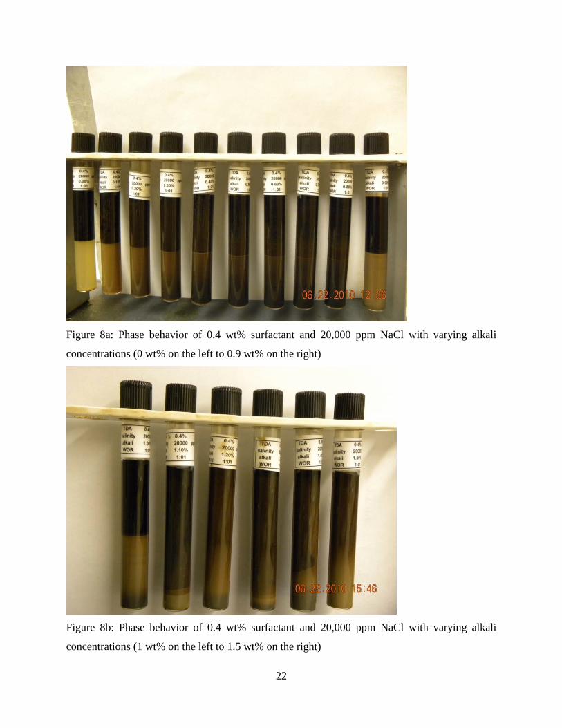
Figure 8 shows the phase behavior of samples with 0.4 wt% (high) surfactant and

20,000ppm NaCl brine at a WOR of 1:1 and 25 °C. The alkali concentration is varied from 0

wt% to 1.5 wt% in the increments of 0.1 wt%. Figure 8a shows samples with alkali concentration

from 0-0.9 wt% and the rest is shown in Figure 8b. The aqueous phase is almost clear in the left

most tube with 0 wt% alkali; oil solubilization is small with only the synthetic surfactant at

20,000 ppm NaCl. As the alkali concentration increases, the amount of soap generated increases.

As a result the total amount of surfactant (soap + synthetic surfactant) in the system increases

giving rise to higher oil solubilization. Three phases form giving rise to Type III behavior (e.g.,

at 0.5-0.8 wt% alkali). However, the addition of alkali also increases the effective salinity of the

system, which drives the soap out of the brine phase. Type II microemulsions are obtained at 0.9-

1 wt% alkali, as shown in Figure 8a. It is suspected that the synthetic surfactant is in the brine

phase and the soap is in the oil phase at this alkalinity. As the alkali concentration is increased

21

further (1.1-1.5 wt%), slowly the oil phase volume increases and we approach the optimal

salinity of the synthetic surfactant. This kind of microemulsion is characterized by a large

volume of the upper darker phase and a very little volume of the lower light colored phase.

Water solubilization ratio approaches very high values, even greater than 100.

The phase behavior results of Figure 8 are summarized in terms of solubilization ratios in

Figure 9 for the water to oil ratio (WOR) of 1:1. Vo/Vs represents the oil solubilization ratio,

whereas Vw/Vs represents the water solubilization ratio. Vs is the amount of the synthetic

surfactant in the system; the soap amount should be included but has not been estimated. Vo (oil

solubilization) is calculated by the difference between the volume of initial oil present and the

final volume of the excess oil phase after equilibration. Vw is calculated by the difference

between the volume of aqueous phase initially present and the volume after equilibration.

Although this data is not very smooth, oil solubilization ratio first increases and then decreases as

alkali concentration increases. Water solubilization ratio first decreases and then increases as

alkali concentration increases. This behavior of the solubilization ratios is unlike those of light

oils where the oil solubilization increases and water solubilization decreases as alkali

concentration increases (Flatten et al., 2008). Part of the discrepancy can be explained by the

differences between the soap and the synthetic surfactant. Also, the readings were taken after

about 2 weeks of equilibration which may be insufficient for this viscous oil. The samples will

be observed again after allowing for sufficient time for equilibration.

Due to the darkness of the lower phase, a direct measurement of IFT was not possible.

Instead IFT can be inferred from solubilization ratios using Huh correlations: 2/ ( / )mw w sc V Vσ =

2/ ( / )mo o sc V Vσ =

where c is often assumed to be 0.3 mN/m (Huh, 1979). These correlations would work better if

the solubilization ratio includes the soap as well as the synthetic surfactant. A solubilization ratio

>10 implies an IFT<3x10-3 mN/m. Solubilization ratios greater than 10 are observed in a large

range of alkali and surfactant concentrations, where we expect to have ultra low interfacial

tension.

22

Figure 8a: Phase behavior of 0.4 wt% surfactant and 20,000 ppm NaCl with varying alkali

concentrations (0 wt% on the left to 0.9 wt% on the right)

Figure 8b: Phase behavior of 0.4 wt% surfactant and 20,000 ppm NaCl with varying alkali

concentrations (1 wt% on the left to 1.5 wt% on the right)

23

Solubilization Ratio

050

100150200250

0 0.2 0.4 0.6 0.8 1 1.2 1.4 1.6

Alkali Conc (%)

V/V

s

Vo/Vs Vw/Vs

Figure 9: Dependence of water and oil solubilization ratios on the alkali concentration

(WOR=1:1)

Figure 10: Activity diagram at different water-oil ratio.

Phase behavior experiments were conducted for different water oil ratios. The results are

compiled in an activity diagram, Figure 10. Type II region was observed only for the WOR of

1:1 in the alkali concentration range studied. The salinity of the alkali surfactant slug lies in the

Type II or III region. The gradient in the alkali concentration is imposed by having 0 wt% alkali

concentration in the polymer slug. Thus the injection ends in the Type I region, which is essential

0

0.2

0.4

0.6

0.8

1

1.2

1.4

1.6

0 10 20 30 40 50 60

Alk

ali C

once

ntra

tion

(%

)

Oil Concentration (%)

Activity Diagram Type II

Type I

Injection

24

to minimize surfactant retention. An alkali concentration of 1.5 wt% and a surfactant

concentration of 0.4 wt% were chosen for the ASP slug in the flooding experiment.

25

Surfactant Screening for the Heavy Oil

In each set of experiments, surfactant type, concentration, salt concentration, and WOR

were kept constant and the alkali concentration was varied from 0 to 1.5 wt %. These studies

were carried out at the room temperature of 25oC.

a) Bioterge surfactant

Figure 11 shows the state of the samples just after mixing 0.1 wt% of Bioterge surfactant

in water (0 ppm NaCl) with the reservoir oil at a WOR of 9. The alkali concentration varies from

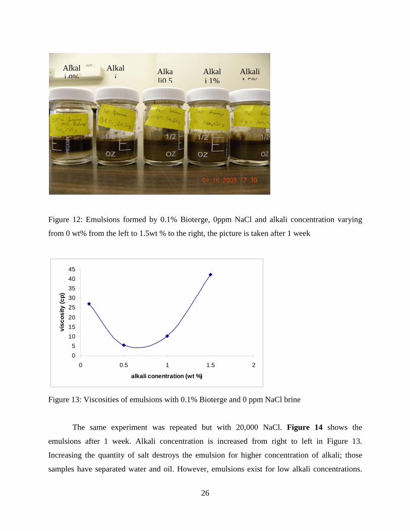
0 to 1.5 wt % (from left to right). There is emulsion in all the samples. Figure 12 shows the same

samples after 1 week. The leftmost sample which did not contain any alkali showed a fast

separation of the oil and water. As the alkali concentration is increased, stable emulsions form

which do not separate out within at least a week. The total surfactant in the system (surfactant +

soap) increases with the addition of alkali which may account for stable emulsion formation.

Figure 13 plots the viscosity of the lower emulsion phase. The viscosities are much lower than

the oil viscosity and did not show any shear rate dependence. The minimum emulsion viscosity

is obtained for the sample with 0.5 wt % alkali.

Figure 11: Emulsions formed by 0.1% Bioterge, 0 ppm NaCl and alkali concentration varying

from 0 wt% from the left to 1.5 wt % to the right, the picture is taken immediately after mixing

Alkali

Alkali 0 1%

Alkali 0.5%

Alkali1%

Alkali 1.5%

26

Figure 12: Emulsions formed by 0.1% Bioterge, 0ppm NaCl and alkali concentration varying

from 0 wt% from the left to 1.5wt % to the right, the picture is taken after 1 week

05

101520

2530354045

0 0.5 1 1.5 2

alkali conentration (wt %)

visc

osity

(cp)

Figure 13: Viscosities of emulsions with 0.1% Bioterge and 0 ppm NaCl brine

The same experiment was repeated but with 20,000 NaCl. Figure 14 shows the

emulsions after 1 week. Alkali concentration is increased from right to left in Figure 13.

Increasing the quantity of salt destroys the emulsion for higher concentration of alkali; those

samples have separated water and oil. However, emulsions exist for low alkali concentrations.

Alkali 0%

Alkali

Alkali0.5

Alkali 1%

Alkali 1 5%

27

The viscosities of these emulsions (bottom phase) are displayed in the figure; 0.1 wt % alkali

gave the lowest viscosity of 8.9 cp.

Figure 14: Emulsions formed by 0.1% Bioterge, 20,000ppm NaCl and alkali concentration

varying from 0 wt% from the right to 1.5wt % to the left, the picture is taken after 1 week

b) Tergitol 15-S-20 surfactant

This is a nonionic surfactant. The mixtures with WOR of 9 show a behavior similar to

that shown in Figure 12 for the Bioterge surfactant. Oil and water separate out for the sample

with 0 % alkali. The samples with 0.1 to 1.5 wt% alkali formed oil-in-water emulsions. The

viscosity of these emulsions was shear-rate dependent. Figure 15 shows the viscosity of these

emulsions as a function of the shear rate. The solution with 0.5 % alkali gave the lowest viscosity

of about 7 cp. The emulsion viscosity was high (above 100 cp) for samples with greater than 1

wt% alkali.

These experimented were repeated with 20,000 ppm NaCl brine. Emulsions were seen at

the low alkali concentration (0 wt% and 0.1wt% alkali), but not at higher alkali concentration.

The sample without any alkali gave the lowest emulsion viscosity of 1.5cp.

Alkali

Alkali 0.5%

Alkali 1%

Alkali 1.5%

Alkali 0%

28

Figure 15: Viscosity variation of emulsions with 0.1% 15-S-20, 0ppm NaCl and varying alkali

concentration

Figure 16: Emulsions formed by 0.1% TDA-30EO, 20,000ppm NaCl and alkali concentration

varying from 0 wt % from left to 1.5 wt % to the right, the picture is taken after 1 week

c) TDA-30EO surfactant

Alkali 0.5%

Alkali 1%

Alkali 1.5%

Alkali 0.1%

Alkali 0%

29

TDA-30EO is a nonionic surfactant and is even more hydrophilic than Tergitol 15-S-20.

Figure 13 shows the emulsion behavior with 20,000 ppm NaCl after 1 week of equilibration.

Emulsification was observed in samples with < 1 wt% alkali. The sample with 0.5 wt% alkali

had a viscosity of 2.7 cp. TDA 30EO surfactant with 0.5 wt% alkali was chosen for further

studies.

Figure 17: Emulsions with 0.1 wt% TDA-30EO, 0.5 wt% alkali and 20,000 ppm NaCl with

WOR varying from 9:1 (left) to 7:3 (right).

WOR 7:3

WOR 7.5:2.5

WOR 8:2

WOR 8.5:1.5

WOR 9:1

WOR 7:3

WOR 7:3

WOR 8.5:1.5

30

Figure 18: Emulsions with 0.1 wt% TDA-30EO, 0.5 wt% alkali and 0 ppm NaCl with lowest

WOR of 7:3 at the left. It is still an O/W emulsion with a viscosity of a few hundred centipoises

The preliminary surfactant screening was done at a high WOR of 9:1. In this part of the

study, the surfactant was kept constant (0.1 wt% TDA-30EO), but the WOR was varied. Figure

17 shows the emulsion behavior when the WOR was decreased from 9:1 to 7:3 with 20,000 ppm

NaCl brine. The O/W emulsion was observed at high WORs; the emulsion changed to high-

viscosity water-in-oil (W/O) emulsion at lower WOR (right two samples). The W/O emulsion in

the right most sample had a viscosity of 21,130 cp (twice the viscosity of the crude oil) at 0.6 s-1

shear rate. As the WOR decreases, more soap is generated which makes the soap-surfactant

mixture more hydrophobic and destabilizes the O/W emulsions.

Emulsion studies with TDA-30EO surfactant

Figure 18 shows the emulsion behavior with WOR variation for 0 ppm NaCl. All the

samples showed O/W emulsions. At the lowest WOR (at the left) an O/W emulsion was present

with a viscosity of a few hundred centipoises at low shear rates. The viscosity dependence on the

shear rate is shown in Figure 19.

Figure 19: Viscosity of the emulsion at WOR = 7:3

31

From the above two tests it was concluded that the emulsion behavior depends on salinity

of the brine as well as the WOR. A salinity scan was performed at a WOR of 7:3 to determine

the salinity at which a transition takes place from O/W emulsions to W/O emulsions. Figure 20

shows the state of emulsions with increasing salinity from left to right. At low salinities, O/W

emulsions appear at the bottom with their light brown color. As the salinity is increased to about

7500ppm the O/W emulsions changed to W/O emulsions with dark brown phases appearing at

the top of the aqueous phase. As the salinity increases, the electrostatic repulsion between oil

drops decreases and O/W emulsions are unstable.

Figure 20: Emulsions with 0.1 wt% TDA 30EO, 0.5 wt% alkali and salinity increasing from 0

ppm (left) to 10,000 ppm (right)

The surfactant phase behavior studies showed that emulsion behavior depends on salinity,

alkali concentration and WOR. It was possible to form O/W emulsions under lower salinity and

higher WOR. Sand pack floods were conducted to see the effect of alkali-surfactant solutions on

oil recovery.

32

1D Sand Pack Floods of the Viscous Oil

Sand pack floods were performed in order to determine the effectiveness of the alkali

surfactant polymer formulations in a 1D flooding system. The flood started with the water

injection for about 3 PV followed by an alkali-surfactant-polymer slug of about 0.5 PV. This

slug was followed by the polymer slug for about 2PV. In order to minimize the use of polymer,

the polymer concentration was gradually reduced and finally only water was injected for about

half a pore volume. A partially hydrolyzed polyacrylamide (HPAM) provided by SNF is used in

all the cases. Table 3 shows the injection scheme. Surfactant and alkali concentrations were

chosen on the basis of the phase behavior experiments. Polymer concentration was chosen such

that the ASP slug mobility would be lower than that of the oil bank that forms due to the

mobilization of the residual oil.

Table 5: Injection scheme

Fluid Injected PV injected Viscosity

20,000 ppm brine 3 PV 1 cp

ASP slug

0.5PV 537.03 cp

(shear rate = 1 s-1) 0.4 wt% surfactant

20,000 ppm brine, 1.5 wt% alkali, 0.48 wt% polymer

Polymer slug 1PV

613.74 cp

(shear rate = 1 s-1) 20,000 ppm brine, 0.48 wt% polymer

Polymer slug 0.5PV

329.51 cp


Polymer slug 0.5PV

158.71 cp


0.5PV 1 cp

20,000 ppm brine

As shown in Table 5, the polymer slug does not contain any alkali. This is done to

introduce a negative gradient in alkali concentration. The negative gradient in the alkali

concentration ensures that the surfactant flood passes through a Type III region where the IFTs

are the lowest and ends in Type I region for minimum surfactant retention. The viscosity of

33

polymer slug is reduced by approximately half in every slug. It is to be noted that the original

high viscosity polymer slug was injected for about 1 PV and the tapered slugs are subsequently

injected for around 0.5 PV. Tapering the polymer slug in stages is necessary to minimize the

effect of adverse mobility ratio. The tapering also reduces the amount of polymer and thus the

cost. A secondary polymer flood was also conducted in the sand pack. This polymer slug had the

same composition as the chase polymer slug in the ASP flooding (i.e., 0.48 wt% in 20,000 ppm

brine). The flow rate was kept the same (0.02 ml/min).

Figure 21 shows the cumulative oil recovery and the oil cut. Water broke through the

pack at about 0.27 PV injection. Oil continued to be recovered after water breakthrough. The

recovery at 3 PV injection was about 0.61 PV. The oil cut was almost steady at about 0.05

between 1.5 and 3 PV injection. ASP slug was injected after the waterflood.

0

0.2

0.4

0.6

0.8

1

1.2

0 0.5 1 1.5 2 2.5 3 3.5

Cum

ulat

ive

Oil

Reco

vere

d (P

V)/

Oil

Cut

Fluids Injected (PV)

Waterflood Oil Recovery

Cumulative Oil Recovery Oil Cut

Figure 21: Cumulative oil recovery and oil cut for waterflood

Figure 22 shows the cumulative oil recovery and oil cut for the alkali surfactant polymer

flood. The size of the ASP slug was about 0.38 PV. The flood responded to the ASP slug in

about 0.5 PV. Oil cut increased to about 0.6 and then decreased. High oil cut persisted for

34

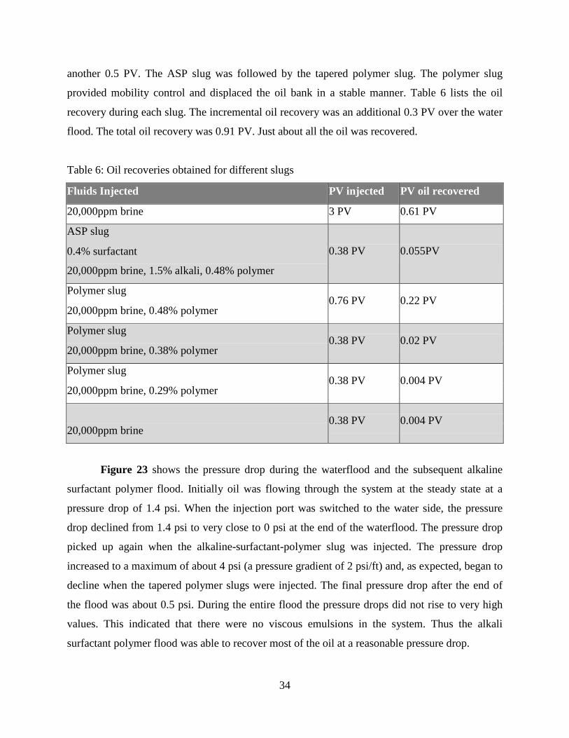
another 0.5 PV. The ASP slug was followed by the tapered polymer slug. The polymer slug

provided mobility control and displaced the oil bank in a stable manner. Table 6 lists the oil

recovery during each slug. The incremental oil recovery was an additional 0.3 PV over the water

flood. The total oil recovery was 0.91 PV. Just about all the oil was recovered.

Table 6: Oil recoveries obtained for different slugs

Fluids Injected PV injected PV oil recovered

20,000ppm brine 3 PV 0.61 PV

ASP slug

0.38 PV 0.055PV 0.4% surfactant

20,000ppm brine, 1.5% alkali, 0.48% polymer

Polymer slug 0.76 PV 0.22 PV

20,000ppm brine, 0.48% polymer





0.38 PV 0.004 PV

20,000ppm brine

Figure 23 shows the pressure drop during the waterflood and the subsequent alkaline

surfactant polymer flood. Initially oil was flowing through the system at the steady state at a

pressure drop of 1.4 psi. When the injection port was switched to the water side, the pressure

drop declined from 1.4 psi to very close to 0 psi at the end of the waterflood. The pressure drop

picked up again when the alkaline-surfactant-polymer slug was injected. The pressure drop

increased to a maximum of about 4 psi (a pressure gradient of 2 psi/ft) and, as expected, began to

decline when the tapered polymer slugs were injected. The final pressure drop after the end of

the flood was about 0.5 psi. During the entire flood the pressure drops did not rise to very high

values. This indicated that there were no viscous emulsions in the system. Thus the alkali

surfactant polymer flood was able to recover most of the oil at a reasonable pressure drop.

35

0

0.2

0.4

0.6

0.8

1

3 3.5 4 4.5 5 5.5 6

Cum

ulat

ive

Oil

Reco

vere

d (P

V)/

Oil

Cut


ASP Oil Recovery

Series1 Series2

ASP Polymer0.48%

Tapered Polymerslugs

Figure 22: Cumulative oil recovery and oil cut for the ASP flood

Figure 23: Pressure drop during waterflood and alkaline surfactant polymer flood

36

Figure 24 shows the oil recovery and oil cut in a secondary polymer flood in the sand

pack. In this case, porosity and permeability were 43.7% and 26 md. The initial oil saturation

was 87%. Secondary polymerflood was conducted with 0.48 wt% polymer in a 20,000 ppm

brine. 1.29 PV of the polymeric solution was injected followed by 0.38 PV of brine. Polymeric

solution broke through at about 0.6 PV injection, compared to 0.3 PV for brine injection. The oil

recovery was about 0.78 PV by 1 PV injection. Very little oil was recovered beyond 1 PV

injection. This recovery is much higher than 0.61 PV recovery due to water flood in 3 PV

injection. Figure 25 shows the pressure drop during the secondary polymer flood. It increases

from the intial pressdure drop of 2.5 psi during the initial oil flow to about 4.5 psi steadily as the

polymer comes into the core. Thus the mobility of the polymer slug is smaller than that of the

original oil by a factor of (2.5/4.5). This flood is stable. When the brine is injected following the

the polymer slug, the pressure drop decreases steadily to a final value of about 0.5 psi. These

floods show that a secondary polymer flood is stable and can displace a large portion of the oil.

But it does leave behind a residual oil saturation due to capillary trapping. The ASP flood can

displace all the oil out leaving behind almost no residual.

Figure 24: Cumulative oil recovery and oil cut for the secondary polymer flood

37

Figure 25: Pressure drop for the secondary polymer flood

38

1D Sand Pack Floods of the Heavy Oil

a) Injection of 20,000 ppm brine followed by alkaline surfactant injection at 0.018 ml/min

Both the brine flood and the alkaline surfactant flood are conducted here with 20,000

ppm NaCl brine. The injection rate was chosen to be 0.018 ml/min, which corresponds to 1 ft/D

superficial velocity. Figure 26 shows the cumulative oil recovery and the pressure profile for the

brine and surfactant floods at a relatively low rate. Brine injection was continued for 3.65 PV.

The water flood recovery is 0.38 PV, which is low, compared to the waterflood recovery of low

viscosity oils. The pressure drop reaches a maximum of 44 psi during the waterflood and then

decreases. The initial increase in the pressure drop indicates some compressibility in the system,

perhaps due to unconsolidated sand pack and viscous oil. The pressure drop would have been 88

psi for oil flowing at this flow rate if the permeability is 20 D. The flood is marked by the early

breakthrough (<0.1 PV) of the water phase. The pressure drop falls as the water flows through

the fingers; subsequent recovery is due to incremental growth of the water finger along the sides

of the fingers. The alkaline-surfactant (AS) slug injection starts at 3.65 PV and ends at 8 PV.

During the injection of AS slug, the pressure drop increases to 30 psi and then decreases. At the

time of high pressure, significant amounts of additional oil are mobilized and emulsions are

generated in situ. The oil recovery increases to 0.75 PV at the end of the AS flood, an

incremental oil recovery of 0.37 PV due to alkaline surfactant injection.

00.10.20.30.40.50.60.70.8

0 1 2 3 4 5 6 7 8

fluids injected (PV)

oil r

ecov

ery

(PV)

0

10

20

30

40

50

pres

sure

dro

p (p

si)

20,000ppm brine flood, 0.018ml/min

surfactant (0.1% TDA, 0.5%alkali), 20,000ppm NaCl flood, 0.018ml/min

pressure drop

Emulsion viscosity >30,000cp

Brine flood Surfactant flood

39

Figure 26: Oil recovery and pressure drop for 20,000 ppm brine flood at 0.018 ml/min followed

by the surfactant (0.1 wt% TDA, 0.5 wt% alkali and 20,000 ppm NaCl) injection.

Figure 27: Oil cut and pressure drop for 20,000 ppm brine flood and alkaline surfactant flood

Figure 27 plots the fractional flow of oil, W/O emulsion phase and O/W emulsion phase

during this flood. The pressure drop is also shown. During the brine flood, only water and oil are

produced. Oil cut decreases as the flood proceeds. After the alkaline surfactant injection starts,

for about 1.35 PV only water and oil are produced, but the oil cut increases. Then the effluent

changes to W/O emulsion and excess water, at about 5 PV injected. At about 6.6 PV injected, the

effluent changes to O/W emulsion. Peaks in oil or W/O emulsion cut follow the peaks in

pressure drop. Both oil and W/O emulsion are viscous. W/O emulsion viscosity reaches higher

than 30,000 cp. This is due to the oil-water emulsions forming in the porous media. The pressure

drop is very low at the end of the flood when only low viscosity O/W emulsion is observed at the

outlet.

The emulsions were broken to separate the oil and water components and the component

oil cut was measured. Figure 28 plots the surface tension of the aqueous phase and the oil

00.10.20.30.40.50.60.70.80.9

1

0 1 2 3 4 5 6 7 8


oil/e

mul

sion

cut

' fo

'

0

10

20

30

40

50

60

pres

sure

dro

p (p

si)

oil cut W/O emulsion cut O/W emulsion cut pressure drop

brine flood surfactant flood

W/O highviscosity emulsion

O/W lowviscosity emulsion

oil

40

concentration in effluent phases. The surface tension of the produced aqueous phase was 53

dynes/cm during the waterflood. The surface tension of the injected brine was measured to be 72

dynes/cm; hence it is evident that the produced brine had some dissolved component from the

oil, which was responsible for lowering its surface tension. The surface tension of the produced

fluid decreased further when the surfactant was produced at the outlet. However the graph shows

that it took almost a pore volume for the surfactant to break through. This is because the

surfactant is reacting with the oil inside the porous medium and forming emulsions rather than

just flowing through the viscous fingers. The concentration of the oil component in the oil phase

shows a distinct decrease, once W/O emulsions are formed. These W/O emulsions have a lot of

water emulsified in them. After about 6.6 PV only O/W emulsion is produced. There was a very

small concentration of oil in this emulsion phase. It is suspected that alkaline surfactant flow in

the water fingers generates O/W emulsions at the surface of the fingers. Oil is drawn into the

fingers while the finger width grows. As O/W emulsion flows through porous media, oil

accumulates and transforms to W/O emulsions and thus the effluent is W/O emulsion soon after

alkaline surfactant injection. Towards the end of the experiment, little oil is mobile; thus O/W

emulsion is produced with low oil content and pressure drop.

0

10

20

30

40

50

60

0 1 2 3 4 5 6 7 8


surf

ace

tens

ion

(dyn

es/c

m)

0

0.2

0.4

0.6

0.8

1

1.2co

ncen

trat

ion

of

oil C

o (m

l/ml)

surface tension, brine floodsurface tension, surfactant flood concentration of oil in oil phase Cooconcentration of oil in the aqueous phase Cow

Brine flood surfactant flood

oil W/Oemulsion

O/W emulsion

Figure 28: Surface tension and concentration of the oil component

41

b) Injection of 8900 ppm brine followed by alkali surfactant slug at 0.018 ml/min

Figure 29 shows the oil recovery and pressure drop obtained by injecting 8900 ppm brine

followed by alkaline surfactant injection at the same low flow rate. This experiment is identical

to the last experiment, except that the brine and alkaline surfactant salinity is reduced to 8900

ppm. 2.2 PV of brine injection produced about 0.26 PV of oil; the subsequent alkaline surfactant

flood produced 0.42 PV of oil giving a total of 0.68 PV of oil. High viscosities W/O emulsions

were observed at the outlet as the oil cut increased after alkaline surfactant injection.

00.10.20.30.40.50.60.70.8

0 1 2 3 4fluids injcted (PV)

oil r

ecov

ery

(PV)

0

0.025

0.05

0.075

0.1

oil c

ut (P

V)8900ppm brine flood, 0.018ml/min

surfactant (0.1% TDA, 0.5% alkali), 8900ppm NaCl flood, 0.018ml/min

Oil cut

Brine Flood Surfactant Flood

Emulsion viscosity>30,000cp

Figure 29: Oil recovery and pressure drop for 8900 ppm brine flood followed by the surfactant

(0.1 wt% TDA, 0.5 wt% alkali and 8900 ppm NaCl) injection

c) Injection of deionized (DI) water followed by alkali surfactant slug at 0.018 ml/min

Figure 30 shows the oil recovery and the pressure drop when DI water was injected

followed by alkaline surfactant injection. This flood was performed at the same flow rate of

0.018 ml/min as the last two experiments, the only difference being the salinity. The oil recovery

is 0.37 PV of oil in about 3 PV water injection; this recovery is very similar to the first

experiment. The pressure drop maximum was about 50 psi, which is also similar to the first

experiment. The oil recovery during the alkaline surfactant flood was about 0.19 PV, not as high

42

as the earlier experiments. This time low viscosity O/W emulsions were observed at the outlet.

These emulsions can flow easily at low pressure drops but do not contain as much oil as W/O

emulsions. The pressure drop stayed below 10 psi. The possible mechanism of oil recovery is the

entrainment of oil from the sides of the fingers into the flowing aqueous solution, but lack of

conversion to a W/O emulsion. May be the low salinity stabilized the oil emulsion droplets and

prevented them from coalescing.

0

0.1

0.2

0.3

0.4

0.5

0.6

0 2 4 6fluids injected (PV)

oil r

ecov

ery

(PV)

0

10

20

30

40

50

60

pres

sure

dro

p (p

si)

0ppm water flood, 0.018ml/minsurfactant (0.1% TDA 0.5% alkali) 0ppm NaCl flood, 0.018ml/minpressure drop

DI water flood Surfactant flood

7-20 cp

Figure 30: Oil recovery and pressure drop for DI water flood followed by the surfactant (0.1 wt%

TDA, 0.5 wt% alkali, and 0 ppm NaCl water) injection

d) Injection of 20,000 ppm brine followed by the alkali-surfactant slug at 0.1ml/min

This experiment was conducted with the same fluids as in the first experiment (20,000

ppm brine), but the flow rate was about 5.5 times faster. Figure 30 shows the cumulative oil

recovery and the pressure profile for the brine and alkaline surfactant floods at this relatively

high rate. Brine injection was continued for 3.65 PV. The water flood recovery is 0.225 PV,

which is quite low, compared to waterflood recovery of first experiment (0.38 PV). The

maximum pressure drop during waterflood decreases from 44 psi (in the first experiment) to 30

psi (in this experiment), even though the flow rate was 5.5 times higher. The displacement front

during the high flow rate water flood is more unstable which is evident by the faster water

breakthrough. The oil left behind at the end of water flood is larger in this case compared with

43

the first experiment. The alkaline surfactant (AS) injection starts at 3.65 PV and ends at 5 PV.

During the injection of AS slug, the pressure drop increases to 110 psi and then decreases. At the

time of high pressure, significant amounts of additional oil are mobilized and emulsions are

generated in situ. The oil recovery increases to 0.47 PV at the end of the AS flood. The

incremental oil recovery is 0.25 PV at this high flow rate compared to 0.38 PV for the first

experiment. The generation of viscous W/O emulsion is verified by the viscosity observed at the

outlet. The emulsions had a viscosity ranging from 17,000 – 21,000 cp. Oil is possibly mobilized

by emulsification. The mobilized emulsion fills the waterflood fingers to give high pressure

drops.

A comparison of all the floods (Figure 32) throws some light on the effect of salinity and

flow rate. All the waterfloods at the low injection rate have about the same oil recovery

irrespective of the salinity of the water. But the increase in flow rate decreases oil recovery by

waterflood. The oil recovery due to alkaline surfactant floods varies from 0.19 to 0.42 PV. The

high recoveries are associated with higher salt concentrations, but the pressure drop is also

higher in these cases during alkaline surfactant floods.

Figure 31: Oil recovery and pressure drop for 20,000 ppm brine flood followed by the surfactant

(0.1 wt% TDA, 0.5 wt% alkali and 20,000 ppm NaCl brine) injection

More investigation is needed to understand these displacements. It is hypothesized that

oil-in-water emulsions form in all cases in situ at the surface of the water fingers. In the case of

44

high salinity, the oil droplets accumulate as the flow through the porous medium and form water-

in-oil emulsions. With deionized water, oil-in-water emulsions stay stable and avoid forming

water-in-oil emulsions. A mechanistic understanding must be developed to model and upscale

these displacements.

0

0.1

0.2

0.3

0.4

0.5

0.6

0.7

0.8

0 1 2 3 4 5 6 7 8 9


oil r

ecov

ery

(PV)

20000ppm salinity high flow rate 0ppm brine 8900ppm brine 20000ppm brine

Figure 32: Comparison of floods

2D Floods for Viscous Oil

Figure 33: Displacement of the viscous oil by the ASP slug in the quarter 5-spot model

45

Figure 33 shows the displacement front of the ASP slug in a 2D quarter 5-spot following

a waterflood. It shows that the displacement front is stable. No viscous fingers are visible at the

displacement front. Thus the ASP formulation can displace the oil in the reservoir in a stable

mode.

2D Floods for Heavy Oil

This flood was conducted in sand pack # 1. The water flood with 20,000 ppm NaCl brine

is followed by the AS flood at the same salinity. Figure 34 shows the oil recovery and the oil cut

for this flood. The oil recovery during the brine flood is about 35% of OOIP. Breakthrough

occurred at about 0.04 PV of brine injection. The low value of the breakthrough PV gives an

indication that the displacement process is unstable and that viscous fingering dominates the

flow behavior. Significant amount of oil is recovered after breakthrough which may be due to the

cocurrent imbibition of water from the fingers into bypassed regions. Our previous study had

indicated that the post-breakthrough oil recovery in a linear core was proportional to the square

root of the time. The oil recovery had a significant jump soon after the AS injection started. This

increase in oil cut is due to the formation of emulsions in the porous medium which pushes out

oil from the fingers and from the surrounding unswept zone. The initial production of oil during

the AS flood was followed by the production of emulsions. These emulsions were then broken

down to measure the oil recovery. The oil cut also increased to almost 1 for a short duration. The

incremental oil recovery due to the AS flood was about 18% of OOIP.

a) Injection of 20,000 ppm brine followed by the AS flood at the same salinity

46

Figure 34: Oil recovery and oil cut for 20,000 ppm brine flood followed by alkaline-surfactant

injection with 20,000 ppm NaCl brine

Figure 35: Pressure drop for 20,000 ppm brine flood followed by alkali-surfactant injection with

20,000 ppm NaCl brine

0

0.2

0.4

0.6

0.8

1

1.2

0

10

20

30

40

50

60

0 1 2 3 4 5

Cum

Oil

Rec

(%)


Oil Recovery

Oil Cut

Brine floodAlkali Surfactantflood

0

10

20

30

40

50

60

0 1 2 3 4 5

Pres

sure

dro

p (p

si)

Fluids injected (PV)

Pressure Drop Brine Flood Alkaline surfactant

flood

47

Figure 35 shows the pressure drop for the flood. The flood was started from an initial

condition of no flow (0 psi pressure drop). The pressure drop increased from 0 to 50 psi as the

injected brine fingers push out the oil. After the brine breakthrough, oil cut and pressure drop fell

sharply to about 2 psi. Injection of the AS solution mobilized oil and increased the pressure drop.

The pressure drop rose to 15 psi and then dropped to about 1 psi. The cumulative oil recovery

showed a big jump of around 15% of OOIP during the pressure spike. After this spike, oil cut

dropped once again. Most of the extra oil was already produced. Oil in water low viscosity

emulsions were now observed at the outlet. These emulsions have a low oil concentration (< 2%

by volume) which is also evident by the lower increments in the oil recovery curve. They also

had a low viscosity (< 10 cp) and this is the reason for the fall in the pressure drop.

Figure 36 shows the state of the 2D cell after the waterflood. The injection port was at

the top corner; the production port was at the bottom corner. The lighter region represents water

invaded pores on the top of the model. Distinct viscous fingers were not observed possibly

because the oil adhered to the plastic plate and the pack was truly three-dimensional. However,

patches of dark (oil) and light (water) regions can be seen throughout the sand pack. This picture

gives an indication that the water fingers formed in the entire region and a large amount of oil

was unswept.

48

Figure 36: State of the 2D cell (sand pack # 1) after the waterflood

AS injection increased the oil recovery beyond that of the waterflood. A distinct finger

was observed during alkaline-surfactant flood, as shown in Figure 37. The AS solution removed

the oil from the top plastic plate of the cell where the finger went through. The AS solution

mobilized the trapped oil within the fingers and the oil adjacent to the fingers (at least near the

injection section of the pack). The mobilized oil can react with the AS solution to form high

viscosity W/O emulsions at conditions of low WOR. The high viscosity of the emulsions can aid

in the effective displacement of oil. We observed patches of water filled pore getting resaturated

with oil. The pore-scale water fingers disappeared and the AS solution got a chance to flow

laterally and thus improve the sweep efficiency of the process. Thus the AS solution, in addition

to improving the displacement efficiency by mobilizing the trapped oil, also was helpful in

improving the sweep efficiency of the flood. Finally, AS solution itself formed its own large

fingers due to its low viscosity and produced low viscosity O/W emulsions by entrainment of

small volumes of oil from the sides of the fingers.

Figure 37: State of the 2D cell (sand pack # 1) during the AS flood

49

The oil recovery increased from 35% after the waterflood to 53% after the AS flood.

Further improvement in the process may be possible by changing salinity of the AS flood. These

parameters are addressed in the following experiments.

This flood was conducted in sand pack # 2. Our previous experiments had shown that the

emulsion behavior changes at 5,000 ppm salinity from O/W (at lower salinities) to W/O (at

higher salinities). We wanted to look for the effect of this change in emulsion behavior on the oil

recovery. We used the opaque steel model for this flood because some cracks were developed in

our transparent model during repacking of the sand. This model had a lower permeability and

porosity due to the wet packing and the applied overburden pressure. A 2,000 ppm brine was

injected for 2.5 PV followed by the AS solution at the same salinity. Figure 38 shows oil

recovery and oil cut for this flood.

b) Injection of 2,000 ppm brine followed by the AS flood at the same salinity

This flood had a different starting condition than the previous flood. Before starting the

water flood, oil was injected into the pack at a constant flow rate of 0.1 ml/min until a steady

pressure was reached. The water pump was pressurized to the same pressure and the injection

was then switched from oil to water. This is the reason why the pressure drop in the Figure 39

starts from a high value of 311 psi (rather than from 0 psi as in the previous flood). The pressure

drop falls quickly as the injected water fingers through the oil and the recovery rates decrease.

50

Figure 38: Oil recovery and oil cut for 2,000 ppm brine flood followed by alkali-surfactant

injection with 2,000 ppm NaCl brine

0

40

80

120

160

200

240

280

320

0 0.5 1 1.5 2 2.5

Pres

sure

dro

p (p

si)


Waterflood pressure drop

Figure 39: Waterflood pressure drop for 2,000 ppm brine flood

The oil recovery from the waterflood reached to about 33% OOIP and the breakthrough

occurred at 0.074 PV. The cumulative oil recovery is almost identical to the previous flood

although the breakthrough recovery is higher. The difference may arise from the differences in

the starting condition, porosity, and heterogeneity of the packs. The oil recovery after the water

51

breakthrough is again very significant. The oil cut plateaus at about 5% for a long time. The oil

cut increases again on injection of the AS solution to a level of 40% after which it declines

slowly to a plateau of about 10%. The increase in oil recovery due to AS injection is more

gradual in this flood than the first flood. The extra oil was recovered as a separate phase for

about a PV (from 2.8 to 3.8 PV). After this time the O/W emulsions were produced at the outlet.

These emulsions were broken down (outside the sand pack) to measure their oil content. Finally,

about 57% of OOIP could be recovered by this flood; the last 24% OOIP can be ascribed to the

AS flood. Oil was still coming out when the flood was stopped at 4.5 PV injection.

The pressure drop (Figure 40) during the AS flood follows the same trend as the oil

recovery. The increase in oil recovery is accompanied by an increase in pressure drop. The

pressure drop increased to 25 psi which is higher than that in the previous flood. The difference

may be due to the lower permeability of the sand pack # 2. The repetition of the first flood in this

2D cell will be undertaken in the future to get comparable results.

0

5

10

15

20

25

30

2 2.5 3 3.5 4 4.5 5

Pres

sure

dro

p (p

si)


AS flood pressure drop

Figure 40: 2,000 ppm NaCl AS flood pressure drop following 2,000 ppm brine flood

This flood was conducted in sand pack # 2. After conducting the two floods at constant

brine salinity, we wanted to look into the effect of introducing a salinity gradient in our floods.

The brine injection was performed at a higher salinity of 20,000 ppm brine and the AS solution

c) Injection of 20,000 ppm brine followed by the AS flood at 0ppm salinity

52

was injected at 0 ppm brine. In our previous 1D floods, a strong dependence of the oil recovery

on salinity was observed.

0

0.2

0.4

0.6

0.8

1

1.2

0

10

20

30

40

50

60

0 1 2 3 4 5 6

Oil

Cut

Cum

Oil

Rec

(%)


Oil Recovery

Oil Cut

Brine floodAlkali Surfactantflood

Figure 41: Oil recovery and oil cut for 20,000 ppm brine flood followed by alkaline-surfactant

injection at 0 ppm NaCl brine

Figure 41 shows the oil recovery and the oil cut during the flood. The waterflood

recovery is same as in the second flood due to the same properties of the pack. The pressure drop

profile was also identical for the same reason and hence is not plotted. The oil recovery during

the AS flood did not show any appreciable jump and the oil cuts remained low (under 10%)

during the entire course of the flood. This behavior indicates that the emulsion behavior at least

near the outlet is almost entirely controlled by the AS brine and the mixing had a negligible

effect on oil recovery. The pressure drop (Figure 42) did however show an increase to about 13

psi. Further data could not be obtained due to the malfunction of the recording instrument. Hence

we are not yet sure how exactly would the pressure drop respond later in the experiment. The

final oil recovery was only about 51% OOIP which is much lower than the second flood.

53

0

2

4

6

8

10

12

14

2.3 2.4 2.5 2.6 2.7 2.8 2.9

Pres

sure

dro

p (p

si)


AS flood pressure drop

Figure 42: 0 ppm NaCl AS flood pressure drop following 20,000 ppm brine flood

Figure 43 compares the cumulative oil recovery in these three floods. The brine flood oil

recovery was independent of the brine salinity. However, there was a significant change in the

AS flood oil recovery with the salinity of the injection solution. Alkaline-surfactant flood at the

high salinity flood produced a large increase in the oil cut for a short time followed by very low

oil cut. As the salinity of the AS solution is decreased, the additional oil recovery becomes more

gradual. The difference in this behavior arises due to the difference in the emulsion behavior

inside the pack. The emulsion obtained at high salinities had a higher viscosity. At lower

salinities, the low viscosities of the emulsions resulted in lower oil cuts and lower pressure drops.

54

0

10

20

30

40

50

60

0 1 2 3 4 5 6

Cum

Oil

Rec

(%)


2,000 ppm salinity brine and AS flood

20,000 ppm brine flood 0 ppm AS flood

20000 ppm salinity brine and AS flood

Brine flood Alkali Surfactantflood

Figure 43: Comparison of floods at different salinities

55

Micromodel Studies

This section has been divided into three parts: secondary flooding, tertiary flooding,

simulation and image analysis. In the secondary flooding section, we discuss the case of water or

polymer injection into the micromodel saturated with oils of different viscosity. In the tertiary

flooding section, we describe the effect of injection of alkali surfactant solution on the already

water flooded micromodel. In the simulation and image analysis section, we discuss simulation

of DLA type fractals and fractal analysis of the images gathered during the experiments.

Secondary Floods

Viscosity ratio, µr = 1 (6 cP Oil Displaced by 6 cP Glycerol-Water Solution)

Figure 44: Water saturation front for unit viscosity ratio displacement after the injection of 7µl

and 25 µl; water was injected at the top left corner and the producer was at the bottom right

corner

Experiment 6 was conducted just to illustrate stable flow through the micromodel. In this

experiment, the micro-model was first saturated with a light reservoir oil of viscosity about 6 cP.

The oil was then displaced by a glycerol water solution of about the same viscosity. The

viscosity ratio (µr) between the displaced and the displacing fluids was one. The water

distribution is shown in Figure 44 at two different times. As expected the displacement front is

very stable and moves through the micromodel from the left top corner to the bottom right

1

1

56

corner. Viscous fingering or any kind of instability due to the non-homogeneity in the micro-

model was not observed.

Figure 45: Fingers during water flood with µr = 10,000; 80 µl injected

Viscosity ratio, µr = 10,000 (10000 cP Oil Displaced by 1 cP Brine)

In Experiment 1, 20,000 ppm NaCl brine was injected into a micro-model that was

saturated with a 10,000 cp oil. Figure 45 shows the fingers formed after 80 µl of brine was

injected into the system. The fingering is at the pore scale. Side branches form during the growth

of the finger, but side branches do not grow much. Water takes the shortest path (path of least

resistance) from the inlet to the exit channel. A large portion of the micromodel remains unswept

and hence, the recovery is poor. The finger has a structure like the ones modeled by diffusion

limited aggregation (DLA). The water injection was stopped after about 2.1 ml of water was

injected. Figure 46 shows the final picture of the micromodel at the end of the water flood. A

lot of water resides in the side branches of the finger which do not contribute to flow. Only the

flowing fraction (a small part of the water saturation) contributes to the flow and hence the water

relative permeability tends to be lower than those for light oil displacements in the same porous

medium. The oil in pores next to the side branches of the water is also immobile. Therefore the

oil relative permeability is lower than those of the light oils at similar saturations (Wang et al.,

2006). The fractal pattern formed in the process of viscous fingering justifies the observed

decrease in both oil and water relative permeability in the case of viscous oils.

1 cm

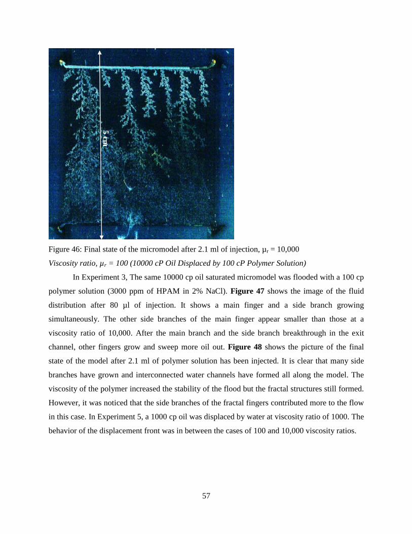
57

Figure 46: Final state of the micromodel after 2.1 ml of injection, µr = 10,000

Viscosity ratio, µr = 100 (10000 cP Oil Displaced by 100 cP Polymer Solution)

In Experiment 3, The same 10000 cp oil saturated micromodel was flooded with a 100 cp

polymer solution (3000 ppm of HPAM in 2% NaCl). Figure 47 shows the image of the fluid

distribution after 80 µl of injection. It shows a main finger and a side branch growing

simultaneously. The other side branches of the main finger appear smaller than those at a

viscosity ratio of 10,000. After the main branch and the side branch breakthrough in the exit

channel, other fingers grow and sweep more oil out. Figure 48 shows the picture of the final

state of the model after 2.1 ml of polymer solution has been injected. It is clear that many side

branches have grown and interconnected water channels have formed all along the model. The

viscosity of the polymer increased the stability of the flood but the fractal structures still formed.

However, it was noticed that the side branches of the fractal fingers contributed more to the flow

in this case. In Experiment 5, a 1000 cp oil was displaced by water at viscosity ratio of 1000. The

behavior of the displacement front was in between the cases of 100 and 10,000 viscosity ratios.

5 cm

1

58

Figure 47. Fingers during polymer flood with µr = 100, 180 µl injected

Figure 48. Final state of the micromodel after 2.1 ml of injection, µr = 100

Tertiary Floods

Alkali Surfactant Flooding in the Water Flooded Micromodel

An alkali surfactant mixture was prepared as per the composition shown in Table 6. This

composition produces an oil-in-water emulsion when mixed in 1:9 ratio of oil to brine, but the

emulsion changes to water-in-oil as the oil-water ratio increases (Kumar & Mohanty, 2010).

Figure 49(a) shows the state of the micromodel after 2 ml of AS formulation was injected

(Experiment 2) at the end of the waterflood at 10,000 viscosity ratio (Experiment 1). The clear

portions of the micromodel show the swept oil region. The water fingers grew and extra oil was

recovered. Figure 49(b) shows the state of the micromodel after 2ml of alkaline solution was

injected (Experiment 4) at the end of the polymer flood (Experiment 3). The oil recovery was

1 cm

1 cm

59

much higher in the case of polymer flood, because of the highly interconnected network of water

channels and higher water oil contact area. This suggests that an alkaline-surfactant flood

following a polymer flood would recover more oil than that following a waterflood for 10,000 cp

oil. The pressure drop and production rate may put economic limits to this process.

Figures 49(a) and (b) show broadening of fingers during alkaline-surfactant flood which

suggests that oil is pulled out from the sides of the fingers. Figure 50 shows the sequence of

pictures taken from the microscope. It shows a blob of trapped oil being pulled out from the sides

of flow channels. The structures in white are the grains and the trapped oil can be seen as the

black patch around the grains. As alkaline-surfactant solution flows through the channel and we

see the black oil blob being pulled out into the flow channel. Oil droplets flow through the

alkaline-surfactant solutions. These droplets form oil-in-water emulsions.

Figure 49(a): Micromodel at the end of AS flood after water flood

Figure 49(b): Micromodel at the end of AS flood after polymer flood

1

1

60

Figure 50: Sequence of images showing a blob of trapped oil being pulled out with the

alkaline-surfactant solution: (a) Trapped oil left behind after the water flood, (b-c)

Trapped oil gets mobilized in contact with the AS slug, (d-e) The mobilized blob of oil

is pulled into the flow channel forming a microscopic oil bead, (f) The microscopic oil

bead gets dislodged and is washed away by the flow current

Based on our experimental observations at the pore-scale and the macro-scale, we can

propose the following mechanisms for viscous oil displacements. If water (or a polymer solution

of viscosity lower than oil) is injected into a viscous oil reservoir, it will finger through the

porous medium breaking into the production well. The fingering pattern is fractal; the branching

is dependent on the viscosity ratio. The fingers have many side water channels which are

immobile surrounded by oil which is also immobile. Wang et al. (2006) had reported that the

water and oil relative permeabilities of viscous oils were lower than that of those of light oils.

This depressed relative permeability originates from these immobile water side branches and the

surrounding immobile oil. The depressed relative permeability also keeps water-oil ratio

depressed for a long time after the water breakthrough in viscous oils. The oil recovery scaled as

the square root of time during waterfloods after finger breakthrough in corefloods (Kumar and

Mohanty, 2010). We observe in pore-scale models that the fingers grow by co-current imbibition

of water.

As shown in the Figure 51, when the formulated alkali-surfactant slug is injected into the

medium it starts interacting with the trapped oil it comes in contact with. The injected surfactant

(a

(b

(c) (d

(e) (f)

300 μm 300 μm 300 μm 300 μm 300 μm 300 μm

61

and the in-situ soaps formed by the alkali produce low interfacial tension. The oil drops deform

and get pulled into the flow channels causing the fingers to grow in the lateral direction. The oil

recovery by this mechanism depends on the amount of oil-water contact area available for the

chemical interaction. The polymer flood produces more surface area than the waterflood. Thus

the tertiary alkaline-surfactant flood recovers more oil in the case of the polymer flood.

Figure 51: Pore-scale diagram showing the blobs of oil being pulled out in AS flood

Simulation and Image Analysis

Diffusion Limited Aggregation

We carried out DLA simulations to test the similarity of our pattern with the DLA

patterns generated with different seed locations. Figure 52 shows the similarity in the pattern of

the highly unstable viscous oil displacement with the DLA pattern generated from a line seed

and random point source. Figure 52 (a) and (b) have stricking resemblance. Figure 53 (a) shows

the less unstable polymer flood ( = 100) in the micromodel. This pattern was mimicked by the

DLA pattern when the seed was at the ijection corner and source was at the diagonally opposite

corner, as shown in Figure 53 (b).

After water

During AS

62

Figure 52: (a) Fingering pattern for µr = 10,000 developed in the micromodel, (b) DLA pattern

generated by the DLA simulation for a line seed

Figure 53: (a) Fingering pattern generated in the case of polymer flood ( = 100), (b) DLA

pattern generated for the case of a point seed in the top left corner and source at the opposite

corner

Fractal Dimension

We analyzed the fractal dimension of the viscous fingers with time for the case of =

10000. Image samples of the fingers taken after every hour (after injection of about 0.3 ml in

each time internal) and the analysis are shown in Table 7. At early times, the fractal dimension

remained fairly constant for box sizes below 100. Figure 54 shows the fractal dimension as a

function of the box size at 5 hours. Df value remains fairly constant at around 1.6 independent of

the box size. Understanding the fractal characteristics of these flow patterns can improve the

scale-up of these displacements.

1

1

63

Table 7: Fractal analysis of the viscous fingers formed in the = 10000 experiment

Viscous finger patterns Calculated fractal dimension

(Df)

t = 1hour

1.5 ± 0.1

t = 2 hour

1.45 ± 0.1

t = 3 hour

1.6 ± 0.1

t = 4 hour

1.5 ± 0.05

t = 5 hour

1.6 ± 0.02

1

1

1

1

1

64

Figure 54: The fractal analysis (box-counting) of the viscous fingers at t = 5 hours for = 10,000

65

Modeling of Oil Displacement

For performing the field scale simulations, a quarter 5 spot pattern was chosen. The

pattern had the length and width of 500 feet each and a pay thickness of 30 ft. Both vertical and

horizontal wells are considered in the simulations. The vertical wells are placed at the diagonally

opposite corners of the quarter 5 spot pattern (Figure 55). These wells span the entire pattern in

the z direction. The horizontal wells are placed parallel to the x axis and they span the entire

pattern in the x direction. The pressure differential between the injector and the producer wells is

kept at 1000 psi. Thus for the horizontal wells a 2 psi/ft of pressure gradient is enforced and for

the vertical wells, a lower pressure gradient of 1.4 psi/ft is enforced (due to a larger well to well

distance).

Figure 55. A quarter 5-spot pattern with vertical and horizontal wells

The following section gives the result of the waterflood and the polymer flood

simulations of the two oils on this pattern.

Viscous (330 cp) oil

Waterflood and a polymer flood simulation were conducted on this viscous oil. The

results of a 1D waterflood on this oil conducted in the lab were calculated using the Buckley

Leverett fractional flow theory. Figures 56 and 57 compare the calculated and the experimental

oil recovery and the pressure drops. Excellent agreement was obtained between the two. Figure

58 shows the relative permeability curves derived from the calculation. The same oil and water

relative permeability curves were used in the field scale simulations of the waterflood and the

polymer flood.

x

z y

66

Figure 56: Comparison of the experimental and the calculated oil recovery

Figure 57: Comparison of the experimental and the calculated pressure drop

67

Figure 58: Water and oil relative permeabilities

The field scale simulations of the waterflood of the 330 cp oil were carried out with

horizontal and the vertical wells and the results are as follows:

Figure 59: Field scale simulation of the waterflood of 330 cp oil.

Figure 59 plots the oil recovery obtained from the waterflood of a quarter 5 spot field-

scale pattern. The red curve represents the oil recovery obtained by using horizontal wells and

the blue curve from the vertical wells. As expected, the oil recovery from the horizontal wells is

68

higher than that obtained with vertical wells. The reason for the higher oil recovery is a better

sweep resulting from the horizontal wells. Over the period of 40 years about 75-80 % of oil

recovery could be obtained.

The field scale simulation of the polymer flood of the 330 cp oil was also carried in the

same fashion. The polymer chosen had a viscosity of 600 cp, roughly double the viscosity of the

oil itself. The high viscosity of the polymer was chosen to ensure the piston like displacement of

the oil. The aim was to check whether it is feasible to get a piston like displacement at reasonable

flow rates at the field scale. The result of the simulation is given in Figure 60.

Figure 60: Field scale simulation of the 600 cp polymer flood with vertical wells

As shown in Figure 60, the flood is injection limited. The results show that over the time

period of 40 years, the polymer flood could only recover 30 % of the oil in place. This is in

contrast with the waterflood where about 75 % of oil could be recovered by using vertical wells.

The lower oil recovery by polymer flood can be attributed to the lower injectivity of the high

viscosity polymer. The injectivity of polymers is often not well represented in coarse-grid block

simulations. The well factors need to be modeled properly to accurately represent the shear

thinning behavior of polymeric solutions.

69

Heavy (10,000 cp) oil

Viscous fingering dominates the flow for high viscosity contrast floods. The waterflood

of the heavy oil falls under this category and for this same reason, the normal Buckley Leverett

1D theory had to be modified to account for the viscous fingering effect. In our lab tests we were

able to match the oil recovery obtained by the waterflood of the heavy oil by using a simple

viscous fingering model. The relative permeabilities of oil and water were also estimated from

this model. The advantage of estimating the relative permeabilities (which we call pseudo

relative permeabilities) was that these values could be used in 2D simulations with minor

modifications if and when needed.

Figures 61 and 62 show the oil recovery matches of the 1D sand pack flood as well as

the pressure drops. Figure 63 shows the derived relative permeability. It is to be noted over here

that the oil relative permeability does not reach to a zero value at the apparent residual saturation.

The detailed equations of the modified model suggest that the oil residual saturation and the oil

relative permeability at the residual saturation are not true but apparent values.

Figure 61: Calculated oil recovery compared with the result of the laboratory experiment for

10,000cp oil

70

Figure 62: Calculated pressure drop compared with the result of the laboratory experiment for

10,000 cp oil.

Figure 63: Apparent oil and water relative permeability curves used to match 1D oil recovery

and pressure drop profiles

Figures 64 and 65 show the oil recovery matches of the 1D sand pack flood as well as

the pressure drops. Figure 66 shows the derived relative permeability. It is to be noted over here

that the oil relative permeability does not reach to a zero value at the apparent residual saturation.

71

Figure 64: Model fit of the experimental oil recovery from 2D waterflood of the heavy oil

Figure 65: Model fit of the experimental pressure drop during 2D waterflood of the heavy oil

72

Figure 66: Apparent oil and water relative permeability curves used to match 2D oil recovery

and pressure drop profiles

The relative permeability curves used to match the oil recovery and the pressure drop profiles of

the 2D waterflood can be used for the field scale simulations.

We conducted a polymer flood of the heavy oil in a 2D steel cell. Here the model match

of the experimental results is presented in Figures 67 and 68. The relative permeability needed

for the match is shown in Figure 69.

73

Figure 67: Model fit of the experimental oil recovery from 2D polymerflood of the heavy oil

Figure 68: Model fit of the experimental pressure drop during 2D polymerflood of the heavy oil

74

Figure 69: Oil and water relative permeability curves used to match 2D oil recovery and pressure

drop profiles

Figure 70: Field scale simulation of the heavy oil polymer flood

Using the relative permeability curves in Figure 69, the field scale simulations of the

polymer flood were conducted and the results are shown in Figure 70. The oil recovery obtained

from the simulation with the vertical wells show that the oil recovery reached to about 40% in

about 50 years. This oil recovery is higher than that obtained by the waterflood in the same

period of time. The better sweep provided by the polymer is probably the reason for a higher oil

75

recovery. Again, the injectivity of polymers is often not well represented in coarse-grid block

simulations. The well factors need to be modeled properly to accurately represent the shear

thinning behavior of polymeric solutions.

76

Technology Transfer

We have published the following papers and discussed the results in several SPE

conferences. We have submitted 15 technical reports to DOE. Our results are also shared with

the members of the University of Texas Chemical EOR consortium (about 30 companies) every

year.

• Kumar, R., Dao, E., and Mohanty, K. K., “Emulsion Flooding of Heavy Oil,” SPE

129914, Proceedings of SPE IOR Symposium, Tulsa, OK, April 24-28, 2010; published

in SPE Journal (2012).

• Kumar, R. and Mohanty, K. K., “ASP Flooding of Viscous Oils,” SPE 135265,

Proceedings of SPE ATCE, Florence, Italy, September 19-22, 2010.

• Doorwar, S. & Mohanty, K. K., “Pore-Scale Fingering during Viscous Oil

Displacement,” Manuscript A021, Proceedings of International Symposium of the

Society of Core Analysts, Austin, TX, September 18- 21, 2011.

• Kumar, R. and Mohanty, K.K., “Sweep Efficiency of Heavy Oil Recovery by Chemical

Methods,” SPE 146839, Proceedings of SPE ATCE, Denver, CO, October 30-November

2, 2011.

• Doorwar, S. & Mohanty, K. K., “Viscous Fingering during Non-Thermal Heavy Oil

Recovery,” SPE 146841, Proceedings of SPE ATCE, Denver, CO, October 30-

November 2, 2011.

77

Future Directions

BP and ConocoPhillips are interested in testing chemical flooding in Alaskan viscous oils. We

are working with BP in planning a field test. We have a proposal with ConocoPhillips for

developing chemical formulations.

78

Conclusions

• Ugnu oil is biodegraded and hence contains some organic acids. The acids react with

injected alkali to produce soap. This soap helps in lowering interfacial tension between

water and oil which in turn helps in the formation of macro and micro emulsions.

Additional synthetic surfactants are still needed to form emulsions, but a lower amount is

needed because of the presence of organic acids in the oil.

• Produced reservoir sand looked water-wet; oil does not stick to the sand.

• An alkali-surfactant-polymer system has been identified that gives ultralow interfacial

tension microemulsion with the 330 cp viscous oil. This chemical formulation includes

0.4% of a nonionic surfactant and 1.5% of an alkali.

• Tertiary ASP flooding is very effective for the 330 cp viscous oil in 1D sand pack. The

secondary waterflood in a 1D sand pack had an early breakthrough around 0.3 PV

injection and a cumulative recovery of 0.61 PV in about 3 PV injection. The residual oil

saturation to waterflood was 0.26. Injection of tertiary alkaline-surfactant-polymer slug

followed by tapered polymer slugs could recover almost 100% of the remaining oil.

• The tertiary alkali-surfactant-polymer flood of the 330 cp oil is stable in three-

dimensions; it was verified by a flood in a transparent 5-spot model.

• A secondary polymer flood is also effective for the 330 cp viscous oil in 1D sand pack.

The secondary polymer flood had a breakthrough at about 0.6 PV and recovered about

0.78 PV of oil in about 1 PV injection. The remaining oil saturation was 0.09. The

pressure drops were reasonable (<2 psi/ft) and depended mainly on the viscosity of the

polymer slug injected.

• For the heavy crude oil (of viscosity 10,000 cp), low viscosity (10-100 cp) oil-in-water

emulsions can be obtained at salinity up to 20,000 ppm by using a hydrophilic surfactant

along with an alkali at a high water-to-oil ratio of 9:1. Very dilute surfactant

concentrations (~0.1 wt%) of the synthetic surfactant are required to generate the

emulsions. It is much easier to flow the low viscosity emulsion than the original oil of

viscosity 10,000 cp.

79

• Decreasing the WOR to 7:3 at a salinity of 20,000 ppm reversed the type of emulsion to

water-in-oil type. These emulsions had a viscosity higher than the crude oil itself. For a

low salinity of 0 ppm NaCl, the emulsion remained O/W even when the WOR was

decreased. Hence a low salinity injection water is preferred if an oil-in-water emulsion is

to be formed.

• Secondary waterflood of the 10,000 cp heavy oil in 1D sand packs recovers 20-37% PV

of the oil in about 3 PV injection. The breakthrough was early, less than 0.1 PV injection.

The waterflood heavy oil recovery is independent of brine salinity, but decreases as the

injection rate increases. The higher oil recovery at the lower injection rate was

accompanied by a higher pressure drop.

• Tertiary alkali-surfactant injection increases the 10,000 cp heavy oil recovery to 50-70%

PV in 1D sand packs. As the salinity increased, the oil recovery due to alkaline surfactant

flood increased, but water-in-oil emulsion was produced and pressure drop increased.

With low salinity (deionized) water, the oil recovery was lower, but so was the pressure

drop because only oil-in-water emulsion was produced.

• Secondary waterflood of the 10,000 cp heavy oil in 5-spot sand packs recovers 30-35%

OOIP of the oil in about 2.5 PV injection. The breakthrough was early, less than 0.1 PV

injection. A significant amount of oil was recovered after water breakthough.

Displacement of the heavy oil by brine led to the formation of small scale fingers

scattered throughout the pack.

• Tertiary injection of the alkaline-surfactant solution increases the cumulative oil recovery

from 51 to 57% OOIP in 5-spot sand packs. At the high salinity, the incremental oil due

to AS solution comes out quick at a high oil cut, but the pressure drop is also high. For

low salinity, this oil recovery is more gradual and the pressure drop is lower.

• As water displaces the 10,000 cp viscosity oil, it fingers through the oil with a fractal

structure (fractal dimension = 1.6), as seen in the micromodel experiments. This structure

decreases both the water and oil relative permeability in heavy oil systems.

• When alkali-surfactant solution is injected, the water fingers widen due to emulsification

of oil on the sides of the water fingers. Alkaline-surfactant solution emulsifies the oil in

80

and adjacent to the brine fingers and forms macroscopic fingers.

• A fractional flow model incorporating the effect of viscous fingering was able to match

the oil recovery and the pressure drop of a linear waterflood of 10,000 cp oil. The model

introduces one new parameter, fractional sweep. The model indicates that the effect of

viscous fingering is more severe for high viscosity oil than the low viscosity oil.

• Injection of a water soluble polymer has the potential of improving the sweep efficiency

by overcoming the severity of viscous fingering. But these floods can be injectivity

limited. Having horizontal wells and fractures can improve injectivity.

81

Acknowledgments

This material is based upon work supported by the Department of Energy under Award Number

DE-NT0006556.

82

References

Adibhatla, B. & Mohanty, K.K. 2008. Oil Recovery from Fractured Carbonates by Surfactant

Aided Gravity Drainage: Laboratory Experiments and Mechanistic Simulations. SPE Res Eval

& Eng, 11(1): 119-130. SPE 99773-PA. doi: 10.2118/99773-PA

Barnes, J.R., Smit, J.P., Smit, J.R., Shpakoff, P.G., Raney, K.H., Puerto, M.C. 2008.

Development of Surfactants for Chemical Flooding at Difficult Reservoir Conditions. Paper

presented at the SPE/DOE Symposium on Improved Oil Recovery, Tulsa, Oklahoma, 20-23

April. doi: 10.2118/113313-MS.

Bennett, K.E., Phelps, C., Davis, H.T. and Scriven, L.E. 1981. Microemulsion Phase Behavior

Observations, Thermodynamic Essentials, Mathematical Simulation. SPE J., 21(6): 747-762.

SPE 9351-PA. doi: 10.2118/9351-PA

Bryan, J. and Kantzas, A. 2007. Enhanced Oil Recovery by Alkali-Surfactant Flooding. Paper

SPE 110738 presented at the SPE Annual Technical Conference and Exhibition, Anaheim,

CA USA, 11-14 November. doi: 10.2118/110738-MS.

Bryan, J., Mai, A., Kantzas, A. 2008. Investigation into the Processes Responsible for Heavy Oil

Recovery by Alkali-Surfactant Flooding. Paper SPE 113993 presented at the SPE/DOE

Symposium on Improved Oil Recovery, Tulsa, Oklahoma, USA, 20-23 April.

doi:10.2118/113993-MS.

Falls, A.H., Thigpen, D.R., Nelson, R.C., Ciaston, J.W., Lawson, J.B., Good, P.A., Ueber, R.C.,

Shahin, G.T. 1994. Field Test of Cosurfactant-Enhanced Alkaline Flooding. SPE Res Eng,

9(3): 217-223. SPE 24117-PA. doi: 10.2118/24117-PA.

Flaaten, A.A., Nguyen, Q.P., Zhang, J., Mohammadi, H., and Pope, G.A. 2008. ASP Chemical

Flooding Without the Need for Soft Water. Paper SPE 116754 presented at the SPE Annual

83

Technical Conference and Exhibition, Denver, Colorado, 21-24 September. doi:

10.2118/116754-MS.

Hackett, J.L. and Miller, C.A.1988. Microemulsion to Liquid-Crystal Transition in Two Anionic

Surfactant Systems, SPERE, 3(3), 791-800.

Hallam R.J., Plekenbrock E.J., Abou-Sayed A.S., Garon A.M., Putnam T.W., Weggeland M.C.,

Webb K.J. 1992. Resource Description and Development Potential of the Ugnu Reservoir,

North Slope, Alaska. SPE Form Eval, 7 (3): 211-218. SPE-21779-PA. doi: 10.2118/21779-PA.

Healy, Robert N., Reed, Ronald L. 1977. Immiscible Microemulsion Flooding. SPE J., 17(2):

129-139. SPE 5817-PA. doi: 10.2118/5817-PA.

Hirasaki, G.J., Miller, C.A. and Puerto, M. 2008. Recent Advances in Surfactant EOR. Paper

SPE 115386 presented at the SPE ATCE, Denver, CO, 21-24 Sept. doi: 10.2118/115386-MS.

Jennings, H.Y. 1966. Waterflood Behavior of High Viscosity Crudes in Preserved Soft and

Unconsolidated Cores. J.Pet. Tech. 18 (1): 116-120. SPE 1202-PA. doi: 10.2118/1202-PA.

Kumar, M., Hoang, V. and Satik, C. 2005. High Mobility Ratio Waterflood Performance

Prediction: Challenges and New Insights. SPE Res Eval & Eng, 11 (1): 186-196. SPE 97671-

PA. doi: 10.2118/97671-PA.

Levitt, D.B., Jackson, A.C., Heinson, C., Britton, L.N., Malik, T., Dwarakanath, V., Pope, G.A.

2009. Identification and Evaluation of High-Performance EOR Surfactants. SPE Re.s Eng.,

12(2): 243-253. SPE 100089-PA. doi: 10.2118/100089-PA

Liu, Q., Dong, M., and Ma, S. 2006a. Alkaline/Surfactant Flood Potential in Western Canadian

Heavy Oil Reservoirs. Paper SPE 99791 presented at the SPE/DOE Symposium on Improved

Oil Recovery, Tulsa, Oklahoma, 22-26 April. doi: 10.2118/99791-MS.

84

Martin, F.D. and Oxley, J.C. 1985. Effect of Various Alkaline Chemicals on Phase Behavior of

Surfactant/Brine/Oil Mixtures. Paper SPE 13575 presented at the International Symposium on

Oilfield and Geothermal Chemistry, Phoenix, AZ, USA, 9-11 April. doi: 10.2118/13575-MS.

Miller, K.A. 2006. Improving the State of the Art of Western Canadian Heavy Oil Waterflood

Technology, J.Canad. Pet. Tech. 45 (4): 7-11.

Nelson, R.C. and Pope, G.A. 1978 Phase Relationships in Chemical Flooding. SPE J. 18 (5):

325-338. SPE-6773-PA. doi: 10.2118/6773-PA

Pope, G.A., Wang, B., Tsaur, K. 1979. A Sensitivity Study of Micellar/Polymer Flooding. SPE J

19 (6): 357-368. SPE-7079-PA. doi: 10.2118/7079-PA.

Rekvig, L., Kranenberg, M., Hafskjold, B., Smit, B. 2003. Effect of Surfactant Structure on

Interfacial Properties. Europhysics Letters, 63 (6) 902-907.

Reppert, T.R., Bragg, J.R., Wilkinson, J.R., Snow, T.M., Maer Jr., N.K., Gale, W.W. 1990.

Second Ripley Surfactant Flood Pilot Test. Paper presented at the SPE/DOE Enhanced Oil

Recovery Symposium, Tulsa, Oklahoma, 22-25 April. doi: 10.2118/20219-MS

Salagar, J.L., Morgan, J.C., Schechter, R.S., Wade, W.H., and Vasquez, E. 1979. SPE J., 19(2):

107-115. SPE 7054-PA. doi: 10.2118/7054-PA

Seccombe, J., Bonnie, R.J.M., Smith, M. and Akkurt, R. 2005. Ranking Oil Viscosity in Heavy-

Oil Reservoirs, SPE 97935, Int. Thermal Operations and Heavy Oil Symposium, Calgary, 1-

3 November, 2005.

Seright, R.S. 2010. Potential for Polymer Flooding Reservoirs With Viscous Oils. Paper

presented at the SPE Improved Oil Recovery Symposium, Tulsa, Oklahoma, 24-28 April. doi:

10.2118/129899-MS

85

Shutang, G., Qiang, G., Lin, J. 2010. Recent Progress and Evaluation of ASP Flooding for EOR

in Daqing Oil Field. Paper presented at the SPE EOR conference at Oil and Gas West Asia,

Muscat, Oman, 11-13 April. doi: 10.2118/127714-MS

Thomas S., Farouq Ali S.M. 2001. Miceller Flooding and ASP-Chemical Methods for Enhanced

Oil Recovery. J.Cdn.Pet.Tech, 40 (2).

Wassmuth, F.R., Green, K., Hodgins, .L, Turta, A.T. 2007. Polymer Flood Technology For

Heavy Oil Recovery. Paper presented at the Canadian International Petroleum Conference,

Calgary, Alberta, 12-14 June. doi: 10.2118/2007-182.

Winsor P.A. 1954. Solvent properties of amphiphilic compounds. Butterworths, London.

Yang, H., Britton, C., Liyanage, P.M., Solairaj, S., Kim, D.H., Nguyen, Q., Weerasooriya, U.,

Pope, G.A. 2010. Low-Cost, High-Performance Chemicals for Enhanced Oil Recovery. Paper

presented at the SPE Improved Oil Recovery Symposium, Tulsa, Oklahoma, 24-28 April. doi:

10.2118/129978-MS.

Chemical Methods for Ugnu Viscous Oils - National … library/research/oil-gas...1 Chemical Methods...

Documents

Transcript of Chemical Methods for Ugnu Viscous Oils - National … library/research/oil-gas...1 Chemical Methods...