http://doc.rero.ch

Chemical Bonding in Moleculesand Complexes Containing d-ElementsBased on DFT

Mihail Atanasov1;2;�, Claude A. Daul2;�, and E. Penka Fowe2

1 Institute of General and Inorganic Chemistry, Bulgarian Academy of Sciences,

1113 Sofia, Bulgaria2 Department of Chemistry, University of Fribourg, CH-1700 Fribourg, Switzerland

Received December 6, 2004; accepted January 17, 2005

Published online May 23, 2005

Summary. Metal–ligand bonding in transition metal halide molecules and complexes with different

central ions, oxidations states, and coordination numbers: CrIIIX63�, CrIVX4, Cr

IIX2 (X¼ F,Cl,Br,I),

MIIICl63�(M¼Mo,W), MIIIðH2OÞ63þ(M¼Cr,Co) and Re2Cl8

2� has been studied in terms of the

Extended Transition State (ETS) energy patitioning scheme within the DFT and electron density

analysis (the Laplacian of the electron density and the electronic localization function). Bonding is

found to be dominated by ionicity in all cases, especially so for complexes with higher coordination

numbers. Covalent contributions to the metal–ligand bond are found to be mainly due to the nd-

electrons and to lesser extent due to the metal (nþ 1)s and (nþ 1)p-orbitals, contributions from

(nþ 1)s increasing when going to lower coordination numbers. Metal–ligand bonding analysis have

been used in order to check some concepts emerging from ligand field theory when applied to the

spectroscopy and magnetism of transition metal complexes. It is pointed out that for complexes of high

symmetry (MX6, Oh,MX4, Td, andMX2, D1h) electron density analyses gain interpretative power when

partitioned into contributions from occupied orbitals of different symmetry.

Keywords.DFT; Energy decomposition analysis (EDA); Laplacian of the electron density; Electronic

localization function (ELF); Angular overlap model (AOM).

I. Introduction

Chemical bonding in Transition Metal (TM) complexes has been intensively stud-ied by experimental and theoretical methods. Difference density analysis as derivedby highly resolved X-ray crystallography [1] and later modern quantum chemistry

� Corresponding author. E-mails: claude.daul@unifr.ch; mihail.atanasov@unifr.ch

1

Published in "Monatshefte für Chemie / Chemical Monthly 136(6): 925 - 963, 2005"which should be cited to refer to this work.

http://doc.rero.ch

calculations (MO-theory – ab-initio, Morokuma [2], DFT [3] – or valence-bondtheory, Pauling [4–6]) provide important insight into the nature of the metal–ligandbond. An extensive review on quantum chemical methods for analyzing thechemical bond and their applications to a wide range of closed shell TM complexeswith organic ligands (carbene, carbyne, alkene, and alkyne �-complexes) as well ascomplexes with CO, BF, BO�, BNH2, and H ligands has been published byFrenking and Fr€oohlich [7] and we refer the reader to their work.

In this study we would like to concentrate on the chemical bonding in open-shell molecules and complexes of TM with halide (X¼ F,Cl,Br,I) and H2O ligandswhich are less well studied theoretically. In our analysis we include complexes ofTM-ions with different oxidation states II(Cr–d4), III(Cr, Mo, W–d3, Co–d6, andRe–d4), and IV(Cr–d2) as well as different Coordination Numbers (CN¼6,4, and2). The species studied are depicted in Fig. 1 along with their geometries.

For complexes with open d-shells, electronic structure has been studied experi-mentally using UV-VIS electronic absorption, emission, and EPR spectroscopies.The most broadly used bonding model for these compounds has been ligand fieldtheory (LFT). This is an orbital interaction model which focuses on the d-orbitalsof the TM and the valence p- and s-orbitals on the ligands. A reference point ofdiscussion in LFT is the interaction between one TM cation and the surroundingligands. For ligand-to-metal donor–acceptor bonds, LFT leads to destabilization ofthe metal jndi and to a stabilization of the ligand jsi and jpi atomic orbitals to giverise to antibonding and bonding molecular orbitals of the resulting complex,respectively. A simplified version of the LFT theory has been the Angular OverlapModel (AOM), which considers the splitting of the TM d-orbitals as resultingfrom overlap with the ligands. The energies of this splitting could be deduced fromthe interpretations of spectra and lead to a classification of ligands according totheir � and �-donor properties. Thus, from a series of complexes Cr(NH3)5X,

Fig. 1. Transition metal molecules and complexes and their structures studied in this work

2

http://doc.rero.ch

X¼ F,Cl,Br,I, and H2O a classification of these ligands was possible based onvalues of the corresponding energy parameters – e� and e� [8, 9].

In LFT, information about the metal ligand bond is obtained from a considera-tion of the electronic states originating from a more or less well defined dn elec-tronic configuration to allow application of perturbation theory and overlapconsiderations when calculating the multiplet structure. Contributions of j4si andj4pi orbitals to the bonding are generally ignored. Semi-empirical LF parametersderived from the spectra of these complexes involve both ground and excitedstate contributions resulting from electron replacements within the antibondingjndi orbitals. However, bonding in molecules and complexes is mostly governedby bonding electronic interactions. Being beyond the reach of UV-VIS spectro-scopies, those interactions can only be studied using quantum-chemical, first prin-ciple methods. The bonding analysis of the present study makes use of theextended transition state method (ETS) by Bickelhaupt and Baerends [3b] asimplemented in the Amsterdam DFT (ADF) program [10]. It allows to decomposethe bonding energy between the constituting fragments into chemically meaningfulcomponents. A drawback of this method is the need of selecting starting fragments(pro-molecule) with a proper electronic configuration, and – in case of polyatomicligands – with the corresponding geometry. Chemical intuition and experience hasto be invoked when choosing fragments for such analysis. In view of this, inaddition to the ETS method, we have chosen another method in our analysis. Itis based on the pioneering work of R. Bader [11] which allows to define atomswithin molecules in an unique and quantum-mechanically well justified way. Theonly piece of information needed for such analysis is the Laplacian of the electrondensity which is also available from DFT.

Finally, we use another closely related quantity – the electron localizationfunction (ELF) introduced by Becke and Edgecombe [12] and refined and appliedby Savin, Silvi, and Kohout [13–15] to obtain a pictorial representation of theunderlying metal–ligand bonding interactions. The topological analysis of the elec-tron localization function [16a–16c] is intended to provide a direct space mathe-matical model to the Lewis theory and the valence state electron pair repulsion(VSEPR) model of Gillespie and Nyholm. It further allows to propose non-ambig-uous definitions of covalent and dative bonds thus making it possible to apply themodel to analysis of bonding in TM complexes [16d].

This work is structured as follows. In Sections II we briefly present the basicideas behind the ETS method (Section II.1), the topological analysis of the chem-ical bond (Bader analysis, Sections II.2.1), and the electronic localization function(Section II.2.2). In Section II.3, the AOM for the cases studied in this work ispresented, followed by a closing computational Section II.4. In Sections III wepresent our results considering TM complexes in the order of decreasing coordina-tion number (CN¼6, Section III.1; CN¼4, Section III.2; CN¼2, Section III.3).Finally, the bonding in Re2Cl8

2� will be discussed in detail with special emphasizeon the influence of the Re–Cl interactions on the Re–Re bonds (Section III.4). In aconcluding Section IV we will discuss the effect of the CN, of the oxidation state,and of the nature of the TM within a period or within a group of the periodic table.The importance of jðnþ 1Þsi and jðnþ 1Þpi valence orbitals of the TM for themetal to ligand bond is re-addressed and discussed. Here, we also compare the

3

http://doc.rero.ch

overall attractive part of the metal–ligand bonding, with that part due to therepulsive antibonding jndi-electrons only, thus aiming to connect chemicalbonding and ligand field spectroscopy. At this place we quote the seminal bookof C. K. Jørgensen, ‘‘Absorption spectra and chemical bonding’’ [17] in whichmany original ideas have been proposed, but an exhaustive theoretical analysiswas lacking at that time. It is the ambitious task of the present study to fill thisgap using modern DFT and recent bond theoretical developments.

II. Theory

II.1. The Extended Transition State Method (ETS)

The ETS method [3b] which is equivalent to the energy decomposition analysisof Morokuma et al. [2], starts from an intermediate state between that of the non-interacting fragments and the product molecule. In this state (pro-molecule) theelectron densities of molecular subunits are taken as frozen at their actual positionswithin the molecule and the electrostatic interaction energy DEElstat between elec-trons and nuclei is calculated classically. It is usually a negative quantity reflectingattractive forces. The resulting fragment wavefunctions are non-orthonormal. In asecond step an ortogonalisation and an antisymmetrisation is carried out in order toobtain a wavefunction which obeys the Pauli’s principle. The energy DEPauli cal-culated using this function, is called the Pauli (exchange) repulsion. The resultinghypothetical state is called the transition state (TS). In a third step the TS is fullyrelaxed during an SCF procedure and yields the electron density and the energy ofthe molecule in its final ground state. The gain of energy due to orbital relaxation,DEorb along with the DEElstat term are the driving forces which lead from the pre-selected frozen fragments to the final molecule. The orbital relaxation term is dueto electron transfer from doubly and singly occupied orbitals of a given fragment toempty or half filled orbitals of neighbouring fragments and reflects electron delo-calization (covalency). It bears valuable chemical information, because, in highersymmetric molecules, DEorb can be further decomposed into orbital contribution ofdifferent symmetry and does allow bond-analysis in terms of � and �-contributions.In cases like this, transition-metal fragments can be considered as being of cylin-drical symmetry as in the AOM, which has been applied so successfully to analyzeanalogous effects for antibonding d-orbitals. The DEorb energy contains also termsdue to excitation of electrons from occupied to empty orbitals within the samefragment. This is orbital polarization energy and reflects mixing of fragment orbi-tals due to symmetry lowering when going from the separate fragments to theirultimate positions in the molecule. This is similar to the d-orbital splitting con-sidered in crystal field theory. Unfortunately, charge-polarization and charge-trans-fer are unseparable in this description. Finally, it should be pointed out that bothmetal and ligands will need some adjustment of their valence (oxidation) stateswhich will bring them in a state where interaction with other fragments is parti-cularly favored. The corresponding energy, the preparation energy DEPrep is ofelectronic and=or geometric origin and has to be calculated before setting up thepromolecule. Such a possibility is offered by the Amsterdam Density Functionalpackages where molecules are always calculated starting from reference fragments.

4

http://doc.rero.ch

We thus end-up with an expression for the energy DE of the reaction, sayAþ B ! AB, as shown by Eq. (1).

DE ¼ EðABÞ � EðAÞ � EðBÞ ¼ DEprep þ DEint

¼ DEprep þ DEElstat þ DEPauli þ DEorb ð1ÞIn Table 1 we include some prototype examples for ETS analysis for H2, NaCl,

and F2 which are particularly useful in view of the following discussion (videinfra). In all cases, taking atoms in their ground states as reference fragments,DEorb is the dominating energy term in DEint (DEprep¼ 0 in these cases). It consistsof negative bonding terms, and sometimes strongly positive antibonding ones: suchas DEorb(�g) and DEorb(�u) for F2, respectively. However there are also negativeterms due to orbital polarization: the energies DEorb (�g) and DEorb (�u) for the �gorbitals of F2, which being, doubly occupied, should not contribute to the bonding.

It should be pointed out that the outcome of an ETS analysis depends stonglyon the chosen fragments. Thus, for H2, taking H fragments with a single electron oneach, there must be no DEPauli terms. As seen from inspection of Table 1, this isonly fulfilled when using spin-polarised fragments allowing � and � spins to loca-lize on different atoms resulting from a symmetry breaking from D1h to C1v. Thisis less pronounced for atoms with more than 1 electron. Thus, for F2, very similarresults are obtained comparing calculations with spin-restricted or spin-unrestrictedfragments. However, the situation changes when one has to make a choice betweenneutral and ionic fragments. Thus, for NaCl a rather different result is obtainedwhen comparing calculations for atomic [Na, Cl] and ionic [Naþ, Cl�] fragments

Table 1. Energy decomposition analysis for H2, NaCl, and F2 using the ETS methoda

Molecule H2 NaCl F2

gr.state electr. configuration �g2 �2 �4�4 �g

4�u2�g

4�u4

reference fragments H(1s1) Na(2s1) Naþ F(2s22p5)

H(1s1) Cl(2s22p5) Cl� F(2s22p5)

restr. unrestr.

DEPaulib 10.03 �0.58 2.55 0.97 12.20

DEElstatb 0.26 0.27 �1.33 �6.16 �3.67

DEorbb �17.08 �4.31 �5.70 �0.63 �12.08

DEintb �6.79 �4.62 �4.47 �5.82 �3.55

DEint

0c �4.55 – �4.04 �5.82 �2.73

DEprepd – – 1.78

orbital increments of DEorbb �g �12.97 � �0.80 �0.37 �g �5.81

� �4.31 � �4.91 �0.26 �u 8.58

�u �4.11 �g �6.30

�u �8.54

a Geometry optimizations using a PW91 functional; bond distances (A): H–H 0.749, NaCl 2.420, F–F

1.433; b with respect to spin-restricted atomic fragments; c with respect to atomic fragments in their

spin-unrestricted ground states: 2S(H), �1.12 eV, 2S(Na) �0.21 eV, 2P(Cl) �0.22 eV, 2P(F)�0.41 eV;d DEprep(NaCl)¼E(Naþ)�E(2S, Na)þE(Cl�)�E(2P, Cl)¼ 5.19� (�0.21)þ (�3.84)� (�0.22)¼1.78 eV

5

http://doc.rero.ch

(Table 1). In the latter case, bonding is dominated strongly by ionic forces (theDEElstat term), while the sum of DEorbþDEPauli is nearly vanishing. It is ionicbonding which is the driving force for the formation of ionic solids, such as NaCl,and it has been shown that lattice energies of ionic crystals are dominated by 99%by electrostatic (Madelung) energy. We notice, that going from atomic to ionicfragments, requires a significant preparation energy, which for NaCl consists ofthe energy for the 2S(Na)!Naþ transition minus the energy gained by the2P(Cl)!Cl� process. Considerations like this trace the essential steps of the wellknown Born-Haber cycle used for calculation of the lattice energy in ionic crystals.

II.2. Bonding Schemes Based on the Electron Density and its Analysis

II.2.1. The Laplacian of the Electron Density (Bader Analysis)and its Resolution into Orbital Symmetry Components

Valuable information about the chemical bond can be obtained from the electrondensity, which is in principle an observable quantity, and its analysis which is thesubject of the ‘‘Atoms in Molecule’’ (AIM) method by R. Bader [11]. Let us assumethat we know the electron density in every points of space, �(x, y, z). Focussing onan arbitrary but fixed point in space (xo, yo, zo) we can expand � in a Taylor series(Eq. (2)).

�ðxo þ �x; yo þ �y; zo þ �zÞ¼ �ðxo; yo; zoÞ þ @�

@x

� �xo

�xþ @�

@y

� �yo

�yþ @�

@z

� �zo

�z

þ 1

2

@2�

@x2

� �xo

�x2 þ 1

2

@2�

@y2

� �yo

�y2 þ 1

2

@2�

@z2

� �zo

�z2

þ @2�

@x@y

� �xo; yo

�x�yþ @2�

@x@z

� �xo; zo

�x�zþ @2�

@y@z

� �yo; zo

�y�z ð2Þ

1

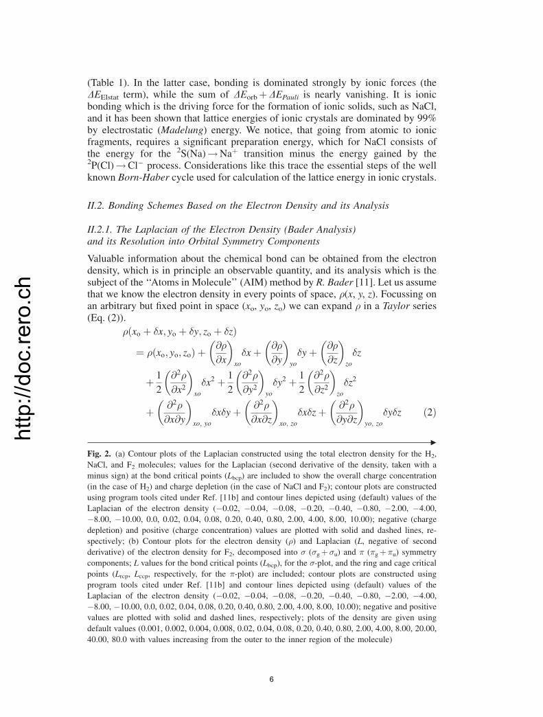
Fig. 2. (a) Contour plots of the Laplacian constructed using the total electron density for the H2,

NaCl, and F2 molecules; values for the Laplacian (second derivative of the density, taken with a

minus sign) at the bond critical points (Lbcp) are included to show the overall charge concentration

(in the case of H2) and charge depletion (in the case of NaCl and F2); contour plots are constructed

using program tools cited under Ref. [11b] and contour lines depicted using (default) values of the

Laplacian of the electron density (�0.02, �0.04, �0.08, �0.20, �0.40, �0.80, �2.00, �4.00,

�8.00, �10.00, 0.0, 0.02, 0.04, 0.08, 0.20, 0.40, 0.80, 2.00, 4.00, 8.00, 10.00); negative (charge

depletion) and positive (charge concentration) values are plotted with solid and dashed lines, re-

spectively; (b) Contour plots for the electron density (�) and Laplacian (L, negative of second

derivative) of the electron density for F2, decomposed into � (�gþ �u) and � (�gþ�u) symmetry

components; L values for the bond critical points (Lbcp), for the �-plot, and the ring and cage critical

points (Lrcp, Lccp, respectively, for the �-plot) are included; contour plots are constructed using

program tools cited under Ref. [11b] and contour lines depicted using (default) values of the

Laplacian of the electron density (�0.02, �0.04, �0.08, �0.20, �0.40, �0.80, �2.00, �4.00,

�8.00, �10.00, 0.0, 0.02, 0.04, 0.08, 0.20, 0.40, 0.80, 2.00, 4.00, 8.00, 10.00); negative and positive

values are plotted with solid and dashed lines, respectively; plots of the density are given using

default values (0.001, 0.002, 0.004, 0.008, 0.02, 0.04, 0.08, 0.20, 0.40, 0.80, 2.00, 4.00, 8.00, 20.00,

40.00, 80.0 with values increasing from the outer to the inner region of the molecule)

6

http://doc.rero.ch

The first and second derivatives in Eq. (2) define a vector r��!and a (symmetric)

matrix of second derivative (Hessian) H (Eq. (3)).

ðrq�!Þr0 ¼

@�@x

� �xo

@�@y

� �yo

@�@z

� �zo

0BBBB@

1CCCCA; ðHÞr0 ¼

@2�@x2

� �xo

@2�@x@y

� �xo; yo

@2�@x@z

� �xo; zo

@2�@y@x

� �yo; xo

@2�@y2

� �yo

@2�@y@z

� �yo; zo

@2�@z@x

� �zo; xo

@2�@z@y

� �zo; yo

@2�@z2

� �zo

266664

377775 ð3Þ

7

http://doc.rero.ch

Their components can easily be calculated from the knowledge of the density �ð~rrÞon a 3D grid, as available from most quantum chemistry codes.

The topological analysis of ðrq�!Þr0 makes it possible to locate stationary points

in � which might correspond to local minima, maxima, or saddle points. Theyfurther allow to identify atoms or fragments of atoms in a molecule or atomicsubspaces bordered by surfaces S (basins) on which the flux of the gradientvanishes (Eq. (4)) where ðrq

�!ÞS is calculated at each point of the surface, nS! is

any vector perpendicular to the surface.

ðrq�!ÞS � nS!¼ 0 ð4Þ

It has been shown that the virial theorem holds for these basins and integrationof � over them allows to get atomic or fragment charges within the molecule. Thematrix (H)ro allows to calculate the Laplacian of the electron density as a sum of itsdiagonal elements (Eq. (5)), which is invariant with respect to the choice of thecoordinate system.

L ¼ � 1

2

@2�

@x2

� �xo

þ 1

2

@2�

@y2

� �yo

þ 1

2

@2�

@z2

� �zo

ð5Þ

Diagonalization of the matrix H, leading to principle curvatures as the eigenvaluesand principal axis as the eigenvectors allows to explore the topology of the electrondensity at any given point of space. The values of these quantities at the pointswhere ðrq

�!Þ vanishes (critical points) are of particular interest. They are usuallydenoted by (r, s), with r standing for the rank (number of non-zero eigenvalues) ands for the signature (sum of signs of the eigenvalues). Bond critical points, denotedas (3, �1) are such, where two eigenvalues are negative, while one is positivecorresponding to (two) maxima and one minimum with respect to the directionsdefined by the eigenvectors. The eigenvector for the positive eigenvalue connectstwo atoms and defines a bond path between them. Positions of the nuclei arecharacterized by a maximum of � [(3, �3) critical points, or nuclear attractors].Furthermore one finds ring and cage critical points where two or three eigenvalues(curvatures) of H are positive, (3, 1) and (3, 3); examples are given by cyclic(cyclopropane) and cage shaped (P4) molecules, respectively. It has been shownthat the values of L at each point (Eq. (5)) can be related with the kinetic G(r) andwith the potential V(r) energy density at that point (Eq. (6)) where positive andnegative values of (L) characterize regions in space in which charge is accumulatedor depleted, respectively.

2Gð r!Þ þ Vð r!Þ ¼ �Lð r!Þ ð6ÞIn Fig. 2 we show three typical examples, two for one electron pair bonding (H2

and F2) and one for a typical ionic molecule as NaCl. As expected, electroniccharge concentration and depletion between the nuclei of H2 and NaCl is observed.However, for F2 we don’t see any increase of L between the nuclei. As has beenpointed out by Cremer and Kraka for F2 [18], L is negative at the bond critical pointrc (�2.908 e.A�5), but still, the sum of G(rc)þV(rc)(¼2.247–4.292¼ �2.045Hartree. A�3) results in a negative value of the total energy density (E¼GþV).The unusual bonding in F2 has been explained by VB-theory [19] in terms of a verystrong mixing between covalent and ionic resonance structures due to a large and

8

http://doc.rero.ch

negative resonance integral � in which the kinetic energy term dominates [20].This has been called a ‘‘charge shift bonding’’ [19]. It is interesting and importantto note that (�L) can still reflect these results when decomposed into contributionsfrom � and � character – [�L(�)] and [�L(�)], respectively. Figure 2b nicelyshows this; thus the plot of [�L(�)] displays two electron pairs between the Fnuclei, each belonging to its closest nuclei but with a clear deformation orientedtoward the neighbouring nucleus. Also the �-lone pairs are clearly discerned, aswell as the �-oriented lone pairs on F, which now, due to the Pauli-repulsion areoriented in a direction outwards the F–F bond axis.

The distinction between orbitaly resolved contributions in L and in ELF (seenext section) plays a central role in our analysis of the TM–ligand bond as we shallsee in Section III.

Finally, it is worth mentioning that the electron pair density in conjunction withthe AIM theory enables one to determine the average number of electron pairs thatare localized to each atom (A) and the number that are formed between any givenpair of atoms A and B. Within this quantitative AIM framework [21] atomic loca-lization and delocalization indices noted �(A) and �(A, B) have been defined, thelatter being sometimes referred to as bond orders. Applications of this approach tocharacterize metal–ligand bonding in TM di- and tri-halides have already beenreported [22].

II.2.2. The Electron Localization Function (ELF)

The introduction of the electron localization function (ELF) by Becke andEdgecombe in 1990 [12] has lead to a quantitative index to describe intuitiveconcepts like chemical bond and electron pair. This function allows to describein a topological way a quantity related to the Pauli exclusion principle. The localmaxima of this function define ‘localization domains’ of which there are onlythree basic types: valence domains (bonding, non-bonding) and core domains(see below). The spatial organization of localization domains provides a basisfor a well-defined classification of bonds. An obvious advantage of this functionis that it can be derived from computed and experimental electron densities.

The electron localization function has been originally derived from the condi-tional probability of finding an electron of spin � at r0 when an electron with thesame spin is located at~rr. As proposed by Becke and Edgecombe, ELF is a simplefunction taking values between 0 to 1 and measuring the excess local kineticenergy due to the Pauli repulsion.

For a single determinental wavefunction built from Hartree-Fock or Kohn-Sham orbitals ’i and an electron density �� the value of ELF is given by Eq. (7)where D� and D0

� are described by Eqs. (8) and (9).

ELF ¼ 1

1þ ðD�

D0�Þ2 ð7Þ

D� ¼XNi¼1

jr’ij2 � 1

4

jr��j2��

ð8Þ

9

http://doc.rero.ch

D0� ¼

3

5ð6�2Þ2=3�5=3� ð9Þ

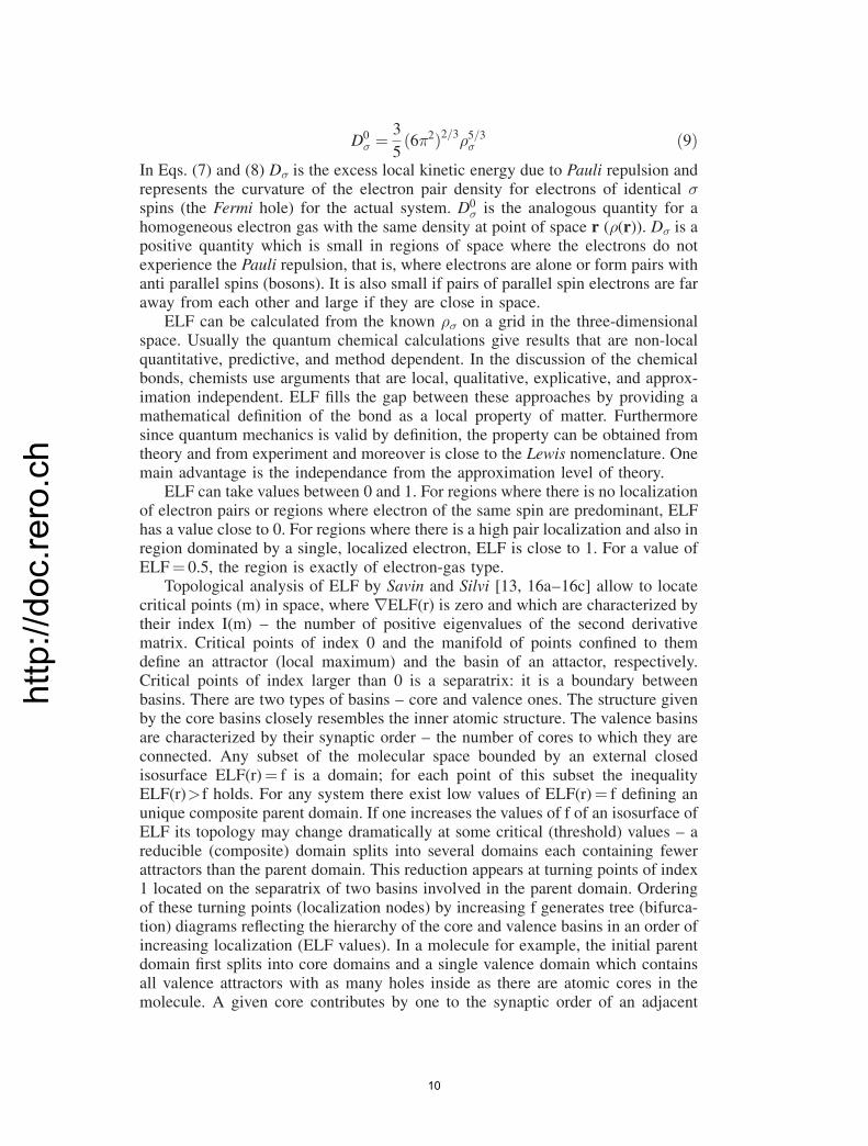
In Eqs. (7) and (8) D� is the excess local kinetic energy due to Pauli repulsion andrepresents the curvature of the electron pair density for electrons of identical �spins (the Fermi hole) for the actual system. D0

� is the analogous quantity for ahomogeneous electron gas with the same density at point of space r (�(r)). D� is apositive quantity which is small in regions of space where the electrons do notexperience the Pauli repulsion, that is, where electrons are alone or form pairs withanti parallel spins (bosons). It is also small if pairs of parallel spin electrons are faraway from each other and large if they are close in space.

ELF can be calculated from the known �� on a grid in the three-dimensionalspace. Usually the quantum chemical calculations give results that are non-localquantitative, predictive, and method dependent. In the discussion of the chemicalbonds, chemists use arguments that are local, qualitative, explicative, and approx-imation independent. ELF fills the gap between these approaches by providing amathematical definition of the bond as a local property of matter. Furthermoresince quantum mechanics is valid by definition, the property can be obtained fromtheory and from experiment and moreover is close to the Lewis nomenclature. Onemain advantage is the independance from the approximation level of theory.

ELF can take values between 0 and 1. For regions where there is no localizationof electron pairs or regions where electron of the same spin are predominant, ELFhas a value close to 0. For regions where there is a high pair localization and also inregion dominated by a single, localized electron, ELF is close to 1. For a value ofELF¼ 0.5, the region is exactly of electron-gas type.

Topological analysis of ELF by Savin and Silvi [13, 16a–16c] allow to locatecritical points (m) in space, where rELF(r) is zero and which are characterized bytheir index I(m) – the number of positive eigenvalues of the second derivativematrix. Critical points of index 0 and the manifold of points confined to themdefine an attractor (local maximum) and the basin of an attactor, respectively.Critical points of index larger than 0 is a separatrix: it is a boundary betweenbasins. There are two types of basins – core and valence ones. The structure givenby the core basins closely resembles the inner atomic structure. The valence basinsare characterized by their synaptic order – the number of cores to which they areconnected. Any subset of the molecular space bounded by an external closedisosurface ELF(r)¼ f is a domain; for each point of this subset the inequalityELF(r)>f holds. For any system there exist low values of ELF(r)¼ f defining anunique composite parent domain. If one increases the values of f of an isosurface ofELF its topology may change dramatically at some critical (threshold) values – areducible (composite) domain splits into several domains each containing fewerattractors than the parent domain. This reduction appears at turning points of index1 located on the separatrix of two basins involved in the parent domain. Orderingof these turning points (localization nodes) by increasing f generates tree (bifurca-tion) diagrams reflecting the hierarchy of the core and valence basins in an order ofincreasing localization (ELF values). In a molecule for example, the initial parentdomain first splits into core domains and a single valence domain which containsall valence attractors with as many holes inside as there are atomic cores in themolecule. A given core contributes by one to the synaptic order of an adjacent

10

http://doc.rero.ch

valence basin. The partition of reducible domains into core and valence domains iscalled core=valence bifurcation. It can occur in two different ways: either the coreirreducible domains split before the valence ones, or the core=valence separationtakes place after the valence division into two or more domains. While the firstprocess is characteristic for molecules or molecular ions, the second one is char-acteristic for weak interactions among fragments. An ELF study on VOþ

x and VOx

(x¼ 1–4) clusters based on the analysis of the bifurcation of the localizationdomains [23] provides a valuable information about the V–O bond and will bediscussed in the context of our results in Section III.3.

We can conclude, that the topological analysis of the gradient field of ELFprovides a framework for the partition of the molecular space into basins of attrac-tors having a clear chemical meaning. While basin populations are evaluated byintegrating the one-electron density over basins, the variance of the basin popula-tions provides a measure of the delocalization. An application of this approachto study geometries of formally d0 MXn (X¼ F,H,CH3, and O; M¼Ca to Mn,n¼ 2–6) contributes to understanding of their non-VSEPR geometries [24]. Anoverview of the possibilities offered by the topological analysis of ELF rangingfrom isolated atoms to solids may be found elsewhere [13, 22, 25].

We should finally note, that applications of AIM and ELF gain interpretativepower when separated into components of different symmetry. It has been shown,for example, that the separation of ELF into its � and �-components in aromaticmolecules allows to quantify the concept of resonance and to set up a scale foraromaticity [26]. A possible justification of this approach could be done by re-expressing ELF in terms of time independent electron transition current densitiesbetween occupied orbitals [27].

II.3. Angular Overlap Model [28–31]

The energies of the d-orbitals for complexes with ligand to metal donor acceptorbonds are described by energies for �¼ � and �-antibonding, which pertain to wellaligned metal 3d- and ligand p-orbitals, e�. Using perturbation theory and theWolfsberg-Helmholz approximation for the resonance integral H(M-L)� one obtainsEq. (10) for e�, showing a quadratic dependence on the group overlap integral S�.

e�ffi H M � Lð Þ2�HM� HL

� H2L

HM� HL

� S2� ð10Þ

e� parameters can be obtained using spectral information from a fit of ligandfield expressions. For an octahedral complex only one ligand field splitting param-eter (Eq. (11)) can be derived which do not allow to separate e� and e�.

10Dq ¼ 3e�� 4e� ð11ÞThis situation changes when going to symmetric complexes. Figure 3 illustrates

this for a square-pyramidal ML5 complex where also AOM expressions for theenergies of the d-orbitals are given. For a non centro-symmetric complex a mixingof jsi and jpi into the jdi orbitals of the TM is possible. This is particularly pro-nounced for the dz2-4s mixing that leads to lowering of the dz2 orbital in energy,

11

http://doc.rero.ch

which is described by an additional parameter DE3d-4sp and which is known tobecome mostly non-bonding in the limiting case of a square-planar complex[32–33]. DFT calculations enable to use Kohn-Sham orbital energies to get valuesof 3e�,e� and DE3d-4sp, and to compare these with the results obtained from ETSbonding analysis, pertaining to all occupied orbitals. Thus a clear distinctionbetween bonding and antibonding contributions becomes possible and will be dis-cussed together with the analysis based on the electron density (Laplacian and ELF).

II.4. Computational Details

DFT calculations and bonding analysis in this work have been performed using theAmsterdam Density Functional (ADF) program [10] (release 2004.01) using thePerdew-Wang (PW91) gradient corrected functional. Triple zeta basis sets (TZP) asprovided by the program data base have been taken for the calculations. Geometryoptimizations allowing to fix the geometry of every complex have been carried outusing the LDA implemented in the VWN-functional. This procedures are known toyield TM–ligand bond distances in good agreement with experiments.

The octahedral MIIIX63� complexes studied in this work are highly negative

charged. One may ask how bonding is affected by a charge compensating medium

Fig. 3. Splitting of the d-orbitals in a quadratic pyramidal TM complex with five ligands – four

equatorial, one axial; parameterization of these energies in terms of the angular overlap model

without (left) and with 3d-4s, 4p mixing (right) is given along with the unperturbed 3d (left) and

4s, 4p (right) orbitals; e�(ax), e�(ax) and e�(eq), e�(eq) pertain to antibonding energies due to the

axial and equatorial ligands, respectively, and DE3d-4sp energies reflect the stabilization of the 3dz2orbital by mixing with mostly (4s) and to lesser extent with the (4p) orbital; the lowering of energy of

the e(dxz,dyz) orbital due to mixing with the 4px, 4py functions is neglected; these equations have

been used to deduce AOM parameters e� and e� from KS-DFT calculations on the ground state of

CrIIIX5 (X¼H2O,F,Cl,Br,I) (Table 5) with all Cr-X bond lengths taken to be the same as those for the

corresponding octahedral CrIIIX6 species

12

http://doc.rero.ch

(solvent in solutions or counter ions in the solid). To mimic this effect and study itsinfluence on the bonding and ligand field parameters we have chosen CrCl6

3� as anexample and used the conductor-like screening model (COSMO [34]) as imple-mented in ADF [35]. Solvent radii of 1.75 and 0.97 A have been selected for Cl andCr. The dielectric constant and the solvent radius " has been fixed at 78.4 and 1.4 A,respectively (pertaining to water as a solvent) [36].

Topological analyses of the electron density have been made using two homemade programs written in Matlab: one for Bader analysis (Emma1) and anotherone (Emma2) for ELF calculations [37]. Both programs are interfaced with theADF program package and make use of the tape21 file and the ‘‘densf’’ utilityprogram, the latter providing the electron density on a grid.

To calculate the orbitally resolved Laplacian and ELF values we utilized thehigh symmetry of the systems and used non-zero electronic ground state occupa-tions, taking SCF Kohn-Sham orbitals of a given symmetry, while ignoring allorbitals of a different symmetry (by setting zero occupation numbers in the input).

III. Results and Discussions

III.1. Complexes with CN¼6

III.1.1. Halide Complexes of CrIII, CoIII, MoIII, WIII

MO energy diagrams for the bare CrIIIX63� (d3, 4A2g ground state, X¼ F�,Cl�Br� –

Fig. 4) anions show the pattern for an octahedral complex, with bonding a1g,eg,t2g,and t1u MOs that are dominated by ligand and antibonding MOs dominated by

Fig. 4. KS-MO energy (in eV) diagram for CrX63�(X¼ F,Cl,Br) charge uncompensated species;

contributions (in percentages) from the Cr 3d, 4s (in ‘‘( )’’ brackets) and 4p (in square ‘‘[ ]’’ brackets)

are given

13

http://doc.rero.ch

metal orbitals, i.e., typical for ligand to metal donor–acceptor bonds. It can bequalitatively understood by the following expressions for the stabilization=destabilization of the ligand=metal orbitals obtained from the angular overlapmodel (Eq. (12a)) and the qualitative order for the magnitude of the AOM param-eters as given by Eq. (12b).

�Eða1gÞ ¼ � 6e�ð4sÞ½ ��Eðt1uÞ ¼ � 2e�ð4pÞ þ 4e�ð4pÞ½ ��EðegÞ ¼ � 3e�ð3dÞ½ ��Eðt2gÞ ¼ � 4e�ð3dÞ½ � ð12aÞ

e�ð4pÞ; e�ð4pÞ<e�ð4sÞ<e�ð3dÞ<e�ð3dÞ ð12bÞMixing between metal and ligand orbitals is largest for the metal 3d- and muchsmaller, but not negligible for the metal 4s- and 4p-orbitals. The participation ofthe j4si and j4pi orbitals to bonding increases when going from F to Cl to Brcomplexes, which is generally fulfilled also for the other coordination numbers withthe same ligands (see below). For CrF6

3� we notice the anomalous position of the3a1g(4s) MO, being found below the 2t2g and 3eg MOs. This is clearly an artifactconnected with the choice of the orbital exponent and possibly the additional effectof the uncompensated high negative charge of the anion. Going to Cl and Br,the correct ordering 2t2g<3eg<3a1g is restored, but still, the position of 3a1g(4s)is far too low. Thus, for free Cr3þ we calculate j4si as lying 11 eV above the j3diorbitals. To compensate for the negative cluster charge, COSMO calculations forCrX6

3�(X¼ F,Cl) have been performed. Their MO diagrams are compared withthose of the bare anions in Fig. 5. The contribution of a charge compensating solvent

Fig. 5. The effect of charge compensating solvent continuum on the KS-MO energies (right) in

comparison with those calculated using bare anions (left) for CrF63� and CrCl6

3� as studied using a

COSMO model with solvent parameters taken for water (see text)

14

http://doc.rero.ch

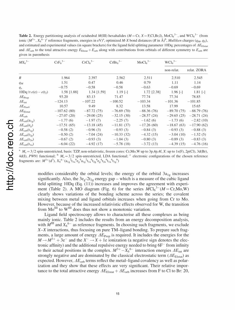
modifies considerably the orbital levels; the energy of the orbital 3a1g increasessignificantly. Also, the 3eg-2t2g energy gap – which is a measure of the cubic ligandfield splitting 10Dq (Eq. (11)) increases and improves the agreement with experi-ment (Table 2). A MO diagram (Fig. 6) for the series MCl6

3�(M¼Cr,Mo,W)clearly shows variations of the bonding scheme across the series; the covalentmixing between metal and ligand orbitals increases when going from Cr to Mo.However, because of the increased relativistic effects observed for W, the transitionfrom MoIII to WIII does thus not show a monotonic variation.

Ligand field spectroscopy allows to characterise all these complexes as beingmainly ionic. Table 2 includes the results from an energy decomposition analysis,withMIII and X6

6� as reference fragments. In choosing such fragments, we excludeX–X interactions, thus focusing on pure TM–ligand bonding. To prepare such frag-ments, a large amount of energy DEPrep is required. It includes the energies for theM!M3þ þ 3e� and the X� !Xþ 1e ionization (a negative sign denotes the elec-tronic affinity) and the additional repulsive energy needed to bring 6F� from infinityto their actual positions in the complex. M3þ�X6

6� interaction energies DEint arestrongly negative and are dominated by the classical electrostatic term (DEElstat) asexpected. However, DEorb terms reflect the metal–ligand covalency as well as polar-ization and they show that these effects are very significant. Their relative impor-tance to the total attractive energy DEElstatþDEorb increases from F to Cl to Br: 20,

Table 2. Energy partitioning analysis of octahedral M(III) hexahalides (M¼Cr, X¼F,Cl,Br,I), MoCl63�, and WCl6

3� (from

ionic ðM3þ, X66�)c reference fragments, energies in eV)a, optimizedM-X bond distances (R in A)b,Mulliken charges (qM, qX),

and estimated and experimental values (in square brackets) for the ligand field splitting parameter 10Dq; percentages of DEElstat

and DEorb to the total attractive energy EElstatþEorb along with contributions from orbitals of different symmetry to Eorb are

given in parenthesis

MX63� CrF6

3� CrCl63� CrBr6

3� MoCl63� WCl6

3�

non-relat. relat. ZORA

R 1.964 2.397 2.562 2.511 2.510 2.545

qM 1.51 0.47 0.46 0.79 1.11 1.14

qx �0.75 �0.58 �0.58 �0.63 �0.69 �0.69

10Dqffi e(e)� e(t2) 1.58 [1.88] 1.34 [1.59] 1.19 [-] 1.72 [2.38] 1.96 [-] 1.81 [-]

DEPrep 93.20 83.13 71.47 77.74 77.34 78.85

DEint �124.13 �107.22 �100.52 �103.34 �101.36 �101.85

DEPauli 10.57 9.49 8.32 13.58 17.99 15.65

DEElstat �107.62 (80) �87.72 (75) �76.69 (70) �88.36 (76) �89.70 (75) �88.79 (76)

DEorb �27.07 (20) �29.00 (25) �32.15 (30) �28.57 (24) �29.65 (25) �28.71 (24)

DEorb(a1g) �1.77 (6) �1.97 (7) �2.25 (7) �1.62 (6) �1.73 (6) �2.82 (10)

DEorb(eg) �17.51 (65) �13.18 (45) �11.81 (37) �17.26 (60) �18.67 (63) �17.90 (62)

DEorb(t1g) �0.58 (2) �0.96 (3) �0.93 (3) �0.84 (3) �0.93 (3) �0.88 (3)

DEorb(t2g) �0.50 (2) �7.04 (24) �10.33 (32) �4.32 (15) �3.04 (10) �1.52 (5)

DEorb(t2u) �0.67 (2) �0.93 (3) �1.04 (3) �0.80 (3) �0.89 (3) �0.83 (3)

DEorb(t1u) �6.04 (22) �4.92 (17) �5.78 (18) �3.72 (13) �4.39 (15) �4.76 (16)

a Ms¼ 3=2 spin-unrestricted, basis: TZP, non-relativistic, frozen cores: Cr,Mo,W up to 3p,4p,4f, X: up to 1s(F), 2p(Cl), 3d(Br),

4d(I), PW91 functional; b Ms¼ 3=2 spin-unrestricted, LDA functional; c electronic configurations of the chosen reference

fragments are: M3þ(d3), X66�(a1g

2t1u6eg

4a1g2t1u

6t2g6eg

4t2u6t1u

6t1g6)

15

http://doc.rero.ch

25, and 30% for the covalency and �27.07, �29.00 and �32.15 eV for the magni-tude, respectively. This is consistent with the chemical intuition: i.e., increase ofthe Cr–X covalency when going from F to Cl to Br. A closer look at the orbitaldecomposition of DEorb, shows however, that contributions from j4si and j3di orbit-als to � bonding (reflected by the a1g and eg energy terms), �þ � bonding (t1u), and�-bonding (t2g) behave in a different way across the {F,Cl,Br} series. The eg and t1uenergies decrease, while the energies of t2g, and a1g increase in this order. Thus, thetrend observed in DEorb is the result of a subtle balance between contributions fromdifferent bonding interactions. The behaviour of the eg and t2g orbitals also explainsthe lowering of 10Dq when going from F to Br as a result of the decreasing eg-�antibonding interaction. The account for solvation shows a strong stabilization of theanion due to solute–solvent interactions which are larger for F�, than for Cl�.However, only the metal (3d)-ligand �-bonding is stabilized by the solvent. Table3, where the various contributions of the components obtained in the energy decom-position are listed, clearly shows this. Contributions from orbitals other than from egare positive and do sum up to yield a small, yet, positive value of �DEorb.

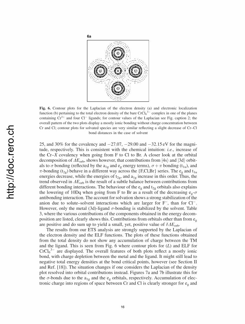
The results from our ETS analysis are strongly supported by the Laplacian ofthe electron density and the ELF functions. The plots of these functions obtainedfrom the total density do not show any accumulation of charge between the TMand the ligand. This is seen from Fig. 6 where contour plots for (L) and ELF forCrCl6

3� are displayed. The overall features of both plots reflect a mostly ionicbond, with charge depletion between the metal and the ligand. It might still lead tonegative total energy densities at the bond critical points, however (see Section IIand Ref. [18]). The situation changes if one considers the Laplacian of the densityplot resolved into orbital contributions instead. Figures 7a and 7b illustrate this forthe �-bonds due to the a1g and the eg orbitals, respectively. Accumulation of elec-tronic charge into regions of space between Cr and Cl is clearly stronger for eg and

Fig. 6. Contour plots for the Laplacian of the electron density (a) and electronic localization

function (b) pertaining to the total electron density of the bare CrCl63� complex in one of the planes

containing Cr3þ and four Cl� ligands; for contour values of the Laplacian see Fig. caption 2; the

overall pattern of the two plots display a mostly ionic bonding without charge concentration between

Cr and Cl; contour plots for solvated species are very similar reflecting a slight decrease of Cr–Cl

bond distances in the case of solvent

16

http://doc.rero.ch weaker for a1g. Also the presence on lone pairs densities on the ligands in regions

of space opposite to the metal–ligand bond direction is obvious. These featuresbecome even more pronounced when looking at the ELF plots. In Figs. 8a and 8bwe compare contours for ELF resolved into �(eg) and �(t2g), respectively. It fol-lows, that localization valence domains are much more pronounced for the �-density, when compared to the �-density. They are shifted from the midpoint ofthe Cr–Cl bond vector toward the ligand in agreement with electronegativity

Table 3. Changes of DEorb and of its components of different symmetry going from bare CrF63� and

CrCl66� to solvated species (�DEorb); solute–solvent interaction energies for hydrated species (Esolv)

and changes of the values of 10Dq (�(10Dq), all energies in eV) and of the Cr–F and Cr–Cl optimized

bond lengths (�R, in A) are also included

Changes ðCrX63�Þbare ! ðCrX6

3�Þsolv X¼ F Cl

�DEorb 0.259 0.294

�DEorb(a1g) 0.100 0.158

�DEorb(eg) �0.779 �0.797

�DEorb(t1g) 0.285 0.197

�DEorb(t2g) 0.072 �0.026

�DEorb(t2u) 0.281 0.224

�DEorb(t1u) 0.328 0.539

Esolv �21.520 �17.598

�(10Dq) 0.355 0.112

�R �0.06 �0.06

Fig. 7. Contour plots for the Laplacian of the electron density using � densities resolved into a1g(a) and eg (b) symmetry components; plots are given for one of the planes containing Cr3þ and four

Cl� ligands and values of the Laplacian for the contour lines are the same as specified in Fig. caption

2; solid lines depict charge concentrations into bonding (between Cr and Cl) and lone-pair domains,

which are more pronounced for the eg electron density and less pronounced, yet clearly discernible

for the a1g electron density

17

http://doc.rero.ch

18

http://doc.rero.ch

considerations. It should be pointed out, however, that Cr–Cl �-bonding is weak-ened by admixture of the antibonding (2t2g)

3 configuration. Figure 8c exhibitsthis behavior in an impressive way: when constructing this plot, the three d-elec-trons on the antibonding 2t2g MO have been removed and the picture reflects theeffect of the �-bonding electrons only. Finally, Fig. 8d illustrates that valence j4piorbitals can not be neglected in the discussion of the TM–ligand bond. This is inagreement with the energy decomposition analysis, which tends to show that forCrCl6

3�, j4pi orbitals seem to participate to bonding even stronger than j4si ones.

III.1.2. Aquo-Complexes of CrIII and CoIII

Water is considered to form highly anisotropic �-bonds with transition metals suchas TiIII(d1), VIII(d2), and MnIII(high-spin d4) as this is convincingly shown by EPRand electronic Raman studies of the corresponding complexes [38–40]. However,analysis of bonding in these complexes is complicated by the presence of Jahn-Teller effect. The ground states are orbitally degenerate – 2T2(d

1), 3T1(d2), and

4E(d4), respectively, and these studies mostly focused on this effect. To charac-terize TM–H2O bonds, we have chosen CrðH2OÞ63þ with jð2t2gÞ3; 4A2gi, andCoðH2OÞ63þ with jð2t2gÞ6;1 A1gi ground state as test cases. Energy decompositionanalyses have been carried out for a single H2O molecule interacting with aMðH2OÞ53þ (M¼Cr3þ,Co3þ) fragment (Table 4). In agreement with the loweringof M–O bond length when going from left to right in the TM series, the total bondenergy of one H2O is larger for Co than for Cr. The bonding interaction is domi-nated mostly by the electrostatic term DEElstat, but orbital interaction is found toplay an important role as well. Covalent bonding terms are calculated to be muchstronger for � than for � interactions, as expected. In agreement with the smallernumber of electrons occupying the antibonding 3d� orbitals (3 for Cr and 6 for Co)and in spite of the lower bond distance for Co, �-bonding energy for Cr–OH2 isfound to be about two times larger than for Co–OH2. It is very surprising that

1Fig. 8. The electronic localization function for CrCl6

3� in one of the planes containing Cr3þ and

four Cl� ligands constructed partitioning the electron density into eg, Cr(3d)–Cl � (a), t2g, Cr(3d)–Cl

� (b, c), and t1u, Cr(4p)–Cl �þ� (d) components; the contour plots for the t2g density (b, c) reflects

the weakening effect on the Cr–Cl bond caused by the three antibonding t2g(3d) electrons, which

have been accounted for in the plot (b) but ignored in the plot (c)

Fig. 9. Electronic localization function for CoðH2OÞ63þ with a Th geometry (treated in its D2h

subgroup by ADF); contour plots are based on the total electron density in (a) and on its ag symmetry

component in (b); the irreducible representations (irreps) spanned by the valence orbitals of the

transition metals give rise to the following irreps of the D2h subgroup: eg(dz2, dx2–y2)! ag(dz2,

dx2–y2), tg(dxy, dxz, dyz)! b1g(dxy), b2g(dxz), b3g(dyz); ag(4s)! ag, tu(4px, 4py, 4pz)! b1u(4px),

b2u(4py), b3u(4px); thus the plot in (b) reflects the combination of bonding effects with participation

of the dz2, dx2–y2, and 4s valence orbitals of the TM

Fig. 11. Contour plots for the electron localization function of CrF4 with a Td geometry within a

plain containing a CrF2 molecular fragments constructed using the total electron density (a) and its

partitioning into a1 (b), t2 (c), and e (d) symmetries; the plots reflect the participation of the Cr 4s �

(a1), 3d and 4p �þ� (t2), and 3d � (e) to the Cr–F bonding in (b), (c), and (d), respectively

19

http://doc.rero.ch

�-anisotropy is not very pronounced, when comparing �-bonding energies within(b2) and out of (b1) the TM–OH2 plane. Only for Cr(III) we do observe jDEorbðb1Þj>jDEorbðb2Þj. Apparently, when considering bonding energies, �-anisotropy does notshow up in our analysis.

Using the energies of the Kohn-Sham orbitals with dominant metal character ofthe fivefold coordinated fragments (see Fig. 3) we could estimate the correspondingAOM-parameters which are listed in Table 4. The values obtained for e�s and e�care in agreement with the usual assumption made in LF theory, namely, that out-of-plane �-antibonding is larger than in the TM–OH2 plane. Finally, the variation ofthe respective e� and e� parameters do compensate in 10Dq leading to values ofthis latter parameter which are quite close in magnitude for Cr and Co. Using thesame approach, i.e., considering CrX5

2�(X¼ F,Cl,Br) fragments it was possible tocalculate AOM parameters for Cr–X bonds. All these results are gathered in Table5 and compared with values obtained from spectral data. There is a good overallagreement between the two sets of data and this shows that DFT calculations dowell reproduce the trends observed experimentally.

Finally, the metal–ligand covalency is nicely expressed in the ELF function forCoðH2OÞ63þ (Fig. 9), both are derived from the total density (Fig. 9a) and from its

Table 4. Energy partitioning analysis for octahedral Cr(III) and Co(III) hexa-aquo complexes cal-

culated starting from MðH2OÞ52þ (M¼CrIII, d3ðt2g3Þ and CoIII, d6ðt2g6Þ) complex units with the

octahedral bond distances and bond angles and adding a sixth H2O ligand to complete the coordination

sphere to the octahedron; deduced values of the AOM parameters e�, e�s(?H2O plane), and e�c(jjH2O

plane) are also given; energy values are listed in eVa, optimized Cr(Co)–OH2 bond distances (R) in Ab

MðH2OÞ63þ M¼ CrIII CoIII

R 1.971 1.888

DEPauli 2.583 3.140

DEElstat �2.985 �3.481

DEorb �2.224 �2.521

DEint �2.627 �2.862

DEorb(a1) � �1.397 �2.005

DEorb(b1, xz, �?H2O-plane) �0.512 �0.245

DEorb(b2, yz, �jjH2O-plane) �0.306 �0.265

e� 1.277 1.331

e�s(? H2O plane) 0.448 0.614

e�c(jj H2O plane) 0.070 0.018

10Dq¼ 3e�� 2e�s� e�c 2.795 2.729

a Spin-restricted calculation, basis: TZP, non-relativistic, frozen cores: Cr(Co) up to 3p, O: up to 1s,

PW91 functional; b spin-restricted, LDA functional

Table 5. AOMparameters (in eV) from LFDFTanalysis and from experiment (in parenthesis, adopted

from Refs. [8, 9]) using optical data for hexacoordinate Cr(III) complexes

Ligand H2O F Cl Br I

e� 1.23 (0.93) 1.08 (0.92) 0.70 (0.68) 0.61 (0.61) 0.52 (0.53)

e� 0.26 (0.17) 0.37 (0.21) 0.18 (0.11) 0.15 (0.07) 0.11 (0.07)

20

http://doc.rero.ch

a1(�) components. The results clearly show the domination of the � over the �interactions, in full support of our energy decomposition analysis (Table 4).

III.2. Neutral Complexes with CN¼4 – Tetrahedral Tetrahalides of CrIV

The KS–MO diagram for the CrX4 (X¼ F,Cl,Br,I) series with a jð2eÞ2 2A2i groundstate (Fig. 10) shows the pattern for an tetrahedral complex, with the bonding – 2t2,2a1, 1e and the anitibonding 2e, 4t2, 3a1 (not shown) MOs dominated by ligand(p, s) and metal (3d, 4s) orbitals, respectively. Thus, as in the complexes withCN¼6 we have a typical pattern for a ligand-to-metal donor–acceptor bond. InFig. 10 we also display the fully occupied (by ligand electrons) strictly (t1) andapproximately (3t2) non-bonding MOs. The order of the MOs can qualitatively beunderstood by the energy decrease=increase of ligand=metal centered orbitalsgiven by the AOM (Eq. (13)) and the inequalities following Eq. (12b).

�Eða1Þ ¼ � 4e�ð4sÞ½ �

�EðeÞ ¼ � 8

3e�ð3dÞ

� �

�Eðt2Þ ¼ � 4

3e�ð3dÞ þ 8

9e�ð3dÞ

� �

�Eðt2Þ ¼ � 4

3e�ð4pÞ þ 8

3e�ð4pÞ

� �ð13Þ

Fig. 10. KS-MO diagram for tetrahedral CrX4 (X¼ F,Cl,Br,I) molecules in their jð2eÞ2; 3A2i groundstate; percentages of contributions from the 3d, 4s, and 4p orbitals are indicated (without, with ‘‘( )’’,

and ‘‘[ ]’’ brackets, respectively)

21

http://doc.rero.ch

MO population analyses reflect a very pronounced covalency, which increaseswhen going from the fluoride to the iodide complex. In the same order the partic-ipation of j4si to bonding increases; this is reflected by the contribution of the j4siatomic orbital to the 2a1 MO and its energy lowering when going from CrF4 toCrCl4. The plot of the ELF using the total electron density for CrF4 shows a mostlyionic pattern. A similar plot is obtained for the Laplacian of the electron density(Fig. 11a). However, a partitioning of the density into different symmetries shows,for a1 and t2, localization of bonding pairs between Cr and F (Figs. 11b, 11c). Inspite of the fact that �- and �-bonding are not separable for Td it seems thatlocalization of valence domains is mainly due to �-overlap: the localization of�-bonding pairs (e-symmetry) is not very pronounced (Fig. 11d). In order, not tobe biased by the choice of fragments, ETS energy decomposition analyses havebeen performed using both neutral (CrþX4) and ionic (Cr4þ þ X4

4�) fragmentswhose results are listed in Table 6. Looking at the jDEorbj term, we notice that itdecreases from the F to I when taking neutral fragments and it increases in thatdirection for ionic fragments. It is only the latter case which is consistent withthe MO diagram (increase of covalency from F to I) as depicted in Fig. 10. Alsothe electrostatic energy jDEElstatj behaves as expected: being largest for CrF4and smallest for CrI4. The trend in the total attractive energy DEorb þ DEElstat isfinally the one which also determines the behavior of the total bonding energy –decrease of jDEintj across the X¼ F to I series. It is the DEElstat term whichdominates this trend. Let us now concentrate on DEorb in case of ionic referencefragments. Here the behavior is different to the octahedral complexes: i.e., all ofits components, jDEorbða1Þj, jDEorbðeÞj, and jDEorbðt2Þj, increase from F to I (videsupra). This is not the case if one starts from neutral reference fragments. In thelatter case all these quantities decrease, at variance with the MO scheme (Fig. 10).Focusing again on the jDEorbj term we observe that this contribution is dominatedby DEorb(e) and DEorb(t2), while DEorb(a1) should be much smaller. The � bondingenergy DEorb(e) is larger than DEorb(t2) (�þ �). This is different from whatone expects. Also, the DEorb(t1) term should exactly vanish from a bonding pointof view. Table 6 shows that this is not the case. As mentioned in Section II,DEorb energies reflect not only a stabilization due to covalent bonding, but alsopure orbital polarization effects. To suppress the latter effects, we carried out asingle zeta (SZ) calculation for CrF4 whose results are listed in Table 6. Calcula-tions of such a low quality should be avoided, as far as bonding energies are

1

Fig. 14. The electronic localization for CrCl2, partitioned into components for �(�g, �u) bonding in

(a) and �(�g, �u) bonding in (b)

Fig. 16. Electronic localization function for Re2Cl82� taken within a plane containing the Re–Re

bond and four Cl ligands belonging to the constituting ReCl4� fragments; contour diagrams have

been plotted using the total density (a), the Re–Re �-density – a1(C4v) symmetry (b), the Re–Re

�-density – e(C4v) symmetry (c), and Re–Re �-density – b2 (C4v) symmetry (d); see Fig. 15 for

symmetry notations and a correlation diagram within the C4v subgroup, common for the dimer D4h

Re2Cl82� and the ReCl4

� fragment

22

http://doc.rero.ch

23

http://doc.rero.ch

concerned. However, for the quantity DEorb they allow to differentiate betweencovalency and polarization. Comparing jDEorbðeÞj with jDEorbðt2Þj we get the cor-rect relations jDEorbðeÞj< jDEorbðt2Þj, as well as an exactly vanishing jDEorbðt1Þjenergy and most importantly, an increase of the jDEorbða1Þj energy. This is also thetrend expected for orbitals which are occupied (e) and empty (a1) on the Cr4þfragments.

Finally, we should note that the value of the spectroscopic 10Dq parameter,given by the difference of energies between the antibonding orbitals 4t2� 2e, doesalso follow the trend observed for the difference between the bonding energiesjDEorbðt2Þj � jDEorbðeÞj (Table 6) – both quantities decrease from left to right alongthe CrF4, CrCl4, CrBr4, CrI4 series. This is similar to the results obtained foroctahedral complexes.

Table 6. Energy partitioning analysis of tetrahedral Cr(IV) tetrahalides (X¼ F,Cl,Br,I) using atomic (Cr, F4) or ionic (Cr4þ,X4

4�) fragments (energy values in eV)a, optimized Cr–X bond distances (R in A)b, Mulliken charges (qCr, qX), and estimated

values for ligand field splitting parameters 10Dq; percentages of EElstat and Eorb to total attractive energy EElstatþEorb as well as

contributions from orbitals of different symmetry to DEorb (DEorb¼DEorb(a1)þDEorb(e)þDEorb(t2)þDEorb(t1)) are given in

parenthesis

CrF4 CrCl4 CrBr4 CrI4

R 1.741 2.141 2.311 2.540

qCr 1.97 0.32 0.43 �0.70

qX �0.49 �0.08 �0.11 0.18

10Dqffie(4t2)� e(2e)

1.25 0.86 0.74 0.64

Fragments neutralc

Cr, F4

ionicd

Cr4þ, F44�neutralc

Cr, Cl4

ionicd

Cr4þ, Cl44�neutralc

Cr, Br4

ionicd

Cr4þ, Br44�neutralc

Cr, I4

ionicd

Cr4þ, I44�

DEPrep – 115.06

[124.10]

– 111.15 – 109.45 – 108.31

DEint �29.17 �144.23

[�187.92]

�21.44 �132.59 �19.08 �128.53 �16.47 �124.78

DEPauli 33.06 19.52 [10.36] 23.99 15.99 19.98 13.01 15.53 10.93

DEElstat �13.91 (22) �113.38 (69)

[�133.33]

�13.28

(29)

�89.97

(60)

�12.47

(32)

�78.63

(56)

�10.84

(34)

�72.32

(53)

DEorb �48.32 (78) �50.37 (31)

[�64.96]

�32.16

(71)

�58.61

(40)

�26.60

(68)

�62.91

(44)

�21.15

(66)

�63.38

(47)

DEorb(a1) �0.03 (0) �2.34 (5)

[�6.90]

�0.06

(0)

�3.00

(5)

�0.09

(0)

�3.46

(5)

�0.26

(1)

�3.54

(6)

DEorb(e) �1.56 (3) �32.53 (64)

[�20.74]

�1.05

(3)

�35.96

(61)

�0.58

(2)

�37.23

(59)

�0.28

(1)

�36.50

(58)

DEorb(t2) �46.53 (96) �13.41 (27)

[�37.32]

�30.97

(96)

�16.99

(29)

�25.87

(97)

�19.36

(31)

�20.62

(97)

�21.33

(34)

DEorb(t1) �0.20 (0) �2.08 [0.00] (4) �0.07 (0) �2.66 (4) �0.05 (0) �2.86 (4) 0.00 (0) �2.03 (3)

a Ms¼ 1 spin-unrestricted, basis: TZP, non-relativistic, frozen cores: Cr up to 3p, X: up to 1s(F), 2p(Cl), 3d(Br), 4d(I),

PW91 functional, calculation with single zeta (SZ) – basis for CrF4 using ionic fragments is given in square brackets; b Ms¼ 1

spin-unrestricted, LDA functional; c Cr(d6), F4(a12t2

6a12t2

6e4t16t2

2), spin-restricted reference fragments; d Cr(d2), F44�

(a12t2

6a12t2

6e4t16t2

6), spin-restricted reference fragments

24

http://doc.rero.ch

III.3. CrX2 Molecules (X¼F,Cl,Br,I)

For linearly coordinated Cr(II) which is a d4 ion, the AOM predicts a splittingof the d-orbitals into �g(dz2) having the highest energy, followed by �g(dxz,yz)the two orbitals being placed by the AOM as 2e� and 2e� above �g(dxy,dx2-y2).The latter orbital has no ligand counterparts and is thus purely non-bonding.In contradiction to this AOM prediction, the KS–MO diagram (Fig. 12) showsthat the 3d� MO level is rather low lying because of the 3d–4s interaction, while3d� is found to be the topmost orbital: a consequence of the pronounced �-donoreffect of the halide ligand. The metal–ligand bond-distances, decrease when low-ering the coordination number (CN), as can be seen from a comparison with thefour-fold and six-fold coordinated complexes with the same ligands. The extent of3d–4s mixing increases from CrF2 to CrI2, i.e., with increasing covalency, butthe overall spread of MO energies decreases indicating a lowering of the bondstrength along the same sequence. In spite of the higher degree of covalencyfor the CN¼2 versus the CN¼4 and CN¼6 species, we find, both for ELF(for CrCl2) and for the Laplacian of the electron density (for CrI2), a mainlyionic bonding. In Fig. 13 we compare the two plots using the total density: nocharge concentration between the Cr and X nuclei could be located. However,partitioning of the density into contributions due to � and � bonding (Figs. 14a,

Fig. 12. KS-MO diagram for linear CrX2 (X¼ F,Cl,Br,I) molecules in their equilibrium geometries

and 5�g ground state; percentages of contributions from Cr 3d, 4s, and 4p orbitals are included

(without brackets for 3d, with ‘‘( )’’ brackets for 4s, and with ‘‘[ ]’’ brackets for 4p

25

http://doc.rero.ch

14b), impressively reflects a localization of valence domains. As one can imme-diately see, �-bonding makes the main contribution, localization of spin-densitydue to �-bonding domains being much less pronounced. The latter can be easilyunderstood in terms of the 5�g ground state with four unpaired electrons. Three ofthem occupy the non-bonding 3�g and 1�g orbitals and one is placed into thestrongly antibonding 2�g orbitals. Figure 14a nicely illustrates the effect of hybrid-ization for strengthening of the metal–ligand bond as reflected by the in-phaseh1 hybrid, and the diminishing effect of the antibonding electron pair in theout-of-phase, h2 hybrid (Eq. (14)), thus converting the latter into a nearly non-bonding lone-pair.

h1 ¼ 1ffiffiffi2

p ð3dz2 þ 4sÞ

h2 ¼ 1ffiffiffi2

p ð3dz2 � 4sÞ ð14Þ

The ETS energy decomposition analysis brings a further support to theseresults. In Table 7, we list the results from such analysis, where both, neutraland ionic reference fragments have been taken into account. The data clearly showthat it is the ionic description which yields a picture that is consistent with respectto both the KS–MOs and ELF analysis. That is, the dominance of � interaction aswell as the nearly vanishing influence of � metal–ligand interactions. We notice thelarge negative value of DEorb(�g) emerging from an ionic description. This is foundto be mostly an orbital polarization effect (vide supra). Thus, reducing the qualityof the basis from TZP to SZ leads to a distinct lowering of this energy at theexpense of accuracy of the description of the total bonding (SZ, CrF2,

Fig. 13. Contour plots based on the total density for the electron localization function for CrCl2 in

(a) and Laplacian of the electron density for CrI2 in (b); the value of the Laplacian at the bond critical

point (Lbcp) for CrI2 is given; the plots reflect overall ionic bonding

26

http://doc.rero.ch

DEorb(�g)¼ �1.60 eV). An extensive DFT study of the structure and bonding intransition metal dihalides has been published by Wang and Schwarz and the readeris referred to this work for more details [41]. The comparison of calculated bondlengths, vibrational frequencies, and dissociation energies with experiment inRef. [41] demonstrates the ability of the DFT method to correctly describe theelectronic structure and bonding of these complexes. Our calculations are widely inagreement with all these studies. A mostly ionic bonding in TM dihalides MX2

(M¼Ca to Zn; X¼F,Cl,Br) has also been reported based on a topological analysisof ELF. Likewise, bifurcation diagrams reported from a study of VOþ

x and VOx

(x¼ 1–4) clusters [23] invariably show a mostly ionic V–O bonding in all thesespecies (oxidation states of V – 5(d0) and 4(d1)). Thus the tree diagram of ELF forVOþ

2 with a bend geometry in its 1A1 ground state shows core=valence bifurcationsinto oxygen core domain and a composite valence domain at ELF¼ 0.20. At athreshold value of ELF¼ 0.40, the composite valence domain is further split into avanadium core domain and two mono synaptic oxygen domains, the latter tworeflecting oxygen lone pairs. Very interestingly, the bifurcation diagram of VO2

with a similar bend geometry shows a vanadium valence domain. Being monosy-naptic, the latter reflects the single d-electron in the d-subshell of V. Withoutexceptions, no bi-synaptic (V–O) valence domains could be found in all these

Table 7. Energy partitioning analysis of tetrahedral Cr(II) dihalides (X¼ F,Cl,Br,I) using atomic (Cr, F) or ionic (Cr2þ, X�)fragments (energy values in eV)a, optimized Cr–X bond distances (R in A)b,Mulliken charges (qCr, qX), and estimated values for

the ligand field splitting parameters D1¼ �(dz2)��(dxz,yz), D2¼ �(dz2)� �(dx2–y2,xy); percentages of EElstat and Eorb to total

attractive energy DEElstatþDEorb are given in parenthesis

CrF2 CrCl2 CrBr2 CrI2

R 1.806 2.208 2.375 2.609

qCr 1.12 0.59 0.62 0.09

qX �0.56 �0.29 �0.31 �0.05

D1¼ �(dz2)� �(dxz,yz) �0.37 �0.34 �0.32 �0.32

D2¼ �(dz2)

� �(dx2–y2,xy)

0.45 0.06 �0.01 �0.10

Fragments atomic ionic atomic ionic atomic ionic atomic ionic

DEPrep – 15.02 – 15.27 – 15.56 – 15.93

DEint �16.98 �32.00 �13.52 �28.79 �12.43 �27.99 �11.09 �27.02

DEPauli 16.58 11.74 15.08 8.89 13.78 7.53 12.39 6.10

DEElstat �6.28

(19)

�31.59

(72)

�6.91

(24)

�25.72

(68)

�6.89

(26)

�23.65

(67)

�6.58

(28)

�21.25

(64)

DEorb �27.29

(81)

�12.15

(28)

�21.69

(76)

�11.96

(32)

�19.32

(74)

�11.87

(33)

�16.91

(72)

�11.87

(36)

DEorb(�g) �8.85 �6.25 �7.20 �5.80 �6.19 �5.61 �5.34 �5.60

DEorb(�u) �3.82 �0.31 �3.18 �0.51 �3.00 �0.66 �2.78 �0.72

DEorb(�g) �5.66 �0.37 �3.73 0.30 �2.93 0.58 �2.06 0.74

DEorb(�u) �7.38 �0.54 �5.97 �0.75 �5.53 �0.81 �5.03 �0.71

DEorb(�g) �1.61 �4.68 �1.65 �5.21 �1.68 �5.38 �1.72 �5.57

a Ms¼ 2 spin-unrestricted, basis: TZP, non-relativistic, frozen cores: Cr up to 3p, X: up to 1s(F), 2p(Cl), 3d(Br), 4d(I), PW91

functional; b Ms¼ 2 spin-unrestricted, LDA functional

27

http://doc.rero.ch

examples, demonstrating once more the rather high ionicity of the V–O bond,which is found to be also independent on the coordination number.

III.4. Metal–Ligand and Metal–Metal Bonding in Re2Cl82�

The discovery of a strong Re–Re bond in the Re2Cl82� anion in 1965 [42], termed

quadruple bond, did open a new area in inorganic chemistry. Moreover, it contrib-uted to initiate studies which helped, to understand and to validate our knowledgeabout the chemical bond, based on the classical paper by Heitler-London [43] andon the Coulson-Fischer treatment of the two-electron bond in the H2 molecule [44].An excellent review of all developments covering both experiment and theory onthe � bond in the Re2

6þ and Mo24þ cores along with reference to original work has

been published recently [45].To analyze the Re–Re bond in Re2Cl8

2� it is reasonable to start from the twosquare pyramidal ReCl4

2� fragments. For this coordination, the j5di orbitals of Reare split into 6a1(dz2), 2b2(dxy), 6e(dxz,yz), and 4b1(dx2-y2) species whose energiesand compositions are depicted in Fig. 15 (left). A qualitative understanding of thissplitting pattern is illustrated using AOM expressions (Fig. 3). The dz2 orbital isantibonding, but is largely stabilized by the 5d–6s mixing which pushes it down,thus making it lowest in energy. This mixing is such, that it increases the lobes intothe axial direction and thus enhances the Re–Re overlap in the dimer. It followsthat the Re–Cl bonding in the ReCl4

� fragment, which leads to 5d–6s hybridizationhas an indirect enforcing effect on the Re–Re �-bond. Thus, considerations of anaked Re2

6þ cluster leads to a much weaker splitting of the �-orbitals (Fig. 15 righthand side). The energies of the 6e and 2b2 orbitals of the ReCl4

� unit indicate astrong Re–Cl �-bonding interaction (out-of-plane and in-plane, for 6e and 2b2,respectively) and are calculated at almost the same energy. They give rise toRe–Re � and � bonds, respectively. All four orbitals, 6a1, 2b2, and 6e are singlyoccupied in ReCl4

� and give rise to four bonds between the two ReCl4� – units:

one �, two �, and one � bond. A rough measure for the strength of these bonds is thespitting of the a1(9a1, 12a1), e(11e, 12e), and b2(3b2, 4b2) orbitals, which arecalculated to be 5.42, 3.58, 0.70 (Fig. 15), respectively, thus reflecting a decreaseof bond strength from � to � to �. This is clearly manifested by the ELF plots forthese pathways as is nicely seen in Fig. 16. Thus, while the plot in Fig. 16a does notshow any indication of accumulation of electron charge between the Re nuclei, thesymmetry partitioned ELF plots (Figs. 16b, 16c) nicely reflect this. The spectacularfeature of these plots is the �-bond pathway which shows a valence domainbetween the Re nuclei but not only. Indeed, the plot for � symmetry reflects amuch weaker yet non-negligible bonding effect, while the one for � does not dis-play any bonding features. Apparently, the �-bonding in Re2Cl8

2� can be regardedas a weak bond which might rather be considered as a strong antiferromagneticcoupling between the unpaired spins of �-symmetry (see below). This interactioncan be fully destroyed when going from the eclipsed (D4h) to the staggered (D4d)conformation as is shown by the KS–MO diagram (Fig. 17). For this geometry, the�-orbitals are rotated by a 45 with respect to each other, leading to strict ortho-gonality and to ferromagnetism. This could be achieved by chemical manipulations[45]. The ETS energy decomposition analysis lends support to this interpretation

28

http://doc.rero.ch

based on MO analysis and ELF plots (Table 8). The absence of �-bonds in the D4d

geometry also explains the larger stability (by �0.65 eV for DEint) of the eclipsedcompared to the staggered form. The DEint energy change when going from the D4h

to the D4d complex is a result of the balance between the DEPauli term (which is infavor for the D4d geometry, �DEPauli ¼ � 0.59 eV) and DEorb (�DEorb¼ 1.02), andto a lesser extend to the DEElstat term (�DEElstat¼ 0.23 eV, i.e., both are in favor ofthe D4h geometry). It is interesting to note that all contributions to DEorb becomeless negative when going from D4h to D4d. However, reduction in bond strength inthis direction is dominated by � [�DEorb(�)¼ 0.73 eV], followed by � and then by �[�DEorb(�)¼ 0.19 and �DEorb(�)¼ 0.11 eV].

The metal–metal interactions in complexes M2(formamidinate)4 including var-ious metals (M¼Nb, Mo, Tc, Ru, Rh, and Pd) with different d-electron counts andM–M bond orders have been studied in terms of the topological analysis of theelectron density and ELF by Silvi et al. [46]. The AIM analysis of the calculated

Fig. 15. Kohn-Sham MO energy diagram for Re2Cl82� and its correlation with the KS-MO levels

dominated by 5d orbitals and their percentages of the constituting ReCl4� (C4v symmetry) fragment;

KS-MO energy diagrams for the Re26þ, Re22þ, and Re2 dimers are included; for the sake of a better

comparison, KS-MO energies for each cluster have been plotted taking their baricenter energy as a

reference; electronic ground state notations refer to C4v (common symmetry for ReCl4� and

Re2Cl82�) and D1h (for Re2

6þ, Re22þ, Re2); the shift of the KS-MO with dominating contribution

of 6s toward lower energies from Re26þ, Re22þ, and Re2 is indicated; the high energy position of this

orbital for Re2Cl82� and ReCl4

� is found to be outside the plotted energy range and is not shown;

electronic configurations of the Re fragments and the electronic states used for the DFT calculations

on the dimers are given at bottom

29

http://doc.rero.ch

electron density show low �(r) values at the metal–metal bond critical points andtherefore turn out to be not very informative. Using ELF instead, four bisynapticmetal–metal valence basins, V(M–M) could be located for the Mo and Nb dimers,reflecting a bonding situation, similar to that for Re2Cl8

2�. Only one metal–metalvalence basin has been found for the Ru and Rh complexes, while no disynapticbasins are obtained for the Tc and Pd systems. In all cases, the V(M–M) valencebasins are not the dominant features of the interactions due to their low populationvalues with main contributions from the metal ‘‘4d’’ electrons, as expected. How-ever, the ‘‘4d’’ electrons have been found to contribute mostly to the metal corebasins. As the most important feature of the metal–metal bond in these systems it

Fig. 17. Energies of metal centered 5d KS-MOs for Re2Cl82� in its more stable, eclipsed (D4h), and

in its less stable, staggered (D4d) conformations and the correlation between them; the suppression of

the Re–Re �-bond when going from the D4h to the D4d geometry and the assignment of the MOs to

�, � and � bonding (�, �, and �) and antibonding (��, ��, and ��) are shown

Table 8. The unique bonding situation in Re2Cl82� with a bonding energy partitioned with respect

to two non-interacting ReCl41� sub-units in its eclipsed (ideal for �-bonding) and its staggered

(�-bonding is abolished) conformationsa

DEPauli DEElstat DEorb DEint DEorb(a1) DEorb(a2) DEorb(b1) DEorb(b2) DEorb(e)

eclipsedb

25.46 �10.31 �20.79 �5.64 �10.63 0.00 �0.07 �0.80 �9.29

staggeredc

24.87 �10.08 �19.77 �4.99 �10.52 0.00 �0.08 �0.08 �9.10

a Scalar relativistic ZORA calculations; b a12ð�Þeð�Þ4b2ð�Þ2 – singlet ground state;

c a12ð�Þeð�Þ4b2ð�Þb1ð�Þ – triplet ground state, C4v symmetry notations

30

http://doc.rero.ch

was noted the very high metal–metal core and the AIM atomic covariancies –B(M, M) and �c(�), respectively. Both reflect a rather large electronic charge fluc-tuation between the two metallic cores. These have been interpreted in terms ofsimple resonance arguments [46]. Except for the Rh compound, a nice correlationbetween B(M, M) and the metal–metal distances has been found.

Yet, another possibility to analyze Re–Re �, �, and � bonds within DFT isto apply to each of them separately the two-center-two-electron bond model. For� and � this can easily be done, because for each type of bonding, there aretwo MOs and two available electrons in D4h symmetry. This is similar to a dis-cussion of bonding in these systems in which �-electrons are being considered asdecoupled from the �- and the �-electrons (Bursten and Clayton [47]). Withinthis approximation, an analysis along the lines of a homonuclear diatomic MOproblem for each of the two bonding modes separately becomes possible. For�-bonds, there are 4 electrons and 4 orbitals which makes the analysis cumber-some. However, also in this case, an approximate treatment can be given, restrict-ing the consideration to two electrons distributed over only two orbitals – bondingand antibonding, each of them transforming as one of the components of thedoubly degenerate orbital e.

We present here a new bond analysis using the following procedure. Let usassume that two semi-occupied orbitals dl1 and dl2 located on both symmetryequivalent fragments couple to yield an in-phase (a) and an out-of-phase (b) MO(Eq. (15)) where a and b belong to two different irreps.

a ¼ 1ffiffiffi2

p dl1þdl2ð Þ

b ¼ 1ffiffiffi2

p dl1�dl2ð Þ ð15Þ

Moreover we neglect here the overlap between dl1 and dl2. Six micro-states orSingle Determinants (SD) are possible. Two are doubly occupied jaþa�j, jbþb�jand four are singly occupied jaþb�j, jaþbþj, ja�bþj, ja�b�j. The doubly occupiedSD have a a¼ b b¼A spatial symmetry, correspond to closed shells, and arespin singlets. The SD based on singly occupied spinorbitals have a b¼Bspacial symmetry and correspond to a singlet and to a triplet. The two SD withMS¼ 0: jaþb�j and ja�bþj, belong both to a singlet and to a triplet. The energies ofall these determinants can be calculated from DFT. Let us denote their energies byEq. (16).

E1 ¼ E aþa�j jð Þ; E2 ¼ E bþb�j jð Þ; E3 ¼ E aþbþj jð Þ ¼ E a�b�j jð Þ;E4 ¼ E aþb�j jð Þ ¼ E a�bþj jð Þ ð16Þ

We note that the difference E4�E3 equals the exchange integral [abjab] which isalso the quantity accounting for the mixing (1:1 in the limit of a full localization)between the jaþa�j and jbþb�j microstates. This leads to the secular Eq. (17)which after diagonalization yields the eigenvalues E� and Eþ and the energyseparation between the lowest singlet state and the triplet E� – E3, referred to asthe singlet-triplet splitting. The latter is identical to the exchange integral inmagnetism. It is a good measure for the covalence stabilization of a bonding

31

http://doc.rero.ch

electron pair with respect to a non-bonding triplet pair. When compared in thelimit of complete dissociation these quantities yield the total bonding energy(Eq. (17)).

E1 ðE4 � E3ÞðE4 � E3Þ E2

� �ð17Þ

Let us now consider the formation of bonding in terms of a localized model forbonding. Within such a model (Anderson [48]), dl1 and dl2 are singly occupied inthe ground state for separate fragments giving rise to a triplet and to a singlet withwavefunctions T and S (Eqs. (18) and (19)). There are two further singlet states CTS and

0 CTS arising when either of the two magnetic electrons is transferred to the

other magnetic orbital (SOMO) (Eqs. (18) and (19)). S lies by 2K12 at higherenergy than T.

T ¼ dlþ1 dlþ2 ; dl�1 dl�2

; 1ffiffiffi2

p dlþ1 dl�2 þ dl�1 dlþ2

� � ð18Þ

S ¼ 1ffiffiffi2

p dlþ1 dl�2 � dl�1 dlþ2

� �; CT

S ¼ 1ffiffiffi2

p dlþ1 dl�1 þ dlþ2 dl�2

� �;

0 CTS ¼ 1ffiffiffi

2p dlþ1 dl�1

� dlþ2 dl�2 � � ð19Þ

We take the energy of the latter state as reference {E( T)¼ 0}. K12 is theclassical Heisenberg exchange integral (Eq. (20)) which is always positive.

K12 ¼ðð

dl1 1ð Þ�dl2 1ð Þ 1

r12dl1 2ð Þ�dl2 2ð ÞdV1dV2 ¼ ½dl1dl2jdl1dl2� ð20Þ

It reflects the exchange stabilization of the triplet over the singlet due to gain inpotential energy connected with the spatial extension of the Fermi (exchange) hole(potential exchange). The S two-electron wave-function can mix with thecharge transfer state S

CT. Its energy, denoted with U equals the difference betweenthe Coulomb repulsions of two electrons on the same center, i.e.: j dlþ1 dl�1 j orj dlþ2 dl�2 j (U11¼ [dl1dl1jdl1dl1]¼U22¼ [dl2dl2jdl2dl2]) and when they are locatedon different centers (the notation U12¼ [dl1dl1jdl2dl2] applies). The energy separa-tion between the dl1

2 (or dl22) excited state and the dl1

1dl21 ground state config-

uration is given by Eq. (21).

U ¼ U11 � U12 ð21ÞU is also a positive quantity. The interaction matrix element between S and S

CT

(Eq. (22)) reflects the delocalization of the bonding electrons due to orbital overlap.The quantity t12 ¼ hdl1jhjdl2i is being referred to as the transfer (hopping) integralbetween the two sites.

h SjHj CTS i ¼ 2T12 ¼ 2ðt12 þ ½dl1dl1jdl1dl2�Þ ð22Þ

Calculations show that T12¼ t12 in a very good approximation, differences beinggenerally less than 0.002 eV. This term tends to lower the singlet-over the triplet-energy and is intrinsically connected with the gain of kinetic energy (kinetic

32

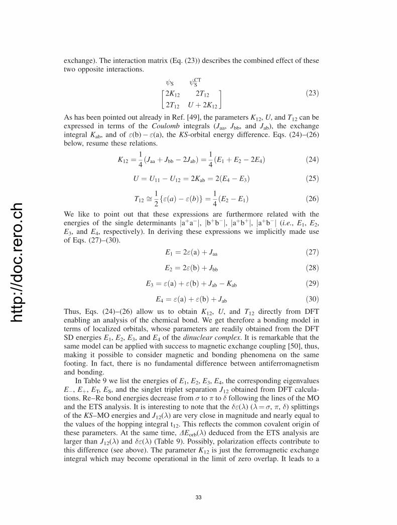
http://doc.rero.ch

exchange). The interaction matrix (Eq. (23)) describes the combined effect of thesetwo opposite interactions.

S CTS

2K12 2T12

2T12 U þ 2K12

� � ð23Þ

As has been pointed out already in Ref. [49], the parameters K12, U, and T12 can beexpressed in terms of the Coulomb integrals (Jaa, Jbb, and Jab), the exchangeintegral Kab, and of "(b)� "(a), the KS-orbital energy difference. Eqs. (24)–(26)below, resume these relations.

K12 ¼ 1

4Jaa þ Jbb � 2Jabð Þ ¼ 1

4E1 þ E2 � 2E4ð Þ ð24Þ

U ¼ U11 � U12 ¼ 2Kab ¼ 2 E4 � E3ð Þ ð25Þ

T12 ffi 1

2"ðaÞ � "ðbÞf g ¼ 1

4ðE2 � E1Þ ð26Þ

We like to point out that these expressions are furthermore related with theenergies of the single determinants jaþa�j, jbþb�j, jaþbþj, jaþb�j (i.e., E1, E2,E3, and E4, respectively). In deriving these expressions we implicitly made useof Eqs. (27)–(30).

E1 ¼ 2"ðaÞ þ Jaa ð27ÞE2 ¼ 2"ðbÞ þ Jbb ð28Þ

E3 ¼ "ðaÞ þ "ðbÞ þ Jab � Kab ð29ÞE4 ¼ "ðaÞ þ "ðbÞ þ Jab ð30Þ

Thus, Eqs. (24)–(26) allow us to obtain K12, U, and T12 directly from DFTenabling an analysis of the chemical bond. We get therefore a bonding model interms of localized orbitals, whose parameters are readily obtained from the DFTSD energies E1, E2, E3, and E4 of the dinuclear complex. It is remarkable that thesame model can be applied with success to magnetic exchange coupling [50], thus,making it possible to consider magnetic and bonding phenomena on the samefooting. In fact, there is no fundamental difference between antiferromagnetismand bonding.

In Table 9 we list the energies of E1, E2, E3, E4, the corresponding eigenvaluesE�, Eþ, ET, ES, and the singlet triplet separation J12 obtained from DFT calcula-tions. Re–Re bond energies decrease from � to � to � following the lines of the MOand the ETS analysis. It is interesting to note that the �"(�) (�¼ �, �, �) splittingsof the KS–MO energies and J12(�) are very close in magnitude and nearly equal tothe values of the hopping integral t12. This reflects the common covalent origin ofthese parameters. At the same time, DEorb(�) deduced from the ETS analysis arelarger than J12(�) and �"(�) (Table 9). Possibly, polarization effects contribute tothis difference (see above). The parameter K12 is just the ferromagnetic exchangeintegral which may become operational in the limit of zero overlap. It leads to a

33

http://doc.rero.ch

triplet (3A2) ground state in the staggered (D4d) conformation of Re2Cl82� where �

bonding is fully suppressed.

IV. Discussion and Conclusions

A chemist considers a molecule as a system of atoms and bonds, a quantumchemist treats it as a system of interacting electrons and nuclei. A possible bridgebetween these two approaches is the LCAO method which is a useful tool forcalculation and interpretation. However, a rigorous quantum theory of atomicinteractions is still lacking. Mayer’s ‘‘Chemical’’ Hamiltonian [51–53] offers adeductive approach which allows a priori of making an analysis rather thana posteriori (after having calculated the wavefunction). However, an applicationof this approach to open shell systems is still lacking. In this study, we appliedthe ETS method to TM complexes with open d-shells and compared results fromanalysis of the electron density using the Laplacian of the electron density and theelectron localization function. From this comparison we can conclude, that startingfrom ionic bonding and introducing a correction for covalency (charge transfer)and polarization yields a consistent description, thus allowing to regard the TM–ligand bond as a donor–acceptor relationship. The classical coordination bond isrelatively ionic and therefore electronic properties are focused mostly on the dn-configuration of the TM. Such a concept is highly supported by the spectroscopic

Table 9. Singlet versus triplet ground state stabilizations in eclipsed Re2Cl82� based on a two-

electron-two-center bond model within the single determinant DFT approach for �, �, and �

bondsa

�¼ � � �

E1(aþa�) �51.543 (�49.278) �51.543 (�49.278) �51.543 (�49.278)

E2(bþb�) �40.115 (�38.893) �44.029 (�42.467) �50.105 (�47.966)

E3(aþbþ) �46.287 (�44.513) �48.076 (�46.156) �51.148 (�48.919)

E4(aþb�) �46.091 (�44.285) �47.906 (�46.008) �50.833 (�48.631)

E�1(��) �51.546 (�49.283) �51.546 (�49.281) �51.609 (�49.338)

Eþ 1(����) �40.112 (�38.888) �44.025 (�42.464) �50.039 (�47.906)

ET3(���) �46.287 (�44.513) �48.076 (�46.156) �51.148 (�48.919)

ES1(���) �45.896 (�44.057) �47.736 (�45.860) �50.518 (�48.343)

J12 ¼ E� � ET �5.259 (�4.769) �3.470 (�3.125) �0.461 (�0.419)

�"(�) �5.41 �3.58 �0.704

DEorb(�) �10.633 �9.287 �0.802

K12 0.131 (0.100) 0.060 (0.068) 0.0045 (0.0045)

t12 5.714 (5.192) 3.757 (3.406) 0.719 (0.656)

U 0.391 (0.456) 0.340 (0.296) 0.630 (0.576)

a Scalar relativistic (non-relativistic, in parenthesis) spin-unrestricted ZORA calculations in D4h

symmetry with the following configurations for the Re d-orbitals (see Fig. 17) for �, � and � bonding:

(aþa�)¼ 6a1g26e1u

42b2g2; (bþb�)¼ 6a2u

26e1u42b2g

2, 6a1g26e1u

26eg2b2g

2, 6a1g26e1u

42b1u2; (aþbþ and

aþb�)¼ 6a1g16a2u

16e1u42b2g

2; 6a1g26e1u

36eg12b22g; 6a1g

26e1u42b2g

12b1u1 (a, b orbitals under consid-

eration are underlined); values of the transfer (hopping) integral t12, the Heisenberg exchange integral

(K12), and the effective transfer energy (U) are also included; Re–Re (2.236 A) and Re–Cl (2.331 A)

bond distances are obtained from LDA-DFT geometry optimizations

34

http://doc.rero.ch

behavior, which shows d–d transitions and CT-transition far apart, allowing todefine what is called to be a typical Werner type complex. Electronic absorptionand emission spectra and ESR and their interpretations using ligand field theoryhave been used to characterize electronically such compounds. These studiesrepeatedly demonstrate that ionic like dn-configurations and the many electronstates originating for them are well defined. In this sense this class of compoundsdiffers from organometallic ones, where bonding is more covalent and electroniceffects extend beyond the dn manifold to include metal s and p valence orbitals aswell.

The rather ionic character of the TM–ligand bond and the much smaller radiusof the 3d compared to the 4s orbital has led to suggest that the TM–ligand bond ismainly governed by 4s and 4p-orbitals, whereas the 3d-electrons are inactive beingmainly spectators (or spectroscopic probes) for the chemical bond [54]. Based onour analysis we cannot confirm this point. We find, that in Werner type complexes,the 3d electrons play a dominant role in bonding.

The bonding concept emerging from our analysis is illustrated in Fig. 18 takingCrF4 as an example. Starting from neutral atoms, a large amount of preparationenergy DEprep is needed to produce ionic fragments, in this case we consider Cr4þ

Fig. 18. The concept of ligand-to-metal donor–acceptor bonding energy for Werner-type complexes

of transition metals with open d-shells and its components within the ETS energy decomposition

scheme, illustrated for CrF4

35

http://doc.rero.ch

and F44� at infinite distances. Bringing these moieties from infinity to their actual

positions in the complex needs some additional energy due to Pauli (exchange)repulsion between closed shells denoted as, DEP. The sum of these twoterms defines the repulsive contribution to the bonding energy. The latter becomeslargely overcompensated by the attractive part of the bonding energy. It consistsof two components. The largest term, DEElstat, is the electrostatic (Coulomb)attraction between ions of oppositely charged ions. This is the molecular analogueof the Madelung energy in ionic crystals. Another stabilizing term, which is alsochemically the most interesting one, is the orbital relaxation energy, DEorb. It con-sists of electron charge-transfer between ions and additionally, of orbital polariza-tion of the ions due to the electrostatic field of the neighboring orbitals. The DEorb

energy can be further decomposed into symmetry species. Their variation withinclasses of closely related molecules is chemically significant and bears power ofinterpretation.

The rather ionic nature of the TM–ligand bond in Werner type complexes alsoderives from analysis based on natural bond orbitals and their extensions, i.e., thelocalized bond concept [55]. When combined with valence bond theory, thisapproach allows to locate most probable Lewis structures. Thus, sdn�1 hybrideorbitals for a MLn complex along with natural hybrid orbitals on the ligands yielda rather accurate approximation of valence electron density in many cases (up to97–99% accuracy [55]). They show that the relative participation of j4si TMorbitals to the TM–ligand bond increases with decreasing coordination number.This trend is very similar to, what we obtain presently: the inclusion of j4si yieldsstronger bonds, when going, say from CrCl6

3� to CrCl4 to CrCl2. Moreover, ionicresonance structures (such as WF3

3þðF�Þ3, W¼F double bonds, and presumablyClCl3(Cl

�)3, Cr–Cl single bonds) yield a high or dominating weight in the totalwavefunction. Also, the existence and geometries, say of CrX4 (X¼ F,Cl,Br,I)are in agreement with electron counts (4 sd3 hybride functions plus 2 unpairedelectrons¼ 6). The NBO approach is beyond the scope of the present review, seeRefs. [56–58].

The ETS method has been found to be a useful tool in analyzing the TM-bond.However, results and interpretations are biased by the choice of reference frag-ments which might differ from case to case. Thus, other methods, based on analysisof the electron density of the considered molecule can provide information for thebonding ‘‘as it is’’. Thus, the quantum theory of atoms and molecules and theelectronic localization function are valuable extensions and can assist interpreta-tions by the ETS method. We have found that the former two approaches gaininsight power for complexes of high symmetry when decomposition of the electrondensity into different irreducible representations of the molecular point group ispossible. Using such symmetry resolved Laplacians and ELF functions enabled usto show that ionic bonding in Werner type TM complexes is considerably modifiedby covalency, mostly of �-type, but turns out to be mainly ionic when looking atthe total electron density.

A more critical remark should be made when considering the quantitativeaspects of Morokuma and the closely related ETS methods. The former has beenseverely criticized from the Natural Bond Order perspective [59] as well as ongrounds of basis-set related numerical instabilities [60]. It was suggested that the

36

http://doc.rero.ch

Natural Energy Decomposition Analysis (NEDA) [61] emerges as a clear alter-native being conceptually better justified and better converging to asymptoticclassical entities. The main critique was directed to the decomposition usingnon-orthogonal fragments in the short-range region of covalent bonding, where,because of the larger overlap, conceptual ambiguities increase. It leads in the caseof ETS to inaccuracies when calculating the DEElstat term, which further propagatesinto the DEP and the DEorb terms.

In this work, we applied the ETS model using two different starting approx-imations for the reference fragments – atomic and ionic ones. We have stated that itis the ionic reference point which provides a starting point for the rather localizedd-electrons (and our analysis applies only to those cases). For localized d-electronsthe ligand–metal overlap is very small and we think that the main arguments (thebigger overlap) against the ETS method does not hold for this class of compounds.In spite of this, we feel that other energy partitioning schemes, such as the NEDAdeserve increased attention in the future. However, to our knowledge, the methodhas not yet been applied to TM compounds. We hope that the present study willstimulate some work in this direction.

Acknowledgements

The authors owe thanks to Prof. Dr. G. Frenking (Fachbereich Chemie, Philipps-Universit€aat, Marburg,

Germany) and the members of his group, and Prof. Dr. C.-W. Schl€aapfer (Fribourg) for a long standing

discussion on the problems of the chemical bond and many helpful suggestions concerning this study.

This work has been supported by the Bundesamt f€uur Forschung and Wissenschaft (Swisse) and a

COST action (D26-0013-02) within the European Science Foundation.

References

[1] Coppens P (1977) Angew Chem Int Ed Engl 16: 32

[2] Morokuma K (1977) Acc Chem Res 10: 294

[3] a) Ziegler T, Rauk A (1977) Theor Chim Acta (Berl) 46: 1; b) Bickelhaupt FM, Baerends EJ

(2000) In: Lipkowitz KB, Boyd DB (eds) Reviews in Computational Chemistry, vol 15. Wiley-

VCH, New York, chapter 1 and references cited therein

[4] Pauling L (1931) J Am Chem Soc 53: 1367

[5] Pauling L (1975) Proc Nat Acad Sci USA 72: 4200

[6] Pauling L (1976) Proc Nat Acad Sci USA 73: 274

[7] Frenking G, Fr€oohlich N (2000) Chem Rev 100: 717

[8] Glerup J, Monsted O, Sch€aaffer CE (1976) Inorg Chem 15: 1399

[9] Smith DW (1978) Structure and Bonding 35: 87

[10] a) te Velde G, Bickelhaupt FM, Baerends EJ, Fonesca Guerra C, van Gisbergen SJA, Snijders JG,

Ziegler T (2001) J Comput Chem 22: 931; b) ADF program, release ADF2004.01, web site:

http:==www.scm.com

[11] a) Bader RFW (1990) Atoms in Molecules. A quantum theory. Oxford University press, Oxford,

and references cited therein; b) Xaim-1.0 – a X11 graphical user interface to several programs

based on some aspects of the theory of atoms in molecules (EXTREME and FLOPO, interfaced

to ADF2004.01), Jos�ee Cralos Ortiz Alba and Carles Bo Jan�ee, Department de Quimica Fisica

I Inorganica Universitat Rovira I Virgili, Taragona, Spain; http:==www.quimica.urv.es=

ADF_UTIL, free domain

37

http://doc.rero.ch

[12] Becke AD, Edgecombe KE (1990) J Chem Phys 92: 5397

[13] Silvi B, Savin A (1994) Nature 371: 683

[14] Savin A, Jepsen O, Flad J, Anderson OK, Preuss H, von Schnering HG (1992) Angew Chem Int

Ed Engl 31: 187

[15] a) Kohout M (2004) Int J Quant Chem 97: 651; b) Kohout M (2004) Programs Basin and Dgrid

(interfaced to ADF), version 2.4. Max Planck Institute for Chemical Physics of Solids, Dresden,

free available from kohout@cpfs.mpg.de

[16] a) Savin A, Silvi B, Colonna F (1996) Can J Chem 74:1088; b) Noury S, Colonna F, Savin A,

Silvi B (1998) J Mol Struct 450: 59; c) Silvi B (2004) Phys Chem Chem Phys 6: 256; d) Pilme J,

Silvi B, Alikhani ME (2003) J Phys Chem A 107: 4506

[17] Jørgensen CK (1962) Absorption spectra and chemical bonding in compexes. Pergamon Press,

Oxford

[18] Cremer D, Kraka E (1984) Angew Chem Int Ed Engl 23: 627

[19] Shaik S, Maitre P, Sini G, Hiberty PC (1992) J Am Chem Soc 114: 7861

[20] Kutzelnigg W (1991) In: Maksic ZB (ed) Theoretical Models of Chemical Bonding, vol 2.

Springer, Berlin, pp 1–44

[21] Fradera X, Austen MA, Bader RFW (1999) J Phys Chem A 103: 304

[22] Silvi B, Pilme J, Fuster F, Alikhani ME (2003) In: Russo N et al. (eds) Metal Ligand Interactions.

Kluwer, pp 241–284

[23] Calatayud M, Andr�ees J, Beltran A, Silvi B (2001) Theor Chem Acc 105: 299

[24] Gillespie RJ, Noury S, Pilm�ee J, Silvi B (2004) Inorg Chem 43: 3248

[25] H€aaussermann U, Wengert S, Nesper R (1994) Angew Chem Int Ed Engl 33: 2073

[26] Santos JC, Tiznado W, Contreras R, Fuentealba P (2003) J Chem Phys 120: 1670

[27] Silvi B, Kryachko ES, Tishchenko O, Fuster F, Nguyen MT (2002) Mol Phys 100: 1659

[28] Jørgensen CK, Pappalardo R, Schmidtke H-H (1963) J Chem Phys 39: 1422

[29] Sch€aaffer CE (1968) Structure and Bonding 5: 67

[30] Figgis BN (1987) In: Wilkinson G (ed) Comprehensive Coordination Chemistry, vol 1.

Pergamon Press, Oxford, p 225

[31] Sch€oonherr T, AtanasovM, AdamskyH (2003) In: Comprehensive Coordination Chemistry, vol 2,

p 443

[32] Vanquickenborne LG, Ceulemans A (1981) Inorg Chem 20: 796

[33] Smith DW (1977) Inorg Chim Acta 22: 107

[34] Klamt A, Sch€uurrmann G (1993) J Chem Soc Perkin Trans 2, 799

[35] Pye CC, Ziegler T (1999) Theor Chem Acc 101: 396

[36] Atanasov MA, Reinen D (2004) Inorg Chem 43:1998

[37] Penka Fowe E (in preparation) PhD Thesis, Univ Fribourg

[38] Tregenna-Piggott PLW, Best SP, G€uudel HU, Weihe H, Wilson CC (1999) Solid State Chem 145:

460

[39] Tregenna-Piggott PLW, Weihe H, Bendix J, Barra A-L, G€uudel H-U (1999) Inorg Chem 38: 5928

[40] Spichiger D, Carver G, Dobe C, Bendix J, Tregenna-Piggott PLW,Meier R, Zahn G (2001) Chem

Phys Lett 337: 391

[41] Wang SG, Schwarz WHE (1998) J Chem Phys 109: 7252

[42] a) Cotton FA, Curtis NF, Johnson BFG, Robinson WR (1965) Inorg Chem 4: 326; b) Cotton FA,

Harris CB (1965) Inorg Chem 4: 330; c) Cotton FA (1965) Inorg Chem 4: 334

[43] Heitler W, London F (1927) Z f€uur Physik 44: 455

[44] Coulson CA, Fischer I (1949) Philosophical Magazine 40: 386

[45] Cotton FA, Nocera DG (2000) Accounts of chemical research 33: 483, and references cited

therein

[46] Llusar R, Beltran A, Andr�ees J, Fuster F, Silvi B (2001) J Phys Chem A 105: 9460

[47] Bursten BE, Clayton TW Jr (1994) Journal of Cluster Science 5: 157

38

http://doc.rero.ch

[48] Anderson PW (1959) Phys Rev 115: 2

[49] Hay PJ, Thibeault JC, Hoffmann R (1975) J Am Chem Soc 97: 4884

[50] Atanasov M, Daul CA (2003) Chem Phys Lett 379: 209

[51] Mayer I (1983) Int J Quantum Chem XXIII: 363

[52] Mayer I (2000) Chem Phys Lett 332: 381

[53] Mayer I (2003) Chem Phys Lett 382: 265

[54] Gerloch M, Constable EC (1994) Transition metal chemistry. The valence shell in d-block

chemistry. VCH, Weinheim New York

[55] Weinhold F, Landis CR (2001) Chemistry education: research and practice in Europe 2: 91

[56] Landis CR, Cleveland T, Firman TK (1995) J Am Chem Soc 117: 1859

[57] Landis CR, Firman TK, Root DM, Cleveland T (1998) J Am Chem Soc 120: 1842

[58] Weinhold F, Landis CR (book announced in Ref. 45)

[59] Weinhold F (2003) Angew Chem Int Ed Engl 42: 4188

[60] Cybilsky SM, Scheiner S (1990) Chem Phys Lett 166: 57

[61] Glendening ED, Steitwieser A (1994) J Chem Phys 100: 2900

39