Chemical analysis of globular star clusters: theory and ... · Chemical analysis of globular star...
173
Chemical analysis of globular star clusters: theory and observation Karin Lind M¨ unchen 2010
Transcript of Chemical analysis of globular star clusters: theory and ... · Chemical analysis of globular star...
Chemical analysis of globular starclusters: theory and observation
Karin Lind
Munchen 2010

Chemical analysis of globular starclusters: theory and observation
Karin Lind
Dissertation
an der Ludwig–Maximilians–Universitat
Munchen
vorgelegt von
Karin Lind
aus Motala, Schweden
Munchen, den 28.09.2010

Erstgutachter: Priv. Doz. Dr. Achim Weiß
Zweitgutachter: Priv. Doz. Dr. Joachim Puls
Tag der mundlichen Prufung: 13.12.2010
Contents
Zusammenfassung xiii
Summary xv
Preface xvii
1 Abundance analysis of late-type stars 11.1 The chemical composition of stars . . . . . . . . . . . . . . . . . . . . . . . 11.2 Model atmospheres . . . . . . . . . . . . . . . . . . . . . . . . . . . . . . . 21.3 LTE analysis . . . . . . . . . . . . . . . . . . . . . . . . . . . . . . . . . . 31.4 Non-LTE analysis . . . . . . . . . . . . . . . . . . . . . . . . . . . . . . . . 5
1.4.1 Atomic data . . . . . . . . . . . . . . . . . . . . . . . . . . . . . . . 61.4.2 Motivation for new calculations . . . . . . . . . . . . . . . . . . . . 71.4.3 Non-LTE effects . . . . . . . . . . . . . . . . . . . . . . . . . . . . . 7
2 Non-LTE calculations for neutral Na using improved atomic data 112.1 Astrophysical motivation . . . . . . . . . . . . . . . . . . . . . . . . . . . . 112.2 Non-LTE modelling procedure . . . . . . . . . . . . . . . . . . . . . . . . . 12
2.2.1 Structure of the model atom . . . . . . . . . . . . . . . . . . . . . . 132.2.2 Radiative transitions . . . . . . . . . . . . . . . . . . . . . . . . . . 142.2.3 Electron collisions . . . . . . . . . . . . . . . . . . . . . . . . . . . . 142.2.4 Hydrogen collisions . . . . . . . . . . . . . . . . . . . . . . . . . . . 172.2.5 Line broadening . . . . . . . . . . . . . . . . . . . . . . . . . . . . . 18
2.3 Discussion . . . . . . . . . . . . . . . . . . . . . . . . . . . . . . . . . . . . 182.3.1 Departures from LTE . . . . . . . . . . . . . . . . . . . . . . . . . . 182.3.2 The influence of collisions . . . . . . . . . . . . . . . . . . . . . . . 232.3.3 Consequences for stellar abundance analysis . . . . . . . . . . . . . 26
2.4 Conclusions . . . . . . . . . . . . . . . . . . . . . . . . . . . . . . . . . . . 28
3 Departures from LTE for neutral Li 313.1 Astrophysical motivation . . . . . . . . . . . . . . . . . . . . . . . . . . . . 313.2 Non-LTE modelling procedure . . . . . . . . . . . . . . . . . . . . . . . . . 313.3 Results . . . . . . . . . . . . . . . . . . . . . . . . . . . . . . . . . . . . . . 34
vi CONTENTS
3.4 Discussion . . . . . . . . . . . . . . . . . . . . . . . . . . . . . . . . . . . . 35
4 3D, non-LTE line formation of Na I in the Sun 41
4.1 Introduction . . . . . . . . . . . . . . . . . . . . . . . . . . . . . . . . . . . 41
4.2 Modelling procedure . . . . . . . . . . . . . . . . . . . . . . . . . . . . . . 42
4.3 Line formation in 3D . . . . . . . . . . . . . . . . . . . . . . . . . . . . . . 45
4.4 Centre-to-limb variation . . . . . . . . . . . . . . . . . . . . . . . . . . . . 46
4.5 The solar Na abundance . . . . . . . . . . . . . . . . . . . . . . . . . . . . 51
5 Globular clusters 53
5.1 Definition and basic properties . . . . . . . . . . . . . . . . . . . . . . . . . 53
5.2 Evolution of low-mass stars . . . . . . . . . . . . . . . . . . . . . . . . . . 56
5.3 Observational applications . . . . . . . . . . . . . . . . . . . . . . . . . . . 57
5.4 High-resolution spectroscopy with FLAMES . . . . . . . . . . . . . . . . . 59
5.4.1 The observational setup . . . . . . . . . . . . . . . . . . . . . . . . 59
5.4.2 Data reduction and processing . . . . . . . . . . . . . . . . . . . . . 60
5.5 Determination of stellar parameters . . . . . . . . . . . . . . . . . . . . . . 61
5.5.1 Effective temperature . . . . . . . . . . . . . . . . . . . . . . . . . . 61
5.5.2 Surface gravity . . . . . . . . . . . . . . . . . . . . . . . . . . . . . 64
6 Signatures of intrinsic Li depletion and Li-Na anti-correlation in themetal-poor globular cluster NGC 6397 65
6.1 Introduction . . . . . . . . . . . . . . . . . . . . . . . . . . . . . . . . . . . 65
6.2 Observations . . . . . . . . . . . . . . . . . . . . . . . . . . . . . . . . . . . 68
6.2.1 High and medium-high resolution spectroscopy . . . . . . . . . . . . 68
6.2.2 Stromgren photometry . . . . . . . . . . . . . . . . . . . . . . . . . 69
6.3 Analysis . . . . . . . . . . . . . . . . . . . . . . . . . . . . . . . . . . . . . 74
6.3.1 Effective temperatures and surface gravities . . . . . . . . . . . . . 75
6.3.2 Metallicity . . . . . . . . . . . . . . . . . . . . . . . . . . . . . . . . 76
6.3.3 Lithium . . . . . . . . . . . . . . . . . . . . . . . . . . . . . . . . . 79
6.3.4 Sodium . . . . . . . . . . . . . . . . . . . . . . . . . . . . . . . . . 79
6.3.5 Calcium . . . . . . . . . . . . . . . . . . . . . . . . . . . . . . . . . 80
6.4 Results . . . . . . . . . . . . . . . . . . . . . . . . . . . . . . . . . . . . . . 80
6.4.1 Li abundances . . . . . . . . . . . . . . . . . . . . . . . . . . . . . . 80
6.4.2 Lithium data from the ESO archive . . . . . . . . . . . . . . . . . . 83
6.4.3 The Li-Na anti-correlation . . . . . . . . . . . . . . . . . . . . . . . 83
6.5 Discussion . . . . . . . . . . . . . . . . . . . . . . . . . . . . . . . . . . . . 86
6.5.1 Signatures of intrinsic lithium depletion . . . . . . . . . . . . . . . . 86
6.5.2 Effects of stellar parameters and non-LTE . . . . . . . . . . . . . . 91
6.5.3 Comparison to other studies . . . . . . . . . . . . . . . . . . . . . . 91
6.5.4 Comparison to diffusion-turbulence models . . . . . . . . . . . . . . 92
6.6 Conclusions . . . . . . . . . . . . . . . . . . . . . . . . . . . . . . . . . . . 95
CONTENTS vii
7 Tracing the evolution of NGC 6397 through the chemical composition ofits stellar populations 977.1 Introduction . . . . . . . . . . . . . . . . . . . . . . . . . . . . . . . . . . . 977.2 Observations and analysis . . . . . . . . . . . . . . . . . . . . . . . . . . . 997.3 Abundance analysis . . . . . . . . . . . . . . . . . . . . . . . . . . . . . . . 101
7.3.1 O, Na, Mg, and Al . . . . . . . . . . . . . . . . . . . . . . . . . . . 1057.3.2 Nitrogen . . . . . . . . . . . . . . . . . . . . . . . . . . . . . . . . . 1097.3.3 α and iron-peak elements . . . . . . . . . . . . . . . . . . . . . . . . 1107.3.4 Neutron capture elements . . . . . . . . . . . . . . . . . . . . . . . 1127.3.5 Helium . . . . . . . . . . . . . . . . . . . . . . . . . . . . . . . . . . 113
7.4 Consequences for the evolutionary scenario . . . . . . . . . . . . . . . . . . 1167.4.1 Method . . . . . . . . . . . . . . . . . . . . . . . . . . . . . . . . . 1167.4.2 Amount of dilution between massive star ejecta and pristine gas . . 1177.4.3 Expected anti-correlations . . . . . . . . . . . . . . . . . . . . . . . 1197.4.4 He content . . . . . . . . . . . . . . . . . . . . . . . . . . . . . . . . 1227.4.5 Initial cluster mass . . . . . . . . . . . . . . . . . . . . . . . . . . . 122
7.5 Conclusions . . . . . . . . . . . . . . . . . . . . . . . . . . . . . . . . . . . 123
8 Conclusions and outlook 1298.1 The cosmological Li problem . . . . . . . . . . . . . . . . . . . . . . . . . . 1298.2 Multiple populations in globular clusters . . . . . . . . . . . . . . . . . . . 1308.3 The future of high-precision abundance analysis . . . . . . . . . . . . . . . 131
Bibliography 146
Acknowledgments 149
Curriculum Vitae 154

viii CONTENTS
List of Figures
1.1 The optical depth dependence of the mean radiation field Jν and the Planckfunction Bν for a solar atmospheric model. . . . . . . . . . . . . . . . . . . 8
1.2 Solar LTE and non-LTE curves-of-growth for one of the NaD lines (λ589.5 nm). 9
2.1 Schematic term diagram of the 23-level Na I model atom. . . . . . . . . . . 132.2 Three sample excitation cross-sections for collisions between Na I and electrons. 162.3 Comparison between rate coefficients at T = 6000K for collisional excitation
of Na I by neutral hydrogen atoms. . . . . . . . . . . . . . . . . . . . . . . 192.4 Non-LTE abundance corrections as functions of equivalent widths of selected
Na I lines. . . . . . . . . . . . . . . . . . . . . . . . . . . . . . . . . . . . . 202.5 Contour diagrams illustrating non-LTE abundance corrections. . . . . . . . 242.6 The sensitivity of Na I departure coefficients to hydrogen collisions. . . . . 252.7 Comparison with the non-LTE Na abundance corrections determined in ear-
lier studies. . . . . . . . . . . . . . . . . . . . . . . . . . . . . . . . . . . . 272.8 Comparison between temperature stratifications and curves-of-growth of Na
lines for different 1D model atmosphere codes. . . . . . . . . . . . . . . . . 29
3.1 The sensitivity of Li non-LTE abundance corrections to hydrogen collisionsfor different stellar parameters. . . . . . . . . . . . . . . . . . . . . . . . . 36
3.2 The sensitivity of Li non-LTE abundance corrections to choice of 1D modelatmosphere code. . . . . . . . . . . . . . . . . . . . . . . . . . . . . . . . . 37
3.3 Comparison of the derived Li non-LTE abundance corrections to earlierstudies. . . . . . . . . . . . . . . . . . . . . . . . . . . . . . . . . . . . . . . 38
4.1 Temperature and electron density structures of solar model atmospheres in1D and 3D. . . . . . . . . . . . . . . . . . . . . . . . . . . . . . . . . . . . 44
4.2 Solar disk centre intensity profiles of the Na I 615.4 nm line. . . . . . . . . . 454.3 Departure coefficients for Na I 3s and 3p with optical depth . . . . . . . . . 474.4 Surface images of atmospheric variables for a solar 3D radiation-hydrodynamic
simulation . . . . . . . . . . . . . . . . . . . . . . . . . . . . . . . . . . . . 484.5 Centre-to-limb variation of the equivalent widths of Na I lines. . . . . . . . 494.6 Centre-to-limb variation of solar Na I line profiles. . . . . . . . . . . . . . . 50
5.1 A schematic view of the positions of all known globular clusters in the Galaxy. 54
x LIST OF FIGURES
5.2 A zoomed in view of Fig. 5.1. . . . . . . . . . . . . . . . . . . . . . . . . . 555.3 The observed HR-diagram of NGC6397. . . . . . . . . . . . . . . . . . . . 585.4 Cross-section along the order direction of the GIRAFFE CCD decector. . . 62
6.1 (b− y)− Teff and (v − y)− Teff relations derived for NGC6397. . . . . . . . 706.2 The (b− y)0 −MV fiducial sequence. . . . . . . . . . . . . . . . . . . . . . 716.3 Histograms of the Fe I and Fe II excitation and ionisation equilibria of the
targets. . . . . . . . . . . . . . . . . . . . . . . . . . . . . . . . . . . . . . . 776.4 Example fits to the Li I 670.7 nm line and the Na I 819.4 nm line. . . . . . . 786.5 Li abundances plotted next to the observed HR diagram of NGC 6397. . . 826.6 Comparison between our observed Li data and archival data. . . . . . . . . 846.7 Li and Na abundances for dwarfs and subgiants. . . . . . . . . . . . . . . . 876.8 Bin-averaged Li abundances against absolute visual magnitude. . . . . . . 886.9 Bin-averaged Li abundances against effective temperature. . . . . . . . . . 896.10 Comparison of Li abundance trends with luminosity to stellar structure mod-
els with atomic diffusion and mixing. . . . . . . . . . . . . . . . . . . . . . 936.11 Same as in in Fig 6.10 but with effective temperature as the reference axis. 94
7.1 The targeted red giant branch stars are marked with black bullets in theV − (v − y) diagram of NGC 6397. . . . . . . . . . . . . . . . . . . . . . . 100
7.2 Sample UVES spectra and best-fit synthetic model. . . . . . . . . . . . . . 1027.3 Elemental abundances of all targets. . . . . . . . . . . . . . . . . . . . . . 1037.4 Non-LTE Na abundance variation with effective temperature in NGC6397. 1057.5 Na abundance histograms. . . . . . . . . . . . . . . . . . . . . . . . . . . . 1067.6 Na, Mg, Al, and O abundances. . . . . . . . . . . . . . . . . . . . . . . . . 1087.7 Comparison between abundances of RGB stars in NGC6397 and halo field
stars. . . . . . . . . . . . . . . . . . . . . . . . . . . . . . . . . . . . . . . . 1097.8 Correlation between Na-abundance and colour index cy on the red giant
branch. . . . . . . . . . . . . . . . . . . . . . . . . . . . . . . . . . . . . . . 1117.9 Model preditions for the Li and Na abundances for unevolved stars in
NGC 6397. . . . . . . . . . . . . . . . . . . . . . . . . . . . . . . . . . . . . 1187.10 Model predictions for the O–Na and O–Al anti-correlations for red giant stars.1207.11 Expected anti-correlation between helium mass fraction and [O/Na . . . . 121
List of Tables
2.1 Line data for the ten Na I lines considered in the detailed spectrum synthesis. 15
3.1 Wavelengths, oscillator strengths, and broadening data for the two consid-ered Li I lines. . . . . . . . . . . . . . . . . . . . . . . . . . . . . . . . . . . 33
3.2 Non-LTE abundance corrections and equivalent widths for the Li I λ =670.7 nm line. . . . . . . . . . . . . . . . . . . . . . . . . . . . . . . . . . . 35
3.3 Non-LTE abundance corrections and equivalent widths for the Li I λ =610.3 nm line. . . . . . . . . . . . . . . . . . . . . . . . . . . . . . . . . . . 37
4.1 The solar Na abundance derived from five Na I lines with different modellingassumptions. . . . . . . . . . . . . . . . . . . . . . . . . . . . . . . . . . . . 52
6.1 FLAMES observations. . . . . . . . . . . . . . . . . . . . . . . . . . . . . 716.2 Photometry and effective temperatures. . . . . . . . . . . . . . . . . . . . . 726.3 Iron lines measured in the UVES spectrum of one red giant branch star. . . 736.3 Continued. . . . . . . . . . . . . . . . . . . . . . . . . . . . . . . . . . . . . 746.4 Adopted stellar parameters, equivalent widths, and Li, Na, and Ca abun-
dances. The full table can be retrieved from CDS/Vizier. . . . . . . . . . . 81
7.1 Mean abundances and abundance dispersions compared to literature valuesfor NGC 6397. . . . . . . . . . . . . . . . . . . . . . . . . . . . . . . . . . . 104
7.2 Stellar parameters for #5644 and #14565 derived assuming a normal-starhydrogen and helium composition. . . . . . . . . . . . . . . . . . . . . . . . 114
7.3 Iron mass fractions derived for #5644 and #14565, assuming different massfractions of helium . . . . . . . . . . . . . . . . . . . . . . . . . . . . . . . 115
7.4 Line list with reference to the adopted oscillator strength. . . . . . . . . . . 1247.4 Continued. . . . . . . . . . . . . . . . . . . . . . . . . . . . . . . . . . . . . 1257.4 Continued. . . . . . . . . . . . . . . . . . . . . . . . . . . . . . . . . . . . . 1267.5 Individual star abundances and stellar parameters. . . . . . . . . . . . . . 1277.6 Continued. . . . . . . . . . . . . . . . . . . . . . . . . . . . . . . . . . . . . 128

xii LIST OF TABLES
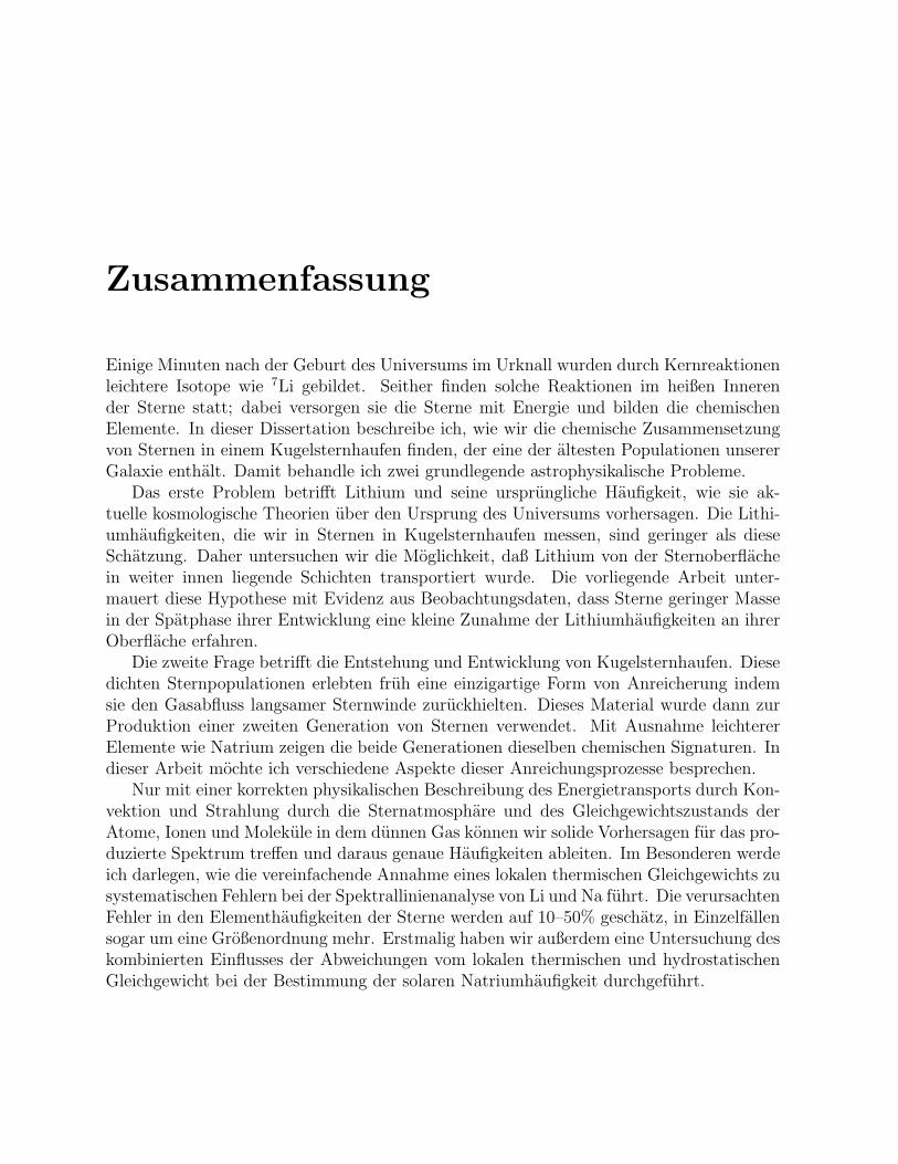
Zusammenfassung
Einige Minuten nach der Geburt des Universums im Urknall wurden durch Kernreaktionenleichtere Isotope wie 7Li gebildet. Seither finden solche Reaktionen im heißen Innerender Sterne statt; dabei versorgen sie die Sterne mit Energie und bilden die chemischenElemente. In dieser Dissertation beschreibe ich, wie wir die chemische Zusammensetzungvon Sternen in einem Kugelsternhaufen finden, der eine der altesten Populationen unsererGalaxie enthalt. Damit behandle ich zwei grundlegende astrophysikalische Probleme.
Das erste Problem betrifft Lithium und seine ursprungliche Haufigkeit, wie sie ak-tuelle kosmologische Theorien uber den Ursprung des Universums vorhersagen. Die Lithi-umhaufigkeiten, die wir in Sternen in Kugelsternhaufen messen, sind geringer als dieseSchatzung. Daher untersuchen wir die Moglichkeit, daß Lithium von der Sternoberflachein weiter innen liegende Schichten transportiert wurde. Die vorliegende Arbeit unter-mauert diese Hypothese mit Evidenz aus Beobachtungsdaten, dass Sterne geringer Massein der Spatphase ihrer Entwicklung eine kleine Zunahme der Lithiumhaufigkeiten an ihrerOberflache erfahren.
Die zweite Frage betrifft die Entstehung und Entwicklung von Kugelsternhaufen. Diesedichten Sternpopulationen erlebten fruh eine einzigartige Form von Anreicherung indemsie den Gasabfluss langsamer Sternwinde zuruckhielten. Dieses Material wurde dann zurProduktion einer zweiten Generation von Sternen verwendet. Mit Ausnahme leichtererElemente wie Natrium zeigen die beide Generationen dieselben chemischen Signaturen. Indieser Arbeit mochte ich verschiedene Aspekte dieser Anreichungsprozesse besprechen.
Nur mit einer korrekten physikalischen Beschreibung des Energietransports durch Kon-vektion und Strahlung durch die Sternatmosphare und des Gleichgewichtszustands derAtome, Ionen und Molekule in dem dunnen Gas konnen wir solide Vorhersagen fur das pro-duzierte Spektrum treffen und daraus genaue Haufigkeiten ableiten. Im Besonderen werdeich darlegen, wie die vereinfachende Annahme eines lokalen thermischen Gleichgewichts zusystematischen Fehlern bei der Spektrallinienanalyse von Li und Na fuhrt. Die verursachtenFehler in den Elementhaufigkeiten der Sterne werden auf 10–50% geschatz, in Einzelfallensogar um eine Großenordnung mehr. Erstmalig haben wir außerdem eine Untersuchung deskombinierten Einflusses der Abweichungen vom lokalen thermischen und hydrostatischenGleichgewicht bei der Bestimmung der solaren Natriumhaufigkeit durchgefuhrt.

xiv
Summary
A few minutes after the Big Bang that created our Universe, nucleosynthesis reactionsforged some lighter isotopes, including 7Li. Ever since then, such reactions have takenplace in the hot stellar interiors, providing the stars with the energy to shine and formingall chemical elements necessary for life as we know it. In this thesis I describe how wehave inferred the chemical composition of stars in a globular cluster, hosting one of theoldest stellar populations in our Galaxy, in order to address two fundamental astrophysicalproblems.
The first problem is related to lithium, and the prediction of its primordial abundancefrom present cosmological theories of how the Universe was born. The Li abundances thatwe measure in the envelopes of globular cluster stars are lower than this estimate and weinvestigate the possibility that Li has been drained from the stellar surfaces. This thesispresents observational evidence that low-mass stars experience a small increase in theirsurface Li abundances during the course of their late phases of evolution, supporting thishypothesis.
The second question is related to the formation and evolution of globular clusters.It appears that these dense stellar environments early underwent a unique form of self-enrichment, by retaining the gas outflow from slow stellar winds. The material was thenincorporated into a second stellar generation with identical chemical signatures to the first,except for a handful of lighter elements, including sodium. I here discuss several aspectsof this stellar pollution process.
Only with a correct physical description of the radiative and convective energy transportthrough the stellar atmosphere, and the equilibrium state of the atoms, ions and moleculesthat form the tenuous gas, can we make solid predictions of the emergent spectrum andderive accurate abundances. In particular, I discuss how the simplifying assumption of localthermal equilibrium give rise to systematic errors in the analysis of Li and Na spectral lines,commonly mis-estimating the elemental abundances in stars by 10–50%, and in certaincases considerably more. Moreover, we have for the first time investigated the combinedinfluence from departures from local thermal equilibrium and hydro-static equilibrium inthe determination of the solar Na abundance.

xvi
Preface
The dissertation consists of eight chapters of which two are introductory, five containjournal articles that have been published or are being prepared for publication, and one(Chapter 8) summarises the main conclusions and discusses future prospects.
Chapter 1 introduces the basic concepts and physical assumptions behind modellingof stellar atmospheres and abundance analysis of late-type stars. This is followed bythree chapters that present theoretical investigations of lithium (3) and sodium abundancedetermination (2 and 4). I conducted essentially all the practical work presented in thesechapters myself, with minor assistance by the listed co-authors. This included e.g. theassembly of new improved model atoms for Na and Li, setting up and executing an efficientnumerical procedure for comprehensive 1D, non-LTE calculations, and conducting severaltests on my own and my co-authors’ initiatives, in order to interpret the results. Toperform the 3D, non-LTE investigation presented in Chapter 4, I also took significant partin adapting the presented code to accurate abundance analysis and testing its performanceto that end. The field of combined 3D, non-LTE analyses of elemental abundances is indeedin its infancy and my work has significantly contributed to its development.
Chapter 5 describes fundamental properties of globular clusters and outlines the stepsinvolved in processing of high-resolution spectroscopic data and the basic concepts of stel-lar parameter determination. Chapters 6 and 7 contain observational investigations ofglobular cluster stars and extensive discussions on the astrophysical gain of the presentedanalyses. The work has been based on data collected during two observing runs at the ESOVery Large Telescope at Paranal Observatory, Chile. I was the Principal Investigator ofone of the observing programmes and thus had the main responsibility for the applicationfor observing time and preparation of the observational procedure for this run. Further, Iwas responsible for the data reduction and processing of all observational data, the deter-mination of stellar parameters, the assembly of the adopted line lists, and the developmentof techniques to efficiently perform large-scale abundance analysis through spectrum syn-thesis and equivalent width measurements. I also took the leading part in interpreting theresults and placing them in a larger context. With the exception of Sect. 4.1, 6.1, and 7.4I am the main author of all sections presented in this work.

xviii
Chapter 1
Abundance analysis of late-type stars
The chemical composition of a star’s outermost layer is imprinted onto its electromagneticspectrum, in particular through the strengths of spectral lines. By constructing a modelof the temperature and density stratification of the atmosphere and use radiative transferto predict the spectrum of emitted radiation, we may constrain the chemical abundancesof different elements in the atmosphere. Depending on the level of sophistication of themodelling procedure and the desired accuracy of the result, this can be anything from arelatively straightforward to a highly complex process.
The following chapter introduces the reader to some of the basic assumptions andterminology involved in traditional abundance analysis of so called late-type stars. Thiscollective term refers to stars that have masses similar to the Sun and thus share severalother characteristics as well, such as size, luminosity, surface temperature and gravity, ata given evolutionary phase. Here we are mainly concerned with late-type stars of spectralclasses F, G, and K (see e.g. Gray, 2005), and luminosity classes III (giants), IV (subgiants)and V (dwarfs). These stars have masses M = 0.5 − 1.6 M and main sequence (MS)luminosities L = 0.1− 6.5 L
1.
1.1 The chemical composition of stars
A ’normal’ star consists of roughly 90% hydrogen and 10% helium particles. All otherspecies are referred to as ’metals’ and their total number density is typically <∼ 0.1%.Even though they are insignificant in numbers, the metals have a profound importancefor many aspects of the evolution of individual stars and galaxies, not to mention planetformation. The vast majority of all heavier elements that exist in the Universe today haveindeed been synthesised inside stars and partly returned to the interstellar gas during thelate phases of stellar evolution. By studying the chemical composition of stars in differentenvironments and ages, we can trace this cosmic recycling process.
The abundance of metals in a star is usually specified on a logarithmic scale relative tohydrogen, such that A(X) = log(ε(X)) + 12 = log(N (X)/N (H)) + 12, where N(X) is the
1The quoted values are adopted from “A dictionary of Astronomy” (www.encyclopedia.com)
2 1. Abundance analysis of late-type stars
number density of element X. This notation will be used throughout the text. Further, it iscommon to use the iron abundance relative to the Sun as a measure of the total ’metallicity’of the star, using a bracket notation: [Fe/H] = log(N (Fe)/N (H))− log(N (Fe)/N (H)). Astar with [Fe/H]= −2 thus has 100 times less iron compared to the Sun, and the same (orsimilar) scaling factor is usually applied to all other elements.
Individual elemental abundances in stars are specified either in absolute numbers, A(X),or using the bracket notation [X/Fe]. The latter notation indicates how much an element isdeficient or in excess with respect to the solar composition, again with iron as the referenceelement. As an example, inter-mediate mass elements with even atomic number (O, Ne,Mg, Si, S, Ar, Ca, Ti) are usually assumed to be enhanced in metal-poor stars, such that[X/Fe] > 0. This is referred to as α-enhancement.
1.2 Model atmospheres
The most common physical assumptions behind atmospheric modelling of late-type starsare (see e.g. Kurucz, 1970; Gray, 2005; Gustafsson et al., 2008):
• hydro-static equilibrium, where gravity is balanced by the thermal and turbulentpressure of the gas and by radiation pressure.
• a one-dimensional, plane-parallel or spherically symmetric, geometry.
• energy transport via radiation and convection, with the efficiency of convective fluxparametrised with so called ’mixing length theory’.
• local thermodynamic equilibrium (LTE).
These assumptions are all more or less realistic approximations of the actual physicalstate of the atmosphere. During recent decades it has been possible to relax the three firstassumptions, and 3D, hydro-dynamical models (e.g. Stein & Nordlund, 1998; Nordlundet al., 2009; Vogler et al., 2005; Freytag et al., 2010), simulating the convective motions inthe atmospheres from first principles, are becoming increasingly realistic and suitable forabundance analysis (see further Chapter 4). Still, much work remains to be done in thisdirection before 3D models can be used for quantitative spectroscopy of a large number ofstars, and the observational applications that are described in Chapters 2 and 3 are basedon traditional 1D models (Gustafsson et al., 2008). Section 4 explores 3D line formationfor the specific case of the Sun.
A traditional 1D model is characterised by a set of stellar parameters:
• the effective temperature, Teff , which gives an indication of the typical temperaturesin the photospheric layers from which the bulk of the radiation is emitted. It is relatedto the total flux, F , emitted by the star via Stefan-Boltzmann’s law of black-bodyradiation, F = σT 4
eff .
1.3 LTE analysis 3
• the (logarithmic) surface gravity, log(g), where g = GM/R2, M is the mass of thestar, R is the stellar radius, and G is Newton’s constant of gravity.
• the chemical composition, usually indicated by [Fe/H].
• the stellar mass (only for spherically symmetric models).
• the ’microturbulence’ ξt, which is a parametrised way of accounting for the pressureand thus additional line broadening caused by (small-scale) turbulent gas motions.This velocity parameter is an artifact of the approximate treatment of convection instatic 1D models and becomes obsolete with 3D hydro-dynamical simulations.
• a set of additional parameters describing the convective flux, of which the mostimportant is α = l/Hp, where l is a characteristic length scale mixed by convectionand Hp is the pressure scale height.
In the theoretical investigations of LTE departures for Li and Na that are described infollowing two chapters we use an extensive grid of 1D models. The effective temperatureof the grid ranges from 4000K to 8000K, the logarithmic surface gravity from 1.0 to5.0 (cgs units, g given in [cm s−2]), the metallicity from solar to [Fe/H]= −3.0, and themicroturbulence from 1 to 5 km/s. This parameter space covers metal-rich and metal-poor dwarf and giant stars, mainly of spectral type FGK, and the calculations are thusapplicable to stars in all types of Galactic populations (see further Chapter 5).
Note that when discussing different depths in the photosphere, it is common to use theoptical depth, τ , at 500 nm as the reference scale, rather than the geometrical distance.The continuum radiation emitted at this reference wavelength has its largest contributionfrom a depth where τ500 = 1. In solar-type stars, continuum regions at shorter wavelengthstypically probe slightly deeper layers and vice verse for longer wavelengths. The fluxemitted at wavelengths where spectral lines are located receives part or most contribution(depending on line strength) from shallower depths, i.e. τ500 < 1. Also note that all modelsthat are discussed here neglect magnetic fields, and are not reproducing the chromospherictemperature rise.
1.3 LTE analysis
The assumption of LTE in the computation of model atmospheres simplifies the problemdramatically, as all excitation and ionisation fractions of atoms and molecules depend onlyon the local electron temperature and density in LTE. The task of finding the numberdensities of different excitation and ionisation stages for a given chemical composition,and thus obtain the monochromatic opacity at each point in the atmosphere, becomescomputationally manageable. Further, model atmospheres computed in LTE successfullypredict the absolute fluxes of solar-type stars (with the possible exception of the far ultra-violet regime, e.g. Allende Prieto et al. 2003) and the centre-to-limb variation of thecontinuum intensity (using 3D models, see Pereira et al. 2009b).
4 1. Abundance analysis of late-type stars
In LTE, the relative number populations of different excitation levels of a given speciesfollow the Boltzmann distribution:
Nj
Ni
=gj
gi
e−∆E/kT , ∆E = Ej − Ei (1.1)
In this expression, gi, is the statistical weight and Ei the excitation energy of level i.The only atmospheric variable in this equation is thus temperature. Similarly, the relativeionisation fractions are given by the Saha equation:
Nn+1
Nn
=(2πmekT )3/2
Neh3
2un+1
un
e−I/kT (1.2)
Here, Nn is the total number density of a given atom or ion, Nn+1 is the number densityof the next ionisation stage and Ne the electron density. I is the ionisation potential, andun =
∑i gie
−Ei/kT is the partition function of species n. The other variables have their usualmeaning. The ionisation fraction at different depths of the atmosphere is thus dependentboth on the surface gravity and the chemical composition through Ne, as well as on thetemperature.
Once the level populations of all elements are specified, the radiation transport canbe solved for at any given wavelength and a model of the emitted flux from the star canbe produced (spectrum synthesis) and compared to the observed spectrum. A simplifiedapproach is to compare the integrated spectral line strengths, the so called equivalentwidth, defined as:
Wλ =∫
line(1− Fλ/Fc)dλ (1.3)
Fλ is the wavelength-dependent flux and Fc the continuum flux (the equivalent widthcan also be defined from the intensity, as in Chapter 4). Wλ is thus measured in units ofdistance, commonly in pm (= 10−12 m) or mA (= 10−13 m). It is not always appropriate oreven possible to compare the equivalent widths of model and observations, especially notin cases where lines are blended (overlapping) with lines from other species.
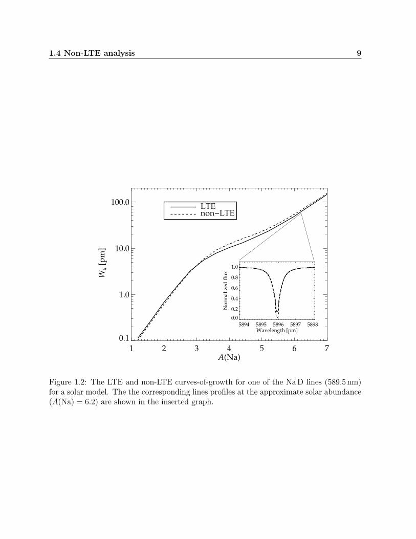
Weak, single lines have approximate Gaussian shapes and are in general the mostsuitable for abundance analysis purposes (not considering observational challenges). Oneof the main reasons is that in this regime, the line strength has the strongest dependence(linear) on the number density of atoms residing in the lower level involved in the bound-bound transition (Fig. 1.2). Depending on the temperature and density structure of theatmosphere, the excitation and ionisation equilibrium changes, and different spectral linesmay thus be suitable as abundance indicators for different stars (Sect. 2.3.3).
To compute a synthetic spectrum of a line, given the LTE assumption and the contin-uous background opacity, one must know the transition probability (oscillator strength f)for the bound-bound radiative transition that is producing the spectral line. In addition,atomic data for line broadening are necessary to determine its width and shape. Broaden-ing of spectral lines is caused by the finite life time of atomic states (natural or radiativebroadening) and by perturbations of the energy levels by surrounding neutral particles
1.4 Non-LTE analysis 5
(van der Waals-broadening, mainly due to H I) and charged particles (Stark broadening,mainly due to electrons).
1.4 Non-LTE analysis
Modelling that relaxes the assumption of LTE is usually referred to simply as ’non-LTE’or statistical equilibrium (SE), which in practise means that the level populations of allpossible excitation and ionisation states for a given element are assumed not to change withtime. To obtain the correct level populations, one must know the rates of radiative andcollisional transitions between the different states. The main complexity of the problemarises because the rates of radiative excitation and ionisation depend on the radiationfield, while the radiative transport through the atmosphere cannot be solved for withoutexplicit knowledge of the level populations. This calls for an iterative procedure, solvingsimultaneously for the equations of statistical equilibrium (Eq. 1.4) and radiative transfer(Eq. 1.5). Numerical solutions to this problem for multi-level atoms are described in e.g.Mihalas (1978); Rybicki & Hummer (1991); Scharmer & Carlsson (1985).
dNi
dt=∑j 6=i
NjPji −Ni
∑j 6=i
Pij = 0 (1.4)
Here Pij = Rij + Cij is the total transition rate from level i to j, including radiativerates and collisional rates. Cij is simply determined by the collisional cross-section andthe frequency of collisions, whereas Rij is dependent on the transition probabilities forphoton absorption and emission, as well as on the profile-averaged mean intensity Jφ
ν0=
1/2∫∞0
∫+1−1 Iνφ(ν−ν0)dµdν. In this expression, µ = cosθ, where θ is the angle between the
ray and the normal direction and φ is the normalised line profile. The specific intensity isfound through the transport equation in plane-parallel geometry (see e.g. Rutten 2003 fora derivation of this equation):
µdIν
dτν
= Sν − Iν (1.5)
Sν is the monochromatic source function, which represent the local addition of radiation,as defined from the opacity and emissivity of the gas. In LTE, Sν = Bν , where Bν is thePlanck function, simplifying the problem tremendously. In non-LTE, the source functiondepends on the relevant level populations of all species contributing opacity at the specificwavelength.
It is beyond the power of current supercomputers to produce full non-LTE model atmo-spheres for late-type stars, with a self-consistent treatment of the vast number of possibleatomic and molecular transitions. Still, efforts have been made in the direction of im-plementing a non-LTE treatment including at least tens of thousands lines for the mostimportant opacity sources in atmospheric modelling of late-type stars (Hauschildt et al.,1999; Short & Hauschildt, 2003, 2005). Such non-LTE atmospheric modelling has found
6 1. Abundance analysis of late-type stars
that the ultra-violet fluxes as well as the temperatures in the outermost layers may besignificantly affected by non-LTE, especially for giant stars.
However, even if a full non-LTE treatment is not yet possible, hybrid techniques can beextremely useful. In abundance analysis of late-type stars, a common assumption is thatthe element of interest is a ’trace element’, i.e. the LTE departures of the level populationof the element do not significantly change the atmospheric structure. It is thus possible toestablish the statistical equilibrium of this element for a given atmospheric structure andbackground LTE opacity, and then use the non-LTE level populations in the computationof the synthetic spectrum. Indeed, it is inconsistent to only allow for LTE departuresof one element at the time, and it hinges critically on the assumption that the modelstructure is accurately established with the LTE assumption. The success of such hybridnon-LTE approaches for hydrogen and helium in the computation of model atmospheresfor hotter dwarfs of spectral type O and B, may give some confidence of the method (Nieva& Przybilla, 2007). In Chapters 2 and 3 we adopt the trace-element modelling techniquefor Li I and Na I and show the impact on abundance analysis of these two elements.
In a general simplification, it is true that LTE is a good approximation in dense plasmas,when the collisional rates dominate the radiative rates. In stellar atmospheres, this meansthat the LTE assumption is most likely to break down in shallow layers, where the densityis low. This is another reason why weak spectral lines, formed deep in the photosphere, areto be preferred as abundance indicators. Also note that the level populations of minorityatoms or ions can be severely affected by a small perturbation in the overall ionisationequilibrium. Therefore, LTE is usually appropriate for majority species like Li II and Na II(which cannot be used for abundance work, due to the lack of visible spectral lines), butmay be a poor approximation for the neutral atoms.
1.4.1 Atomic data
To set up the statistical equilibrium equations for an element requires immensely moreatomic data than in the LTE case. To compute the radiative rates, Rij, between alllevels i and j of the system, the corresponding oscillator strengths and photo-ionisationcross-sections are needed. In addition, the cross-sections for collisional excitation andionisation must be known for all relevant colliding species, to obtain Cij. In late-typestars, collisions with free electrons are the most frequent, due to their high thermal speed.However, collisions with neutral hydrogen, which is the most abundant particle, may alsobe important. Collisions with all other species are in all likelihood too rare to be of anysignificance.
Experimental data of radiative and collisional transition probabilities do exist, butusually only for strong, key transitions. Theoretical calculations are thus necessary toprovide data in sufficient quantities. As discussed in detail for Na in Sect. 2.2, such the-oretical methods may be of varying quality. Generally, the largest uncertainties affectingthe non-LTE calculations in stellar atmospheres are collisional cross-sections, especially forcollisions with hydrogen atoms (e.g. Asplund, 2005). As described in Barklem et al. (2003)and Sect. 2.2.4, recent quantum mechanical calculations of cross-sections for collisions with
1.4 Non-LTE analysis 7
hydrogen have significantly improved the situation for Li and Na and reliable model atomscan now be constructed. In our non-LTE study of Na, we have put extra emphasis onassessing how much the remaining uncertainties in collisional rates influence the statisti-cal equilibrium, considering also improved calculations for collisional cross-sections withelectrons.
1.4.2 Motivation for new calculations
The non-LTE analyses presented in Chapters 2 and 3 were triggered by our studies of thedetailed chemical composition of globular cluster stars (see Chapters 6 and 7). Only byinvesting time to establish a reliable modelling procedure could we obtain high-precisionabundances for Li and Na, with important implications for the formation and evolution ofthese stellar populations, the physics of stellar interiors, and the primordial nucleosynthesisof Li. Literature searches convinced us for the need of new non-LTE analyses for severalreasons.
For Li, existing studies (Carlsson et al., 1994; Pavlenko & Magazzu, 1996; Takeda& Kawanomoto, 2005) did not cover the needed stellar parameter ranges with a denseenough model grid, to ensure reliable interpolation. Second, new quantum mechanicaldata for collisional cross-sections with neutral hydrogen had previously been implementedonly for a handful of stars (Barklem et al., 2003; Asplund et al., 2003). These studieshad shown that the level populations of Li I are significantly affected by charge transferreactions, specifically mutual neutralisation and ion-pair production (Li∗+H←→ Li+ +H−),which therefore were implemented in our Li I model atom. Third, the LTE departures aresensitive to the atmospheric structure, and we thus found it important to implement themost up-to-date models in our calculations. For Na, the calculations of new quantummechanical rates for collisions with both electrons and hydrogen atoms were the maintriggers, as their influence on the statistical equilibrium of Na had never been investigated.
We thus computed 1D, non-LTE calculations for neutral Li and Na for a large stellargrid. The given non-LTE abundance corrections can be interpolated to arbitrary stellar-parameter combinations within the covered grid and will thus serve useful for Li and Naabundance analyses with a variety of applications, such as those mentioned in Sect. 2.1 andSect. 3.1 and described in detail in Chapters 6 and 7. Chapter 4 is of a more exploratorynature, describing a combined 3D, non-LTE investigation of Na I line formation and therebyaddressing the shortcomings of 1D modelling. These results that are not directly applicableto globular cluster stars, but are specific to the Sun. We plan to extend our 3D, non-LTEwork to cover a larger stellar parameter space in the future.
1.4.3 Non-LTE effects
When calculating the level populations through statistical equilibrium equations, the spec-tral lines can become stronger or weaker compared to the LTE approximation. As describedin Sect. 2.3.1 this depends critically on the departure coefficients, βx = Nx/N
∗x , of the upper
level (u) and lower (l) level of the transition, where N∗x is the population found in LTE.
8 1. Abundance analysis of late-type stars
−3 −2 −1 0 1τ500
10−6
10−5
10−4
[erg
s−
1 cm
−2 H
z−1 ]
3p
n=7
n=12
BνJν
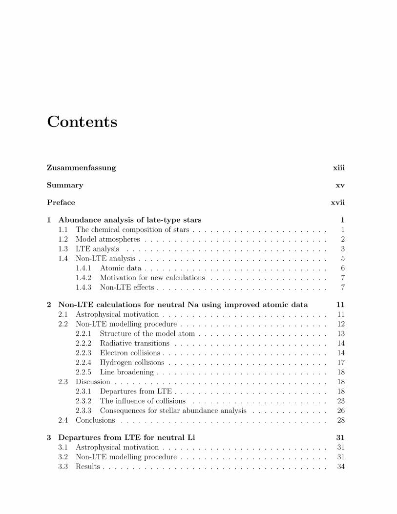
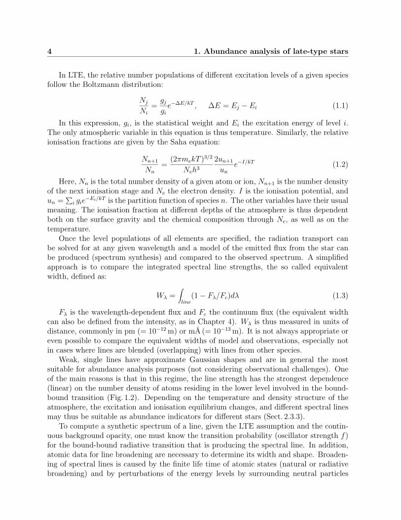
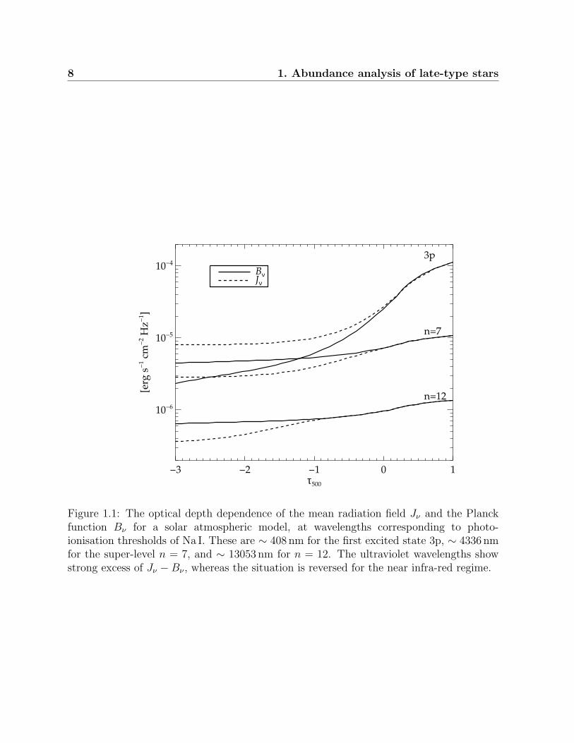
Figure 1.1: The optical depth dependence of the mean radiation field Jν and the Planckfunction Bν for a solar atmospheric model, at wavelengths corresponding to photo-ionisation thresholds of Na I. These are ∼ 408 nm for the first excited state 3p, ∼ 4336 nmfor the super-level n = 7, and ∼ 13053 nm for n = 12. The ultraviolet wavelengths showstrong excess of Jν −Bν , whereas the situation is reversed for the near infra-red regime.
1.4 Non-LTE analysis 9
1 2 3 4 5 6 7A(Na)
0.1
1.0
10.0
100.0
Wλ
[pm
]
LTEnon−LTE
5894 5895 5896 5897 5898Wavelength [pm]
0.0
0.2
0.4
0.6
0.8
1.0
No
rmal
ized
flu
x
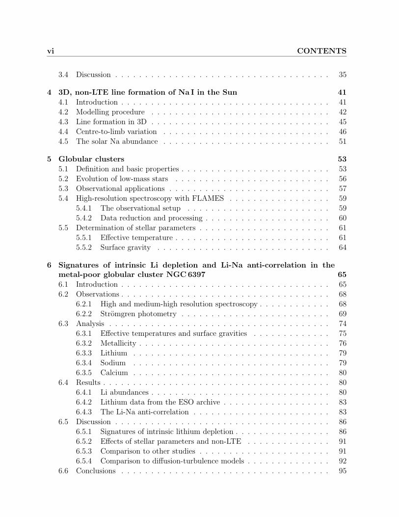
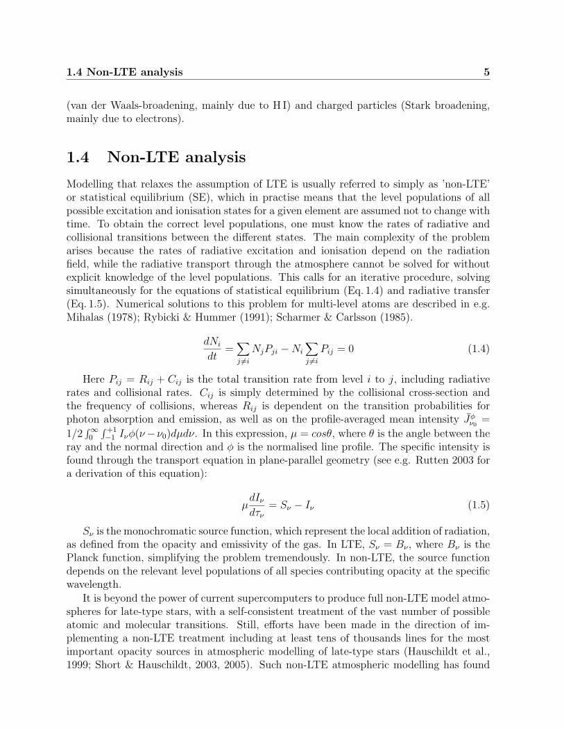
Figure 1.2: The LTE and non-LTE curves-of-growth for one of the NaD lines (589.5 nm)for a solar model. The the corresponding lines profiles at the approximate solar abundance(A(Na) = 6.2) are shown in the inserted graph.
10 1. Abundance analysis of late-type stars
βl determines the change of line opacity, whereas βu/βl determines the change in the linesource function compared to LTE. If the departures are such that βl > 0 and βu/βl < 0,both effects tend to strengthen the spectral line in non-LTE, and vice verse.
In LTE, the ionisation fractions of different ions fulfil the Saha equation (Eq. 1.2),whereas in non-LTE, the ionisation balance is determined by the strength of the radiationfield at influential photo-ionisation continua. In general, Jν is in excess of Bν in the ultra-violet and part of the optical wavelength regime, whereas the roles are reversed in thenear-infra red. As will be described in more detail in the following chapters, the ionisationequilibria of Li and Na are set by the competing effects of over-ionisation (i.e. the photo-ionisation rates are higher than in LTE, due to the Jν − Bν excess) from the first excitedstates, whose photo-ionisation thresholds lie in the ultra-violet, and over-recombination tohigher excited states. This is illustrated in Fig. 1.1. The strength of Jν is model dependent,especially on the atmospheric temperature gradient, such that the ionisation equilibriumis somewhat shifted over the grid.
In addition to the perturbed ionisation balance, the radiation fields in the spectrallines themselves influence the statistical equilibrium in non-LTE. This connection is espe-cially clear for the resonance line transitions of Li I (2s-2p) and Na I (3s-3p), whose sourcefunctions behave similarly to a two-level atom (this is also a good approximation for thestrongest subordinate transitions, Li I 2p–3d and Na I 3p–3d). In particular, the line sourcefunctions are set directly by the profile-averaged mean intensity Jφ
ν0(see further Sect. 2.3.1).
As a result, the size of the LTE departures are very much dependent on the strengths ofthe lines themselves.
Clearly, the non-LTE modelling procedure has a much greater complexity and theresults depend on the accuracy of atomic data for a large number of transitions. However,one must bear in mind that the LTE result is recovered in the strong-collision limit andis thus only an extreme version of non-LTE. The LTE assumption inevitably leads to asystematic bias, be it small or large, that we should strive to investigate for all species.As an example, Fig. 1.2 illustrates the different curves-of-growth, i.e. line strength as afunction of total elemental abundance, established with LTE and non-LTE modelling ofthe Na I line at 589.5 nm in the Sun.
Chapter 2
Non-LTE calculations for neutral Nausing improved atomic data
The following chapter contains a slightly modified version of an article that was submit-ted to Astronomy & Astrophysics in September 2010 (Lind, Asplund, Barklem, & Belyaev).
2.1 Astrophysical motivation
Sodium has established itself as an important tracer of Galactic chemical evolution and nu-merous investigations of the Na abundances of late-type stars, residing in different regionsof the Galaxy, have been conducted (see e.g. Takeda et al., 2003; Gehren et al., 2006; An-drievsky et al., 2007, and Chapter 7). Na is mainly synthesised during hydrostatic carbonburning in massive stars, in the reaction 12C(12C,p)23Na. As pointed out by Woosley &Weaver (1995), the production is dependent on the available neutron excess through sec-ondary reactions, which implies metal-dependent yields. In addition, there is a productionchannel via proton capture reactions, 22Ne(p,γ)23Na (Denisenkov & Denisenkova, 1990).The latter, so called NeNa-cycle, occurs when temperatures are high enough for H-burningthrough the CNO-cycle, e.g. in the cores or H-burning shells of inter-mediate mass andmassive stars.
Abundance studies of late-type stars in the thin disk show an increase from solar topositive [Na/Fe] ratios at super-solar metallicities, while thin and thick disk stars slightlybelow solar metallicities rather form a decreasing trend (Edvardsson et al., 1993; Reddyet al., 2003; Bensby et al., 2003; Shi et al., 2004). Relying exclusively on weak lines forthe analysis, LTE has been proved a reasonable approximation in this metallicity regime.For metal-poor stars the situation is different, especially in cases where the strong Na I Dresonance lines at 588.9/589.5 nm are the only available abundance indicators. As shownby Takeda et al. (2003) and Gehren et al. (2006), [Na/Fe] ratios are slightly sub-solar(−0.1...− 0.5) in metal-poor stars in the thick disk and the halo, in the metallicity range[Fe/H]= −3.0... − 1.0. This deficiency is only recovered through non-LTE analysis, since
12 2. Non-LTE calculations for neutral Na using improved atomic data
LTE investigations tend to overestimate the abundances, sometimes by more than 0.5 dex(see Sect. 2.3.1). Further, almost solar values result from non-LTE analysis of extremelymetal-poor stars below [Fe/H] < −3.0, where LTE analysis at least of giants rather resultsin positive ratios (Cayrel et al., 2004; Andrievsky et al., 2007). Finally, Nissen & Schuster(2010) found evidence for systematic Na abundance differences of order 0.2 dex betweenα-poor and α-rich halo stars, with important implications for the presumably separateorigin of these two Galactic components. To place all Galactic stellar populations on anabsolute Na abundance scale to the same and better precision, non-LTE is clearly required.
In globular clusters, Na is of particular interest, since the large over-abundances of thiselement, compared to field stars of similar metallicities, imply a chemical evolution scenariothat is specific to these dense stellar systems (see further Chapter 7). By detailed mappingof the Na abundance and its correlating behaviour with similar-mass and lighter elementswe may distinguish between stars formed in different formation episodes in globular clustersand eventually identify the elusive self-enrichment process that so efficiently polluted thestar-forming gas with the nucleosynthesis products of hot H-burning through the CNO-cycle and the related NeNa- and MgAl-chains (i.e. enhancement of N, Na, and Al, anddepletion of C, O, and Mg, see e.g. Carretta et al. 2009a and Chapter 7).
2.2 Non-LTE modelling procedure
We use the code MULTI, version 2.3 (Carlsson, 1986, 1992) to solve simultaneously thestatistical equilibrium and radiative transfer problems in a plane-parallel stellar atmo-sphere. Na is considered a trace element, neglecting feedback effects from changes in itslevel populations on the atmospheric structure. The LTE assumption is used for all otherspecies in the computation of background continuum and line opacity. A simultaneouslycomputed line-blanketed radiation field is thus used in the calculation of photo-ionisationrates.
The modelling procedure and model atmosphere grid are the same as described in Lindet al. (2009a). A grid of ∼ 400 1D, LTE, opacity-sampling, marcs model atmospheres(Gustafsson et al., 2008) is used in the analysis. The models span Teff = 4000...8000K,log g = 1.0...5.0, [Fe/H] = 0.0...− 3.0. Sodium abundances vary from [Na/Fe] = −2...2, insteps of 0.2 dex. The highest effective temperature is 5500K for models with log g = 1.0,6500K for log g = 2.0, 7500K for log g = 3.0, and 8000K for log g ≥ 4.0. For models withlog g ≥ 3.0, we adopted a microturbulence parameter ξt = 1.0 km s−1 and ξt = 2.0 km s−1,and for models with log g ≤ 3.0, we adopted ξt = 2.0 km s−1 and ξt = 5.0 km s−1. All modelshave standard composition, i.e. with scaled solar abundances according to Grevesse et al.(2007), plus 0.4 dex enhancement of alpha-elements in all metal-poor models ([Fe/H] ≤−1.0).
We define a non-LTE correction for each abundance point as the difference betweenthe LTE sodium abundance and the non-LTE abundance that corresponds to the sameequivalent width. Corrections are given for equivalent widths in the range 0.01− 100 pm.The equivalent width is obtained by numerical integration over the line profile, considering
2.2 Non-LTE modelling procedure 13
2S 2Po 2D 2Fo
0
1
2
3
4
5
En
erg
y [
eV]
3s
3p3/2
4s
3d 4p
5s 4d 4f 5p
6s 5d 5fg 6p 6d 6fgh
3p1/2
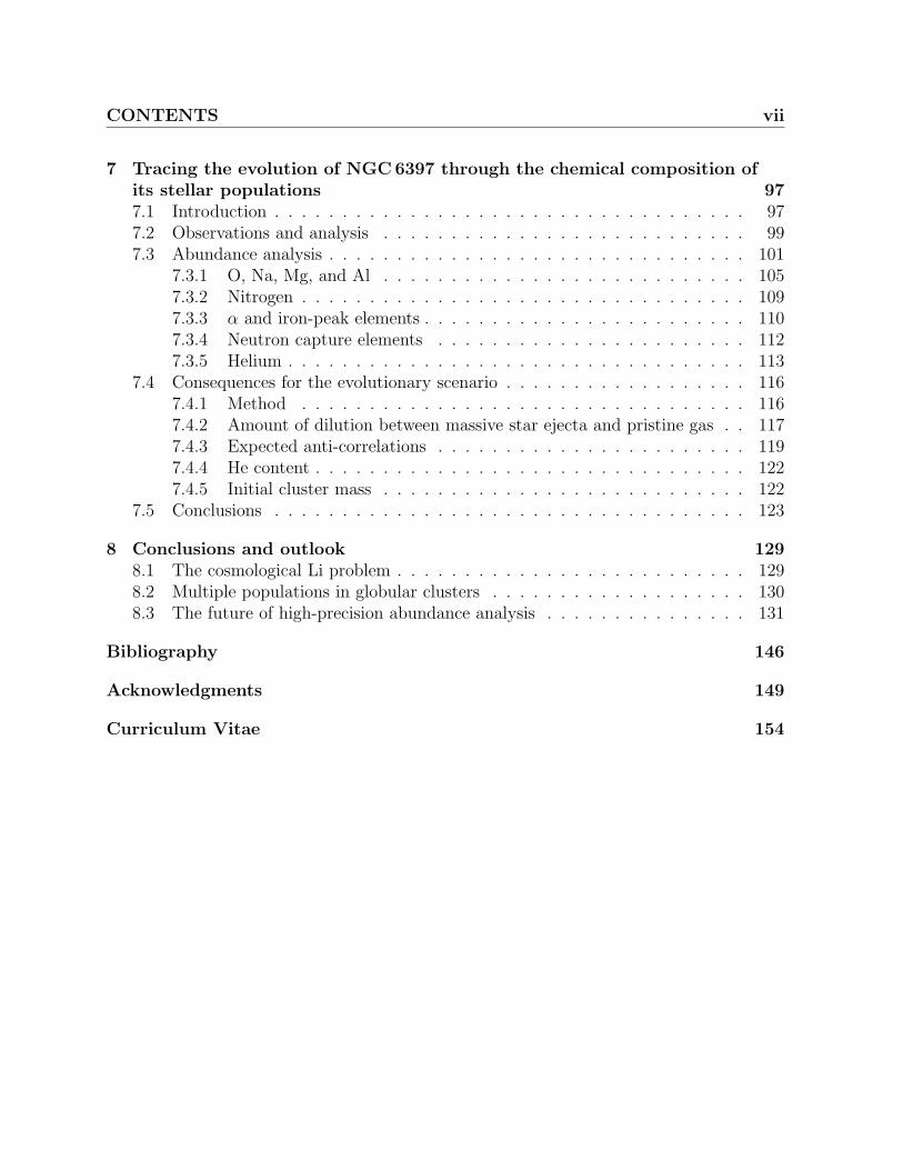
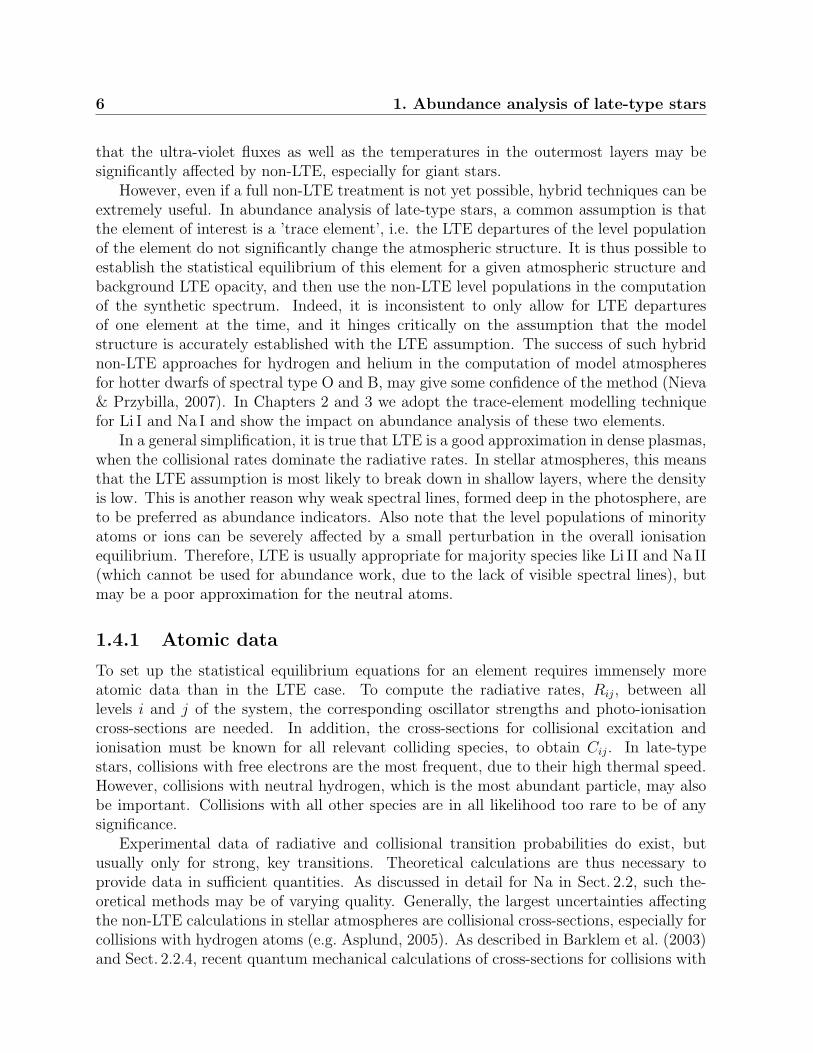
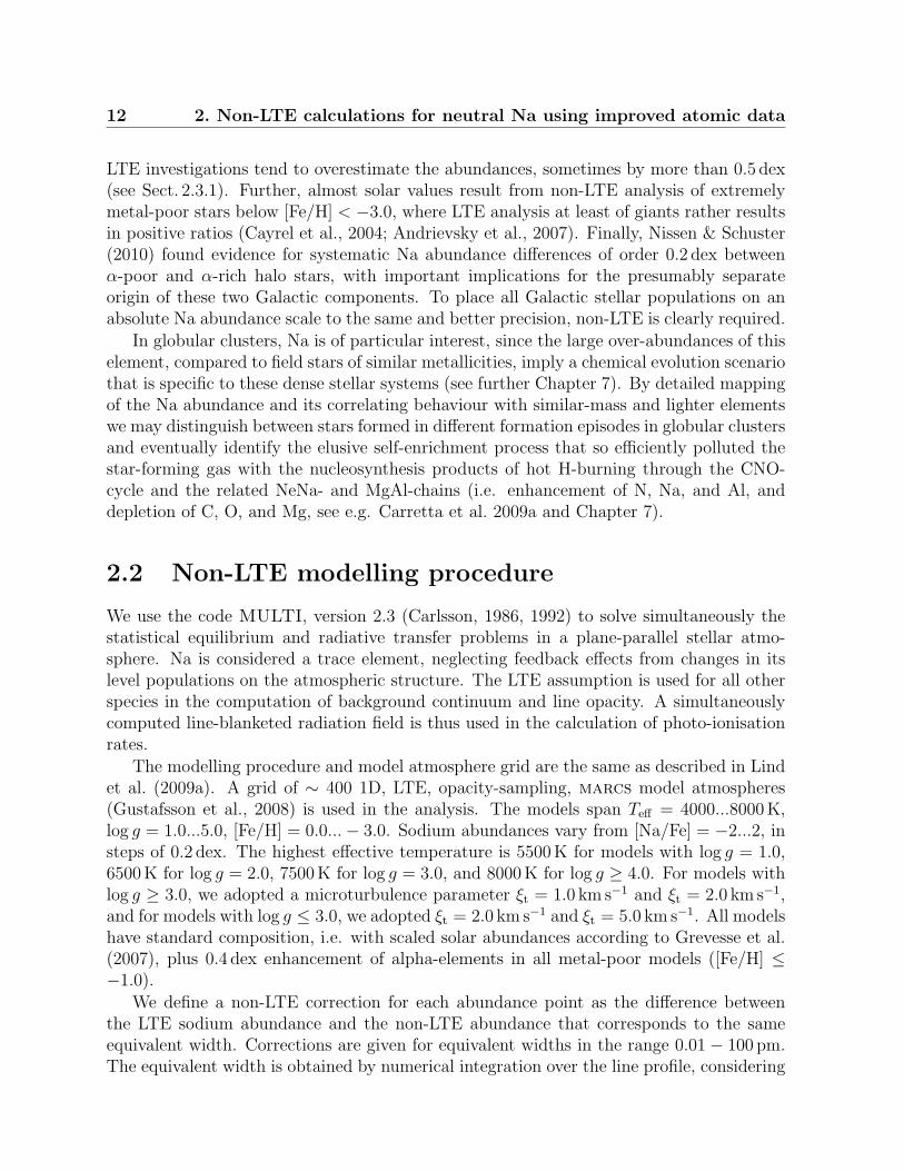
Figure 2.1: Schematic term diagram of the 23-level Na I model atom. The dashed linemarks the ground state of Na II. The highest level considered in Na I is n = 12.
a spectral region that extends ±(0.3−3) nm from the line centre, depending on the typicalline strength.
2.2.1 Structure of the model atom
The model atom we have constructed for Na consists of 22 energy levels of Na I, plus theNa II continuum (see Fig. 2.1). The energy levels are coupled via radiative transitions andvia collisional transitions with electrons and neutral hydrogen. Experimentally measuredenergies are taken from the recent compilation by Sansonetti (2008) (for highly excitedstates isoelectronic fitting is used). Since we are not concerned with modelling the detailedstructure of highly excited levels, we have collapsed all sub-levels for n = 7−12 into super-levels. The fine-structure components of the 3p level are accounted for in the statisticalequilibrium calculations, by treating 3p1/2 and 3p3/2 as separate, collisionally coupledlevels1. In addition, the fine-structure components of the 3p–3d and 3p–4d transitions, aswell as the hyper-fine structure components of the 3s–3p1/2 and 3s–3p3/2 transitions, areaccounted for by computing the line profile as a linear combination of the sub-components
1Accounting for the fine-structure of the 3p level simplifies the numerical procedure, while also predict-ing correct line formation depths for the individual lines Mashonkina et al. (e.g. 2000).

14 2. Non-LTE calculations for neutral Na using improved atomic data
(see Table 2.1).The collisional transition probabilities have been computed for the 3p level, not for its
fine-structure components. To calculate these we assume that the ionisation and excitationrates of the sub-levels are equal to that of the collapsed level. We further assume that thede-excitation rates to 3s scale with the statistical weights, i.e. the de-excitation rate from3p3/2 is twice as large as from 3p1/2, and the sum of the rates is equal to that of thecollapsed level. The collisional cross-section for electron impact excitation between the twofine-structure levels has been estimated with Seaton’s impact parameter method (Seaton,1962). We note that the detailed rates are not important for the non-LTE problem.
2.2.2 Radiative transitions
In total, 166 allowed bound-bound radiative transitions are included, adopting where pos-sible oscillator strengths from the ab initio calculations of C. Froese Fischer 2. For mostremaining transitions, we use the calculated transition probabilities by K.T. Taylor, aspart of the Opacity Project 3. The two sets of f -values are typically within 3% agreement,for the strongest, most important transitions. For the Na I D lines, accurate experimentaldata exist, and we adopt the values listed in the NIST data base4 (see Table 2.1).
Photo-ionisation cross-sections for levels with l ≤ 4 are drawn from the TOP base(computations by K.T.Taylor). For the highly excited collapsed levels we adopt hydrogeniccross-sections.
2.2.3 Electron collisions
Cross-sections for collisional excitation by electrons can be estimated using general semi-classical recipes such as the Born approximation, which is, however, known to overestimatethe cross-sections at low impact energies Park (e.g. 1971). Those near-threshold energiesare most relevant for stellar atmospheres, hosting electrons with typical kinetic energies oforder 1 eV. Seaton (1962) tried to rectify the Born cross-sections by modifying the transi-tion probability for low impact parameters, thus accounting for strong coupling betweenstates, which was previously neglected (the so called impact parameter approximation).Another approach is to empirically adjust the Born rates, to reach better agreement withexperimental data, which has been done by van Regemorter (1962) and Park (1971). Inthe absence of alternatives, non-LTE applications have long had to rely almost exclusivelyon such simple semi-empirical formulae.
Nowadays, much more rigorous quantum mechanical calculations can be performed forsimple atoms like Na. Igenbergs et al. (2008) presented new convergent close-coupling(CCC) calculations for excitation and ionisation of neutral Na by electron impact, givinggood agreement with experimental data when available (e.g. with the measurements by
2Multi-configuration Hartree-Fock computations (MCHF). http://www.vuse.vanderbilt.edu/∼cff/mchf collection/
3TOP base, http://legacy.gsfc.nasa.gov/topbase4http://physics.nist.gov/PhysRefData/ASD/index.html
2.2 Non-LTE modelling procedure 15
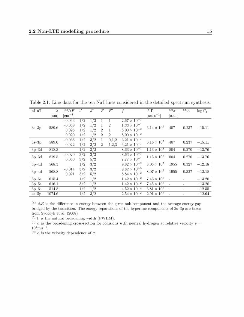
Table 2.1: Line data for the ten Na I lines considered in the detailed spectrum synthesis.
nl–n’l’ λ (a)∆E J J ′ F F ′ f (b)Γ (c)σ (d)α log C4
[nm] [cm−1] [rad s−1] [a.u. ]
3s–3p 589.6
-0.033 1/2 1/2 1 1 2.67× 10⁻²
6.14× 10⁷ 407 0.237 −15.11-0.039 1/2 1/2 1 2 1.33× 10⁻¹
0.026 1/2 1/2 2 1 8.00× 10⁻²
0.020 1/2 1/2 2 2 8.00× 10⁻²
3s–3p 589.0 -0.036 1/2 3/2 1 0,1,2 3.21× 10⁻¹
6.16× 10⁷ 407 0.237 −15.110.022 1/2 3/2 2 1,2,3 3.21× 10⁻¹
3p–3d 818.3 1/2 3/2 8.63× 10⁻¹ 1.13× 10⁸ 804 0.270 −13.76
3p–3d 819.5 -0.020 3/2 3/2 8.63× 10⁻²
1.13× 10⁸ 804 0.270 −13.760.030 3/2 5/2 7.77× 10⁻¹
3p–4d 568.3 1/2 3/2 9.82× 10⁻² 8.05× 10⁷ 1955 0.327 −12.18
3p–4d 568.8 -0.014 3/2 3/2 9.82× 10⁻³
8.07× 10⁷ 1955 0.327 −12.180.021 3/2 5/2 8.84× 10⁻²
3p–5s 615.4 1/2 1/2 1.42× 10⁻² 7.43× 10⁷ - - −13.203p–5s 616.1 3/2 1/2 1.42× 10⁻² 7.45× 10⁷ - - −13.203p–6s 514.8 1/2 1/2 4.52× 10⁻³ 6.81× 10⁷ - - −12.554s–5p 1074.6 1/2 3/2 2.54× 10⁻² 2.91× 10⁷ - - −12.64
(a) ∆E is the difference in energy between the given sub-component and the average energy gapbridged by the transition. The energy separations of the hyperfine components of 3s–3p are takenfrom Sydoryk et al. (2008)(b) Γ is the natural broadening width (FWHM).(c) σ is the broadening cross-section for collisions with neutral hydrogen at relative velocity v =104m s−1.(d) α is the velocity dependence of σ.
16 2. Non-LTE calculations for neutral Na using improved atomic data
0 2 4 6 8 10 12Energy [eV]
1
10
100
1000
Ex
cita
tio
n c
ross
sec
. [a 02
]
3s−3p
3s−4s
4p−4f
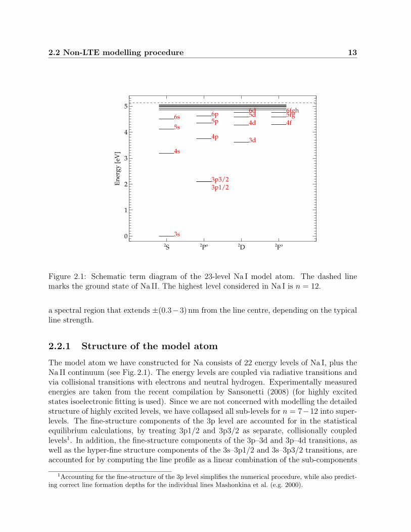
Figure 2.2: Three sample excitation cross-sections for collisions between Na I and electrons.The black solid lines represent R-matrix calculations (Gao et al., 2010; Feautrier et al., inpreparation) and the red dashed lines represent the analytical fitting functions derivedby Igenbergs et al. (2008). The transitions are marked with labels next to the energythresholds.
2.2 Non-LTE modelling procedure 17
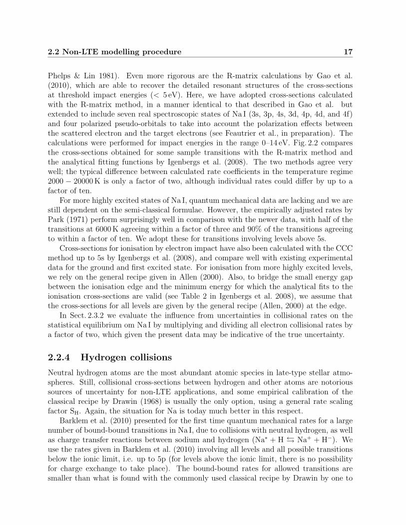
Phelps & Lin 1981). Even more rigorous are the R-matrix calculations by Gao et al.(2010), which are able to recover the detailed resonant structures of the cross-sectionsat threshold impact energies (< 5 eV). Here, we have adopted cross-sections calculatedwith the R-matrix method, in a manner identical to that described in Gao et al. butextended to include seven real spectroscopic states of Na I (3s, 3p, 4s, 3d, 4p, 4d, and 4f)and four polarized pseudo-orbitals to take into account the polarization effects betweenthe scattered electron and the target electrons (see Feautrier et al., in preparation). Thecalculations were performed for impact energies in the range 0–14 eV. Fig. 2.2 comparesthe cross-sections obtained for some sample transitions with the R-matrix method andthe analytical fitting functions by Igenbergs et al. (2008). The two methods agree verywell; the typical difference between calculated rate coefficients in the temperature regime2000 − 20000K is only a factor of two, although individual rates could differ by up to afactor of ten.
For more highly excited states of Na I, quantum mechanical data are lacking and we arestill dependent on the semi-classical formulae. However, the empirically adjusted rates byPark (1971) perform surprisingly well in comparison with the newer data, with half of thetransitions at 6000K agreeing within a factor of three and 90% of the transitions agreeingto within a factor of ten. We adopt these for transitions involving levels above 5s.
Cross-sections for ionisation by electron impact have also been calculated with the CCCmethod up to 5s by Igenbergs et al. (2008), and compare well with existing experimentaldata for the ground and first excited state. For ionisation from more highly excited levels,we rely on the general recipe given in Allen (2000). Also, to bridge the small energy gapbetween the ionisation edge and the minimum energy for which the analytical fits to theionisation cross-sections are valid (see Table 2 in Igenbergs et al. 2008), we assume thatthe cross-sections for all levels are given by the general recipe (Allen, 2000) at the edge.
In Sect. 2.3.2 we evaluate the influence from uncertainties in collisional rates on thestatistical equilibrium om Na I by multiplying and dividing all electron collisional rates bya factor of two, which given the present data may be indicative of the true uncertainty.
2.2.4 Hydrogen collisions
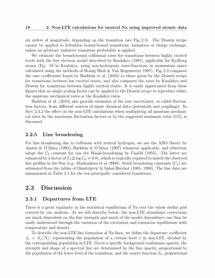
Neutral hydrogen atoms are the most abundant atomic species in late-type stellar atmo-spheres. Still, collisional cross-sections between hydrogen and other atoms are notorioussources of uncertainty for non-LTE applications, and some empirical calibration of theclassical recipe by Drawin (1968) is usually the only option, using a general rate scalingfactor SH. Again, the situation for Na is today much better in this respect.
Barklem et al. (2010) presented for the first time quantum mechanical rates for a largenumber of bound-bound transitions in Na I, due to collisions with neutral hydrogen, as wellas charge transfer reactions between sodium and hydrogen (Na∗ + H ←→ Na+ + H−). Weuse the rates given in Barklem et al. (2010) involving all levels and all possible transitionsbelow the ionic limit, i.e. up to 5p (for levels above the ionic limit, there is no possibilityfor charge exchange to take place). The bound-bound rates for allowed transitions aresmaller than what is found with the commonly used classical recipe by Drawin by one to
18 2. Non-LTE calculations for neutral Na using improved atomic data
six orders of magnitude, depending on the transition (see Fig. 2.3). The Drawin recipecannot be applied to forbidden bound-bound transitions, ionisation or charge exchange,unless an arbitrary radiative transition probability is applied.
We estimate the bound-bound collisional rates for transitions between highly excitedlevels with the free electron model described by Kaulakys (1991), applicable for Rydbergatoms (Eq. 18 in Kaulakys, using non-hydrogenic wave-functions in momentum spacecalculated using the methods of Hoang Binh & Van Regemorter 1997). Fig. 2.3 comparesthe rate coefficients found by Barklem et al. (2010) to those given by the Drawin recipefor transitions between low excited states, and also compares the rates by Kaulakys andDrawin for transitions between highly excited states. It is easily appreciated from thesefigures that no single scaling factor can be applied to the Drawin recipe to reproduce eitherthe quantum mechanical rates or the Kaulakys rates.
Barklem et al. (2010) also provide estimates of the rate uncertainty, so called fluctua-tion factors, from different sources of input chemical data (potentials and couplings). InSect. 2.3.2 the effect on the non-LTE calculations when multiplying all quantum mechani-cal rates by the maximum fluctuation factors or by the suggested minimum value (0.5), isdiscussed.
2.2.5 Line broadening
For line broadening due to collisions with neutral hydrogen, we use the ABO theory byAnstee & O’Mara (1995); Barklem & O’Mara (1997) whenever applicable, and otherwiseadopt the C6 constant for van der Waals-broadening by Unsold (1955). The latter areenhanced by a factor of 2 (∆ log C6 ≈ 0.8), which is typically required to match the observedline profiles in the Sun (e.g. Mashonkina et al. 2000). Stark broadening constants (C4) areestimated from the tables of Dimitrijevic & Sahal-Brechot (1985, 1990). The line data aresummarised in Table 2.1 for the ten principally considered transitions.
2.3 Discussion
2.3.1 Departures from LTE
There is a great regularity in the statistical equilibrium of Na over the whole stellar gridcovered by our analysis. As we will describe below, the non-LTE abundance correctionsare much dependent on the line strength and much of the model dependence can thus beeasily understood through the variation of the excitation and ionisation equilibrium withtemperature and density.
To describe the non-LTE line formation of Na lines, we define the departure coefficientβx = Nx/N
∗x , representing the population of a certain level x in non-LTE, divided by
the corresponding population in LTE. Given a specific background continuum opacity, thestrength and shape of a spectral line are determined by the line opacity, proportional tothe population of the lower level of the transition, and the source function Sν , proportional
2.3 Discussion 19
0 1 2 3 4 5∆E [eV]
100
102
104
106
108
RS
H=
1.0/R
Bar
kle
m+
0.0 0.2 0.4 0.6 0.8∆E [eV]
100
102
104
106R
SH
=1.
0/R
Kau
lak
ys+
Figure 2.3: Comparison between rate coefficients at T = 6000K for collisional excitationof Na I by neutral hydrogen atoms. Only optically allowed transitions are shown with thex-axis representing the energy of the transition. Top: The ratio between the unscaledDrawin formula and the free electron model of Kaulakys (1991) for transitions betweenhighly excited states. Bottom: The ratio between the unscaled Drawin formula and thequantum mechanical calculations by Barklem et al. (2010) for transitions between levelsup to 5s.
20 2. Non-LTE calculations for neutral Na using improved atomic data
0.1 1.0 10.0Wλ [pm]
−0.6
−0.4
−0.2
0.0
A(N
a)−
A(N
a)L
TE
5889818356826160
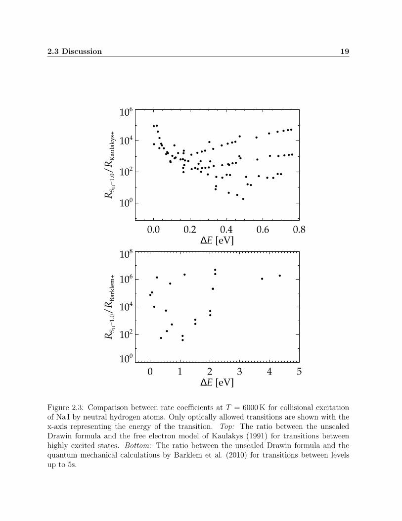
Teff = 6500K, log g = 4.5, [Fe/H] = −2, ξ = 2.0 km/s
Figure 2.4: Non-LTE abundance corrections as functions of equivalent widths of selectedNa I lines for a model with Teff = 6500K, log g = 4.5, [Fe/H] = −2, and ξt = 2.0 km/s.The leftmost value of each line (this point falls outside of the plot for all lines except thesolid) corresponds to [Na/Fe] = −1.6, and the rightmost to [Na/Fe] = +1.6.
2.3 Discussion 21
to the population ratio between the upper and lower level5. Lifting the assumption of LTE,both the line formation depth and source function may change and thus alter the strengthand shape of the spectral line.
The strong Na I D doublet lines at 588.9/589.5 nm are commonly used in abundancestudies of metal-poor stars. In fact, in certain cases (warm, metal-poor dwarfs) they arethe only lines that are sufficiently strong. The doublet originates from the resonance linetransition between the ground state (3s) and the two fine structure components of thefirst excited state (3p1/2 and 3p3/2). As a general rule, the line source function resemblesperfectly that of a pure scattering line in a two-level atom, i.e. to a very good approximationSl = Jφ at all depths, where Jφ is the profile-averaged mean intensity. This merely reflectsthe fact that for these lines, the photon absorption and emission rates strongly dominate thecollisional rates and all interactions with other levels, including the continuum. Althoughin principle, for a two-level atom, Sl = (1−εν)Jφ+ενBν , the probability for true absorption,εν , is very close to zero at shallow depths where Jφ departs from Bν , so the approximationof a pure scattering line holds at all depths.
The ratio between the population of the upper and lower level is therefore always set bythe mean intensity, and, for a specific line strength, this is correctly established with a sim-ple two-level atom. However, the actual population of the ground level, which governs theline opacity and typical formation depth of the line, is underestimated when more highlyexcited levels of Na I are neglected. As described by Bruls et al. (1992), a number of highexcitation levels and a ladder of high-probability transitions connecting these with lowerexcitation levels, must be established to obtain the correct populations. This is needed be-cause the first and second excited state have photo-ionisation thresholds in the ultra-violet,where the radiation field exceeds the Planck function (Jν > Bν), pushing the ionisationbalance to over-ionisation of Na I. The situation is reversed for more highly excited levelssince their photo-ionisation thresholds lie in the near infra-red regime, where the radiationfield rather is sub-thermal (see Fig. 1.1). This ionisation/recombination picture has beendescribed previously by Takeda et al. (2003) and Mashonkina et al. (2000).
We can now qualitatively understand the non-LTE formation, starting with the Na Iresonance lines. When either line is weak, it will obviously have small influence on itsown radiation field. Therefore, Jν − Bν > 0, as is the case for neighbouring continuumregions. This is governed by the temperature gradient, which determines how rapidlyBν decreases with optical depth. At these wavelengths, the gradient is steep enough toproduce a Jν − Bν excess and, consequently, a line source function that is stronger thanin LTE (βu/βl > 1). This tends to weaken the resonance lines compared to LTE. On theother hand, the ionisation balance of Na I is always shifted to over-recombination in theline-forming regions. The ground state of Na I is thus over-populated compared to LTE(βl > 1) and the combined effect is a moderate line strengthening. The resulting abundancecorrections for the resonance lines are always minor, |∆A| < 0.1 dex at line strengths below5 pm. However, the lines are only this weak in extremely metal-poor stars.
As the line strength increases towards saturation in any given model, Jν drops, and
5Neglecting stimulated emission, the line source function Sl is directly given by Sl/Bν = βu/βl
22 2. Non-LTE calculations for neutral Na using improved atomic data
the line source function becomes weaker than in LTE. This is naturally accompanied by adecrease in the excitation rate. Also the ionisation rates drop with increasing abundanceas the photo-ionising radiation field weakens. This allows recombination from the Na IIreservoir, and all levels of Na I are increasingly over-populated. The combination of largerline opacity and a weaker source function produce significant line strengthening in non-LTE,with negative abundance corrections as a result. This behaviour is illustrated in Fig. 2.4for a metal-poor dwarf. We note that even if the statistical equilibrium is not necessarilypushed further from LTE, the abundance corrections become larger and larger as the linesaturates, simply because the abundance sensitivity to equivalent width is small in thisregime. With further strengthening, the line enters onto the damping part of the curve-of-growth with the development of broad wings. Since photons from a wider frequency rangethen are able to excite the atoms, the excitation rate actually increases again, lesseningthe over-population in deep layers. The abundance sensitivity to line strength also startsto increase again, so the abundance corrections, as we define them here, reach a minimumvalue when the line is fully saturated (see Fig. 2.4) and then become less negative withhigher abundance, although such strong lines are hardly suitable for accurate abundanceanalysis through equivalent width measurements. Line profile analysis especially of thewings is more appropriate, but that is not addressed here.
Even if the two-level approximation holds true only for the resonance lines, the sub-ordinate transitions (with 3p as lower level), show a very similar behaviour. At low linestrength each line has a ’plateau’ of close-to-constant, small abundance corrections, be-coming increasingly negative as the line saturates around 20 pm. This general behaviourwith line strength has been discovered previously e.g. by Takeda et al. 2003. The strongestsubordinate transitions, 3p–3d at 818.3/819.4 nm, follow an almost identical behaviour asthe resonance lines, but are offset to more negative corrections. The latter is due to theshallower temperature gradient with continuum optical depth in the near infra-red wave-lengths, producing a Jν − Bν deficiency in the line, and a source function that is weakerthan in LTE also when the lines are very weak.
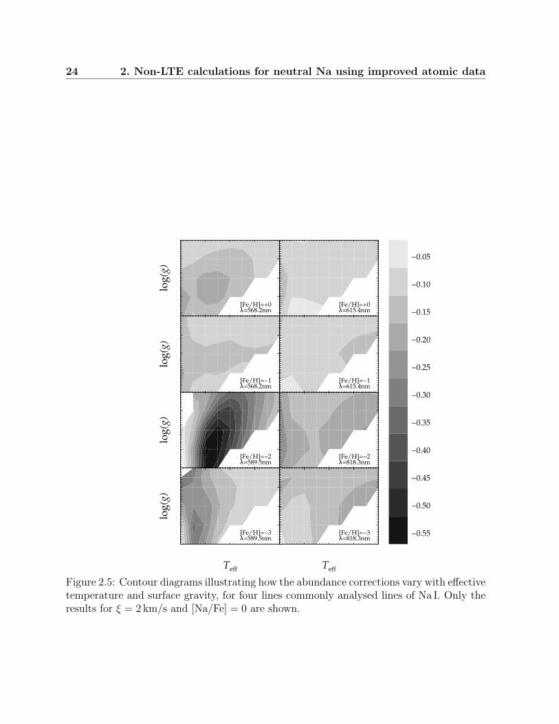
Naturally, the abundance corrections at a given line strength are still somewhat modeldependent. For saturated lines, the corrections are more negative for hotter models, andmodels with lower surface gravity, whereas the metallicity dependence seems almost neg-ligible. Fully un-saturated lines (below 5 pm) almost always have corrections in the range−0.1...− 0.2 dex.
As a curiosity, we note the very close resemblance in the non-LTE line formation ofsodium and the lighter alkali atom lithium, whose departures from LTE have been describede.g by Lind et al. (2009a) and Carlsson et al. (1994). There are many striking similaritiesbetween the two elements, especially in the shape of the abundance correction curves.Differences mainly arise from the higher degree of over-ionisation of Li, which in turn isa direct result of the larger photo-ionisation rate from the first excited state of Li I (2p),compared to Na I (3p). The abundance corrections at low line strengths thus tend to besomewhat higher, even positive, for Li (over-ionisation causes under-population of Li I, thusweakening the spectral lines).
2.3 Discussion 23
2.3.2 The influence of collisions
As described in Sect. 2.2.3 and 2.2.4, the statistical equilibrium of Na I is calculated byaccounting for collisional excitation and ionisation by electrons and hydrogen atoms. Wenow discuss the impact on the derived abundance corrections by varying the strength ofcollisional rates.
When multiplying/dividing all rates for collisional excitation and ionisation by electronsby a factor of two, the solar equivalent widths of Na I lines change systematically bytypically 1%. This propagates to less than ∼ 0.01 dex in terms of non-LTE abundancecorrections and is thus not much of concern. Somewhat larger impact is seen for hotter,higher surface gravity models, where electrons are more abundant. Still, the non-LTEequivalent widths calculated for a Teff = 8000K, log(g) = 5.0, solar metallicity model areaffected by only 2–4%, corresponding to approximately 0.02 dex for relevant lines. Giantsand cooler dwarfs are less sensitive, having lower densities of the colliding free electrons.The non-LTE calculations thus seem robust with respect to input atomic data for collisionswith electrons.
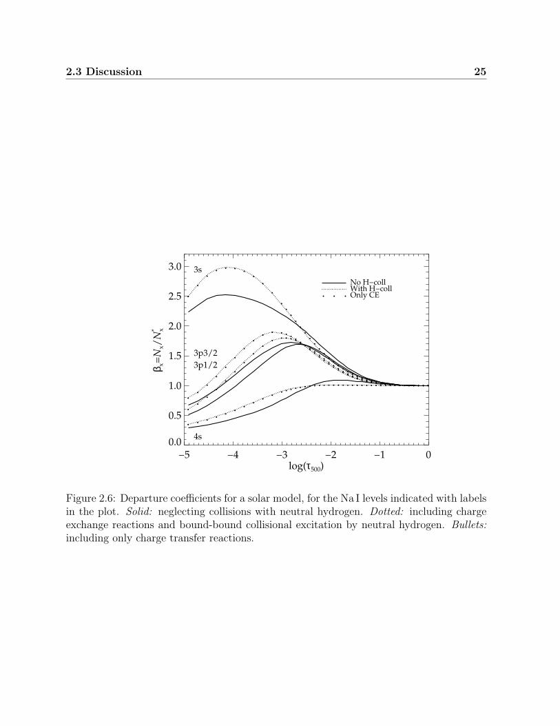
The quantum mechanical calculations by Barklem et al. (2010) result in rate coefficientsfor collisional excitation by hydrogen atoms that are lower than the commonly used classicalDrawin recipe, by one to six orders of magnitude. The new rates thus have very smallinfluence on the statistical equilibrium of Na I, in the stellar parameter range that weconsider here. However, again analogously to Li, charge exchange reactions turn out tobe much more influential. Fig. 2.6 illustrates how the departure coefficients of low excitedlevels change for a solar model, when including and neglecting collisions with neutralhydrogen.
It is conceptually correct to say that higher collisional rates have a thermalising effect,i.e. tend to drive the level population towards LTE. However, as seen for the Sun inFig. 2.6, this is not generally true for all levels. The populations of the ground state andfirst excited states are rather pushed further from LTE in shallow atmospheric layers, whencharge exchange is included. This seemingly contradictory behaviour can be understoodby realising that the collisional cross-sections of 3s and 3p are very small, and the changesin their level population are rather a secondary effect, stemming from the thermalisationof higher excited levels. Especially, 4s, whose departure coefficients are also displayedin Fig. 2.6, has a large cross-section for charge exchange and the level becomes almostthermalised with the inclusion of this process. In deep layers, where β4s > 1, the over-recombination of Na I is lessened, decreasing the over-population of the level itself, but alsolower excited levels. In shallow layers, where β4s < 1, recombination is enhanced, lesseningthe under-population of 4s, but increasing further the over-population of lower levels. Inpractise, also excited levels higher than 4s influence the outcome, but to a smaller extent.
Even if the statistical equilibrium is indeed influenced by hydrogen collisions, thestrengths of the emergent spectral lines need not necessarily be so. This is due to thefact that the source functions remain unchanged, and as discussed above, the effect onthe level populations of 3s and 3p is opposite in different regimes of the atmosphere, sothat the net effect on the line strength is small. The situation is a bit different from that
24 2. Non-LTE calculations for neutral Na using improved atomic data
−0.55
−0.50
−0.45
−0.40
−0.35
−0.30
−0.25
−0.20
−0.15
−0.10
−0.05
Teff
log(g)
[Fe/H]=−3λ=589.5nm
Teff
[Fe/H]=−3λ=818.3nm
log(g)
[Fe/H]=−2λ=589.5nm
[Fe/H]=−2λ=818.3nm
log(g)
[Fe/H]=−1λ=568.2nm
[Fe/H]=−1λ=615.4nm
log(g)
[Fe/H]=+0λ=568.2nm
[Fe/H]=+0λ=615.4nm
Figure 2.5: Contour diagrams illustrating how the abundance corrections vary with effectivetemperature and surface gravity, for four lines commonly analysed lines of Na I. Only theresults for ξ = 2km/s and [Na/Fe] = 0 are shown.
2.3 Discussion 25
−5 −4 −3 −2 −1 0log(τ500)
0.0
0.5
1.0
1.5
2.0
2.5
3.0
β x=
Nx/
N* x
3s
3p3/2
3p1/2
4s
No H−collWith H−collOnly CE
Figure 2.6: Departure coefficients for a solar model, for the Na I levels indicated with labelsin the plot. Solid: neglecting collisions with neutral hydrogen. Dotted: including chargeexchange reactions and bound-bound collisional excitation by neutral hydrogen. Bullets:including only charge transfer reactions.
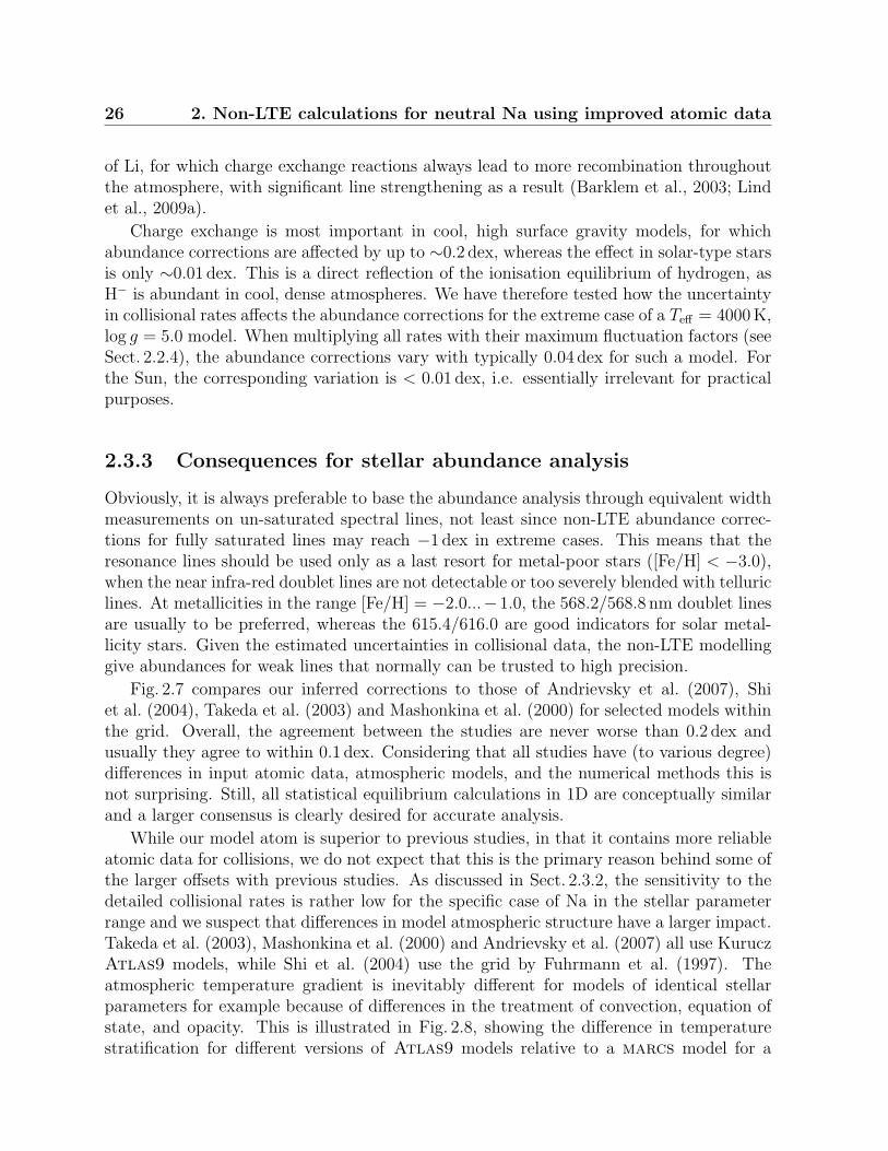
26 2. Non-LTE calculations for neutral Na using improved atomic data
of Li, for which charge exchange reactions always lead to more recombination throughoutthe atmosphere, with significant line strengthening as a result (Barklem et al., 2003; Lindet al., 2009a).
Charge exchange is most important in cool, high surface gravity models, for whichabundance corrections are affected by up to ∼0.2 dex, whereas the effect in solar-type starsis only ∼0.01 dex. This is a direct reflection of the ionisation equilibrium of hydrogen, asH− is abundant in cool, dense atmospheres. We have therefore tested how the uncertaintyin collisional rates affects the abundance corrections for the extreme case of a Teff = 4000K,log g = 5.0 model. When multiplying all rates with their maximum fluctuation factors (seeSect. 2.2.4), the abundance corrections vary with typically 0.04 dex for such a model. Forthe Sun, the corresponding variation is < 0.01 dex, i.e. essentially irrelevant for practicalpurposes.
2.3.3 Consequences for stellar abundance analysis
Obviously, it is always preferable to base the abundance analysis through equivalent widthmeasurements on un-saturated spectral lines, not least since non-LTE abundance correc-tions for fully saturated lines may reach −1 dex in extreme cases. This means that theresonance lines should be used only as a last resort for metal-poor stars ([Fe/H] < −3.0),when the near infra-red doublet lines are not detectable or too severely blended with telluriclines. At metallicities in the range [Fe/H] = −2.0...−1.0, the 568.2/568.8 nm doublet linesare usually to be preferred, whereas the 615.4/616.0 are good indicators for solar metal-licity stars. Given the estimated uncertainties in collisional data, the non-LTE modellinggive abundances for weak lines that normally can be trusted to high precision.
Fig. 2.7 compares our inferred corrections to those of Andrievsky et al. (2007), Shiet al. (2004), Takeda et al. (2003) and Mashonkina et al. (2000) for selected models withinthe grid. Overall, the agreement between the studies are never worse than 0.2 dex andusually they agree to within 0.1 dex. Considering that all studies have (to various degree)differences in input atomic data, atmospheric models, and the numerical methods this isnot surprising. Still, all statistical equilibrium calculations in 1D are conceptually similarand a larger consensus is clearly desired for accurate analysis.
While our model atom is superior to previous studies, in that it contains more reliableatomic data for collisions, we do not expect that this is the primary reason behind some ofthe larger offsets with previous studies. As discussed in Sect. 2.3.2, the sensitivity to thedetailed collisional rates is rather low for the specific case of Na in the stellar parameterrange and we suspect that differences in model atmospheric structure have a larger impact.Takeda et al. (2003), Mashonkina et al. (2000) and Andrievsky et al. (2007) all use KuruczAtlas9 models, while Shi et al. (2004) use the grid by Fuhrmann et al. (1997). Theatmospheric temperature gradient is inevitably different for models of identical stellarparameters for example because of differences in the treatment of convection, equation ofstate, and opacity. This is illustrated in Fig. 2.8, showing the difference in temperaturestratification for different versions of Atlas9 models relative to a marcs model for a
2.3 Discussion 27
4500 5000 5500 6000 6500Teff
−0.6
−0.5
−0.4
−0.3
−0.2
−0.1
−0.0
∆A(N
a)
Andrievsky et al (2007) [Fe/H]=−3.0
5889
5895
1.4 2.0 2.7 3.3 3.7 4.1
5400 5600 5800 6000 6200 6400 6600−1.0
−0.8
−0.6
−0.4
−0.2
0.0
∆A(N
a)
Takeda et al (2003) [Fe/H]=−2.0
5895
8194
4.0 4.0
4000 5000 6000 7000 8000
−0.5
−0.4
−0.3
−0.2
−0.1
0.0
∆A(N
a)
8183
5688
Mashonkina et al (2000) [Fe/H]=−1.0
1.0 1.5 2.0 2.5 3.0 3.5 4.0 4.5 4.5
5000 5500 6000 6500
−0.20
−0.15
−0.10
−0.05
0.00
∆A(N
a)
Shi et al (2004) [Fe/H]=+0.0
5682
6154
4.0 4.0 4.0 4.0log(g)
Figure 2.7: Comparison between the abundance corrections determined in this study (linesconnected with bullets) and earlier studies, as indicated in each panel (lines connectedwith plus signs). The literature studies shown are, from the top to the bottom; Shi et al.(2004); Mashonkina et al. (2000); Takeda et al. (2003); Andrievsky et al. (2007). Effectivetemperature is used as reference axis, with surface gravity values for each model indicatedalong the top axis of each panel. All calculations used the assumption of [Na/Fe] = 0.0.
28 2. Non-LTE calculations for neutral Na using improved atomic data
metal-poor giant6. As can be seen in this figure, the stratification is critically dependenton the inclusion of convective over-shooting in the 1993 grid by Kurucz. The most up-to-date versions of Atlas9 (Castelli & Kurucz, 2004) and marcs (Gustafsson et al., 2008)both neglect over-shoot, and the models shown have similar, but not identical, parametersfor the mixing length, but nevertheless show differences on the 100K level.
The lower panel of Fig. 2.8 illustrates the effect on derived non-LTE abundance correc-tions for the 819.4 nm line, when using different atmospheric models. At low line strength,the height of the plateau appears, as expected, to be connected to the temperature gradientaround log(τ500) = 0. The Atlas9 model without over-shoot has the steepest gradient,producing a larger Jν−Bν-excess in the ultra-violet which counteracts over-recombination.The Atlas9 model with over-shoot has the flattest gradient, and thus the most negativecorrections. Still, the differences between the models are not large, <∼ 0.05 dex, for un-saturated lines. As seen in the plot, saturated lines show a larger sensitivity, and it is easilyappreciated that different model atmospheres can produce results that are discrepant bymore than 0.1 dex for such a metal-poor giant. We also note that the largest discrepanciesbetween the non-LTE studies are indeed present for strong lines (the line strength increasesfrom right to left, with decreasing effective temperature in Fig. 2.7).
2.4 Conclusions
Using our calculated abundance corrections and/or non-LTE curves-of-growth for ten im-portant neutral Na I lines, Na abundances that are superior to those inferred with the LTEassumption can easily be obtained for late-type dwarf and giant stars. The results showa small sensitivity to uncertainties in input atomic data for collisional cross-sections, butare sensitive to the detailed structure of the atmosphere. To minimise the influence frompossible systematic errors in the model, un-saturated lines are definitely to be preferredas abundance indicators based on integrated line strengths. As always, a good test of thesoundness of the modelling procedure is to compare Na abundances from lines of differentstrengths.
In a forthcoming paper we will explore the impact of the model atmosphere on theabundance determination more closely, and extend our work to include 3D, hydrodynamicalmodel atmospheres, superseding the crude mixing length recipes used for convection instatic 1D models. The model atom presented here will then be applied to specific cases ofsolar-metallicity and metal-poor dwarfs and giants, and we will discuss the prospects foraccurate analysis of the Galactic chemical evolution of Na.
6The Atlas9 models were downloaded from http://kurucz.harvard.edu/grids/, with convectiveover-shoot (gridm20), without over-shoot (gridm20NOVER), and using more updated opacity and abun-dances (gridm20a2ODFNEW).
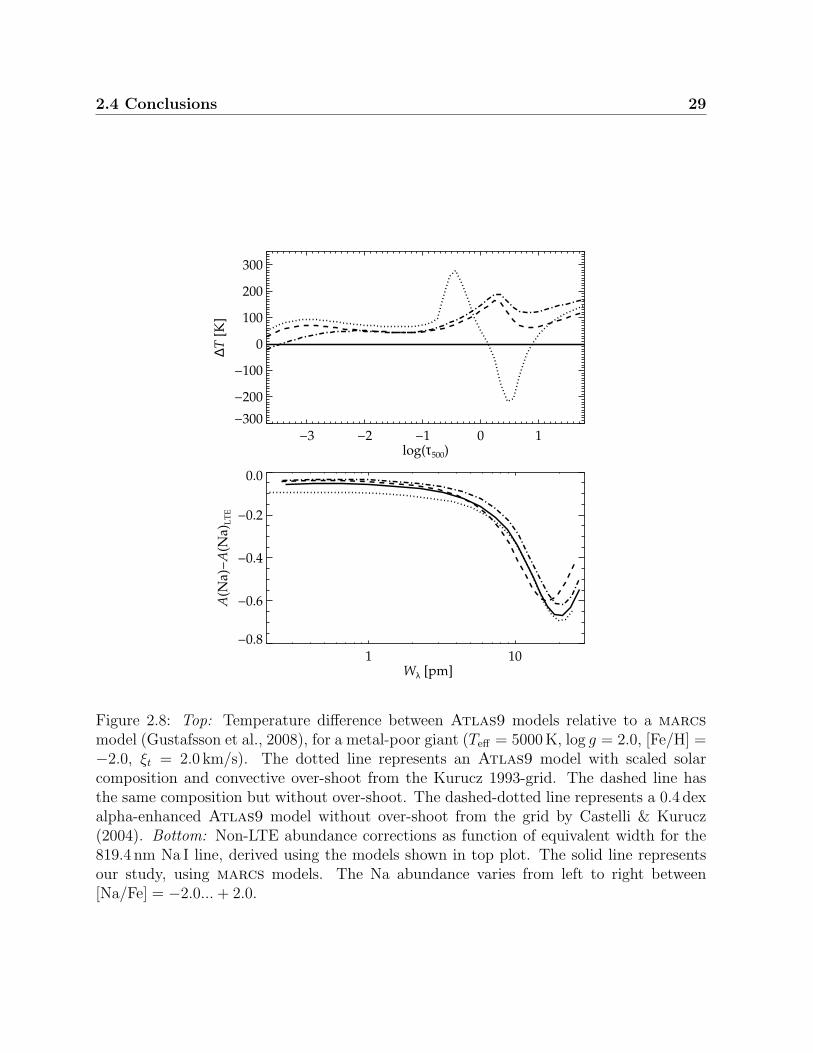
2.4 Conclusions 29
−3 −2 −1 0 1log(τ500)
−300
−200
−100
0
100
200
300
∆T [
K]
1 10Wλ [pm]
−0.8
−0.6
−0.4
−0.2
0.0
A(N
a)−A
(Na)
LT
E
Figure 2.8: Top: Temperature difference between Atlas9 models relative to a marcsmodel (Gustafsson et al., 2008), for a metal-poor giant (Teff = 5000K, log g = 2.0, [Fe/H] =−2.0, ξt = 2.0 km/s). The dotted line represents an Atlas9 model with scaled solarcomposition and convective over-shoot from the Kurucz 1993-grid. The dashed line hasthe same composition but without over-shoot. The dashed-dotted line represents a 0.4 dexalpha-enhanced Atlas9 model without over-shoot from the grid by Castelli & Kurucz(2004). Bottom: Non-LTE abundance corrections as function of equivalent width for the819.4 nm Na I line, derived using the models shown in top plot. The solid line representsour study, using marcs models. The Na abundance varies from left to right between[Na/Fe] = −2.0... + 2.0.
30 2. Non-LTE calculations for neutral Na using improved atomic data
Chapter 3
Departures from LTE for neutral Li
The following chapter contains a modified version of an article that was published in As-tronomy & Astrophysics in August 2009 (Lind, Asplund, & Barklem).
3.1 Astrophysical motivation
Stellar lithium abundances are continuing to attract strong interest among the astronomicalcommunity. In particular, many studies are devoted to constraining and finding explana-tions for the famous “Spite plateau” of warm metal-poor halo stars, first discovered by Spite& Spite (1982). For recent studies of lithium in halo field stars see e.g. Ryan et al. (2001),Charbonnel & Primas (2005), Asplund et al. (2006), Bonifacio et al. (2007a), and Hosfordet al. (2009). To put constraints on the primordial lithium abundance in the Universe, itis of fundamental importance to determine if and by how much the Li abundances increasewith increasing metallicity on the Spite plateau. The behaviour of Li abundance witheffective temperature is of equal importance, as it could lend support to the notion thatatomic diffusion is acting in metal-poor stellar atmospheres. Lithium depletion throughatomic diffusion has been suggested as a solution to the discrepancy between the Spiteplateau abundance and the predicted value of the primordial lithium abundance (Kornet al., 2007; Lind et al., 2009b). To accurately infer both the mean lithium abundancein the halo and the abundance behaviour with metallicity and effective temperature, it iscrucial to have a realistic description of the lithium line formation. Previous non-LTE anal-yses spanning a large stellar-parameter space (Carlsson et al., 1994; Pavlenko & Magazzu,1996; Takeda & Kawanomoto, 2005) have shown that departures from LTE are generallysmall but significant at the required accuracy.
3.2 Non-LTE modelling procedure
We use the radiative-transfer code MULTI, version 2.3 (Carlsson, 1986, 1992) to per-form non-LTE calculations. The model atom used includes the same 20 energy levels for
32 3. Departures from LTE for neutral Li
neutral lithium as described in Carlsson et al. (1994), plus the Li II ground state. Thehighest considered level in Li I has principle quantum number n = 9. We have used TOP-base data (Peach et al., 1988) for energy levels, oscillator strengths, and photo-ionisationcross-sections for levels with orbital quantum number l ≤ 3. For the remaining levels,hydrogenic values are used. For the resonance line at 670.7 nm, we adopt the oscillatorstrength f = 0.7468, as calculated by Yan et al. (1998), and consider six hyperfine compo-nents in 7Li (neglecting 6Li), with measured wavelengths given by Sansonetti et al. (1995).For the subordinate line at 610.3 nm, we adopt f = 0.6386, also determined by Yan et al.(1998), and account for the three fine-structure components with wavelengths determinedby Lindgard & Nielson (1977). For both lines, van-der-Waals-broadening parameters followAnstee & O’Mara (1995) and Barklem & O’Mara (1997). Stark broadening is unimpor-tant in the late-type atmospheres of interest here and is therefore neglected. Table 3.1lists wavelengths, oscillator strengths, and broadening data adopted for the 670.7 nm and610.3 nm lines.
Cross-sections for collisional excitation by electrons are taken from Park (1971) andcollisional ionisation by electrons from Seaton (1962) as given by Allen (1976). We add ratecoefficients for excitation and de-excitation from collisions with neutral hydrogen atomsaccording to Belyaev & Barklem (2003) and Barklem et al. (2003), as well as charge transferreactions with neutral hydrogen and the negative hydrogen ion according to Croft et al.(1999). The number abundance of the negative hydrogen ion is calculated by assumingLTE. Ionisation by hydrogen atom impact is not included. For low-lying states at lowcollision energies, it is expected to be negligible compared to charge transfer reactions andexcitation (Krstic & Schultz, 2009).
A grid of 1D, LTE, opacity-sampling, MARCS model atmospheres (Gustafsson et al.,2008) is used in the analysis. Non-LTE computations for lithium as a trace elementare performed in the plane-parallel approximation, for models with Teff = 4000...8000K,log g = 1.0...5.0, [Fe/H] = 0.0... − 3.0, for lithium abundances in the range A(Li) =−0.30... − 4.20. The highest effective temperature is 5500K for models with log g = 1.0,6500K for log g = 2.0, 7500K for log g = 3.0, and 8000K for log g ≥ 4.0. For models withlog g ≥ 3.0, we adopted a microturbulence parameter ξt = 1.0 km s−1 and ξt = 2.0 km s−1,and for models with log g ≤ 3.0, we adopted ξt = 2.0 km s−1 and ξt = 5.0 km s−1. In total,392 atmospheric models are included in the computations.
In the statistical equilibrium calculations, the background opacity include continuumand line opacity provided by the MARCS model atmospheres. MULTI thus calculatesa line-blanketed photo-ionising radiation field while solving for the statistical equilibriumof lithium. Based on the LTE and non-LTE equivalent widths obtained for the stellar-parameter grid, we subsequently define a non-LTE correction for each abundance point asthe difference between its LTE lithium abundance and the non-LTE abundance that corre-sponds to the same equivalent width. The limiting equivalent widths for which correctionsare given are set to 0.01 pm and 100 pm. The equivalent width is obtained by numericalintegration over the line profile, considering a spectral region that extends ±9 nm from theline centre. For lines weaker than 50 pm the numerical precision is better than 0.01 pmwhereas the equivalent widths of the strongest lines are determined to within 0.1 pm.
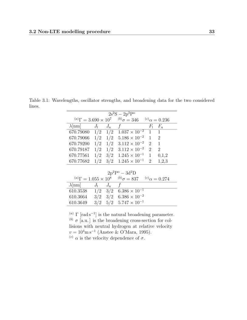
3.2 Non-LTE modelling procedure 33
Table 3.1: Wavelengths, oscillator strengths, and broadening data for the two consideredlines.
2s2S− 2p2Po
(a)Γ = 3.690× 10⁷ (b)σ = 346 (c)α = 0.236λ[nm] Jl Ju f Fl Fu
670.79080 1/2 1/2 1.037× 10⁻² 1 1670.79066 1/2 1/2 5.186× 10⁻² 1 2670.79200 1/2 1/2 3.112× 10⁻² 2 1670.79187 1/2 1/2 3.112× 10⁻² 2 2670.77561 1/2 3/2 1.245× 10⁻¹ 1 0,1,2670.77682 1/2 3/2 1.245× 10⁻¹ 2 1,2,3
2p2Po − 3d2D(a)Γ = 1.055× 10⁸ (b)σ = 837 (c)α = 0.274
λ[nm] Jl Ju f610.3538 1/2 3/2 6.386× 10⁻¹
610.3664 3/2 3/2 6.386× 10⁻²
610.3649 3/2 5/2 5.747× 10⁻¹
(a) Γ [rad s−1] is the natural broadening parameter.(b) σ [a.u. ] is the broadening cross-section for col-lisions with neutral hydrogen at relative velocityv = 104m s−1 (Anstee & O’Mara, 1995).(c) α is the velocity dependence of σ.
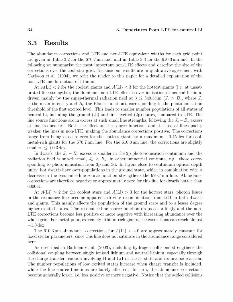
34 3. Departures from LTE for neutral Li
3.3 Results
The abundance corrections and LTE and non-LTE equivalent widths for each grid pointare given in Table 3.2 for the 670.7 nm line, and in Table 3.3 for the 610.3 nm line. In thefollowing we summarise the most important non-LTE effects and describe the size of thecorrections over the cool-star grid. Because our results are in qualitative agreement withCarlsson et al. (1994), we refer the reader to this paper for a detailed explanation of thenon-LTE line formation of lithium.
At A(Li) < 2 for the coolest giants and A(Li) < 3 for the hottest giants (i.e. at unsat-urated line strengths), the dominant non-LTE effect is over-ionisation of neutral lithium,driven mainly by the super-thermal radiation field at λ <∼ 349.5 nm (Jν > Bν , where Jν
is the mean intensity and Bν the Planck function), corresponding to the photo-ionisationthreshold of the first excited level. This leads to smaller number populations of all states ofneutral Li, including the ground (2s) and first excited (2p) states, compared to LTE. Theline source functions are in excess at such small line strengths, following the Jν−Bν excessat line frequencies. Both the effect on the source functions and the loss of line-opacityweaken the lines in non-LTE, making the abundance corrections positive. The correctionsrange from being close to zero for the hottest giants to a maximum +0.45 dex for cool,metal-rich giants for the 670.7 nm line. For the 610.3 nm line, the corrections are slightlysmaller, ≤ +0.3 dex.
In dwarfs, the Jν − Bν excess is smaller in the 2p photo-ionisation continuum and theradiation field is sub-thermal, Jν < Bν , in other influential continua, e.g. those corre-sponding to photo-ionisation from 3p and 3d. In layers close to continuum optical depthunity, hot dwarfs have over-populations in the ground state, which in combination with adecrease in the resonance-line source function strengthens the 670.7 nm line. Abundancecorrections are therefore negative or approximately zero for this line for dwarfs hotter than6000 K.
At A(Li) > 2 for the coolest stars and A(Li) > 3 for the hottest stars, photon lossesin the resonance line become apparent, driving recombination from Li II in both dwarfsand giants. This mainly affects the population of the ground state and to a lesser degreehigher excited states. The resonance-line source function drops accordingly and the non-LTE corrections become less positive or more negative with increasing abundance over thewhole grid. For metal-poor, extremely lithium-rich giants, the corrections can reach almost−1.0 dex.
The 610.3 nm abundance corrections for A(Li) < 4.0 are approximately constant forfixed stellar parameters, since this line does not saturate in the abundance range consideredhere.
As described in Barklem et al. (2003), including hydrogen collisions strengthens thecollisional coupling between singly ionised lithium and neutral lithium, especially throughthe charge transfer reaction involving H and Li I in the 3s state and its inverse reaction.The number populations of low excited states increase when charge transfer is included,while the line source functions are barely affected. In turn, the abundance correctionsbecome generally lower, i.e. less positive or more negative. Notice that the added collisions
3.4 Discussion 35
Table 3.2: Non-LTE abundance corrections and equivalent widths for the Li I λ = 670.7 nmline. The whole table can be retrieved in machine-readable format from the CDS: http://vizier.u-strasbg.fr/viz-bin/VizieR?-source=J/A+A/503/541.
Teff log g [Fe/H] ξt A(Li)LTE ∆(a) Wλ,LTE Wλ,NLTE
[K] [km/s] [pm] [pm]4000 1.0 -3.0 2.0 -0.3 0.25 2.24 1.294000 1.0 -3.0 2.0 0.0 0.25 4.20 2.494000 1.0 -3.0 2.0 0.3 0.25 7.48 4.654000 1.0 -3.0 2.0 0.6 0.24 12.28 8.284000 1.0 -3.0 2.0 0.9 0.21 18.05 13.664000 1.0 -3.0 2.0 1.2 0.14 23.71 20.40... ... ... ... ... ... ... ...(a) ∆ = A(Li)non−LTE − A(Li)LTE
do not always have a thermalising effect, but can contribute to over-population of levelscompared to LTE. The effect is illustrated in Fig.3.1, for a selected metal-poor and solar-metallicity dwarf and giant. As seen in Fig. 3.1, the change in A(Li)non−LTE − A(Li)LTE
when including charge transfer is −0.12 dex for the metal-poor giant and −0.06 dex for themetal-poor dwarf.
While the charge transfer reaction has a significant influence on the statistical equi-librium of lithium, including bound-bound (and bound-free) transitions due to collisionswith neutral hydrogen has no influence at all. However, this is not true if one relies on theclassical Drawin recipe for estimates of the cross-section for those collisions. For compari-son, Fig. 3.1 also shows the results obtained when neglecting charge transfer reactions butincluding excitation and ionisation by neutral hydrogen according to Drawin’s recipe, withthe rate formula given by Lambert (1993) and with the scaling factor SH = 1.0. Generally,the Drawin cross-sections are much higher than the quantum mechanical calculations byBelyaev & Barklem (2003). When adopting the higher classical rates, the ground state ismore populated and the abundance corrections become lower, by ∼ −0.05 dex, comparedto the results obtained with quantum mechanical rates.
3.4 Discussion
We have compared our results for the lithium resonance line to Carlsson et al. (1994) abun-dance corrections for dwarfs and giants with [Fe/H] = −3.0...0.0 to Pavlenko & Magazzu(1996) results for dwarfs and subgiants with solar metallicity and to Takeda & Kawanomoto(2005) corrections for dwarfs and subgiants with [Fe/H] = −1.0...0.0 (see Fig. 3.3). To aidin the comparison we converted the LTE and non-LTE equivalent widths listed in Table 1in Pavlenko & Magazzu (1996) to abundance corrections. The largest difference is 0.12 dexbetween our results and those of Pavlenko & Magazzu (1996) and 0.15 dex between our
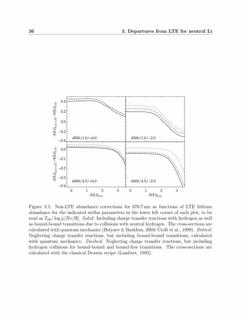
36 3. Departures from LTE for neutral Li
−0.4
−0.2
0.0
0.2
0.4
A(L
i)n
on
−L
TE−
A(L
i)L
TE
4500/1.0/+0.0
4500/1.0/−2.0
0 1 2 3A(Li)LTE
−0.4
−0.3
−0.2
−0.1
0.0
A(L
i)n
on
−L
TE−
A(L
i)L
TE
6000/4.5/+0.0
0 1 2 3A(Li)LTE
6000/4.5/−2.0
Figure 3.1: Non-LTE abundance corrections for 670.7 nm as functions of LTE lithiumabundance for the indicated stellar parameters in the lower left corner of each plot, to beread as Teff/ log g/[Fe/H]. Solid: Including charge transfer reactions with hydrogen as wellas bound-bound transitions due to collisions with neutral hydrogen. The cross-sections arecalculated with quantum mechanics (Belyaev & Barklem, 2003; Croft et al., 1999). Dotted:Neglecting charge transfer reactions, but including bound-bound transitions, calculatedwith quantum mechanics. Dashed: Neglecting charge transfer reactions, but includinghydrogen collisions for bound-bound and bound-free transitions. The cross-sections arecalculated with the classical Drawin recipe (Lambert, 1993).
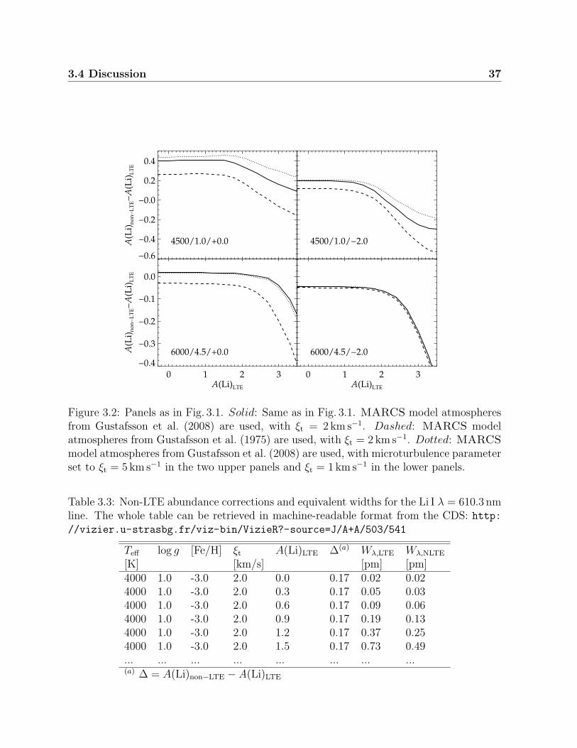
3.4 Discussion 37
−0.6
−0.4
−0.2
−0.0
0.2
0.4
A(L
i)n
on
−L
TE−
A(L
i)L
TE
4500/1.0/+0.0
4500/1.0/−2.0
0 1 2 3A(Li)LTE
−0.4
−0.3
−0.2
−0.1
0.0
A(L
i)n
on
−L
TE−
A(L
i)L
TE
6000/4.5/+0.0
0 1 2 3A(Li)LTE
6000/4.5/−2.0
Figure 3.2: Panels as in Fig. 3.1. Solid: Same as in Fig. 3.1. MARCS model atmospheresfrom Gustafsson et al. (2008) are used, with ξt = 2 km s−1. Dashed: MARCS modelatmospheres from Gustafsson et al. (1975) are used, with ξt = 2 km s−1. Dotted: MARCSmodel atmospheres from Gustafsson et al. (2008) are used, with microturbulence parameterset to ξt = 5 km s−1 in the two upper panels and ξt = 1 km s−1 in the lower panels.
Table 3.3: Non-LTE abundance corrections and equivalent widths for the Li I λ = 610.3 nmline. The whole table can be retrieved in machine-readable format from the CDS: http://vizier.u-strasbg.fr/viz-bin/VizieR?-source=J/A+A/503/541
Teff log g [Fe/H] ξt A(Li)LTE ∆(a) Wλ,LTE Wλ,NLTE
[K] [km/s] [pm] [pm]4000 1.0 -3.0 2.0 0.0 0.17 0.02 0.024000 1.0 -3.0 2.0 0.3 0.17 0.05 0.034000 1.0 -3.0 2.0 0.6 0.17 0.09 0.064000 1.0 -3.0 2.0 0.9 0.17 0.19 0.134000 1.0 -3.0 2.0 1.2 0.17 0.37 0.254000 1.0 -3.0 2.0 1.5 0.17 0.73 0.49... ... ... ... ... ... ... ...(a) ∆ = A(Li)non−LTE − A(Li)LTE
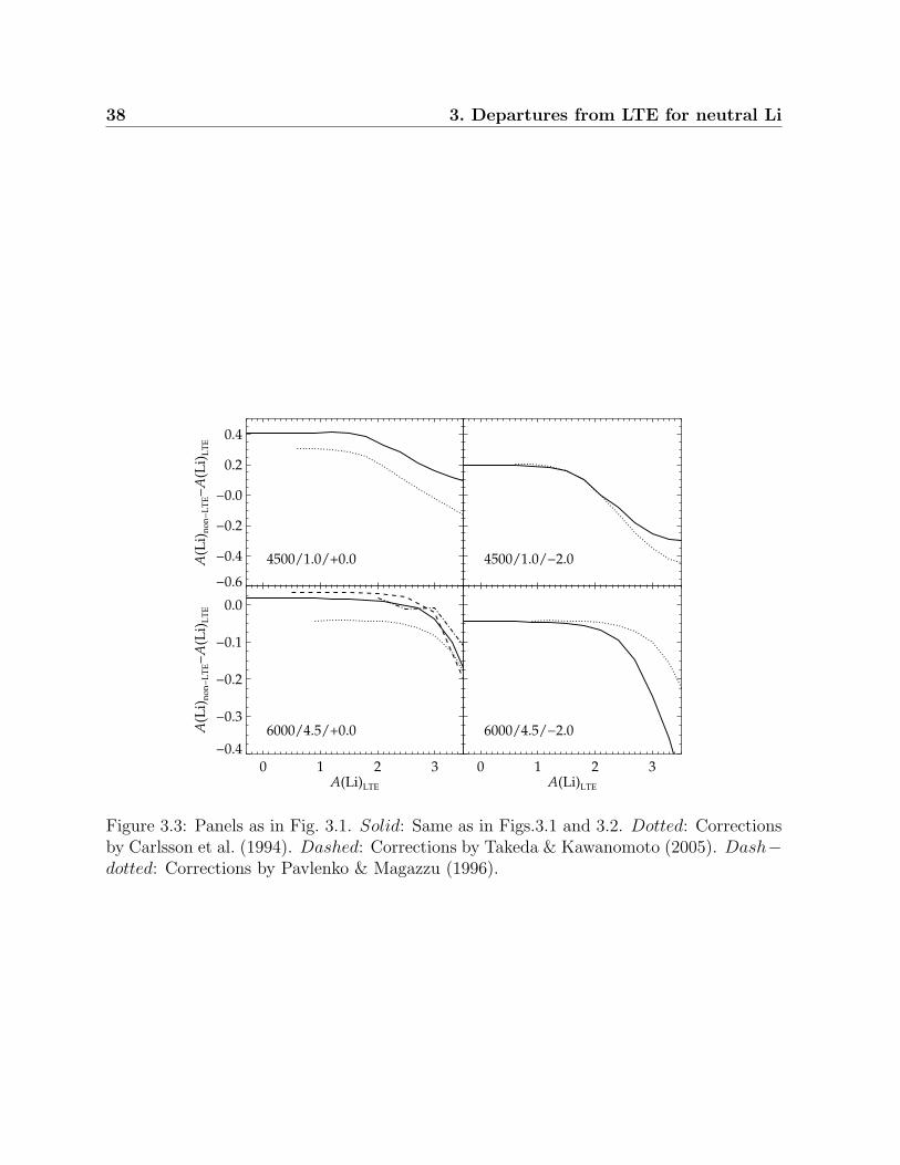
38 3. Departures from LTE for neutral Li
−0.6
−0.4
−0.2
−0.0
0.2
0.4
A(L
i)n
on
−L
TE−
A(L
i)L
TE
4500/1.0/+0.0
4500/1.0/−2.0
0 1 2 3A(Li)LTE
−0.4
−0.3
−0.2
−0.1
0.0
A(L
i)n
on
−L
TE−
A(L
i)L
TE
6000/4.5/+0.0
0 1 2 3A(Li)LTE
6000/4.5/−2.0
Figure 3.3: Panels as in Fig. 3.1. Solid: Same as in Figs.3.1 and 3.2. Dotted: Correctionsby Carlsson et al. (1994). Dashed: Corrections by Takeda & Kawanomoto (2005). Dash−dotted: Corrections by Pavlenko & Magazzu (1996).
3.4 Discussion 39
results and those of Takeda & Kawanomoto (2005), but generally the values agree quitewell. The Carlsson et al. (1994) values agree with ours to within 0.15 dex for dwarfs and0.20 dex for giants. Such differences are reasonable considering differences in the modelatom and in the atmospheric models. Carlsson et al. (1994) use Gustafsson et al. (1975)MARCS models and Takeda & Kawanomoto (2005) and Pavlenko & Magazzu (1996) useKurucz (1993) ATLAS9 models. The effects on the non-LTE abundance corrections whenusing MARCS models from Gustafsson et al. (1975) and Gustafsson et al. (2008) areillustrated in Fig. 3.2. Especially for the two giants, the choice of model atmosphere is im-portant for the corrections. The newer models include more line opacity, causing a steepertemperature gradient in the upper part of the photosphere, which increases the ultravioletJν − Bν excess and leads to more over-ionisation. The use of newer model atmospheresthus leads to more positive or less negative abundance corrections and partly cancels withthe effect of including hydrogen collisions (see Sect. 3.3)
Varying the microturbulence between 1 km s−1 and 2 km s−1 barely affects the abun-dance corrections (lower panels in Fig. 3.2), especially for low lithium abundances. In agiant star, the non-LTE abundance corrections become systematically higher when adopt-ing a microturbulence of 5 km s−1 instead of 2 km s−1, the differences being especially sig-nificant when the line is strong (upper panels Fig. 3.2). However, the parameter still hassome significance at low lithium abundances, when the formation of the line itself is un-affected by the microturbulence. This is because the choice of microturbulence influencesthe amount of line opacity included in the computations of the model atmosphere andconsequently also the atmospheric temperature gradient, which in turn partly drives thedepartures from LTE.
Our results are valid within the assumptions of 1D model atmospheres in LTE andhydrostatic equilibrium. Non-LTE calculations for lithium in 3D, hydrodynamical modelatmospheres have to this date been performed only for a few types of stars (Asplund et al.,2003), and we plan to extend our work to 3D in the future.
40 3. Departures from LTE for neutral Li
Chapter 4
3D, non-LTE line formation of Na Iin the Sun
In this chapter we explore departures from LTE for Na I in a realistic 3D hydrodynamicalmodel of the solar atmosphere. The results will be described in a forthcoming article inAstronomy & Astrophysics (Lind, Asplund, Barklem, Leenaarts, & Pereira). The intro-ductory section (Sect. 4.1) has been adopted from Asplund & Lind (2010).
4.1 Introduction
Traditionally, abundance analyses of late-type stars have been carried out relying on 1D,time-independent, hydrostatic model atmospheres, which treat convection with the rudi-mentary mixing length theory. All of these are dubious approximations as even a casualglance at the solar atmosphere will immediately reveal. The solar atmosphere, as for otherlate-type stars, is dominated by granulation, which is the observational manifestation ofconvection: an evolving pattern of broad, warm up-flows in the midst of narrow cooldowndrafts. Because of the great temperature sensitivity of the opacity, the temperaturedrops precipitously as the ascending gas nears the optical surface before it overturns andis accelerated downwards. The temperature contrast is therefore very pronounced in thephotospheric layers, amounting to > 1000K at the optical surface for the Sun (even whenaveraged over surfaces of equal optical depths these rms-differences amount to 400K). Inaddition to ignoring such atmospheric inhomogeneities, 1D model atmospheres can notbe expected to have the correct mean temperature stratification because of the simplifiedconvection treatment and the neglect of convective overshoot. Even small temperaturedifferences can propagate to very large changes in the emergent stellar spectrum becauseof the non-linearities in the radiative transfer and the extreme opacity variations.
Over the past decade or so, 3D, time-dependent, hydrodynamical model atmospheresfor a range of stellar parameters have started to be developed and applied to stellar abun-dance work (e.g. Asplund 2005, and references therein). Such 3D models solve the stan-dard hydrodynamical conservation equations coupled with a simultaneous solution of the
42 4. 3D, non-LTE line formation of Na I in the Sun
3D radiative transfer equation and therefore self-consistently predict the convective andradiative energy transport (see e.g. Nordlund et al. 2009, for further details). To make the3D modelling computationally tractable, the radiative transfer is not solved for the manythousands of wavelength points as routinely done in 1D model atmosphere codes. Insteadthe frequencies are sorted in opacity and more recently also in wavelength space for 4− 20bins for which the radiative transfer is solved. The resulting total radiative heating/coolingas a function of atmospheric depth is surprisingly well reproduced. The 3D models arebased on similarly realistic microphysics (equation-of-state and continuous/line opacity)as employed in standard 1D model atmospheres. Currently there are mainly four differentcodes being used to develop 3D models; stagger (e.g. Nordlund et al. 2009), co5bold(e.g. Ludwig et al. 2009), muram (e.g. Vogler et al. 2005) and antares (e.g. Muthsamet al. 2010), although essentially all abundance related work to date has been performedwithin the first two collaborations.
Being more sophisticated in the modelling does not automatically translate to beingmore realistic. Over the past few years, substantial effort has therefore been dedicatedto verify the suitability of the 3D models for quantitative stellar spectroscopy using anarsenal of observational diagnostics. Some of the striking successes are that the 3D modelsaccurately predict the detailed solar granulation properties (e.g. Nordlund et al. 2009)as well as spectral line profiles, including their asymmetries and shifts (e.g. Asplundet al. 2000), which strongly suggests that the 3D modelling captures the essence of the realatmospheric structure and macroscopic gas motions. Another crucial test is the continuumcentre-to-limb variation, which is an excellent probe of the mean temperature stratificationin the solar atmosphere. The latest generation of 3D models computed with the staggercode reproduces the observations extremely well (Pereira et al., submitted); the co5boldsolar model does a similarly good job (H.-G. Ludwig, private communication). This is aremarkable achievement. The 3D solar model not only outperforms all tested theoretical1D model atmospheres like the atlas, marcs and phoenix flavours in this respect, italso does noticeably better than the semi-empirical model by Holweger & Mueller (1974),which was constructed largely to fulfil this observational constraint. The 3D solar modelalso performs very well when confronted with other tests, such as the spectral energydistribution, H lines (Pereira et al., submitted) and spatially resolved line profiles (Pereiraet al., 2009b,a). In all aspects the most recent 3D solar models are clearly highly realisticand can therefore safely be trusted for abundance analysis purposes (Asplund et al., 2009).
4.2 Modelling procedure
To compute Na lines in LTE and non-LTE in 3D, we solve for the radiative transferon multiple snapshots from a realistic 3D, time-dependent, hydro-dynamical simulation.The 3D model atmosphere was computed with an updated version of the stagger code,using 12 opacity bins (see Asplund et al. 2009). The 3D, LTE lines profiles have beencalculated by performing detailed radiative transfer on 90 snapshots, with 400 × 400 ×250 grid-points. The selected time series has a total flux corresponding to < Teff >=
4.2 Modelling procedure 43
5777 ± 10K. Each snapshot corresponds to a Cartesian box of 6 × 6 × 1Mm, with ahorizontal extension that spans over a handful of granules (see Fig. 4.4). To improvethe accuracy of the line formation calculations, the original simulation (extending downto 3Mm below the optical surface) has been interpolated to a finer vertical resolution.These calculations were performed with the newly developed code scate (Hayek et al.,submitted), which is an MPI code for 3D, LTE line formation with continuum scatteringtreated properly. The line profile is then spatially and temporally averaged, using all 90snapshots. Fig. 4.1 illustrates the temperature and electron density stratifications of onesuch 3D model snapshot compared to a standard 1D model (Gustafsson et al., 2008).
With the added complexity of non-LTE, even if limited to a single species, computerpower becomes essential to meet the precision demand of abundance work. To thus savecomputing time, we calculated the detailed non-LTE line profiles for only three represen-tative snapshots (∼ 100× 100× 80) using the code multi3d. For the same snapshots, wealso computed the LTE profiles with the same code and multiplied the averaged non-LTEto LTE ratio with the 3D, LTE profiles from the more rigorous calculations with scate.This profile ratio is fairly invariant from snapshot to snapshot, and can thus be reliablyestablished with this technique. multi3d is a domain-decomposed and MPI-parallellisedcode for statistical equilibrium and radiative transfer calculations in 3D, based on the orig-inal codes by (Botnen, 1997; Carlsson et al., 1994), with extensive further development(see e.g. Leenaarts & Carlsson 2009 for more details).
multi3d uses a short-characteristic radiative transfer scheme to compute the radi-ation field that is needed to establish the statistical equilibrium. The essence of thistechnique lies in that it solves the radiative transfer equation through multiple short rays,crossing through each grid point and extending to the cell face boundaries. We use theA4-quadrature by Carlson (1963), i.e. 24 rays in total intersect each point. To obtain thevalues of the source function at the boundaries, second-order Bezier interpolation is used.Once the iterative procedure has converged to a solution for the level populations of eachgrid point (∆Nx/Nx < 10−3), a long-characteristic Feautrier solver is used to predict theemergent intensity for different viewing angles.
The 1D results shown here for comparison have been obtained as described in Chapter2, using a marcs model atmosphere (Gustafsson et al., 2008) or the semi-empirical modelby Holweger & Mueller (1974, H-M model). The non-LTE calculations uses the codeMULTI2.3. multi3d and MULTI2.3 can be supplied with identical atomic data andbackground opacity and they give consistent results for 1D models.
The atomic model is the same as was described in detail in Chapter 2, with some minormodifications. Here, we include 20 levels of Na I, coupled via 122 bound-bound radiativetransition and 186 collisional transitions. All levels are radiationally and collisionally cou-pled to the ground state of Na II. Except for the separate treatment of the fine structurelevels of Na I 3p, we neglect line asymmetry due to fine- and hyperfine structure.
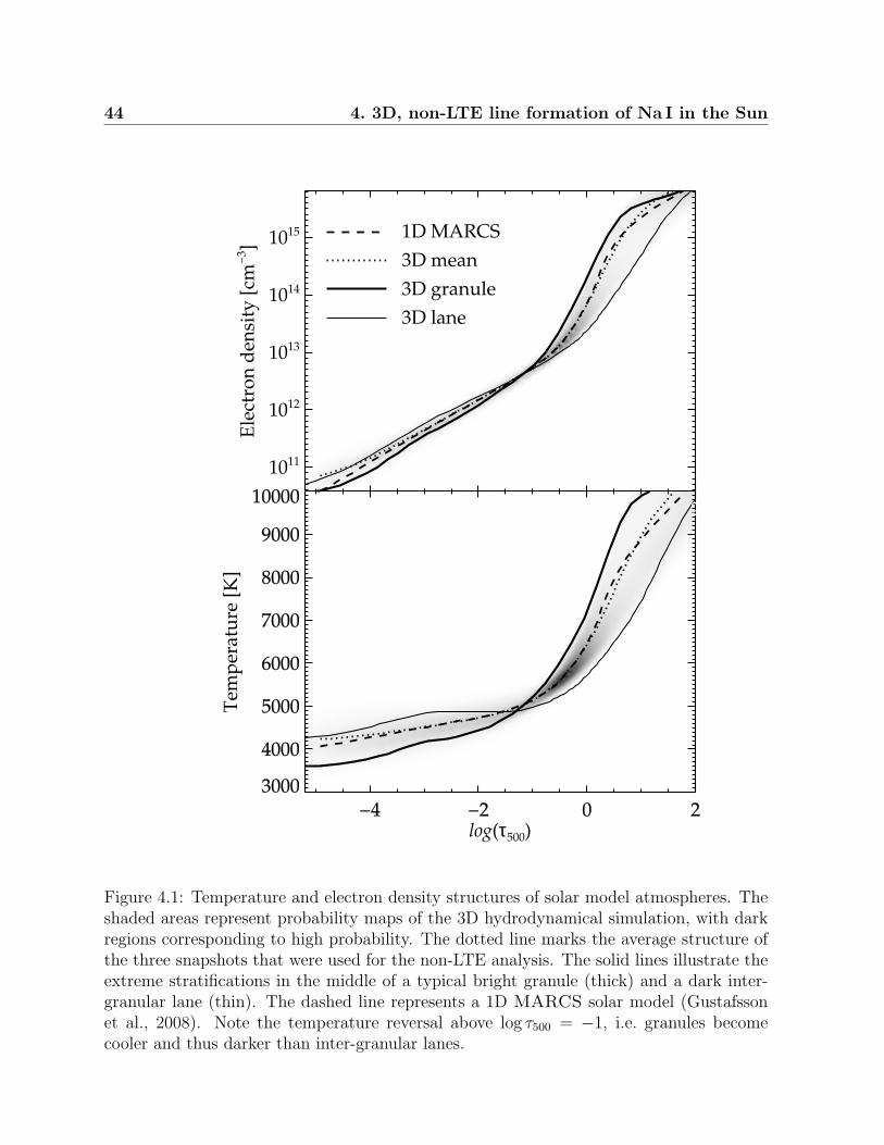
44 4. 3D, non-LTE line formation of Na I in the Sun
−4 −2 0 2log(τ500)
3000
4000
5000
6000
7000
8000
9000
10000
Tem
per
atu
re [
K]
−4 −2 0 23000
4000
5000
6000
7000
8000
9000
10000
−4 −2 0 23000
4000
5000
6000
7000
8000
9000
10000
1011
1012
1013
1014
1015
Ele
ctro
n d
ensi
ty [
cm−
3 ]
−4 −2 0 2
1D MARCS
3D mean
3D granule
3D lane
Figure 4.1: Temperature and electron density structures of solar model atmospheres. Theshaded areas represent probability maps of the 3D hydrodynamical simulation, with darkregions corresponding to high probability. The dotted line marks the average structure ofthe three snapshots that were used for the non-LTE analysis. The solid lines illustrate theextreme stratifications in the middle of a typical bright granule (thick) and a dark inter-granular lane (thin). The dashed line represents a 1D MARCS solar model (Gustafssonet al., 2008). Note the temperature reversal above log τ500 = −1, i.e. granules becomecooler and thus darker than inter-granular lanes.
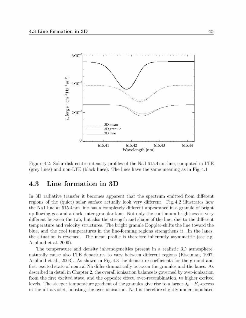
4.3 Line formation in 3D 45
615.41 615.42 615.43 615.44Wavelength [nm]
0
2•10−5
4•10−5
6•10−5
I ν [
erg
s−
1 cm
−2 H
z−1 s
r−1 ]
3D mean
3D granule
3D lane
Figure 4.2: Solar disk centre intensity profiles of the Na I 615.4 nm line, computed in LTE(grey lines) and non-LTE (black lines). The lines have the same meaning as in Fig. 4.1
4.3 Line formation in 3D
In 3D radiative transfer it becomes apparent that the spectrum emitted from differentregions of the (quiet) solar surface actually look very different. Fig. 4.2 illustrates howthe Na I line at 615.4 nm line has a completely different appearance in a granule of brightup-flowing gas and a dark, inter-granular lane. Not only the continuum brightness is verydifferent between the two, but also the strength and shape of the line, due to the differenttemperature and velocity structures. The bright granule Doppler-shifts the line toward theblue, and the cool temperatures in the line-forming regions strengthens it. In the lanes,the situation is reversed. The mean profile is therefore inherently asymmetric (see e.g.Asplund et al. 2000).
The temperature and density inhomogeneities present in a realistic 3D atmosphere,naturally cause also LTE departures to vary between different regions (Kiselman, 1997;Asplund et al., 2003). As shown in Fig. 4.3 the departure coefficients for the ground andfirst excited state of neutral Na differ dramatically between the granules and the lanes. Asdescribed in detail in Chapter 2, the overall ionisation balance is governed by over-ionisationfrom the first excited state, and the opposite effect, over-recombination, to higher excitedlevels. The steeper temperature gradient of the granules give rise to a larger Jν−Bν-excessin the ultra-violet, boosting the over-ionisation. Na I is therefore slightly under-populated
46 4. 3D, non-LTE line formation of Na I in the Sun
in the brightest regions, whereas the dark lanes rather show pronounced over-populationand lines that are stronger compared to LTE. Fig 4.4 illustrates clearly how both the LTEline strength and departures from LTE of the Na I 615.4 nm line correlates well with thepattern shaped by the convective motions.
4.4 Centre-to-limb variation
The close proximity of the Sun makes it possible to study its spectrum in much greaterdetail than other stars. In particular, observations that separates the light from differentregions of the stellar surface can provide invaluable information about the atmosphericconditions. In accordance with the Eddington-Barbier approximation (for the case of alinearly varying source function, I+
ν = Sν(τν = µ), Rutten 2003), light emitted closer tothe limb of the solar disk, i.e. having µ < 1, probe shallower layers, i.e. greater heights.The centre-to-limb variation of the solar intensity spectrum can thus serve as an excellenttest of the modelling of the atmospheric structure and line formation.
We have compared our synthetic spectra against spatially resolved solar observations,collected with the TRIPPEL spectrograph on the Swedish 1-m solar telescope on La Palma(Scharmer et al., 2003). A detailed description of the observations and data processing ispresented in Pereira et al. (2009b). The observational data have extremely high quality,with a signal-to-noise ratio of ∼ 1500, for the spatially averaged spectra, and a resolutionλ/δλ = 200000. The wavelength range covers the Na I 615.4 nm and 616.1 nm doublet,commonly used for abundance analyses of solar-metallicity stars. The centre-to-limb vari-ation of the Na I line strength was studied by forming the spatial and temporal mean offive sets of viewing angles (µ ≈ 0.2, 0.4, 0.6, 0.8, 1.0). The 1D and 3D results are shown inFigs. 4.5, comparing integrated line strengths, and 4.6, comparing the line profiles directly.
In 1D, two fudge factors must be adopted to reproduce observed line profiles, namelymicroturbulence, accounting for the effect that turbulent small-scale gas motions widen thecore of spectral lines, and macroturbulence, accounting for the Doppler shifts and therebyadditional line broadening induced by the large scale convective motions of rising andsinking gas. For the Sun we adopt a microturbulence ξt = 1km/s, and a radial-tangentialmacroturbulence ζRT = 2km/s (Gray, 2005). The 3D spectrum synthesis incorporatesthe velocity field resulting from hydro-dynamical simulations, and therefore do not requirethese parameters. Both 1D and 3D synthetic spectra are convolved with the instrumentalprofile and rotationally broadened, adopting v sin i = 2km/s. The equivalent widths ofmodel and observations have been computed by direct integration over a wavelength regionextending ±0.012 nm from the line centre, to exclude nearby lines from other metals. Inall comparisons, the Na abundance is adjusted to match the line strength at disk centre.
As is apparent from Fig. 4.5, traditional 1D, LTE modelling fails miserably to describethe centre-to-limb variation of the Na doublet, underestimating the line strengths at µ = 0.2by as much as 30%. 3D, LTE modelling performs better in comparison, although stillunderestimating the equivalent width. Non-LTE modelling in 1D does a much better jobin reproducing the observed equivalent widths, which gives confidence to the ability of the
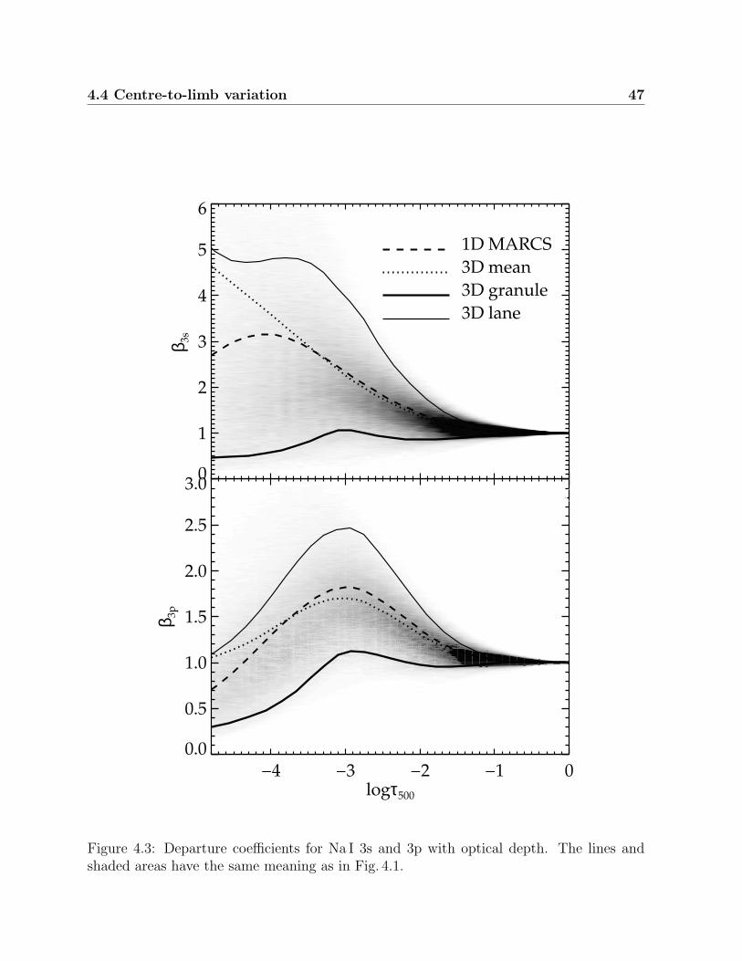
4.4 Centre-to-limb variation 47
−4 −3 −2 −1 0logτ500
0.0
0.5
1.0
1.5
2.0
2.5
3.0
β 3p
0
1
2
3
4
5
6
β 3s
−4 −3 −2 −1 0
1D MARCS
3D mean
3D granule
3D lane
Figure 4.3: Departure coefficients for Na I 3s and 3p with optical depth. The lines andshaded areas have the same meaning as in Fig. 4.1.
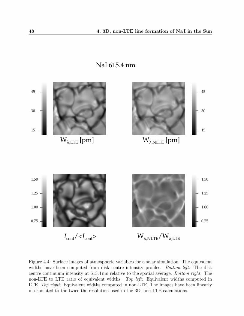
48 4. 3D, non-LTE line formation of Na I in the Sun
0.0 0.2 0.4 0.6 0.8 1.00.0
0.2
0.4
0.6
0.8
1.0
NaI 615.4 nm
Wλ,LTE [pm]
15
30
45
Wλ,NLTE [pm]
15
30
45
Icont/<Icont>
0.75
1.00
1.25
1.50
Wλ,NLTE/Wλ,LTE
0.75
1.00
1.25
1.50
Figure 4.4: Surface images of atmospheric variables for a solar simulation. The equivalentwidths have been computed from disk centre intensity profiles. Bottom left: The diskcentre continuum intensity at 615.4 nm relative to the spatial average. Bottom right: Thenon-LTE to LTE ratio of equivalent widths. Top left: Equivalent widths computed inLTE. Top right: Equivalent widths computed in non-LTE. The images have been linearlyinterpolated to the twice the resolution used in the 3D, non-LTE calculations.

4.4 Centre-to-limb variation 49
0.0 0.2 0.4 0.6 0.8 1.0µ
1D H−MNaI 615.4nm
0.0 0.2 0.4 0.6 0.8 1.0µ
3DNaI 615.4nm
0.0 0.2 0.4 0.6 0.8 1.0µ
2.0
2.5
3.0
3.5
4.0
4.5
5.0
Eq
uiv
alen
t w
idth
[p
m]
1D MARCSNaI 615.4nm
1D H−M
NaI 616.1nm
3D
NaI 616.1nm
3.5
4.0
4.5
5.0
5.5
6.0
6.5
Eq
uiv
alen
t w
idth
[p
m]
1D MARCS
NaI 616.1nm
Figure 4.5: Centre-to-limb variation of the equivalent widths of the Na I 615.4 nm and616.0 nm lines. The black bullets correspond to measurements of observed solar spectraand the lines represent different models. In each panel, the dashed line correspond toLTE and the solid line to non-LTE modelling including hydrogen collisions calculated byquantum mechanics. The left-hand and middle panels also shows the results obtained whenneglecting hydrogen collisions completely (dotted lines) and including hydrogen collisionscalculated with the classical Drawin recipe (dashed-dotted lines).

50 4. 3D, non-LTE line formation of Na I in the Sun
6153.8 6154.0 6154.2 6154.4 6154.6Wavelength [pm]
0.4
0.5
0.6
0.7
0.8
0.9
1.0
1.1
No
rmal
ised
in
ten
sity
1D
ξt=1km/s
ζRT=2km/s
A(Na)=6.25
6153.8 6154.0 6154.2 6154.4 6154.6Wavelength [pm]
3D
A(Na)=6.23
6160.4 6160.6 6160.8 6161.0 6161.2
0.4
0.6
0.8
1.0
No
rmal
ised
in
ten
sity
1D
ξt=1km/s
ζRT=2km/s
A(Na)=6.25
6160.4 6160.6 6160.8 6161.0 6161.2
3D
A(Na)=6.27
Figure 4.6: The solid lines represent the observed, normalised solar spectra at disk centre(µ = 1, top spectrum in each panel) and limb (µ = 0.2, normalised spectrum displaced by−0.2 for clarity). The dashed lines correspond to non-LTE modelling in 1D and 3D, as de-scribed in the text. The 1D synthetic spectrum has been computed with a MARCS model,adopting a microturbulence parameter of 1 km/s and a radial-tangential macroturbulenceof 2 km/s. The solar value of v sin i is assumed to be 2km/s.
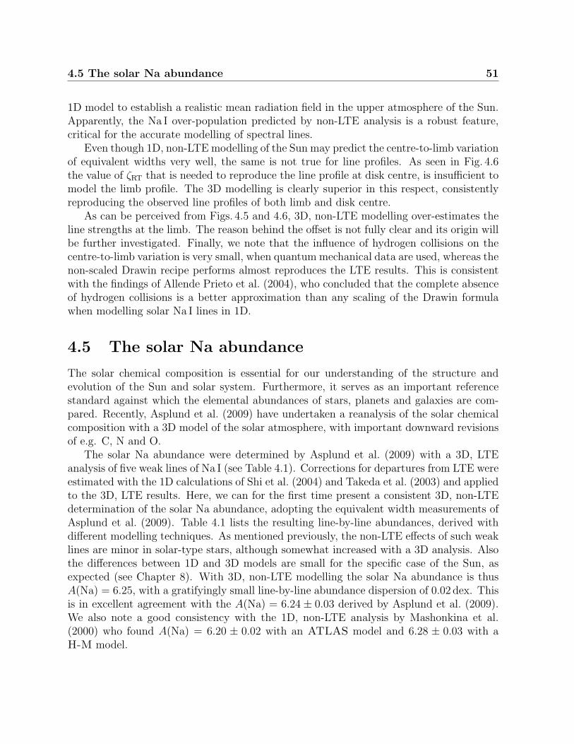
4.5 The solar Na abundance 51
1D model to establish a realistic mean radiation field in the upper atmosphere of the Sun.Apparently, the Na I over-population predicted by non-LTE analysis is a robust feature,critical for the accurate modelling of spectral lines.
Even though 1D, non-LTE modelling of the Sun may predict the centre-to-limb variationof equivalent widths very well, the same is not true for line profiles. As seen in Fig. 4.6the value of ζRT that is needed to reproduce the line profile at disk centre, is insufficient tomodel the limb profile. The 3D modelling is clearly superior in this respect, consistentlyreproducing the observed line profiles of both limb and disk centre.
As can be perceived from Figs. 4.5 and 4.6, 3D, non-LTE modelling over-estimates theline strengths at the limb. The reason behind the offset is not fully clear and its origin willbe further investigated. Finally, we note that the influence of hydrogen collisions on thecentre-to-limb variation is very small, when quantum mechanical data are used, whereas thenon-scaled Drawin recipe performs almost reproduces the LTE results. This is consistentwith the findings of Allende Prieto et al. (2004), who concluded that the complete absenceof hydrogen collisions is a better approximation than any scaling of the Drawin formulawhen modelling solar Na I lines in 1D.
4.5 The solar Na abundance
The solar chemical composition is essential for our understanding of the structure andevolution of the Sun and solar system. Furthermore, it serves as an important referencestandard against which the elemental abundances of stars, planets and galaxies are com-pared. Recently, Asplund et al. (2009) have undertaken a reanalysis of the solar chemicalcomposition with a 3D model of the solar atmosphere, with important downward revisionsof e.g. C, N and O.
The solar Na abundance were determined by Asplund et al. (2009) with a 3D, LTEanalysis of five weak lines of Na I (see Table 4.1). Corrections for departures from LTE wereestimated with the 1D calculations of Shi et al. (2004) and Takeda et al. (2003) and appliedto the 3D, LTE results. Here, we can for the first time present a consistent 3D, non-LTEdetermination of the solar Na abundance, adopting the equivalent width measurements ofAsplund et al. (2009). Table 4.1 lists the resulting line-by-line abundances, derived withdifferent modelling techniques. As mentioned previously, the non-LTE effects of such weaklines are minor in solar-type stars, although somewhat increased with a 3D analysis. Alsothe differences between 1D and 3D models are small for the specific case of the Sun, asexpected (see Chapter 8). With 3D, non-LTE modelling the solar Na abundance is thusA(Na) = 6.25, with a gratifyingly small line-by-line abundance dispersion of 0.02 dex. Thisis in excellent agreement with the A(Na) = 6.24 ± 0.03 derived by Asplund et al. (2009).We also note a good consistency with the 1D, non-LTE analysis by Mashonkina et al.(2000) who found A(Na) = 6.20 ± 0.02 with an ATLAS model and 6.28 ± 0.03 with aH-M model.
52 4. 3D, non-LTE line formation of Na I in the Sun
Table 4.1: The solar Na abundance as determined from disk centre equivalent width mea-surements of five Na I lines, taken from Asplund et al. (2009). The columns correspond todifferent atmospheric models, assuming Na I level populations in LTE and non-LTE.
λ [nm] Wλ [pm] A(Na)MARCS 1D H-M 1D 3D
LTE non-LTE LTE non-LTE LTE non-LTE
475.1822 1.11 6.25 6.24 6.32 6.28 6.26 6.23518.8838 1.27 6.22 6.20 6.30 6.26 6.27 6.24615.4225 3.73 6.25 6.21 6.33 6.27 6.31 6.27616.0747 5.70 6.22 6.17 6.31 6.23 6.33 6.281074.644 1.33 6.21 6.22 6.29 6.28 6.24 6.24< A(Na) > 6.23 6.21 6.31 6.26 6.28 6.25σ 0.02 0.03 0.02 0.02 0.04 0.02
Chapter 5
Globular clusters
The following chapter introduces the reader to the basic properties of globular star clustersand gives examples of what we may learn from chemical analysis of stars in these uniqueenvironments. Also, a short summary is given of multi-object, high-resolution spectroscopyand the necessary steps involved in observation, data processing, and abundance determi-nation.
5.1 Definition and basic properties
All stars in our Galaxy reside in either of its four main components; i.e. in the compactbulge in the centre, in the surrounding thin and thick disk holding the famous spiral arms,or in the extended spheroidal-shaped halo. Commonly, stars in the disk, with similarmetallicities to our Sun, are referred to as Pop I stars, whereas metal-poor halo stars arereferred to as Pop II. Halo stars are very rare compared to disk stars; the local numberdensity ratio between the halo and the thin disk is only ∼ 0.5 % (Juric et al., 2008).
The dense stellar conglomerates called globular clusters are found in the halo and thebulge, and all stars in the halo that do not belong to a globular cluster are simply called fieldstars. There is no one-parameter definition of a globular cluster, although it is generallyaccepted that they are very old (age >∼ 10 Gyr). The most complete catalogue (Harris,1996)1 contains 150 known clusters on elongated orbits of seemingly random orientationaround the Galactic centre. The majority of clusters are located within 20 kpc of the centre,but they can be found out to distances of 120 kpc (AM 1). Fig. 5.1 shows a schematic viewof the distribution of the known globular clusters in the Milky-Way.
Even among the Galactic globular clusters, there is large diversity in fundamentalproperties, such as mass, M = 103...107 M (Meylan & Heggie, 1997), metallicity, [Fe/H] =−2.4... + 0.07 (Gratton et al., 2004), and luminosity MV = −1.5...− 10.2 (Harris, 1996)2.
1with subsequent updates found at http://physwww.mcmaster.ca/∼harris/mwgc.dat2MV is the absolute visual magnitude. It is related to the bolometric magnitude, Mbol, via the bolo-
metric correction, BC, according to MV = Mbol − BC . The bolometric magnitude is defined from thestellar luminosity: Mbol −Mbol, = −2 .5 log(L/L)
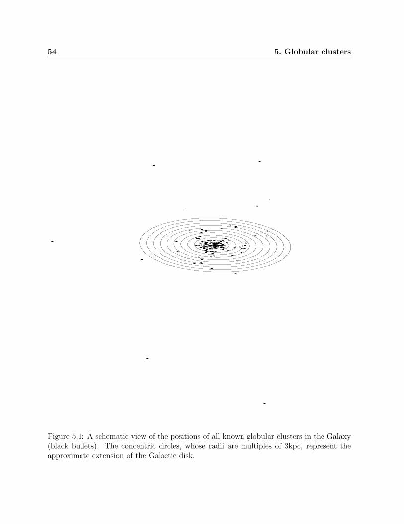
54 5. Globular clusters
−60−40
−200
2040
−60−40
−200
20
−50
0
50
100
Figure 5.1: A schematic view of the positions of all known globular clusters in the Galaxy(black bullets). The concentric circles, whose radii are multiples of 3kpc, represent theapproximate extension of the Galactic disk.
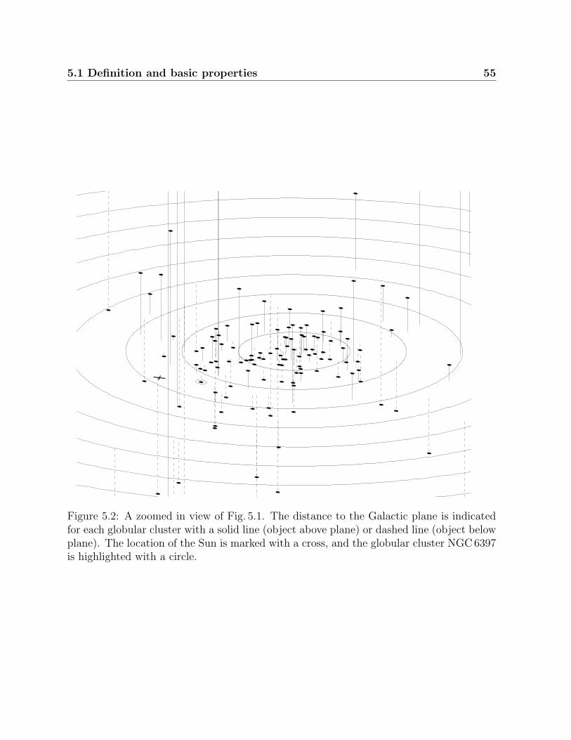
5.1 Definition and basic properties 55
−6−4
−20
24
6
−6−4
−20
24
6−6
−4
−2
0
2
4
6
Figure 5.2: A zoomed in view of Fig. 5.1. The distance to the Galactic plane is indicatedfor each globular cluster with a solid line (object above plane) or dashed line (object belowplane). The location of the Sun is marked with a cross, and the globular cluster NGC6397is highlighted with a circle.
56 5. Globular clusters
In fact, there is much evidence for the existence of two separate sub-populations of globularclusters, one metal-rich, more centrally concentrated and rapidly rotating, bulge systemand one metal-poor, more dispersed and slowly rotating, halo system (e.g. Brodie &Strader 2006). Our observational target in the following chapters is a nearby metal-poor(Pop II) globular cluster, NGC6397, which is part of the halo population. The location ofthis cluster is indicated with a circle in Fig. 5.2.
Concerning the distinction between globular clusters and open clusters, which generallycontain fewer stars and are much younger, one may base it on the presence or not of aO–Na anti-correlation (Carretta et al. 2010, see below), or on the different shapes of theluminosity functions of the two cluster types (van den Bergh, 1993). Dwarf spheroidalgalaxies, on the other hand, are generally bigger, more luminous and complex systems,and can be distinguished through their mass-to-light ratio, abundance spread in heavierelements or simply by shape (see e.g. discussion by van den Bergh 2008).
Globular clusters were long thought to be simple systems, both in terms of chemical anddynamical evolution. The idealistic view of a single stellar population of unique age andchemical composition, suffering only from slow evaporation due to dynamical relaxation,has been overturned by numerous observational evidence for multiple stellar populations(Sect. 6.1), the discovery of peculiar objects (blue stragglers, millisecond pulsars, ...), andthe realisation that a hypothetical central intermediate-mass black hole and processes likemass segregation, stellar mergers, and core collapse may affect the evolution. See Grat-ton et al. (2004) and Meylan & Heggie (1997) for extensive reviews of the chemical anddynamical properties of Galactic globular clusters.
5.2 Evolution of low-mass stars
To a first approximation, globular clusters are still considered to be rather simple, and theycan be extremely useful as laboratories for improving our knowledge of stellar physics andevolution. Under the hypothesis of uniform ages and chemical composition, the individualevolution of single stars in the cluster is almost uniquely determined by the stellar mass(neglecting e.g. rotational velocity). The HR-diagram of the cluster, i.e. a diagram withmagnitude (alias stellar luminosity) indicated on the y-axis and colour (alias effectivetemperature) on the x-axis, can then reveal the mass and evolutionary status of eachobject (see Figs. 5.3, 6.5, and 7.1).
Globular clusters are thought to be genuinely old, having experienced no further starformation since shortly after their formation in the very early universe. Therefore, theyhost (with few exceptions) only low-mass, long-lived stars. As an example, the expectedlife-time of a star like the Sun is roughly 10Gyr and more massive stars are thus extinct ina cluster of this age. The reader is referred to any textbook on the topic of stellar structureand evolution (e.g. Prialnik 2000) for a detailed description of the life and death of starsin different mass ranges.
Again, in the idealistic view of a globular cluster, the main sequence (MS) is a thin,tilted line in the HR-diagram, along which stars (alias dwarfs) of different masses are
5.3 Observational applications 57
distributed during the long-lasting quiescent H-burning phase. The MS ends on the high-mass, left-hand side, with the cluster turn-off (TO) point, which indicates the age of thecluster. Stars that are more massive have exhausted their fuel of hydrogen in the core, andstarted to move to the left in the HR diagram along the subgiant branch (SGB). In thisevolutionary phase, the envelope of the star cools and expands and the convective zoneextends inward, whilst hydrogen is burnt in a shell surrounding the contracting core. Theshell-burning continues as the star ascends the almost vertical red giant branch (RGB),and the core grows in size, while the convective envelope recedes. As will be discussedin Sect. 6.4.1, an important event in the stellar evolution occurs when hydrogen-burningshell crosses the boundary that marks the deepest penetration of the convective envelope,at the so called RGB bump. The red giant phase ends at the uppermost tip, when thestar ignites helium in its core (if it is massive enough). These giant phases of evolutionare very rapid compared to the MS life time and, as may be appreciated from Fig. 5.3, thevast majority of stars are thus MS stars, although the total light is dominated by the muchbrighter giants.
5.3 Observational applications
By spectroscopic analysis of stars, we can only infer the chemical composition of the veryoutermost layers, from which the light is emitted. Any chemical gradients or discontinuitiesin the stellar interior (i.e. below the outer convection zone, which is continuously mixedand thus chemically homogeneous) is beyond our reach to probe directly. Nevertheless, bycomparing stars of different masses and evolutionary phases, which presumably share thesame initial composition, we may trace such phenomena indirectly. Globular cluster starsare the obvious targets for such investigations. This methodology is discussed in detail inthe following chapter, where we analyse the post-MS evolution of the surface abundanceof lithium as well as the MS mass dependence (or, equivalently, the effective-temperaturedependence).
The main trigger of the observational project presented in Chapter 6 was the discrep-ancy between the Li abundances commonly observed in Pop II dwarfs and subgiant starsand the prediction of the primordial abundance, i.e. the small amounts of Li created inthe nucleosynthesis reactions that took place only minutes after the Big Bang. To alleviatethis factor of 2–5 discrepancy, it has been suggested that the stars observable today haveundergone photospheric depletion of lithium during their life times. The hypothesis is thatsome Li, and also other metals, has settled below the outer convection zone during thetime the star has spent on the MS. The photospheric composition of a MS star thereforedoes not correspond exactly to that it was born with. However, during the giant phases ofevolution the convective zone grows dramatically and erases any chemical differences in theaffected region, and we may once again see the initial elemental abundances at the surface.For Li, the situation is complicated by the fact that this light nuclei is destroyed in the hotstellar interiors and the surface abundance of giants therefore becomes severely diluted ata certain point in their evolution. By comparing Li abundances of dwarfs and giants, we
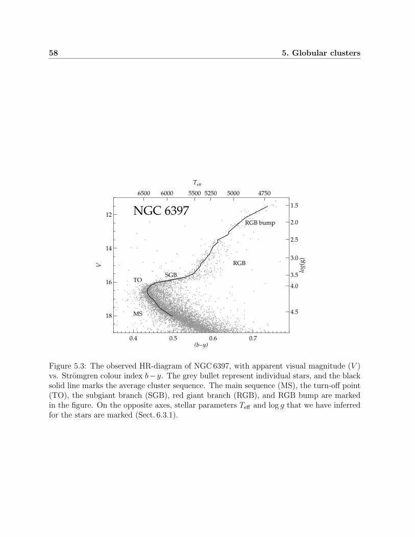
58 5. Globular clusters
0.4 0.5 0.6 0.7(b−y)
18
16
14
12
V
6500 6000 5500 5250 5000 4750
Teff
4.5
4.0
3.5
3.0
2.5
2.0
1.5
log(
g)
NGC 6397
MS
TOSGB
RGB
RGB bump
Figure 5.3: The observed HR-diagram of NGC6397, with apparent visual magnitude (V )vs. Stromgren colour index b−y. The grey bullet represent individual stars, and the blacksolid line marks the average cluster sequence. The main sequence (MS), the turn-off point(TO), the subgiant branch (SGB), red giant branch (RGB), and RGB bump are markedin the figure. On the opposite axes, stellar parameters Teff and log g that we have inferredfor the stars are marked (Sect. 6.3.1).
5.4 High-resolution spectroscopy with FLAMES 59
can study the internal processes in detail and thereby constrain the physics of stars bothon microscopic, atomic, scales and the convective and turbulent motions on macroscopicscales.
Obviously, studies that trace the surface evolution of elements through globular clusterstars in different evolutionary phases, would be biased, or maybe even rendered useless,if the basic assumption of a common initial abundance of all stars is falsified. It is thusimportant to carefully investigate this aspect. Especially, the abundance spread amongstars with similar stellar parameters can lend support to, or refute the hypothesis of acommon initial abundance. Such investigations of globular cluster stars have shown arather complex picture: On the one hand, the star-to-star abundance scatter is alwaysvery small in commonly analysed elements like Ca, Ti, and Fe (a notable exception to therule is ω cen), seemingly consistent with the simplistic view. On the other hand, lightspecies like N, O and Na show large star-to-star scatter, incompatible with observationalerrors, and thus clearly disfavour a common initial abundance (see Sect. 7.1 and referencestherein). Rather, it is believed that present-day globular clusters host more than one stellargeneration, with slightly different initial chemical composition of light elements.
In our investigation of signatures of in-situ depletion of Li in dwarfs, subgiants andgiants (Chapter 6), we use Na abundances to distinguish between the different generationsand assess possible bias in the interpretations. In Chapter 7 we focus instead on the detailedchemical compositions of a large number of elements in a sample of giant stars, in orderto investigate closer the origin of multiple population and constrain chemical evolution ofthe cluster as a whole.
5.4 High-resolution spectroscopy with FLAMES
To perform our spectroscopic investigations of the globular cluster NGC 6397, we haveused the fibre-fed, multi-object instrument FLAMES (Pasquini et al., 2002), mounted onVLT-UT2, at ESO Paranal, Chile. This instrument is ideal for medium-to-high resolutionstudies of dense stellar environments, since it is capable of collecting data for > 100 targetssimultaneously, located within a total field-of-view of 25′. This section will describe themost important steps in the observational procedure.
5.4.1 The observational setup
We use the UVES+MEDUSA combined mode of FLAMES. In this mode, eight opticalfibres with 1′′ aperture are fed to the red arm of the high-resolution ultra-violet and visualechelle spectrograph (UVES, Dekker et al. 2000). The standard settings of UVES covera large wavelength region (470–700 nm or 700–1000 nm) with a resolving power of R =47 000. At the same time, 135 individual fibres of 1.2′′ aperture are fed to the GIRAFFEinstrument, with a typical wavelength coverage of 30 nm and a resolving power of R =20 000, in the settings that we used. The fibres are all either allocated to individual starsor placed at random, empty positions around the field-of-view. The latter are so called sky-
60 5. Globular clusters
fibres and intended to sample the light only from background sources, mainly the reflectedmoonlight.
The targeted stars are selected from a photometric catalogue of the cluster. The pho-tometry should be as precise and well calibrated as possible, to allow the fibres to beplaced centrally on the target, thus maximising the number of photons collected by theCCD detector (CCD stands for charged coupled device). The GIRAFFE CCD consistsof roughly 2000 × 4000 pixels, with longer of the two being the dispersion direction. Theechelle orders, one for each fibre and target, lie barely separated from each other along theother direction.
5.4.2 Data reduction and processing
The purpose of the data reduction procedure is to collapse the data from the two-dimensionalCCD format, to a one-dimensional, calibrated spectra for each target. The calibration stepsinvolve transforming the data from pixel to wavelength space, correcting for the varyingsensitivity over the detector, and subtracting background contribution from the instrumentitself (see Fig. 5.4). The manipulation of the science exposure and a number of calibrationframes are performed in the following order:
• Subtraction of bias, which is a background signal dependent on electronics of thesystem. This signal is determined by performing a number of read-outs from zero-time exposures.
• Subtraction of dark current, which is a time-dependent signal stemming from thenon-zero temperature of the detector. This is measured by performing pseudo-observations without exposing the CCD to a light source.
• Determining the order architecture for the given setup, i.e. a model of how the lightis distributed on the detector. This is achieved by exposing the CCD to a bright,continuous, light source with known properties (i.e. a lamp or a white wall) andcreate so called flat fields. The order pattern is masked with fitted polynomials,whose parameters are saved for later use.
• Determining the dispersion solution, i.e. the correlation between pixel and wave-length scale. This is achieved by exposing the CCD with the light from a lamp con-taining excited noble gas particles (thorium and argon). The detected signal showsnarrow emission lines with known wavelengths, and can thus be used for calibration.
• The science frame is divided by a normalised flat field frame, which corrects the datafor various instrumental artifacts such as the inhomogeneous illumination, dust onthe optical system, varying sensitivity over the detector etc.
• The order architecture is used to extract the two-dimensional data from the scienceframe, and convert them to one dimension, simply by summing up the signal acrosseach individual order.
5.5 Determination of stellar parameters 61
Fig 5.4 shows a cross-section along the order direction of the GIRAFFE CCD plate, andillustrates the detected signal of science and calibration frames at a specific wavelength.
Once the observed data are in the format of one-dimensional spectra of stars and skypositions, some further processing is needed before the abundance analysis can start. First,the sky-spectra are averaged and the mean signal is subtracted from the stellar spectra.Second, the Doppler shift caused by the movement of the star relative to the telescope atthe time of observation, is corrected for by identifying absorption lines in the spectrum.Usually we collected multiple exposures of each star, 3 and once they are all brought tothe same local rest frame, they are coadded to improve the quality. At the same time,outlying pixel values are removed, such as pixels affected by cosmic ray hits. Figs. 6.4 and7.2 show examples of the final product.
5.5 Determination of stellar parameters
As discussed in Sect. 1.2, it is necessary to determine a number of fundamental stellar pa-rameters to infer elemental abundances. In particular, we need to estimate the effectivetemperature Teff and the surface gravity log(g) of all our stars. In the following we intro-duce the methods used to determine these parameters, and discuss some advantages anddisadvantages.
5.5.1 Effective temperature
Especially for the determination of the Li abundance, an accurate estimate of Teff is veryimportant. We adopt three different methods to this end, based on different photometricand spectroscopic observables.
Photometry
Given that the continuous flux spectrum emitted by a star has the approximate shape ofa black-body, it is easily realised that colours, i.e. differences between the flux sampledin different wavelength regions, can be used as temperature indicators. Analogously toWien’s displacement law for black-body radiation (λmax ∝ T−1), the flux peak is locatedat shorter wavelength, the higher the effective temperature of the star (the solar spectrumpeaks at ∼ 450 nm).
To translate between colour and effective temperature, we use calibrated scaling rela-tions obtained by empirical or theoretical means. The relations derived by (Alonso et al.,1996, 1999; Ramırez & Melendez, 2005; Casagrande et al., 2010) are calibrated on the socalled infra-red flux method (IRFM). The essence of this technique lies is obtaining theapparent bolometric flux for a large calibration sample, and use the ratio between the
3This is simply done for practical purposes. If the CCD is exposed for too long without interruption,it is more badly affected by cosmic rays. Also, external conditions may change rapidly, and thus decreasethe quality of the collected signal or even render it useless.

62 5. Globular clusters
1500 1550 1600 1650 1700Pixel
100
101
102
103
104
105
Sig
nal
FlatScience exposureBiasDark
Figure 5.4: Cross-section along the order direction of the GIRAFFE CCD. The exposuretype is indicated with labels. Only the stellar spectra can be clearly identified in the scienceexposure. Some of the orders that appear to be without signal are pointed to sky positions.
5.5 Determination of stellar parameters 63
bolometric flux (∝ T 4eff) and the the flux measured at a specific reference wavelength in the
near infra-red (∝ Teff). This ratio remains highly sensitive to Teff , while independent ofe.g. the distance to the star. Having derived the effective temperatures of the calibrationsample through the IRFM, the mentioned studies present polynomial fits between Teff anda variety of different colour indices. A great advantage with this method is that it is fairlymodel independent, and we have only to ensure that the calibration is appropriate for thecolour ranges, metallicities, and surface gravities spanned by our targets. In addition to theIRFM calibrations, we have used the colour-Teff relations derived by Onehag et al. (2009).These rely solely on synthetic colours, computed using atmospheric models (Gustafssonet al., 2008). The good agreement between the two is indeed reassuring (Sect. 6.3.1).
Spectroscopy
Effective temperatures can also be estimated directly from the stellar spectrum, which con-trary to photometric methods, is independent on the assumed value of the ’reddening’. Theabsolute flux needed to compute colours may be significantly affected by light-absorbingdust particles residing in gas clouds in the line-of-sight towards the star. This is called red-dening, since the bluer wavelengths are more efficiently scattered by dust thereby makingthe star appear more red. Spectroscopic techniques, on the other hand, rely on the relativeflux of spectral lines and continuum, and are therefore not affected by reddening.
As described in Sect. 6.3.1, we derive Teff by fitting a LTE synthetic spectrum to theobserved Hα line profile. This spectral line originates from the bound-bound transitionbetween the first and second excited state of neutral hydrogen (n = 2−3). The populationof the first excited state of H I has a large temperature sensitivity in late-type stars, whilethe sensitivity to surface gravity and metallicity are small, making Hα and other Balmerlines suitable Teff-indicators. Obviously, the method is still model dependent to a certainextent, especially on the convection parameters of the model atmosphere (see Chapter 1),but also on the LTE assumption for the hydrogen level populations (see e.g. Barklem2007b; Pereira et al. submitted). In addition, the hydrogen lines are broad features inthese stars, and a reliable flat-fielding (Sect. 5.4.2) of the observed spectrum is critical torecover the true line shape (Korn et al., 2007).
Finally, we have also inferred effective temperatures from the LTE excitation equilib-rium of Fe I. This atom has numerous spectral lines in the observed stars, originating fromatomic states with a range of different excitation energies (0 − 5 eV). Therefore, if thetemperature structure of the model is wrong, the abundances based on individual lines willshow a systematic trend with the excitation potential of the lower level involved in thetransition. By fine-tuning the effective temperature of the model, the abundances can bereconciled and the trend flattened. This technique may give very precise relative effectivetemperatures, especially if large number of lines are accessible. Further, it is advanta-geous that it is not sensitive to either reddening nor the detailed shape of the continuum.However, also this method is highly dependent on the model atmosphere and the LTEassumption. Even if a flat excitation equilibrium can be established, there is no guaranteethat the inferred Teff is correct, due to possible systematic errors in the modelling procedure
64 5. Globular clusters
that have a differential impact on level populations of different excitation energies.To conclude, all methods have their individual pros and cons and we chose to adopt a
photometric Teff-scale for all stars, mainly to make the analysis as homogeneous as possible.Our observations did not cover any Balmer lines for the hottest targets, nor did the spectracollected for these stars contain enough iron lines to establish the excitation equilibrium. Inaddition, we could minimise the impact of possible patchy reddening over the field-of-viewby relying on fiducial colour-magnitude sequences (Sect. 6.2.2).
5.5.2 Surface gravity
Once the effective temperature has been determined, the surface gravity can be found byusing the relations L = 4πR2F = 4πR2σT 4
eff , g = GM/R2 and the definition of absolutebolometric magnitude (Sect. 5.1). After some simplifications, we obtain for g in cgs units[cm/s2]:
log g = −12.51 + log M/M + 0.4×Mbol + 4× log Teff (5.1)
In addition to Teff , it is thus necessary to have estimates of the stellar mass and theabsolute bolometric magnitude. The former is determined from stellar evolution models,assuming a certain age (13.5Gyr) and chemical composition of the cluster stars. Theexact values are not critical, since the mass-dependence is comparably weak. The absolutebolometric magnitude is obtained from the observed (apparent) visual magnitude V , anestimate of the so called distance modulus (V −MV = 12.57), as well as the bolometriccorrection. The distance modulus can be inferred by comparing the observed colour-magnitude diagram to photometry of field stars with similar properties and distances thatare known through parallax measurements 4. For NGC6397, this has been done using theupper MS and SGB (12.58± 0.08, Gratton et al. 2003) and dwarfs of spectral type M onthe lower MS (12.13 − 12.24, Reid & Gizis 1998). Finally, the bolometric correction isobtained from Teff and [Fe/H], using the empirical calibration by Alonso et al. (1999).
There are also spectroscopic techniques to infer surface gravity, which we explore inSect. 7.3.5. The most common method is to make use of the electron density-dependenceof the ionisation equilibrium of iron (see Eq. 1.2). An LTE atmosphere of low surfacegravity and electron density (Pe ∝ gk, where k ≈ 1/3...2/3, Gray 2005) has a higherfraction of singly ionised iron compared to neutral. If the surface gravity of the model isincorrect, the iron abundance inferred from Fe I will show a systematic offset from thoseinferred from Fe II lines. Again, by reconciling the two species we obtain an estimate oflog g, containing a more or less severe bias due to the simplifying assumptions of 1D andLTE. In principal, all species with detectable spectral lines from different ionisation stages,such as Ca, Ti, and Cr, can be used to derive the surface gravity.
4The parallax distance is inferred by measuring the apparent movement of the star relative to the fixedpositions of very distant objects, as the Earth orbits around the Sun.
Chapter 6
Signatures of intrinsic Li depletionand Li-Na anti-correlation in themetal-poor globular clusterNGC 6397
The following article was published in Astronomy & Astrophysics in August 2009 (Lind,Primas, Charbonnel, Grundahl, & Asplund). The work is based on data collected atEuropean Southern Observatory (ESO), Paranal, Chile, under program IDs 077.A-0018(A)and 281.D-5028(A), as well as data collected with the Danish 1.54m at European SouthernObservatory (ESO), La Silla. Tables 6.2, 6.3, and 6.4 are only available in electronic format the CDS: http://vizier.u-strasbg.fr/viz-bin/VizieR?-source=J/A+A/503/545.
6.1 Introduction
The detection of Li in the atmospheres of old and metal-poor Population II stars hasopened up an observational link to the primordial Universe. 7Li is indeed one of fourisotopes that were synthesised by nuclear reactions shortly after the Big Bang. With themost recent determination of the baryon density from the 5-year release of WMAP data,Ωbh
2 = 0.02273± 0.00062 (Dunkley et al., 2009), an initial abundance of N(7Li)/N (H) =5.24+0.71
−0.67×10⁻¹⁰ or A(Li) = 2.72±0.061 is obtained from standard Big Bang nucleosynthesis(BBNS) (Cyburt et al., 2008). This is significantly higher than what is found for the “Spiteplateau” (Spite & Spite, 1982) in the Galactic halo, a well-defined Li abundance plateauconsisting of metal-poor halo dwarfs and early SGB stars.
The plateau abundance in the field has been determined in a number of recent studiesto span the range A(Li) ≈ 2.0 − 2.4 for stellar metallicities [Fe/H] = (−3.5) − (−1.0),with a possible tendency toward increasing lithium abundance with increasing metallicity
1A(Li) = log(
N (Li)N (H)
)+ 12
666. Signatures of intrinsic Li depletion and Li-Na anti-correlation in the
metal-poor globular cluster NGC 6397
(Ryan et al., 2001; Melendez & Ramırez, 2004; Charbonnel & Primas, 2005; Asplundet al., 2006; Bonifacio et al., 2007a; Hosford et al., 2009; Aoki et al., 2009). Differencesbetween the various analyses may arise from the choice of effective temperature scale andcorrections for non-LTE effects. It is nevertheless clear that a discrepancy by a factorof 2 − 4 with the cosmological prediction is unavoidable, suggesting that the stars haveundergone the corresponding surface depletion of Li. An important fact is that in allthe recent observational analysis (i.e., 21st century) of halo field stars, no evidence ofsignificant dispersion has been found along the plateau, except for a few stars with strongLi abnormalities (Ryan et al., 1999; Asplund et al., 2006).
Soon after the discovery of the Spite plateau, Michaud et al. (1984) predicted Li de-pletion under the combined action of gravitational settling and weak turbulence in theradiative zones of Population II stars. Using sophisticated stellar models that treat atomicdiffusion and radiative acceleration from first principles, Richard et al. (2005) illustrate howthe comparably low Li value found in old, metal-poor stars could be naturally explained,assuming rather strict limits to the turbulent transport extent and efficiency. However, asof today the nature of the underlying physical mechanism responsible for turbulence hasnot been definitively identified, the main difficulty for the conjectured processes (mass loss,rotation-induced mixing, ...) being to account for the negligible Li dispersion along theplateau.
Charbonnel & Primas (2005) revisited the literature Li data for halo field stars withparticular focus on the evolutionary status of the sample stars. This study discoveredfor the first time that the mean Li value appear to be higher for the TO and SGB starsthan for the dwarfs. This result, together with the finding that all halo stars with Liabnormalities (i.e., strong deficiency or high content) lie on, or originate from, the hotside of the plateau, lead the authors to suggest that the most massive (i.e., post-MS) ofthe halo stars still observable today have had a different Li history than their less massivedwarf counterparts. Charbonnel & Primas (2005) suggested that such a behaviour may bethe signature of a transport process of chemical elements and angular momentum whoseefficiency changes on the blue edge of the plateau. This behaviour corresponds to that of thegeneration and filtering of internal gravity waves in both Population II and I stars (Talon &Charbonnel, 2003; Charbonnel & Talon, 2008). Talon & Charbonnel (2004) describe howinternal gravity waves coupled with rotation-induced mixing are expected to lead to higherLi homogeneity among the plateau dwarf stars than among the more massive, slightlyevolved stars, a scenario which may explain the observational findings by Charbonnel &Primas (2005). Speaking in favour of this model is its ability to simultaneously explain theinternal solar rotation profile and the time evolution of the Li abundance at the surface ofsolar- and F-type stars as seen in Galactic open clusters (Charbonnel & Talon, 2005).
By turning to stars in metal-poor Galactic globular clusters, the intrinsic stellar pro-cesses involved can be further constrained. This approach presents some obvious advan-tages. In particular, the evolutionary status of the observed stars can be determinedunambiguously and, presumably, all stars in a cluster were born with the same metallic-ity (although the surface metallicities observed today may vary between stars in differentevolutionary phases, due to the effects of atomic diffusion Korn et al. 2007; Lind et al.
6.1 Introduction 67
2008).
NGC 6397 is one of the most well-studied metal-poor globular clusters and its Li contenthas been documented down to the magnitude of the cluster TO point in several studies(Pasquini & Molaro, 1996; Castilho et al., 2000; Thevenin et al., 2001; Bonifacio et al.,2002; Korn et al., 2006, 2007), however, with rather poor number statistics. Bonifacioet al. (2002) found A(Li) = 2.34 ± 0.06 for the mean abundance of twelve TO stars,whereas Korn et al. (2007) found 2.24±0.05 for five TO stars and 2.36±0.05 for two SGBstars. By comparing this observed abundance difference of Li (as well as Fe, Ca, Mg, andTi) to predictions from the stellar-structure models by Richard et al. (2005) and referencestherein, Korn et al. (2007) empirically constrain the efficiency of slow macroscopic motionscounteracting atomic diffusion below the convective envelope, which should ultimatelyprovide clues on the origin of turbulence. Note that some slow macroscopic process isalso required to reproduce the observed morphologies of globular cluster colour-magnitudediagrams (VandenBerg et al., 2002).
Interpreting abundance trends in globular clusters must however be done with greatcaution. Indeed, it is well-known that globular-cluster stars present striking anomalies intheir light element content that are not seen among their field counterparts (for reviewssee e.g. Gratton et al. 2004; Charbonnel 2005). More precisely, C, N, O, Na, Mg, andAl abundances show large star-to-star variations within individual clusters. C and N, Oand Na, and Mg and Al are respectively anti-correlated, the abundances of C, O, and Mgbeing depleted in some stars while those of N, Na, and Al are enhanced. Importantly, theabundance of Li was found anti-correlated with that of Na and correlated with that of O inturnoff stars in the more metal-rich globular clusters NGC 6752 and 47 Tuc (Pasquini et al.,2005; Bonifacio et al., 2007b). These abundance patterns are explained by contamination ofthe star-forming gas by hydrogen-processed material ejected by a first generation of short-lived massive globular-cluster stars. This increases the Na abundances while loweringthe O and Li abundances with respect to the pristine cluster composition in a secondgeneration long-lived low-mass stars. In the framework of the self-enrichment scenario theLi content of globular-cluster stars is actually an important tool to quantify the dilutionfactor between the ejecta of the massive stars responsible for pollution and the pristineintra-cluster matter (Prantzos & Charbonnel, 2006; Decressin et al., 2007b,a). Grattonet al. (2001) and Carretta et al. (2005) uncovered rather large variations in both O andNa, anti-correlated with each other, in SGB and dwarf stars in NGC6397 (see also Norris& Da Costa 1995; Castilho et al. 2000 for bright giants). This cluster has thus sufferedfrom internal pollution in its infancy.
In the present study we analyse Li and Na abundances for a large sample of stars inNGC 6397, in an attempt to disentangle the primordial value of Li, with effects of atomicdiffusion and intrinsic stellar depletion on the one hand, and early cluster pollution on theother hand. Sect. 6.2 describes the observations and data reduction, Sect. 6.3 describes thedetermination of stellar parameters and the abundance analysis. In Sect. 6.4 we presentthe Li and Na abundances found, and in Sect. 6.5 we discuss signatures of Li depletion inthe cluster. Sect. 6.6 summarises our conclusions.
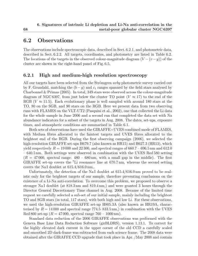
686. Signatures of intrinsic Li depletion and Li-Na anti-correlation in the
metal-poor globular cluster NGC 6397
6.2 Observations
The observations include spectroscopic data, described in Sect. 6.2.1, and photometric data,described in Sect. 6.2.2. All targets, coordinates, and photometry are listed in Table 6.2.The locations of the targets in the observed colour-magnitude diagram (V − (v−y)) of thecluster are shown in the right-hand panel of Fig. 6.5.
6.2.1 High and medium-high resolution spectroscopy
All our targets have been selected from the Stromgren uvby photometric survey carried outby F.Grundahl, matching the (b− y) and c1 ranges spanned by the field stars analysed byCharbonnel & Primas (2005). In total, 349 stars were observed across the colour-magnitudediagram of NGC 6397, from just below the cluster TO point (V ≈ 17) to the end of theRGB (V ≈ 11.5). Each evolutionary phase is well sampled with around 180 stars at theTO, 80 on the SGB, and 90 stars on the RGB. Here we present data from two observingruns with FLAMES on the VLT-UT2 (Pasquini et al., 2002), one that collected the Li datafor the whole sample in June 2006 and a second run that completed the data set with Naabundance indicators for a subset of the targets in Aug. 2008. The dates, set-ups, exposuretimes, and atmospheric conditions are summarised in Table 6.1.
Both sets of observations have used the GIRAFFE+UVES combined mode of FLAMES,with Medusa fibres allocated to the faintest targets and UVES fibres allocated to thebrightest end of the RGB. During the first observing campaign (2006), we selected thehigh-resolution GIRAFFE set-ups H679.7 (also known as HR15) and H627.3 (HR13), whichyield respectively R = 19 000 and 22 300, and spectral ranges of 660.7 – 696.5 nm and 612.0– 640.5 nm. Both settings were observed in combination with the UVES Red 580 setting(R = 47 000, spectral range: 480 – 680 nm, with a small gap in the middle). The firstGIRAFFE set-up covers the 7Li resonance line at 670.7 nm, whereas the second settingcovers the Na I doublet at 615.4/616.0 nm,.
Unfortunately, the detection of the Na I doublet at 615.4/616.0 nm proved to be real-istic only for the brightest targets of our sample, therefore preventing conclusions on theexistence of a Li-Na anti-correlation. To overcome this problem, we proposed to observe astronger Na I doublet (at 818.3 nm and 819.4 nm,) and were granted 3 hours through theDirector General Discretionary Time channel in Aug. 2008. Because of the limited timerequest we carefully selected a sub-set of our initial sample, mainly including the brightestTO and SGB stars (in total, 117 stars), with both high and low Li. For these observations,we used the high-resolution GIRAFFE set-up H805.3A (also known as HR19A, charac-terised by R = 14 000 and spectral range 774.5–833.5 nm,) in combination with the UVESRed 860 set-up (R = 47 000, spectral range 760 – 1000 nm).
Standard data reduction of the 2006 GIRAFFE observations was performed with theGeneva Base Line Data Reduction Software (girBLDRS), version 1.13.1. To correct forthe highly elevated dark current in the upper corner of the old CCD a carefully scaledand smoothed 2D dark-frame was subtracted from each science frame. The 2008 data wereobtained after the GIRAFFE CCD upgrade that took place in Apr. /May 2008 and contain
6.2 Observations 69
negligible dark current. These data were reduced with the ESO GIRAFFE pipeline, version2. 5. 3. UVES data reductions were performed with the FLAMES UVES pipeline, version2. 9. 7.
After initial reduction followed sky-subtraction and radial-velocity correction. Throughradial-velocity measurements we identified six non-members. Furthermore, we disregardedone star that appeared to be too metal-rich to be a cluster member, three stars that clearlyfall off the cluster sequence, and yet three more stars for which the observed spectra are oftoo poor quality. All stars that were rejected are listed with comments in Table 6.2. Theremaining sample consists of 32 stars with spectra obtained with the UVES Red 580 set-up(we hereafter refer to this set as the ’UVES sample’) and 284 stars with spectra obtainedwith the GIRAFFE H679.7 and H627.3 set-ups. The UVES sample and the GIRAFFEsample have 11 stars in common. A sub-sample of eight stars were observed in the UVESRed 860 set-up and 117 with the GIRAFFE H805.3A set-up. The UVES sample andGIRAFFE sample have two stars in common.
The mean barycentric radial velocity obtained for all cluster members is 18.5±0.2 km s−1,in good agreement with Lind et al. (2008) (18.1 ± 0.3 km s−1) and Milone et al. (2006)(18.36± 0.09(±0.10) km s−1).
6.2.2 Stromgren photometry
The Stromgren uvby photometry employed for this investigation was obtained at the Danish1.54m telescope on La Silla, Chile, and is identical to the data set used by Korn et al. (2007);Lind et al. (2008). We reiterate the main points here. All uvby observations were collectedduring a two week run in May 1997, with a large number of observations of standard starsobserved on the photometric nights. The field covered is roughly 9′ in diameter and slightlywest of the cluster centre. For the photometric reductions we used the same programs andprocedures as described in Grundahl et al. (1998, 1999, 2000, 2002b). The photometriczero points in vby have errors of approximately 0.m01.
The observed (b − y), (v − y), and c1 colours were corrected for the reddening ofNGC 6397, using the relations Eb−y = 0.74 × EB−V , Ev−y = 1.70 × Eb−y, and Ec1 =0.20×Eb−y (Crawford, 1975). We adopted a value of 0.179 for EB−V , following Anthony-Twarog & Twarog (2000), and 12.57 for the cluster distance modulus. The observed coloursof our targets show a spread around the cluster sequence, of the order of 2.2% for (v − y)and larger, 3.7%, for (b − y). To reduce the uncertainty in the photometric colours weconstructed colour-magnitude fiducials for the cluster, as described in Korn et al. (2007);Lind et al. (2008). The observed colour is interpolated at constant V -magnitude ontothe fiducial sequence. The main advantage of using this method is that relative effectivetemperatures are more precisely determined, which in turn lowers the spread in chemicalabundances.
706. Signatures of intrinsic Li depletion and Li-Na anti-correlation in the
metal-poor globular cluster NGC 6397
0.8 1.0 1.2 1.4(v−y)0
4500
5000
5500
6000
6500
Teff [
K]
RM05A9699O09
0.3 0.4 0.5 0.6(b−y)0
Figure 6.1: The (b− y)− Teff and (v − y)− Teff relations considered in the analysis. Thevertical lines mark the area that is linearly interpolated (see text). The scale by Onehaget al. (2009, O09) for pre-TO stars fall above the one for post-TO stars and vice verse forthe scale by Alonso et al. (1996, 1999, A9699). The scale by Ramırez & Melendez (2005,RM05) is the same for pre- and post-TO stars.
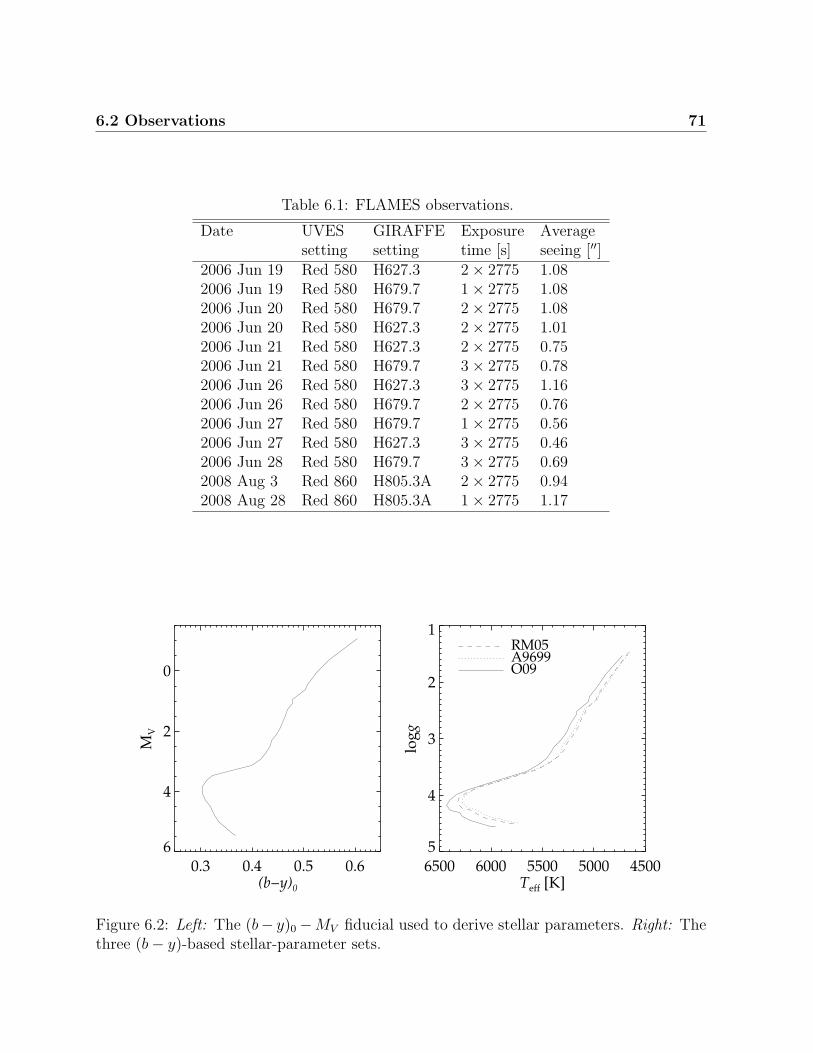
6.2 Observations 71
Table 6.1: FLAMES observations.
Date UVES GIRAFFE Exposure Averagesetting setting time [s] seeing [′′]
2006 Jun 19 Red 580 H627.3 2× 2775 1.082006 Jun 19 Red 580 H679.7 1× 2775 1.082006 Jun 20 Red 580 H679.7 2× 2775 1.082006 Jun 20 Red 580 H627.3 2× 2775 1.012006 Jun 21 Red 580 H627.3 2× 2775 0.752006 Jun 21 Red 580 H679.7 3× 2775 0.782006 Jun 26 Red 580 H627.3 3× 2775 1.162006 Jun 26 Red 580 H679.7 2× 2775 0.762006 Jun 27 Red 580 H679.7 1× 2775 0.562006 Jun 27 Red 580 H627.3 3× 2775 0.462006 Jun 28 Red 580 H679.7 3× 2775 0.692008 Aug 3 Red 860 H805.3A 2× 2775 0.942008 Aug 28 Red 860 H805.3A 1× 2775 1.17
0.3 0.4 0.5 0.6(b−y)0
6
4
2
0
MV
6500 6000 5500 5000 4500Teff [K]
5
4
3
2
1
log
g
RM05A9699O09
Figure 6.2: Left: The (b− y)0−MV fiducial used to derive stellar parameters. Right: Thethree (b− y)-based stellar-parameter sets.
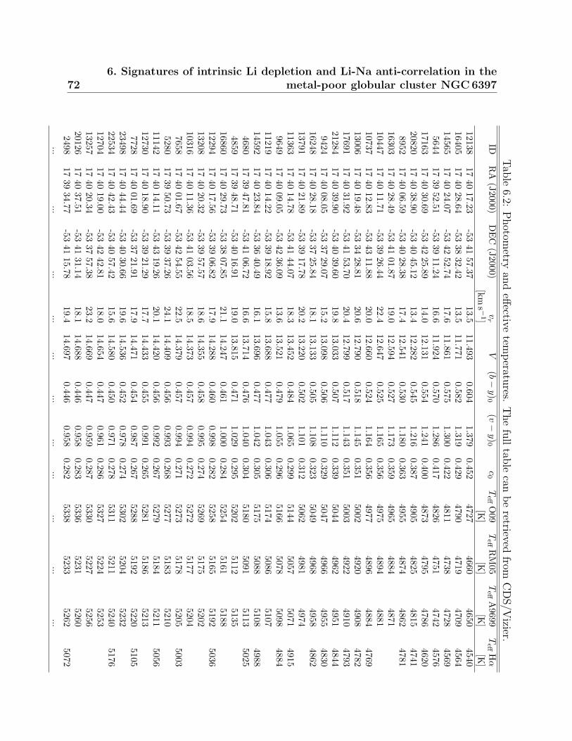
726. Signatures of intrinsic Li depletion and Li-Na anti-correlation in the
metal-poor globular cluster NGC 6397
Tab
le6.2:
Photom
etryan
deff
ectivetem
peratu
res.T
he
full
table
canbe
retrievedfrom
CD
S/V
izier.ID
RA
(J2000)D
EC
(J2000)v
rV
(b−y)
0(v−
y)0
c0
Teff
O09
Teff
RM
05T
eff
A9699
Teff
Hα
[kms −
1][K
][K
][K
][K
]12138
1740
17.23-53
4157.37
13.511.493
0.6041.379
0.4524727
46604650
454016405
1740
28.64-53
3832.42
13.511.771
0.5821.319
0.4294790
47194709
456414565
1740
24.07-53
4252.74
17.611.861
0.5751.300
0.4224811
47384728
45695644
1739
52.51-53
3911.24
16.611.924
0.5701.286
0.4174826
47514742
457617163
1740
30.69-53
4225.89
14.012.131
0.5541.241
0.4004873
47954786
462020820
1740
38.90-53
4045.12
13.412.282
0.5451.216
0.3874905
48254815
47418952
1740
06.59-53
4028.38
17.412.541
0.5301.180
0.3634955
48744862
478116303
1740
28.49-53
4101.87
19.012.594
0.5271.173
0.3594965
48844871
1044717
4011.71
-5339
26.4422.4
12.6470.525
1.1650.356
49754894
488110737
1740
12.83-53
4311.88
20.012.660
0.5241.164
0.3564977
48964884
476913006
1740
19.48-53
3428.81
20.612.790
0.5181.145
0.3515002
49204908
478217691
1740
31.92-53
4153.70
20.412.799
0.5171.143
0.3515003
49224910
479321284
1740
39.90-53
4039.60
19.813.033
0.5071.112
0.3395044
49624951
48449424
1740
08.05-53
3729.07
15.213.098
0.5061.110
0.3295047
49664955
483016248
1740
28.18-53
3725.84
18.113.133
0.5051.108
0.3235049
49684958
486213791
1740
21.89-53
3917.78
20.213.220
0.5021.101
0.3125062
49814974
1136317
4014.78
-5341
44.0718.3
13.4520.484
1.0650.299
51445057
50714915
964917
4009.05
-5342
36.0913.6
13.5210.479
1.0550.296
51665078
50984884
1121917
4014.22
-5339
18.9215.8
13.6880.477
1.0430.306
51745086
510714592
1740
23.84-53
3640.49
16.113.696
0.4771.042
0.3055175
50885108
49884680
1739
47.81-53
4106.72
16.613.714
0.4761.040
0.3045180
50915113
50254859
1739
48.71-53
4016.91
19.013.815
0.4711.029
0.2955202
51125135
1686017
4029.73
-5338
07.8521.1
14.2470.461
1.0000.284
52545161
518812294
1740
17.56-53
3906.82
17.914.288
0.4600.998
0.2825258
51655192
503613208
1740
20.32-53
3957.57
18.614.355
0.4580.995
0.2745269
51755202
1031617
4011.36
-5341
03.5618.5
14.3730.457
0.9940.272
52725177
52047658
1740
01.67-53
4254.55
22.514.379
0.4570.994
0.2715273
51785205
50035280
1739
50.73-53
3937.26
24.114.409
0.4560.993
0.2685277
51835210
1114217
4014.11
-5343
19.2620.1
14.4200.456
0.9920.267
52795184
52115056
1273017
4018.90
-5339
21.2917.7
14.4330.455
0.9910.265
52815186
52137728
1740
01.69-53
3721.91
17.914.471
0.4540.987
0.2675288
51925220
510523498
1740
44.44-53
4030.66
19.614.536
0.4520.978
0.2745302
52045232
2253417
4042.43
-5340
57.4215.6
14.5800.450
0.9710.278
53115211
52405176
1270417
4019.00
-5342
42.8118.0
14.6540.447
0.9610.286
53275224
525313257
1740
20.34-53
3757.38
23.214.669
0.4470.959
0.2875330
52275256
2012617
4037.51
-5341
31.1418.1
14.6880.446
0.9580.283
53365231
52602498
1739
34.77-53
4115.78
19.414.697
0.4460.958
0.2825338
52335262
5072...
......
......
......
......
......
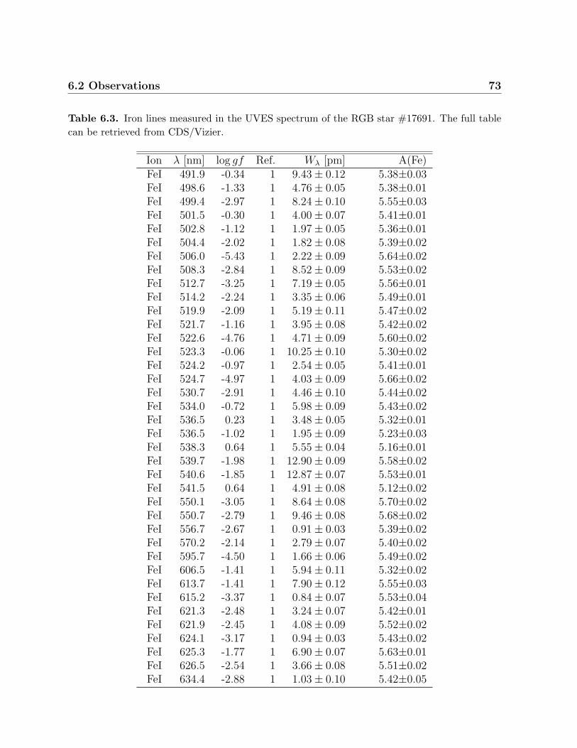
6.2 Observations 73
Table 6.3. Iron lines measured in the UVES spectrum of the RGB star #17691. The full tablecan be retrieved from CDS/Vizier.
Ion λ [nm] log gf Ref. Wλ [pm] A(Fe)FeI 491.9 -0.34 1 9.43± 0.12 5.38±0.03FeI 498.6 -1.33 1 4.76± 0.05 5.38±0.01FeI 499.4 -2.97 1 8.24± 0.10 5.55±0.03FeI 501.5 -0.30 1 4.00± 0.07 5.41±0.01FeI 502.8 -1.12 1 1.97± 0.05 5.36±0.01FeI 504.4 -2.02 1 1.82± 0.08 5.39±0.02FeI 506.0 -5.43 1 2.22± 0.09 5.64±0.02FeI 508.3 -2.84 1 8.52± 0.09 5.53±0.02FeI 512.7 -3.25 1 7.19± 0.05 5.56±0.01FeI 514.2 -2.24 1 3.35± 0.06 5.49±0.01FeI 519.9 -2.09 1 5.19± 0.11 5.47±0.02FeI 521.7 -1.16 1 3.95± 0.08 5.42±0.02FeI 522.6 -4.76 1 4.71± 0.09 5.60±0.02FeI 523.3 -0.06 1 10.25± 0.10 5.30±0.02FeI 524.2 -0.97 1 2.54± 0.05 5.41±0.01FeI 524.7 -4.97 1 4.03± 0.09 5.66±0.02FeI 530.7 -2.91 1 4.46± 0.10 5.44±0.02FeI 534.0 -0.72 1 5.98± 0.09 5.43±0.02FeI 536.5 0.23 1 3.48± 0.05 5.32±0.01FeI 536.5 -1.02 1 1.95± 0.09 5.23±0.03FeI 538.3 0.64 1 5.55± 0.04 5.16±0.01FeI 539.7 -1.98 1 12.90± 0.09 5.58±0.02FeI 540.6 -1.85 1 12.87± 0.07 5.53±0.01FeI 541.5 0.64 1 4.91± 0.08 5.12±0.02FeI 550.1 -3.05 1 8.64± 0.08 5.70±0.02FeI 550.7 -2.79 1 9.46± 0.08 5.68±0.02FeI 556.7 -2.67 1 0.91± 0.03 5.39±0.02FeI 570.2 -2.14 1 2.79± 0.07 5.40±0.02FeI 595.7 -4.50 1 1.66± 0.06 5.49±0.02FeI 606.5 -1.41 1 5.94± 0.11 5.32±0.02FeI 613.7 -1.41 1 7.90± 0.12 5.55±0.03FeI 615.2 -3.37 1 0.84± 0.07 5.53±0.04FeI 621.3 -2.48 1 3.24± 0.07 5.42±0.01FeI 621.9 -2.45 1 4.08± 0.09 5.52±0.02FeI 624.1 -3.17 1 0.94± 0.03 5.43±0.02FeI 625.3 -1.77 1 6.90± 0.07 5.63±0.01FeI 626.5 -2.54 1 3.66± 0.08 5.51±0.02FeI 634.4 -2.88 1 1.03± 0.10 5.42±0.05
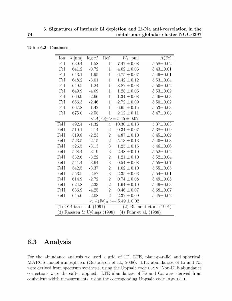
746. Signatures of intrinsic Li depletion and Li-Na anti-correlation in the
metal-poor globular cluster NGC 6397
Table 6.3. Continued.
Ion λ [nm] log gf Ref. Wλ [pm] A(Fe)FeI 639.4 -1.58 1 7.47± 0.08 5.58±0.02FeI 641.2 -0.72 1 4.02± 0.06 5.43±0.01FeI 643.1 -1.95 1 6.75± 0.07 5.49±0.01FeI 648.2 -3.01 1 1.42± 0.12 5.53±0.04FeI 649.5 -1.24 1 8.87± 0.08 5.50±0.02FeI 649.9 -4.69 1 1.28± 0.06 5.63±0.02FeI 660.9 -2.66 1 1.34± 0.08 5.46±0.03FeI 666.3 -2.46 1 2.72± 0.09 5.50±0.02FeI 667.8 -1.42 1 6.65± 0.15 5.53±0.03FeI 675.0 -2.58 1 2.12± 0.11 5.47±0.03
< A(Fe)I >= 5.45± 0.02FeII 492.4 -1.32 4 10.30± 0.13 5.37±0.03FeII 510.1 -4.14 2 0.34± 0.07 5.38±0.09FeII 519.8 -2.23 2 4.87± 0.10 5.45±0.02FeII 523.5 -2.15 2 5.13± 0.13 5.40±0.03FeII 526.5 -3.13 3 1.25± 0.15 5.46±0.06FeII 528.4 -3.19 3 2.48± 0.10 5.52±0.02FeII 532.6 -3.22 2 1.21± 0.10 5.52±0.04FeII 541.4 -3.64 3 0.54± 0.08 5.55±0.07FeII 542.5 -3.37 2 1.02± 0.10 5.55±0.05FeII 553.5 -2.87 3 2.35± 0.03 5.54±0.01FeII 614.9 -2.72 2 0.74± 0.08 5.49±0.05FeII 624.8 -2.33 2 1.64± 0.10 5.49±0.03FeII 636.9 -4.25 2 0.46± 0.07 5.68±0.07FeII 645.6 -2.08 2 2.37± 0.09 5.45±0.02
< A(Fe)II >= 5.49± 0.02(1) O’Brian et al. (1991) (2) Biemont et al. (1991)(3) Raassen & Uylings (1998) (4) Fuhr et al. (1988)
6.3 Analysis
For the abundance analysis we used a grid of 1D, LTE, plane-parallel and spherical,MARCS model atmospheres (Gustafsson et al., 2008). LTE abundances of Li and Nawere derived from spectrum synthesis, using the Uppsala code bsyn. Non-LTE abundancecorrections were thereafter applied. LTE abundances of Fe and Ca were derived fromequivalent width measurements, using the corresponding Uppsala code eqwidth.
6.3 Analysis 75
6.3.1 Effective temperatures and surface gravities
The cluster uvby-photometry was used to calculate effective temperatures for the wholesample. We implemented a number of different calibrations based on the colour indices(v − y) and (b − y) and c1 . Table 6.2 lists effective temperatures calculated using therelations published in Alonso et al. (1996, 1999); Ramırez & Melendez (2005); Onehaget al. (2009). The first three are calibrated on the infra-red flux method (IRFM), whereasthe last is based on theoretical colours from MARCS model atmospheres (Gustafssonet al., 2008). For all stars we assumed [Fe/H] = −2.0. The IRFM colour-Teff relationsconstructed for MS stars were calibrated on stars with log g >∼ 3.8. We accordingly set alimit in absolute visual magnitude, MV > 3.3, for which the MS calibrations are trusted.Analogously, the giant calibrations were calibrated on stars with log g <∼ 3.5 and we trustthem for MV < 2.8. This leaves a gap on the SGB where no calibration is suitable. In thisrange we interpolated linearly between each dwarf- and giant-calibration pair (see verticallines in Fig. 6.1). To each of the obtained effective-temperature scales we calculated surfacegravities from the relation between surface gravity, effective temperature, stellar mass, andluminosity. The details of the calculations are given in Lind et al. (2008).
Onehag et al. (2009) have calculated synthetic (b − y)-colours for a grid of effectivetemperatures, surface gravities, and metallicities. We interpolated in the grid constructedfor [Fe/H] = −2.0, which spans the parameter-space of the sample (see Fig. 4 in Onehaget al. 2009). The interpolation was done iteratively until the parameters found for eachstar were fully consistent, i.e. the Teff − log g pairs found based on the observed colour arealso constrained by relation to mass and luminosity.
For the 32 RGB stars observed with UVES, we could also derive Hα-based effectivetemperatures, using bsyn. Stark broadening is based on the tabulations by Stehle &Hutcheon (1999) and self-broadening of hydrogen follow Barklem et al. (2000). The fittingmethod is automated and based on metal line-free regions extending up to ±5 nm from theline centre (Lind et al., 2008), avoiding the line core. The wings of the Hα-line become verynarrow high up on the RGB, but some sensitivity to effective temperature remains also forthese stars. With a high S/N -ratio it is possible to constrain Teff also for the coolest starsin our sample.
Figure 6.2 shows a comparison between all (b−y)−Teff and (v−y)−Teff relations. The(b− y)-calibration by Onehag et al. (2009) matches the slope of the corresponding IRFM-based calibrations well, but is offset to higher effective temperatures by approximately100K. However, a recent updated calibration based on the IRFM finds effective tempera-tures that are higher than the existing IRFM calibrations, by similar order of magnitude,at these metallicities (Casagrande et al., 2010). Interestingly, Onehag et al. (2009) predictsslightly higher effective temperatures for dwarfs compared to SGB stars of the same colour,whereas the IRFM scale of Alonso et al. (1996, 1999) has the opposite behaviour (throughthe sensitivity to the c1-index). The interpolation between dwarf and giant calibrationsappears more suitable for the (b− y)-relations. The two (v − y) MS scales are too flat tomatch the slope of the corresponding giant relations well. For this reason we regard the(b − y)-relations as more trustworthy and place greater weight on those. The Hα-based
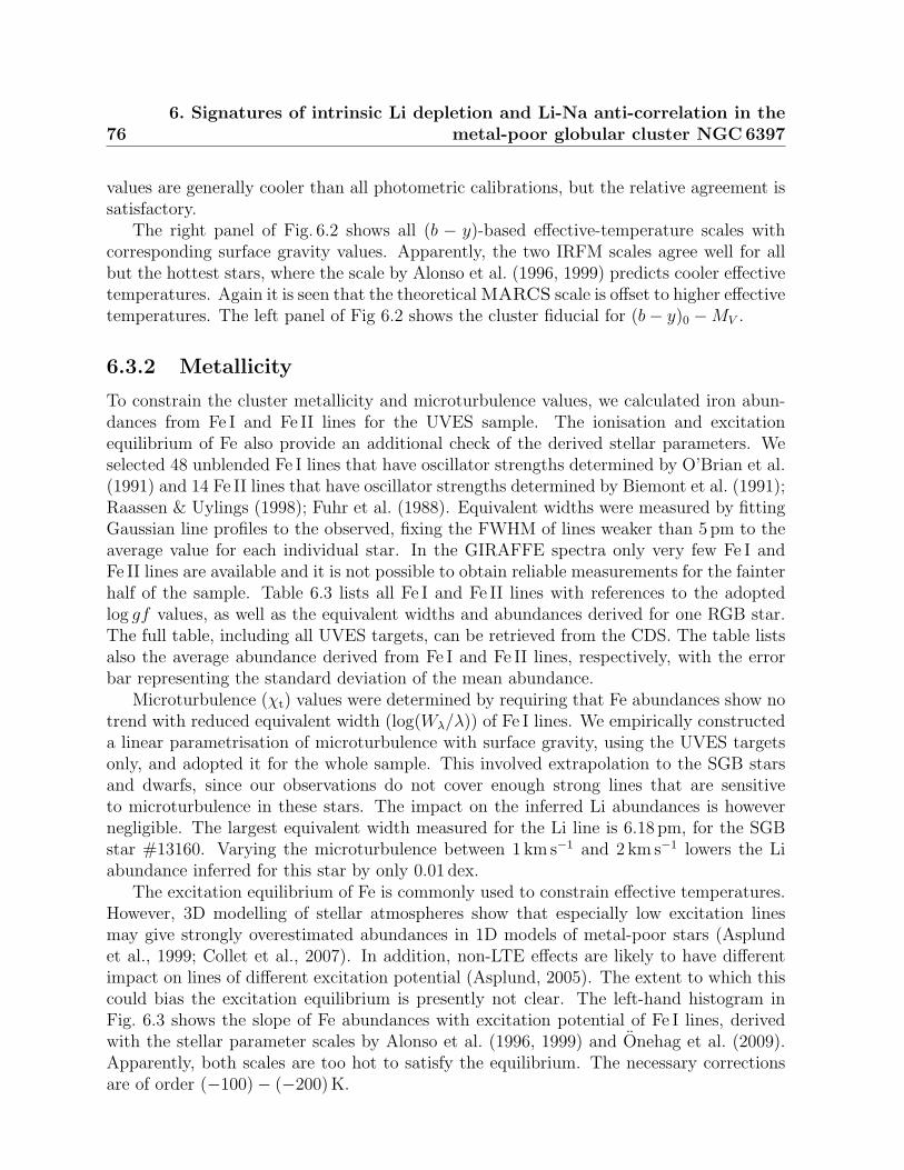
766. Signatures of intrinsic Li depletion and Li-Na anti-correlation in the
metal-poor globular cluster NGC 6397
values are generally cooler than all photometric calibrations, but the relative agreement issatisfactory.
The right panel of Fig. 6.2 shows all (b − y)-based effective-temperature scales withcorresponding surface gravity values. Apparently, the two IRFM scales agree well for allbut the hottest stars, where the scale by Alonso et al. (1996, 1999) predicts cooler effectivetemperatures. Again it is seen that the theoretical MARCS scale is offset to higher effectivetemperatures. The left panel of Fig 6.2 shows the cluster fiducial for (b− y)0 −MV .
6.3.2 Metallicity
To constrain the cluster metallicity and microturbulence values, we calculated iron abun-dances from Fe I and Fe II lines for the UVES sample. The ionisation and excitationequilibrium of Fe also provide an additional check of the derived stellar parameters. Weselected 48 unblended Fe I lines that have oscillator strengths determined by O’Brian et al.(1991) and 14 Fe II lines that have oscillator strengths determined by Biemont et al. (1991);Raassen & Uylings (1998); Fuhr et al. (1988). Equivalent widths were measured by fittingGaussian line profiles to the observed, fixing the FWHM of lines weaker than 5 pm to theaverage value for each individual star. In the GIRAFFE spectra only very few Fe I andFe II lines are available and it is not possible to obtain reliable measurements for the fainterhalf of the sample. Table 6.3 lists all Fe I and Fe II lines with references to the adoptedlog gf values, as well as the equivalent widths and abundances derived for one RGB star.The full table, including all UVES targets, can be retrieved from the CDS. The table listsalso the average abundance derived from Fe I and Fe II lines, respectively, with the errorbar representing the standard deviation of the mean abundance.
Microturbulence (χt) values were determined by requiring that Fe abundances show notrend with reduced equivalent width (log(Wλ/λ)) of Fe I lines. We empirically constructeda linear parametrisation of microturbulence with surface gravity, using the UVES targetsonly, and adopted it for the whole sample. This involved extrapolation to the SGB starsand dwarfs, since our observations do not cover enough strong lines that are sensitiveto microturbulence in these stars. The impact on the inferred Li abundances is howevernegligible. The largest equivalent width measured for the Li line is 6.18 pm, for the SGBstar #13160. Varying the microturbulence between 1 km s−1 and 2 km s−1 lowers the Liabundance inferred for this star by only 0.01 dex.
The excitation equilibrium of Fe is commonly used to constrain effective temperatures.However, 3D modelling of stellar atmospheres show that especially low excitation linesmay give strongly overestimated abundances in 1D models of metal-poor stars (Asplundet al., 1999; Collet et al., 2007). In addition, non-LTE effects are likely to have differentimpact on lines of different excitation potential (Asplund, 2005). The extent to which thiscould bias the excitation equilibrium is presently not clear. The left-hand histogram inFig. 6.3 shows the slope of Fe abundances with excitation potential of Fe I lines, derivedwith the stellar parameter scales by Alonso et al. (1996, 1999) and Onehag et al. (2009).Apparently, both scales are too hot to satisfy the equilibrium. The necessary correctionsare of order (−100)− (−200)K.
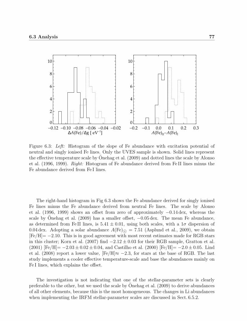
6.3 Analysis 77
−0.12 −0.10 −0.08 −0.06 −0.04 −0.02∆A(Fe)/∆χ [ eV−1]
0
2
4
6
8
10
−0.2 −0.1 0.0 0.1 0.2 0.3A(Fe)II−A(Fe)I
0
2
4
6
8
10
Figure 6.3: Left: Histogram of the slope of Fe abundance with excitation potential ofneutral and singly ionised Fe lines. Only the UVES sample is shown. Solid lines representthe effective temperature scale by Onehag et al. (2009) and dotted lines the scale by Alonsoet al. (1996, 1999). Right: Histogram of Fe abundance derived from Fe II lines minus theFe abundance derived from Fe I lines.
The right-hand histogram in Fig 6.3 shows the Fe abundance derived for singly ionisedFe lines minus the Fe abundance derived from neutral Fe lines. The scale by Alonsoet al. (1996, 1999) shows an offset from zero of approximately −0.14 dex, whereas thescale by Onehag et al. (2009) has a smaller offset, −0.05 dex. The mean Fe abundance,as determined from Fe II lines, is 5.41 ± 0.01, using both scales, with a 1σ dispersion of0.04 dex. Adopting a solar abundance A(Fe) = 7.51 (Asplund et al., 2009), we obtain[Fe/H]= −2.10. This is in good agreement with most recent estimates made for RGB starsin this cluster; Korn et al. (2007) find −2.12± 0.03 for their RGB sample, Gratton et al.(2001) [Fe/H]= −2.03± 0.02± 0.04, and Castilho et al. (2000) [Fe/H]= −2.0± 0.05. Lindet al. (2008) report a lower value, [Fe/H]≈ −2.3, for stars at the base of RGB. The laststudy implements a cooler effective temperature-scale and base the abundances mainly onFe I lines, which explains the offset.
The investigation is not indicating that one of the stellar-parameter sets is clearlypreferable to the other, but we used the scale by Onehag et al. (2009) to derive abundancesof all other elements, because this is the most homogeneous. The changes in Li abundanceswhen implementing the IRFM stellar-parameter scales are discussed in Sect. 6.5.2.
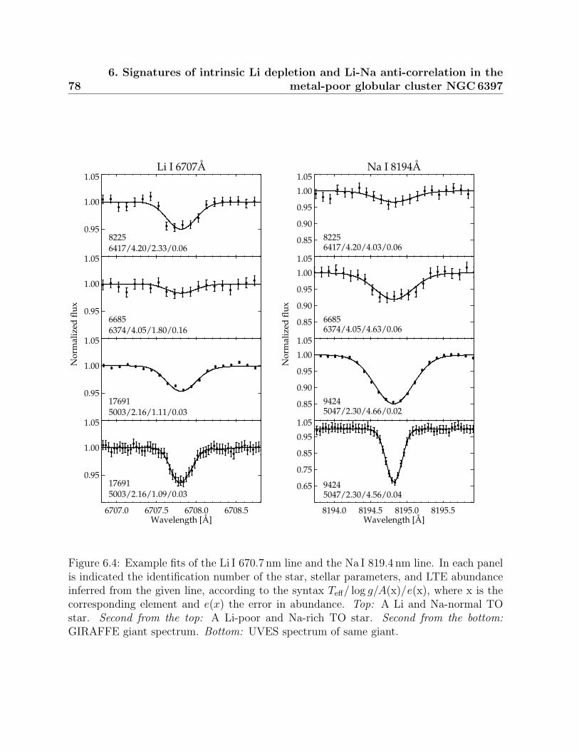
786. Signatures of intrinsic Li depletion and Li-Na anti-correlation in the
metal-poor globular cluster NGC 6397
6707.0 6707.5 6708.0 6708.5Wavelength [Å]
0.95
1.00
1.05
176915003/2.16/1.09/0.03
0.95
1.00
1.05
176915003/2.16/1.11/0.03
0.95
1.00
1.05
66856374/4.05/1.80/0.16
Li I 6707Å
0.95
1.00
1.05
82256417/4.20/2.33/0.06
Nor
mal
ized
flux
Nor
mal
ized
flux
8194.0 8194.5 8195.0 8195.5Wavelength [Å]
0.65
0.75
0.85
0.95
1.05
94245047/2.30/4.56/0.04
0.85
0.90
0.95
1.00
1.05
94245047/2.30/4.66/0.02
0.85
0.90
0.95
1.00
1.05
66856374/4.05/4.63/0.06
Na I 8194Å
0.85
0.90
0.95
1.00
1.05
82256417/4.20/4.03/0.06
Figure 6.4: Example fits of the Li I 670.7 nm line and the Na I 819.4 nm line. In each panelis indicated the identification number of the star, stellar parameters, and LTE abundanceinferred from the given line, according to the syntax Teff/ log g/A(x)/e(x), where x is thecorresponding element and e(x) the error in abundance. Top: A Li and Na-normal TOstar. Second from the top: A Li-poor and Na-rich TO star. Second from the bottom:GIRAFFE giant spectrum. Bottom: UVES spectrum of same giant.

6.3 Analysis 79
6.3.3 Lithium
The 7Li resonance line at 670.7 nm has two fine-structure components, separated only by0.015 nm. At the resolution of GIRAFFE (R = 19300) they are indistinguishable, but asmall line-asymmetry can be seen in the higher-resolution UVES spectra (R = 47000).Accurate measurements of the line require spectrum synthesis (see example fits of the linein Fig.6.4). We adopted log gf = −0.009 and −0.309 for the two components respectively,according to Lindgard & Nielson (1977).
To derive Li LTE abundances for the stars we first normalised each spectrum by it-erative fitting of a first order polynomial, taking into consideration a wavelength regionextending ±0.2 nm from the line centre. Synthetic line profiles were convolved with aGaussian profile to account for the instrumental broadening and broadening due to ro-tation and macroturbulence. The width of the convolving profile was fixed for each starby measurements of single lines of other species. The Li abundance was then varied tofind the best fitting synthetic profile for each star through χ2-minimisation. In total, Liabundances or upper abundance limits could be obtained for 305 stars. Following Norriset al. (2001) and Barklem et al. (2005), errors due to observational uncertainties were es-
timated with the expression: σWλ= λ
√(n)/(R × S/N), where n denotes the number of
pixels spanning the full-width at half maximum for the line, R the spectral resolution, andS/N the signal-to-noise ratio per pixel.
Non-LTE abundance corrections for Li were calculated according to Lind et al. (2009a),a study that is based on calculations on the same MARCS model atmospheres as here(Gustafsson et al., 2008). In contrast to earlier non-LTE analyses (e.g. Carlsson et al.1994; Takeda & Kawanomoto 2005) the study makes use of rigorous quantum mechanicalcalculations (as opposed to the debated but common classical recipes) of cross-sectionsfor collisions with neutral hydrogen, which have influence over the statistical equilibriumof Li. Lind et al. (2009b) show that including the charge transfer reactions between Liand hydrogen in the non-LTE calculations gives abundance corrections that are lower byalmost −0.1 dex for dwarfs at [Fe/H]= −2.0, as compared to neglecting them. For oursample, the MS, TO, and early SGB stars all have non-LTE corrections that are verysimilar, around −0.06 dex. With decreasing effective temperature and surface gravity thecorrections change sign and reach a maximum of +0.13 dex for the coolest RGB star.
6.3.4 Sodium
Sodium abundances or upper abundance limits were derived from the 2008 observationsfor a subset of 117 stars, mainly TO stars and early SGB stars. The abundances werebased on the Na I 818.3 nm and 819.4 nm doublet (when the former was too weak to bedetected, only the latter was used). This doublet is second in strength after the resonancedoublet at 588.5 nm and 589.0 nm, which is strongly affected by interstellar extinction forthe cluster stars and is therefore not useful as abundance indicator. As mentioned above,the 568.2/568.8 nm and 615.4/616.0 nm doublets are too weak to be suitable for abundanceanalysis in the TO region at this metallicity. Despite its unfortunate location in the middle
806. Signatures of intrinsic Li depletion and Li-Na anti-correlation in the
metal-poor globular cluster NGC 6397
of a strong telluric band, the 818.3/819.4 nm Na I doublet does not suffer strongly fromatmospheric blends that would bias the abundance analysis.
The line-fitting method is the same as described for Li and oscillator strengths byKurucz & Peytremann (1975) were adopted. We apply non-LTE abundance correctionsto the 818.3/819.4 nm Na I lines according to Mashonkina et al. (2000)2. The size of thecorrections at this metallicity ranges from −0.14 dex for the hottest, highest surface gravitystars, to approximately −0.31 dex for the coolest giants.
6.3.5 Calcium
For the complete sample of 305 stars, only the equivalent widths of Ca lines 612.2 nm and616.2 nm could be reliably measured. We based the Ca abundance on these two lines for305 stars, adopting oscillator strengths from Smith & O’Neill (1975)
6.4 Results
6.4.1 Li abundances
Table 6.4 lists the adopted stellar parameters, equivalent widths, and abundances. Fig. 6.5shows the Li abundances inferred side-by-side with a colour-magnitude diagram where thespectroscopic targets are marked. In agreement with the expectations (see Sect. 6.1), thereis a rather well defined abundance plateau among the least evolved stars, followed by adrastic drop in Li abundance in the middle of the SGB (MV ≈ 3.3). This pattern is causedby the so-called first dredge-up, i.e., the dilution of the external convective stellar layerswith deeper hydrogen-processed material. A second steep drop occurs at MV ≈ 0.0, whichcorresponds to the luminosity of the RGB bump. A similar decrease in Li abundance hasbeen identified in stars located around the RGB bump in NGC 6752 (Grundahl et al.,2002a) as well as in stars in the halo field (Gratton et al., 2000). Charbonnel & Zahn(2007) describe how this second Li abundance drop can be explained by a mixing processcalled thermohaline convection, which becomes efficient when the hydrogen-burning shellcrosses the chemical discontinuity left behind by the first dredge-up, and which rapidlytransports surface Li down to internal hotter regions where this fragile element burns.
The average Li abundance on the plateau, i.e. only including stars that have not un-dergone dilution due to the first dredge-up (MV > 3.3), is 2.25 ± 0.01, where the error isthe standard deviation of the mean. The 1σ dispersion is 0.09 dex.
2The non-LTE calculations presented in Chapter 2 had not been computed at the time of this analysis.We have verified that the non-LTE corrections by Mashonkina et al. (2000) are very similar to our workfor the specific lines and stellar parameter space
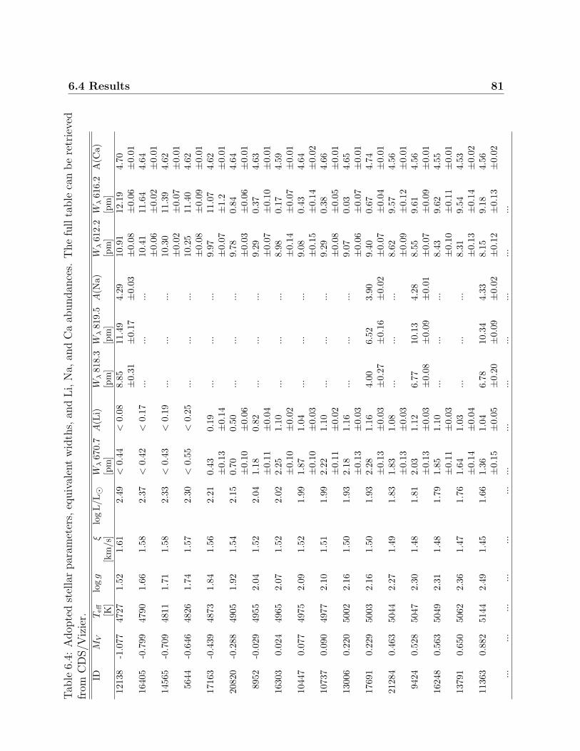
6.4 Results 81
Tab
le6.
4:A
dop
ted
stel
lar
par
amet
ers,
equiv
alen
tw
idth
s,an
dLi,
Na,
and
Ca
abundan
ces.
The
full
table
can
be
retr
ieve
dfr
omC
DS/V
izie
r.ID
MV
Teff
log
gξ
log
L/L
Wλ
670.
7A
(Li)
Wλ
818.
3W
λ81
9.5
A(N
a)W
λ61
2.2
Wλ
616.
2A
(Ca)
[K]
[km
/s]
[pm
][p
m]
[pm
][p
m]
[pm
]12
138
-1.0
7747
271.
521.
612.
49<
0.44
<0.
088.
85±
0.31
11.4
9±
0.17
4.29±
0.03
10.9
1±
0.08
12.1
9±
0.06
4.70±
0.01
1640
5-0
.799
4790
1.66
1.58
2.37
<0.
42<
0.17
...
......
10.4
1±
0.06
11.6
4±
0.02
4.64±
0.01
1456
5-0
.709
4811
1.71
1.58
2.33
<0.
43<
0.19
...
......
10.3
0±
0.02
11.3
9±
0.07
4.62±
0.01
5644
-0.6
4648
261.
741.
572.
30<
0.55
<0.
25...
......
10.2
5±
0.08
11.4
0±
0.09
4.62±
0.01
1716
3-0
.439
4873
1.84
1.56
2.21
0.43±
0.13
0.19±
0.14
......
...9.
97±
0.07
11.0
7±
1.2
4.62±
0.01
2082
0-0
.288
4905
1.92
1.54
2.15
0.70±
0.10
0.50±
0.06
......
...9.
78±
0.03
0.84±
0.06
4.64±
0.01
8952
-0.0
2949
552.
041.
522.
041.
18±
0.11
0.82±
0.04
......
...9.
29±
0.07
0.37±
0.10
4.63±
0.01
1630
30.
024
4965
2.07
1.52
2.02
2.25±
0.10
1.10±
0.02
......
...8.
98±
0.14
0.17±
0.07
4.59±
0.01
1044
70.
077
4975
2.09
1.52
1.99
1.87±
0.10
1.04±
0.03
......
...9.
08±
0.15
0.43±
0.14
4.64±
0.02
1073
70.
090
4977
2.10
1.51
1.99
2.22±
0.11
1.10±
0.02
......
...9.
29±
0.08
0.38±
0.05
4.66±
0.01
1300
60.
220
5002
2.16
1.50
1.93
2.18±
0.13
1.16±
0.03
......
...9.
07±
0.06
0.03±
0.07
4.65±
0.01
1769
10.
229
5003
2.16
1.50
1.93
2.28±
0.13
1.16±
0.03
4.00±
0.27
6.52±
0.16
3.90±
0.02
9.40±
0.07
0.67±
0.04
4.74±
0.01
2128
40.
463
5044
2.27
1.49
1.83
1.83±
0.13
1.08±
0.03
......
...8.
62±
0.09
9.57±
0.12
4.56±
0.01
9424
0.52
850
472.
301.
481.
812.
03±
0.13
1.12±
0.03
6.77±
0.08
10.1
3±
0.09
4.28±
0.01
8.55±
0.07
9.61±
0.09
4.56±
0.01
1624
80.
563
5049
2.31
1.48
1.79
1.85±
0.11
1.10±
0.03
......
...8.
43±
0.10
9.62±
0.11
4.55±
0.01
1379
10.
650
5062
2.36
1.47
1.76
1.64±
0.14
1.03±
0.04
......
...8.
31±
0.13
9.54±
0.14
4.53±
0.02
1136
30.
882
5144
2.49
1.45
1.66
1.36±
0.15
1.04±
0.05
6.78±
0.20
10.3
4±
0.09
4.33±
0.02
8.15±
0.12
9.18±
0.13
4.56±
0.02
......
......
......
......
......
......
...
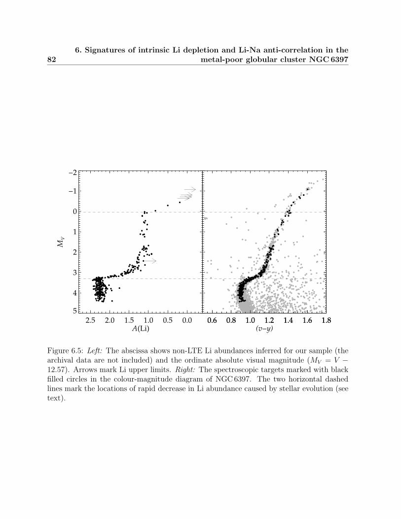
826. Signatures of intrinsic Li depletion and Li-Na anti-correlation in the
metal-poor globular cluster NGC 6397
2.5 2.0 1.5 1.0 0.5 0.0A(Li)
5
4
3
2
1
0
−1
−2
MV
0.6 0.8 1.0 1.2 1.4 1.6 1.8(v−y)
0.6 0.8 1.0 1.2 1.4 1.6 1.8
Figure 6.5: Left: The abscissa shows non-LTE Li abundances inferred for our sample (thearchival data are not included) and the ordinate absolute visual magnitude (MV = V −12.57). Arrows mark Li upper limits. Right: The spectroscopic targets marked with blackfilled circles in the colour-magnitude diagram of NGC 6397. The two horizontal dashedlines mark the locations of rapid decrease in Li abundance caused by stellar evolution (seetext).

6.4 Results 83
6.4.2 Lithium data from the ESO archive
To establish a view of the Li content in NGC6397 that is as complete as possible, we havesearched the ESO archive for observations of more MS, TO, and SGB stars. Especially,to put constraints on the size and significance of a small increase in A(Li) located justbefore the onset of the first dredge-up (see Sect. 6.5.1 and Fig. 6.6) we would benefit fromhaving more stars. In previous analyses, Bonifacio et al. (2002) analyse Li in twelve TOstars (of which seven stars were previously analysed by Thevenin et al. 2001 and threestars by Pasquini & Molaro 1996) and Korn et al. (2007) analyse five TO stars and twoSGB stars. We did not incorporate those stars in our analysis since it would only slightlyhave increased the number statistics. However, we have retrieved and analysed a setof FLAMES archival data from 2007 (079.D-0399(A), P. I. Gonzalez-Hernandez). Theseinclude observations in the GIRAFFE high-resolution set-up H665.0 (HR15N, R = 17000),covering the LiI 670.7 nm line for a sample of 80 dwarfs (MV ≈4.9) and 88 SGB stars(MV ≈ 3.4) in NGC6397. The reduction of the data was performed with the girBLDRSpipeline. In total, 38 MS stars and 55 SGB stars were identified in our uvby photometriccatalogue. For the remaining stars, we add a zero-point correction of 0.09magnitudes tothe visual magnitude scale listed in the archival data, estimated from the targets that werecross-matched between the catalogues. Applying the correction, the two magnitude scalesmatch to typically within 0.02 magnitudes for individual targets. After establishing thevisual magnitudes, colours are assigned to each target by interpolating V onto the fiducialcluster sequences, as was done for the main sample (see Sect. 6.2.2).
The results of the analysis of the archival data are shown together with our own dataset in Fig. 6.6. One more very Li-poor star, marked with an arrow, was identified in thearchive sample, for which only an upper limit to Li could be derived. Especially, the regionaround MV = 3.2 − 3.5 is now much better sampled, with the archival data confirmingthe presence of the small abundance increase just before the steep drop. In addition, theplateau is extended to fainter magnitudes, MV ≈ 5. Including this archive sample wehave Li abundances for 454 stars in the cluster, of which 346 have MV > 3.3. Overallthe qualities of the data sets are similar and the abundances agree very well between thesamples. In total, 14 SGB stars overlap and thus have observations of the Li line in theH665.0 as well as in the H679.7 setting. The mean difference in Li abundance betweenthese 14 stars is −0.02± 0.02 dex, i.e. there is no systematic bias between the data sets.
The average Li abundance on the plateau (i.e., excluding stars with MV < 3.3), includ-ing both our data and the archival data, is 2.270 ± 0.005. Unfortunately Na informationis not available for the archive targets.
6.4.3 The Li-Na anti-correlation
As discussed in Sect. 6.1, globular-cluster samples may suffer from bias due to early pollu-tion of the intra-cluster gas by a first generation of more massive, faster evolving stars. It isthus important to discriminate between first-generation stars that formed out of pure pris-tine material and second-generation stars that formed out of polluted material. The former
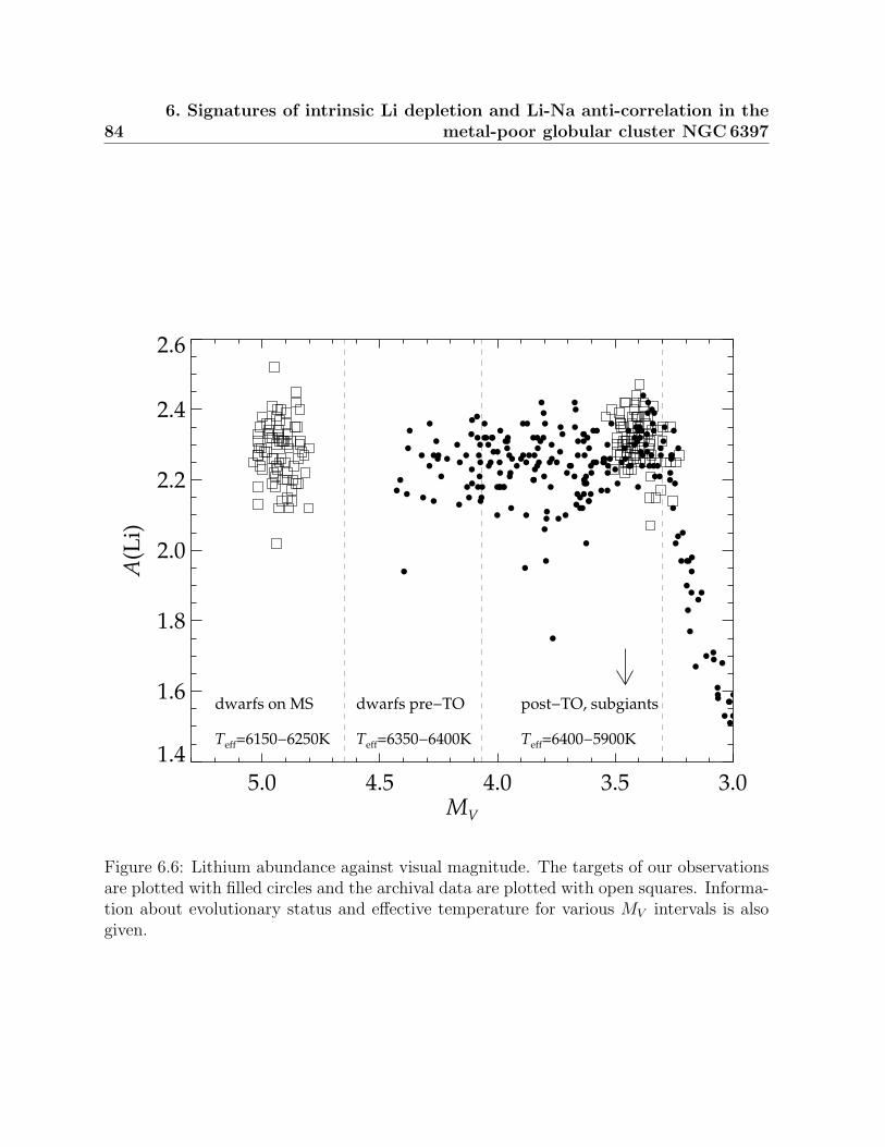
846. Signatures of intrinsic Li depletion and Li-Na anti-correlation in the
metal-poor globular cluster NGC 6397
5.0 4.5 4.0 3.5 3.0M
V
1.4
1.6
1.8
2.0
2.2
2.4
2.6
A(L
i)
dwarfs on MS
Teff=6150−6250K
dwarfs pre−TO
Teff=6350−6400K
post−TO, subgiants
Teff=6400−5900K
Figure 6.6: Lithium abundance against visual magnitude. The targets of our observationsare plotted with filled circles and the archival data are plotted with open squares. Informa-tion about evolutionary status and effective temperature for various MV intervals is alsogiven.
6.4 Results 85
should have been born with the cosmological Li abundance and a low Na-abundance, sim-ilar to that of field stars of comparable overall metallicity. The latter may have inheriteda lower Li abundance at birth and will also exhibit other signatures of H-burning at hightemperature, in particular enhanced Na abundances resulting from the NeNa chain in thepolluter stars.
In Fig. 6.7 we report the Li and Na abundances for 100 stars in our sample with MV >3.3, i.e., those that have not yet undergone Li dilution via the first dredge-up. Note thatit is the first time that these quantities are determined simultaneously for such a largesample of TO and SGB stars in a globular cluster. This diagram clearly emphasises theextent of the star-to-star Na abundance variations (by up to 1 dex) within NGC6397.This is in agreement with the findings by Carretta et al. (2005), which were based on sixdwarfs and nine SGB stars. From the appearance of Fig. 6.7, we deduce that the most Li-poor targets indeed show the most elevated Na levels, implying an anti-correlation betweenthe abundances of Na and Li. The spectrum of the most Li-poor and second most Na-rich star in the sample, #6685, is shown in Fig. 6.4. The abundance pattern displayedby this star and by at least three more stars, agrees well with the globular cluster self-enrichment scenario and we conclude that they have likely been formed from polluted gas.Field stars with similar metallicity to NGC6397 have typical Na abundances in the rangeA(Na) = 3.6 − 3.9 (Andrievsky et al., 2007). It is thus reasonable to regard stars withA(Na) < 3.9 as belonging to a first generation of non-polluted objects.
To find the statistical significance of the indicated Li-Na anti-correlation we performedlinear regression between N(Li)/N (H) and N(Na)/N (H), taking into account measurementerrors in both quantities as well as upper limits on Na (IDL-routine linmix err, seeKelly 2007). The analysis gave a correlation coefficient of −0.6 between the Na and Liabundances, which for a sample of this size is highly significant. The probability of twouncorrelated variables producing such a correlation coefficient is less than 0.05%. However,as can be realised from Fig. 6.7, the significance of the anti-correlation is dependent on themost Na-enhanced stars. In fact, performing the same linear regression for stars withA(Na) < 4.1 no significant anti-correlation was found. The Li abundances among theplateau stars are thus not much affected by high degrees of pollution.
In Fig. 6.7 it is also indicated with a tilted arrow approximately how the location of astar would be affected by an erroneous effective temperature. An error of ∆Teff = ±100Kcorresponds to ∆A(Li) = ±0.07 and ∆A(Na) = ±0.04. Errors in effective temperaturetherefore weakly correlate the abundances with each other, rather than anti-correlate them.Hence, it is clear that the anti-correlation itself is not an artifact from uncertainties in thestellar-parameter determination. Possibly even a tighter anti-correlation exists for all tar-gets, but is being distorted by the tendency of effective-temperature errors to align theabundances. As the Li abundance as well as the Na abundance are based on lines fromneutral atoms, the effective temperature is the stellar parameter with by far the greatest in-fluence over the results. The uncertainties stemming from surface gravity, microturbulence,and metallicity are all negligible in the context.
The extent of the Li and Na variations found in the present study is similar to that foundin NGC 6752 (Pasquini et al., 2005) and 47 Tuc (Bonifacio et al., 2007b), and thus appears
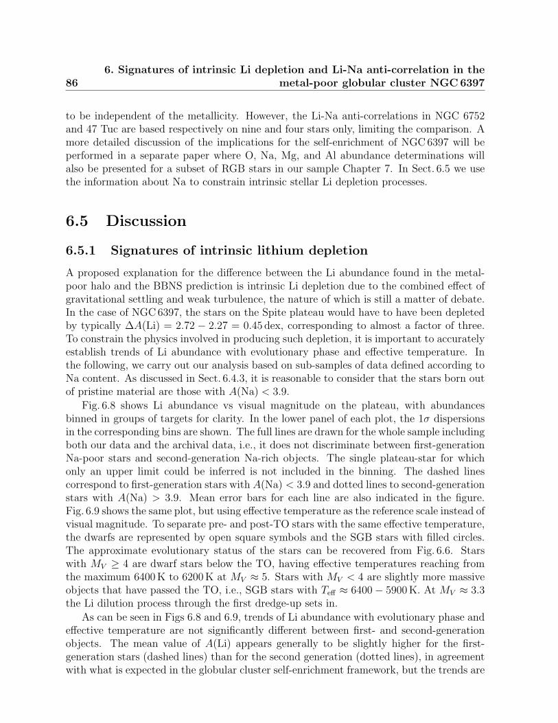
866. Signatures of intrinsic Li depletion and Li-Na anti-correlation in the
metal-poor globular cluster NGC 6397
to be independent of the metallicity. However, the Li-Na anti-correlations in NGC 6752and 47 Tuc are based respectively on nine and four stars only, limiting the comparison. Amore detailed discussion of the implications for the self-enrichment of NGC6397 will beperformed in a separate paper where O, Na, Mg, and Al abundance determinations willalso be presented for a subset of RGB stars in our sample Chapter 7. In Sect. 6.5 we usethe information about Na to constrain intrinsic stellar Li depletion processes.
6.5 Discussion
6.5.1 Signatures of intrinsic lithium depletion
A proposed explanation for the difference between the Li abundance found in the metal-poor halo and the BBNS prediction is intrinsic Li depletion due to the combined effect ofgravitational settling and weak turbulence, the nature of which is still a matter of debate.In the case of NGC6397, the stars on the Spite plateau would have to have been depletedby typically ∆A(Li) = 2.72 − 2.27 = 0.45 dex, corresponding to almost a factor of three.To constrain the physics involved in producing such depletion, it is important to accuratelyestablish trends of Li abundance with evolutionary phase and effective temperature. Inthe following, we carry out our analysis based on sub-samples of data defined according toNa content. As discussed in Sect. 6.4.3, it is reasonable to consider that the stars born outof pristine material are those with A(Na) < 3.9.
Fig. 6.8 shows Li abundance vs visual magnitude on the plateau, with abundancesbinned in groups of targets for clarity. In the lower panel of each plot, the 1σ dispersionsin the corresponding bins are shown. The full lines are drawn for the whole sample includingboth our data and the archival data, i.e., it does not discriminate between first-generationNa-poor stars and second-generation Na-rich objects. The single plateau-star for whichonly an upper limit could be inferred is not included in the binning. The dashed linescorrespond to first-generation stars with A(Na) < 3.9 and dotted lines to second-generationstars with A(Na) > 3.9. Mean error bars for each line are also indicated in the figure.Fig. 6.9 shows the same plot, but using effective temperature as the reference scale instead ofvisual magnitude. To separate pre- and post-TO stars with the same effective temperature,the dwarfs are represented by open square symbols and the SGB stars with filled circles.The approximate evolutionary status of the stars can be recovered from Fig. 6.6. Starswith MV ≥ 4 are dwarf stars below the TO, having effective temperatures reaching fromthe maximum 6400K to 6200K at MV ≈ 5. Stars with MV < 4 are slightly more massiveobjects that have passed the TO, i.e., SGB stars with Teff ≈ 6400− 5900K. At MV ≈ 3.3the Li dilution process through the first dredge-up sets in.
As can be seen in Figs 6.8 and 6.9, trends of Li abundance with evolutionary phase andeffective temperature are not significantly different between first- and second-generationobjects. The mean value of A(Li) appears generally to be slightly higher for the first-generation stars (dashed lines) than for the second generation (dotted lines), in agreementwith what is expected in the globular cluster self-enrichment framework, but the trends are
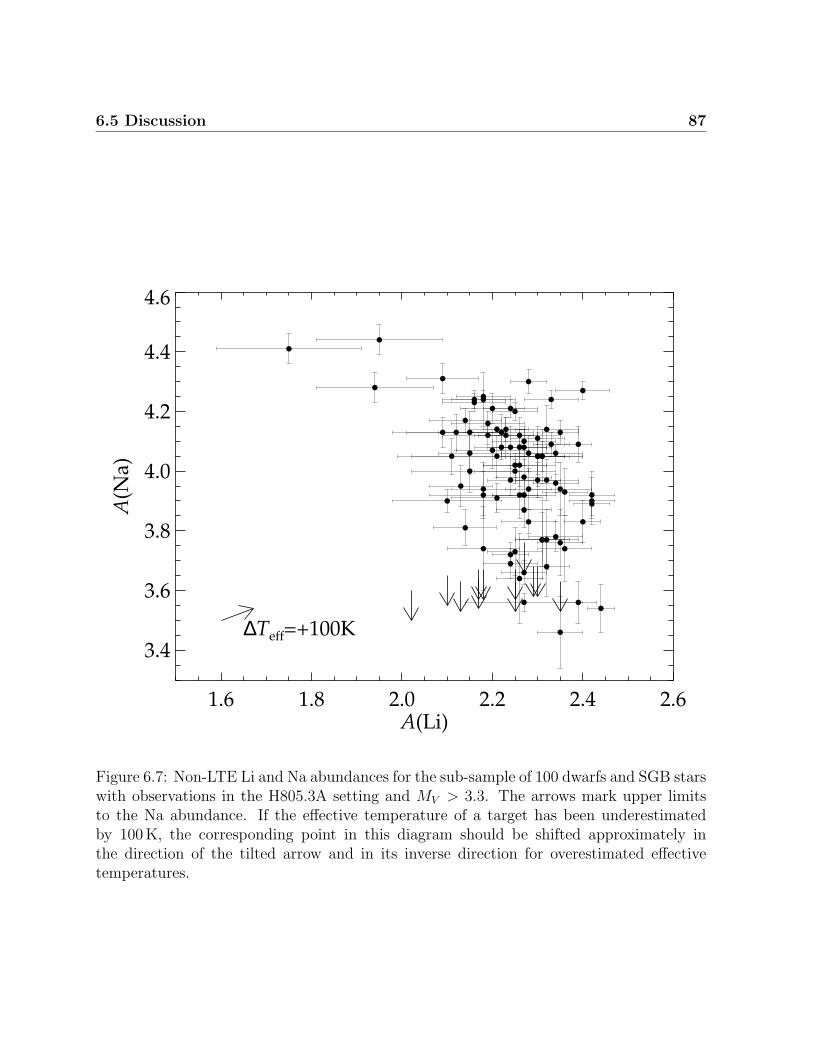
6.5 Discussion 87
1.6 1.8 2.0 2.2 2.4 2.6A(Li)
3.4
3.6
3.8
4.0
4.2
4.4
4.6
A(N
a)
∆Teff=+100K
Figure 6.7: Non-LTE Li and Na abundances for the sub-sample of 100 dwarfs and SGB starswith observations in the H805.3A setting and MV > 3.3. The arrows mark upper limitsto the Na abundance. If the effective temperature of a target has been underestimatedby 100K, the corresponding point in this diagram should be shifted approximately inthe direction of the tilted arrow and in its inverse direction for overestimated effectivetemperatures.
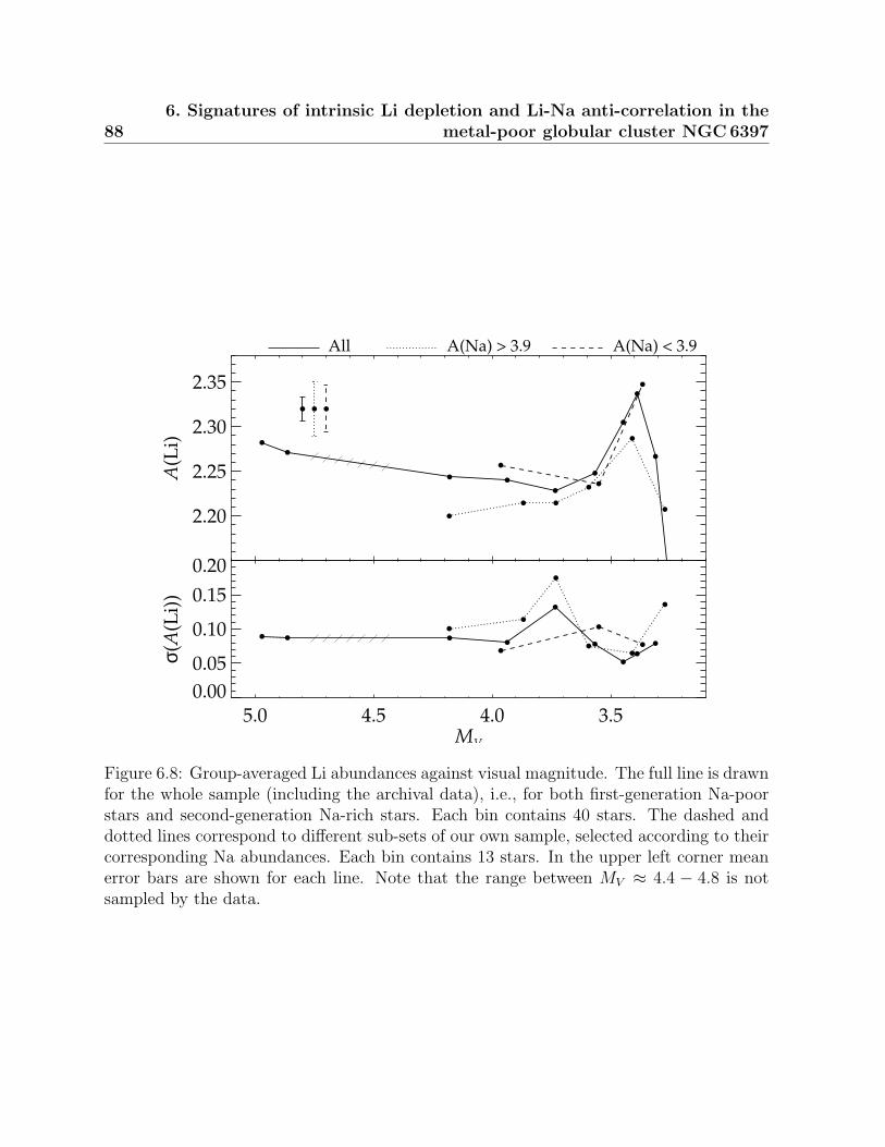
886. Signatures of intrinsic Li depletion and Li-Na anti-correlation in the
metal-poor globular cluster NGC 6397
2.20
2.25
2.30
2.35
A(L
i)
All A(Na) > 3.9 A(Na) < 3.9
5.0 4.5 4.0 3.5M
V
0.00
0.05
0.10
0.15
0.20
σ(A
(Li)
)
Figure 6.8: Group-averaged Li abundances against visual magnitude. The full line is drawnfor the whole sample (including the archival data), i.e., for both first-generation Na-poorstars and second-generation Na-rich stars. Each bin contains 40 stars. The dashed anddotted lines correspond to different sub-sets of our own sample, selected according to theircorresponding Na abundances. Each bin contains 13 stars. In the upper left corner meanerror bars are shown for each line. Note that the range between MV ≈ 4.4 − 4.8 is notsampled by the data.
6.5 Discussion 89
2.20
2.25
2.30
2.35
A(L
i)
All A(Na) > 3.9 A(Na) < 3.9
6500 6400 6300 6200 6100 6000 5900 5800Teff [K]
0.00
0.05
0.10
0.15
0.20
σ(A
(Li)
)
Figure 6.9: Group-averaged Li abundances against effective temperature. The lines corre-spond to the same sub-samples as in Fig. 6.8. Filled circles represent post-TO stars andopen squares pre-TO stars. In the upper left corner mean error bars are shown for eachline.
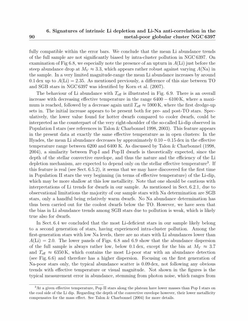
906. Signatures of intrinsic Li depletion and Li-Na anti-correlation in the
metal-poor globular cluster NGC 6397
fully compatible within the error bars. We conclude that the mean Li abundance trendsof the full sample are not significantly biased by intra-cluster pollution in NGC6397. Onexamination of Fig 6.8, we especially note the presence of an upturn in A(Li) just before thesteep abundance drop at MV ≈ 3.3, which appears rather robust against varying A(Na) inthe sample. In a very limited magnitude-range the mean Li abundance increases by around0.1 dex up to A(Li) = 2.35. As mentioned previously, a difference of this size between TOand SGB stars in NGC6397 was identified by Korn et al. (2007).
The behaviour of Li abundance with Teff is illustrated in Fig. 6.9. There is an overallincrease with decreasing effective temperature in the range 6400− 6100K, where a maxi-mum is reached, followed by a decrease again until Teff ≈ 5900K, where the first dredge-upsets in. The initial increase appears to be present both for pre- and post-TO stars. Spec-ulatively, the lower value found for hotter dwarfs compared to cooler dwarfs, could beinterpreted as the counterpart of the very right-shoulder of the so-called Li-dip observed inPopulation I stars (see references in Talon & Charbonnel 1998, 2003). This feature appearsin the present data at exactly the same effective temperature as in open clusters: In theHyades, the mean Li abundance decreases by approximately 0.10−0.15 dex in the effectivetemperature range between 6200 and 6400 K. As discussed by Talon & Charbonnel (1998,2004), a similarity between Pop I and Pop II dwarfs is theoretically expected, since thedepth of the stellar convective envelope, and thus the nature and the efficiency of the Lidepletion mechanism, are expected to depend only on the stellar effective temperature3. Ifthis feature is real (see Sect. 6.5.2), it seems that we may have discovered for the first timein Population II stars the very beginning (in terms of effective temperature) of the Li-dip,which may be more shallow at this low metallicity. Note that one should be cautious withinterpretations of Li trends for dwarfs in our sample. As mentioned in Sect. 6.2.1, due toobservational limitations the majority of our sample stars with Na determination are SGBstars, only a handful being relatively warm dwarfs. No Na abundance determination hasthus been carried out for the coolest dwarfs below the TO. However, we have seen thatthe bias in Li abundance trends among SGB stars due to pollution is weak, which is likelytrue also for dwarfs.
In Sect. 6.4 we concluded that the most Li-deficient stars in our sample likely belongto a second generation of stars, having experienced intra-cluster pollution. Among thefirst-generation stars with low Na levels, there are no stars with Li abundances lower thanA(Li) = 2.0. The lower panels of Figs. 6.8 and 6.9 show that the abundance dispersionof the full sample is always rather low, below 0.1 dex, except for the bin at MV ≈ 3.7and Teff ≈ 6350K, which contains the most Li-poor star with an abundance detection(see Fig. 6.6) and therefore has a higher dispersion. Focusing on the first generation ofNa-poor stars only, the typical abundance scatter is 0.09 dex, not following any obvioustrends with effective temperature or visual magnitude. Not shown in the figures is thetypical measurement error in abundance, stemming from photon noise, which ranges from
3At a given effective temperature, Pop II stars along the plateau have lower masses than Pop I stars onthe cool side of the Li dip. Regarding the depth of the convective envelope however, their lower metallicitycompensates for the mass effect. See Talon & Charbonnel (2004) for more details.
6.5 Discussion 91
0.08 dex for the hottest stars to 0.05 dex for the coolest plateau stars. To this measurementerror should be added the propagated uncertainty in stellar parameters. Assuming that thetypical star-to-star error in effective temperature, which is the most influential parameter,lies in the range 50 − 100K, a corresponding additional spread of 0.04 − 0.07 dex in Liabundance is expected. Given these basic estimates, we conclude that the observations arecompatible with zero scatter in Li abundance among the first-generation stars.
6.5.2 Effects of stellar parameters and non-LTE
We now briefly discuss the influence on the abundance trends presented in Sect. 6.5.1 fromthe choice of effective-temperature scale and from the non-LTE treatment. Basically, botheffects have a systematic influence over the Li data. If we were to adopt the IRFM-basedeffective-temperature scale by Ramırez & Melendez (2005) (see Sect. 6.3.1) the Li abun-dances of post-TO stars would be systematically lowered by −0.06 dex, thus aggravatingfurther the overall discrepancy to the primordial value. The scale by Alonso et al. (1996,1999) would act in the same direction, but also have a minor differential impact on theLi abundances since this effective-temperature scale is steeper in the range from the TOto further up the SGB. The TO star abundances would therefore be lowered by a greateramount (−0.1 dex) than the cooler SGB star abundances, which in turn would enhancethe abundance upturn seen in Fig. 6.8 and the corresponding maximum abundance seenin Fig. 6.9 at Teff = 6100K. Nothing would thus qualitatively change in the discussionof abundance trends for post-TO stars. However, implementing either of the two IRFM-based scales would lower the abundances found for cool dwarfs more than hot dwarfs. Thedifference between these two groups discussed in Sect. 6.5.1, which we speculated could bea signature of the Li-dip, would hence be erased.
As mentioned in Sect. 6.3.3, the non-LTE abundance corrections are similar, approx-imately −0.06 dex, for all plateau stars. The LTE abundances therefore have the samerelative behaviour but are offset to a slightly higher values.
6.5.3 Comparison to other studies
Comparing the found Li abundances to other determinations made for NGC6397, we findgood agreement with Korn et al. (2007), who place their five TO stars with MV ≈ 3.6at A(Li) = 2.25 and two SGB stars with MV ≈ 3.3 at A(Li) = 2.36. The similaritybetween the abundances for TO and SGB stars is partly due to the cancellation betweenthe effects from the cooler effective-temperature scale of Korn et al. (2007) and the fact thatthey do not correct for non-LTE. For RGB stars the two effects do not cancel (non-LTEcorrections are positive for RGB stars) and Korn et al. (2007) thus find abundances thatare approximately 0.1 dex lower than ours. The Li abundances reported by Bonifacio et al.(2002) for TO stars lie on average 0.1 dex higher than ours. This difference can be fullytraced to their effective-temperature scale, which is hotter by approximately 50K than theone adopted in this study, and to their use of different non-LTE corrections (Carlsson et al.,1994). For these stars, the corrections by Carlsson et al. (1994) are smaller in absolute
926. Signatures of intrinsic Li depletion and Li-Na anti-correlation in the
metal-poor globular cluster NGC 6397
value than the ones found by Lind et al. (2009a). The Li abundances and abundance upperlimits reported by Castilho et al. (2000) for 16 RGB stars are in good agreement with ours,except for the Li detections made for giants cooler than 4900K, which are significantlyhigher than what we find.
In the extensive literature study of field stars carried out by Charbonnel & Primas(2005), the authors concluded that the stars in their TO and SGB samples generally aremore Li-rich than their dwarf sample. Especially, dwarfs that are cooler than 6000K showa distinct decrease in Li abundance with decreasing effective temperature. As the dwarfsin our sample are all hotter than 6000K we cannot verify this result. However, withhindsight one may trace a tendency of increasing Li abundance with decreasing effectivetemperature in the range Teff = 6050 − 6400K among the MS, TO, and post-TO starsobserved by Charbonnel & Primas (2005) (see their online tables 5-9), similar to the onewe find.
6.5.4 Comparison to diffusion-turbulence models
Fig. 6.10 and Fig. 6.11 show comparisons of our obtained Li abundances with the pre-dictions from stellar-structure models including atomic diffusion from first principles andan ad-hoc recipe for turbulent mixing (Richard et al. 2005 and references therein). Forclarity we show the same group-averaged Li abundances as in Fig. 6.8 and Fig. 6.9, in-cluding the whole sample, irrespectively of Na abundance. Only post-TO stars appear inFig. 6.11. For comparison, the bottom panels of both figures show corresponding trendsfor binned Ca abundances. Visual magnitudes are converted to stellar luminosities usingthe bolometric corrections of Alonso et al. (1999). The same three models, T5.80, T6.00,and T6.09, with different efficiencies of turbulent transport, as displayed in Korn et al.(2007); Lind et al. (2008) are shown. To ensure that the model Teff − log(L/L)-planeis in agreement with our study regarding the location of the TO-point, we add +80K tothe effective-temperature scale of Richard et al. (2005) and +0.05 dex to the logarithmicluminosity-scale. The absolute abundance scale of the models is shifted to agree with theobservations for stars evolved beyond the onset of the first dredge-up.
The efficiency of turbulent mixing determines how much Li that is transported betweenthe external convection zone to the region in the stellar interior where Li is destroyed, whichin turn has influences over the appearance of the Li abundance plateau. In the T6.09 model,with highest efficiency, the plateau is flat, whereas the surface abundances predicted by theT5.80 model show a clear dependence on stellar luminosity and effective temperature. Asseen in Fig. 6.10, the Li abundances of NGC 6397 strictly limit the efficiency of turbulentmixing, although no model perfectly reproduces the observed abundances. In terms of thesize of the Li variations on the plateau, the T6.00 model appears to be the best choice, sup-porting the findings by Korn et al. (2007); Lind et al. (2008). The observed Ca abundancetrend is in good agreement with both higher-efficiency models (T6.00 and T6.09), andespecially the location of the upturn at log(L/L) ≈ 0.65 is matched. However, Fig. 6.11shows clearly that the behaviour of the post-TO Li abundance with effective temperatureis not reproduced by any of the models. Especially the location of the maximum A(Li)
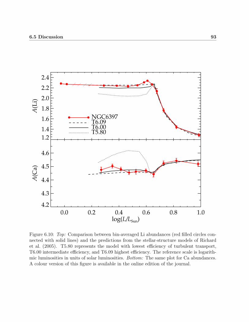
6.5 Discussion 93
1.2
1.4
1.6
1.8
2.0
2.2
2.4
A(L
i)
NGC6397T6.09T6.00T5.80
0.0 0.2 0.4 0.6 0.8 1.0log(L/LSun)
4.2
4.3
4.4
4.5
4.6
A(C
a)
Figure 6.10: Top: Comparison between bin-averaged Li abundances (red filled circles con-nected with solid lines) and the predictions from the stellar-structure models of Richardet al. (2005). T5.80 represents the model with lowest efficiency of turbulent transport,T6.00 intermediate efficiency, and T6.09 highest efficiency. The reference scale is logarith-mic luminosities in units of solar luminosities. Bottom: The same plot for Ca abundances.A colour version of this figure is available in the online edition of the journal.
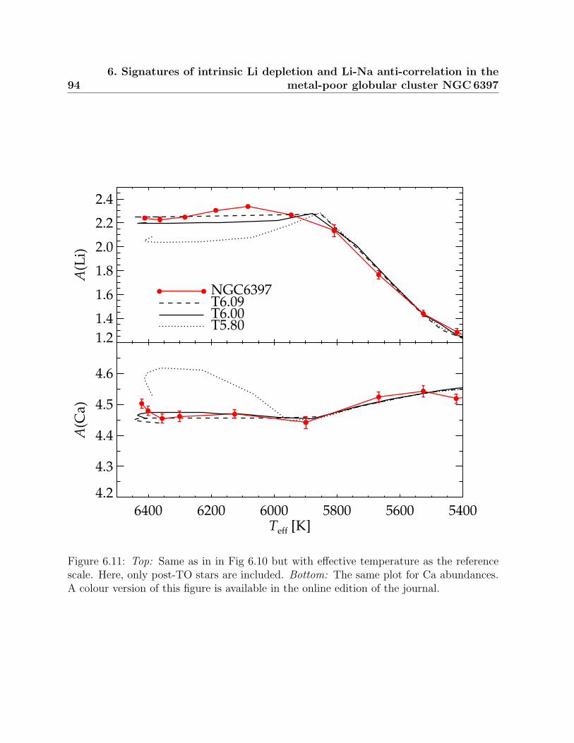
946. Signatures of intrinsic Li depletion and Li-Na anti-correlation in the
metal-poor globular cluster NGC 6397
1.2
1.4
1.6
1.8
2.0
2.2
2.4
A(L
i)
NGC6397T6.09T6.00T5.80
6400 6200 6000 5800 5600 5400Teff [K]
4.2
4.3
4.4
4.5
4.6
A(C
a)
Figure 6.11: Top: Same as in in Fig 6.10 but with effective temperature as the referencescale. Here, only post-TO stars are included. Bottom: The same plot for Ca abundances.A colour version of this figure is available in the online edition of the journal.
6.6 Conclusions 95
occurs at higher effective temperature than the models predict.The initial Li abundance predicted by the models, accounting for the adjustment we
make in the vertical direction, is A(Li) = 2.46, which is significantly closer, but still not infull agreement with the latest predictions from BBNS of 2.72± 0.06 (Cyburt et al., 2008).
6.6 Conclusions
We have presented a comprehensive study of the Li content in a large sample, 454 starsin total, of MS, TO, SGB, and RGB stars in the metal-poor globular cluster NGC6397.The cluster dwarfs and early SGB stars form a thin Li abundance plateau on the samelevel as the Spite plateau for field stars, whereas more evolved stars have undergone dras-tic Li depletion due to physical processes connected to low-mass stellar evolution. Tworemarkably well-defined locations in absolute visual magnitudes, MV ≈ 3.3 and MV ≈ 0.0respectively, are identified as the locations of corresponding steep Li abundance drops.They correspond respectively to the occurrence of the first dredge-up on the SGB and tothe onset of thermohaline mixing at the RGB bump (Charbonnel & Zahn, 2007).
Using information of Li and Na abundance for a sub-sample of 100 dwarfs and earlySGB, we have for the first time identified a significant anti-correlation between the twoelements in this cluster. This is interpreted as the signature of intra-cluster pollution froma previous generation of more massive stars. The spread in Na and Li abundances of starsnot having undergone Li depletion due to dredge-up, is very large, about one order-of-magnitude. However, only a handful of stars show significantly depleted Li levels and theidentified anti-correlation depends critically on these objects. For Na-enhancements up to0.7 dex, no corresponding Li-deficiency can be detected. The average Li abundance is thusnot much affected by internal pollution. These abundance patterns have consequences forfor the self-enrichment scenario in NGC6397, which will be discussed in a forth-comingpaper.
By dividing our sub-sample with Na determinations into two groups, consisting offirst and second generation of stars according to the degree of pollution, we illustratehow especially trends of Li abundance with effective temperature and evolutionary phaseare in reasonable agreement between the two generations. The average Li abundance istypically A(Li) = 2.25 for stars located below and above the TO, and show a slight upturnof ∆A(Li) ≈0.1 dex for stars in the middle of the SGB. This difference agrees with withprevious findings for the cluster as well as for field stars. We find no support for a significantLi dispersion among the first generation of stars.
The identification of a minor Li deficiency of the hottest dwarfs in our sample comparedto slightly cooler dwarfs leads us to suggest that the very right-hand wing of the Li-dipmay be visible also among Pop II stars. However, the signature is erased if a differenteffective temperature scale is adopted.
The detailed picture we have formed of the Li abundance trends in this globular clustercan be used to constrain the physics involved in depleting Li from the photospheres oflow-mass metal-poor stars, as well as the extent of the depletion. To illustrate this, we
966. Signatures of intrinsic Li depletion and Li-Na anti-correlation in the
metal-poor globular cluster NGC 6397
compare our observational findings to predictions from stellar-structure models includingatomic diffusion, with additional turbulence below the convection zone. We find that someturbulence, in a very limited efficiency-range, is indeed required to explain observations.However, these models fail to reproduce the behaviour of Li abundance with effectivetemperature along the plateau, suggesting that a detailed understanding of the physicsresponsible for depletion is still lacking.
Chapter 7
Tracing the evolution of NGC 6397through the chemical composition ofits stellar populations
The following article has been recommended for publication in Astronomy & Astrophysicsin August 2010 (Lind, Charbonnel, Decressin, Primas, Grundahl, & Asplund). The workhas been based on data collected at European Southern Observatory (ESO), Paranal, Chile,under program IDs 077.A-0018(A) and 281.D-5028(A), as well as data collected with theDanish 1.54m telescope at European Southern Observatory (ESO), La Silla.
7.1 Introduction
The abundance patterns of light elements (up to Al) in globular clusters are being carefullyinvestigated. Especially, the origin of the larger spread in C, N, O, Na, Mg, and Alabundances compared to field stars of similar metallicity is being traced. The present statusof the observed light element (O, Na, Mg, and Al) abundances in globular clusters andpossible consequences for the formation and enrichment history of these stellar populations,have been mapped in a recent series of publications by (e.g. Carretta et al. 2009a, 2010),see also reviews by Gratton et al. (2004) and Charbonnel (2005). The main findings, asinferred from high-resolution spectroscopy of individual globular cluster stars, are apparentenhancements of N, Na, and Al abundances and deficiencies in Li, O, and Mg. Suchpatterns can be naturally explained by enrichment of the nucleosynthesis rest-products ofH-burning at high temperatures (Denisenkov & Denisenkova, 1989; Langer et al., 1993).Since the resulting anti-correlations between particularly O–Na abundances have not onlybeen seen in evolved RGB stars, but also in TO and SGB stars (Gratton et al., 2001), anintrinsic stellar evolutionary cause is very unlikely, i.e. the stars can not have establishedthese abundance patterns themselves. Rather, it is believed that the gas that formedsecond generation stars in globular clusters underwent early pollution by slow ejecta fromintermediate mass or massive stars.
987. Tracing the evolution of NGC 6397 through the chemical composition of its
stellar populations
Important in this context is also photometric evidence of multiplicity in some clusters,like ω Cen and NGC2808, in which several parallel main sequences can be identified. Theseobservations seemingly necessitate that a difference in the He content is present (e.g. Norris2004), in qualitative agreement with the self-enrichment process responsible for the otherlight element variations. He enrichment is also commonly invoked to explain the extendedhorizontal branch observed in many clusters (D’Antona & Caloi, 2008). We are, however,far from building a fully consistent picture of the chemical evolution of globular clustersthat can explain all the various observations simultaneously.
A key issue that remains to be settled is the properties of the polluting objects. Onepossibility is that so called hot bottom burning occurs at the base of the convective envelopein intermediate-mass stars during the asymptotic giant branch (AGB) phase, which wouldleave nucleosynthesis products in the envelope that is subsequently expelled (Ventura &D’Antona, 2008, 2010). Also, super-AGB stars have been suggested to be responsible forthe most extreme anomalies (Pumo et al., 2008). The main alternative scenario is a slowmechanical wind from rapidly rotating massive stars (e.g. Decressin et al. 2007a), whoseenvelopes have been enriched in H-burning products by deep internal mixing (see Sect. 7.4).Yet another option is mass loss from massive binary systems, as suggested by de Mink et al.(2009).
By accurate abundance analysis of many elements (and isotopic ratios) in large stellarsamples, we may pin-point the nature of the progenitors (e.g. Charbonnel 2005, andreferences therein). A common property of the competing scenarios is that the pollutionwould alter mainly the light element abundances of second generation stars in globularclusters, thus leaving α and iron-peak elements unaffected. This is necessary to explainthe homogeneous composition of these elements seen in most clusters. Elements createdin the s-process may be affected by AGB pollution, suggesting the presence of correlationsbetween s-process and light element anomalies. In NGC6752, an unexplained correlationwas indeed identified between Al abundances and Y, Zr, and Ba (Yong et al., 2005), but thesystematic heavy elements variations are small (0.1 dex) and comparable to the statisticalscatter. One must also bear in mind that the yields of AGB stars are uncertain (e.g.Charbonnel 2007; Decressin et al. 2009; Ventura & D’Antona 2010).
In addition to mapping the presence of abundance trends and correlations it is alsoessential to investigate, preferably with sound number statistics, the fraction of stars withnormal chemical composition, similar to the field, and the fraction of second and possi-bly third generation stars in globular clusters. Linking this information to other clusterobservables one may construct a schematic model for the episodes of star formation andevolution. Carretta et al. (2010) describe a possible general formation scenario in whicha precursor population, forming from the gas assembled at a very early epoch inside aCDM halo, efficiently raises the metal content of the gas cloud via core-collapse supernovaexplosions. Those trigger a second, large episode of star formation, the so called primor-dial population (first generation). The slow winds of massive or intermediate-mass stars ofthe primordial population feed a cooling flow, and the intermediate (second) generation ofstars are formed in the central parts of the cluster, out of material enriched in H-burningproducts. The remaining gas is dispersed by core-collapse supernovae of the second gen-

7.2 Observations and analysis 99
eration and star formation ceases. The present-day cluster is dominated by the secondgeneration, with a smaller fraction, approximately 30%, left of the primordial population.Critical factors that determine the outcome of such a scenario is the initial mass function(IMF) of the polluting stars, the initial total mass of the cluster, and the amount of mixingbetween processed gas in the slow stellar ejecta and pristine cluster gas. We will discussthese issues further in Sect. 7.4.
HST photometry of NGC6397 produces a remarkably clean HR-diagram, with a verytight MS (Richer et al., 2008) and a very compact blue horizontal branch, i.e. there are noobvious photometric signs of multiple populations. The cluster is well-studied in terms ofnumber of stars for which high-resolution spectra have been obtained, but only a handfulof elements have previously been analysed even on the RGB (most recently by Grattonet al. 2000; Castilho et al. 2000; Thevenin et al. 2001; Korn et al. 2007; Carretta et al.2009a), as summarised in Table 7.1.
Early studies of the strengths of the G and CN band in RGB stars in NGC6397 (andother clusters) suggested anomalies in C and N abundance (Bell et al., 1979; Briley et al.,1990). Eventually, Gratton et al. (2001) also detected a significant spread in Na abundancefor a sample of ten TO stars and RGB stars, findings that clearly pointed to an intrinsic,rather than evolutionary, origin. Later, Carretta et al. (2005) corroborated these findingsfor a larger sample of stars and also found a significant O–Na anti-correlation, as wellas a large spread in C and N abundance (see also Pasquini et al. 2004). In the latestanalysis by Carretta et al. (2009b,a) the O–Na anti-correlation is present, although thenumber statistics are still rather small, especially oxygen measurements are few. A Mg–Al anti-correlation has not been identified in NGC 6397, but Mg also seems to show acertain scatter (Korn et al., 2007). Lind et al. (2009b) presented Na abundances for > 100TO, SGB, and RGB stars, and found that the most heavily Na-enriched stars also aresignificantly depleted in Li. It is thus clear that NGC6397, like other globular clusters,should no longer be regarded as a single stellar population despite the tightness of itscolour-magnitude diagram. However, even if pollution indeed seems to have taken place inthe cluster, it is unclear to which extent, and which elements are affected by it. With thisstudy, targeting red giants, we will cover as many elements as possible, for a large sampleof stars and give a more decisive answer to this question.
7.2 Observations and analysis
We have obtained high-resolution (R = 47000) spectra with the multi-object fibre spec-trograph FLAMES/UVES on the VLT, covering the wavelength range 480–680 nm (UVESRed 580 standard setting). For a subset of six stars, we also have spectra covering thewavelength range 760–1000 nm (UVES Red 860 standard setting). Our targets are allRGB stars, whose surface abundances should reflect the initial composition of cluster gas,with the notable exceptions of Li and Be, which are not studied here (Li abundances werepublished in Lind et al. 2009b). In particular, any internal abundance gradients createdby atomic diffusion (Korn et al., 2007; Lind et al., 2008) during the time on the MS have
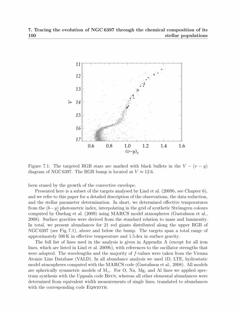
1007. Tracing the evolution of NGC 6397 through the chemical composition of its
stellar populations
0.6 0.8 1.0 1.2 1.4 1.6
(v−y)0
17
16
15
14
13
12
11V
Figure 7.1: The targeted RGB stars are marked with black bullets in the V − (v − y)diagram of NGC 6397. The RGB bump is located at V ≈ 12.6.
been erased by the growth of the convective envelope.Presented here is a subset of the targets analysed by Lind et al. (2009b, see Chapter 6),
and we refer to this paper for a detailed description of the observations, the data reduction,and the stellar parameter determination. In short, we determined effective temperaturesfrom the (b−y) photometric index, interpolating in the grid of synthetic Stromgren colourscomputed by Onehag et al. (2009) using MARCS model atmospheres (Gustafsson et al.,2008). Surface gravities were derived from the standard relation to mass and luminosity.In total, we present abundances for 21 red giants distributed along the upper RGB ofNGC 6397 (see Fig. 7.1), above and below the bump. The targets span a total range ofapproximately 500K in effective temperature and 1.5 dex in surface gravity.
The full list of lines used in the analysis is given in Appendix A (except for all ironlines, which are listed in Lind et al. 2009b), with references to the oscillator strengths thatwere adopted. The wavelengths and the majority of f -values were taken from the ViennaAtomic Line Database (VALD). In all abundance analysis we used 1D, LTE, hydrostaticmodel atmospheres computed with the MARCS code (Gustafsson et al., 2008). All modelsare spherically symmetric models of M. For O, Na, Mg, and Al lines we applied spec-trum synthesis with the Uppsala code Bsyn, whereas all other elemental abundances weredetermined from equivalent width measurements of single lines, translated to abundanceswith the corresponding code Eqwidth.

7.3 Abundance analysis 101
Abundance ratios with respect to the Sun were calculated using the solar abundancesof Asplund et al. (2009). We stress that our main concern is the relative abundance scalewithin the cluster, rather than absolute abundances. With our fully homogeneous analysiswe constrain relative stellar parameters and abundances very well. The listed abundanceerrors reflect only on the measurement uncertainty, as estimated from the signal-to-noiseratio of the spectra (Norris et al., 2001), and do not consider uncertainties in the adoptedstellar parameters. Upper limits to the equivalent width, and hence the abundance, arecalculated by adding twice the estimated measurement uncertainty to the best fittingsynthetic spectra.
Fig. 7.2 shows the observed and best-fit model spectra of O, Na, Mg, and Al lines intwo RGB stars, #17691 and #12138. The abundances of these four elements are all basedon weak lines, whose line formation do not depart substantially from LTE. For Na only,we compute and adopt non-LTE abundances for all targets, whereas LTE is assumed tohold for the other species. The oxygen abundance is determined from the forbidden line at630 nm, which is believed to have negligible non-LTE corrections, but may be sensitive togranulation effects (Kiselman, 2001; Nissen et al., 2002). For the four targets for which thiswas possible, we have also determined the oxygen abundance based on the near infra-redtriplet lines at 777.1 nm and 777.4 nm, with very good agreement with the 630 nm linein LTE. Fabbian et al. (2009) predict non-LTE corrections for the triplet lines to be oforder (−0.05) − (−0.08) dex for our targets, adopting hydrogen collisions with SH = 1.0(Pereira et al., 2009a). Applying this correction would slightly lessen the agreement withthe forbidden line.
The Na abundances are based on the 568.2 nm and 568.8 nm lines, which have non-LTE corrections ≈ −0.07 dex for stars with these stellar parameters (Lind et al. submit-teda, see Chapter 2). For five targets we have compared the abundances inferred fromthe 568.2/568.8 nm lines with those inferred from the 818.3/819.4 nm lines by Lind et al.(2009b). As seen in Fig. 7.4, the non-LTE corrected abundances agree well within theuncertainties. The Mg abundance is determined from the Mg line at 571.1 nm, for whichShimanskaya et al. (2000) report non-LTE corrections that are smaller than 0.02 dex forthe relevant stellar parameters. The doublet lines of neutral Al at 669.6/669.8 nm are usedto infer the Al abundance. We have not found any non-LTE calculations in the literaturefor these lines in metal-poor giant stars, but since they are weak, high-excitation lines, theyshould at least be more reliable abundance indicators in LTE than the stronger ultra-violetresonance lines at 396.1/394.4 nm (e.g. Asplund 2005). Furthermore, since our targets allhave quite similar stellar parameters the differential non-LTE effects should be small.
7.3 Abundance analysis
Fig. 7.3 shows [Fe/H] and abundance ratios relative to Fe 1 for all stars. Table 7.1 liststhe mean abundance and dispersion of all elements, compared to values found in the
1[X/Y ] = log(
N(X)N(Y )
)∗− log
(N(X)N(Y )
)
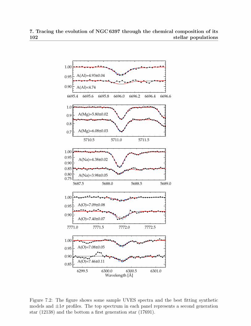
1027. Tracing the evolution of NGC 6397 through the chemical composition of its
stellar populations
6299.5 6300.0 6300.5 6301.0Wavelength [Å]
0.85
0.90
0.95
1.00
A(O)=7.46±0.11
A(O)=7.08±0.05
7771.0 7771.5 7772.0 7772.5
0.90
0.95
1.00
A(O)=7.40±0.07
A(O)=7.09±0.08
5687.5 5688.0 5688.5 5689.00.750.800.850.900.951.00
A(Na)=3.98±0.05
A(Na)=4.38±0.02
5710.5 5711.0 5711.5
0.7
0.8
0.9
1.0
A(Mg)=6.08±0.03
A(Mg)=5.80±0.02
6695.4 6695.6 6695.8 6696.0 6696.2 6696.4 6696.6
0.90
0.95
1.00
A(Al)<4.74
A(Al)=4.93±0.04
Figure 7.2: The figure shows some sample UVES spectra and the best fitting syntheticmodels and ±1σ profiles. The top spectrum in each panel represents a second generationstar (12138) and the bottom a first generation star (17691).

7.3 Abundance analysis 103
+0.0
0.2
0.4
0.6
0.8
[O/
Fe]
−0.4
−0.2
0.0
0.2
0.4
[Na/
Fe]
−0.2
0.0
0.2
0.4
0.6
[Mg
/F
e]
+0.0
0.2
0.4
0.60.8
[Al/
Fe]
−0.2
0.0
0.2
0.4
0.6
[Si/
Fe]
−0.2
0.0
0.2
0.4
0.6
[Ca/
Fe]
5300 5200 5100 5000 4900 4800 4700Teff
−0.4
−0.2
0.0
0.2
0.4
[Sc/
Fe]
−0.2
0.0
0.2
0.4
0.6[T
i/F
e]
−0.4
−0.2
0.0
0.20.4
[Cr/
Fe]
−1.0
−0.8
−0.6
−0.4
−0.2
[Mn
/F
e]
−2.6
−2.4
−2.2
−2.0
−1.8
[Fe/
H]
−0.4
−0.2
0.0
0.2
0.4
[Co
/F
e]
−0.6
−0.4
−0.2
0.0
0.2
[Ni/
Fe]
5300 5200 5100 5000 4900 4800 4700Teff
−1.4
−1.2
−1.0
−0.8
−0.6
[Cu
/F
e]
−0.4
−0.2
0.0
0.20.4
[Zn
/F
e]
−0.8
−0.6
−0.4
−0.2
0.0
[Y/
Fe]
−0.4
−0.2
0.0
0.2
0.4
[Zr/
Fe]
−0.6
−0.4
−0.2
0.0
0.2
[Ba/
Fe]
+0.0
0.2
0.4
0.60.8
[Ce/
Fe]
−0.2
0.0
0.2
0.4
[Nd
/F
e]
5300 5200 5100 5000 4900 4800 4700Teff
+0.0
0.2
0.4
0.60.8
[Eu
/F
e]
Figure 7.3: Elemental abundances of all targets. Each panel spans 1 dex in abundance andmarks the average abundance (solid line) and the 1σ dispersion limits (dashed lines). Twodifferent symbols are used for [Ti/Fe], [Cr/Fe], and [Fe/H]: the red open bullets and theblack filled bullets in these panels represent abundances inferred from neutral and singlyionised lines, respectively. The hottest star in each panel mark the completeness limit, i.e.all sample stars cooler than this limit are shown.
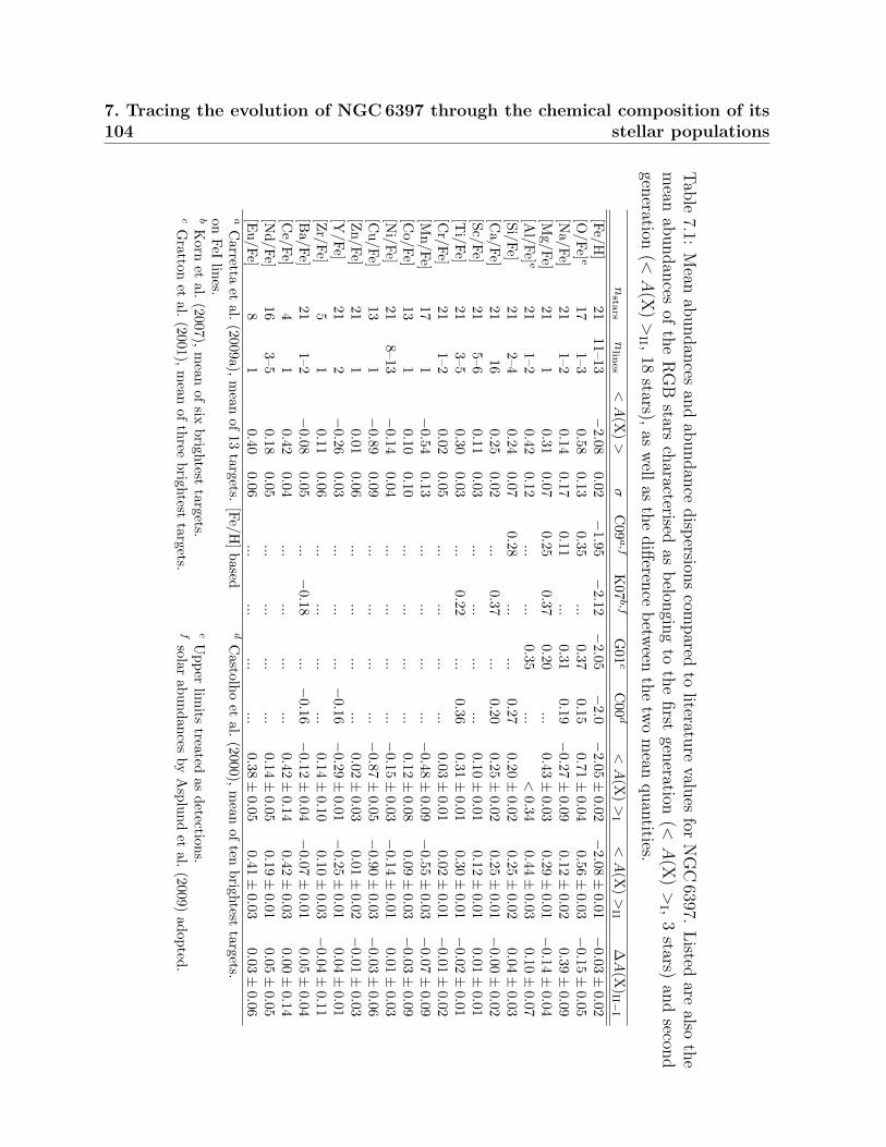
1047. Tracing the evolution of NGC 6397 through the chemical composition of its
stellar populations
Tab
le7.1:
Mean
abundan
cesan
dab
undan
cedisp
ersions
compared
toliteratu
revalu
esfor
NG
C6397.
Listed
arealso
the
mean
abundan
cesof
the
RG
Bstars
characterised
asbelon
ging
toth
efirst
generation
(<A
(X)
>I ,
3stars)
and
second
generation
(<A
(X)>
II ,18
stars),as
well
asth
ediff
erence
betw
eenth
etw
om
eanquan
tities.
nsta
rsn
lines
<A
(X)
>σ
C09
a,f
K07
b,f
G01
cC
00d
<A
(X)
>I
<A
(X)
>II
∆A
(X)II−
I
[Fe/H]
2111–13
−2.08
0.02
−1.95
−2.12
−2.05
−2.0−
2.05±
0.02−
2.08±
0.01−
0.03±
0.02[O
/Fe] e17
1–30.58
0.13
0.35
...0.37
0.150.71±
0.04
0.56±
0.03
−0.15
±0.05
[Na/Fe]
211–2
0.140.17
0.11
...0.31
0.19−
0.27±
0.090.12±
0.02
0.39±
0.09
[Mg/Fe]
211
0.310.07
0.25
0.370.20
...0.43
±0.03
0.29±
0.01−
0.14±
0.04[A
l/Fe] e21
1–20.42
0.12
......
0.35
...<
0.34
0.44±
0.03
0.10±
0.07[Si/Fe]
212–4
0.24
0.07
0.28
......
0.27
0.20±
0.02
0.25±
0.02
0.04±
0.03[C
a/Fe]
2116
0.25
0.02
...0.37
...0.20
0.25±
0.020.25±
0.01−
0.00±
0.02[Sc/Fe]
215–6
0.110.03
......
......
0.10±
0.010.12±
0.010.01±
0.01
[Ti/Fe]
213–5
0.300.03
...0.22
...0.36
0.31±
0.010.30±
0.01−
0.02±
0.01[C
r/Fe]21
1–20.02
0.05
......
......
0.03±
0.010.02±
0.01−
0.01±
0.02[M
n/Fe]
171
−0.54
0.13
......
......
−0.48±
0.09−
0.55±
0.03−
0.07±
0.09[C
o/Fe]
131
0.10
0.10
......
......
0.12±
0.080.09±
0.03−
0.03±
0.09[N
i/Fe]21
8–13−
0.140.04
......
......
−0.15±
0.03−
0.14±
0.010.01±
0.03
[Cu/Fe]
131
−0.89
0.09
......
......
−0.87±
0.05
−0.90
±0.03
−0.03
±0.06
[Zn/Fe]
211
0.010.06
......
......
0.02±
0.030.01±
0.02−
0.01±
0.03[Y
/Fe]21
2−
0.260.03
......
...−
0.16
−0.29
±0.01
−0.25
±0.01
0.04±
0.01[Z
r/Fe]5
10.11
0.06
......
......
0.14±
0.100.10±
0.03−
0.04±
0.11[B
a/Fe]
211–2
−0.08
0.05
...−
0.18
...−
0.16
−0.12
±0.04
−0.07
±0.01
0.05±
0.04[C
e/Fe]4
10.42
0.04
......
......
0.42±
0.140.42±
0.030.00±
0.14
[Nd/Fe]
163–5
0.180.05
......
......
0.14±
0.050.19±
0.01
0.05±
0.05
[Eu/Fe]
81
0.40
0.06
......
......
0.38±
0.050.41±
0.03
0.03±
0.06
aC
arrettaet
al.(2009a),mean
of13
targets.[Fe/H
]basedon
FeIlines.
dC
astolhoet
al.(2000),
mean
often
brightesttargets.
bK
ornet
al.(2007),
mean
ofsix
brightesttargets.
eU
pperlim
itstreated
asdetections.
cG
rattonet
al.(2001),
mean
ofthree
brightesttargets.
fsolar
abundancesby
Asplund
etal.
(2009)adopted.
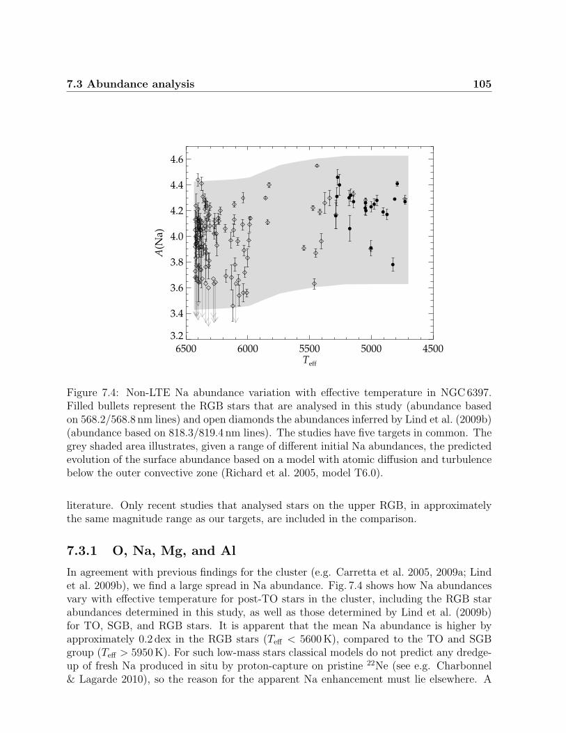
7.3 Abundance analysis 105
6500 6000 5500 5000 4500Teff
3.2
3.4
3.6
3.8
4.0
4.2
4.4
4.6A(N
a)
Figure 7.4: Non-LTE Na abundance variation with effective temperature in NGC6397.Filled bullets represent the RGB stars that are analysed in this study (abundance basedon 568.2/568.8 nm lines) and open diamonds the abundances inferred by Lind et al. (2009b)(abundance based on 818.3/819.4 nm lines). The studies have five targets in common. Thegrey shaded area illustrates, given a range of different initial Na abundances, the predictedevolution of the surface abundance based on a model with atomic diffusion and turbulencebelow the outer convective zone (Richard et al. 2005, model T6.0).
literature. Only recent studies that analysed stars on the upper RGB, in approximatelythe same magnitude range as our targets, are included in the comparison.
7.3.1 O, Na, Mg, and Al
In agreement with previous findings for the cluster (e.g. Carretta et al. 2005, 2009a; Lindet al. 2009b), we find a large spread in Na abundance. Fig. 7.4 shows how Na abundancesvary with effective temperature for post-TO stars in the cluster, including the RGB starabundances determined in this study, as well as those determined by Lind et al. (2009b)for TO, SGB, and RGB stars. It is apparent that the mean Na abundance is higher byapproximately 0.2 dex in the RGB stars (Teff < 5600K), compared to the TO and SGBgroup (Teff > 5950K). For such low-mass stars classical models do not predict any dredge-up of fresh Na produced in situ by proton-capture on pristine 22Ne (see e.g. Charbonnel& Lagarde 2010), so the reason for the apparent Na enhancement must lie elsewhere. A
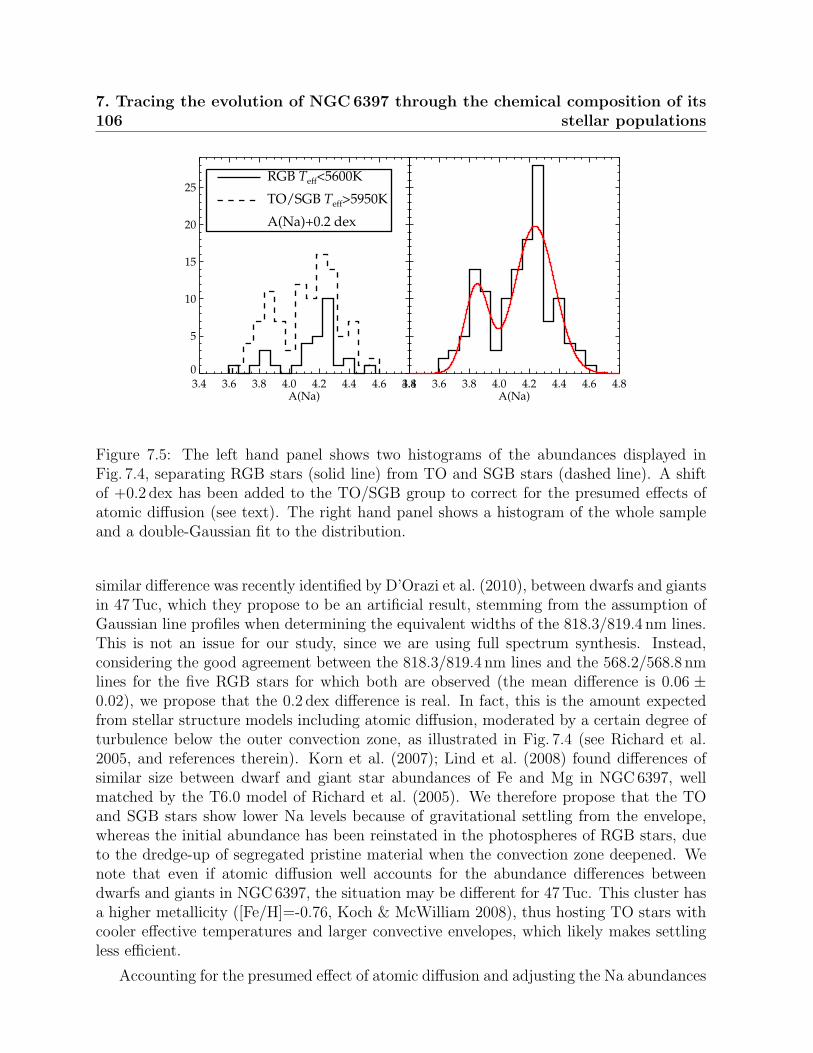
1067. Tracing the evolution of NGC 6397 through the chemical composition of its
stellar populations
3.4 3.6 3.8 4.0 4.2 4.4 4.6 4.8A(Na)
0
5
10
15
20
25RGB Teff<5600K TO/SGB Teff>5950K A(Na)+0.2 dex
3.4 3.6 3.8 4.0 4.2 4.4 4.6 4.8A(Na)
Figure 7.5: The left hand panel shows two histograms of the abundances displayed inFig. 7.4, separating RGB stars (solid line) from TO and SGB stars (dashed line). A shiftof +0.2 dex has been added to the TO/SGB group to correct for the presumed effects ofatomic diffusion (see text). The right hand panel shows a histogram of the whole sampleand a double-Gaussian fit to the distribution.
similar difference was recently identified by D’Orazi et al. (2010), between dwarfs and giantsin 47Tuc, which they propose to be an artificial result, stemming from the assumption ofGaussian line profiles when determining the equivalent widths of the 818.3/819.4 nm lines.This is not an issue for our study, since we are using full spectrum synthesis. Instead,considering the good agreement between the 818.3/819.4 nm lines and the 568.2/568.8 nmlines for the five RGB stars for which both are observed (the mean difference is 0.06 ±0.02), we propose that the 0.2 dex difference is real. In fact, this is the amount expectedfrom stellar structure models including atomic diffusion, moderated by a certain degree ofturbulence below the outer convection zone, as illustrated in Fig. 7.4 (see Richard et al.2005, and references therein). Korn et al. (2007); Lind et al. (2008) found differences ofsimilar size between dwarf and giant star abundances of Fe and Mg in NGC6397, wellmatched by the T6.0 model of Richard et al. (2005). We therefore propose that the TOand SGB stars show lower Na levels because of gravitational settling from the envelope,whereas the initial abundance has been reinstated in the photospheres of RGB stars, dueto the dredge-up of segregated pristine material when the convection zone deepened. Wenote that even if atomic diffusion well accounts for the abundance differences betweendwarfs and giants in NGC6397, the situation may be different for 47Tuc. This cluster hasa higher metallicity ([Fe/H]=-0.76, Koch & McWilliam 2008), thus hosting TO stars withcooler effective temperatures and larger convective envelopes, which likely makes settlingless efficient.
Accounting for the presumed effect of atomic diffusion and adjusting the Na abundances
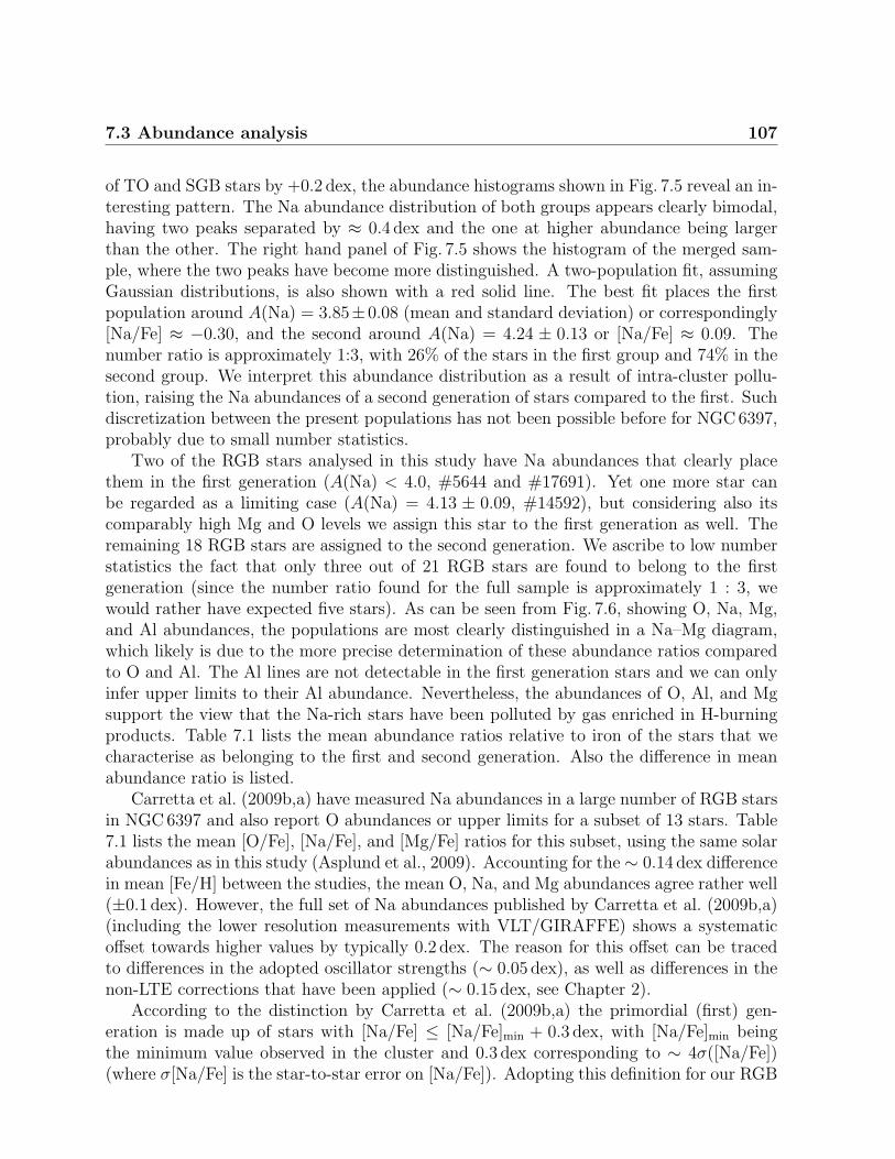
7.3 Abundance analysis 107
of TO and SGB stars by +0.2 dex, the abundance histograms shown in Fig. 7.5 reveal an in-teresting pattern. The Na abundance distribution of both groups appears clearly bimodal,having two peaks separated by ≈ 0.4 dex and the one at higher abundance being largerthan the other. The right hand panel of Fig. 7.5 shows the histogram of the merged sam-ple, where the two peaks have become more distinguished. A two-population fit, assumingGaussian distributions, is also shown with a red solid line. The best fit places the firstpopulation around A(Na) = 3.85±0.08 (mean and standard deviation) or correspondingly[Na/Fe] ≈ −0.30, and the second around A(Na) = 4.24 ± 0.13 or [Na/Fe] ≈ 0.09. Thenumber ratio is approximately 1:3, with 26% of the stars in the first group and 74% in thesecond group. We interpret this abundance distribution as a result of intra-cluster pollu-tion, raising the Na abundances of a second generation of stars compared to the first. Suchdiscretization between the present populations has not been possible before for NGC6397,probably due to small number statistics.
Two of the RGB stars analysed in this study have Na abundances that clearly placethem in the first generation (A(Na) < 4.0, #5644 and #17691). Yet one more star canbe regarded as a limiting case (A(Na) = 4.13 ± 0.09, #14592), but considering also itscomparably high Mg and O levels we assign this star to the first generation as well. Theremaining 18 RGB stars are assigned to the second generation. We ascribe to low numberstatistics the fact that only three out of 21 RGB stars are found to belong to the firstgeneration (since the number ratio found for the full sample is approximately 1 : 3, wewould rather have expected five stars). As can be seen from Fig. 7.6, showing O, Na, Mg,and Al abundances, the populations are most clearly distinguished in a Na–Mg diagram,which likely is due to the more precise determination of these abundance ratios comparedto O and Al. The Al lines are not detectable in the first generation stars and we can onlyinfer upper limits to their Al abundance. Nevertheless, the abundances of O, Al, and Mgsupport the view that the Na-rich stars have been polluted by gas enriched in H-burningproducts. Table 7.1 lists the mean abundance ratios relative to iron of the stars that wecharacterise as belonging to the first and second generation. Also the difference in meanabundance ratio is listed.
Carretta et al. (2009b,a) have measured Na abundances in a large number of RGB starsin NGC6397 and also report O abundances or upper limits for a subset of 13 stars. Table7.1 lists the mean [O/Fe], [Na/Fe], and [Mg/Fe] ratios for this subset, using the same solarabundances as in this study (Asplund et al., 2009). Accounting for the ∼ 0.14 dex differencein mean [Fe/H] between the studies, the mean O, Na, and Mg abundances agree rather well(±0.1 dex). However, the full set of Na abundances published by Carretta et al. (2009b,a)(including the lower resolution measurements with VLT/GIRAFFE) shows a systematicoffset towards higher values by typically 0.2 dex. The reason for this offset can be tracedto differences in the adopted oscillator strengths (∼ 0.05 dex), as well as differences in thenon-LTE corrections that have been applied (∼ 0.15 dex, see Chapter 2).
According to the distinction by Carretta et al. (2009b,a) the primordial (first) gen-eration is made up of stars with [Na/Fe] ≤ [Na/Fe]min + 0.3 dex, with [Na/Fe]min beingthe minimum value observed in the cluster and 0.3 dex corresponding to ∼ 4σ([Na/Fe])(where σ[Na/Fe] is the star-to-star error on [Na/Fe]). Adopting this definition for our RGB
1087. Tracing the evolution of NGC 6397 through the chemical composition of its
stellar populations
−0.4
−0.2
0.0
0.2
0.4
[Na/
Fe]
0.2 0.3 0.4 0.5 0.6[Mg/Fe]
0.2 0.4 0.6 0.8[O/Fe]
0.0
0.2
0.4
0.6
0.8
[Al/
Fe]
Figure 7.6: Na, Mg, and Al abundances for 21 stars and O abundances for 17 stars. Thethree Na-poor stars that we assign to the first generation are marked with blue squares.
sample, the first generation would consist of the same three stars, ([Na/Fe]min = −0.34).All the other sample stars are then considered as second-generation stars. Further, theauthors define an extreme component among second generation stars, if present, as starshaving [O/Na] < −0.9 (or [O/Na] < −1.03, adopting the solar abundances of Asplundet al. (2009). For NGC6397, none of the 13 targets analysed by Carretta et al. (2009a)fall in the extreme component according to this definition and the same is true for oursample. In numbers, Carretta et al. (2009a) find that 25±13% and 75±22% of their fullsample of stars in NGC6397 belong to the primordial and intermediate components, re-spectively, which agrees very well with our results (26% and 74%). Finally, we have alsoinspected the Na abundance histogram of the full Carretta et al. (2009b) sample, to seeif the same double-peaked distribution as in Fig. 7.5 can be distinguished. This is not thecase however, which we believe is likely due to the larger measurement errors (typically∼ 0.1 dex, according to their estimate, compared to ∼ 0.05 dex in our study), stemmingfrom their lower spectral quality. Obviously, the possibility that the bimodality seen inour abundance data is artificial and not representative of the true distribution cannot becompletely ruled out. This is unlikely though, especially considering that the two samples(TO+SGB and RGB) show a very similar pattern.
Fig. 7.7 compares the abundance ratios of our cluster targets to halo field data. Asexpected, we see that the [Na/Fe] ratio of the first generation is in good agreement with
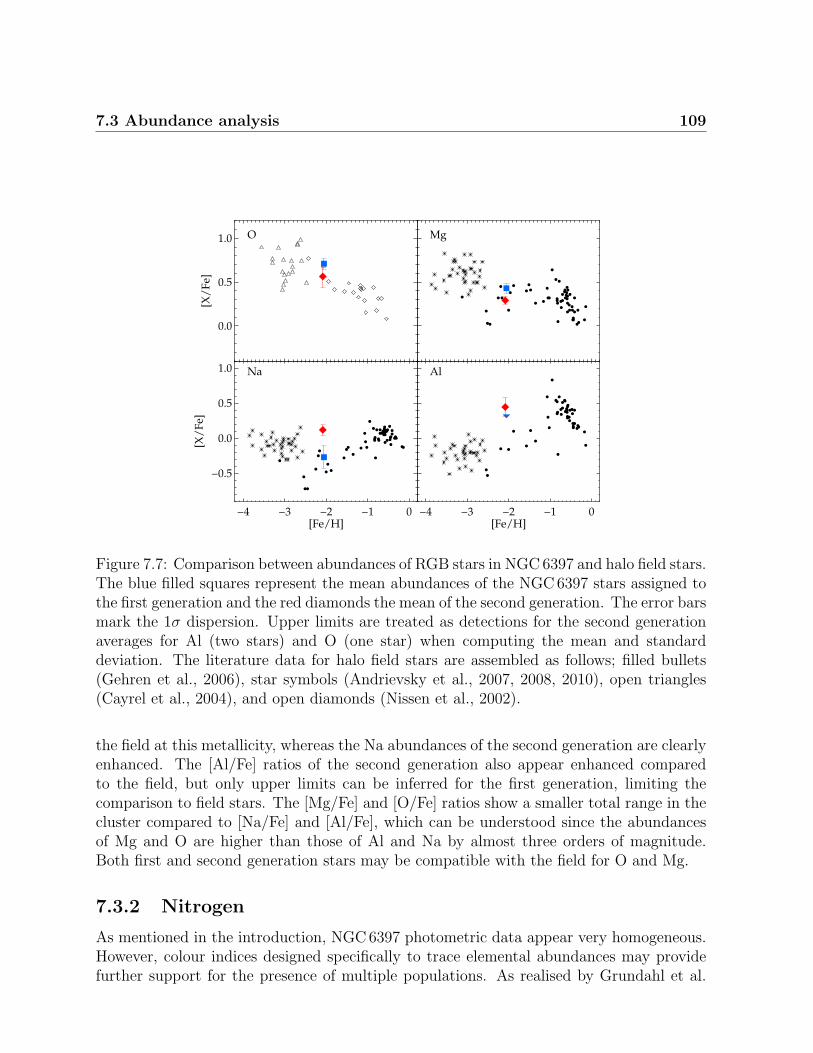
7.3 Abundance analysis 109
−4 −3 −2 −1 0[Fe/H]
−0.5
0.0
0.5
1.0
[X/
Fe]
Na
−4 −3 −2 −1 0[Fe/H]
Al
0.0
0.5
1.0
[X/
Fe]
O
Mg
Figure 7.7: Comparison between abundances of RGB stars in NGC 6397 and halo field stars.The blue filled squares represent the mean abundances of the NGC6397 stars assigned tothe first generation and the red diamonds the mean of the second generation. The error barsmark the 1σ dispersion. Upper limits are treated as detections for the second generationaverages for Al (two stars) and O (one star) when computing the mean and standarddeviation. The literature data for halo field stars are assembled as follows; filled bullets(Gehren et al., 2006), star symbols (Andrievsky et al., 2007, 2008, 2010), open triangles(Cayrel et al., 2004), and open diamonds (Nissen et al., 2002).
the field at this metallicity, whereas the Na abundances of the second generation are clearlyenhanced. The [Al/Fe] ratios of the second generation also appear enhanced comparedto the field, but only upper limits can be inferred for the first generation, limiting thecomparison to field stars. The [Mg/Fe] and [O/Fe] ratios show a smaller total range in thecluster compared to [Na/Fe] and [Al/Fe], which can be understood since the abundancesof Mg and O are higher than those of Al and Na by almost three orders of magnitude.Both first and second generation stars may be compatible with the field for O and Mg.
7.3.2 Nitrogen
As mentioned in the introduction, NGC 6397 photometric data appear very homogeneous.However, colour indices designed specifically to trace elemental abundances may providefurther support for the presence of multiple populations. As realised by Grundahl et al.

1107. Tracing the evolution of NGC 6397 through the chemical composition of its
stellar populations
(2002a), the strength of the Stromgren c1-index can be used as a tracer of the N abundance,since the u-filter involved in constructing this index covers the 336 nm NH features. Later,Yong et al. (2008a) empirically defined a more suitable index for the purpose, cy = c1 −(b− y), which removes much of the temperature sensitivity of c1. The top panel of Fig. 7.8shows a V − cy diagram, in which we have marked the first and second generation targetsin this study with different symbols. We also add the RGB targets analysed by Lind et al.(2009b), assigning stars with A(Na) < 4.0 to the first generation and A(Na) > 4.0 to thesecond. The clear separation between the generations visible in Fig. 7.8 indicates that alsotheir N abundances are affected. Such a correlation between cy-index and light elementabundances was recently illustrated also by Milone et al. (2010) for the more metal-richglobular cluster NGC 6752. In both clusters the first generation of stars seem to populate atight, blue RGB sequence in this colour index, and the second generation a more dispersed,red sequence.
In the bottom panel of Fig. 7.8 we have extracted a box centred on the middle RGB andproduced a histogram of the cy index. The magnitude cuts are applied to reduce remainingbias due to temperature effects. Again, we see a two-peaked histogram, very similar to theone obtained for Na abundance. The best fit returns the peak positions at cy = −0.341and cy = −0.306, with a size relationship of 25% and 75% for the left and right peak,in excellent agreement with previously inferred number fractions for the first and secondstellar generation (see Sect. 7.3.1).
We may estimate the corresponding difference in [N/Fe] abundance with the theoreti-cal calculations (using synthetic colours) by Onehag et al. (2009), giving an approximatesensitivity of δcy/δ[N/Fe] = 0.04 for stars in the same Teff and log g-ranges in NGC 6752.A somewhat stronger sensitivity, 0.06, was found by Yong et al. (2008a) who empiricallycorrelated spectroscopic N abundances with cy-colour for the same stars. This cluster hasslightly higher metallicity, but it still serves as an order of magnitude estimate. The typical∆[N/Fe] between stars of the first and second generation thus lies in the range 1–1.5 dex.This is consistent with spectroscopic N measurements by Carretta et al. (2005), who foundthat six out of nine SGB stars are strongly enhanced in [N/Fe] compared to the remainingsample, by as much as 1.5 dex. Pasquini et al. (2008) found all three stars in their sampleto be highly N-enriched compared to the field. Spectroscopic N measurements for a largesample of stars in NGC6397 is obviously desirable.
7.3.3 α and iron-peak elements
Globular clusters are generally very homogeneous in α and iron-peak elements, with theexceptions of peculiar clusters such as ω Cen. In NGC6397, the star-to-star scatter in[Fe/H] in our RGB sample is extremely small, only 0.03 dex, when basing the iron abun-dance on singly ionised lines. Fe I line abundances show a slight decreasing trend withdecreasing effective temperature, which is not seen in Fe II line abundances. The samepattern is seen for [Ti/Fe] and [Cr/Fe] ratios, and may indicate that the temperature scalecontains a small systematic bias (∼ 50K over a total range of 500K) or that non-LTEand/or 3D effects have minor differential effects. In Table 7.1, the reported Fe, Ti, and Cr
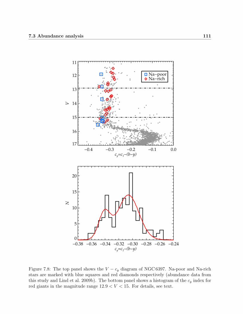
7.3 Abundance analysis 111
−0.4 −0.3 −0.2 −0.1 0.0cy=c1−(b−y)
17
16
15
14
13
12
11V
Na−poorNa−rich
−0.38 −0.36 −0.34 −0.32 −0.30 −0.28 −0.26 −0.24cy=c1−(b−y)
0
5
10
15
20
N
Figure 7.8: The top panel shows the V − cy diagram of NGC6397. Na-poor and Na-richstars are marked with blue squares and red diamonds respectively (abundance data fromthis study and Lind et al. 2009b). The bottom panel shows a histogram of the cy index forred giants in the magnitude range 12.9 < V < 15. For details, see text.
1127. Tracing the evolution of NGC 6397 through the chemical composition of its
stellar populations
abundances are all based only on singly ionised lines. The abundances of Mn, Co, Cu, andZn are based on one rather weak neutral line, which likely explains the larger star-to-starscatter in these abundances.
In general, the α and iron-peak elements show the expected pattern, in agreement withthe halo field at this metallicity. Ca, Si, Ti, and Sc are overabundant by 0.1 − 0.3 dex,whereas the iron-peak elements Cr, Co, Ni, and Zn are approximately solar. The odd-zelements Mn and Cu are strongly under-abundant compared to the Sun, and the low valuewe have inferred for Cu (< [Cu/Fe] >= −0.89) is slightly below the values recently inferredfor field dwarfs at this metallicity by Primas & Sobeck (2008). The mean Mn abundance(< [Mn/Fe] >= −0.54) is very similar to the LTE abundances inferred by Bergemann &Gehren (2008), but as shown in that study, non-LTE corrections for Mn are positive andrather substantial.
As can also be seen in Table 7.1, there is no significant difference (i.e. > 2σ) between themean abundances of intermediate mass (heavier than Al) and iron-peak elements betweenthe stars that we characterise as belonging to the first and second generation.
7.3.4 Neutron capture elements
Metal-poor halo field stars are known to display a large scatter in some of the neutron cap-ture elements, which cannot be explained by observational uncertainties (see e.g. Barklemet al. 2005; Burris et al. 2000). Stars within a globular cluster are generally much morehomogeneous in their heavy element abundances, as shown by for example (James et al.,2004) for NGC6397, NGC6752, and 47Tuc and by Yong et al. (2008b) for M4 and M5.This is confirmed by our study, with low abundance dispersions found for Y, Zr, Ba, Ce, Nd,and Eu. The mean abundance ratios we derive for [Y/Fe] = −0.26 and [Ba/Fe] = −0.08are in reasonable agreement with previous estimates for the cluster (in addition to the val-ues listed in Table 7.1, James et al. 2004 determined [Y/Fe] = −0.2 and [Ba/Fe] = −0.17for stars at the base of the RGB). The other elements have not been previously anal-ysed in NGC 6397. Comparing to the values determined for the higher metallicity clusterNGC 6752 by Yong et al. (2005), we see good agreement between Zr, Ba, Ce, Nd, and Euabundances. However, for Zr this is partly coincidental; accounting for differences in theadopted oscillator strength for the Zr II line at 511.2 nm, our abundance ratio would be0.3 dex lower. A similar difference is seen when comparing the estimates for [Y/Fe]. Itthus seems that the two clusters are very similar in heavy neutron capture elements havingZ > 56, whereas the lighter Z = 39− 40 elements are 0.3 dex less abundant in NGC 6397.
According to Burris et al. (2000), Y, Zr, Ba, and Ce are all mainly s-process elements(72-85% s-process contribution), whereas Nd is approximately half r-process, half s-process.Eu is a almost a pure (97%) r-process element. For the first time we determine the [Ba/Eu]ratio in this cluster, and the value we infer (−0.49), fall rather close to the scaled solarr-process of −0.81 (the scaled s-process value is 1.45). The same is true for the [Zr/Eu],[Ce/Eu], and [Nd/Eu] ratios, whereas [Y/Fe] even is slightly below the expectation frompure r-process contribution. It thus seems that chemical enrichment by core-collapse su-pernovae may be sufficient to explain the observed heavy element abundances, and that
7.3 Abundance analysis 113
contribution from AGB stars has been limited.
The two stellar generations are very similar in the measured neutron-capture elements(see Table 7.1). Only the [Y/Fe] ratio is higher by ∼ 3σ in the second generation. Thedifference (0.04 dex) is, however, too small to be convincing. A comparison to halo fieldstars does not provide much information, since the stars in the field are highly scattered.The abundances we find for NGC 6397 are well within the ranges found e.g. by Francoiset al. (2007) for a sample of metal-poor field giants.
7.3.5 Helium
If the second generation stars in globular clusters indeed have been enriched in nucleosyn-thesis products connected to hydrogen-burning, they should also have a higher He contentthan their first generation counterparts, although we may only speculate on the exactamount.
Recently, di Criscienzo et al. (2010) used the accurate, proper-motion cleaned HSTphotometry of Richer et al. (2008) to measure the width of the MS in NGC6397 andconstrain the possible helium spread in the cluster. Under the assumption that 70% of thestars belong to the second generation and have a C+N+O enhancement as suggested byspectroscopic observations (∆[(C + N + O)/Fe] ∼ 0.25 according to Carretta et al. 2005),they conclude that the cluster must be very uniform in He abundance, implying only∆Y = 0.02 between first and second generation. When allowing for higher [(C+N+O)/Fe]over-abundances, a broader spread in helium (∆Y up to 0.04) is compatible with thetightness of the MS. Here we will attempt to constrain this difference by spectroscopicarguments instead.
The He abundance cannot be measured directly in late-type stars, but it neverthelessinfluences the emerging stellar spectrum. The effects of helium-enrichment in a cool stellaratmosphere have been investigated by Stromgren et al. (1982), who found that changes inthe helium-to-hydrogen ratio in F type dwarfs affect the mean molecular weight of the gasand have impact on the gas pressure. However, helium contributes only negligible to lineand continuous opacity in a cool atmosphere and does not provide free electrons. Therefore,Stromgren et al. (1982) concluded and demonstrated that a helium-enrichment can bemapped merely as a shift in surface gravity, i.e. a helium-enriched atmosphere is similarto a helium-normal atmosphere with a higher surface gravity, in terms of temperaturestructure and electron pressure structure. Stars with identical T and Pe structures andthe same ratio of metals-to-hydrogen also have identical spectra. The calculation of thenecessary shift in surface gravity is given by the relation (see equivalent Eq. 12 in Stromgrenet al. 1982).
log g′′ = log g′ + log
((1 + 4× y′)(1 + y′′)
(1 + 4× y′′)(1 + y′)
)(7.1)
Here log g′ is the surface gravity of the model with helium-to-hydrogen ratio y′ =NHe/NH and analogously for the double-primed variables. We have tested whether the
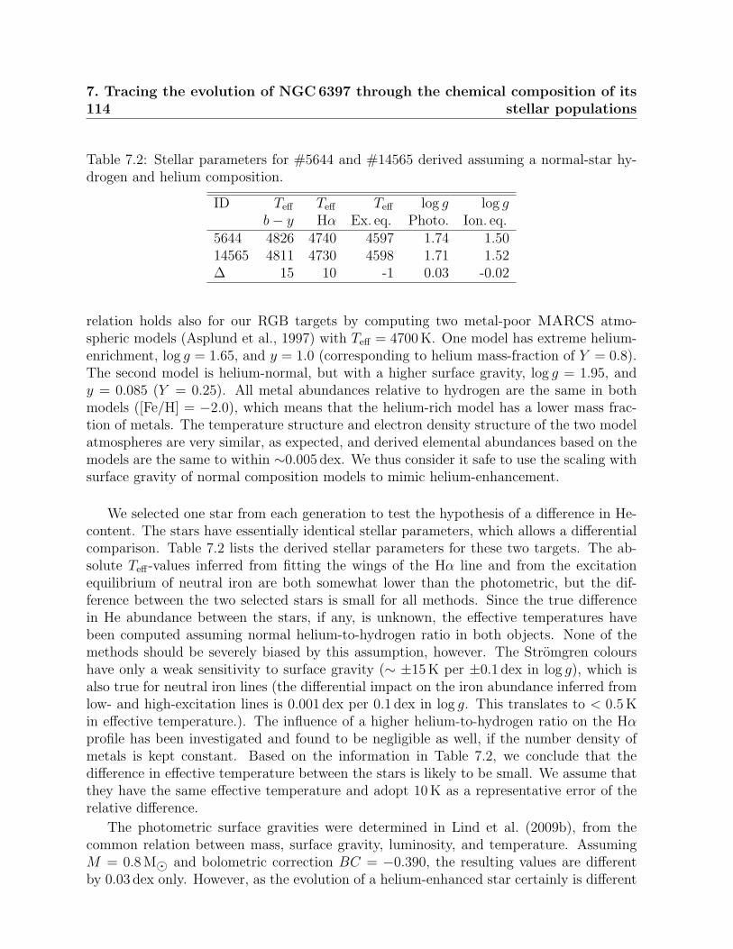
1147. Tracing the evolution of NGC 6397 through the chemical composition of its
stellar populations
Table 7.2: Stellar parameters for #5644 and #14565 derived assuming a normal-star hy-drogen and helium composition.
ID Teff Teff Teff log g log gb− y Hα Ex. eq. Photo. Ion. eq.
5644 4826 4740 4597 1.74 1.5014565 4811 4730 4598 1.71 1.52∆ 15 10 -1 0.03 -0.02
relation holds also for our RGB targets by computing two metal-poor MARCS atmo-spheric models (Asplund et al., 1997) with Teff = 4700 K. One model has extreme helium-enrichment, log g = 1.65, and y = 1.0 (corresponding to helium mass-fraction of Y = 0.8).The second model is helium-normal, but with a higher surface gravity, log g = 1.95, andy = 0.085 (Y = 0.25). All metal abundances relative to hydrogen are the same in bothmodels ([Fe/H] = −2.0), which means that the helium-rich model has a lower mass frac-tion of metals. The temperature structure and electron density structure of the two modelatmospheres are very similar, as expected, and derived elemental abundances based on themodels are the same to within ∼0.005 dex. We thus consider it safe to use the scaling withsurface gravity of normal composition models to mimic helium-enhancement.
We selected one star from each generation to test the hypothesis of a difference in He-content. The stars have essentially identical stellar parameters, which allows a differentialcomparison. Table 7.2 lists the derived stellar parameters for these two targets. The ab-solute Teff-values inferred from fitting the wings of the Hα line and from the excitationequilibrium of neutral iron are both somewhat lower than the photometric, but the dif-ference between the two selected stars is small for all methods. Since the true differencein He abundance between the stars, if any, is unknown, the effective temperatures havebeen computed assuming normal helium-to-hydrogen ratio in both objects. None of themethods should be severely biased by this assumption, however. The Stromgren colourshave only a weak sensitivity to surface gravity (∼ ±15K per ±0.1 dex in log g), which isalso true for neutral iron lines (the differential impact on the iron abundance inferred fromlow- and high-excitation lines is 0.001 dex per 0.1 dex in log g. This translates to < 0.5Kin effective temperature.). The influence of a higher helium-to-hydrogen ratio on the Hαprofile has been investigated and found to be negligible as well, if the number density ofmetals is kept constant. Based on the information in Table 7.2, we conclude that thedifference in effective temperature between the stars is likely to be small. We assume thatthey have the same effective temperature and adopt 10K as a representative error of therelative difference.
The photometric surface gravities were determined in Lind et al. (2009b), from thecommon relation between mass, surface gravity, luminosity, and temperature. AssumingM = 0.8 M and bolometric correction BC = −0.390, the resulting values are differentby 0.03 dex only. However, as the evolution of a helium-enhanced star certainly is different
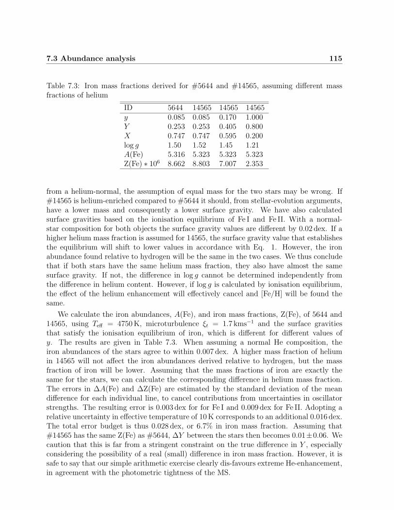
7.3 Abundance analysis 115
Table 7.3: Iron mass fractions derived for #5644 and #14565, assuming different massfractions of helium
ID 5644 14565 14565 14565y 0.085 0.085 0.170 1.000Y 0.253 0.253 0.405 0.800X 0.747 0.747 0.595 0.200log g 1.50 1.52 1.45 1.21A(Fe) 5.316 5.323 5.323 5.323Z(Fe) ∗ 106 8.662 8.803 7.007 2.353
from a helium-normal, the assumption of equal mass for the two stars may be wrong. If#14565 is helium-enriched compared to #5644 it should, from stellar-evolution arguments,have a lower mass and consequently a lower surface gravity. We have also calculatedsurface gravities based on the ionisation equilibrium of Fe I and Fe II. With a normal-star composition for both objects the surface gravity values are different by 0.02 dex. If ahigher helium mass fraction is assumed for 14565, the surface gravity value that establishesthe equilibrium will shift to lower values in accordance with Eq. 1. However, the ironabundance found relative to hydrogen will be the same in the two cases. We thus concludethat if both stars have the same helium mass fraction, they also have almost the samesurface gravity. If not, the difference in log g cannot be determined independently fromthe difference in helium content. However, if log g is calculated by ionisation equilibrium,the effect of the helium enhancement will effectively cancel and [Fe/H] will be found thesame.
We calculate the iron abundances, A(Fe), and iron mass fractions, Z(Fe), of 5644 and14565, using Teff = 4750 K, microturbulence ξt = 1.7 kms−1 and the surface gravitiesthat satisfy the ionisation equilibrium of iron, which is different for different values ofy. The results are given in Table 7.3. When assuming a normal He composition, theiron abundances of the stars agree to within 0.007 dex. A higher mass fraction of heliumin 14565 will not affect the iron abundances derived relative to hydrogen, but the massfraction of iron will be lower. Assuming that the mass fractions of iron are exactly thesame for the stars, we can calculate the corresponding difference in helium mass fraction.The errors in ∆A(Fe) and ∆Z(Fe) are estimated by the standard deviation of the meandifference for each individual line, to cancel contributions from uncertainties in oscillatorstrengths. The resulting error is 0.003 dex for for Fe I and 0.009 dex for Fe II. Adopting arelative uncertainty in effective temperature of 10K corresponds to an additional 0.016 dex.The total error budget is thus 0.028 dex, or 6.7% in iron mass fraction. Assuming that#14565 has the same Z(Fe) as #5644, ∆Y between the stars then becomes 0.01±0.06. Wecaution that this is far from a stringent constraint on the true difference in Y , especiallyconsidering the possibility of a real (small) difference in iron mass fraction. However, it issafe to say that our simple arithmetic exercise clearly dis-favours extreme He-enhancement,in agreement with the photometric tightness of the MS.
1167. Tracing the evolution of NGC 6397 through the chemical composition of its
stellar populations
In the cluster formation scenario described by Decressin et al. (2007a), with slow windsfrom rotating massive stars pollute the star forming gas, one expects an anti-correlationbetween helium and [O/Na] for second generation stars born out of a mixture of stellarejecta and pristine material. As can be seen in Fig. 13 of Decressin et al. (2007a), the smallvalue implied for ∆Y is fully compatible with the corresponding ∆ [O/Na] of 0.75 dexbetween #5644 and #14565. This good agreement persists over the whole mass rangeconsidered by Decressin et al. (2007a), i.e., for polluter stars with masses between 20 and120 M.
7.4 Consequences for the evolutionary scenario
We will now investigate if the abundance patterns we derived for NGC6397 can be ac-counted for in the framework of the so-called “wind of fast rotating massive stars” (WFRMS)scenario (e.g. Prantzos & Charbonnel 2006; Decressin et al. 2007a,b). In this scenario,second generation stars are formed from matter ejected through slow winds of individualmassive stars (M≥20 M), mixed locally with pristine interstellar gas. These massive starssupposedly reach the critical rotational velocity early on the MS phase, and loose signifi-cant mass and angular momentum by ejecting material in an equatorial disk. Due to deeprotational mixing, this material is enhanced in H-burning products produced in the stellarcore. When the stars explode as supernovae the previously ejected slow material can stillbe retained in the cluster and united with the inter-stellar medium that form the secondgeneration stars.
7.4.1 Method
We follow the same procedure as described in Decressin et al. (2007a), using the stellarmodels by Decressin et al. (2007b) that were computed for the metallicity of NGC6752([Fe/H]∼ −1.56), i.e. slightly higher than that of NGC6397 ([Fe/H]∼ −2.08). A differenceof this size should have no impact on our conclusions (Ekstrom et al., 2008). However,the enrichment history of the two clusters certainly differ to some extent, which must beconsidered in the analysis. Especially, the full range in O abundance is twice as large inNGC 6752 (0.8 dex, Yong et al. 2003) compared to NGC6397 (0.4 dex, see Fig. 7.6). Also,NGC 6752 has a broadened main sequence (Milone et al., 2010) and an extended horizontalbranch, indicating a larger variation in the He content.
When establishing the recycling process of NGC 6752, Decressin et al. (2007a) took intoaccount all the material ejected by massive stars rotating at critical velocity, both on themain sequence and during the first part of the central He-burning phase2. This allowedthe build up of extreme abundance anomalies in both O and Na, and also lead to highHe-enrichment for the “extreme component” of second generation stars. As discussed in
2Due to strong mechanical mass loss fast rotating stars actually evolve away from the critical limitduring the central He-burning phase, before the He-burning products contaminate the slow wind component(Decressin et al., 2007b; Ekstrom et al., 2008).
7.4 Consequences for the evolutionary scenario 117
Sect. 7.3.1 and 7.3.5, such extreme anomalies appear to be lacking in NGC 6397, and thesecond generation stars are probably only mildly overabundant in He. Consequently, weassume that only the slow winds ejected on the main sequence by fast rotating massivestars are recycled into the second generation and we neglect the material that is lost duringthe luminous blue variable phase. As discussed in Sect. 7.4.5 this may have some impacton the total mass budget, although most of the mass loss through the slow mechanicalwinds occurs while the fast rotating stars are on the main sequence (in the case of a60 M rotating at critical velocity, 20 and 7 M are lost through the mechanical windon and slightly after the main sequence, respectively). We will not venture to discuss indetail the underlying reason for the different observed abundance patterns in NGC6752and NGC6397, but one may speculate that different initial masses of these clusters haveplayed a role.
7.4.2 Amount of dilution between massive star ejecta and pris-tine gas
The star-to-star spread in light element abundances observed in globular clusters todayimplies that all the material ejected by the first generation massive stars was not fullymixed before being recycled into the second stellar generation. Additionally the observedbehaviours of both O and Li pinpoints the formation of second generation stars in thevicinity of individual massive stars from their slow winds mixed with pristine interstellarmatter.
As explained in Decressin et al. (2007a) we may use the observed Li-Na anti-correlationto estimate the amount of dilution between the massive star ejecta that are totally void ofLi and the pristine intra-cluster gas left after the formation of first generation stars, whoseLi abundance is assumed to be equal to the primordial (Big Bang) value. We furtherassume that the slow wind of each individual massive star undergoes locally a variabledilution with time. In the early main sequence phase, the stellar ejecta encounter morepristine gas and are hence more diluted than the matter ejected later. As the stellar windsbecome more Na-rich later in the course of the evolution of a massive polluter, the Li-Naanti-correlation builds up naturally: second generation low-mass stars with a relativelyhigh Li content and a relatively low Na abundance are created first, while stars formedfrom matter ejected later have less Li and more Na.
In Fig. 7.9 we present theoretical predictions for the Li and Na abundance variationsin the resulting material out of which second generation low-mass stars are assumed toform. The tracks shown correspond to the cases of the ejecta of the 20 and 120 M modelsby Decressin et al. (2007b) for different values (0.2, 0.4, 0.6, and 0.8) of the minimumdilution (along individual tracks dilution decreases from 1 down to this minimum valueas the polluter star evolves). Predictions for polluters with different initial masses wouldfill the whole space between 20 and 120 M tracks. The initial (pristine) [Na/Fe] value isassumed to be the average that we find for first generation stars (i.e., −0.3; see Sect. 7.3.1).For Li we consider the value from WMAP and Big Bang nucleosynthesis (A(Li) = 2.72
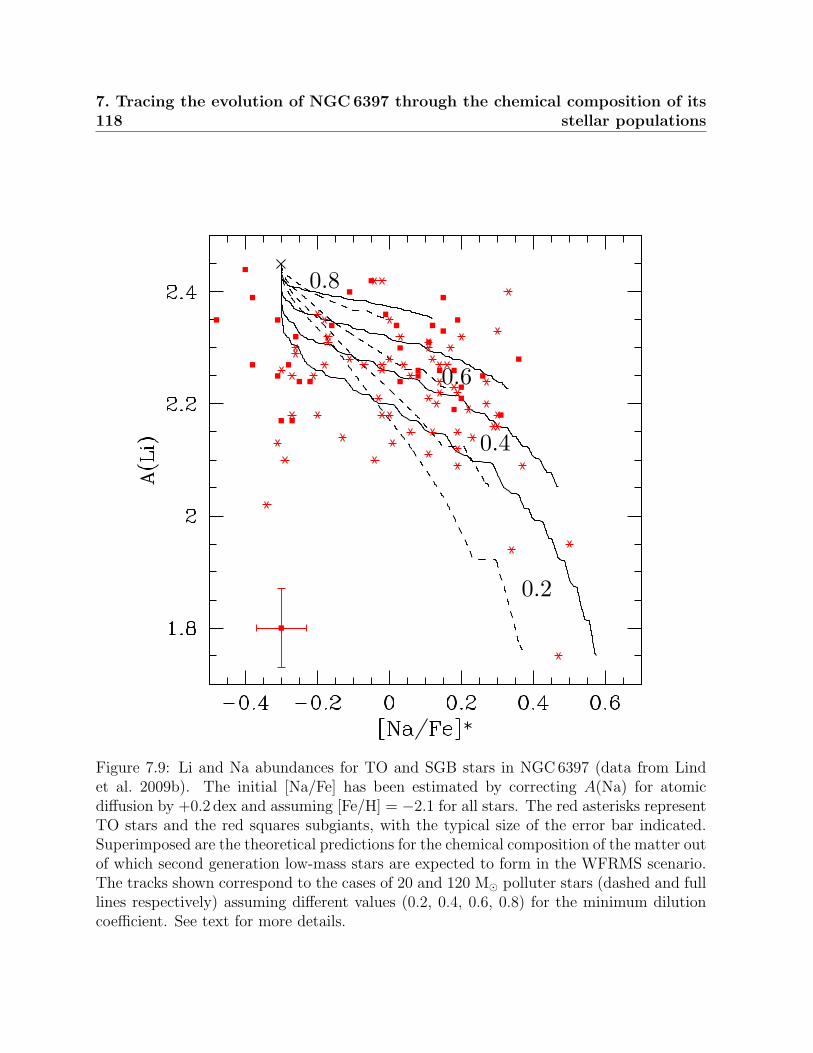
1187. Tracing the evolution of NGC 6397 through the chemical composition of its
stellar populations
0.8
0.6
0.4
0.2
Figure 7.9: Li and Na abundances for TO and SGB stars in NGC6397 (data from Lindet al. 2009b). The initial [Na/Fe] has been estimated by correcting A(Na) for atomicdiffusion by +0.2 dex and assuming [Fe/H] = −2.1 for all stars. The red asterisks representTO stars and the red squares subgiants, with the typical size of the error bar indicated.Superimposed are the theoretical predictions for the chemical composition of the matter outof which second generation low-mass stars are expected to form in the WFRMS scenario.The tracks shown correspond to the cases of 20 and 120 M polluter stars (dashed and fulllines respectively) assuming different values (0.2, 0.4, 0.6, 0.8) for the minimum dilutioncoefficient. See text for more details.
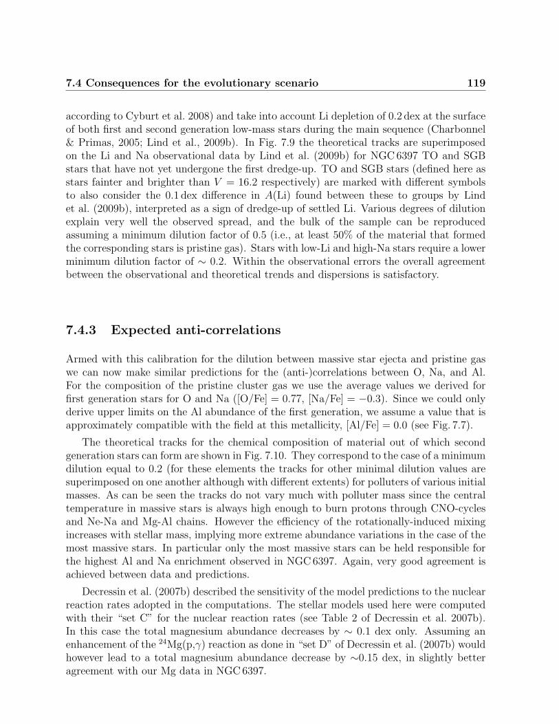
7.4 Consequences for the evolutionary scenario 119
according to Cyburt et al. 2008) and take into account Li depletion of 0.2 dex at the surfaceof both first and second generation low-mass stars during the main sequence (Charbonnel& Primas, 2005; Lind et al., 2009b). In Fig. 7.9 the theoretical tracks are superimposedon the Li and Na observational data by Lind et al. (2009b) for NGC 6397 TO and SGBstars that have not yet undergone the first dredge-up. TO and SGB stars (defined here asstars fainter and brighter than V = 16.2 respectively) are marked with different symbolsto also consider the 0.1 dex difference in A(Li) found between these to groups by Lindet al. (2009b), interpreted as a sign of dredge-up of settled Li. Various degrees of dilutionexplain very well the observed spread, and the bulk of the sample can be reproducedassuming a minimum dilution factor of 0.5 (i.e., at least 50% of the material that formedthe corresponding stars is pristine gas). Stars with low-Li and high-Na stars require a lowerminimum dilution factor of ∼ 0.2. Within the observational errors the overall agreementbetween the observational and theoretical trends and dispersions is satisfactory.
7.4.3 Expected anti-correlations
Armed with this calibration for the dilution between massive star ejecta and pristine gaswe can now make similar predictions for the (anti-)correlations between O, Na, and Al.For the composition of the pristine cluster gas we use the average values we derived forfirst generation stars for O and Na ([O/Fe] = 0.77, [Na/Fe] = −0.3). Since we could onlyderive upper limits on the Al abundance of the first generation, we assume a value that isapproximately compatible with the field at this metallicity, [Al/Fe] = 0.0 (see Fig. 7.7).
The theoretical tracks for the chemical composition of material out of which secondgeneration stars can form are shown in Fig. 7.10. They correspond to the case of a minimumdilution equal to 0.2 (for these elements the tracks for other minimal dilution values aresuperimposed on one another although with different extents) for polluters of various initialmasses. As can be seen the tracks do not vary much with polluter mass since the centraltemperature in massive stars is always high enough to burn protons through CNO-cyclesand Ne-Na and Mg-Al chains. However the efficiency of the rotationally-induced mixingincreases with stellar mass, implying more extreme abundance variations in the case of themost massive stars. In particular only the most massive stars can be held responsible forthe highest Al and Na enrichment observed in NGC6397. Again, very good agreement isachieved between data and predictions.
Decressin et al. (2007b) described the sensitivity of the model predictions to the nuclearreaction rates adopted in the computations. The stellar models used here were computedwith their “set C” for the nuclear reaction rates (see Table 2 of Decressin et al. 2007b).In this case the total magnesium abundance decreases by ∼ 0.1 dex only. Assuming anenhancement of the 24Mg(p,γ) reaction as done in “set D” of Decressin et al. (2007b) wouldhowever lead to a total magnesium abundance decrease by ∼0.15 dex, in slightly betteragreement with our Mg data in NGC6397.
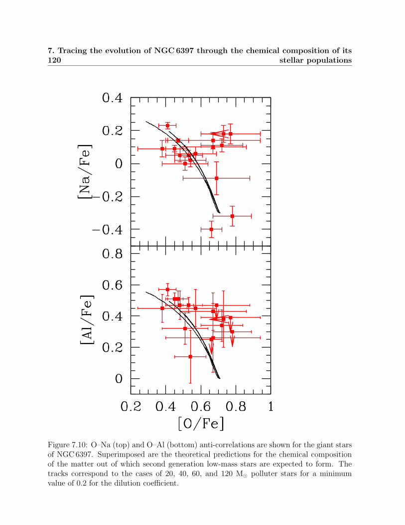
1207. Tracing the evolution of NGC 6397 through the chemical composition of its
stellar populations
Figure 7.10: O–Na (top) and O–Al (bottom) anti-correlations are shown for the giant starsof NGC 6397. Superimposed are the theoretical predictions for the chemical compositionof the matter out of which second generation low-mass stars are expected to form. Thetracks correspond to the cases of 20, 40, 60, and 120 M polluter stars for a minimumvalue of 0.2 for the dilution coefficient.
7.4 Consequences for the evolutionary scenario 121
0.8
0.2
Figure 7.11: ratio for second generation stars.] Expected anti-correlation between helium (in mass
fraction) and [O/Na] for second generation stars (at birth) born out of material ejectedthrough slow winds of massive stars and diluted with gas of pristine composition. Thetracks correspond to the cases of 20 and 120 M polluter stars (dashed and full lines
respectively) assuming different values (0.2 and 0.8) for the minimum dilution coefficient.See text for more details. The shaded regions indicate the star-to-star abundancedifferences derived in Sect. 7.3 for #5644 and #14565 and related uncertainties
(∆[O/Na] = 0.75 and ∆Y < 0.07).

1227. Tracing the evolution of NGC 6397 through the chemical composition of its
stellar populations
7.4.4 He content
We can now make predictions for the helium spread expected within the WFRMS scenariowith the assumptions described above for the specific case of NGC6397. Fig. 7.11 showspredicted variation in He mass fraction as a function of the [O/Na] ratio. Also shown arethe values estimated in Sect. 7.3 for #5644 and #14565. We see that the theoretical heliumvariation corresponding to a ∆[O/Na] of 0.75 is less than 0.04, fully compatible with thespectroscopic estimate.
When assuming a “standard” IMF (slope of 2.35) for the massive polluter stars andtaking into account the variable dilution process described in Sect. 7.4.2, we obtain that∼ 70% of second generation stars should be born with an helium mass fraction that is0.02 higher than first generation stars. In addition, about 5-10% of second generationstars are expected to be born within the range Y = 0.35− 0.39. The resulting dispersionin Y is compatible with the constraints obtained from the width of the main sequence(∆Y < 0.04).
7.4.5 Initial cluster mass
As discussed in Sect. 7.3.1, about 74% of the long-lived low-mass stars still present today inNGC 6397 belong to the so-called second generation, while about 26% were born with thesame chemical composition as the massive polluters. Prantzos & Charbonnel (2006) andDecressin et al. (2007a,b) have shown that such high number ratio of second generationstars requires either a very flat IMF for the first generation massive stars, or that a verylarge number of first generation low-mass stars have escaped the cluster. This secondoption is favoured by recent finding that the fraction of halo field stars initially formedwithin globular clusters could be as large as 50% (Martell & Grebel, 2010).
We thus follow here the second scenario, assuming in addition that the first stellargeneration consists of stars with initial masses between 0.1 and 120 M, while the secondgeneration consists only of long-lived low-mass stars (0.1 – 0.8 M). The latter assumptionobviously minimises the constraints on the mass budget. We use a Salpeter IMF for themassive stars of the first generation, but assume that the present-day log-normal distribu-tion derived by Paresce & De Marchi (2000) reflects the IMF of the long lived low-massstars of both first and second generation.
We can then derive the amount of first generation long-lived stars that must have beenlost in order to fit the high ratio of second to first generation stars (3:1) found in NGC6397.As we consider pollution by massive star ejecta released on the main sequence only, wehave less polluter material to form new stars than in the case of NGC6752 studied inDecressin et al. (2007a). This effect is partially compensated by the higher dilution neededto reproduce the Li-Na anti-correlation as we form more second generation stars per unitmass released into slow winds. Finally, we find that about 90% of first generation low-massstars must have been lost by NGC6397, probably during the early event of gas expulsionby supernovae (see Decressin et al. 2010). The initial mass of NGC 6397 must thus havebeen ∼ 10 times higher than its present day mass.
7.5 Conclusions 123
7.5 Conclusions
In this study of RGB stars in the globular cluster NGC6397, we have demonstrated thepossibility to distinguish between the present stellar generations spectroscopically, by mak-ing use of a double-peaked histogram of Na abundances. A two-population fit returns aNa abundance similar to the halo field for 26% of the stars, which we characterise as be-longing to a first generation, whereas the remaining 74% (i.e. second generation) showhighly elevated Na abundances. This bimodal abundance signature should be verified foran extended sample, and similar histograms may be possible to produce also for N and Alabundance, for which large spreads are present in globular clusters. The abundance spreadsare smaller for O and Mg, making the task more challenging. Highly precise abundanceanalysis, with small statistical error bars will be necessary to distinguish such patterns, ifpresent.
Based on 17 different elements heavier than Al, we conclude that there is no supportfor α, iron-peak or neutron-capture abundances to be significantly different between thestellar generations. We have also estimated the difference in He abundance between twostars of each generation by enforcing the mass fraction of iron to be same within the errorbars of the analysis. Such small (if any) difference in He is expected from models of clusterself-enrichment and also supported by the tightness of the main sequence of NGC6397.The same exercise should be performed for other globular clusters, especially those showingmultiple main sequences, hopefully bringing us closer to identifying the process responsiblefor early cluster pollution.
Finally we have shown that the abundance patterns observed in NGC6397 can be wellreproduced within the “wind of fast rotating massive stars” scenario. Based on the Li-Narelation we could deduce the dilution factors between the ejecta of massive polluters andinterstellar gas of pristine composition. The observed ratio of second to first generationstars was used to estimate the number fraction of first generation long-lived low-mass starsthat must have been lost by NGC 6397, and thus the initial mass of this globular cluster.Although we did not make explicit comparisons with the yields of AGB stars, we expectthis scenario to be able to account equally well for the observed abundance patterns of thisglobular cluster.
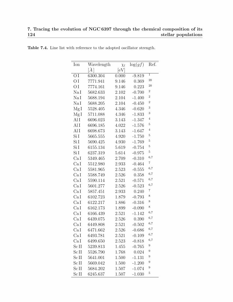
1247. Tracing the evolution of NGC 6397 through the chemical composition of its
stellar populations
Table 7.4. Line list with reference to the adopted oscillator strength.
Ion Wavelength χl log(gf) Ref.[A ] [eV]
O I 6300.304 0.000 -9.819 1
OI 7771.941 9.146 0.369 20
OI 7774.161 9.146 0.223 20
Na I 5682.633 2.102 -0.700 2
Na I 5688.194 2.104 -1.400 2
Na I 5688.205 2.104 -0.450 2
Mg I 5528.405 4.346 -0.620 3
Mg I 5711.088 4.346 -1.833 3
Al I 6696.023 3.143 -1.347 4
Al I 6696.185 4.022 -1.576 5
Al I 6698.673 3.143 -1.647 4
Si I 5665.555 4.920 -1.750 5
Si I 5690.425 4.930 -1.769 5
Si I 6155.134 5.619 -0.754 5
Si I 6237.319 5.614 -0.975 5
Ca I 5349.465 2.709 -0.310 6,7
Ca I 5512.980 2.933 -0.464 7
Ca I 5581.965 2.523 -0.555 6,7
Ca I 5588.749 2.526 0.358 6,7
Ca I 5590.114 2.521 -0.571 6,7
Ca I 5601.277 2.526 -0.523 6,7
Ca I 5857.451 2.933 0.240 7
Ca I 6102.723 1.879 -0.793 8
Ca I 6122.217 1.886 -0.316 8
Ca I 6162.173 1.899 -0.090 8
Ca I 6166.439 2.521 -1.142 6,7
Ca I 6439.075 2.526 0.390 6,7
Ca I 6449.808 2.521 -0.502 6,7
Ca I 6471.662 2.526 -0.686 6,7
Ca I 6493.781 2.521 -0.109 6,7
Ca I 6499.650 2.523 -0.818 6,7
Sc II 5239.813 1.455 -0.765 9
Sc II 5526.790 1.768 0.024 9
Sc II 5641.001 1.500 -1.131 9
Sc II 5669.042 1.500 -1.200 9
Sc II 5684.202 1.507 -1.074 9
Sc II 6245.637 1.507 -1.030 5
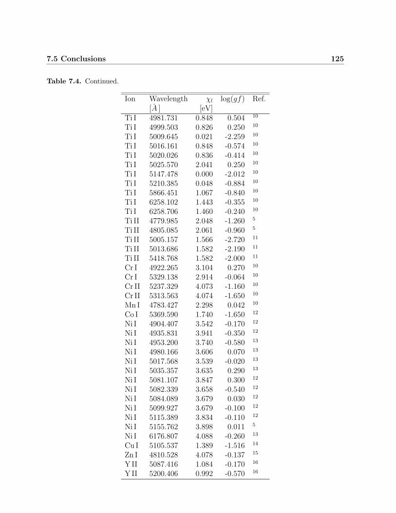
7.5 Conclusions 125
Table 7.4. Continued.
Ion Wavelength χl log(gf) Ref.[A ] [eV]
Ti I 4981.731 0.848 0.504 10
Ti I 4999.503 0.826 0.250 10
Ti I 5009.645 0.021 -2.259 10
Ti I 5016.161 0.848 -0.574 10
Ti I 5020.026 0.836 -0.414 10
Ti I 5025.570 2.041 0.250 10
Ti I 5147.478 0.000 -2.012 10
Ti I 5210.385 0.048 -0.884 10
Ti I 5866.451 1.067 -0.840 10
Ti I 6258.102 1.443 -0.355 10
Ti I 6258.706 1.460 -0.240 10
Ti II 4779.985 2.048 -1.260 5
Ti II 4805.085 2.061 -0.960 5
Ti II 5005.157 1.566 -2.720 11
Ti II 5013.686 1.582 -2.190 11
Ti II 5418.768 1.582 -2.000 11
Cr I 4922.265 3.104 0.270 10
Cr I 5329.138 2.914 -0.064 10
Cr II 5237.329 4.073 -1.160 10
Cr II 5313.563 4.074 -1.650 10
Mn I 4783.427 2.298 0.042 10
Co I 5369.590 1.740 -1.650 12
Ni I 4904.407 3.542 -0.170 12
Ni I 4935.831 3.941 -0.350 12
Ni I 4953.200 3.740 -0.580 13
Ni I 4980.166 3.606 0.070 13
Ni I 5017.568 3.539 -0.020 13
Ni I 5035.357 3.635 0.290 13
Ni I 5081.107 3.847 0.300 12
Ni I 5082.339 3.658 -0.540 12
Ni I 5084.089 3.679 0.030 12
Ni I 5099.927 3.679 -0.100 12
Ni I 5115.389 3.834 -0.110 12
Ni I 5155.762 3.898 0.011 5
Ni I 6176.807 4.088 -0.260 13
Cu I 5105.537 1.389 -1.516 14
Zn I 4810.528 4.078 -0.137 15
YII 5087.416 1.084 -0.170 16
YII 5200.406 0.992 -0.570 16
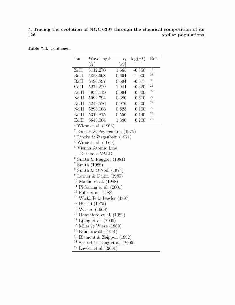
1267. Tracing the evolution of NGC 6397 through the chemical composition of its
stellar populations
Table 7.4. Continued.
Ion Wavelength χl log(gf) Ref.[A ] [eV]
Zr II 5112.270 1.665 -0.850 17
Ba II 5853.668 0.604 -1.000 18
Ba II 6496.897 0.604 -0.377 18
Ce II 5274.229 1.044 -0.320 21
Nd II 4959.119 0.064 -0.800 19
Nd II 5092.794 0.380 -0.610 19
Nd II 5249.576 0.976 0.200 19
Nd II 5293.163 0.823 0.100 19
Nd II 5319.815 0.550 -0.140 19
Eu II 6645.064 1.380 0.200 22
1 Wiese et al. (1966)2 Kurucz & Peytremann (1975)3 Lincke & Ziegenbein (1971)4 Wiese et al. (1969)5 Vienna Atomic Line
Database VALD6 Smith & Raggett (1981)7 Smith (1988)8 Smith & O’Neill (1975)9 Lawler & Dakin (1989)10 Martin et al. (1988)11 Pickering et al. (2001)12 Fuhr et al. (1988)13 Wickliffe & Lawler (1997)14 Bielski (1975)15 Warner (1968)16 Hannaford et al. (1982)17 Ljung et al. (2006)18 Miles & Wiese (1969)19 Komarovskii (1991)20 Biemont & Zeippen (1992)21 See ref. in Yong et al. (2005)22 Lawler et al. (2001)
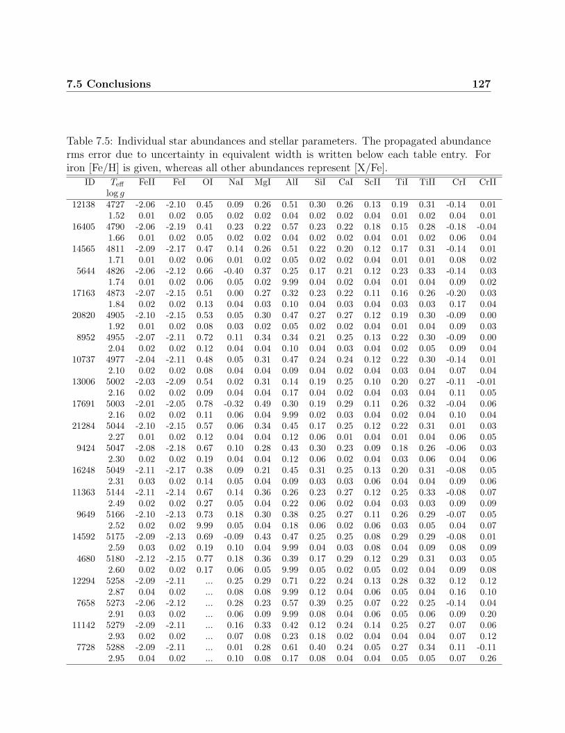
7.5 Conclusions 127
Table 7.5: Individual star abundances and stellar parameters. The propagated abundancerms error due to uncertainty in equivalent width is written below each table entry. Foriron [Fe/H] is given, whereas all other abundances represent [X/Fe].
ID Teff FeII FeI OI NaI MgI AlI SiI CaI ScII TiI TiII CrI CrIIlog g
12138 4727 -2.06 -2.10 0.45 0.09 0.26 0.51 0.30 0.26 0.13 0.19 0.31 -0.14 0.011.52 0.01 0.02 0.05 0.02 0.02 0.04 0.02 0.02 0.04 0.01 0.02 0.04 0.01
16405 4790 -2.06 -2.19 0.41 0.23 0.22 0.57 0.23 0.22 0.18 0.15 0.28 -0.18 -0.041.66 0.01 0.02 0.05 0.02 0.02 0.04 0.02 0.02 0.04 0.01 0.02 0.06 0.04
14565 4811 -2.09 -2.17 0.47 0.14 0.26 0.51 0.22 0.20 0.12 0.17 0.31 -0.14 0.011.71 0.01 0.02 0.06 0.01 0.02 0.05 0.02 0.02 0.04 0.01 0.01 0.08 0.02
5644 4826 -2.06 -2.12 0.66 -0.40 0.37 0.25 0.17 0.21 0.12 0.23 0.33 -0.14 0.031.74 0.01 0.02 0.06 0.05 0.02 9.99 0.04 0.02 0.04 0.01 0.04 0.09 0.02
17163 4873 -2.07 -2.15 0.51 0.00 0.27 0.32 0.23 0.22 0.11 0.16 0.26 -0.20 0.031.84 0.02 0.02 0.13 0.04 0.03 0.10 0.04 0.03 0.04 0.03 0.03 0.17 0.04
20820 4905 -2.10 -2.15 0.53 0.05 0.30 0.47 0.27 0.27 0.12 0.19 0.30 -0.09 0.001.92 0.01 0.02 0.08 0.03 0.02 0.05 0.02 0.02 0.04 0.01 0.04 0.09 0.03
8952 4955 -2.07 -2.11 0.72 0.11 0.34 0.34 0.21 0.25 0.13 0.22 0.30 -0.09 0.002.04 0.02 0.02 0.12 0.04 0.04 0.10 0.04 0.03 0.04 0.02 0.05 0.09 0.04
10737 4977 -2.04 -2.11 0.48 0.05 0.31 0.47 0.24 0.24 0.12 0.22 0.30 -0.14 0.012.10 0.02 0.02 0.08 0.04 0.04 0.09 0.04 0.02 0.04 0.03 0.04 0.07 0.04
13006 5002 -2.03 -2.09 0.54 0.02 0.31 0.14 0.19 0.25 0.10 0.20 0.27 -0.11 -0.012.16 0.02 0.02 0.09 0.04 0.04 0.17 0.04 0.02 0.04 0.03 0.04 0.11 0.05
17691 5003 -2.01 -2.05 0.78 -0.32 0.49 0.30 0.19 0.29 0.11 0.26 0.32 -0.04 0.062.16 0.02 0.02 0.11 0.06 0.04 9.99 0.02 0.03 0.04 0.02 0.04 0.10 0.04
21284 5044 -2.10 -2.15 0.57 0.06 0.34 0.45 0.17 0.25 0.12 0.22 0.31 0.01 0.032.27 0.01 0.02 0.12 0.04 0.04 0.12 0.06 0.01 0.04 0.01 0.04 0.06 0.05
9424 5047 -2.08 -2.18 0.67 0.10 0.28 0.43 0.30 0.23 0.09 0.18 0.26 -0.06 0.032.30 0.02 0.02 0.19 0.04 0.04 0.12 0.06 0.02 0.04 0.03 0.06 0.04 0.06
16248 5049 -2.11 -2.17 0.38 0.09 0.21 0.45 0.31 0.25 0.13 0.20 0.31 -0.08 0.052.31 0.03 0.02 0.14 0.05 0.04 0.09 0.03 0.03 0.06 0.04 0.04 0.09 0.06
11363 5144 -2.11 -2.14 0.67 0.14 0.36 0.26 0.23 0.27 0.12 0.25 0.33 -0.08 0.072.49 0.02 0.02 0.27 0.05 0.04 0.22 0.06 0.02 0.04 0.03 0.03 0.09 0.09
9649 5166 -2.10 -2.13 0.73 0.18 0.30 0.38 0.25 0.27 0.11 0.26 0.29 -0.07 0.052.52 0.02 0.02 9.99 0.05 0.04 0.18 0.06 0.02 0.06 0.03 0.05 0.04 0.07
14592 5175 -2.09 -2.13 0.69 -0.09 0.43 0.47 0.25 0.25 0.08 0.29 0.29 -0.08 0.012.59 0.03 0.02 0.19 0.10 0.04 9.99 0.04 0.03 0.08 0.04 0.09 0.08 0.09
4680 5180 -2.12 -2.15 0.77 0.18 0.36 0.39 0.17 0.29 0.12 0.29 0.31 0.03 0.052.60 0.02 0.02 0.17 0.06 0.05 9.99 0.05 0.02 0.05 0.02 0.04 0.09 0.08
12294 5258 -2.09 -2.11 ... 0.25 0.29 0.71 0.22 0.24 0.13 0.28 0.32 0.12 0.122.87 0.04 0.02 ... 0.08 0.08 9.99 0.12 0.04 0.06 0.05 0.04 0.16 0.10
7658 5273 -2.06 -2.12 ... 0.28 0.23 0.57 0.39 0.25 0.07 0.22 0.25 -0.14 0.042.91 0.03 0.02 ... 0.06 0.09 9.99 0.08 0.04 0.06 0.05 0.06 0.09 0.20
11142 5279 -2.09 -2.11 ... 0.16 0.33 0.42 0.12 0.24 0.14 0.25 0.27 0.07 0.062.93 0.02 0.02 ... 0.07 0.08 0.23 0.18 0.02 0.04 0.04 0.04 0.07 0.12
7728 5288 -2.09 -2.11 ... 0.01 0.28 0.61 0.40 0.24 0.05 0.27 0.34 0.11 -0.112.95 0.04 0.02 ... 0.10 0.08 0.17 0.08 0.04 0.04 0.05 0.05 0.07 0.26
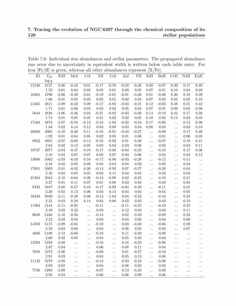
1287. Tracing the evolution of NGC 6397 through the chemical composition of its
stellar populations
Table 7.6: Individual star abundances and stellar parameters. The propagated abundancerms error due to uncertainty in equivalent width is written below each table entry. Foriron [Fe/H] is given, whereas all other abundances represent [X/Fe].
ID Teff FeII MnI CoI NiI CuI ZnI YII ZrII BaII CeII NdII EuIIlog g
12138 4727 -2.06 -0.43 0.01 -0.17 -0.76 -0.02 -0.26 0.09 -0.07 0.39 0.17 0.491.52 0.01 0.04 0.02 0.02 0.01 0.09 0.05 0.07 0.01 0.10 0.04 0.03
16405 4790 -2.06 -0.49 0.01 -0.19 -0.81 -0.01 -0.26 0.01 -0.06 0.40 0.18 0.391.66 0.01 0.05 0.03 0.02 0.01 0.02 0.04 0.07 0.02 0.02 0.02 0.10
14565 4811 -2.09 -0.50 0.09 -0.17 -0.82 -0.03 -0.21 0.12 -0.03 0.48 0.21 0.421.71 0.01 0.06 0.02 0.02 0.03 0.05 0.04 0.07 0.01 0.08 0.03 0.08
5644 4826 -2.06 -0.36 0.04 -0.21 -0.82 -0.03 -0.30 0.14 -0.10 0.42 0.17 0.381.74 0.01 0.05 0.05 0.01 0.02 0.02 0.05 0.10 0.02 0.14 0.03 0.05
17163 4873 -2.07 -0.58 -0.12 -0.18 -1.03 -0.02 -0.24 0.17 -0.06 ... 0.12 0.301.84 0.02 0.14 0.12 0.04 0.09 0.03 0.04 0.08 0.03 ... 0.03 0.18
20820 4905 -2.10 -0.40 0.11 -0.16 -0.91 -0.04 -0.27 ... -0.09 ... 0.17 0.491.92 0.01 0.04 0.05 0.02 0.05 0.01 0.06 ... 0.01 ... 0.06 0.05
8952 4955 -2.07 -0.60 0.14 -0.16 -0.92 0.01 -0.30 ... -0.07 ... 0.19 0.412.04 0.02 0.12 0.05 0.03 0.04 0.03 0.06 ... 0.02 ... 0.03 0.11
10737 4977 -2.04 -0.47 0.19 -0.17 -0.88 -0.04 -0.25 ... -0.10 ... 0.17 0.362.10 0.02 0.07 0.07 0.03 0.07 0.03 0.06 ... 0.02 ... 0.04 0.12
13006 5002 -2.03 -0.43 0.16 -0.17 -0.80 -0.03 -0.28 ... -0.12 ... 0.11 ...2.16 0.02 0.05 0.08 0.04 0.04 0.04 0.02 ... 0.03 ... 0.04 ...
17691 5003 -2.01 -0.42 0.20 -0.14 -0.92 0.07 -0.27 ... -0.20 ... 0.04 ...2.16 0.02 0.05 0.05 0.03 0.11 0.04 0.05 ... 0.03 ... 0.03 ...
21284 5044 -2.10 -0.64 0.26 -0.13 -0.98 0.02 -0.25 ... -0.10 ... 0.21 ...2.27 0.01 0.11 0.07 0.01 0.08 0.03 0.04 ... 0.02 ... 0.05 ...
9424 5047 -2.08 -0.57 0.10 -0.17 -0.92 -0.04 -0.29 ... -0.11 ... 0.21 ...2.30 0.02 0.13 0.06 0.03 0.14 0.04 0.02 ... 0.04 ... 0.05 ...
16248 5049 -2.11 -0.49 0.06 -0.12 -1.04 0.04 -0.23 ... -0.10 ... 0.25 ...2.31 0.03 0.20 0.14 0.04 0.08 0.03 0.03 ... 0.03 ... 0.10 ...
11363 5144 -2.11 -0.92 ... -0.11 ... -0.11 -0.25 ... -0.10 ... 0.22 ...2.49 0.02 0.22 ... 0.03 ... 0.12 0.04 ... 0.03 ... 0.11 ...
9649 5166 -2.10 -0.56 ... -0.14 ... 0.02 -0.29 ... -0.09 ... 0.23 ...2.52 0.02 0.04 ... 0.04 ... 0.04 0.02 ... 0.04 ... 0.09 ...
14592 5175 -2.09 -0.65 ... -0.10 ... 0.03 -0.30 ... -0.06 ... 0.20 ...2.59 0.03 0.08 ... 0.04 ... 0.06 0.05 ... 0.03 ... 0.07 ...
4680 5180 -2.12 -0.60 ... -0.10 ... 0.11 -0.20 ... -0.08 ... ... ...2.60 0.02 0.05 ... 0.04 ... 0.05 0.03 ... 0.04 ... ... ...
12294 5258 -2.09 ... ... -0.16 ... 0.16 -0.23 ... -0.06 ... ... ...2.87 0.04 ... ... 0.06 ... 0.08 0.11 ... 0.04 ... ... ...
7658 5273 -2.06 ... ... -0.09 ... 0.01 -0.27 ... -0.10 ... ... ...2.91 0.03 ... ... 0.04 ... 0.05 0.13 ... 0.06 ... ... ...
11142 5279 -2.09 ... ... -0.13 ... 0.03 -0.22 ... -0.06 ... ... ...2.93 0.02 ... ... 0.04 ... 0.06 0.02 ... 0.03 ... ... ...
7728 5288 -2.09 ... ... -0.07 ... 0.13 -0.23 ... 0.06 ... ... ...2.95 0.04 ... ... 0.06 ... 0.06 0.09 ... 0.06 ... ... ...

Chapter 8
Conclusions and outlook
It is beyond doubt that high-precision abundance analysis is a powerful tool to investigatethe origin and cosmic evolution of elements and the nature of the stars in which they arecreated, destroyed and re-cycled. The work presented in this thesis has shed new light onthe processes that affect the evolution of Li abundance in low-mass stars, which in turn canhelp us form a consistent picture of primordial nucleosynthesis and the birth of the Universe.We have also been able to trace the star formation history that characterise globularclusters, which are fundamental building blocks of the Milky-Way and other galaxies.
8.1 The cosmological Li problem
Our detailed analysis of the Li surface abundances of globular cluster stars certainly sup-ports the hypothesis that some Li has settled below the convection zone in metal-poormain sequence stars and is being dredged up to the surface in the early subgiant phase.As discussed in Chapter 6, this scenario may provide at least part of the solution to thecosmological lithium dilemma. Encouraging in this context is the good consistency foundfor the abundance trends of other elements, like Ca and Na, as presented in this thesis andadditionally Fe, Mg, and Ti, as shown in Lind et al. (2008); Korn et al. (2007).
However, given the subtle effects that atomic diffusion has on the surface evolutionof Li and other elements, it will require much effort both on the modelling side and theobservational side to convincingly resolve the cosmological Li problem. Future observationsmust map the metallicity dependence of the depletion physics in order to constrain theelusive source of turbulence in radiative layers. Globular clusters are excellent targetsfor such investigations due to their uniform ages and metallicities, and the large numberstatistics that can be obtained. In addition, the poorly investigated relation between Liabundance and stellar rotation and/or binarity could give important insights. Rotatingstellar models with a consistent physical treatment of the transport of angular momentumand chemicals (Talon & Charbonnel, 2003, 2004) should be extended to Pop II stars, so thatpredictions for the surface evolution of elements can be made directly from first principles.
Should we finally reach a consensus between observations of 7Li in metal-poor halo
130 8. Conclusions and outlook
stars and modelling of the microscopic diffusion of this element, we may simultaneouslyexacerbate another alarming cosmological problem. The handful of measurements thathave been made of the much more fragile isotope 6Li (Asplund et al., 2006; Cayrel et al.,2007; Smith et al., 1998), will namely be exceedingly difficult to explain if 7Li has under-gone significant surface depletion, given that 6Li is not synthesised in the standard BigBang scenario. Clearly, the 6Li abundances deserve further attention, especially consider-ing the challenges involved in its measurements. The lighter isotope, if present, can onlybe detected through a slight depression in the red wing of Li I 670.7 nm line. To properlydisentangle the 6Li feature from asymmetries caused by the convective motions requiresprecise 3D modelling accounting for departures from LTE, as well as high-quality observa-tional data. The sampling of the necessary extremely high-resolution spectra will certainlybecome more routinely performed with future large telescope facilities, like the ultra-stableoptical spectrograph ESPRESSO planned for the VLT (Pasquini et al., 2009), or CODEX(R <∼ 120000) proposed for the E-ELT (Pasquini et al., 2010).
In addition to the debate on the amount of photospheric depletion of Li in stars, thisfundamental discrepancy has many other interesting aspects. Maybe the Spite plateau isindeed representative of the primordial abundance, but the standard model of Big Bangnucleosynthesis is in error, despite its numerous successes. Various flavours of non-standardphysics like decaying dark matter particles at the time of BBN, have been suggested toreconcile both or either of the 7Li and 6Li abundances with the predictions (e.g. Jedamzik &Pospelov 2009, and references therein). The Large Hadron Collider may in the coming yearsbring discoveries of supersymmetry and thereby support or refute the proposed particles.
8.2 Multiple populations in globular clusters
Our work has made a convincing case for the presence of two stellar populations in theglobular cluster NGC6397. With a high-precision, homogeneous analysis of a large stellarsample we could disentangle differences in the original chemical compositions of stars withevolutionary effects, causing elemental abundances differences between stars in differentregions of the HR diagram. The robust signs of intrinsic bimodality in spectroscopic Na andphotometric N abundances are promising for the ability of future studies to unequivocallyseparate the different populations and pin-point the differences in the chemical abundancesof many more elements to high precision.
The intriguing question of the nature of the early generation of polluting stars in glob-ular cluster has indeed great potential of being resolved within the coming decade or so.Several different observational tests can and should be made is this direction, like exam-ining the C+N+O abundance spectroscopically for a large sample of stars belonging todifferent generations in a globular cluster, as this sum is predicted to increase with AGBstar pollution. Investigations have so far reached different conclusions on this point fordifferent clusters (e.g. Yong et al. 2009; Smith et al. 2005). Also the Li abundances of theextreme populations in clusters like NGC2808, could give a more decisive answer, sincesuper-AGB stars may under certain circumstances be efficient Li-producers (Ventura &
8.3 The future of high-precision abundance analysis 131
D’Antona, 2010), whereas massive stars only destroy this element. Additionally, it is defi-nitely worthwhile to extend the work presented in Sect. 7.3.5 to cluster having undergoneheavier pollution than NGC6397, and constrain spectroscopically the helium difference ofstellar ’pairs’ belonging to different generations. It is possible, that ∆Y can even be in-ferred directly by targeting the chromospheric He I line at 1083 nm in red giants, providedthat a reliable non-LTE analysis technique can be developed (which is an extremely chal-lenging task). From the stellar modelling point-of-view the credibility of AGB star yieldswould surely benefit from improvements in the treatment of convection, and mass losswhich contain the largest uncertainties (Charbonnel, 2005; Ventura & D’Antona, 2010).
Present day medium-to-high resolution spectrographs on the generation of very largetelescopes are operating at the limit of their capabilities when targeting turn-off stars evenin nearby globular clusters. However, the next generation of extremely large telescopes willcertainly provide much greater feasibility and enable us to probe both farther and deeper.The optical and near infra-red multi-object spectrograph OPTIMUS-EVE proposed forthe E-ELT (Hammer et al., 2010) will be able to collect light from 40-70 objects with aresolving power of R = 18000 − 30000, but vastly superior in terms of efficiency with its42m mirror (target depth for R = 20000− 30000 observations is I = 23.5).
8.3 The future of high-precision abundance analysis
The non-LTE analysis presented in Chapter 2 has already contributed to a more accuratederivation of Li abundances in late-type stars for a variety of different applications, suchas the modelling of the Spite Plateau of halo stars (Melendez et al., 2010), the connectionbetween stellar Li abundance and the existence of orbiting exo-planets (Baumann et al.,2010), and the origin of the Li-enrichment that has been detected in some giant stars(Kumar & Reddy, 2009; Gonzalez et al., 2009). Especially in the latter case, the non-LTEcorrections can be size-able (<∼ +0.35 dex) due to efficient over-ionisation in low surface-gravity stars (see Sect. 3.3) and thus crucial for correct interpretations.
Surely, future Na abundance analyses can benefit in a similar manner from the resultspresented in Chapter 3. By establishing the most realistic Na model atom to date, wehave been able to clarify the influence from remaining uncertainties in collisional cross-sections, and thereby ensured that the non-LTE modelling is indeed robust in this respectand certainly always a better approach than traditional LTE modelling. Further, ourinitial attempts to extend the non-LTE analysis for trace elements to 3D hydro-dynamicalmodel atmospheres are indeed encouraging. We have demonstrated that we are able toaccurately predict solar line profiles in 3D without the introduction of fudge factors suchas micro- and macroturbulence and make a precise derivation of the solar Na abundance.The centre-to-limb variations of the solar Na I lines are not reproduced to a satisfactorydegree however, which calls for further improvements of the modelling procedure beforecombined 3D, non-LTE modelling can be extended to a cover a wider stellar parameterspace.
Nevertheless, 3D modelling of late-type stellar atmospheres bears enormous potential
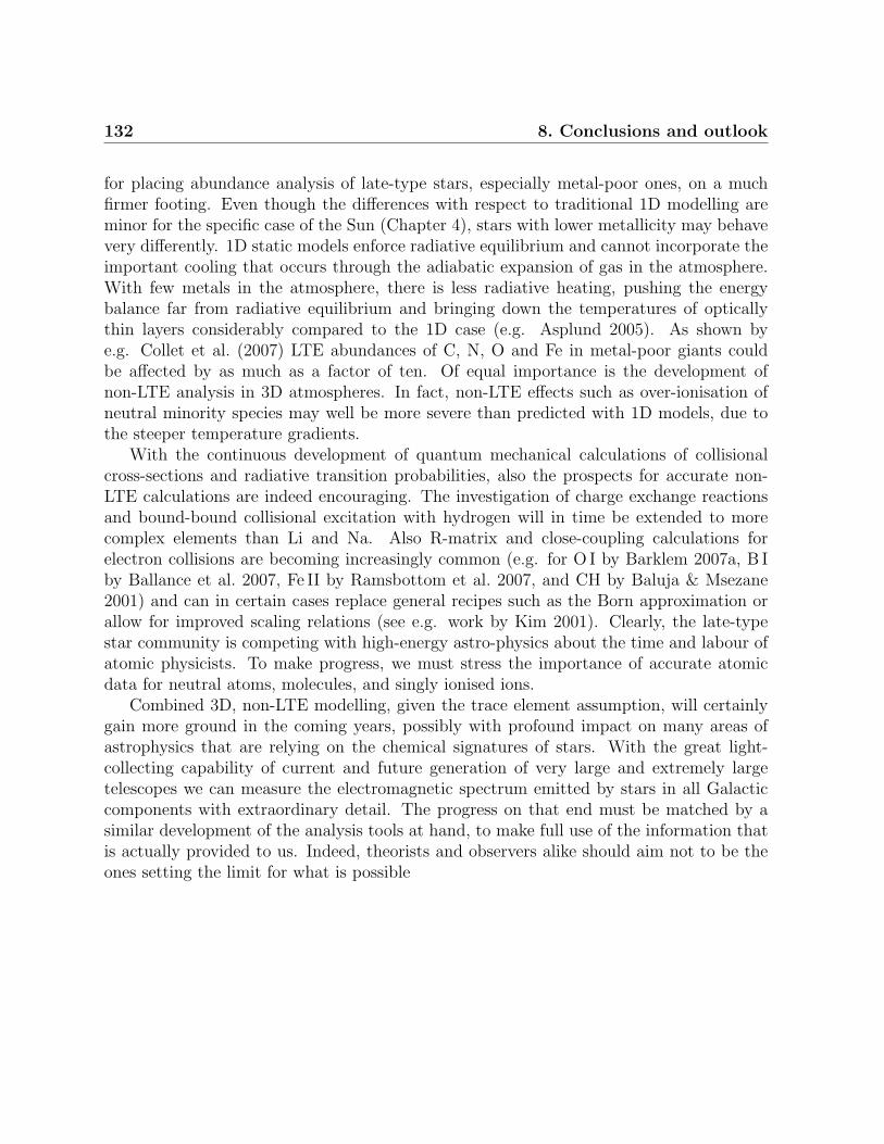
132 8. Conclusions and outlook
for placing abundance analysis of late-type stars, especially metal-poor ones, on a muchfirmer footing. Even though the differences with respect to traditional 1D modelling areminor for the specific case of the Sun (Chapter 4), stars with lower metallicity may behavevery differently. 1D static models enforce radiative equilibrium and cannot incorporate theimportant cooling that occurs through the adiabatic expansion of gas in the atmosphere.With few metals in the atmosphere, there is less radiative heating, pushing the energybalance far from radiative equilibrium and bringing down the temperatures of opticallythin layers considerably compared to the 1D case (e.g. Asplund 2005). As shown bye.g. Collet et al. (2007) LTE abundances of C, N, O and Fe in metal-poor giants couldbe affected by as much as a factor of ten. Of equal importance is the development ofnon-LTE analysis in 3D atmospheres. In fact, non-LTE effects such as over-ionisation ofneutral minority species may well be more severe than predicted with 1D models, due tothe steeper temperature gradients.
With the continuous development of quantum mechanical calculations of collisionalcross-sections and radiative transition probabilities, also the prospects for accurate non-LTE calculations are indeed encouraging. The investigation of charge exchange reactionsand bound-bound collisional excitation with hydrogen will in time be extended to morecomplex elements than Li and Na. Also R-matrix and close-coupling calculations forelectron collisions are becoming increasingly common (e.g. for O I by Barklem 2007a, B Iby Ballance et al. 2007, Fe II by Ramsbottom et al. 2007, and CH by Baluja & Msezane2001) and can in certain cases replace general recipes such as the Born approximation orallow for improved scaling relations (see e.g. work by Kim 2001). Clearly, the late-typestar community is competing with high-energy astro-physics about the time and labour ofatomic physicists. To make progress, we must stress the importance of accurate atomicdata for neutral atoms, molecules, and singly ionised ions.
Combined 3D, non-LTE modelling, given the trace element assumption, will certainlygain more ground in the coming years, possibly with profound impact on many areas ofastrophysics that are relying on the chemical signatures of stars. With the great light-collecting capability of current and future generation of very large and extremely largetelescopes we can measure the electromagnetic spectrum emitted by stars in all Galacticcomponents with extraordinary detail. The progress on that end must be matched by asimilar development of the analysis tools at hand, to make full use of the information thatis actually provided to us. Indeed, theorists and observers alike should aim not to be theones setting the limit for what is possible
Bibliography
Allen, C. W. 1976, Astrophysical Quantities (Astrophysical Quantities, London: Athlone(3rd edition), 1976)
Allen, C. W. 2000, Allen’s Astrophysical Quantities, 4th edn. (Springer, Berlin)
Allende Prieto, C., Asplund, M., & Fabiani Bendicho, P. 2004, Astronomy and Astro-physics, 423, 1109
Allende Prieto, C., Hubeny, I., & Lambert, D. L. 2003, Astrophysical Journal, 591, 1192
Alonso, A., Arribas, S., & Martinez-Roger, C. 1996, Astronomy and Astrophysics, 313,873
Alonso, A., Arribas, S., & Martınez-Roger, C. 1999, Astronomy and Astrophysics, Supple-ment, 140, 261
Andrievsky, S. M., Spite, M., Korotin, S. A., et al. 2010, Astronomy and Astrophysics,509, A88+
Andrievsky, S. M., Spite, M., Korotin, S. A., et al. 2007, Astronomy and Astrophysics,464, 1081
Andrievsky, S. M., Spite, M., Korotin, S. A., et al. 2008, Astronomy and Astrophysics,481, 481
Anstee, S. D. & O’Mara, B. J. 1995, Monthly Notices of the Royal Astronomical Society,276, 859
Anthony-Twarog, B. J. & Twarog, B. A. 2000, Astronomical Journal, 120, 3111
Aoki, W., Barklem, P. S., Beers, T. C., et al. 2009, Astrophysical Journal, 698, 1803
Asplund, M. 2005, Annual Review of Astronomy and Astrophysics, 43, 481
Asplund, M., Carlsson, M., & Botnen, A. V. 2003, Astronomy and Astrophysics, 399, L31
Asplund, M., Grevesse, N., Sauval, A. J., & Scott, P. 2009, Annual Review of Astronomyand Astrophysics, 47, 481
134 BIBLIOGRAPHY
Asplund, M., Gustafsson, B., Kiselman, D., & Eriksson, K. 1997, Astronomy and Astro-physics, 318, 521
Asplund, M., Lambert, D. L., Nissen, P. E., Primas, F., & Smith, V. V. 2006, AstrophysicalJournal, 644, 229
Asplund, M. & Lind, K. 2010, in IAU Symposium, Vol. 268, IAU Symposium, ed. C. Char-bonnel, M. Tosi, F. Primas, & C. Chiappini, 191–200
Asplund, M., Nordlund, A., Trampedach, R., Allende Prieto, C., & Stein, R. F. 2000,Astronomy and Astrophysics, 359, 729
Asplund, M., Nordlund, A., Trampedach, R., & Stein, R. F. 1999, Astronomy and Astro-physics, 346, L17
Ballance, C. P., Griffin, D. C., Berrington, K. A., & Badnell, N. R. 2007, Journal of PhysicsB Atomic Molecular Physics, 40, 1131
Baluja, K. L. & Msezane, A. Z. 2001, Journal of Physics B Atomic Molecular Physics, 34,3157
Barklem, P. S. 2007a, Astronomy and Astrophysics, 462, 781
Barklem, P. S. 2007b, Astronomy and Astrophysics, 466, 327
Barklem, P. S., Belyaev, A. K., & Asplund, M. 2003, Astronomy and Astrophysics, 409,L1
Barklem, P. S., Belyaev, A. K., Dickinson, A. S., & Gadea, F. X. 2010, Astronomy andAstrophysics, 519, A20+
Barklem, P. S., Christlieb, N., Beers, T. C., et al. 2005, Astronomy and Astrophysics, 439,129
Barklem, P. S. & O’Mara, B. J. 1997, Monthly Notices of the Royal Astronomical Society,290, 102
Barklem, P. S., Piskunov, N., & O’Mara, B. J. 2000, Astronomy and Astrophysics, 363,1091
Baumann, P., Ramırez, I., Melendez, J., Asplund, M., & Lind, K. 2010, Astronomy andAstrophysics, 519, A87+
Bell, R. A., Dickens, R. J., & Gustafsson, B. 1979, Astrophysical Journal, 229, 604
Belyaev, A. K. & Barklem, P. S. 2003, Physical Review A: General Physics, 68, 062703
Bensby, T., Feltzing, S., & Lundstrom, I. 2003, Astronomy and Astrophysics, 410, 527
BIBLIOGRAPHY 135
Bergemann, M. & Gehren, T. 2008, Astronomy and Astrophysics, 492, 823
Bielski, A. 1975, Journal of Quantitative Spectroscopy and Radiative Transfer, 15, 463
Biemont, E., Baudoux, M., Kurucz, R. L., Ansbacher, W., & Pinnington, E. H. 1991,Astronomy and Astrophysics, 249, 539
Biemont, E. & Zeippen, C. J. 1992, Astronomy and Astrophysics, 265, 850
Bonifacio, P., Molaro, P., Sivarani, T., et al. 2007a, Astronomy and Astrophysics, 462, 851
Bonifacio, P., Pasquini, L., Molaro, P., et al. 2007b, Astronomy and Astrophysics, 470, 153
Bonifacio, P., Pasquini, L., Spite, F., et al. 2002, Astronomy and Astrophysics, 390, 91
Botnen, A. 1997, Master’s thesis, Master’s thesis, Inst. Theor. Astrophys. Oslo (1997)
Briley, M. M., Bell, R. A., Hoban, S., & Dickens, R. J. 1990, Astrophysical Journal, 359,307
Brodie, J. P. & Strader, J. 2006, Annual Review of Astronomy and Astrophysics, 44, 193
Bruls, J. H. M. J., Rutten, R. J., & Shchukina, N. G. 1992, Astronomy and Astrophysics,265, 237
Burris, D. L., Pilachowski, C. A., Armandroff, T. E., et al. 2000, Astrophysical Journal,544, 302
Carlson, B. G. 1963, Methods of Computational Physics, ed. Alder, B., Fernbach, S.,Rottenberg, M (Academic Press, New York)
Carlsson, M. 1986, Uppsala Astronomical Observatory Reports, 33
Carlsson, M. 1992, in Astronomical Society of the Pacific Conference Series, Vol. 26, CoolStars, Stellar Systems, and the Sun, ed. M. S. Giampapa & J. A. Bookbinder, 499–+
Carlsson, M., Rutten, R. J., Bruls, J. H. M. J., & Shchukina, N. G. 1994, Astronomy andAstrophysics, 288, 860
Carretta, E., Bragaglia, A., Gratton, R., & Lucatello, S. 2009a, Astronomy and Astro-physics, 505, 139
Carretta, E., Bragaglia, A., Gratton, R. G., et al. 2009b, Astronomy and Astrophysics,505, 117
Carretta, E., Bragaglia, A., Gratton, R. G., et al. 2010, Astronomy and Astrophysics, 516,A55+
136 BIBLIOGRAPHY
Carretta, E., Gratton, R. G., Lucatello, S., Bragaglia, A., & Bonifacio, P. 2005, Astronomyand Astrophysics, 433, 597
Casagrande, L., Ramırez, I., Melendez, J., Bessell, M., & Asplund, M. 2010, Astronomyand Astrophysics, 512, A54+
Castelli, F. & Kurucz, R. L. 2004, ArXiv Astrophysics e-prints
Castilho, B. V., Pasquini, L., Allen, D. M., Barbuy, B., & Molaro, P. 2000, Astronomyand Astrophysics, 361, 92
Cayrel, R., Depagne, E., Spite, M., et al. 2004, Astronomy and Astrophysics, 416, 1117
Cayrel, R., Steffen, M., Chand, H., et al. 2007, Astronomy and Astrophysics, 473, L37
Charbonnel, C. 2005, in IAU Symposium, Vol. 228, From Lithium to Uranium: ElementalTracers of Early Cosmic Evolution, ed. V. Hill, P. Francois, & F. Primas, 347–356
Charbonnel, C. 2007, in Astronomical Society of the Pacific Conference Series, Vol. 378,Why Galaxies Care About AGB Stars: Their Importance as Actors and Probes, ed.F. Kerschbaum, C. Charbonnel, & R. F. Wing, 416–+
Charbonnel, C. & Lagarde, N. 2010, Astronomy and Astrophysics, 522, A10+
Charbonnel, C. & Primas, F. 2005, Astronomy and Astrophysics, 442, 961
Charbonnel, C. & Talon, S. 2005, Science, 309, 2189
Charbonnel, C. & Talon, S. 2008, in IAU Symposium, Vol. 252, IAU Symposium, ed.L. Deng & K. L. Chan, 163–174
Charbonnel, C. & Zahn, J.-P. 2007, Astronomy and Astrophysics, 467, L15
Collet, R., Asplund, M., & Trampedach, R. 2007, Astronomy and Astrophysics, 469, 687
Crawford, D. L. 1975, Publications of the Astronomical Society of the Pacific, 87, 481
Croft, H., Dickinson, A. S., & Gadea, F. X. 1999, Monthly Notices of the Royal Astronom-ical Society, 304, 327
Cyburt, R. H., Fields, B. D., & Olive, K. A. 2008, Journal of Cosmology and Astro-ParticlePhysics, 11, 12
D’Antona, F. & Caloi, V. 2008, Monthly Notices of the Royal Astronomical Society, 390,693
de Mink, S. E., Pols, O. R., Langer, N., & Izzard, R. G. 2009, Astronomy and Astrophysics,507, L1
BIBLIOGRAPHY 137
Decressin, T., Baumgardt, H., Charbonnel, C., & Kroupa, P. 2010, Astronomy and Astro-physics, 516, A73+
Decressin, T., Charbonnel, C., & Meynet, G. 2007a, Astronomy and Astrophysics, 475,859
Decressin, T., Charbonnel, C., Siess, L., et al. 2009, Astronomy and Astrophysics, 505, 727
Decressin, T., Meynet, G., Charbonnel, C., Prantzos, N., & Ekstrom, S. 2007b, Astronomyand Astrophysics, 464, 1029
Dekker, H., D’Odorico, S., Kaufer, A., Delabre, B., & Kotzlowski, H. 2000, in Society ofPhoto-Optical Instrumentation Engineers (SPIE) Conference Series, Vol. 4008, Societyof Photo-Optical Instrumentation Engineers (SPIE) Conference Series, ed. M. Iye &A. F. Moorwood, 534–545
Denisenkov, P. A. & Denisenkova, S. N. 1989, Astronomicheskij Tsirkulyar, 1538, 11
Denisenkov, P. A. & Denisenkova, S. N. 1990, Soviet Astronomy Letters, 16, 275
di Criscienzo, M., D’Antona, F., & Ventura, P. 2010, Astronomy and Astrophysics, 511,A70+
Dimitrijevic, M. S. & Sahal-Brechot, S. 1985, Journal of Quantitative Spectroscopy andRadiative Transfer, 34, 149
Dimitrijevic, M. S. & Sahal-Brechot, S. 1990, Journal of Quantitative Spectroscopy andRadiative Transfer, 44, 421
D’Orazi, V., Lucatello, S., Gratton, R., et al. 2010, Astrophysical Journal, Letters, 713, L1
Drawin, H.-W. 1968, Zeitschrift fur Physik, 211, 404
Dunkley, J., Komatsu, E., Nolta, M. R., et al. 2009, Astrophysical Journal, Supplement,180, 306
Edvardsson, B., Andersen, J., Gustafsson, B., et al. 1993, Astronomy and Astrophysics,275, 101
Ekstrom, S., Meynet, G., Maeder, A., & Barblan, F. 2008, Astronomy and Astrophysics,478, 467
Fabbian, D., Asplund, M., Barklem, P. S., Carlsson, M., & Kiselman, D. 2009, Astronomyand Astrophysics, 500, 1221
Feautrier, N., Han, X.-Y., & Lind, K. in preparation, Astronomy and Astrophysics
Francois, P., Depagne, E., Hill, V., et al. 2007, Astronomy and Astrophysics, 476, 935
138 BIBLIOGRAPHY
Freytag, B., Allard, F., Ludwig, H., Homeier, D., & Steffen, M. 2010, Astronomy andAstrophysics, 513, A19+
Fuhr, J. R., Martin, G. A., & Wiese, W. L. 1988, Atomic transition probabilities. Scandiumthrough Manganese (New York: American Institute of Physics (AIP) and AmericanChemical Society, 1988)
Fuhrmann, K., Pfeiffer, M., Frank, C., Reetz, J., & Gehren, T. 1997, Astronomy andAstrophysics, 323, 909
Gao, X., Han, X., Voky, L., Feautrier, N., & Li, J. 2010, Physical Review A: GeneralPhysics, 81, 022703
Gehren, T., Shi, J. R., Zhang, H. W., Zhao, G., & Korn, A. J. 2006, Astronomy andAstrophysics, 451, 1065
Gonzalez, O. A., Zoccali, M., Monaco, L., et al. 2009, Astronomy and Astrophysics, 508,289
Gratton, R., Sneden, C., & Carretta, E. 2004, Annual Review of Astronomy and Astro-physics, 42, 385
Gratton, R. G., Bonifacio, P., Bragaglia, A., et al. 2001, Astronomy and Astrophysics, 369,87
Gratton, R. G., Carretta, E., Claudi, R., Lucatello, S., & Barbieri, M. 2003, Astronomyand Astrophysics, 404, 187
Gratton, R. G., Sneden, C., Carretta, E., & Bragaglia, A. 2000, Astronomy and Astro-physics, 354, 169
Gray, D. F. 2005, The Observation and Analysis of Stellar Photospheres (Cambridge Uni-versity Press, 3rd ed.)
Grevesse, N., Asplund, M., & Sauval, A. J. 2007, Space Science Reviews, 130, 105
Grundahl, F., Briley, M., Nissen, P. E., & Feltzing, S. 2002a, Astronomy and Astrophysics,385, L14
Grundahl, F., Catelan, M., Landsman, W. B., Stetson, P. B., & Andersen, M. I. 1999,Astrophysical Journal, 524, 242
Grundahl, F., Stetson, P. B., & Andersen, M. I. 2002b, Astronomy and Astrophysics, 395,481
Grundahl, F., Vandenberg, D. A., & Andersen, M. I. 1998, Astrophysical Journal, Letters,500, L179+
BIBLIOGRAPHY 139
Grundahl, F., VandenBerg, D. A., Bell, R. A., Andersen, M. I., & Stetson, P. B. 2000,Astronomical Journal, 120, 1884
Gustafsson, B., Bell, R. A., Eriksson, K., & Nordlund, A. 1975, Astronomy and Astro-physics, 42, 407
Gustafsson, B., Edvardsson, B., Eriksson, K., et al. 2008, Astronomy and Astrophysics,486, 951
Hammer, F., Kaper, L., & Dalton, G. 2010, The Messenger, 140, 36
Hannaford, P., Lowe, R. M., Grevesse, N., Biemont, E., & Whaling, W. 1982, AstrophysicalJournal, 261, 736
Harris, W. E. 1996, Astronomical Journal, 112, 1487
Hauschildt, P. H., Allard, F., & Baron, E. 1999, Astrophysical Journal, 512, 377
Hayek, W., Asplund, M., Collet, R., & Nordlund, A. submitted, Astronomy and Astro-physics
Hoang Binh, D. & Van Regemorter, H. 1997, Journal of Physics B Atomic MolecularPhysics, 30, 2403
Holweger, H. & Mueller, E. A. 1974, Solar Physics, 39, 19
Hosford, A., Ryan, S. G., Garcıa Perez, A. E., Norris, J. E., & Olive, K. A. 2009, Astronomyand Astrophysics, 493, 601
Igenbergs, K., Schweinzer, J., Bray, I., Bridi, D., & Aumayr, F. 2008, Atomic Data andNuclear Data Tables, 94, 981
James, G., Francois, P., Bonifacio, P., et al. 2004, Astronomy and Astrophysics, 427, 825
Jedamzik, K. & Pospelov, M. 2009, New Journal of Physics, 11, 105028
Juric, M., Ivezic, Z., Brooks, A., et al. 2008, Astrophysical Journal, 673, 864
Kaulakys, B. 1991, Journal of Physics B Atomic Molecular Physics, 24, L127
Kelly, B. C. 2007, Astrophysical Journal, 665, 1489
Kim, Y. 2001, Physical Review A: General Physics, 64, 032713
Kiselman, D. 1997, Astrophysical Journal, Letters, 489, L107+
Kiselman, D. 2001, New Astronomy Review, 45, 559
Koch, A. & McWilliam, A. 2008, Astronomical Journal, 135, 1551

140 BIBLIOGRAPHY
Komarovskii, V. A. 1991, Optics and Spectroscopy, 71, 322
Korn, A. J., Grundahl, F., Richard, O., et al. 2006, Nature, 442, 657
Korn, A. J., Grundahl, F., Richard, O., et al. 2007, Astrophysical Journal, 671, 402
Krstic, P. S. & Schultz, D. R. 2009, Journal of Physics B Atomic Molecular Physics, 42,065207
Kumar, Y. B. & Reddy, B. E. 2009, Astrophysical Journal, Letters, 703, L46
Kurucz, R. L. 1970, SAO Special Report, 309
Kurucz, R. L. 1993, SYNTHE spectrum synthesis programs and line data (Kurucz CD-ROM, Cambridge, MA: Smithsonian Astrophysical Observatory, —c1993, December 4,1993)
Kurucz, R. L. & Peytremann, E. 1975, SAO Special Report, 362
Lambert, D. L. 1993, Physica Scripta Volume T, 47, 186
Langer, G. E., Hoffman, R., & Sneden, C. 1993, Publications of the Astronomical Societyof the Pacific, 105, 301
Lawler, J. E. & Dakin, J. T. 1989, Journal of the Optical Society of America B OpticalPhysics, 6, 1457
Lawler, J. E., Wickliffe, M. E., den Hartog, E. A., & Sneden, C. 2001, AstrophysicalJournal, 563, 1075
Leenaarts, J. & Carlsson, M. 2009, in Astronomical Society of the Pacific Conference Series,Vol. 415, Astronomical Society of the Pacific Conference Series, ed. B. Lites, M. Cheung,T. Magara, J. Mariska, & K. Reeves, 87–+
Lincke, R. & Ziegenbein, B. 1971, Zeitschrift fur Physik, 241, 369
Lind, K., Asplund, M., & Barklem, P. S. 2009a, Astronomy and Astrophysics, 503, 541
Lind, K., Asplund, M., Barklem, P. S., & Belyaev, A. K. submitteda, Astronomy andAstrophysics
Lind, K., Asplund, M., Barklem, P. S., Leenaarts, J., & Pereira, T. M. D. in preparation,Astronomy and Astrophysics
Lind, K., Charbonnel, C., Decressin, T., et al. submittedb, Astronomy and Astrophysics
Lind, K., Korn, A. J., Barklem, P. S., & Grundahl, F. 2008, Astronomy and Astrophysics,490, 777
BIBLIOGRAPHY 141
Lind, K., Primas, F., Charbonnel, C., Grundahl, F., & Asplund, M. 2009b, Astronomyand Astrophysics, 503, 545
Lindgard, A. & Nielson, S. E. 1977, Atomic Data and Nuclear Data Tables, 19, 533
Ljung, G., Nilsson, H., Asplund, M., & Johansson, S. 2006, Astronomy and Astrophysics,456, 1181
Ludwig, H., Caffau, E., Steffen, M., et al. 2009, Memorie della Societieta AstronomicaItalia, 80, 711
Martell, S. L. & Grebel, E. K. 2010, Astronomy and Astrophysics, 519, A14+
Martin, G. A., Fuhr, J. R., & Wiese, W. L. 1988, Phys. Chem. Ref. Data, 17, 3
Mashonkina, L. I., Shimanskii, V. V., & Sakhibullin, N. A. 2000, Astronomy Reports, 44,790
Melendez, J., Casagrande, L., Ramırez, I., Asplund, M., & Schuster, W. J. 2010, Astronomyand Astrophysics, 515, L3+
Melendez, J. & Ramırez, I. 2004, Astrophysical Journal, Letters, 615, L33
Meylan, G. & Heggie, D. C. 1997, Astronomy and Astrophysics Reviews, 8, 1
Michaud, G., Fontaine, G., & Beaudet, G. 1984, Astrophysical Journal, 282, 206
Mihalas, D. 1978, Stellar atmospheres (San Francisco, W. H. Freeman and Co. 2nd ed.)
Miles, B. M. & Wiese, W. L. 1969, Atomic Data, 1, 1
Milone, A. P., Piotto, G., King, I. R., et al. 2010, Astrophysical Journal, 709, 1183
Milone, A. P., Villanova, S., Bedin, L. R., et al. 2006, Astronomy and Astrophysics, 456,517
Muthsam, H. J., Kupka, F., Low-Baselli, B., et al. 2010, New Astronomy, 15, 460
Nieva, M. F. & Przybilla, N. 2007, Astronomy and Astrophysics, 467, 295
Nissen, P. E., Primas, F., Asplund, M., & Lambert, D. L. 2002, Astronomy and Astro-physics, 390, 235
Nissen, P. E. & Schuster, W. J. 2010, Astronomy and Astrophysics, 511, L10+
Nordlund, A., Stein, R. F., & Asplund, M. 2009, Living Reviews in Solar Physics, 6, 2
Norris, J. E. 2004, Astrophysical Journal, Letters, 612, L25
Norris, J. E. & Da Costa, G. S. 1995, Astrophysical Journal, Letters, 441, L81
142 BIBLIOGRAPHY
Norris, J. E., Ryan, S. G., & Beers, T. C. 2001, Astrophysical Journal, 561, 1034
O’Brian, T. R., Wickliffe, M. E., Lawler, J. E., Whaling, J. W., & Brault, W. 1991, Journalof the Optical Society of America B Optical Physics, 8, 1185
Onehag, A., Gustafsson, B., Eriksson, K., & Edvardsson, B. 2009, Astronomy and Astro-physics, 498, 527
Paresce, F. & De Marchi, G. 2000, Astrophysical Journal, 534, 870
Park, C. 1971, Journal of Quantitative Spectroscopy and Radiative Transfer, 11, 7
Pasquini, L., Avila, G., Blecha, A., et al. 2002, The Messenger, 110, 1
Pasquini, L., Bonifacio, P., Molaro, P., et al. 2005, Astronomy and Astrophysics, 441, 549
Pasquini, L., Bonifacio, P., Randich, S., Galli, D., & Gratton, R. G. 2004, Astronomy andAstrophysics, 426, 651
Pasquini, L., Cristiani, S., Garcia-Lopez, R., Haehnelt, M., & Mayor, M. 2010, The Mes-senger, 140, 20
Pasquini, L., Ecuvillon, A., Bonifacio, P., & Wolff, B. 2008, Astronomy and Astrophysics,489, 315
Pasquini, L., Manescau, A., Avila, G., et al. 2009, in Science with the VLT in the ELTEra, ed. A. Moorwood, 395–+
Pasquini, L. & Molaro, P. 1996, Astronomy and Astrophysics, 307, 761
Pavlenko, Y. V. & Magazzu, A. 1996, Astronomy and Astrophysics, 311, 961
Peach, G., Saraph, H. E., & Seaton, M. J. 1988, Journal of Physics B Atomic MolecularPhysics, 21, 3669
Pereira, T. M. D., Asplund, M., & Kiselman, D. 2009a, Astronomy and Astrophysics, 508,1403
Pereira, T. M. D., Asplund, M., Trampedach, R., Collet, R., & Leenaarts, J. submitted,Astronomy and Astrophysics
Pereira, T. M. D., Kiselman, D., & Asplund, M. 2009b, Astronomy and Astrophysics, 507,417
Phelps, J. O. & Lin, C. C. 1981, Physical Review A: General Physics, 24, 1299
Pickering, J. C., Thorne, A. P., & Perez, R. 2001, Astrophysical Journal, Supplement, 132,403

BIBLIOGRAPHY 143
Prantzos, N. & Charbonnel, C. 2006, Astronomy and Astrophysics, 458, 135
Prialnik, D. 2000, An Introduction to the Theory of Stellar Structure and Evolution, ed.Prialnik, D. (Cambridge University Press, 2000)
Primas, F. & Sobeck, J. 2008, in American Institute of Physics Conference Series, Vol.1001, Evolution and Nucleosynthesis in AGB Stars, ed. R. Guandalini, S. Palmerini, &M. Busso, 230–234
Pumo, M. L., D’Antona, F., & Ventura, P. 2008, Astrophysical Journal, Letters, 672, L25
Raassen, A. J. J. & Uylings, P. H. M. 1998, VizieR Online Data Catalog, 334, 300
Ramırez, I. & Melendez, J. 2005, Astrophysical Journal, 626, 465
Ramsbottom, C. A., Hudson, C. E., Norrington, P. H., & Scott, M. P. 2007, Astronomyand Astrophysics, 475, 765
Reddy, B. E., Tomkin, J., Lambert, D. L., & Allende Prieto, C. 2003, Monthly Notices ofthe Royal Astronomical Society, 340, 304
Reid, I. N. & Gizis, J. E. 1998, Astronomical Journal, 116, 2929
Richard, O., Michaud, G., & Richer, J. 2005, Astrophysical Journal, 619, 538
Richer, H. B., Dotter, A., Hurley, J., et al. 2008, Astronomical Journal, 135, 2141
Rutten, R. J. 2003, Radiative Transfer in Stellar Atmospheres (Utrecht University lecturenotes, 8th edition)
Ryan, S. G., Kajino, T., Beers, T. C., et al. 2001, Astrophysical Journal, 549, 55
Ryan, S. G., Norris, J. E., & Beers, T. C. 1999, Astrophysical Journal, 523, 654
Rybicki, G. B. & Hummer, D. G. 1991, Astronomy and Astrophysics, 245, 171
Sansonetti, C. J., Richou, B., Engleman, R. J., & Radziemski, L. J. 1995, Physical ReviewA: General Physics, 52, 2682
Sansonetti, J. E. 2008, Journal of Physical and Chemical Reference Data, 37, 1659
Scharmer, G. B., Bjelksjo, K., Korhonen, T. K., Lindberg, B., & Petterson, B. 2003,in Society of Photo-Optical Instrumentation Engineers (SPIE) Conference Series, Vol.4853, Society of Photo-Optical Instrumentation Engineers (SPIE) Conference Series, ed.S. L. Keil & S. V. Avakyan, 341–350
Scharmer, G. B. & Carlsson, M. 1985, Journal of Computational Physics, 59, 56
Seaton, M. J. 1962, Proceedings of the Physical Society, 79, 1105
144 BIBLIOGRAPHY
Shi, J. R., Gehren, T., & Zhao, G. 2004, Astronomy and Astrophysics, 423, 683
Shimanskaya, N. N., Mashonkina, L. I., & Sakhibullin, N. A. 2000, Astronomy Reports,44, 530
Short, C. I. & Hauschildt, P. H. 2003, Astrophysical Journal, 596, 501
Short, C. I. & Hauschildt, P. H. 2005, Astrophysical Journal, 618, 926
Smith, G. 1988, Journal of Physics B Atomic Molecular Physics, 21, 2827
Smith, G. & O’Neill, J. A. 1975, Astronomy and Astrophysics, 38, 1
Smith, G. & Raggett, D. S. J. 1981, Journal of Physics B Atomic Molecular Physics, 14,4015
Smith, V. V., Cunha, K., Ivans, I. I., et al. 2005, Astrophysical Journal, 633, 392
Smith, V. V., Lambert, D. L., & Nissen, P. E. 1998, Astrophysical Journal, 506, 405
Spite, M. & Spite, F. 1982, Nature, 297, 483
Stehle, C. & Hutcheon, R. 1999, Astronomy and Astrophysics, Supplement, 140, 93
Stein, R. F. & Nordlund, A. 1998, Astrophysical Journal, 499, 914
Stromgren, B., Gustafsson, B., & Olsen, E. H. 1982, Publications of the AstronomicalSociety of the Pacific, 94, 5
Sydoryk, I., Bezuglov, N. N., Beterov, I. I., et al. 2008, Physical Review A: General Physics,77, 042511
Takeda, Y. & Kawanomoto, S. 2005, Publications of the Astronomical Society of Japan,57, 45
Takeda, Y., Zhao, G., Takada-Hidai, M., et al. 2003, Chinese Journal of Astronomy andAstrophysics, 3, 316
Talon, S. & Charbonnel, C. 1998, Astronomy and Astrophysics, 335, 959
Talon, S. & Charbonnel, C. 2003, Astronomy and Astrophysics, 405, 1025
Talon, S. & Charbonnel, C. 2004, Astronomy and Astrophysics, 418, 1051
Thevenin, F., Charbonnel, C., de Freitas Pacheco, J. A., et al. 2001, Astronomy andAstrophysics, 373, 905
Unsold, A. 1955, Physik der Sternatmospharen, MIT besonderer Berucksichtigung derSonne. (Berlin, Springer, 1955. 2. Aufl.)

BIBLIOGRAPHY 145
van den Bergh, S. 1993, in Astronomical Society of the Pacific Conference Series, Vol. 50,Structure and Dynamics of Globular Clusters, ed. S. G. Djorgovski & G. Meylan, 1–+
van den Bergh, S. 2008, Monthly Notices of the Royal Astronomical Society, 385, L20
van Regemorter, H. 1962, Astrophysical Journal, 136, 906
VandenBerg, D. A., Richard, O., Michaud, G., & Richer, J. 2002, Astrophysical Journal,571, 487
Ventura, P. & D’Antona, F. 2008, Astronomy and Astrophysics, 479, 805
Ventura, P. & D’Antona, F. 2010, Monthly Notices of the Royal Astronomical Society, 402,L72
Vogler, A., Shelyag, S., Schussler, M., et al. 2005, Astronomy and Astrophysics, 429, 335
Warner, B. 1968, Monthly Notices of the Royal Astronomical Society, 140, 53
Wickliffe, M. E. & Lawler, J. E. 1997, Astrophysical Journal, Supplement, 110, 163
Wiese, W. L., Smith, M. W., & Glennon, B. M. 1966, Atomic transition probabilities. Vol.1: Hydrogen through Neon. A critical data compilation, ed. Wiese, W. L., Smith, M. W.,& Glennon, B. M. (NSRDS-NBS 4, Washington, D.C.: US Department of Commerce,National Buereau of Standards, 1966)
Wiese, W. L., Smith, M. W., & Miles, B. M. 1969, Atomic transition probabilities. Vol. 2:Sodium through Calcium. A critical data compilation, ed. Wiese, W. L., Smith, M. W., &Miles, B. M. (NSRDS-NBS, Washington, D.C.: US Department of Commerce, NationalBureau of Standards, —c 1969)
Woosley, S. E. & Weaver, T. A. 1995, Astrophysical Journal, Supplement, 101, 181
Yan, Z.-C., Tambasco, M., & Drake, G. W. F. 1998, Physical Review A: General Physics,57, 1652
Yong, D., Grundahl, F., D’Antona, F., et al. 2009, Astrophysical Journal, Letters, 695,L62
Yong, D., Grundahl, F., Johnson, J. A., & Asplund, M. 2008a, Astrophysical Journal, 684,1159
Yong, D., Grundahl, F., Lambert, D. L., Nissen, P. E., & Shetrone, M. D. 2003, Astronomyand Astrophysics, 402, 985
Yong, D., Grundahl, F., Nissen, P. E., Jensen, H. R., & Lambert, D. L. 2005, Astronomyand Astrophysics, 438, 875
Yong, D., Karakas, A. I., Lambert, D. L., Chieffi, A., & Limongi, M. 2008b, AstrophysicalJournal, 689, 1031

146
Acknowledgments
There have been times when conducting my PhD research has felt like riding alone on anever-ending roller coaster, with the daily frustration of non-detectable spectral lines andnon-cooperative codes that iterate to divergence, mixed with the satisfaction of an acceptedpaper or the reward of seeing my work acknowledged by the community. Fortunately, thetimes have indeed been more numerous when I have felt truly blessed to be in the prosperousscientific environment of Garching, surrounded by fellow students facing the same fears, aswell as experienced researchers to guide me forward. I sincerely hope that I will have theprivilege of pursuing my continued scientific career in their company.
My warmest thank you is directed to my two thesis supervisors for their time andsupport. I am much grateful to Francesca Primas for always being positive and encouragingabout my work and her invaluable advice in research and sometimes research politics. Isincerely wish to thank Martin Asplund for his unfailing ability to inspire, his most usefulhabit to keep asking until I give a satisfying answer, and all back up otherwise.
Second, my deepest gratitude is extended to Corinne Charbonnel, Frank Grundahl, andPaul Barklem, without whom this thesis would not have been possible. I thank them forgiving me the opportunity to learn from their expertise, for always being patient, and forall rounds of electronic champagne shared after a successful submission.
During my time at the European Southern Observatory and Stellar Astrophysics andGalactic Archeology group at the neighboring Max-Planck Institute for Astrophysics, Ihave had the pleasure of meeting a large number of excellent scientists; students and pro-fessors, observers and theoreticians, in-house and elsewhere. I would like to mention, inrandom order, some people in particular, who contributed to the progress of my work byinteraction and discussions; Patrick Baumann, Camilla Juul Hansen, Jennifer Sobeck, LucaPasquini, Maria Bergemann, Mats Carlsson, Tiago Pereira, Jorritt Leenarts, Luca Sbor-done, Andrey Belyaev, Nicole Feautrier, Remo Collet, Wolfgang Hayek, Olivier Richard,Luca Casagrande, Thibaut Decressin, and Achim Weiss. Surely, the list should be ex-tended.
Before arriving to ESO in 2007, I my scientific career started at the Department ofPhysics and Astronomy at Uppsala University in Sweden. I could never have wished for abetter preparation for the life of astronomy, and my warmest gratitude is directed to allwho made my time there memorable and for their continuing support and interaction. Inparticular, I would like to mention Andreas Korn, who early on taught me the importance ofa careful analysis, Bengt Gustafsson, Bengt Edvardsson, Kjell Eriksson and Anna Onehag.
148
The IMPRS programme has offered ample opportunity for scientific as well as socialinteraction between the astronomical institutes of Munich and I thank my fellow IMPRSstudents for making my stay here truly enjoyable. Finally, my family and close friendshave always offered me support and comfort when the road ahead has seemed very long. Ithank you all for listening and always believing in my endeavors. Especially, I would liketo thank my sister Anna for giving me her permission to pursue a career abroad, and myfriend Sara, who unknowingly made me fall in love with the cold, dark, star-lit sky of aSwedish December midnight.
Last but not least, I am forever indebted to Jon Sundqvist, who has contributed toevery thought outlined in this thesis by infinite number of discussions, iteration of draftsand ideas. I thank him for always reminding me to keep a critical attitude and to see thebig picture behind the details. Most importantly, I thank him for making the journey withme.
Munich, September 2010Karin Lind
Curriculum Vitae
150
KARIN LIND
02.05.1984 Born in Motala, Sweden
EDUCATION
01.09.1999 –01.06.2002
High School Degree in natural sciences, Platengymnasiet, Motala,Sweden.
01.09.2003 –31.08.2007
Degree in Master of Science in physics and astrophysics, Uppsala Uni-versity, Uppsala, Sweden. Master thesis project conducted at the De-partment of Physics and Astronomy.Master thesis supervisors:Dr. Andreas KornProf. Bengt Gustafsson
01.09.2007 –31.08.2010
International Max Planck Research School (IMPRS) PhD student po-sitioned at the European Southern Observatory (ESO), Garching beiMunchen, Germany.PhD thesis supervisors:Dr. Francesca Primas (Head of User Support Department, ESO)Prof. Martin Asplund (Director at the Max Planck Institute for As-trophysics, MPA, Garching)
REFEREED PUBLICATIONS
2008 K. Lind, A. J .Korn, P. S. Barklem, F.GrundahlAtomic diffusion and mixing in old stars II. Observations of stars inthe globular cluster NGC 6397 with VLT/FLAMES-GIRAFFEAstronomy & Astrophysics, 2008, 490, 777-786
2009 K. Lind, F. Primas, C.Charbonnel, F.Grundahl, M.AsplundSignatures of intrinsic Li depletion and Li-Na anti-correlation in themetal-poor globular cluster NGC6397Astronomy & Astrophysics, 2009, 503, 545-557
2009 K. Lind, M.Asplund, P. S. BarklemDepartures from LTE for neutral Li in late-type starsAstronomy & Astrophysics, 2009, 503, 541-544
151
2010 K. Lind, M.Asplund, P. S. BarklemDepartures from LTE for neutral Na in late-type starsAstronomy & Astrophysics, 2010, submitted
2010 K. Lind, C. Charbonnel, T.Decressin, F. Primas, F.Grundahl,M.AsplundTracing the chemical evolution of NGC6397 through the chemical com-position of its stellar populationsAstronomy & Astrophysics, 2010, recommended for publication
2010 P.Baumann, I. Ramirez, J.Melendez, M.Asplund, K. LindLithium depletion in solar-like stars: no planet connectionAstronomy & Astrophysics, to be published
NON-REFEREED PUBLICATIONS
2009 K. Lind, F. Primas, C.Charbonnel, F.Grundahl, M.AsplundObservational signatures of lithium depletion in the metal-poor globu-lar cluster NGC6397Proceedings for the IAU symposium 268, Geneva 2009, CambridgeUniversity Press
2009 M.Asplund & K. LindLiBeB in the light of 3D hydrodynamical models and non-LTE lineformationProceedings for the IAU symposium 268, Geneva 2009, CambridgeUniversity Press
2009 F. Primas, K. Lind, C.Charbonnel, F. Grundahl, M.AsplundThe lithium history of NGC6397Proceedings for the IAU General Assembly, Rio 2009, Cambridge Uni-versity Press
CONFERENCE TALKS AND SEMINARS
05.2010 Contributed conference talk, The chemical evolution of the Milky WayGalaxy, Ringberg Castle, Tegernsee, Germany. The chemical evolutionof NGC6397

152
05.2010 Contributed talk, workshop on Excellence Cluster, Research Area G,ESO, Garching, Germany. The chemical composition of the two stellargenerations in NGC6397.
02.2010 Institute seminar, Lund University, Sweden. Observational signaturesof lithium depletion in Galactic halo stars.
01.2010 Institute seminar, Max-Planck Institute for Astrophysics, Garching.Observational signatures of lithium depletion in Galactic halo stars.
12.2009 Institute seminar, Uppsala University, Sweden. Observational signa-tures of lithium depletion in Galactic halo stars.
11.2009 Contributed talk, IAU symposium 268: Light elements in the Uni-verse, Geneva, Switzerland. Observational signatures of lithium de-pletion in the globular cluster NGC6397.
09.2009 Contributed talk, Stellar Astrophysics and Galactic Archeology work-shop I, Eibsee, Germany. Non-LTE line formation of Li and Na inlate-type stars.
09.2008 Contributed talk, Stellar Astrophysics and Galactic Archeology work-shop II, Kreuth, Germany. Lithium observations in globular clusterswith VLT/FLAMES.
08. 2008 Contributed talk, Chemical Evolution of Dwarf Galaxies and StellarClusters, Garching, Germany. Lithium abundances of 300 stars in themetal-poor globular cluster NGC6397.
05.2008 Institute seminar, ESO, Garching, Germany. Stellar abundances inglobular clusters.
03.2008 Insitutue seminar, ESO, Garching, Germany. Li in globular clusters -diluted, depleted and polluted?
08.2007 Institute seminar, Uppsala University, Sweden. Abundance patternson the subgiant branch of the globular cluster NGC6397.
153
SCHOLARSHIPS
09.2007–04.2008
IMPRS/Marie-Curie Early Training Site Project. Garching, Germany
06.2007 Anna och Allan Lofbergs stiftelse. Uppsala, Sweden.

154