M A N U A L

ChemEQLV3.0

A Program to Calculate Chemical Speciation Equilibria,Titrations, Dissolution, Precipitation, Adsorption,

Kinetics, pX-pY Diagrams, Solubility Diagrams.Libraries with Complexation Constants

For MacOSX, Windows, Linux, Solaris

Beat MüllerLimnological Research Center EAWAG/ETH

CH-6047 Kastanienbaum, Switzerland

ChemEQL Manual

2

The Program

ChemEQL, insinuating ‘Chemical Equilibrium’, calculates and draws thermodynamic equilibrium

concentrations of species in complex chemical systems. It handles homogeneous solutions,

dissolution, precipitation, titration with acid or other components. Adsorption on up to five different

particulate surfaces can be calculated with the choice of the Constant Capacitance, Diffuse Layer

(Generalized Two Layer), Basic Stern Layer, or Triple Layer model to consider for surface charges.

Corrections for ionic strength can be made and activities calculated. One rate determining process in a

system of otherwise fast thermodynamic chemical equilibrium can be simulated. Two-dimensional

logarithmic diagrams, such as pε-pH, can be calculated. A simple drawing option is provided. A library

with over 1700 thermodynamic stability constants allows quick access and easy use of the program.

Another library with more than 300 solubility constants allows easy introduction of solid phases.

The present application was developed starting out from the original program MICROQL in BASIC by

John Westall. The basic principles of the calculation method is documented by J. Westall, "Chemical

Equilibrium Including Adsorption on Charged Surfaces", Advances in Chemistry Series, no. 189,

Particulates in water, ed. by M.C. Kavanaugh and J.O. Leckie, 1980, and J. Westall, J.L. Zachary and F.

Morel, "MINEQL, a Computer Program for the Calculation of Chemical Equilibrium Composition of

Aqueous Systems", Technical Note no. 18, Ralph M. Parsons Lab. MIT, Cambridge, 1976.

Kai-H. Brassel ( www.vseit.de ) implemented this program in Java code. Independent from whether you

work under Windows, Linux, Solaris or MacOS X (for older operating systems there exists a Pascal-

version of ChemEQL) the application can be downloaded from

http://www.eawag.ch/research/surf/forschung/chemeql.html

By clicking on the ChemEQL icon the application is downloaded, installed on your hard disc, and

started. Installation is made independent from your operating system directly from the internet browser

through the WebStart-plugin from Sun Microsystems Inc. (www.sun.com). WebStart cares for the

installation of a suitable Java runtime environment in case it is not available, and for the automatic

installation of new versions of ChemEQL. In case WebStart is not yet installed or part of the operating

ChemEQL Manual

3

system (as in MacOS X) WebStart will be installed automatically as Browser-Plugin first from the Java

WebStart setup page of Sun Microsystems, Inc. The installation is a one-time process. The ChemEQL

application launched with Java WebStart is cached locally on your hard disk and works off-line.

A manual can be downloaded that intends to be a practical guide through most options the program

offers. I believe that providing examples makes it easier to pick things up that explaining theory.

Kastanienbaum, June 21, 2004 Beat Müller

e-mail: beat.mueller@eawag.ch

Fax: ++ 41 41 349 21 68

ChemEQL Manual

4

Content

THE PROGRAM 2

CONTENT 4

JUMP START 7Set up a matrix 7Insert solid phases 9Check for precipitation 12Several solid phases 13Access the libraries 15

Edit Regular Library Components 16Edit Regular Library Species 17References 18

Exchange the libraries 19Settings 20Iteration parameters 21Activity 21Array of concentrations 24Graphic representation 25Linear / Logarithmic data format 26Replace H+ by OH- 27Iteration does not converge 28

HOW TO SET UP A MATRIX – THE DETAILS 29Important! 29The mode codes for the matrix: 30

Dissolved 30Solid phases 30Adsorption 30

Creating a matrix by hand 31

REGULAR SPECIES DISTRIBUTION IN HOMOGENEOUS SOLUTION 34Octanol-water and gas-water distribution 38

SOLID PHASES: DISSOLUTION AND PRECIPITATION 39Put up a matrix to calculate solubility 39Dissolution 40

Dissolution in acidic solution 41Dissolution at constant pH 41Graphical representation of solubility over a pH range 42

Precipitation 42

ADSORPTION TO PARTICULATE SURFACES 45Introduction to the principles of surface adsorption 45How to put up an adsorption matrix: A simple example: 46Titration of a solution with particles 48The Generalized Two Layer Model 49Surfaces characterized by Fractional Surface Charge: The one-pK-model 51Examples 53

ChemEQL Manual

5

Literature: 54

REDOX REACTIONS 56

KINETICS 58Integrated rate laws 62

PX-PY DIAGRAMS 63Example 1: pε-pH-diagram for water 63Example 2: pε-pH-diagram for the Fe - CO2 - H2O system 66

EXAMPLES 68

1. ALL COMPONENTS DISSOLVED, TOTAL CONCENTRATIONS GIVEN70

Complexes of Pb(II) with EDTA and NTA (ex01.mat) 70Titration of Na3PO4 with strong acid (ex02.mat) 71Titration of H3PO4 with strong base (ex03.mat) 72

2. ALL COMPONENTS DISSOLVED, FREE CONCENTRATIONS OFSOME COMPONENTS GIVEN 73

Constant pH: Complexes of Hg(II) with hydroxide and chloride (ex04.mat) 73Constant pCO2: Equilibrium of a soda solution with atmospheric CO2 (ex05.mat) 74Constant free concentration of a species: Metal buffer for Cu2+

(aq) (ex06.mat) 75

3. DISSOLUTION OF ONE (OR MORE) SOLID PHASE(S) 76Dissolution diagram of Cu(OH)2(s) (ex07.mat) 76The CaCO3 – CO2 system (ex08.mat) 78Dissolution of Ca4Al2O6SO4 .12H2O (ex09.mat) 79Dissolution of several solid phases (ex10.mat) 80

4. PRECIPITATION OF ONE (OR MORE) SOLID PHASES 81Precipitation of PbCO3(s) (ex11.mat) 81

5. ADSORPTION TO PARTICULATE SURFACES: 82One particulate surface type 82

Constant Capacitance Model (ex12.mat) 82Diffuse Layer Model (ex13.mat) 83Basic Stern Layer Model (ex14.mat) 84Triple Layer Model (ex15.mat) 84Adsorption of Lead on Goethite (ex16.mat) 85

Two or more (up to five) particulate surface types 86Constant Capacitance Model (ex17.mat) 86Diffuse Layer Model / General Two Layer Model (ex18.mat) 87Basic Stern Layer Model (ex19.mat) 88Triple Layer Model (ex20.mat) 89

Several types of surface sites on one type of particle 90Diffuse Layer Model / General Two Layer Model (ex21.mat) 90

6. Pε-PH DIAGRAMS 91The S(VI), S(0), S(-II) - System (ex22.mat) 91

ChemEQL Manual

6

The Chlorine System (ex23.mat) 92

7. SOLUBILITY DIAGRAMS 93The Iron - CO2 System (ex24.mat) 93The PbCO3 - PbSO4 system (ex25.mat) 94

ChemEQL Manual

7

Jump Start

Set up a matrixPutting up a matrix by hand is a source of many mistakes and sometimes it is quite a task to find

species, reactions, and stability constants. Two libraries are provided for the users comfort, one

containing complex formation constants and the other solubility products. Both libraries are

automatically downloaded, digitalized and stored in the users home account. At startup, the program

checks the availability of the users libraries. In case they are missing, changed names, or were deleted

the program reloads the libraries again. Hence, you are not bothered by the installation or preparation

of the libraries.

Starting the ChemEQL application you will find the Access Library... item under the File menu.

The following window will appear:

In the list to the left you see the content of the library components, the list to the right is now empty and

will show the components that you have selected. Activate a component by mouse click, enter its

concentration, choose the mode (either 'total' to indicate that the number means the total

concentration of that component in your system, or 'free' if the input refers to the concentration of the

individual species selected, e.g. pH. In the latter case the free concentration of this species will be held

ChemEQL Manual

8

constant). Clicking the '>>Add>>' button (or CR) will remove the selected component from the library

and transfer it to your selection. If you wish to remove a component from your selection, activate it and

press the now active '<<Remove<<' button. The component will be removed from the selection and

added at the end of the library list.

As an example we want to perform some pH and concentration calculations with diluted acetic acid: In

order to select the matrix for the acetic acid system (which we will put up in detail with much effort on

pages 29-31), select 'AceticAcid' from the library, enter '1e-3' for concentration, and press the

'Add' button. Proceed to the end of the library list, select 'H+', enter '1e-4' for the concentration,

choose 'free' (since we want to calculate for constant pH), and press again the 'Add' button. This is

the whole selection needed. Pressing 'compile matrix' will end the library dialog. The program will

search the library for all possible combinations of the chosen components and will list them as species.

(There is no guarantee for completeness!). The following window will appear and show the

components you selected with the concentration and mode, and all species that were found in the

library with the attached formation constants.

If you wish to use this matrix again make sure to save it: Choose Save Matrix... from the File menu!

Run and Go will calculate the speciation of that system: What are the concentrations of HAc and Ac- in

a solution of pH 4?

ChemEQL Manual

9

The upper part of the data window lists the species, the stoichiometric matrix, the formation

constants used, the equilibrium concentrations and their logarithms. The lower part

describes the components (which must be in the species list as well), their mode and initial

concentration. The 'in or out of system' column gives the amount (per liter) of a component that

had to be added to or taken away from a system in order to keep its free concentration constant during

a process. In this example the value of '-5.698e-5' means that this concentration of H+ had to be

neutralized in the system (taken out) in order to keep up a pH of 4 when preparing a solution of 10-3 M

acetic acid.

Insert solid phasesSetting up a matrix to calculate dissolution of a solid phase (with an unlimited concentration) or to check

whether precipitation of a solid phase occurs from a solution of a certain composition (limited

concentration) takes two steps:

1 st Create a matrix from the library containing the metal ion(s) and the ligand(s), which together form

the solid phase, eg. if we want to investigate dissolution of CaCO3 (Calcite) in pure water select

the components ‘Ca++’, ‘CO3--‘ and ‘H+’:

ChemEQL Manual

10

(The concentration of the cation is of no importance and will be set to 1 later automatically when

transformed into solid phases.)

2 nd The next steps are to replace 'Ca++' by Calcite. This is done with the help of the solid phases

library. It is accessed with the item Insert Solid Phases... from the Matrix menu. (To change

or extend this library see next chapter):

The following window will appear:

ChemEQL Manual

11

Now replace 'Ca++' with CaCO3 (Calcite) by scrolling down the pop up menu ‘with’. The current

matrix will be recalculated for the solid phase to:

As you can see, the mode is now ‘solidPhase’, and the activity is set =1 as defined for solid phases.

Starting the calculation will lead to the composition of the system where calcite is in equilibrium with

pure water. In order to reach this equilibrium 1.16.10-4 mol calcite were dissolved per liter of solution.

ChemEQL Manual

12

Check for precipitationA different task is to check whether calcite precipitates from a solution of a certain composition, e.g. 10-

3 mol/l Ca2+ and 10-5 mol/l CO32- at pH 8. The same matrix can be used changing the modes of calcite

from solidPhase to checkPrecip and entering the concentration of total dissolved Ca (the sum of

all dissolved Ca species), total dissolved carbonate (the sum of all carbon species) and fixed pH. All

these changes can be entered interactively in the matrix window: The matrix should then look the

following way:

The result window shows that such a solution is oversaturated with respect to calcite: 1.38.10-4 mol of

calcite was precipitated from one liter of solution (also under ‘in or out of system’), and the composition

of the solution is given:

ChemEQL Manual

13

Several solid phasesThe procedure is the same as in the former case. Set up a matrix from the library that contains the

cation and all the ligands that will occur in the solid phases. In a second step, the solid phases will be

introduced from the solid phase library.

Example: What is the solubility of CaSO4(s) and CaH2SiO4(s) in pure water.

Procedure: Select Ca++, SO4--, H4SiO4, and H+ from the library to obtain the following

matrix:

(The concentration for Ca++ is irrelevant and will be set to 1 automatically when solid phases are

introduced). Solid phases can now be inserted. Firstly, H4SiO4(aq) is replaced with CaH2SiO4(s)

ChemEQL Manual

14

The order in which the solid phases are inserted is not important. We could have replaced SO4-- by

CaSO4(s) first as well. However, the ligand components have to be replaced first, and

the metal component last! Now we replace Ca++ by CaSO4 (Anhydrite):

The following matrix is obtained with new stoichiometric coefficients and recalculated complexation

constants:

The result of the calculation shows that CaSO4 (Anhydrite) is more soluble than CaH2SiO4 since

1.53.10-2 moles of Anhydrite per liter were dissolved, and only 4.35.10-4 moles of calcium silicate:

ChemEQL Manual

15

Access the librariesYou can add your own components, species and complex formation constants to the existing libraries,

delete species and components or change their names and constants. All facilities needed are given

in the Libraries menu:

The Regular Library contains mass action laws and formation constants of dissolved species, the

Solid Phases Library solubility products. Access to the solid phases library is organized in

ChemEQL Manual

16

precisely the same way as for the regular library, hence, only the management of the Regular Library

will be presented here.

Edit Regular Library Components

This dialog handles the insertion of new components or the deletion of components in the

regular Library. Component names can be changed as well here:

New components are entered after pressing the ‘Insert new component before’ bar. Place the

new component alphabetically in the library. E.g. insertion of Pu3+ is made in the following way:

ChemEQL Manual

17

Prevent an inflation of new components! Check if the formation of a new species possibly can be

written with an already existing component, e.g. with SO4-- instead of HSO4-. New components do

not need to be introduced as species explicitly. This is done automatically.

Edit Regular Library Species

The next dialog gives access to the names of species, their binding constants and literature.

Always use the FORMATION constant of the species! The top right gray field lists the mass action

law for which the binding constant is valid:

Species can be deleted. New species can be inserted with their mass action law, complex formation

constant, Literature including temperature and ionic strength where they are valid, by pressing the

‘New Species’ bar. To insert a new species, e.g. CaJO3+, write its name in the first field. This name

will appear on the product side in the gray text field below showing the mass action law. Then write its

FORMATION equation using the popup menu with all the components offered from the

respective library. Select an educt or product component and direct it to the educt or product side of

the mass law equation shown in the gray field below with the respective buttons. The 'Lit.' field takes

ChemEQL Manual

18

notes for temperature, ionic strength and literature references but can remain empty. To be compatible

with the present style write ‘“Temp,ionic strength” Lit’. New species are added in alphabetical

order starting from the beginning of the library.

The regular library at present contains data of more than 100 components and more than 1700

species. The solid phases-library holds 68 components and more than 300 species.

References

Smith&Martell 76: R.M. Smith, A.E. Martell, 1976. Critical Stability Constants. Vol. 4 InorganicComplexes. Plenum Press, New York and London.

Stumm&Morgan 96: W. Stumm and J.J. Morgan, Aquatic Chemistry, 3rd ed., Wiley 1996Morel: F.F.F. Morel, Principles of Aquatic Chemistry, Wiley 1983Faure: G. Faure, Inorganic Geochemistry, Macmillan Publishing Company, 1991)Krauskopf: K.B. Krauskopf, Introduction to Geochemistry, 2nd ed. McGraw-Hill, New York, 1979Lindsay: W.L. Lindsay, Chemical Equilibria in Soils, Wiley, New York, 1979Berner U.R. Berner, 1988. Modelling the incongruent dissolution of hydrated cement minerals.

Radiochimica Acta, 44/45, 387-393.DHH I. Dellien, F.M. Hall, L.G. Hepler, 1976. Chromium, molybdenum and

tungsten:Thermodynamic properties, chemical equilibria and standard potentials. Chem.Rev., 76, 283-310.

Dyrssen D. Dyrssen, 1988. Sulfide complexation in surface seawater. Mar. Cem., 24, 143-153.Grenthe I. Grenthe, (Chairman), J. Fuger Konings R.J.-M. Lemire R.J., Muller A.B., Nguyen-Trung

Cregu C., Wanner H. 1992. Chemical thermodynamics of uranium. Wanner, H., Forest, I.,(Eds.). North-Holland, Elsevier, Amsterdam. pp 715.

Appelo&Postma C.A.J. Appelo and D. Postma, 1993. Geochemistry, groundwater and pollution.Balkema, Rotterdam, NL. pp.536.

ChemEQL Manual

19

Baes&Mesmer C.F. Baes, R.E. Mesmer, 1986. The hydrolysis of cations. Robert E. KreigerPublishing Company, Malabar FL. pp.489.

Basset R.L. Bassett, 1980. A critical evaluation of the thermodynamic data for boron ions, ionpairs, complexes, and polyanions in aqueous solution at 298.15 K and 1 bar. GeochimCosmochim Acta, 44, 1151-1160.

Damidot Damidot, D., Glasser, F.P., 1993. Thermodynamic investigation of the CaO-Al2O3-CaSO4-H2O system at 25°C and the influence of Na2O. Cem. Concr. Res., 23, 221-238.

DWT D.R. Turner, M. Whitfield, A.G. Dickson, 1981. The equilibrium speciation of dissolvedcomponents in freshwater and seawater at 25°C and 1 atm pressure. Geochim.Cosmochim. Acta, 45, 855-881.

Essington Essington, M.E., 1990. Calcium molybdate solubility in spent oil shale and a preliminaryevaluation of the association constants for the formation of CaMoO4(aq), KMoO4(aq) andNaMoO4(aq). Environ. Sci. Technol., 24, 214-220.

epri EPRI, Fly ash and fly-ash leachate characteristics (report)F&C C. Fouillac, A. Criaud, 1984. Carbonate and bicarbonate trace metal complexes: Critical

reevaluation of stability constants. Geochemical J., 18, 297-303.I&N K. Itagaki, T. Nishamura 1986. Thermodynamic properties of compounds and aqueous

species of VA elements, Metall. Rev. MMIJ, 3,29-48.Su C. Su, 1992. Surface characteristics and thermodynamic stability of imogolite and

allophane. UMI Dissertation Services, Ann Arbor, Michigan, pp. 212.O’Hare P.A.G. O’Hare, K.J. Jensen, H.R. Hoekstra, 1974. Thermochemistry of molybdates. IV.

Standard enthalpy of formation of lithium molybdate, thermodynamic properties of theaqueous molybdate ion and thermodynamic stability of the alkali metal molybdates. J.

Wang L. Wang, K. J. Reddy, L.C. Munn, 1994. Geochemical modeling for predicting potentialsolid phases controlling the dissolved molybdenum in coal overburden, Powder RiverBasin, WY, U.S.A. Appl. Geochem, 9, 37-43.

V&T P. Veillard, and Y. Tardy, 1984. In: Phosphate Minerals, Nriagu J.O., Moore P.B., (eds.),Springer-Verlage, Berlin. (171-198)

Woods&Garrels T.L. Woods, R.M. Garrels, 1987. Thermodynamic values at low temperature fornatural inorganic materials: An uncritical Summary. Oxford University Press,New York andOxford, pp. 242.

Exchange the librariesLibrary files can be altered or extended and exported and exchanged with colleagues: export your

library to create an EXCEL text files again with the menu command Export Library...

This file format can be again imported to ChemEQL using the File menu item Import Library...

ChemEQL Manual

20

Select CQLJ.RegularLib and save it with the following window as ‘Regular Library’:

The same procedure is then repeated with the solid phase library. The imported files are automatically

saved as binary files. Names must not be changed otherwise ChemEQL does not recognize the

libraries and reloads the standard libraries from the ChemEQL homepage.

SettingsThe Settings… window allows selection of the number of decimal places displayed in the matrix and

results windows:

ChemEQL Manual

21

Iteration parametersIn case of non-convergence the calculation is stopped after 50 iterations. This number is very

appropriate and does not need to be changed. In case an iteration does not converge the problem is

usually an error in the matrix, see chapter ‘Iteration does not converge’.

For some tricky calculations of titration curves or large arrays of concentrations it may occur that an

iteration error appears occasionally even though the matrix is correct, i.e. chemically sensible. Ticking

the box you arrange that the convergence criteria is lowered by a factor of 10 and a ‘!’ is written to

remind you that the result is questionable. The convergence criteria is setback to the original value for

the following calculation automatically.

The number of iterations used in a calculation can be indicated by ‘*’ printed with the results.

ActivityUsing the Activity option will calculate speciation in activities instead of concentrations. This is of

importance particularly in solutions with high ionic strengths.

ChemEQL Manual

22

To use this option make sure that all complex formation constants are valid for an

ionic strength of 0, and that charges of all components and species are included in

their names as '+' or '-', e.g. 'PO4---' or 'Fe++', etc. The 'Info' window provides you with the

basic knowledge for the option:

Choosing either Debye-Hückel, Güntelberg or Davies approximation from the Activity menu

will lead to the following dialog:

ChemEQL Manual

23

You can enter the concentration of an electrolyte that is not necessarily contained in the matrix by

selecting 'Ionic strength'. The alternative choice is that you make the program calculate the ionic

strength according to the species and concentrations of your matrix. The program will then include in

the iterative procedure the calculation of the ionic strength with the calculated concentrations and

charges found in the names of the species.

Activity coefficients are then calculated according to the selected method, and stability constants for

the formation of each species corrected for the new activity coefficients. The iteration proceeds until a

convergence criteria is fulfilled. If the condition cannot be satisfied after a certain number of cycles a

message window will appear and the program will leave the cycle. This case usually occurs if the ionic

strength is unreasonably high. (A is a constant used to calculate activity coefficients and is ≈0.5 in

water of 25 degrees.)

Therefore the speciation calculation is performed with respect to activities. The choice between

'concentrations' and 'activities' concerns only the output values: The results can be given either in

concentrations with the dimension [mol / liter], or, multiplied with the calculated activity coefficient for

the respective species, in dimensionless activities. Graphics are drawn in activities. (Activities will

appear in italic on the datasheet).

ChemEQL Manual

24

Array of concentrationsA matrix can be calculated for a pH range (choose pH range… in the Options menu) or a

concentration range of any component of the matrix (choose Component Range… in the

Options menu. However, it can be calculated for any arrangement of concentrations at once

(e.g. for various conditions in an experiment). In order to do this, write additional concentrations below

the ‘ordinary’ concentration line of the matrix. This must be done in EXCEL, however. The program will

check if there are several more concentrations to calculate or just one. The final matrix may look as

follows (This matrix is in the set of examples as 'Pb.mat'):

In the current matrix window you will find the remark, that the calculation will be performed for an

array of concentrations.

ChemEQL Manual

25

Graphic representationIn case of calculating for an array of concentrations or a pH range you have the choice of plotting the

results graphically. However, the species to be plotted must be chosen before the calculation is

started. Choose Graphics… from the Options menu.

The plot window will be the front window, all data will be printed on a second window behind which can

be saved after calculation:

ChemEQL Manual

26

Linear / Logarithmic data formatData output format (linear or logarithmic) can be selected from the Options menu:

Accordingly, the data format as well as graphic plots will be given according to selection. However, the

format must be selected before the calculation is started:

ChemEQL Manual

27

Replace H+ by OH-

This is a very helpful option if instead of H+, OH- is needed as a component in case one wants to add

OH- to a solution or titrate an acid with a base, i.e. OH-. Apply this command to your matrix, and all

complexation constants are adjusted for OH- instead of H+: The function recalculates all

binding constants using the ion product of water given in the matrix.

If OH- is a component of the matrix, the command changes to ‘Replace OH- by H+’.

ChemEQL Manual

28

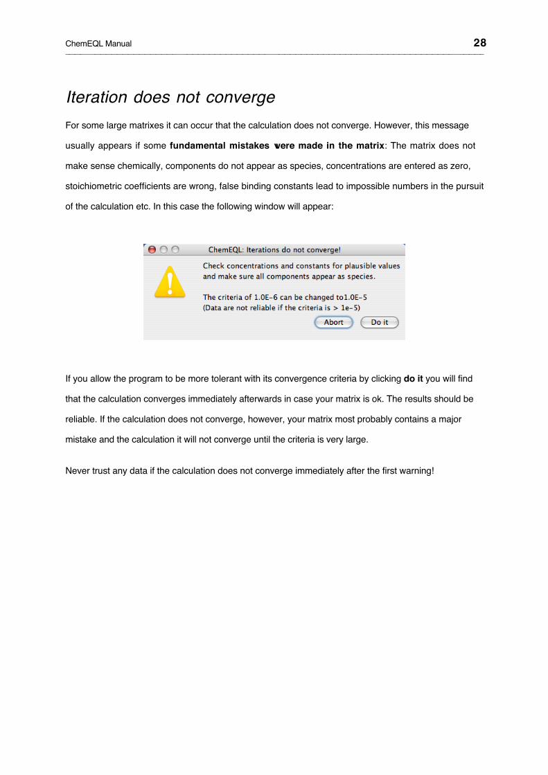
Iteration does not convergeFor some large matrixes it can occur that the calculation does not converge. However, this message

usually appears if some fundamental mistakes were made in the matrix: The matrix does not

make sense chemically, components do not appear as species, concentrations are entered as zero,

stoichiometric coefficients are wrong, false binding constants lead to impossible numbers in the pursuit

of the calculation etc. In this case the following window will appear:

If you allow the program to be more tolerant with its convergence criteria by clicking do it you will find

that the calculation converges immediately afterwards in case your matrix is ok. The results should be

reliable. If the calculation does not converge, however, your matrix most probably contains a major

mistake and the calculation it will not converge until the criteria is very large.

Never trust any data if the calculation does not converge immediately after the first warning!

ChemEQL Manual

29

How to set up a Matrix – The Details

The computer-compatible formulation of chemical reactions is designed in a matrix format. To describe

the species of interest (e.g. for acetic acid: HAc, Ac-), a minimum number of independent

components are chosen (e.g. HAc and H+, or Ac- and H+, or Ac- and OH-…) such that the formation

of all species can be written with chemical mass action laws as the products of the components and

binding constants. (no. of components = no. of species minus no. of independent reactions). The

stoichiometric coefficients of the components whose reactions form the species of interest appear in

the matrix; the components stand in the columns, the species in the lines of the matrix. The

equilibrium constants are added in an additional column. The matrices must be saved as EXCEL-text

files. The extension ‘.cql’ is recognized by the program as a ChemEQL file.

A simple example of a matrix is the following:

names of componentsmodes

names ofspecies

stoichiometriccoefficients

concentrations

formationconstants

Important!◆ The only condition with respect to the sequence of the components is to put H+ in the

last column and in the last line of the matrix.◆ Each component must also appear as a species in the matrix (with log K=0),

except solid phases or surface charges.◆ Write the charges of species and components as a number of '+' or '-' characters in the

names, e.g. Pb++, PO4--- (imperative only for activity corrections).

ChemEQL Manual

30

The mode codes for the matrix:The characterization (or mode) of the components which is given by the chemical question (eg. this

component is a solid phase, the concentration of this component remains constant, this is a particulate

surface...) is introduced in the second line of the matrix by the following codes:

Dissolved

'total' the given concentration is the total concentration of this component.

' free' the given concentration is the free concentration of this species thatcorresponds to this component and shall remain constant (eg. constant pH,equilibrium with atmospheric CO2, free Mez+ constant, etc.).

Solid phases

'solidPhase' this component is a solid phase with activity=1.

'checkPrecip' to check if this component precipitates for a given concentration under thechosen conditions, or define the amount of a solid phase that can be dissolved.

Adsorption

ConstantCap, Diffuse/GTL, SternL, and TripleL (Model of choice, see examples ).

'adsorbent1', 'adsorbent2', ... 'adsorbent5' indicate different types of particles.

Several types of surface sites for one particle type (up to three are possible) are named:

'adsorbent1.1', 'adsorbent1.2' ..., the numbers meaning (which particle.which site).

The charges have to be named

'charge1.1' ... 'charge5.1' (for ConstantCap and Diffuse/GTL),

'charge1.1' 'charge1.2' ... 'charge5.1' 'charge5.2' (for SternL), and

'charge1.1' 'charge1.2', 'charge1.3' ... 'charge5.1' 'charge5.2', 'charge5.3' (forTripleL). The numbers mean (which particle.which charge)

ChemEQL Manual

31

Creating a matrix by handAssume you want to calculate the pH and the distribution of the protonated and deprotonated species

of a 10-3 molar solution of acetic acid in pure water:

1 st List all chemical species that occur in the system:

HAc, Ac-, OH- and H+

2 n d Look for a minimum amount of components with which you are able to formulate the chemical

formation of all your species (you need the chemical equilibrium formation constants, e.g. from

Martell and Smith, Critical Stability Constants, 1974-82). In our example this can be HAc and

H+. (Alternatively, the formation of the above species can be described with HAc and OH-, with

Ac- and H+, or Ac- and OH-).

3 rd Write chemical equations for the formation of species using only components:

formation of HAc: HAc ⇔ HAc log K1 = 0

formation of Ac-: HAc ⇔ Ac- + H+ log K2 = -4.73

formation of OH-: H2O ⇔ O H- + H+ log K3 = -14

formation of H+: H+ ⇔ H+ log K4 = 0

4 t h Write mass action expression for the species according to the above equations:

HAc = K1 . HAc1

Ac- = K2 . HAc1 . [H+]- 1

OH- = K3 . [H+]1

H+ = K4 . [H+]1

ChemEQL Manual

32

5 t h The above equations define the system completely. To read these equations with a computer

program, we put the stoichiometric coefficients, which are the exponents of the above

equations, into a matrix of the following setup: species form the lines, components the columns.

Formation constants are added to the line of the corresponding species:

HAc H+ {log K}Hac 1 0 0Ac- 1 -1 -4.73O H- 0 -1 -14H+ 0 1 0

6 t h The concentrations of the components are added at the end of the columns. We start out with

10-3 moles of HAc in one liter of pure water (no strong acid added, therefore the start total

concentration of H+=0). Calculation for a variety of concentrations is possible by just adding the

next concentrations in the subsequent lines (see example A).

Since the program needs to know the meaning of the concentration of the components (e.g.

are these total concentrations, or is one of them the concentration of the free species, or is one

of the components a solid phase or an adsorbing surface etc.) we have to define the mode of

each component. In our case the concentration of HAc is the total amount that is in the system

and such is H+. (In case you want to give the pH however, you have to give the concentration of

the free species H+ (which is measured as pH).)

A collection of all predefined codes was given above. For our example they are 'total' for both

HAc and H+. They are added underneath the component names. Modes are fixed codes that

are recognized by the program. Names of species and components can be anything (or

nothing); it's just a text, except 'H+’ in the last column so the program knows it's the pH.

The program needs to know the charges of the species and components (only in case activity

coefficients and thus ionic strength is calculated). Write charges as '+' or '-' characters, e.g.

Pb++, PO4---, etc.

ChemEQL Manual

33

This is the final format for our matrix! Remarks or information about the stability constants can be added

to the right of the stability constants in {parenthesis}. Write on an EXCEL spreadsheet and save it in

text format. The extension ‘.cql’ is recognized by the program as a chemical matrix. (The following

matrix is in your set of examples in the ‘demo’ folder and is called 'aceticAcid.mat'

HAc H+ {log K}total total

Hac 1 0 0Ac- 1 -1 -4.73 {25 deg, I=0}O H- 0 -1 -14H+ 0 1 0

1 0-3 0

Start the program, read the matrix by choosing Open Matrix... from the File menu, and start the

calculation with Go in the Run menu. You will obtain the following output:

Data can be saved with Save Data... (recommended extension: .xls) and the matrix file with Save

Matrix… (recommended extension .cql) under the File menu.

ChemEQL Manual

34

Regular species distribution in homogeneoussolution

The simplest case for a speciation calculation is a system where all components are dissolved, and total

concentrations are known: A solution of 10-4 moles/l of PbCl2 in pure water.

Pb++, Cl- and H+ are selected for components. The combination of these three components

describes the formation of all species. (Of course one can choose other components as well, such as

PbOH+ and OH- if you wish for some reason). The components are selected from the library, with the

corresponding concentrations. The matrix looks as follows:

This matrix is in the demo folder and called 'PbCl2.mat'. The remarks to the right of the complex

formation constants give information on the conditions and origin of the constants: The first number

indicates the temperature and the second number the ionic strength at which the constants were

determined. Binding constants are from Smith&Martell: Smith and Martell, Critical Stability Constants

(1976).

ChemEQL Manual

35

Go from the Run menu produces the following datasheet. You find that pH of the solution is 5.85, and

that chloro complexes are negligible:

You might want to calculate a speciation for a constant pH. In that case you must change the 'mode' of

the 'H+' component from ‘total’ to 'free' since you want the free concentration of H+ to be a certain

value. Click in the mode code in the matrix window will produce a pop up menu that lets you change

the mode:

To change the concentration of H+ just enter ‘1e-8’ in the number field in the interactive matrix window.

Go will calculate the speciation of the system with 10-4 moles of PbCl2 in 1 liter of water at a pH of 8. Note

that you had to remove 7.74.10-5 moles of H+ from that system in order to sustain a pH of 8:

ChemEQL Manual

36

With Activity… binding constants are corrected for ionic strength either with Debye-Hückel,

Güntelberg, or Davies approximation. It is imperative that binding constants in the matrix are valid for I=0

and that charges of all components and species are present as ‘+’ and ‘-‘ characters. There is the option

to define a ionic strength or let the program calculate the ionic strength that results from the

concentration input data of your matrix (for more information see section 'Activity'). For our system with

10-4 mol/l PbCl2 the data sheet will give both concentrations and activities. Differences between

concentrations and activities in this system are very small:

ChemEQL Manual

37

In order to display the pattern of Pb species in a pH range choose pH range... from the Option

menu and enter the range of interest in reasonable steps, e.g. from 5 to 14 in steps of 0.25 pH units.

Represent the curves graphically for better overview by choosing Graphics... from the Options

menu and select the species of interest. This will produce the following output:

A datasheet that can be saved is printed in the back of the plot.

ChemEQL Manual

38

Octanol-water and gas-water distributionEquilibrium calculations that contain octanol-water distribution, gas-water (Henry)

coefficients or dissolution of organic substances can easily be included in speciation calculations.

Use the octanol-water or Henry coefficients in the same way as regular formation constants are used to

characterize the species.

ChemEQL Manual

39

Solid phases: dissolution and precipitation

Put up a matrix to calculate solubilityWe use the dissolution of Al(OH)3(Gibbsite) as an example to demonstrate the calculation when one (or

more) component(s) is a solid phase:

Al-species must be described using the solubility product of the solid phase, Al(OH) 3(Gibbsite). Collect

‘Al+++’ and ‘H+’ from the Regular Library (Access Library…):

Then insert ‘Al(OH)3(Gibbsite)’ to replace ‘Al+++’ (Insert Solid Phase…):

ChemEQL Manual

40

The equation for which the solubility product is valid is shown in the gray text field. Replacement can

be performed only if the matrix contains all components that occur in this equation (an error message

will occur if this is not the case). The active text field allows you to enter your own solubility constant if

you do not want to use the one given by the library. If the setting is correct the program will introduce

the solid phase in the matrix, recalculate all stoichiometric coefficients and binding constants, set the

mode to 'solidPhase' and the activity = 1:

(This matrix is stored in the ‘demo’ folder as 'Al(OH)3.cql')

DissolutionThe above matrix characterizes the dissolution of a chunk of Gibbsite in pure water (without CO2).

Calculation will result in the composition of the solution in thermodynamic equilibrium and the amount

of Gibbsite dissolved (2.58.10-8 mol/l):

ChemEQL Manual

41

Dissolution in acidic solution

Of course you can dissolve a lot more Gibbsite when the solution is acidified. Lets add, say 10-3 moles

of strong acid: change the concentration of ‘H+’ in the interactive matrix window, but leave the mode

‘total’. Then start the calculation. We end up with a solution of pH about 3.9 and 2.985.10-4 moles

Al(OH)3(Gibbsite) dissolved:

Dissolution at constant pH

Changing the mode from ‘total’ to ‘free’ indicates a system where pH is held constant at pH = 3. The

result sheet shows that 0.13 mol Gibbsite was dissolved in one liter, and that 0.39 mol H+ was needed

per liter to keep the pH constant at 3.0:

ChemEQL Manual

42

Graphical representation of solubility over a pH range

Calculate the solubility of Gibbsite in the natural pH range of water and display the result logarithmically

versus pH (log-log plot): Change the mode of ‘H+’ from ‘total’ to ’free’ with the pop up menu in the

matrix window. Then choose a pH range… (Options menu) from 3 to 8 in steps of 0.2. Select

Graphics… (Options menu) and mark the first 5 Al-species. Finally, change the Format (Options

menu) from ‘Linear’ to ‘Logarithmic’. Go in the Run menu will produce the following plot:

PrecipitationThe code ‘checkPrecip’ allows to test if a solution of given composition is oversaturated or

undersaturated with respect to a solid phase. For an example, we start with a solution of 10-6 moles of

Gibbsite in a solution of pH 2 and want to know when Gibbsite precipitates (if at all) if we rise the pH

continuously, e.g. during a titration.

ChemEQL Manual

43

This task can be accomplished with the same matrix. Change the mode code of 'Al(OH)3(Gibbsite)' from

'solidPhase' to 'checkPrecip'. The component now stands for total Al in the system and requires a

concentration. Enter ‘1e-6’. Adjust the concentration of ‘H+’ to ‘1e-2’ and make sure the mode is

‘free’, indicating constant pH. The matrix now looks like this:

To check for the pH region where precipitation possibly occurs choose a pH region, eg from 2 to 10 in

steps of 0.5 (pH range... in the Option menu), then Go. You will get the following datasheet:

ChemEQL Manual

44

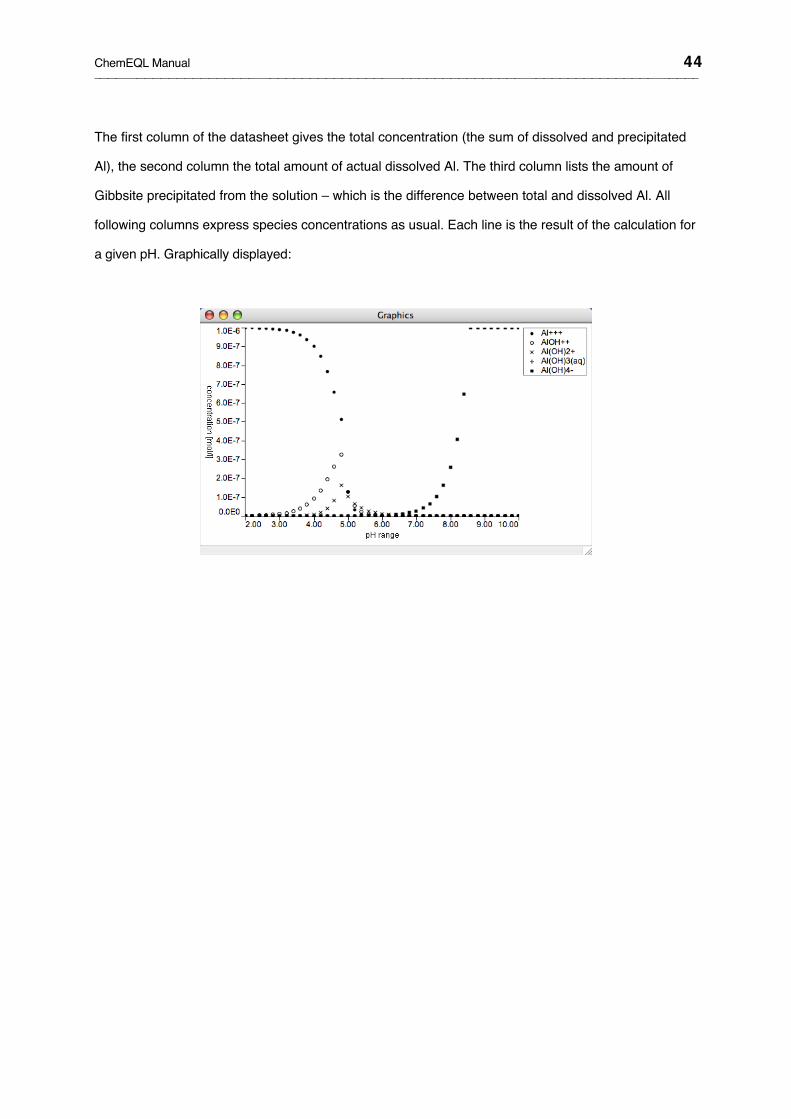
The first column of the datasheet gives the total concentration (the sum of dissolved and precipitated

Al), the second column the total amount of actual dissolved Al. The third column lists the amount of

Gibbsite precipitated from the solution – which is the difference between total and dissolved Al. All

following columns express species concentrations as usual. Each line is the result of the calculation for

a given pH. Graphically displayed:

ChemEQL Manual

45

Adsorption to particulate surfaces

Introduction to the principles of surface adsorptionThis chapter gives a short introduction of the ideas of adsorption models, the information needed to

implement the various electrostatic models in ChemEQL, and how to include the specific surface

parameters in the matrix. For detailed discussion of the models as well as good reviews see Dzombak

and Morel (1990), J. Westall and H. Hohl (1980), or Stumm and Morgan (1996).

The free energy of adsorption actually consists of a chemical term describing the chemical

interactions, and an electrostatic term accounting for electrostatic attraction and repulsion that

occur at interfaces:

ΔG = ΔGchemical + ΔGelectrostatic

The electrostatic term can be looked at as a type of activity coefficient that has to be taken into account

for adsorption reactions of charged species. The coulombic term expresses the work needed to

transport n charges through a potential gradient Ψ:

ΔGelectrostatic = nFΨ

where F the Faraday constant (electrical charge of 1 mole of electrons) and Ψ the surface potential in

Volts. Since ΔGchemical = -RT ln K we can write adsorption reaction constants as

K = Kint . exp(-nFΨ/RT)

R is the molar gas constant and T the absolute temperature. The exponential term is compatible with

the chemical potential term and can therefore be included in the set of components. The formation of

adsorbed species can now be described by introducing their charge in the column with the

exponential term in addition to the chemical interaction. The concentration that is to put for this column

is the total sum of all surface charges:

Ptot = ({≡SOH2+} + {≡SOPb+} + ...) - ({≡SO-} + ...)

ChemEQL Manual

46

or expressed as a charge: σ = Ptot . F/SA

where S is the specific surface area, and A the concentration of solid.

Different relationships between charge and surface potential can be thought of and therefore various

models were created accordingly, the most simple one being the constant capacitance model where

charge and potential are related only through the capacitance C (see literature cited above):

σ = C . Ψ

The recent literature recommends to use the model of the Diffuse Double Layer (Dzombak and Morel,

1990; Stumm, 1997) where

€

s = (8RTεε0c ⋅103)12 sinh ZΨF

2RT

ε and ε0 are the dielectric constant of water and the permittivity of free space, respectively. c is the

molar electrolyte concentration, and Z the ionic charge.

How to put up an adsorption matrix: A simple example:Pb adsorbs to Fe-oxide particles under near neutral and alkaline conditions. We need additional

information on the nature and chemical behavior of the suspended particles such as: Specific surface

area, concentration of surface sites, ionic strength and capacitance of the electric double layer. Choose

the model you wish to use to account for the electrostatic interactions between charges: You have the

choice of either the Constant Capacitance Model ('ConstantCap'), the Diffuse Double Layer Model or

the Generalized Two Layer Model ('Diffuse/GTL'), the Basic Stern Layer Model ('SternL') or the

Triple Layer Model ('TripleL'). With ChemEQL you have the possibility of choosing either (up

to five) different types of adsorbents or (up to three) different types of surface sites

on one type of adsorbent.

ChemEQL Manual

47

Adsorbing surface sites and surface charges are introduced in the matrix as components. We assume

here one type of particle with one type of surface site, and the formation of two types of surface

complexes which differ only in stoichiometry, modeled as mono- and bidentate surface complexes of

Pb. Adsorption matrices cannot be put up from the library but must be organized in EXCEL. In the

adsorption matrix surface site(s) are treated like ordinary ligands:

FeOOH -> [FeOOH] = 100. [FeOOH]

FeOOH ⇔ FeOO- + H+ [FeOO-][H+][FeOOH] = 10-9 -> [FeOO-] = 10-9.[FeOOH][H+]-1

FeOOH + H+ ⇔ FeOOH2+

[FeOOH2+][FeOOH][H+]

= 106.7 -> [FeOOH2+] = 106.7.[FeOOH][H+]

Pb2+ -> [Pb+2] = 100. [Pb+2]

FeOOH + Pb+2 ⇔ FeOOPb+ + H+ [FeOOPb+][H+][FeOOH][Pb+2]

= 10-0.52 -> [FeOOPb+] = 10-0.52.[FeOOH][Pb+2][H+]-1

2FeOOH + Pb+2 ⇔ (FeOO)2Pb + 2H+[(FeOO)2Pb][H+]2

[FeOOH]2[Pb+2] = 10-6.27 -> [(FeOO)2Pb] = 10-6.27.[FeOOH]2[Pb+2][H+]-2

Add the additional information required at the bottom of the matrix as shown in the following example.

Make sure to use correct codes for double layer models and correct modes for components: The

column containing the particulate ligand must be called 'adsorbent1' (you can have up to five

different particles; see further examples. Call them 'adsorbent2', 'adsorbent3' etc.). If you wish to

use different types of surface sites (up to three are possible) call these components 'adsorbent1.1',

'adsorbent1.2' etc. The numbers indicate 'adsorbent(whichParticle.whichSite)'. Columns containing

charges must be called 'charge1.1', 'charge2.1', etc for Constant Capacitance and Diffuse Double

Layer models. The Triple Layer model requires three charge components: 'charge1.1',

'charge1.2', 'charge1.3' for each adsorbing type of particles, the numbers indicating

'charge(whichParticle.whichCharge)'. See examples 11-16 later.

ChemEQL Manual

48

0 is entered for the concentration of adsorbent (since the program will calculate concentrations from

the input of other parameters and does not require this input), and 0 for the sum of charges (for

Constant Capacitance and Diffuse Layer models where there is only one double layer).

The above matrix is located in the demo folder and is named 'FeAdsorption.cql', and calculation

can be performed directly. The lower part of the data window contains the total concentration of

adsorption sites as calculated from the input of specific surface area, number of active surface sites,

and concentration of adsorbent. The total concentration of surface charges sums up all charges of

surface species and expresses them in moles per liter.

Titration of a solution with particlesIf you use matrices with adsorption to particulate surfaces you have the additional option to titrate your

system with particles, ie. to vary the particle concentration in a specified range, much similar

ChemEQL Manual

49

to the option of varying the concentration of a component. Choose Adsorption range... from the

Options menu, and enter the range of concentrations of your particulate matter.

The Generalized Two Layer ModelDzombak and Morel in their first compilation of experimental adsorption data recommend for pragmatic

reasons the use of the Generalized Two Layer Model. The Generalized Two Layer Model

basically consists of the Diffuse Double Layer Model combined with the Surface

Precipitation Model by Farley et al (1985), which can account for the eventual formation of a solid

solution phase on the surface at high sorbate to sorbent ratios. The diffuse layer model considers one

layer of surface charges and a diffuse layer of counter charges in solution. A capacitance is not

needed. The authors recommend using one surface site to model anion adsorption data, and two site

types ('strong' and 'weak' surface sites, both site types are considered to have the same

proton binding characteristics!) to model cation adsorption data. They find this basic two-layer

model adequate for the description of all but the highest cation concentrations. An example for the

cation surface complexation with two site types on one sort of particles as recommended by Dzombak

and Morel, however without surface precipitation, is given below. (Example 4.2). It is named 'GTL.mat'

in your demo folder.

ChemEQL Manual

50

Note that no capacitance is needed in the input matrix. At high sorbate/sorbent ratios precipitation of

the hydroxide or carbonate of the adsorbing cation on the surface was observed by Farley et al.

(1985). Their model considers the formation of a new surface phase. To describe the formation of a

'solid solution' on the surface solubility products determined for bulk solutions are applied. All surface

reactions need to be described as surface precipitation reactions. A new component is introduced in

order to describe the fractions of sorbate and sorbent in the solid solution. An example for the sorption

and precipitation reactions of a cation M2+ on a hydrous oxide X(OH)3(s) is taken from Dzombak and

Morel (1990), p. 29-32:

Adsorption of M2+ on X(OH)3(s):

€

≡ XOH 0 + M 2+ + 2H2O↔ X(OH)3(s)+ ≡ MOH2+ + H + KM

app

Precipitation of M2+:

€

≡ MOH2+ + M 2+ + 2H2O↔M(OH)2(s)+ ≡ MOH2

+ + 2H + KspM-1

Precipitation of X3+:

€

≡ XOH 0 + X 3+ + 3H2O↔ X(OH)3(s)+ ≡ XOH0 + 3H + KspX

-1

ChemEQL Manual

51

The adsorption reaction of X3+ on M(OH)2(s) can be derived from the above equations and is not

shown. The component Ts represents the total mass of solid material in solid solution and is used to

express the activity constraint on the solid solution.

The matrix that results from this input and suits the need of the complete 'Generalized Two Layer

Model' for cation adsorption including surface precipitation looks like represented in the following table

('GTL-Precip.table' in the demo folder) and only needs to be completed with the appropriate formation

constants and concentrations:

Surfaces characterized by Fractional Surface Charge:The one-pK-modelThe one-pK-model (Westall, 1987) simplifies the description of the acid-base equilibria by assuming

only one proton exchange reaction. (The following example and more are published and discussed in

the 2nd ed. of Stumm, 1992):

ChemEQL Manual

52

€

SOH2+ 12 ↔ SOH− 12 + H + Ka

In fact, a new uncharged component, SOH01.5, was introduced to allow the equilibria to be described

with only one protolysis constant:

€

SOH2+ 12

−12H +

← → SOH1.50 −

12H +

← → SOH− 12

€

Ka12

€

Ka12

The matrix therefore needs the uncharged surface species as a component, and the two species with

broken charges:

The program calculates the total concentration of surface sites from the entries of the concentration of

adsorbent [kg l-1] and the characteristic conc. of surface sites [mol kg-1]. In the column of the surface

charges of the species are the differences in surface charge for the reaction considered. The potential

difference across the double layer is calculated according to the model chosen, preferably the Diffuse

Double Layer model.

Anion or cation sorption is introduced with the following type of equations:

cation:

€

SOH− 12 + Me2+ ↔ SOMe+ 12 + H +

anion:

€

SOH− 12 + HA↔ SA− 12 + H2O

ChemEQL Manual

53

ExamplesThe next three examples show basic input matrices for the four different models. Further examples in

the 'examples' chapter will demonstrate the use of several types of adsorbents.

Example for a basic matrix of surface speciation according to the Constant Capacitance Model

('ConstantCap.mat' in demo folder):

Example for a basic matrix of surface speciation according to the Diffuse Layer Model, which is

recommended to use by Dzombak and Morel ('Diffuse/GTL.mat'):

Surface speciation according to the Basic Stern Layer Model:

ChemEQL Manual

54

Surface speciation according to the Triple Layer Model:

Literature:Dzombak D.A., and F.M.M. Morel: Surface Complexation Modelling. Wiley Interscience (1990).

Farley K.J., D.A. Dzombak, F.M.M. Morel: A surface prepcipitation model for the sorption ofcations on metal oxides. J. Colloid Interface Sci. 106, 226-242 (1985).

Stumm W., and J.J. Morgan: Aquatic Chemistry, 3rd ed. (1996).

Stumm W.: Chemistry of the solid-water interface. Wiley Interscience, 1992.

ChemEQL Manual

55

Westall J., and H. Hohl: A comparison of electrostatic models for the oxide-solutioninterface. Adv. Coll. Interface Sci., 12, 265-294 (1980).

Westall J.: Adsorption mechanisms in aquatic surface chemistry. in: Aquatic surfacechemistry, ed. by W. Stumm, John Wiley and Sons, New York, 3-32 (1987).

ChemEQL Manual

56

Redox Reactions

The (microbially mediated) redox equilibrium between N(V) and N(-III) is calculated as an example. The

electron, which is part of these reactions, must be a component. The following equations are in the

library and can be accessed easily:

NO3- -> [NO3

-] = 100. [NO3-]

NO3- + 9H+ + 8e- ⇔ NH3 + 3H2O

[NH3][NO3-][H+]9[e-]8

= 10109.9 -> [NH3] = 10109.9.[NO3-][e-]8[H+]9

NO3- + 10H+ + 8e- ⇔ NH4

+ + 3H2O[NH4+]

[NO3-][H+]10[e-]8 = 10119.2 -> [NH4

+] = 10119.2.[NO3-][e-]8[H+]10

2H2O ⇔ O2(g) + 4H+ + 4e- [O2(g)][e-]4[H+]4) = 10-83 -> [O2(g)] = 10-83[e-]-4[H+]-4

2H+ + 2e- ⇔ H2(g)

[H2(g)][e-]2[H+]2

= 100 -> [H2(g)] = 100.[e-]2[H+]2

e- -> [e-] = 100. [e-]

H+ -> [H+] = 100. [H+]

ChemEQL Manual

57

This matrix is stored in the demo folder under the name 'Redox.mat'

To represent the development of the N(V)-N(-III) couple in a pε-range choose Component range...

from the Options menu. Select the e- component and enter a logarithmic interval from -8 to -2 in

steps of 0.25. (The output format is now set to logarithmic as you can check in the Format item).

Select Graphics... and mark the first five items to obtain the curves. Go will calculate the following

graph:

NO3- prevails in the region where log e- is smaller than -5.5, and NH4

+ under more reducing conditions

where log e- >-5.5.

ChemEQL Manual

58

Kinetics

ChemEQL allows the calculation of species distribution in a system that is controlled by one rate

limiting chemical reaction. The chemical speciation is assumed to be much faster than the selected

kinetic reaction. The program covers the most common types of kinetic rate equations. (No

consecutive kinetic reactions are possible, however.)

In a first step the program performs a speciation calculation that results in the concentrations of the

species before any kinetic reaction takes effect (tkin = 0). The equilibrium concentration of the educt

species (E) is then set to the start concentration of the educt for the kinetic calculation. The following

kinetic calculation therefore uses the concentration of the educt species (and not the total

concentration of the educt component). The amount of E used up in this process is subtracted from

the total concentration of E, and the product (P) produced by this step is added to the total

concentration of P. A speciation calculation is then performed and the result given in the output. If the

kinetic reaction is reversible (includes a backreaction) or autocatalytic (product enhances speed of

reaction), the concentration of P that takes part in the kinetic calculation is of course also the free

concentration of the product species and not the total concentration of P.

The input matrix must be organized such that educt and product are components:

Educt Product . . . H + {log K}total total . . . . . .

Educt 1 0 0 0 0Product 0 1 0 0 0ProdSpecies1 ... ... ... ... ...ProdSpecies2 ... ... ... ... .... . . ... ... ... ... ...OH- 0 0 0 -1 -14H + 0 0 0 1 0

startConc usually=0 . . . . . .

ChemEQL Manual

59

Be aware of the dimensions of the kinetic constants! Use moles l-1 sec-1 (zero order), sec-1 (1st

order), l moles-1 sec-1 (2n d order) etc. or remember that the time scale of your input will change

the output accordingly.

The following dialog appears if you choose Kinetics... from the menu:

Choose the desired rate law, define educt and product of your system, enter the stoichiometric

coefficients, rate constants, and time interval. For graphical display of one or more species choose

Graphics... from the Options menu after closing the kinetic dialog.

A few basic examples for simple Kinetic calculations without speciation are given below. The following

general matrix can be used to demonstrate the function of all types of kinetics:

ChemEQL Manual

60

Zero order:

(k=10-3, t=5-100)

First order:

(k=0.01, t=10-300)

Reversible:

(k=0.05, kback=0.05, t=2-50)

ChemEQL Manual

61

Second order in C:

(k=1, t=2-50, logarithmic scale)

Second order overall, but first order in C

and D: (k=1, t=2-50, logarithmic scale)

Autocatalysis: (k=14.6, t=0.5-10,

Example see Frost&Pearson, Kinetics and

Mechanism, Wiley 1961, p19)

Third order:

(k=100, t=1-20, logarithmic scale)

ChemEQL Manual

62

Integrated rate laws

zero order: cC → P

€

C[ ]t = C0 − ckt

first order: cC → P

€

C[ ]t = C0 ⋅ exp−ckt

C ↔ P (reversible)

€

C[ ]t = C0k + ′ k ⋅ exp k + ′ k ( )t

k + ′ k ( ) ⋅ exp k + ′ k ( ) t

Second order: cC → P

€

C[ ]t =C0

C0ckt +1

cC + dD → P

€

C[ ]t = C0 −cC0D0 exp

kt C0−D0( )−1( )dC0 exp

kt C0−D0( )− cD0

€

D[ ]t = D0 −dcC0 −Ct( )

cC → pP (autocatalysis)

€

C[ ]t =1cC0 −

C0P0 p ⋅ expkt C0 +P0( )− c( )

cC0 + pP0 ⋅ expkt C0 +P0( )

€

P[ ]t =1cC0 + P0 − c C[ ]t{ }

Third order: cC → P

€

C[ ]t =C0

2cktC02 +1

nth order: cC → P

€

C[ ]t =C0

n −1( )cktC0n−1 +1( )1n

ChemEQL Manual

63

pX-pY diagrams

The pX-pY diagrams option is of use in the calculation of the prevailing dissolved species or solid

phases of a component under varying conditions of another parameter like the redox potential

(pε), a complex forming ligand, or a ligand that forms solid phases with the component.

Calculation is possible only for species derived from one single component (eg. all dissolved

complexes and solid phases for Fe(II) and Fe(III) if either Fe2+ or Fe3+ is chosen as a component).

All relevant species that are to appear in the diagram must have priority in the

list of species. Species that are solid phases must carry the code '(s)' in their

names, gaseous species the code '(g)', so the program can recognize them.

The option shall be demonstrated with two examples: 1) The calculation of the pε-pH-diagram

for water, and 2) the pε-pH-diagram for the Fe-CO2-system as exemplified in Stumm and Morgan,

Aquatic Chemistry (1981), p. 446.

Example 1: pε-pH-diagram for waterWhat are the redox boundaries for the existence of water? At what pH and redox potential is H2O

either reduced or oxidized?

The species occurring in the system are: H2O, H2(g), O2(g), e-, OH-, and H+

Three reactions have to be taken into consideration:

a. the oxidation: 2H2O ⇔ O2 + 4e- + 4H+ log K = -83

b. the reduction: 2H+ + 2e- ⇔ H2 log K = 0

c. autocatalysis of water: H2O ⇔ H+ + OH- log K = -14

ChemEQL Manual

64

The program calculates speciation in the desired steps, searches for the species with the

highest concentration, and compares with the species with the highest concentration found in

the last interval. Gaseous species (whose name must contain the code '(g)') are recognized as

dominating when their partial pressure is at least 1atm, and solid phases '(s)' when their

solubility product is exceeded. Bordering concentrations are calculated by an iterative

procedure converging when the error is smaller than .001.

The abovementioned six species are described with three components (H2O, e-, and H+), and

constitute the input matrix. Input concentrations are 55.55 mol/l for water, and any concentration

for e- and H+, since these concentrations will be altered by the program according to user inputs

by the pX-pY-dialog. The modes for these two components must be 'free'. (The matrix is 'pXpY-

H2O.mat' in the demo folder):

H2O e - H+total f ree f ree

O2(g) 2 -4 -4 -83H2(g) 0 2 2 0H2O 1 0 0 0e - 0 1 0 0O H - 0 0 -1 -14H+ 0 0 1 0

5 5 . 5 5 1e+3 1 e - 3

Choosing pXpY diagram... from the menu will lead you to the following dialog window:

ChemEQL Manual

65

Choose the X and Y component and give the range in negative logarithms (pX = -log X). Choose

pH range 3 to 9 and pε range -10 to +20. The main component that is common to all

species of interest is H2O. Species from 1-3 are to be included in the graphic (i.e. O2 (g), H2

(g), H2O). The suggested step size of 0.2 refers to the logarithmic units of both, pX and pY, i.e.

pH and pε.

Filling in the questionnaire, closing, and pressing Go will automatically activate Graphics,

and you will obtain the following diagram:

ChemEQL Manual

66

Save the calculated points that appeared in the data window by choosing Save data... from

the File menu to use a professional drawing software.

Example 2: pε-pH-diagram for the Fe - CO2 - H2Osystem(from Stumm and Morgan, Aquatic Chemistry, 1981, fig. 7.7.)

The various dissolved complexes and solid phases of iron, reduced and oxidized, that prevail

under certain conditions of pH and redox potential are calculated here according to thermo-

dynamic equilibrium constants. It is quite a task to collect all equilibrium constants, and

comparing them with the constants used in Stumm and Morgan or Sigg und Stumm (Aquatische

Chemie, 1994), one will find that these are not consistent throughout the graphs. Small

changes in the solubility products for Fe(OH)2(s) and FeCO3(s) lead to marked differences in the

region of existence for FeCO3 (s).

Reactions relevant to the system and its constants are collected in the following matrix ('pXpY-

Fe.mat' in the demo folder). Note that the formation of all iron species is formulated with Fe2+:

Fe++ HCO3- e - H+total total f ree f ree

Fe++ 1 0 0 0 0FeOH+ 1 0 0 -1 -9.5Fe(OH)2(aq) 1 0 0 -2 -20.6Fe(OH)3- 1 0 0 -3 -31Fe(OH)2(s) 1 0 0 -2 -12.1FeCO3(aq) 1 1 0 -1 -5.6FeHCO3- 1 1 0 0 2.4FeCO3(s) 1 1 0 -1 0.2Fe(s) 1 0 2 0 -13.8Fe+++ 1 0 -1 0 -13.0FeOH++ 1 0 -1 -1 -15.2Fe(OH)2+ 1 0 -1 -2 -20.2Fe(OH)4- 1 0 -1 -4 -35.2Fe(OH)3(s) 1 0 -1 -3 -16.0H2CO3 0 1 0 1 6.3HCO3- 0 1 0 0 0CO3-- 0 1 0 -1 -10.3e- 0 0 1 0 0OH- 0 0 0 -1 -14H+ 0 0 0 1 0

1 . 0 E - 5 1 . 0 E - 3 1 .0E+71 . 0 E - 7

ChemEQL Manual

67

The diagram is calculated for a total iron concentration of 10-5 mol/l and a total bicarbonate

concentration of 10-3 mol/l. Combined with the data from example 1, the diagram looks as follows

and can easily be completed with a few lines:

- 1 5

- 1 0

- 5

0

5

10

15

20

0

-log

e-

5 10 15

pO2 > 1atm

pH2 > 1atm

pH

Fe+2

Fe(s)

FeCO3(s)

Fe(OH)2(s)

Fe(OH)3(s)

Fe(OH)4-

Fe+3

FeOH+2

The square in the lower right corner was calculated with higher resolution to clearly recognize

the slope of the border between Fe(OH)2(s) and Fe(OH)4-.

ChemEQL Manual

68

Examples

1 . All components dissolved, total concentrations givenComplexes of Pb(II) with EDTA and NTA ex01.matTitration curve for Na3PO4 with acid ex02.matTitration curve for H3PO4 with base ex03.mat

2 . All components dissolved, free concentrations of some components are givenconstant pH: Complexes of Mercury (II) ex04.matconstant pCO2: Equilibrium with a soda solution ex05.matconstant free conc. of a species: Metal buffer for Cu2+(aq) ex06.mat

3 . Dissolution of one (or more) solid phaseDissolution diagram of Cu(OH)2(s) ex07.matThe CaCO3 / CO2 - system ex08.matDissolution of Ca4Al2O6SO4

.12H2O ex09.matDissolution of several solid phases ex10.mat

4 . Precipitation of one (or more) solid phasesPrecipitation of PbCO3(s) ex11.mat

5 . Adsorption to particulate surfaces-one particulate surface or one type of surface site respectivelySurface speciation of γ-Al2O3 in 0.1M NaClO4 at pH 7

Constant Capacitance Model ex12.matDiffuse Layer Model / Generalized Two Layer Model ex13.matBasic Stern Layer Model ex14.matTriple Layer Model ex15.mat

Adsorption of lead on goethite ex16.mat

-two or more particulate surface typesConstant Capacitance Model ex17.matDiffuse Layer / Generalized Two Layer Model ex18.matBasic Stern Layer Model ex19.matTriple Layer Model ex20.mat

-Several types of surface sites on one type of particle

ChemEQL Manual

69

Diffuse Layer / Generalized Two Layer Model ex21.mat6 . pXpY Diagrams

The S(VI), S(0), S(-II) - System ex22.matThe Chlorine System ex23.mat

7 . Solubility DiagramsThe Iron - CO2 System ex24.matThe PbCO3 - PbSO4 System ex25.mat

ChemEQL Manual

70

1. All components dissolved, totalconcentrations given

Complexes of Pb(II) with EDTA and NTA(ex01.mat)Equilibrium concentrations of all species in a solution made from 10-6 M Pb(II), 2.10-6 M H4EDTA

and 10-5 M Na3NTA:

Pb++ H4EDTANTA--- H+total total total total

Pb++ 1 0 0 0 0PbOH+ 1 0 0 -1 -7.7Pb(OH)2 1 0 0 -2 -17.1Pb(OH)3- 1 0 0 -3 -28.1PbNTA- 1 0 1 0 12.6PbEDTA-- 1 1 0 -4 -3.96PbHEDTA- 1 1 0 -3 -0.76EDTA---- 0 1 0 -4 -23.76HEDTA--- 0 1 0 -3 -12.64H2EDTA-- 0 1 0 -2 -3.66H3EDTA- 0 1 0 -1 -2.72H4EDTA 0 1 0 0 0NTA--- 0 0 1 0 0HNTA-- 0 0 1 1 9.71H2NTA- 0 0 1 2 12.19H3NTA 0 0 1 3 13.99H4NTA+ 0 0 1 4 14.79OH- 0 0 0 -1 -14H+ 0 0 0 1 0

1 e - 6 2 e - 6 1 e - 5 0

Choose Go from the Run menu...

ChemEQL Manual

71

Titration of Na3PO4 with strong acid (ex02.mat)Say we want to calculate the Titration of a 10-3 M solution of Na3P O4 with strong acid:

The matrix can be collected from the library. Na+ is omitted since it does not take part in any

reaction.

PO4- - - H+total total

PO4--- 1 0 0HPO4-- 1 1 12H2PO4- 1 2 18.8H3PO4 1 3 20.9OH- 0 -1 -14H+ 0 1 0

1 e - 3 0

Choose Component range from the Option menu. Select H+ (since we titrate with strong

acid) and give a range for the amount of strong acid added per liter, eg. from 0 to 3e-3 in steps of

1e-4. (A remark will follow your attempt to enter a concentration of 0, and it will be changed to a

very small number). If you wish a graphical representation of the titration curve, change the

output format from linear to logarithmic (since we want to see the pH in dependence of acid

added), select the 'H+' species in the Graphic item of the Options menu, and press Go:

ChemEQL Manual

72

Titration of H3PO4 with strong base (ex03.mat)Calculate a titration curve to the titration of a 10-3 M solution of H3PO3 with strong base! For this

task select a matrix with ‘H3PO4’ and ‘H+’, then choose Replace H+ by OH- from the Matrix

menu. You should obtain:

H3PO4 O H -total total

PO4--- 1 3 21.1HPO4-- 1 2 19.1H2PO4- 1 1 11.9H3PO4 1 0 0H+ 0 -1 -14OH- 0 1 0

1 e - 3 0

Choose Component range under the Option menu and give a range for the amount of OH-

added per liter (eg. from 0 to 3.10-3 in steps of 10-4). For graphical representation of the titration

curve (pH vs. base added) choose the 'H+' species in Graphics… and change the format from

linear to logarithmic. The following titration curve should be obtained:

ChemEQL Manual

73

2. All components dissolved, freeconcentrations of some components given

Constant pH: Complexes of Hg(II) with hydroxideand chloride (ex04.mat)What is the distribution of mercury species in a solution with 10-9 M Hg(II), 0.1M Cl- and pH 8.3 ?

Choose Hg++, Cl-, and H+ as components and put up the matrix:

Hg++ Cl- H+total total f ree

Hg++ 1 0 0 0HgOH+ 1 0 -1 -3.4Hg(OH)2 1 0 -2 -6.2Hg(OH)3- 1 0 -3 -21.1Hg2OH+++ 2 0 -1 -3.3HgCl+ 1 1 0 6.72HgCl2 1 2 0 13.23HgCl3- 1 3 0 14.2HgCl4-2 1 4 0 15.3Cl- 0 1 0 0OH- 0 0 -1 -14H+ 0 0 1 0

1 e - 9 0 . 1 5 e - 9

ChemEQL Manual

74

Constant pCO2: Equilibrium of a soda solution withatmospheric CO2 (ex05.mat)10-4 moles of soda (Na2CO3) are dissolved in one liter of water. A certain pH establishes

immediately. If this solution is left open to the atmosphere it will take up CO2 from the air, and the

pH will decrease until a new equilibrium is reached. What is this pH, and how much atmospheric

CO2 is taken up by this solution?

Solution: The solution gives up CO2 until equilibrium with the atmosphere is reached. If one

CO32- turns into CO2, two equivalent OH- remain in the solution according to the reaction:

CO32- + H2O ↔ CO2 + 2OH-

The final solution therefore corresponds to a solution of 2.10-4 M base that equilibrates with the

atmosphere. This is represented by the following matrix:

CO2(g) O H -f ree total

H2CO3 1 0 -1.4HCO3- 1 1 6.3CO3- - 1 2 10H+ 0 -1 -14O H - 0 1 0

3 . 5 e - 4 2 e - 4

ChemEQL Manual

75

Constant free concentration of a species: Metalbuffer for Cu2+

(aq) (ex06.mat)What is the total conc of Cu(II) in a metal buffer with a free Cu2+ concentration of 10-12 M, a Tris

concentration (Tris(hydroxymethyl)aminomethane) of 10-4 M at pH 7.5?

Cu++ Tris H+f ree total f ree

Cu++ 1 0 0 0CuOH+ 1 0 -1 -8Cu(OH)2 1 0 -2 -15.2Cu(OH)3- 1 0 -3 -26.8Cu(OH)4-- 1 0 -4 -39.9Cu2(OH)2++ 2 0 -2 -11CuTris++ 1 1 0 3.95Cu(Tris)2++ 1 2 0 7.63Cu(Tris)3++ 1 3 0 11.1Cu(Tris)4++ 1 4 0 14.1CuOHTris+ 1 1 -1 -2.05(CuOHTris)2++ 2 2 -2 1.9CuOH(Tris)2+ 1 2 -1 1.31Cu(OH)2(Tris)2 1 2 -2 -6.59Tris 0 1 0 0HTris+ 0 1 1 8.09OH- 0 0 -1 -14H+ 0 0 1 0

1e -12 1 e - 4 3 e - 8

The total concentration of copper can be read from the bottom part of the data window as the

sum of the 'free conc.' and the amount that had to be added in order to provide the desired

equilibrium situation, 'in or out of system'. -> Cutot = 9.60.10-12 M

ChemEQL Manual

76

3. Dissolution of one (or more) solid phase(s)

Dissolution diagram of Cu(OH)2(s) (ex07.mat)Calculate the maximum soluble copper in the pH range between 5 and 10 (log conc. vs. pH) if

Cu(OH)2 is the limiting phase! Use complexes of Cu(II) with hydroxide, carbonate and nitrate in

pure water in equilibrium with atmospheric pCO2 of 5.10-4 atm which contains 0.01 M NO3-:

Compile a matrix consisting of NO3-, Cu++, CO2 and H+, then replace Cu++ with Cu(OH)2(s)

using Insert Solid Phase…

NO3- Cu(OH)2 CO2 H+total solidPhase f ree f ree

Cu++ 0 1 0 2 8.68CuOH+ 0 1 0 1 0.68Cu(OH)2 0 1 0 0 -6.52Cu(OH)3- 0 1 0 -1 -18.12Cu(OH)4-- 0 1 0 -2 -31.22Cu2(OH)2++ 0 2 0 2 6.36CuCO3 0 1 1 0 -2.72Cu(CO3)2-- 0 1 1 -2 -16.83CuNO3+ 1 1 0 2 9.18Cu(NO3)2 2 1 0 2 8.28NO3- 1 0 0 0 0H2CO3 0 0 1 0 -1.5HCO3- 0 0 1 -1 -7.82CO3-- 0 0 1 -2 -18.15OH- 0 0 0 -1 -14H+ 0 0 0 1 0

1 e - 2 1 5 e - 4 1 e - 7

To calculate speciation for a pH range, choose pH range in the Options menu, enter the desired

range and step size (e.g. pH 5 to 10 in steps of 0.2 pH units). A logarithmic representation of the

Cu species looks as follows:

ChemEQL Manual

77

ChemEQL Manual

78

The CaCO3 – CO2 system (ex08.mat)What is the pH and composition of a water which is in equilibrium with calcite, CaCO3 and

atmospheric pCO2 (10-3.5 atm) ? How much CO2 and CaCO3 dissolve in one liter of pure water?

CaCO3 CO2 H+solidPhase f ree total

Ca++ 1 -1 2 9.7CaOH+ 1 -1 1 -2.5CaCO3(aq) 1 0 0 -5.3CaHCO3+ 1 0 1 3.3H2CO3 0 1 0 -1.5HCO3- 0 1 -1 -7.8CO3-- 0 1 -2 -18OH- 0 0 -1 -14H+ 0 0 1 0

1 . 0 3 .16e -4 0

pH is 8.265, 4.834.10-4 mol Calcite and 4.757.10-4 mol CO2 dissolve in the solution until

equilibrium is reached.

ChemEQL Manual

79

Dissolution of Ca4Al2O6SO4 .12H2O (ex09.mat)If Ca4Al2O6SO4

.12H2O dissolves congruently, stoichiometric amounts of Ca(II) and Al(III) are

released. What are the concentrations of totally dissolved Ca(II) and Al(III), and what is the pH of

the solution?

Ca4Al2O6SO4Al+++ SO4- - H+solidPhase total total total

Ca++ 0.25 -0.5 -0.25 3 18.6CaOH+ 0.25 -0.5 -0.25 2 5.75Al+++ 0 1 0 0 0AlOH++ 0 1 0 -1 -5Al(OH)2+ 0 1 0 -2 -9.3Al(OH)3 0 1 0 -3 -15Al(OH)4- 0 1 0 -4 -23SO4-- 0 0 1 0 0OH- 0 0 0 -1 -14H+ 0 0 0 1 0

1 0 0 0

Note that start concentrations are zero for all components except the solid phase. From the data

window you will find the total concentrations by addition of the respective species

concentrations:

Catot = 4.14.10-3 M, Altot = 2.07.10-3 M, and the pH = 11.59.

ChemEQL Manual

80

Dissolution of several solid phases (ex10.mat)What is the pH and composition of a 10-2 M solution for NO3

- which is in equilibrium with the

carbonate phases of Zn(II), Cd(II), Pb(II), and Cu(II), and atmospheric pCO2 (10-3.5 atm) ? Which

solid is the most soluble, which the least soluble?

ZnCO3(s) CdCO3(s)PbCO3(s) CuCO3(s) NO3 CO2(g) H+ {log K}solidPhase solidPhase solidPhase solidPhase total free total

Zn++ 1 0 0 0 0 -1 2 7.98ZnOH+ 1 0 0 0 0 -1 1 -0.98Zn(OH)2 1 0 0 0 0 -1 0 -8.92Zn(OH)3- 1 0 0 0 0 -1 -1 -20.42Zn(OH)4-- 1 0 0 0 0 -1 -2 -33.22ZnCO3(aq) 1 0 0 0 0 0 0 -5.37ZnNO3+ 1 0 0 0 1 -1 2 8.38Zn(NO3)2 1 0 0 0 2 -1 2 7.68Cd++ 0 1 0 0 0 -1 2 4.36CdOH+ 0 1 0 0 0 -1 1 -5.74Cd(OH)2 0 1 0 0 0 -1 0 -16.04Cd(OH)3- 0 1 0 0 0 -1 -1 -28.94Cd(OH)4-- 0 1 0 0 0 -1 -2 -43.04CdCO3(aq) 0 1 0 0 0 0 0 -9.39CdNO3+ 0 1 0 0 1 -1 2 4.86Cd(NO3)2 0 1 0 0 2 -1 2 4.56Pb++ 0 0 1 0 0 -1 2 4.97PbOH+ 0 0 1 0 0 -1 1 -2.73Pb(OH)2 0 0 1 0 0 -1 0 -12.13Pb(OH)3- 0 0 1 0 0 -1 -1 -23.13PbCO3(aq) 0 0 1 0 0 0 0 -6.13Pb(CO3)2-- 0 0 1 0 0 1 -2 -23.03PbNO3+ 0 0 1 0 1 -1 2 6.14Pb(NO3)2 0 0 1 0 2 -1 2 6.37Cu++ 0 0 0 1 0 -1 2 8.47CuOH+ 0 0 0 1 0 -1 1 0.47Cu(OH)2 0 0 0 1 0 -1 0 -6.73Cu(OH)3- 0 0 0 1 0 -1 -1 -18.33Cu(OH)4-- 0 0 0 1 0 -1 -2 -31.43CuCO3(aq) 0 0 0 1 0 0 0 -2.88Cu(CO3)2-- 0 0 0 1 0 1 -2 -17.04CuNO3+ 0 0 0 1 1 -1 2 8.97Cu(NO3)2 0 0 0 1 2 -1 2 8.07H2CO3 0 0 0 0 0 1 0 -1.5HCO3- 0 0 0 0 0 1 -1 -7.82CO3- - 0 0 0 0 0 1 -2 -18.15NO3- 0 0 0 0 1 0 0 0O H - 0 0 0 0 0 0 -1 -14H+ 0 0 0 0 0 0 1 0

1 1 1 1 0 . 0 1 5 E - 4 0

result: pH = 7.80, solubility: Cu > Zn > Pb > Cd

ChemEQL Manual

81

4. Precipitation of one (or more) solid phases

Precipitation of PbCO3(s) (ex11.mat)Is a solution with 10-6 M Pb(II) oversaturated with respect to PbCO3(s) between pH 5 to 12 ? The

solution contains 0.01M NO3- for ionic strength and is in equilibrium with CO2 at pCO2 = 10-3.5 atm.

NO3- PbCO3 CO2 H+total checkPrecip f ree f ree

Pb++ 0 1 -1 2 4.97PbOH+ 0 1 -1 1 -2.73Pb(OH)2 0 1 -1 0 -12.13Pb(OH)3- 0 1 -1 -1 -23.13Pb2OH+++ 0 2 -2 3 3.54PbCO3(aq) 0 1 0 0 -6.13Pb(CO3)2-- 0 1 1 -2 -23.03PbNO3+ 1 1 -1 2 6.14Pb(NO3)2 2 1 -1 2 6.37NO3- 1 0 0 0 0H2CO3 0 0 1 0 -1.5HCO3- 0 0 1 -1 -7.82CO3- - 0 0 1 -2 -18.15O H - 0 0 0 -1 -14H+ 0 0 0 1 0

1 e - 2 1 e - 6 3 .16e -4 1 e - 4

Choose pH range and enter from 5 to 12 in steps of 0.2. A graphical representation of all Pb(II)

species reveals that precipitation occurs between approx. pH 6 and 11:

ChemEQL Manual

82

5. Adsorption to particulate surfaces:

One particulate surface type

Surface speciation of γ-Al2O3 in 0.1M NaClO4 at pH 7:

(According to the examples of J. Westall, using four adsorption models).

Constant Capacitance Model (ex12.mat)

SOH charge H+adsorbent1charge1.1 f ree

S O - 1 -1 -1 -9.24SOH 1 0 0 0SOH2+ 1 1 1 7.4O H - 0 0 -1 -13.8H+ 0 0 1 0

1 . 0 0 . 0 1 e - 7

ConstantCap {model}129 {surface area in m2/g }1.37e-4 {no. of surface sites mol/g}8.174 {conc. of solid in g/l}0.1 {ionic strenght in M}1.06 {inner capacitance in F/m2}

ChemEQL Manual

83

Diffuse Layer Model (ex13.mat)

SOH charge H+adsorbent1charge1.1 f ree

S O - 1 -1 -1 -8.98SOH 1 0 0 0SOH2+ 1 1 1 7.66O H - 0 0 -1 -13.8H+ 0 0 1 0

0 0 . 0 1 e - 7

Diffuse/GTL {model}129 {surface area in m2/g }1.28e-4 {no. of surface sites mol/g}8.174 {conc. of solid in g/l}0.1 {ionic strenght in M}

ChemEQL Manual

84

Basic Stern Layer Model (ex14.mat)

SOH 1st ch. 2nd ch. H+adsorbent1charge1.1charge1.2 f ree

S O - 1 -1 0 -1 -8.46SOH 1 0 0 0 0SOH2+ 1 1 0 1 8.16O H - 0 0 0 -1 -13.8H+ 0 0 0 1 0

0 - 1 - 0 . 5 1 e - 7

SternL {model}129 {surface area in m2/g }1.33e-4 {no. of surface sites mol/g}8.174 {conc. of solid in g/l}0.1 {ionic strenght in M}2.4 {inner capacitance in F/m2}

Triple Layer Model (ex15.mat)

SOH 1st ch. 2nd ch. 3rd ch. H+adsorbent1charge1.1charge1.2charge1.3 f ree

SO-Na+ 1 -1 1 0 -1 -9.31SOH2+ClO4- 1 1 -1 0 1 7.33S O - 1 -1 0 0 -1 -9.31SOH 1 0 0 0 0 0SOH2+ 1 1 0 0 1 7.33O H - 0 0 0 0 -1 -13.8H+ 0 0 0 0 1 0

0 0 0 0 1 e - 7

TripleL {model}129 {surface area in m2/g }1.32e-4 {no. of surface sites mol/g}8.174 {conc. of solid in g/l}0.1 {ionic strenght in M}1.2 {inner capacitance in F/m2}0.2 {outer capacitance in F/m2}

ChemEQL Manual

85

Adsorption of Lead on Goethite (ex16.mat)

Pb2+ adsorbs on Goethite (α-FeOOH). In order to obtain surface complexation constants for

Pb2+ we titrated a solution of 2.4.10-7 mol/l Pb(II) with a goethite suspension at pH 7.15 at an

ionic strength of 0.01M KNO3 in a concentration range of 0-50 mg/l Goethite. Calculate the

titration curve Pbads vs. Goethite! Use the Generalized Two Layer Model ("Diffuse/GTL"). The

following parameters and constants were experimentally obtained:

specific surface : 14.7 m2/g

H+-exchange capacity : 1.35.10-4 mol/g

Pb++ FeOOH charge H+ {log K}total adsorbent1 charge1.1 f ree

Pb++ 1 0 0 0 0PbOH+ 1 0 0 -1 -7.7Pb(OH)2 1 0 0 -2 -17.1Pb(OH)3- 1 0 0 -3 -28.1Pb2OH+3 2 0 0 -1 -6.4FeOOPb+ 1 1 1 -1 -0.52(FeOO)2Pb 1 2 0 -2 -5.27FeOOH2+ 0 1 1 1 6.7FeOOH 0 1 0 0 0FeOO- 0 1 -1 -1 -9OH- 0 0 0 -1 -14H+ 0 0 0 1 0

2 . 4 e - 7 1 . 0 0 . 0 7 .08e -8

Diffuse/GTL {model}14.7 {surface area in m2/g}1.350e-4 {no. of surface sites mol/g}1e-3 {conc. of solid in g/l}0.01 {ionic strength in mol/l}

Choose Adsorption range… from the Options menu and enter the concentration range

(dimension is g/l, therefore: from 0 to 0.05 in steps of e.g. 0.0025). Choose Graphics… and

select the two surface species. A graphical representation of the titration curve will be calculated

that shows the increasing formation of surface complexes, or inverse if you select dissolved

Pb(II) species, the disappearing of Pb(II) from the solution.

ChemEQL Manual

86

Two or more (up to five) particulate surface typesConstant Capacitance Model (ex17.mat)

AxOH Ch1 BxOH Ch2 CxOH Ch3 H+

adsorbent1 adsorbent2 adsorbent3 f reecharge1.1 charge2.1 charge3.1

AxO- 1 -1 0 0 0 0 -1 -9.24AxOH 1 0 0 0 0 0 0 0AxOH2+ 1 1 0 0 0 0 1 7.4BxO- 0 0 1 -1 0 0 -1 -9.24BxOH 0 0 1 0 0 0 0 0BxOH2+ 0 0 1 1 0 0 1 7.4CxO- 0 0 0 0 1 -1 -1 -9.24CxOH 0 0 0 0 1 0 0 0CxOH2+ 0 0 0 0 1 1 1 7.4OH- 0 0 0 0 0 0 -1 -13.8H+ 1 0 1 0 0 0 1 0

1 0 1 0 1 0 1 e - 7

ConstantCap {model}129 129 129 {area}1.37E-04 1.37E-04 1.37E-04 {surface sites}8.174 8.174 8.174 {solid conc}0.1 {ionic strength}1.06 1.06 1.06 {inner capacitance}

Three identical particles (same as example ex12.mat - ex15.mat) were assumed for the

demonstration of this program option.

ChemEQL Manual

87

Diffuse Layer Model / General Two Layer Model (ex18.mat)

AOH chA BOH chB COH chC H+

adsorbent1 adsorbent2 adsorbent3 f reecharge1.1 charge2.1 charge3.1

AO- 1 -1 0 0 0 0 -1 -8.98AOH 1 0 0 0 0 0 0 0AOH2+ 1 1 0 0 0 0 1 7.66

BO- 0 0 1 -1 0 0 -1 -8.98BOH 0 0 1 0 0 0 0 0BOH2+ 0 0 1 1 0 0 1 7.66

CO- 0 0 0 0 1 -1 -1 -8.98COH 0 0 0 0 1 0 0 0COH2+ 0 0 0 0 1 1 1 7.66

OH- 0 0 0 0 0 0 -1 -13.8H+ 0 0 0 0 0 0 1 0

0 . 0 0 . 0 0 . 0 0 . 0 0 . 0 0 . 0 1 E - 7

Diffuse/GTL {model}129 129 129 {surface area}1.28E-04 1.28E-04 1.28E-04 {sites conc}8.174 8.174 8.174 {conc in g/l}0.1 {ionic strength}

ChemEQL Manual

88

Basic Stern Layer Model (ex19.mat)

AOH ChA1 ChA2 BOH1ChB1ChB2 COH ChC1 ChC2 H+

adsorbent1 charge1.2 charge2.1 adsorbent3 charge3.2charge1.1 adsorbent2 charge2.2 charge3.1 f ree

A O - 1 -1 0 0 0 0 0 0 0 -1 -8.46AOH 1 0 0 0 0 0 0 0 0 0 0AOH2+ 1 1 0 0 0 0 0 0 0 1 8.16

B O - 0 0 0 1 -1 0 0 0 0 -1 -8.46BOH 0 0 0 1 0 0 0 0 0 0 0BOH2+ 0 0 0 1 1 0 0 0 0 1 8.16

C O - 0 0 0 0 0 0 1 -1 0 -1 -8.46COH 0 0 0 0 0 0 1 0 0 0 0COH2+ 0 0 0 0 0 0 1 1 0 1 8.16

O H - 0 0 0 0 0 0 0 0 0 -1 -13.8H+ 0 0 0 0 0 0 0 0 0 1 0

0 . 0 0 . 0 0 . 0 0 . 0 0 . 0 0 . 0 0 . 0 0 . 0 0 . 0 1 E - 7

SternL {model}129 129 129 {spec. surface m2/g}1.33E-04 1.33E-04 1.33E-04 {sites conc. in mol/g}8.174 8.174 8.174 {conc. in g/l}0.1 {ionic strength}2.4 2.4 2.4 {inner capacitance F/m2}

ChemEQL Manual

89

Triple Layer Model (ex20.mat)

AxOHChA1 ChA2 ChA3BxOH ChB1 ChB2 ChB3 CxOHChC1 ChC2 Ch3 H+

adsorbent1 charge1.2 adsorbent2 charge2.2 adsorbent3 charge2.3 f reecharge1.1 charge1.3 charge2.1 charge2.3 charge2.3c harge2.3

AxO-Na+ 1 -1 1 0 0 0 0 0 0 0 0 0 -1 -9.31AxOH2+ClO4- 1 1 -1 0 0 0 0 0 0 0 0 0 1 7.33AxO- 1 -1 0 0 0 0 0 0 0 0 0 0 -1 -9.31AxOH 1 0 0 0 0 0 0 0 0 0 0 0 0 0AxOH2+ 1 1 0 0 0 0 0 0 0 0 0 0 1 7.33

BxO-Na+ 0 0 0 0 1 -1 1 0 0 0 0 0 -1 -9.31BxOH2+ClO4- 0 0 0 0 1 1 -1 0 0 0 0 0 1 7.33BxO- 0 0 0 0 1 -1 0 0 0 0 0 0 -1 -9.31BxOH 0 0 0 0 1 0 0 0 0 0 0 0 0 0BxOH2+ 0 0 0 0 1 1 0 0 0 0 0 0 1 7.33

CxO-Na+ 0 0 0 0 0 0 0 0 1 -1 1 0 -1 -9.31CxOH2+ClO4- 0 0 0 0 0 0 0 0 1 1 -1 0 1 7.33CxO- 0 0 0 0 0 0 0 0 1 -1 0 0 -1 -9.31CxOH 0 0 0 0 0 0 0 0 1 0 0 0 0 0CxOH2+ 0 0 0 0 0 0 0 0 1 1 0 0 1 7.33

OH- 0 0 0 0 0 0 0 0 0 0 0 0 -1 -13.8H+ 1 0 0 0 0 0 0 0 0 0 0 0 1 0

0 0 0 0 0 0 0 0 0 0 0 0 1 e - 7

TripleL {model}129 129 129 {area}1.32E-04 1.32E-04 1.32E-04 {surface sites}8.174 8.174 8.174 {solid conc}0.1 {ionic strength}1.2 1.2 1.2 {inner capacitance}0.2 0.2 0.2 {outer capacitance}

ChemEQL Manual

90

Several types of surface sites on one type ofparticle(Maximum: three different site types and five different particles)

Diffuse Layer Model / General Two Layer Model (ex21.mat)

strongSites weakSites charge M++ H+

adsorbent1.1adsorbent1.2charge1.1 total f ree

strong=SO- 1 0 -1 0 -1 -8.98strong=SOH 1 0 0 0 0 0strong=SOH2+ 1 0 1 0 1 7.66

weak=SO- 0 1 -1 0 -1 -8.98weak=SOH 0 1 0 0 0 0weak=SOH2+ 0 1 1 0 1 7.66

strong=SOM+ 1 0 1 1 -1 -7weak=SOM+ 0 1 1 1 -1 -9M++ 0 0 0 1 0 0

O H - 0 0 0 0 -1 -13.8H+ 0 0 0 0 1 0

0 . 0 0 . 0 0 . 0 1 . 0 E - 6 1 . 0 E - 7

Diffuse/GTL {model}129 129 {surface area in m2/g }1.28E-04 2.56E-04 {conc. of surface sites, mol/g}8.174 8.174 {solid conc. in g/l}0.1 {ionic strength in mol/l}

ChemEQL Manual

91

6. pε-pH diagrams

The S(VI), S(0), S(-II) - System (ex22.mat)fig. 7.5. (Stumm and Morgan, Aquatic Chemistry, 1981)

SO4- - e - H+total f ree f ree

SO4- - 1 0 0 0HSO4- 1 0 1 2S ( s ) 1 6 8 36.2H2S 1 8 10 41HS- 1 8 9 34

e - 0 1 0 0O H - 0 0 -1 -14H+ 0 0 1 0

1 E - 2 1E+5 1 E - 7

Choose pX-pY-diagram from the Options menu and fill in the window:

For a reasonnable range select 'H+' as X-component in the pX range 0 to 11

Select 'e-' as Y-component in the pY range -10 to +10.

The Step Size can be set to eg. 0.5, otherwise the calculation takes much time.

The Main Comp.that the species of interest are derived from is SO4--, and there are the first

5 species to plot.

ChemEQL Manual

92

The Chlorine System (ex23.mat)fig. 7.6. (Stumm and Morgan, Aquatic Chemistry, 1981)

Cl- e - H+total f ree f ree

Cl- 1 0 0 0Cl2(aq) 2 -2 0 -47.2HOCl 1 -2 -1 -50.5OCl- 1 -2 -2 -57.8

e - 0 1 0 0O H - 0 0 -1 -14H+ 0 0 1 0

0 . 0 4 1E-20 1 E - 5

Choose pX-pY-diagram from the Options menu and fill in the window:

For a good range select 'H+' as X-component in the pX range -2 to 10

Select 'e-' as Y-component in the pY range 20 to 30.

The Step Size can be set to e.g. 0.5, otherwise the calculation takes much time.

The Main Comp. that the species of interest are derived from is Cl-, and there are the first 4

species to plot.

ChemEQL Manual

93

7. Solubility diagrams

The Iron - CO2 System (ex24.mat)fig. 7.9. (Sigg und Stumm, Aquatische Chemie, 1995, 3dr ed.)

Fe++ HCO3- HS- H+total total total f ree

Fe++ 1 0 0 0 0FeCO3(s) 1 1 0 -1 0.4Fe(OH)2(s) 1 0 0 -2 -12.9FeS(s) 1 0 1 -1 4.2

H2CO3 0 1 0 1 6.3HCO3- 0 1 0 0 0CO3- - 0 1 0 -1 -10.3H2S 0 0 1 1 7HS- 0 0 1 0 0S - - 0 0 1 -1 -19O H - 0 0 0 -1 -14H+ 0 0 0 1 0

1 E - 6 5 E - 3 1 E - 9 1 E - 7

Choose pX-pY-diagram from the Options menu and fill in the window:

For a reasonnable range select 'H+' as X-component in the pX range 5 to 14

Select 'HS-' as Y-component in the pY range 0 to +10.

The Step Size can be set to a larger number, eg. 0.5

The Main Comp.that the species of interest are derived from is Fe++, and there are the first 4

species to plot.

ChemEQL Manual

94

The PbCO3 - PbSO4 system (ex25.mat)

Which solid, PbCO3 or PbSO4, precipitates in a system with lead and various concentrations of

carbonate and sulfate?

Select a matrix with the components Pb++, SO4--, CO3--, and H+ from the library.

Save and move to EXCEL. Add the formation equations for the two solids PbCO3 (s) and

PbSO4 (s) to the matrix. All together there are now 15 Pb-species:

Pb++ CO3- - SO4- - H+total total total total

PbCO3(s) 1 1 0 0 13.13PbSO4(s) 1 0 1 0 7.79Pb++ 1 0 0 0 0PbOH+ 1 0 0 -1 -7.7 25,0 S&MPb(OH)2 1 0 0 -2 -17.1 25,0 S&MPb(OH)3- 1 0 0 -3 -28.1 25,0 S&MPb2OH+++ 2 0 0 -1 -6.4 25,0 S&MPb3(OH)4++ 3 0 0 -4 -23.9 25,0 S&MPb4(OH)4++++ 4 0 0 -4 -20.9 25,0 S&MPb6(OH)8++++ 6 0 0 -8 -43.6 25,0 S&MPbHCO3+ 1 1 0 1 13.5PbCO3 1 1 0 0 6.33Pb(CO3)2-- 1 2 0 0 9.66PbSO4(aq) 1 0 1 0 2.75 25,0 S&MPb(SO4)2- - 1 0 2 0 1.99 25,1 S&MH2CO3 0 1 0 2 16.68 25,0 S&MHCO3- 0 1 0 1 10.33 25,0 S&MCO3- - 0 1 0 0 0SO4- - 0 0 1 0 0HSO4- 0 0 1 1 1.99 25,0 S&MO H - 0 0 0 -1 -14H+ 0 0 0 1 0

1 E - 3 1 E - 3 1 E - 3 0 . 0

The following graph can be calculated with pX-pY Diagram from the Options menu. Select

CO3-- and SO4-- as X and Y and enter the concentration range:

ChemEQL Manual

95

2

3

4

5

6

2 3 4 5 6

-log

SO4-2

-log CO 3-2

Pb+2

PbSO 4 (s)

PbCO

3 (s)