Chemcad Piping
112
CHEMCAD PIPING SYSTEMS Tutorial
-
Upload
sajjad-ahmed -
Category
Documents
-
view
5.640 -
download
23
Transcript of Chemcad Piping
CHEMCAD PIPING SYSTEMS
Tutorial


i
LICENSE AGREEMENT
LICENSOR: Chemstations Inc. 2901 Wilcrest Drive, Suite 305 Houston, Texas 77042 U.S.A.
ACCEPTANCE OF TERMS OF AGREEMENT BY THE USER
YOU SHOULD CAREFULLY READ THE FOLLOWING TERMS AND CONDITIONS BEFORE USING THIS PACKAGE. USING THIS PACKAGE INDICATES YOUR ACCEPTANCE OF THESE TERMS AND CONDITIONS.
The enclosed proprietary encoded materials hereinafter referred to as the Licensed Program(s), are the property of Chemstations Inc. and are provided to you under the terms and conditions of this License Agreement. Included with some Chemstations Inc. Licensed Programs are copyrighted materials owned by the Microsoft Corporation, Rainbow Technologies Inc., and InstallShield Software Corporation. Where such materials are included, they are licensed by Microsoft Corporation, Rainbow Technologies Inc., and InstallShield Software Corporation to you under this License Agreement. You assume responsibility for the selection of the appropriate Licensed Program(s) to achieve the intended results, and for the installation, use and results obtained from the selected Licensed Program(s).
LICENSE GRANT
In return for the payment of the license fee associated with the acquisition of the Licensed Program(s) from Chemstations Inc., Chemstations Inc. hereby grants you the following non-exclusive rights with regard to the Licensed Program(s):
Use of the Licensed Program(s) on more than one machine. Under no circumstance is the Licensed Program to be executed without either a Chemstations Inc. dongle (hardware key) or system authorization code.
You agree to reproduce and include the copyright notice as it appears on the Licensed Program(s) on any copy, modification or merged portion of the Licensed Program(s).
THIS LICENSE DOES NOT CONVEY ANY RIGHT TO USE, COPY, MODIFY OR TRANSFER THE LICENSED PROGRAM(S) OR ANY COPY, MODIFICATION OR MERGED PORTION THEREOF, IN WHOLE OR IN PART, EXCEPT AS EXPRESSLY PROVIDED IN THIS LICENSE AGREEMENT.
TERM
This License Agreement is effective upon acceptance and use of the Licensed Program(s) until terminated in accordance with the terms of this License Agreement. You may terminate the License Agreement at any time by destroying the Licensed Program(s) together with all copies, modifications, and merged portions thereof in any form. This License Agreement will also terminate upon conditions set forth elsewhere in this Agreement or automatically in the event you fail to comply with any term or condition of this License Agreement. You hereby agree upon such termination to destroy the Licensed Program(s) together with all copies, modifications and merged portions thereof in any form.

ii
LIMITED WARRANTY
The Licensed Program(s), i.e. the tangible proprietary software, is provided "AS IS" WITHOUT WARRANTY OF ANY KIND, EITHER EXPRESSED OR IMPLIED, AND EXPLICITLY EXCLUDING ANY IMPLIED WARRANTIES OF MERCHANTABILITY OR FITNESS FOR A PARTICULAR PURPOSE. The entire risk as to the quality and performance of the Licensed Program(s) is with you.
Some jurisdictions do not allow the exclusion of limited warranties, and, in those jurisdictions the above exclusions may not apply. This Limited Warranty gives you specific legal rights, and you may also have other rights which vary from one jurisdiction to another.
Chemstations Inc. does not warrant that the functions contained in the Licensed Program(s) will meet your requirements or that the operation of the program will be uninterrupted or error free.
Chemstations Inc. does warrant, however, that the diskette(s), i.e. the tangible physical medium on which the Licensed Program(s) is furnished, to be free from defects in materials and workmanship under normal use for a period of ninety (90) days from the date of delivery to you as evidenced by a copy of your receipt.
Chemstations Inc. warrants that any program errors will be fixed by Chemstations Inc., at Chemstations' expense, as soon as possible after the problem is reported and verified. However, only those customers current on their update/maintenance contracts are eligible to receive the corrected version of the program.
ENTIRE AGREEMENT
This written Agreement constitutes the entire agreement between the parties concerning the Licensed Program(s). No agent, distributor, salesman or other person acting or representing themselves to act on behalf of Chemstations Inc. has the authority to modify or supplement the limited warranty contained herein, nor any of the other specific provisions of this Agreement, and no such modifications or supplements shall be effective unless agreed to in writing by an officer of Chemstations Inc. having authority to act on behalf of Chemstations Inc. in this regard.
LIMITATIONS OF REMEDIES
Chemstations' entire liability and your exclusive remedy shall be:
a) The replacement of any diskette not meeting Chemstations' "Limited Warranty" as defined herein and which is returned to Chemstations Inc. or an authorized Chemstations dealer with copy of your receipt, or
b) If Chemstations Inc. or the dealer is unable to deliver a replacement diskette which is free of defects in materials or workmanship, you may terminate this License Agreement by returning the Licensed Program(s) and associated documentation and you will be refunded all monies paid to Chemstations Inc. to acquire the Licensed Program(s).
IN NO EVENT WILL CHEMSTATIONS INC. BE LIABLE TO YOU FOR ANY DAMAGES, INCLUDING ANY LOST PROFITS, LOST SAVINGS, AND OTHER INCIDENTAL OR CONSEQUENTIAL DAMAGES ARISING OUT OF THE USE OR INABILITY TO USE THE LICENSED PROGRAM(S) EVEN IF CHEMSTATIONS INC. OR AN AUTHORIZED CHEMSTATIONS DEALER HAS BEEN ADVISED OF THE POSSIBILITY OF SUCH DAMAGES, OR FOR ANY CLAIM BY ANY OTHER PARTY.
SOME JURISDICTIONS DO NOT PERMIT LIMITATION OR EXCLUSION OF LIABILITY FOR INCIDENTAL AND CONSEQUENTIAL DAMAGES SO THAT THE ABOVE LIMITATION AND EXCLUSION MAY NOT APPLY IN THOSE JURISDICTIONS.
iii
GENERAL
The initial license fee includes one (1) year of support, maintenance, and enhancements to the program. After the first one (1) year term, such updates and support are optional at the then current update fee.
Questions concerning this License Agreement and all notices required herein shall be made by contacting Chemstations Inc. in writing at Chemstations Inc., 2901 Wilcrest, Suite 305, Houston, Texas, 77042, by telephone, 713-978-7700, or by Fax, 713-978-7727.
DISCLAIMER: CC-STEADY STATE, CC-BATCH, CC-DYNAMICS, CC-THERM, CC-FLASH, CC-SAFETY NET, CC-LANPS
Copyright(c) Chemstations Inc., 2004, all rights reserved.
This proprietary software is the property of Chemstations, Inc. and is provided to the user pursuant to a Chemstations Inc. program license agreement containing restrictions on its use. It may not be copied or distributed in any form or medium, disclosed to third parties, or used in any manner except as expressly permitted by the Chemstations Inc. program license agreement.
THIS SOFTWARE IS PROVIDED "AS IS" WITHOUT WARRANTY OF ANY KIND, EITHER EXPRESS OR IMPLIED. NEITHER CHEMSTATIONS INC. NOR ITS AUTHORIZED REPRESENTATIVES SHALL HAVE ANY LIABILITY TO THE USER IN EXCESS OF THE TOTAL AMOUNT PAID TO CHEMSTATIONS INC. UNDER THE CHEMSTATIONS INC. PROGRAM LICENSE AGREEMENT FOR THIS SOFTWARE. IN NO EVENT WILL CHEMSTATIONS INC. BE LIABLE TO THE USER FOR ANY LOST PROFITS OR OTHER INCIDENTAL OR CONSEQUENTIAL DAMAGES ARISING OUT OF USE OR INABILITY TO USE THE SOFTWARE EVEN IF CHEMSTATIONS INC. HAS BEEN ADVISED AS TO THE POSSIBILITY OF SUCH DAMAGES. IT IS THE USERS RESPONSIBILITY TO VERIFY THE RESULTS OF THE PROGRAM.

iv

Revision May 18, 2004
CHEMCAD PIPING SYSTEMS TABLE OF CONTENTS
Chapter 1-Introduction to Piping Networks in CHEMCAD ......................................................................... 1 Piping Networks......................................................................................................................................... 1
About Piping Network Systems .......................................................................................................... 1 Flowrate as a Function of Pressure for Fluid Flow.............................................................................. 2 About Modeling Piping Network Systems........................................................................................... 3
Chapter 2-UnitOps for Piping Networks..................................................................................................... 5 Pressure Node........................................................................................................................................... 5
Flowrate Options at Node............................................................................................................ 7 Fixed Flowrates at Node.............................................................................................................. 7 Variable Flowrates at Node ......................................................................................................... 7 Mass Balance Limitations for Flowrate Calculation ..................................................................... 8
Node as Divider ......................................................................................................................................... 9 Pressure Node Dialog Screen ................................................................................................................. 10
Mode ......................................................................................................................................... 10 Pressure at Node ...................................................................................................................... 11 Minimum Pressure .................................................................................................................... 11 Maximum Pressure ................................................................................................................... 11 Elevation.................................................................................................................................... 11 Flowrate Options (Inlet) ............................................................................................................. 11 Stream Number ......................................................................................................................... 11 Flowrate Option ......................................................................................................................... 11
Fixed Mole Rate/Fixed Mass Rate/Fixed Volume Rate...................................................... 11 Flow Set by Pipe/Valve/Pump ............................................................................................ 11 Free Inlet Stream................................................................................................................ 11 Use Current Stream Rate................................................................................................... 12
Value ......................................................................................................................................... 12 Flowrate Options (Outlet) .......................................................................................................... 12 Stream Number ......................................................................................................................... 12 Flowrate Option ......................................................................................................................... 12
Fixed Mole Rate/Fixed Mass Rate/Fixed Volume Rate...................................................... 12 Flow set by Pipe/Valve/Pump............................................................................................. 12 Free Outlet Stream............................................................................................................. 12
Value ......................................................................................................................................... 12 Pipe Simulator ......................................................................................................................................... 12
Description ................................................................................................................................ 12 Piping Network Modes of Pipe Simulator .................................................................................. 13
Pump ....................................................................................................................................................... 13 Description ................................................................................................................................ 13 Piping Network Modes of Pump UnitOp .................................................................................... 13
Valves...................................................................................................................................................... 13 Description ................................................................................................................................ 13 Piping Network Modes of Valve UnitOp .................................................................................... 14

Revision May 18, 2004
Control Valve............................................................................................................................................14 Description .................................................................................................................................14 Piping Network Modes of Control Valve.....................................................................................14
Compressor..............................................................................................................................................14 Piping Network Modes of Compressor.......................................................................................14
Node as Mixer ..........................................................................................................................................14 Steady State UnitOps...............................................................................................................................14 Chapter 3-Control Valve Sizing ................................................................................................................15
Topics Covered..........................................................................................................................15 Problem Statement ....................................................................................................................15 The Simulation ...........................................................................................................................16 Control Valve Sizing...................................................................................................................16 Rating Case ...............................................................................................................................18 Flowrate as a Function of Pressure............................................................................................22
Chapter 4-Simple Flow Example ..............................................................................................................27 Topics Covered..........................................................................................................................27 Problem Statement ....................................................................................................................27
Creating the Simulation.....................................................................................................................28 Using Controllers to Simplify the Problem.........................................................................................29 Calculating NPSHA............................................................................................................................31
Chapter 5-Branched Flow Example..........................................................................................................31 Topics Covered..........................................................................................................................31 Problem Statement ....................................................................................................................31
Creating the Simulation.....................................................................................................................32 Running the Simulation .....................................................................................................................35 Selecting a Pump ..............................................................................................................................35
Chapter 6-Flow Relief Piping System.......................................................................................................38 Topics Covered..........................................................................................................................38
Flare Header Design .........................................................................................................................38 Problem Statement ....................................................................................................................39
One Branch .......................................................................................................................................40 Two Branch .......................................................................................................................................40 Four Branch ......................................................................................................................................41 Specifying the Outlet Pressure..........................................................................................................43 Addition of Pipe to Discharge ............................................................................................................43 Effect of Closed Valve.......................................................................................................................43 Different Approaches to Relief Problems ..........................................................................................44
Chapter 7-Piping Calculation Methods .....................................................................................................44 The General Energy Equation...........................................................................................................44 Conservation of Momentum ..............................................................................................................46 Friction Factor Determination ............................................................................................................47 Acceleration Component ...................................................................................................................48
The Isothermal Flow Equation..................................................................................................................48 The Darcy-Weisbach Equation.................................................................................................................49 The Hazen-Williams Equation ..................................................................................................................49 The Fritzche Equation ..............................................................................................................................49 Two Phase Flow.......................................................................................................................................50

Revision May 18, 2004
Definitions for Two Phase Flow ............................................................................................................... 50 Liquid Holdup ............................................................................................................................ 50 Gas Holdup or Gas Void Fraction.............................................................................................. 50 No-Slip Liquid Holdup................................................................................................................ 50 Two-Phase Density ................................................................................................................... 51 Superficial Velocity .................................................................................................................... 51
Slip Velocity...................................................................................................................................... 51 Modification of the Pressure Gradient Equation for Two Phase Flow...................................................... 51 The Baker Method for Two Phase Flow Calculation................................................................................ 52
Establishing the Two-Phase Flow Pattern................................................................................. 52 Pressure Losses for Two-Phase Flow....................................................................................... 53 Dispersed Flow.......................................................................................................................... 53 Bubble Flow............................................................................................................................... 54 Slug Flow................................................................................................................................... 54 Stratified Flow............................................................................................................................ 54 Wave Flow................................................................................................................................. 54 Plug Flow................................................................................................................................... 55 Annular Flow ............................................................................................................................. 55
The Baker Method Procedure.................................................................................................................. 57 Assumptions.............................................................................................................................. 57 Procedure.................................................................................................................................. 57 Two Phase Flow Regime........................................................................................................... 57 Calculate ∆Pv,100......................................................................................................................... 58 Calculate Lockhart-Martinelli Parameter, X2.............................................................................. 58 Calculate Φ2 .............................................................................................................................. 58 Calculate ∆P2Φ,100....................................................................................................................... 59
The Beggs and Brill Method for Two Phase Flow Calculations ............................................................... 59 Horizontal Flow................................................................................................................................. 60 Flow Regime Determination ............................................................................................................. 64 Two-Phase Density .......................................................................................................................... 65 Friction Factor................................................................................................................................... 66 Acceleration Term ............................................................................................................................ 67 Elevation Term ................................................................................................................................. 67
Vertical Flow ............................................................................................................................................ 68 Vertical Flow Regimes...................................................................................................................... 68
Set Up Calculations ................................................................................................................................. 70 The 3-K (Darby) Method of Specifying Flow Resistances........................................................................ 75 Heat Loss in Piping Systems ................................................................................................................... 76 Net Positive Suction Head ....................................................................................................................... 76
Net Positive Suction Head................................................................................................................ 76 Pumping Saturated Liquids .............................................................................................................. 78
Pipe Sizing Using the Kent Method ......................................................................................................... 78 Variable Definitions.................................................................................................................................. 80

Revision May 18, 2004
Chapter 8-Descriptions of Valves and Fittings..........................................................................................81 Valves ...............................................................................................................................................81 Flanged Fittings.................................................................................................................................81 Welded Fittings .................................................................................................................................82 Miscellaneous ...................................................................................................................................82
Valve Diagrams ........................................................................................................................................83 Gate Valve ........................................................................................................................................83 Globe Seat Flat, Bevel, Plug .............................................................................................................84 Globe Wing/Pin Guided Disk.............................................................................................................85 Angle, No Obstruction .......................................................................................................................85 Angle, Wing/Pin Guided Disk ............................................................................................................86 Y-Pattern Globe 60 Degrees. ............................................................................................................86 Y-Pattern Globe 45 Degrees .............................................................................................................86 Ball Valve ..........................................................................................................................................87 Butterfly, 2-8 Inches ..........................................................................................................................88 Butterfly, 10-14 Inches ......................................................................................................................88 Butterfly, 14-24 Inches ......................................................................................................................88 Plug, Straight Way.............................................................................................................................89 Plug, 3-Way (Straight Run) ...............................................................................................................89 Plug, 3-Way Through Branch ............................................................................................................89 Foot Valve, Poppet Disk....................................................................................................................90 Foot Valve, Hinged Disk....................................................................................................................90 Swing Check, Clearway-90 ...............................................................................................................90 Swing Check, Tilting Seat .................................................................................................................90 Tilt Disk, 5 Degrees 2-8 Inches .........................................................................................................91 Tilt Disk, 5 Degrees 10-14 Inches .....................................................................................................91 Tilt Disk, 5 Degrees 16-48 Inches .....................................................................................................91 Tilt Disk, 15 Degrees 2-8 Inches .......................................................................................................91 Tilt Disk, 15 Degrees 10-14 Inches ...................................................................................................91 Tilt Disk, 15 Degrees 16-48 Inches ...................................................................................................91 Lift or Stop Check Valve, Globe ........................................................................................................91 Lift or Stop Check Valves, Angle.......................................................................................................92
Flanged Fittings........................................................................................................................................93 Standard Elbow, 90 Degrees ............................................................................................................93 Standard Elbow, 45 Degrees ............................................................................................................93 Standard Elbow, 90 Long R ..............................................................................................................93 Return Bend, 180 Degrees, Close (Flanged) ....................................................................................94 Standard T, Flow-through Run (Flanged)..........................................................................................94 Standard T, Flow-through Branch (Flanged) .....................................................................................94 45 Degrees T, Flow through Run (Flanged) ......................................................................................95 45 Degrees T, Flow through Branch (Flanged) .................................................................................95 Elbow 90 Degrees, R/D = 1.0 (For Welded, Flanged, or Screwed) ...................................................96 Elbow 90 Degrees, R/D = 1.5 (For Welded, Flanged, or Screwed) ...................................................96 Elbow 90 Degrees, R/D = 2.0 (For Welded, Flanged, or Screwed) ...................................................96

Revision May 18, 2004
Welded Fittings........................................................................................................................................ 96 Elbow 45 Degrees, R/D = 1.0 (Welded)............................................................................................ 96 Elbow 45 Degrees, R/D = 1.5 (Welded)............................................................................................ 96 Elbow 45 Degrees, R/D = 2.0 (Welded)............................................................................................ 97 Return Bend 180, R/D = 1.0 (Welded).............................................................................................. 97 Return Bend 180, R/D = 1.5 (Welded).............................................................................................. 97 Return Bend 180, R/D = 2.0 (Welded).............................................................................................. 97 Tee 100% Flow through Run (Welded) ............................................................................................ 97 Tee 100% Flow out Branch (Welded)............................................................................................... 97 Tee 100% Flow in Branch (Welded) ................................................................................................. 97 Reducer (Welded) ............................................................................................................................ 98
Miscellaneous.......................................................................................................................................... 99 Entrance, Inward Projecting..................................................................................................................... 99 Entrance, Sharp Edged ........................................................................................................................... 99 Entrance, Slightly Rounded ..................................................................................................................... 99 Entrance, Well Rounded.......................................................................................................................... 99 Exit from Pipe ........................................................................................................................................ 100

Revision May 18, 2004
CHEMCAD Piping Systems
1
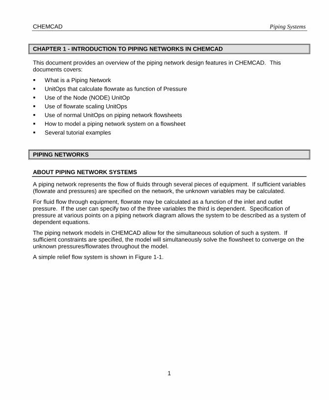
CHAPTER 1 - INTRODUCTION TO PIPING NETWORKS IN CHEMCAD
This document provides an overview of the piping network design features in CHEMCAD. This documents covers:
! What is a Piping Network ! UnitOps that calculate flowrate as function of Pressure ! Use of the Node (NODE) UnitOp ! Use of flowrate scaling UnitOps ! Use of normal UnitOps on piping network flowsheets ! How to model a piping network system on a flowsheet ! Several tutorial examples
PIPING NETWORKS
ABOUT PIPING NETWORK SYSTEMS
A piping network represents the flow of fluids through several pieces of equipment. If sufficient variables (flowrate and pressures) are specified on the network, the unknown variables may be calculated.
For fluid flow through equipment, flowrate may be calculated as a function of the inlet and outlet pressure. If the user can specify two of the three variables the third is dependent. Specification of pressure at various points on a piping network diagram allows the system to be described as a system of dependent equations.
The piping network models in CHEMCAD allow for the simultaneous solution of such a system. If sufficient constraints are specified, the model will simultaneously solve the flowsheet to converge on the unknown pressures/flowrates throughout the model.
A simple relief flow system is shown in Figure 1-1.

Piping Systems CHEMCAD
2
Figure 1-1: Simple Relief Flow
To size the valve, the pressure out of the valve must be calculated. Known variables are geometry of the pipe, pressure out of pipe, and flowrate through pipe. A single equation can be used to solve for the pressure into the pipe as a function of the known variables.
FLOWRATE AS A FUNCTION OF PRESSURE FOR FLUID FLOW
Fluid mechanics allows the calculation of fluid flowrate through a pipe or nozzle as a function of inlet and outlet pressures. The use of performance curves allows the calculation of fluid flow through a compressor or pump as a function of inlet and outlet pressures. Figure 1-2 shows UnitOps that may calculate flowrate as a function of pressures. These UnitOps are referred to as flow scaling UnitOps in this document because they scale the flowrate of the process stream.

CHEMCAD Piping Systems
3
Figure 1-2
ABOUT MODELING PIPING NETWORK SYSTEMS
Piping network systems are used to solve for flowrates and/or pressures around a network of connected equipment. Typically the user has a flowsheet of equipment connections and various constraints (exit flowrates, pressure limitations on equipment, etc.) but does not have all the flowrate(s) and/or pressure(s) for the system.
You may solve a piping network system on a CHEMCAD flowsheet. New models in CHEMCAD allow you to specify the known variables and solve for the unknown variables on a flowsheet.

Piping Systems CHEMCAD
4
The NODE UnitOp allows you to specify the pressure on either side of a UnitOp and calculate the flowrate as a function of pressure. As an option, you may specify one pressure and the flowrate. Iterative calculations will solve for the unknown pressure based on the specified pressure and flowrate. A series of UnitOps may be connected using several nodes. The flowrate through the chain may be specified at a single point, or calculated based on specified pressures around a UnitOp. It is not necessary to know the pressures around all UnitOps in the series.
Figure 1-3 shows a simple flare network. There are seven variables of pressure and flowrate. Three of the variables must be specified.
Figure 1-3

CHEMCAD Piping Systems
5
CHAPTER 2 – UNITOPS FOR PIPING NETWORKS
PRESSURE NODE
The piping network calculations solve for pressure at nodes and then iteratively calculate the flowrates through the network as functions of pressure.
A NODE UnitOp represents a point in the piping network where a change in pressure occurs due to elevation change, flow through a pipe, or flow through equipment that changes pressure (pump, valve, etc). A CHEMCAD flowsheet for a piping network uses the pipe UnitOp for piping effects and UnitOps such as the pump, compressor, and control valve.
For design of a piping network it is necessary to determine pressure between all UnitOps that calculate pressure as a function of flowrate. The NODE UnitOp sets the pressure on one side of a UnitOp that calculates pressure as a function of flowrate.
The pressure at a node may be specified by the user or calculated by CHEMCAD. The flowrate(s) in and out of a node may be specified or calculated. The flowrates may be specified at the NODE UnitOp, or calculated as dependent on adjacent UnitOps.
The NODE UnitOp sets a fixed value on the flowsheet. For piping network calculations there are points on the flowsheet where either the pressure or flowrate is known. The NODE UnitOp allows specification of the known variable and calculation of the unknown variable.
To learn the concepts for specifying a node, look at a system of two nodes surrounding a UnitOp. This is shown in Figure 2-1.

Piping Systems CHEMCAD
6
Figure 2-1
For the system in Figure 2-1 the inlet pressure (P1), outlet pressure (P2), and flowrate (F) through the pipe are the three variables. A single equation constrains the system. Specification of any two of the variables allows CHEMCAD to solve for the third variable.
If pressure is specified at the first node and either node specifies flowrate, the pressure of the second node is variable. CHEMCAD will vary the pressure of the second node until flowrate as a function of pressure around the pipe equals the specified flowrate. The pressure may vary at either node.
The pressure of a feed or product stream of known flowrate may be adjusted by adjacent nodes. In Figure 2-1, specifying P1 as fixed pressure specifies the pressure of stream 1 as P=P1.
If pressure at both nodes is specified, the flowrate through the UnitOp is a dependent variable. The variable flowrate may be either the feed stream or product stream. In the NODE UnitOp, specify the location where flowrate is a variable. Use mode free outlet or free inlet to specify whether the inlet or outlet flow is calculated. The model will cascade this flowrate upstream and downstream of the UnitOp.

CHEMCAD Piping Systems
7
The pressure of streams attached to a NODE UnitOp will be set to the pressure of the node. The flowrates through a network will all be set to the calculated flowrate through a node. You may specify N – 1 flowrates on a flowsheet, where N is the total of feed and product streams on the flowsheet. The calculated flowrate will be passed through nodes that use the dependent flowrate. You will receive an error message if you attempt to specify or calculate two conflicting flowrates through a system with two separate nodes.
Flowrate Options at Node
The flowrate for an inlet or outlet stream may be manipulated by a node. The node acts by manipulating the flowrate of the adjacent UnitOp. The pressure settings for the nodes on either side of the adjacent UnitOp contribute to the flowrate manipulation.
Fixed Flowrates at Node
Using a fixed inlet flowrate for a node specifies the flowrate through the upstream UnitOp. The pressure on one side (node) of the UnitOp must be variable. An exception is when a node is acting as a mixer or divider for N streams and the one stream is variable. In this situation the pressure can be fixed or variable for both nodes.
The Fixed outlet flowrate for a node specifies the flowrate through the downstream UnitOp. This setting is similar to fixed inlet.
The Current flowrate setting for an inlet stream is similar to fixed inlet. The current flowrate uses the flowrate currently stored for the inlet stream rather than a specified value in the node.
Variable Flowrates at Node
Using free inlet for a node specifies that the feed stream flowrate is a calculated variable. The node will manipulate the upstream feed flowrate to solve the system. The free inlet specification works best on a node connected to a Feed stream but it may be placed elsewhere on the flowsheet.
If the outlet flow is specified, the free inlet specification allows the feed to be calculated to maintain mass balance. Only one free inlet specification is allowed per feed stream.
The free outlet stream for a node is similar to the free inlet setting. Using free outlet specifies that the product stream flowrate is a calculated variable. The node will manipulate the product flowrate to solve the system. The free outlet specification works best on a node connected to a product stream but it may be placed elsewhere on the flowsheet.
If the inlet flow to a system is specified, the free outlet specification allows the product to be calculated to maintain mass balance. Only one free outlet specification is allowed per product stream.
If you attempt to specify too many free outlet or free inlet streams, CHEMCAD will issue a warning message and reset the extra specifications to flow set by UnitOp.
The flow set by UnitOp setting indicates that the flowrate is controlled by the adjacent UnitOp. The UnitOp may be calculating flowrate as a function of pressure. The UnitOp may be using the flowrate calculated by another UnitOp.

Piping Systems CHEMCAD
8
Mass Balance Limitations for Flowrate Calculation
Only one UnitOp on a branch of the network may calculate flowrate. If the nodes adjacent to a UnitOp both use flow set by UnitOp and fixed pressure, the calculated flowrate may be used as the flowrate at a free inlet or free outlet node. If the nodes adjacent to a UnitOp use flow set by UnitOp but do not both fix pressure, the flowrate through the UnitOp is calculated elsewhere on the flowsheet.
The behavior of Flow set by UnitOp depends on the flowrate specifications of other nodes on the branch. To illustrate, we consider a system from Figure 2-1.
The inlet to SECOND NODE is flow set by UnitOp.
The node will use the flowrate from the pipe.
If the feed stream is fixed inlet, this is the flowrate for the pipe.
If the feed stream is free inlet and the product streams are fixed flowrate, the free inlet feed flowrate is set by mass balance. The free inlet is the flow through the pipe. If the feed stream is free inlet, one product stream is free outlet, and both nodes are fixed pressure, the free inlet and free outlet are set by the pipe flowrate. The pipe flowrate is set to the critical flowrate for the given pipe with the specified inlet and outlet pressures.
The example job demonstrates various behaviors of flow settings for nodes. Figure 2-2 shows the flowsheet for this job.

CHEMCAD Piping Systems
9
Figure 2-2
NODE AS DIVIDER
A node may be used as a divider. Outlet streams from the node will be at the pressure of the node. Outlet streams will all have the same temperature and composition but flowrates may differ.
The flowrates may be specified as set by pipe/valve or fixed flowrates. Only one outlet stream flowrate may be free outlet.
A Node specified as a divider is shown in Figure 2-3. The second node acts as a divider (two product streams). For N inlet and outlet streams it is necessary to specify N-1 values.

Piping Systems CHEMCAD
10
For the second node in Figure 2-3, specify the flowrate of two of the three connected streams. Allow the third stream to be free for mass balance requirements.
Figure 2-3
If both outlet flowrates are specified, the inlet stream must be calculated as free inlet at node 1 to maintain mass balance. If one outlet is calculated as free outlet by the node, the inlet stream may be flow set by pipe if both nodes are fixed pressure.
PRESSURE NODE DIALOG SCREEN
Mode
Select Fixed pressure to set the pressure at the node and allow flowrate to be variable. Select Variable Pressure to leave pressure variable at the node.
CHEMCAD Piping Systems
11
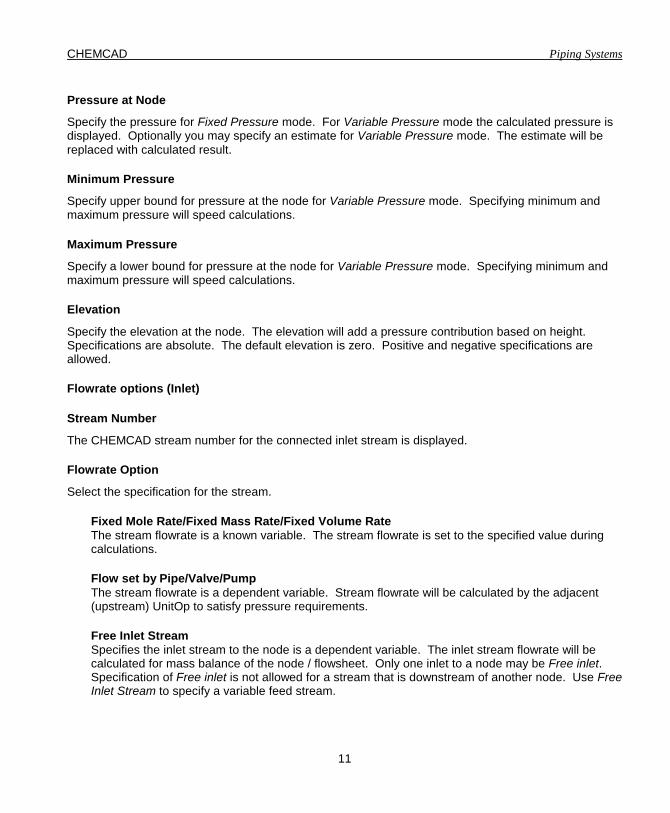
Pressure at Node
Specify the pressure for Fixed Pressure mode. For Variable Pressure mode the calculated pressure is displayed. Optionally you may specify an estimate for Variable Pressure mode. The estimate will be replaced with calculated result.
Minimum Pressure
Specify upper bound for pressure at the node for Variable Pressure mode. Specifying minimum and maximum pressure will speed calculations.
Maximum Pressure
Specify a lower bound for pressure at the node for Variable Pressure mode. Specifying minimum and maximum pressure will speed calculations.
Elevation
Specify the elevation at the node. The elevation will add a pressure contribution based on height. Specifications are absolute. The default elevation is zero. Positive and negative specifications are allowed.
Flowrate options (Inlet)
Stream Number
The CHEMCAD stream number for the connected inlet stream is displayed.
Flowrate Option
Select the specification for the stream.
Fixed Mole Rate/Fixed Mass Rate/Fixed Volume Rate The stream flowrate is a known variable. The stream flowrate is set to the specified value during calculations.
Flow set by Pipe/Valve/Pump The stream flowrate is a dependent variable. Stream flowrate will be calculated by the adjacent (upstream) UnitOp to satisfy pressure requirements.
Free Inlet Stream Specifies the inlet stream to the node is a dependent variable. The inlet stream flowrate will be calculated for mass balance of the node / flowsheet. Only one inlet to a node may be Free inlet. Specification of Free inlet is not allowed for a stream that is downstream of another node. Use Free Inlet Stream to specify a variable feed stream.
Piping Systems CHEMCAD
12
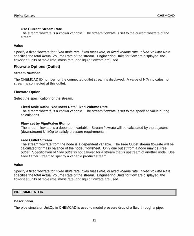
Use Current Stream Rate The stream flowrate is a known variable. The stream flowrate is set to the current flowrate of the stream.
Value
Specify a fixed flowrate for Fixed mole rate, fixed mass rate, or fixed volume rate. Fixed Volume Rate specifies the total Actual Volume Rate of the stream. Engineering Units for flow are displayed; the flowsheet units of mole rate, mass rate, and liquid flowrate are used.
Flowrate Options (Outlet) Stream Number
The CHEMCAD ID number for the connected outlet stream is displayed. A value of N/A indicates no stream is connected at this outlet.
Flowrate Option
Select the specification for the stream.
Fixed Mole Rate/Fixed Mass Rate/Fixed Volume Rate The stream flowrate is a known variable. The stream flowrate is set to the specified value during calculations.
Flow set by Pipe/Valve /Pump The stream flowrate is a dependent variable. Stream flowrate will be calculated by the adjacent (downstream) UnitOp to satisfy pressure requirements.
Free Outlet Stream The stream flowrate from the node is a dependent variable. The Free Outlet stream flowrate will be calculated for mass balance of the node / flowsheet. Only one outlet from a node may be Free outlet. Specification of Free outlet is not allowed for a stream that is upstream of another node. Use Free Outlet Stream to specify a variable product stream.
Value
Specify a fixed flowrate for Fixed mole rate, fixed mass rate, or fixed volume rate. Fixed Volume Rate specifies the total Actual Volume Rate of the stream. Engineering Units for flow are displayed; the flowsheet units of mole rate, mass rate, and liquid flowrate are used.
PIPE SIMULATOR
Description
The pipe simulator UnitOp in CHEMCAD is used to model pressure drop of a fluid through a pipe.
CHEMCAD Piping Systems
13
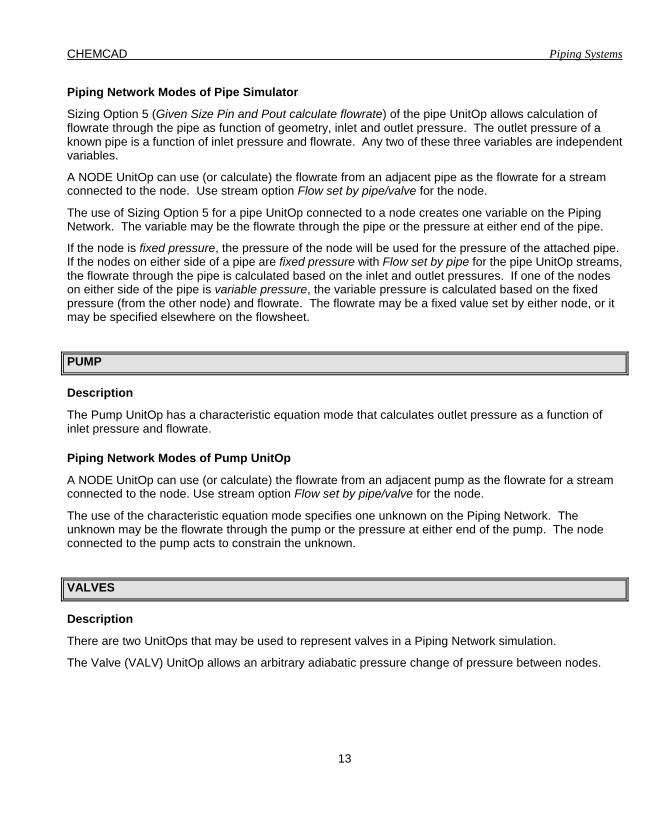
Piping Network Modes of Pipe Simulator
Sizing Option 5 (Given Size Pin and Pout calculate flowrate) of the pipe UnitOp allows calculation of flowrate through the pipe as function of geometry, inlet and outlet pressure. The outlet pressure of a known pipe is a function of inlet pressure and flowrate. Any two of these three variables are independent variables.
A NODE UnitOp can use (or calculate) the flowrate from an adjacent pipe as the flowrate for a stream connected to the node. Use stream option Flow set by pipe/valve for the node.
The use of Sizing Option 5 for a pipe UnitOp connected to a node creates one variable on the Piping Network. The variable may be the flowrate through the pipe or the pressure at either end of the pipe.
If the node is fixed pressure, the pressure of the node will be used for the pressure of the attached pipe. If the nodes on either side of a pipe are fixed pressure with Flow set by pipe for the pipe UnitOp streams, the flowrate through the pipe is calculated based on the inlet and outlet pressures. If one of the nodes on either side of the pipe is variable pressure, the variable pressure is calculated based on the fixed pressure (from the other node) and flowrate. The flowrate may be a fixed value set by either node, or it may be specified elsewhere on the flowsheet.
PUMP
Description
The Pump UnitOp has a characteristic equation mode that calculates outlet pressure as a function of inlet pressure and flowrate.
Piping Network Modes of Pump UnitOp
A NODE UnitOp can use (or calculate) the flowrate from an adjacent pump as the flowrate for a stream connected to the node. Use stream option Flow set by pipe/valve for the node.
The use of the characteristic equation mode specifies one unknown on the Piping Network. The unknown may be the flowrate through the pump or the pressure at either end of the pump. The node connected to the pump acts to constrain the unknown.
VALVES
Description
There are two UnitOps that may be used to represent valves in a Piping Network simulation.
The Valve (VALV) UnitOp allows an arbitrary adiabatic pressure change of pressure between nodes.
Piping Systems CHEMCAD
14
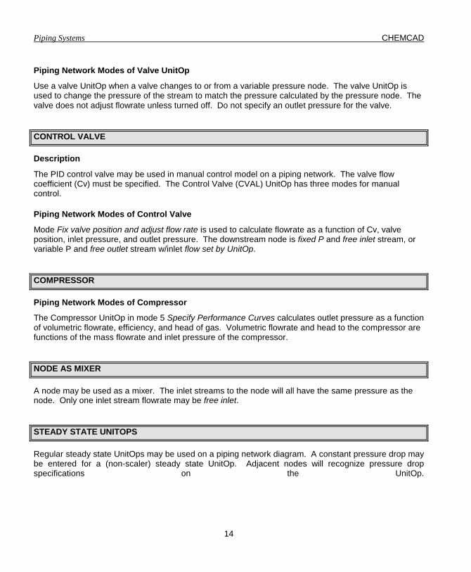
Piping Network Modes of Valve UnitOp
Use a valve UnitOp when a valve changes to or from a variable pressure node. The valve UnitOp is used to change the pressure of the stream to match the pressure calculated by the pressure node. The valve does not adjust flowrate unless turned off. Do not specify an outlet pressure for the valve.
CONTROL VALVE
Description
The PID control valve may be used in manual control model on a piping network. The valve flow coefficient (Cv) must be specified. The Control Valve (CVAL) UnitOp has three modes for manual control.
Piping Network Modes of Control Valve
Mode Fix valve position and adjust flow rate is used to calculate flowrate as a function of Cv, valve position, inlet pressure, and outlet pressure. The downstream node is fixed P and free inlet stream, or variable P and free outlet stream w/inlet flow set by UnitOp.
COMPRESSOR
Piping Network Modes of Compressor
The Compressor UnitOp in mode 5 Specify Performance Curves calculates outlet pressure as a function of volumetric flowrate, efficiency, and head of gas. Volumetric flowrate and head to the compressor are functions of the mass flowrate and inlet pressure of the compressor.
NODE AS MIXER
A node may be used as a mixer. The inlet streams to the node will all have the same pressure as the node. Only one inlet stream flowrate may be free inlet.
STEADY STATE UNITOPS
Regular steady state UnitOps may be used on a piping network diagram. A constant pressure drop may be entered for a (non-scaler) steady state UnitOp. Adjacent nodes will recognize pressure drop specifications on the UnitOp.

CHEMCAD Piping Systems
15
Between two nodes there must be one flowrate scaler. A heat exchanger and a pipe can be between two nodes, as the heat exchanger does not calculate flowrate as a function of pressure. A constant pressure drop may be specified for the heat exchanger and it will affect the pressure drop between the two nodes. A heat exchanger cannot be the only UnitOp between two nodes, as the heat exchanger does not have an effect on pressure.
CHAPTER 3 – CONTROL VALVE SIZING
Topics Covered
• Control Valve Sizing • Control Valve • Using Nodes
Problem Statement
The example is to size control valves for handling a flow of 113,000 lb/hr of Liquid Ammonia in each line coming from vessel D-1.
We wish to select appropriate sized valves and then determine the percent open for each valve at the rated service.
D-1-9F225 psig
D-2-1F15 psig
D-3-28F0.2 psig
This example is located in the CC5DATA\Examples\Piping\Example1 folder.

Piping Systems CHEMCAD
16
To size the valves using CHEMCAD, we have to convert the problem statement into a simulation. Let CHEMCAD calculate the properties for us, and then let CHEMCAD calculate the valve requirements.
The Simulation
To do the initial sizing, all we need are streams with the correct properties. It is not necessary to model the tanks:
11 2
3
In the flowsheet shown above, all three streams are at the inlet conditions of -9 degrees F, 225 psig. The divider splits the 226,000 lb/hr flow into 2 equal flows of 113,000 lb/hr of ammonia.
Control Valve Sizing
To do the initial sizing, run the simulation (Run menu>Run All) to calculate the flow information for streams 2 and 3. Both streams should be at -9 degrees F, 225 psig and 113,000 lb/hr of ammonia.
Next select stream 2 by left clicking on it. The stream is selected when it is shown bracketed by black squares. Go to the Sizing menu, and select Control valve. The following screen will appear:

CHEMCAD Piping Systems
17
Enter 15 psig as the Downstream pressure and press the OK button. On the screen will appear the following report:
CHEMCAD reports the properties of the stream, and the calculated parameters for the valve. We repeat the procedure for stream 3:

Piping Systems CHEMCAD
18
In the next section we will rate these valves to see what their performance is in this service.
Rating Case
Our next task is to rate these valves in a simulation. We want to know what the percent open is for these valves in this service at 113,000 lb/hr. Since this task models the behavior of the control valves we will need a slightly larger flowsheet:

CHEMCAD Piping Systems
19
1
2
3
1
4
5
6
7
4
8
3
5
9
2
The flash UnitOps at the end aren’t necessary, they are included so we could see our vapor and liquid flowrates in separate streams if flashing occurs.
The divider is still set to 113,000 lb/hr and the flash tanks are set to mode 2 (specify T and P) Flash UnitOp #2 is set to -1 degrees F, 15 psig and Flash UnitOp #3 is set to -28 degrees F,0 .2 psig.
Open the control valve #4 by double-clicking on it. The control valve screen is shown below:

Piping Systems CHEMCAD
20
Enter the Valve flow coefficient of 36, the Downstream pressure to 15 psig, and set the Valve mode setting to Fix flow rate, adjust valve position. Press OK and move on to Valve #5. Valve #5 is set in the same way, with a Valve flow coefficient of 54, Downstream pressure of 0.2 psig, and Valve mode set to fix flow rate, adjust valve position.
Run the simulation by going to the Run menu and selecting Run All. To view your results, go to the Results menu, and select UnitOp’s. You should see this dialog asking for what UnitOps to view:
If you don’t see this, then you already have a unit selected in the flowsheet, and it is showing you a report for that unit. Close the report, deselect the UnitOps by holding down the shift key while clicking on
CHEMCAD Piping Systems
21
the units, and go back to Results, UnitOp’s. You can also deselect UnitOps by left-clicking on a blank section of the worksheet.
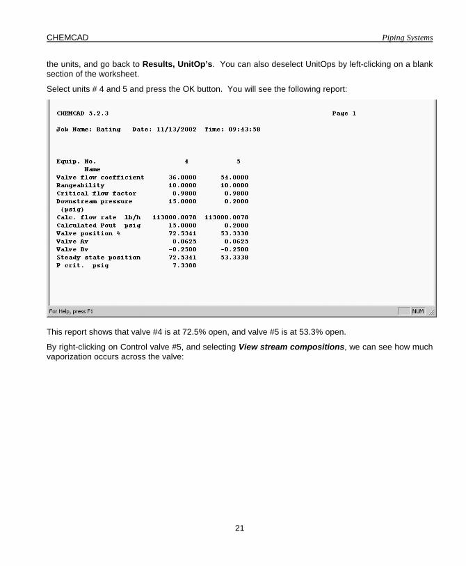
Select units # 4 and 5 and press the OK button. You will see the following report:
This report shows that valve #4 is at 72.5% open, and valve #5 is at 53.3% open.
By right-clicking on Control valve #5, and selecting View stream compositions, we can see how much vaporization occurs across the valve:

Piping Systems CHEMCAD
22
This volume change is why CHEMCAD chose a larger valve for the second stream. With the vaporization occurring in the valve, a smaller 2-inch valve body would be approaching sonic velocity through the valve body.
Flowrate as a function of Pressure
In typical CHEMCAD simulations information flows in one direction: downstream. Upstream conditions determine the downstream conditions. In most simulations, you simply set the flowrates and pressures of feed streams. Pressure drops are either calculated based on flow or specified through UnitOps. The downstream pressures, flowrates, etc. are calculated when the simulation is run.
For piping simulations, flowrate and pressure are dependent on each other. The backpressure on valves, pipes, and other UnitOps affects the flowrate through the valve. Likewise, the flowrate through a valve, (or pipe, or pump) determines the downstream pressure.
In flow models like the control valve sizing model, sometimes it is useful to let flowrate vary as a function of the pressure.
For example, assume a process upset caused the pressure in vessel D-2 to rise from 15 psig to 30 psig. Assuming the valve positions don’t change, what is the new flowrate from D-1?

CHEMCAD Piping Systems
23
D-1-9 F225 psig
D-2-1 F30 psig (UPSET condition)
D-3-28F0.2 psig
Cv=3672.5 % open
Cv=5453.3% open
In order to answer this question, we need to introduce a special UnitOp called a node. A node is a point in the simulation that has a pressure, flow coming in, and flow going out. The node units create a network, solving for flowrate at each point based on the fixed pressures. Nodes are placed on the flowsheet before and after the control valves. For our system, the flowsheet is shown below:
6 7
8
9
10
10 11
12
13
14
11
15
18
12
16
19
20
17
The function of the divider (to split the incoming flow) is now handled by NODE #6. The node will balance the flowrates such that all streams entering and exiting the node are at the same pressure. Nodes are also placed between the flash vessels and the control valves. At the nodes we can fix the pressures, and let the flowrate vary as a function of valve position and pressure difference.
Open NODE #6 by double-clicking on it:

Piping Systems CHEMCAD
24
We are assuming the pressure at this node is fixed at 225 psig. The inlet flow is set to Free inlet stream and the two outlet streams are set to Flow set by UnitOp. Flow into each control valve will be determined by the control valve Cv valve opening position, and pressure difference across the valve.
The other two NODE UnitOps are set in a similar fashion.

CHEMCAD Piping Systems
25
The pressure in is set to 30 psig for NODE #9, 0.2 psig for NODE #10. Flow into the node is controlled by the control valve (Flow set by UnitOp), flow out is a Free Outlet Stream.
The control valves need to be changed to fix the valve position, and calculate flowrate.
Piping Systems CHEMCAD
26
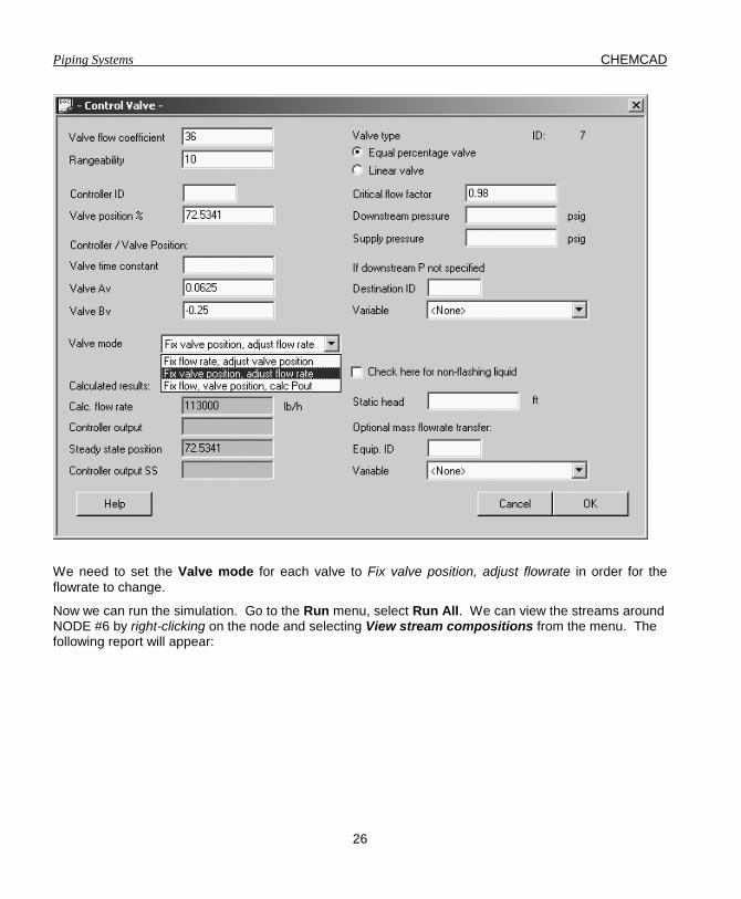
We need to set the Valve mode for each valve to Fix valve position, adjust flowrate in order for the flowrate to change.
Now we can run the simulation. Go to the Run menu, select Run All. We can view the streams around NODE #6 by right-clicking on the node and selecting View stream compositions from the menu. The following report will appear:

CHEMCAD Piping Systems
27
The flowrate from D-1 to D-2 dropped from 113,000 lb/hr to 109138 lb/hr. So we can see the effect of back pressure on the flowrates through the valves.
CHAPTER 4 �SIMPLE FLOW EXAMPLE
Topics Covered
• Control Valve Sizing • Feedback Controllers • NPSH • Orifice Sizing/Rating • Pipe Sizing/Rating • Pipe UnitOp
Problem Statement
The piping system shown must be designed to transport 120 gpm of glacial acetic acid at 70-140F. The pressure at the inlet is known at 20 psia, the outlet must be no less than 20psia. The piping system and its individual elements must be sized for design conditions and then rated at operating conditions. Our goal is to determine the NPSHa and head requirements for future pump selection.
Piping Systems CHEMCAD
28
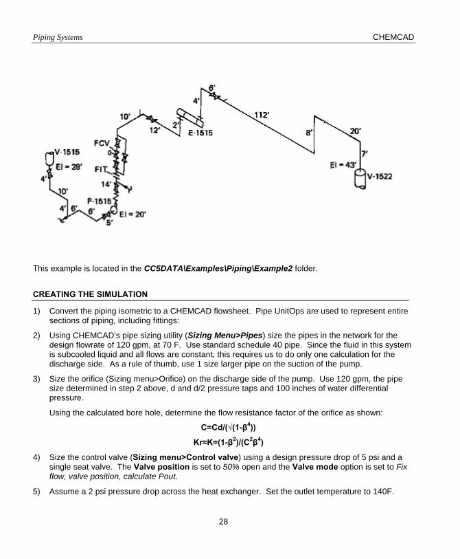
This example is located in the CC5DATA\Examples\Piping\Example2 folder.
CREATING THE SIMULATION
1) Convert the piping isometric to a CHEMCAD flowsheet. Pipe UnitOps are used to represent entire sections of piping, including fittings:
2) Using CHEMCAD’s pipe sizing utility (Sizing Menu>Pipes) size the pipes in the network for the design flowrate of 120 gpm, at 70 F. Use standard schedule 40 pipe. Since the fluid in this system is subcooled liquid and all flows are constant, this requires us to do only one calculation for the discharge side. As a rule of thumb, use 1 size larger pipe on the suction of the pump.
3) Size the orifice (Sizing menu>Orifice) on the discharge side of the pump. Use 120 gpm, the pipe size determined in step 2 above, d and d/2 pressure taps and 100 inches of water differential pressure.
Using the calculated bore hole, determine the flow resistance factor of the orifice as shown:
C=Cd/(√(1-β4))
Kr≈K=(1-β2)/(C2β4)
4) Size the control valve (Sizing menu>Control valve) using a design pressure drop of 5 psi and a single seat valve. The Valve position is set to 50% open and the Valve mode option is set to Fix flow, valve position, calculate Pout.
5) Assume a 2 psi pressure drop across the heat exchanger. Set the outlet temperature to 140F.
CHEMCAD Piping Systems
29
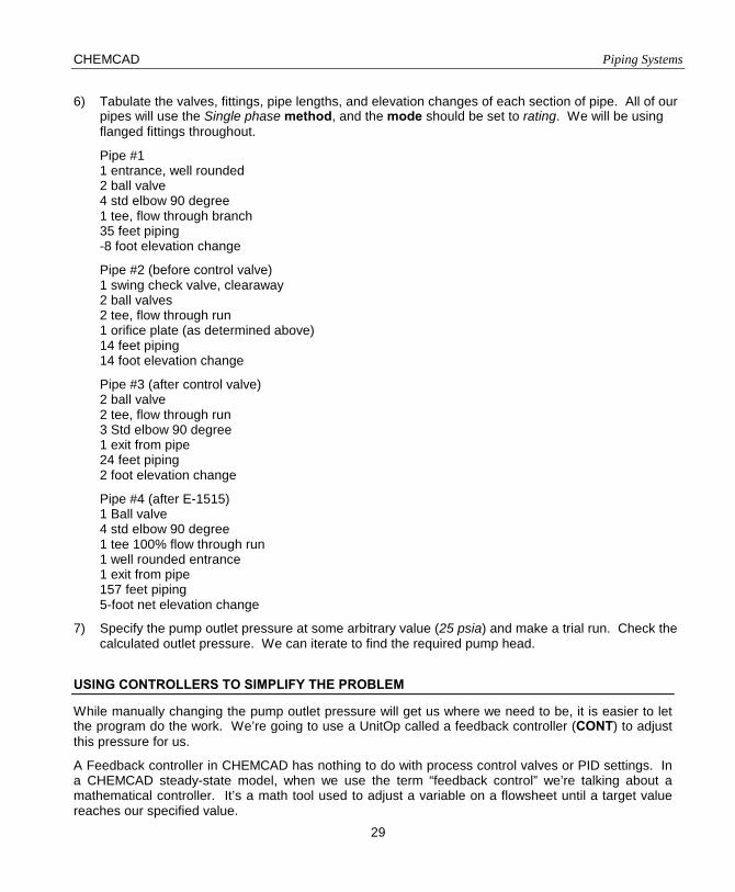
6) Tabulate the valves, fittings, pipe lengths, and elevation changes of each section of pipe. All of our pipes will use the Single phase method, and the mode should be set to rating. We will be using flanged fittings throughout.
Pipe #1 1 entrance, well rounded 2 ball valve 4 std elbow 90 degree 1 tee, flow through branch 35 feet piping -8 foot elevation change
Pipe #2 (before control valve) 1 swing check valve, clearaway 2 ball valves 2 tee, flow through run 1 orifice plate (as determined above) 14 feet piping 14 foot elevation change
Pipe #3 (after control valve) 2 ball valve 2 tee, flow through run 3 Std elbow 90 degree 1 exit from pipe 24 feet piping 2 foot elevation change
Pipe #4 (after E-1515) 1 Ball valve 4 std elbow 90 degree 1 tee 100% flow through run 1 well rounded entrance 1 exit from pipe 157 feet piping 5-foot net elevation change
7) Specify the pump outlet pressure at some arbitrary value (25 psia) and make a trial run. Check the calculated outlet pressure. We can iterate to find the required pump head.
USING CONTROLLERS TO SIMPLIFY THE PROBLEM
While manually changing the pump outlet pressure will get us where we need to be, it is easier to let the program do the work. We’re going to use a UnitOp called a feedback controller (CONT) to adjust this pressure for us.
A Feedback controller in CHEMCAD has nothing to do with process control valves or PID settings. In a CHEMCAD steady-state model, when we use the term “feedback control” we’re talking about a mathematical controller. It’s a math tool used to adjust a variable on a flowsheet until a target value reaches our specified value.

Piping Systems CHEMCAD
30
Change the flowsheet to include a feedback controller just before the product arrow:
1 23 4 5 6 71
2 34
56
7 8
8 9
Specify the Controller mode as a feedback controller. Adjust pump outlet pressure until the pressure of stream 8 is equal to a constant target of 20 psia. When you are finished, the controller screen should look like so:
When you run the simulation, the controller will automatically change the pump outlet pressure until the pressure leaving the last pipe unit is equal to 20. We now know the head requirements for our pump.

CHEMCAD Piping Systems
31
CALCULATING NPSHA
NPSH is the Net Positive Suction Head, and it is defined as the total pressure available at the pump suction minus the pumping fluids vapor pressure. It is almost always reported in feet of pumped fluid or water.
Every pump has a specified NPSH requirement (NPSHr) at a given operating speed. To ensure reliable operation the available NPSH (NPSHa) must be greater than the NPSHr. If not, cavitation and shortened service life may result.
Calculate NPSHa. The net positive suction head is defined as pressure available at pump suction minus the fluid vapor pressure, expressed in feet of fluid. To calculate this in CHEMCAD is an easy task. Open the Pump dialog, and put a checkmark where it says Check here to Calculate NPSHa. Rerun the simulation, and the calculated NPSHa will appear.
It is important to the NPSHa calculation that the inlet piping to the pump be correctly specified. If the piping is not correct, then the pressure at the inlet may not be correct, and the NPSHa may not be correct.
CHAPTER 5 –BRANCHED FLOW EXAMPLE
Topics Covered
• Node UnitOp • Pipe Networks • Pump Selection Criteria • Pump UnitOp Performance Curves
Problem Statement
The piping system from the previous section has been changed. Due to the branched flow to the two heat exchangers, the problem is no longer a simple one.

Piping Systems CHEMCAD
32
This example is located in the CC5DATA\Examples\Piping\Example3 folder.
The branched flow is a difficult problem to solve using our controller approach. The two exchangers have different piping, which gives them different flowrates. What we need is an approach where we split and recombine flows, and have the simulation calculate the pressure and flowrates in an iterative manner. The “node” UnitOp gives us this flexibility.
A node is a point where pressure is uniform. There may be multiple inlets and outlets. The flowrates for each stream will be balanced by CHEMCAD to reach a single pressure. Pressure may be specified or allowed to vary.
CREATING THE SIMULATION
1) Convert the piping isometric to a CHEMCAD flowsheet:

CHEMCAD Piping Systems
33
12
4
5
6
7
9 10 13 14
1 2
11
16
17 18 19
12
20
15 3
21
3
4
5
6
2019
1817
1615
14
1312
1110
9
8
7
8
22
2) Pipe UnitOps are used to represent entire sections of piping, including fittings. NODE UnitOps are
placed where pressure or flowrate are unknown.
3) Assume a 2 psi pressure drop across each heat exchanger.
4) Tabulate the valves, fittings, pipe lengths, and elevation changes of each section of pipe. We will be using flanged fittings throughout.
Pipe #1 1 entrance, well rounded 2 ball valve 4 std elbow 90 degree 1 tee, flow through branch 35 feet piping
Pipe #2 (before control valve) 1 swing check valve, clearaway 2 ball valves 2 tee, flow through run 1 orifice plate (as determined above) 14 feet piping
Piping Systems CHEMCAD
34
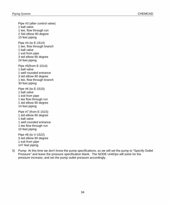
Pipe #3 (after control valve) 1 ball valve 1 tee, flow through run 2 Std elbow 90 degree 10 feet piping
Pipe #4 (to E-1514) 1 tee, flow through branch 1 ball valve 1 exit from pipe 3 std elbow 90 degree 24 feet piping
Pipe #5(from E-1514) 1 ball valve 1 well rounded entrance 3 std elbow 90 degree 1 tee, flow through branch 30 feet piping
Pipe #6 (to E-1515) 1 ball valve 1 exit from pipe 1 tee flow through run 1 std elbow 90 degree 14 feet piping
Pipe #7 (from E-1515) 1 std elbow 90 degree 1 ball valve 1 well rounded entrance 1 tee flow through run 10 feet piping
Pipe #8 (to V-1522) 3 std elbow 90 degree 1 exit from pipe 147 feet piping
5) Pump- At this time we don’t know the pump specifications, so we will set the pump to “Specify Outlet Pressure” and leave the pressure specification blank. The NODE UnitOps will solve for the pressure increase, and set the pump outlet pressure accordingly.
CHEMCAD Piping Systems
35
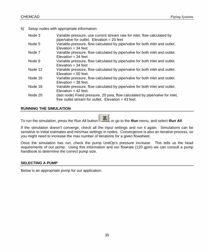
6) Setup nodes with appropriate information:
Node 3 Variable pressure, use current stream rate for inlet, flow calculated by pipe/valve for outlet. Elevation = 20 feet
Node 5 Variable pressure, flow calculated by pipe/valve for both inlet and outlet. Elevation = 34 feet
Node 7 Variable pressure, flow calculated by pipe/valve for both inlet and outlet. Elevation = 34 feet
Node 9 Variable pressure, flow calculated by pipe/valve for both inlet and outlet. Elevation = 34 feet
Node 12 Variable pressure, flow calculated by pipe/valve for both inlet and outlet. Elevation = 50 feet.
Node 16 Variable pressure, flow calculated by pipe/valve for both inlet and outlet. Elevation = 38 feet.
Node 18 Variable pressure, flow calculated by pipe/valve for both inlet and outlet. Elevation = 42 feet.
Node 20 (last node) Fixed pressure, 20 psia, flow calculated by pipe/valve for inlet, free outlet stream for outlet. Elevation = 43 feet.
RUNNING THE SIMULATION
To run the simulation, press the Run All button or go to the Run menu, and select Run All.
If the simulation doesn’t converge, check all the input settings and run it again. Simulations can be sensitive to initial estimates and min/max settings in nodes. Convergence is also an iterative process, so you might need to increase the max number of iterations for a given flowsheet.
Once the simulation has run, check the pump UnitOp’s pressure increase. This tells us the head requirements of our pump. Using this information and our flowrate (120 gpm) we can consult a pump handbook to determine the correct pump size.
SELECTING A PUMP
Below is an appropriate pump for our application.

Piping Systems CHEMCAD
36
Pump Curve
1750 rpm
1450 rpm
1150 rpm
2030405060708090
0 40 80 120 160 200
Flow (gpm)
Head
(ft)
1750 rpm1450 rpm
1150 rpm
0.3
0.35
0.4
0.45
0.5
0.55
0.6
0 40 80 120 160 200
Flow (gpm)
Effic
ienc
y
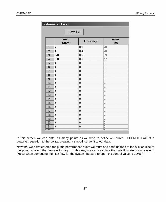
To enter this curve into our pump, select Specify Performance Curve for the pump Mode. Once you do you have the opportunity to enter multiple speed lines and an operating speed. For our purposes, we’ll assume we want the pump to be at 1750 RPM, so we enter a single speed line. Press the OK button, and you will see the following entry screen:
CHEMCAD Piping Systems
37
In this screen we can enter as many points as we wish to define our curve. CHEMCAD will fit a quadratic equation to the points, creating a smooth curve fit to our data.
Now that we have entered the pump performance curve we must add node unitops to the suction side of the pump to allow the flowrate to vary. In this way we can calculate the max flowrate of our system. (Note: when computing the max flow for the system, be sure to open the control valve to 100%.)

Piping Systems CHEMCAD
38
CHAPTER 6 - FLOW RELIEF PIPING SYSTEM
Topics Covered
• Branched Network • Compressible flow • Degrees of Freedom • Flare header systems • Node UnitOp • Pipe UnitOp • Valve UnitOp
FLARE HEADER DESIGN
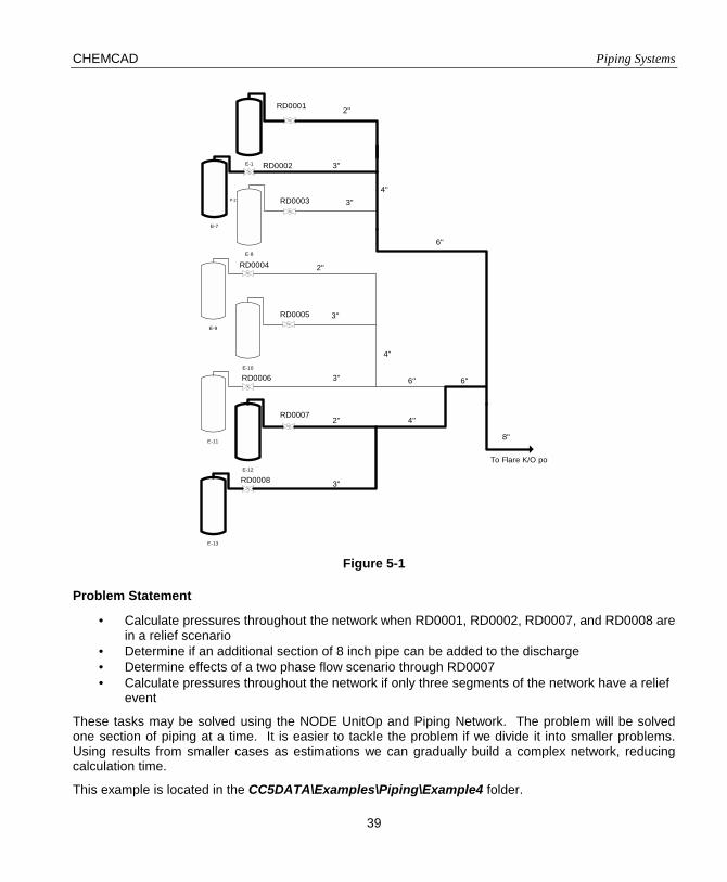
Flare headers are specialized piping networks desiged to convey relief valve flow to a flare where products are consumed before release to the atmosphere. Using CHEMCAD, we can design and evaluate flare header networks for many relieving scenarios.
Figure 5-1 shows a simplified flowsheet for a relief header network. The flows and pressures from relief devices RD0001-RD0008 are previously calculated. The piping network has been designed but not certified or built. The pipes on this flow diagram represent continuous sections of pipe with various fittings (elbows, etc).
CHEMCAD Piping Systems
39
E-1
E-7
P-2
E-8
E-9
E-10
E-11
E-12
E-13
RD0001
RD0002
RD0003
RD0004
RD0005
RD0006
RD0007
RD0008
2"
3"
4"3"
6"
2"
3"
4"
3" 6" 6"
8"
2"
3"
4"
To Flare K/O pot
Figure 5-1
Problem Statement
• Calculate pressures throughout the network when RD0001, RD0002, RD0007, and RD0008 are in a relief scenario
• Determine if an additional section of 8 inch pipe can be added to the discharge • Determine effects of a two phase flow scenario through RD0007 • Calculate pressures throughout the network if only three segments of the network have a relief
event
These tasks may be solved using the NODE UnitOp and Piping Network. The problem will be solved one section of piping at a time. It is easier to tackle the problem if we divide it into smaller problems. Using results from smaller cases as estimations we can gradually build a complex network, reducing calculation time.
This example is located in the CC5DATA\Examples\Piping\Example4 folder.
Piping Systems CHEMCAD
40
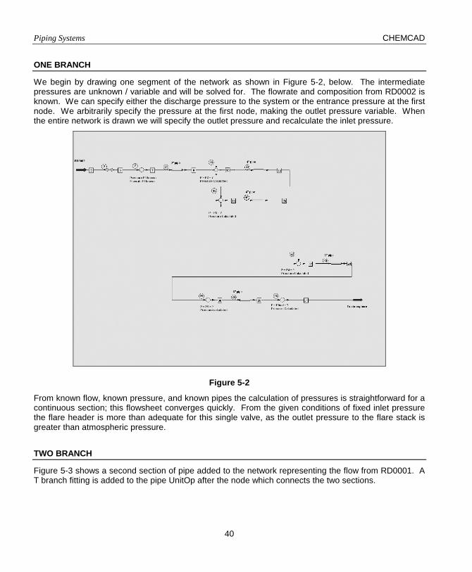
ONE BRANCH
We begin by drawing one segment of the network as shown in Figure 5-2, below. The intermediate pressures are unknown / variable and will be solved for. The flowrate and composition from RD0002 is known. We can specify either the discharge pressure to the system or the entrance pressure at the first node. We arbitrarily specify the pressure at the first node, making the outlet pressure variable. When the entire network is drawn we will specify the outlet pressure and recalculate the inlet pressure.
Figure 5-2
From known flow, known pressure, and known pipes the calculation of pressures is straightforward for a continuous section; this flowsheet converges quickly. From the given conditions of fixed inlet pressure the flare header is more than adequate for this single valve, as the outlet pressure to the flare stack is greater than atmospheric pressure.
TWO BRANCH
Figure 5-3 shows a second section of pipe added to the network representing the flow from RD0001. A T branch fitting is added to the pipe UnitOp after the node which connects the two sections.

CHEMCAD Piping Systems
41
Figure 5-3
The flowrate from RD0001 is known. The pressure at the first node for RD0001 is variable. If we consider the RD0001 section a separate section of pipe, we do not have a degree of freedom to specify. The pressure at the node where RD0001 flow combines with the RD0002 flow is a dependent variable for RD0001 flow; it is calculated by the RD0002 section.
FOUR BRANCH
A third and fourth branch are added to the network, shown in Figure 5-4 and Figure 5-5, below. As our flowsheet becomes more complex, the upper/lower bounds for pressure in nodes become more important. A more complex network may require more careful settings of upper and lower bounds.

Piping Systems CHEMCAD
42
Figure 5-4
Figure 5-5
The flowsheet is run and converged after adding the third and fourth sections. All four branches are on the network. The calculated discharge pressure is above atmospheric; the network is adequate for this relieving scenario.

CHEMCAD Piping Systems
43
SPECIFYING THE OUTLET PRESSURE
We can now perform a rating case on this network, to determine the minimum pressure at RD0002 for relief under this scenario.
The pressure on the first section node is changed to variable pressure. The outlet pressure for the network is changed to fixed pressure. The boundaries on variable pressures are tightened and the flowsheet is converged to the same results, but with the fixed pressure node changed from inlet to outlet.
To drop the pressure to 2 psig, one should relax the lower pressure boundaries on variable nodes. By making several minor adjustments from the current pressure to 2 psig, fewer calculations will be required.
ADDITION OF PIPE TO DISCHARGE
A pipe is added to the discharge of the network. The pipe is set to rating mode in CHEMCAD; there is no need to use nodes around this final pipe. The flowsheet is run, the final pipe calculates outlet pressure. The design modes of the pipe can be used to determine a required diameter for the pipe if the required length of pipe is known.
Figure 5-6
EFFECT OF CLOSED VALVE
The simple valve (VALV) UnitOp in CHEMCAD has a closed setting. This can be used to shutoff the flow to a section of pipe. In this example we set the valve on RD001 to closed and run the process.
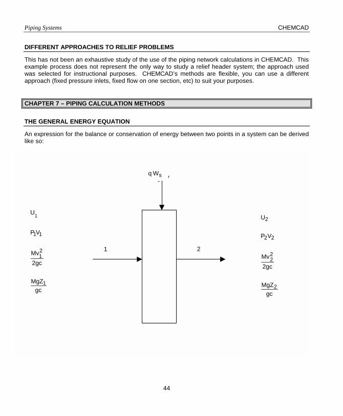
Piping Systems CHEMCAD
44
DIFFERENT APPROACHES TO RELIEF PROBLEMS
This has not been an exhaustive study of the use of the piping network calculations in CHEMCAD. This example process does not represent the only way to study a relief header system; the approach used was selected for instructional purposes. CHEMCAD’s methods are flexible, you can use a different approach (fixed pressure inlets, fixed flow on one section, etc) to suit your purposes.
CHAPTER 7 – PIPING CALCULATION METHODS
THE GENERAL ENERGY EQUATION
An expression for the balance or conservation of energy between two points in a system can be derived like so:
Qov
s Wq
1 2
gcMgZ
2gcMv
VP
U
1
21
11
1
gcMgZ
2gcMv
VP
U
2
22
22
2
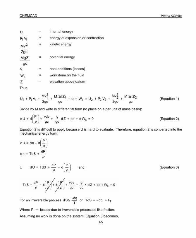
CHEMCAD Piping Systems
45
iU = internal energy
ii VP = energy of expansion or contraction
2gcMv2
i = kinetic energy
gcZMg i
= potential energy
q = heat additions (losses)
sW = work done on the fluid
Z = elevation above datum
Thus,
gcZgM
2gcMv
VPUWqgc
ZgM2gcMv
VPU 222
222s1
21
111⋅⋅+++=++⋅⋅+++ (Equation 1)
Divide by M and write in differential form (to place on a per unit of mass basis):
0WddqZdgcg
gcvdvPdUd s =++++
+
ρ (Equation 2)
Equation 2 is difficult to apply because U is hard to evaluate. Therefore, equation 2 is converted into the mechanical energy form.
ρ
ρdPTdShd
Pd-hdUd
+=
=
and;PddPTdSUd
−+=∴
ρρ (Equation 3)
For an irreversible process fP dq-TdSorT
-dqSd +=≥
Where Pf = losses due to irreversible processes like friction.
Assuming no work is done on the system; Equation 3 becomes,
0WddqZdgcg
gcvdvPdPddPTdS s =+•++
/
//+
/
//−+ρρρ

Piping Systems CHEMCAD
46
( )
0dPZ dgcg
gcvdvdP
00qdZdgcg
gcvdvdPqdP d
f
f
=+++
=+//++++//−+
ρ
ρ (Equation 4)
Z = dPf sin Φ = some angle of elevation
0dP sinLdgcg
gcvdvdp
f =+•++ φρ
(Equation 5)
Multiplying by L d
ρ
0dLdP sin
gcg
dLdv
gcv
dLdp f =+••+•+ ρφρρ (Equation 6)
CONSERVATION OF MOMENTUM
Conservation of Linear Momentum �
( ) o sinAd
LdPdv
Lddv
Ldd
g2 ρπτρρ −−−=
+•
where LdPd
= pressure loss
ADπτ
= shear stress loss (friction)
o singρ = gravitational loss
At steady state
o sinAD
LdPd
Ld
vdg
2
ρπτρ
−−=
( )Ldvdv
L dvdv
Ld
vd 2
•+=
ρρρ
( ) o sin
AD
LdPd
Ldvdv
Ldvdv gρπτρρ
−−=+

CHEMCAD Piping Systems
47
( ) o sinAD
dLdvv
Ldvdv
LdPd
gρπτρρ +++=
at steady state ( )
;0Ldvd
=ρ
and
o sinAD
Ldvdv
LdPd
gρπτρ ++= (Equation 7)
where
Ldvdvρ
= acceleration losses. Normally negligible and significant only if compressible flow exits at low pressure.
ADπτ
= friction losses
o singρ = hydrostatic head or elevation changes
Evaluation of wall shear stress (or friction losses) can be accomplished by defining a dimensionless friction factor,
Fanning friction factor volume /unitfluid the ofenergy kinetic
stress shear wall
2vf
2w =
=ρ
τ
Manipulation produces
( )equation Wiesbach-Darcy theD2vf
4DD
8vf
dLdP 2
2
2
f
ρπ
πρ =
=
(Equation 8)
FRICTION FACTOR DETERMINATION
For Laminar Flow an analytical expression can be derived for the friction factor
Re64f =
For Turbulent flow,the friction factor is developed from Colebrook
2
vfRe7.18
D2 Log274.1f :Colebrook
−
+−= ρ

Piping Systems CHEMCAD
48
In terms of a Darcy-Wiesbach or Moody friction factor, 4f'fm •= and Dg2
vfdLdP
c
2m
f
••=
ρ
ACCELERATION COMPONENT
1) Is zero for constant area, incompressible flow
2) For any flow condition in which a velocity change occurs, such as compressible flow, a pressure drop will occur in the direction of velocity increase.
THE ISOTHERMAL FLOW EQUATION The isothermal flow equation is solved as follows:
Nomenclature:
P1 = initial gas pressure, psia
P2 = terminal gas pressure, psia
D = terminal gas pressure, psia
L = pipe length, ft.
W = gas flow, lb/h
ρ = gas density, lb/ft3
MW = molecular weight of gas
P = gas pressure, psia
f = friction factor
R = gas constant, 10.73
T = absolute, temperature oR
( )
( )( )( )
RTPMW
1337.024D
PWPP
2lnD/f12LPP
P
PP
P/Pln2/DLf12D
1337.024W
05
24
12
2
1212
05
1
22
21
21
4
=
+−=
−
+=
ρ
ρ
ρ

CHEMCAD Piping Systems
49
THE DARCY-WEISBACH EQUATION
D(2gc)144fLvP
2ρ=∆
where, ∆P = pressure drop
ρ = density
f = friction factor
L = equivalent length
v = velocity
D = diameter
gc = gravitational constant
THE HAZEN-WILLIAMS EQUATION
The Hazen-Williams equation is used for the design of water sprinkler systems for fire protection. It�s use is mandated by the National Fire Protection Association the designer of such systems.
The Hazen and Williams formula for flow of water is:
54.0212.63
LPPCD0.442Q
−=
where, C = 140 for new steel pipe
C = 130 for new cast iron pipe
C = 100 is often used for design purposes to account for pipe fouling etc.
and, Q = volumetric flow of water, gal/min
D = inside diameter, ft
P = pressure, psia
L = length of pipe segment, ft
THE FRITZCHE EQUATION
The Fritzche equation is used to calculate the pressure drops in steam systems.
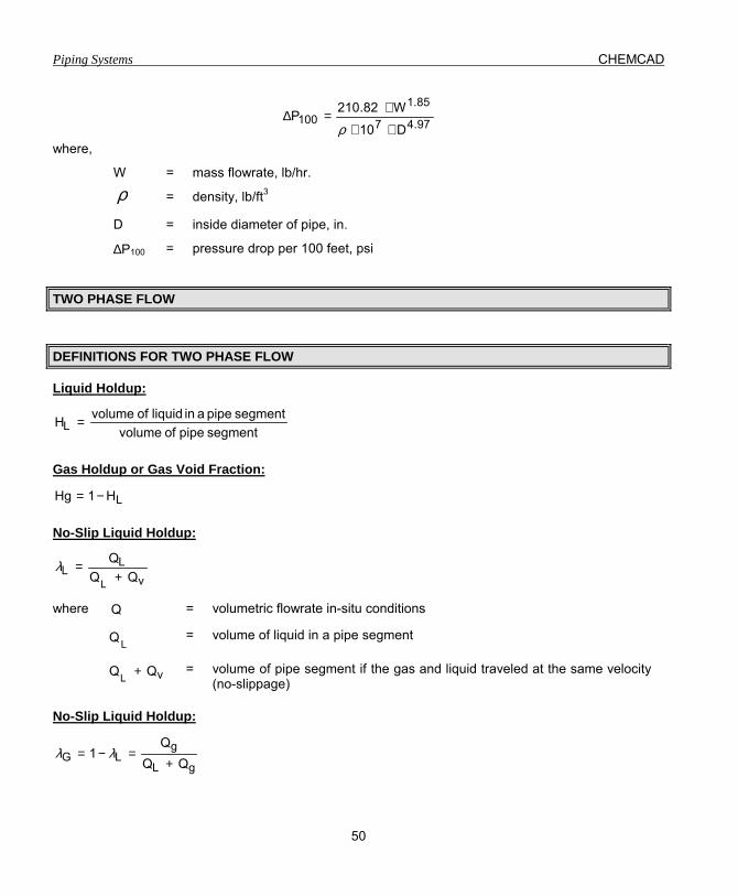
Piping Systems CHEMCAD
50
97.47
85.1100
D10
W82.210P∗∗
∗=∆ρ
where,
W = mass flowrate, lb/hr.
ρ = density, lb/ft3
D = inside diameter of pipe, in.
∆P100 = pressure drop per 100 feet, psi
TWO PHASE FLOW
DEFINITIONS FOR TWO PHASE FLOW
Liquid Holdup:
segment pipe of volumesegment pipe a in liquid of volumeHL =
Gas Holdup or Gas Void Fraction:
LH1Hg −=
No-Slip Liquid Holdup:
vL
L QQQ
L +=λ
where Q = volumetric flowrate in-situ conditions
LQ = volume of liquid in a pipe segment
vQQL + = volume of pipe segment if the gas and liquid traveled at the same velocity (no-slippage)
No-Slip Liquid Holdup:
gL
gLG QQ
Q1
+=−= λλ

CHEMCAD Piping Systems
51
Two-Phase Density:
Calculation of the two-phase density requires knowledge of the liquid holdup, 3 equations used:
ggLLs HH ρρρ +=
ggLLn λρλρρ +=
g
2gg
L
2LL
k HHλρλρ
ρ +=
Superficial Velocity:
The velocity which that phase would exhibit if it flowed through the total cross section of the pipe above.
Superficial gas velocity = sgv =
AQg
Superficial liquid velocity = Slv =
AQL
Superficial two phase velocity = Mv = sgSl vv +
SLIP VELOCITY:
The difference in the actual gas and liquid velocities, sV :
lsl
g
sgLgS H
vHv
vvv −=−=
Therefore, Msl
L vv=λ
MODIFICATION OF THE PRESSURE GRADIENT EQUATION FOR TWO PHASE FLOW
Assume that the gas-liquid mixture can be considered homogeneous over a finite volume of pipe,
The Elevation Component = o singcg
dLdP
sl
••=
ρ where llggs HH ρρρ += .

Piping Systems CHEMCAD
52
The Friction Loss Component = d2g
vfdLdP
c
2Mftp
f
••=
ρ
The Acceleration Component = ignored. frequentlydLdP
acc=
THE BAKER METHOD FOR TWO PHASE FLOW CALCULATIONS
Establishing the Two-Phase Flow Pattern:
CHEMCAD establishes the two-phase flow pattern by using the following Baker Chart (this chart is accurate for horizontal flow):
where,
( )
=
stWW531B
31
32
l
l
5.0vl
vl
xµ
ρ
ρρ

CHEMCAD Piping Systems
53
( )( )5.016.2vl
vy A
WBρρ
=
Pressure Losses for Two-Phase Flow:
The calculation of pressure losses for two-phase flow is based on the method of Lockhart-Martinelli. The general calculation procedure is outlined below:
The pressure drop of the vapor is calculated by using only vapor flows in the pipe.
vPP v )( 1002
100 ∆⋅Φ=∆ (1)
The pressure drop is then corrected with the correlations.
Dispersed Flow:
For dispersed flow 2Φ is read off the Lockhart-Martinelli modules correlation like so:

Piping Systems CHEMCAD
54
where,
2.0
vl
lv
8.1
vl2
WWX
=
µµ
ρρ (2)
Bubble Flow:
For bubble flow,
( ) 1.0l
0.75
AW
X2.14 ⋅=Φ (3)
X is the square root of X2 as calculated in Equation 2 above.
Slug Flow:
For slug flow,
( )AWX1190
l
0.815⋅=Φ (4)
X is calculated as in Equation 2
Stratified Flow:
For stratified flow,
( ) 8.0l AW
X15400 ⋅=Φ (5)
Wave Flow:
For wave flow, first calculated Hx:
=
vl
vl
x WWH
µµ (6)
then find fH, using the following chart:
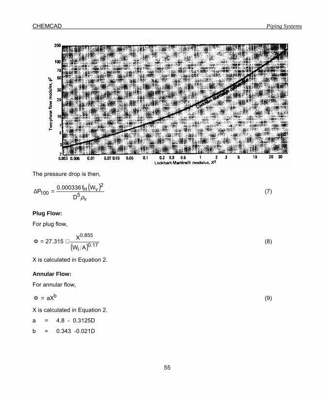
CHEMCAD Piping Systems
55
The pressure drop is then,
( )v
5
2vH
100D
Wf000336.0Pρ
=∆ (7)
Plug Flow:
For plug flow,
( ) 17.0l
855.0
AW
X315.27 ∗=Φ (8)
X is calculated in Equation 2.
Annular Flow:
For annular flow,
baX=Φ (9)
X is calculated in Equation 2.
a = 4.8 - 0.3125D
b = 0.343 -0.021D

Piping Systems CHEMCAD
56
Nomenclature:
A = Internal cross section of pipe, ft2
D = Internal diameter of pipe, ft.
L = Equivalent length of pipe and fittings, ft.
W = Flowrate, lb/h
∆P = Pressure loss, psi
µ = Viscosity, cp
ρ = Density, lb/ft3
ST = Surface tension, dyne/cm
Subscripts:
l = Refers to liquid
v = Refers to vapor
100 = Refers to 100 ft. of pipe
Accounting for elevation differences:
The elevation component of pressure drop is found using the Flanigan method. Within this method, the elevation component is calculated using the general equation below:
∑ ⋅=∆ e
LfLl Z
144HP ρ
where,
HLf is calculated according to the formula:
( ) 006.1sg
Lfv3264.01
1H+
=
where,
∆P = Pressure drop
ρL = Density of the liquid
Ze = Elevation changes
vsg = Velocity of the gas

CHEMCAD Piping Systems
57
THE BAKER METHOD PROCEDURE
1) Assumptions
a. Two phase flow is isothermal b. Turbulence exists in both phases c. Vapor and liquid move at the same speed d. ∆P is not greater than 10% of Pin.
2) Procedure:
a. Determine flow regime using Baker Chart b. Calculate ∆P2Φ = ∆Pv ⋅ Φ2
3) Two Phase Flow Regime:
TYPE DESCRIPTION Bubble (froth) Liquid with dispersed bubbles of gas Plug Alternating plugs of gas and liquid in the upper section of pipe. Stratified Liquid on the lower and gas on the upper section of the pipe separated
by a smooth interface. Wave Same as stratified, except separated by a wavy interface traveling in
the same direction of flow Slug Similar to stratified, except the gas periodically picks up a wave and
forms a bubbly plug. This flow can cause severe and dangerous vibrations because of the impact of the high-velocity slugs against the equipment.
Annular Gas in the center and liquid on the outer portion of the pipe. Spray (dispersed) Liquid droplets in the gas.
a. vl
VA
W16.2Byρρ
⋅=
where, wv = mass flowrate of the vapor A = pipe cross-sectional area ρi = density of liquid ρv = density of vapor

Piping Systems CHEMCAD
58
b.
=
STWW531B
31
32
l
l
vl
vl
xµ
ρ
ρρ
where, w1 = mass flowrate of liquid µ1 = liquid viscosity ST = liquid surface tension
c. Using By and Bx, read flow regime from Baker Chart.
4) Calculate ∆∆∆∆Pv,100:
vv
v DW31.6Re
µ=
fr is then read from Moody friction factor chart.
v5
2vv
100,vD
wf000336.0Pρ⋅
⋅⋅=∆
5) Calculate Lockhart-Martinelli Parameter,X2:
ll
l DW31.6Re
µ=
f is read from Moody friction factor chart.
2.0
vl
lv
8.1
vl2
ff
WWX
=
ρρ
2XX =
6) Calculate ΦΦΦΦ2:
a. Dispersed flow:
Φ2 read from Lockhart-Martinelli chart.
b. Bubble flow:
( ) 1.0
75.02.14AWX
l
=Φ
c. Slug flow:
( )AW
X1190
l
815.0=Φ

CHEMCAD Piping Systems
59
d. Stratified flow: (Horizontal Pipe)
( ) 8.0l AW
X15400=Φ
e. Plug flow: (Horizontal Pipe)
( ) 17.0l
855.0
AW
X315.27=Φ
f. Annular
bXa ⋅=Φ
a = 4.8 - 0.3125 D
b = 0.343 - 0.021 D
D = pipe ID, inches (for D > 12; use D = 10)
g. Wave flow:
=
vl
vl
x WWH
µµ
Read fh from the Huntington Chart
( )v
5
2vH
100,waveD
Wf000336.0Pρ
=∆
7) Calculate ∆∆∆∆P2ΦΦΦΦ,100:
2100,v100,2 PP Φ⋅∆=∆ Φ
THE BEGGS AND BRILL METHOD FOR TWO PHASE FLOW CALCULATIONS
The Beggs and Brill correlation was developed from experimental data obtained in a small-scale test facility. The facility consisted of 1-inch and 1.5-inch sections of acrylic pipe 90 feet long. The pipe could be inclined at any angle. The parameters studied and their range of variation were:
1) Gas flow rates of 0 to 300 Mscf/D;
2) Liquid flow rates of 0 to 30 gpm;
3) Average system pressure of 35 to 95 psia;
4) Pipe diameter of 1 and 1.5 inches;
Piping Systems CHEMCAD
60
5) Liquid hold-up of 0 to 0.87;
6) Pressure gradients of 0 to 0.8 psi/ft.; and
7) Inclination angles of �90 degrees to +90 degrees.
Fluids used were air and water. For each pipe size, liquid and gas rates were varied so that all flow patterns were observed. After a particular set of flow rates was set, the angle of the pipe was varied through the range of angles so that the effect of angle on holdup and pressure gradient could be observed. Liquid holdup and pressure gradient were measured at angles from horizontal of 0, plus and minus 5,10,15, 20, 35, 55, 75, and 90 degrees. The correlations were developed from 584 measured tests.
HORIZONTAL FLOW
Different correlations for liquid holdup are presented for each of the three horizontal flow regimes. The liquid holdup, which would exist if the pipe were horizontal, is first calculated and then corrected for the actual pipe inclination. Three of the horizontal flow patterns are illustrated in Figure 7-1. A fourth, the transition region, was added by Beggs and Brill to produce the map shown in Figure 7-2. The variation of liquid holdup with pipe inclination is shown in Figure 7-3 for three of the tests. The holdup was found to be a maximum at approximately +50 degrees from horizontal and a minimum at approximately �50 degrees. A two-phase friction factor is calculated using equations, which are independent of flow regime, but dependent on holdup. A graph of a normalized friction factor as a function of liquid holdup and input liquid content is given in Figure 7-4.

CHEMCAD Piping Systems
61
Figure 7-1 Horizontal Flow Patterns

Piping Systems CHEMCAD
62
Figure 7-2 Input L iquid ContentHorizontal F low Pattern M ap

CHEMCAD Piping Systems
63
Figure 7-3 Angle of Pipe from Horizontal Liquid Holdup vs Angle

Piping Systems CHEMCAD
64
Figure 7-4 Input Liquid Content Two-phase Friction Factor
FLOW REGIME DETERMINATION
The following variables are used to determine which flow regime would exist if the pipe were in a horizontal position. This flow regime is a correlating parameter and gives no information about the actual flow regime unless the pipe is completely horizontal.
gdV
Fr2m= (Froude No.)
m
SLL V
V=λ
0.302L1 316L λ=

CHEMCAD Piping Systems
65
-2.4684L2 0009252.0L λ=
-1.4516L3 10.0L λ=
-6.738L4 5.0L λ=
The horizontal flow regime limits are:
Segregated: λL < 0.01 and FR < L1
or
λL > 0.01 and FR < L2
Transition: λL > 0.01 and L2 < Fr < L3
Intermittent: 0.01 < λL < 0.4 and L3 < Fr < L1
or
λL > 0.4 and L3 < Fr < L4
Distributed: λL < 0.4 and Fr > L1
or
λL > 0.4 and Fr > L4
When the flow falls in the transition region, the liquid holdup must be calculated using both the segregated and the intermittent equations and interpolated using the following weighting factors:
HL(transition) = A x HL(segregated) + B x HL(intermittent)
where:
233
LLrFL
A−−
=
A-1B =
TWO-PHASE DENSITY
ρs = ρLHL + ρgHg
HL(φ) = ϕHL(0)
where,
HL(0) = the holdup which would exist at the same conditions in a horizontal pipe
HL(0) = (aλLb)/(Fr)c

Piping Systems CHEMCAD
66
For HL(0) > λL;
a b c
For segregated flow 0.98 0.4846 0.0868
For intermittent flow 0.845 0.5351 0.0173
For distributed flow 1.065 0.5824 0.0609
) be must(H L (o) L λ≥
The factor for correlating the holdup for the effect of pipe inclination is given by:
( ) ( )
−+=Ψ φφ 8.1sin333.08.1sinC1 3
where,
θ = the actual angle of the pipe from horizontal
C = (1 - λL) ln(D ∗ λLe ∗ NLV
f ∗ Frg)
d e f g
For segregated uphill 0.011 -3.768 3.539 -1.614
For intermittent uphill 2.96 0.305 -0.4473 0.0978
For distributed uphill No correction c = 0, Ψ = 1, HL ≠ f (ø)
For all downhill 4.7 -0.3692 0.1244 -0.5056
with the restriction that C > 0.
FRICTION FACTOR
Dg2Vf
ddP
c
2mntp
f •
••=
Ζ
ρ
where,
( )LgLggLLn 1 λρλρλρλρρ −•+•=•+•=
( )LgLLggL Ln 1mm λλµλλµµ −•+•=•+•=
nmn
RendVN
µρ ••=
ftp = fn ∗ X
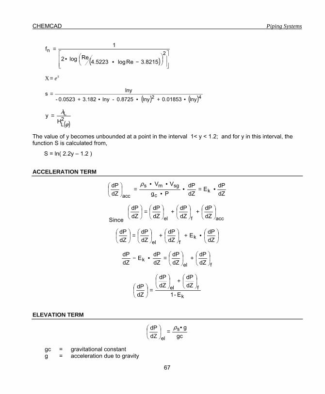
CHEMCAD Piping Systems
67
( )
−••
=2n
8215.3Re log 4.5223Relog2
1f
Se=X
( ) ( )42 lny01853.0lny 0.8725 -lny 3.1820.0523-
lnys•+••+
=
( )2L
LH
yφ
λ=
The value of y becomes unbounded at a point in the interval 1< y < 1.2; and for y in this interval, the function S is calculated from,
S = ln( 2.2y � 1.2 )
ACCELERATION TERM
dZdPE
dZdP
Pg
VV
dZdP
kc
sgms
acc•=•
•
••=
ρ
Since accfel dZdP
dZdP
dZdP
dZdP
+
+
=
•+
+
=
dZdPE
dZdP
dZdP
dZdP
kfel
felk dZ
dPdZdP
dZdPE
dZdP
+
=•−
k
felE-1
dZdP
dZdP
dZdP
+
=
ELEVATION TERM
gcg
ddP s
el
•=
Ζ
ρ
gc = gravitational constant g = acceleration due to gravity

Piping Systems CHEMCAD
68
VERTICAL FLOW
For vertical flow, θ = 1, and dL = dZ, so;
accfel dZdP
dZdP
dZdP
dZdP
dLdP
+
+
==
The pressure drop caused by elevation change depends on the density of the two-phase mixture and is usually calculated using a liquid holdup value. Except for high velocity situations, most of the pressure drop in vertical flow is caused by elevation change. The frictional pressure loss requires evaluation of the two-phase friction factor. The acceleration loss is usually ignored except for high velocity cases.
VERTICAL FLOW REGIMES
Bubble flow: In bubble flow the pipe is almost completely filled with liquid and the free gas phase is present in small bubbles. The bubbles move at different velocities and except for their density, have little effect on the pressure gradient. The wall of the pipe is always contacted by the liquid phase.
Slug flow: In slug flow the gas phase is more pronounced. Although the liquid phase is still continuous, the gas bubbles coalesce and form plugs or slugs, which almost fill the pipe cross section. The gas bubble velocity is greater than that of the liquid. The liquid in the film around the bubble may move downward at low velocities. Both the gas and liquid have significant effects on the pressure gradient.
Transition flow: The change from a continuous liquid phase to a continuous gas phase is called transition flow. The gas bubbles may join and liquid may be entrained in the bubbles. Although the liquid effects are significant, the gas phase effects are predominant.
Mist flow: In mist flow, the gas phase is continuous and the bulk of the liquid is entrained as droplets in the gas phase. The pipe wall is coated with a liquid film, but the gas phase predominantly controls the pressure gradient.
Illustrations of bubble, slug, transition, and mist flow are given in Figure 5-5 below.

CHEMCAD Piping Systems
69
F ig ure 7 -5 V ertica l F low P attern s A typical two-phase flow regime map is shown in Figure 7-6.
where,
NLv
Ngv Flow Regime Map
Figure 7-6

Piping Systems CHEMCAD
70
41
TSgVN L
SLLV
=
ρ
41
TSgVN L
SVGV
=
ρ
21
STg
dN LD
=
ρ
41
3L
LLST
gN
=
ρµ
LVN3650LS +=
0.75LVM N8475L +=
procedure for calculating vertical flow with the beggs and brill equation.
SET UP CALCULATIONS
1) Given:
a) Inlet ST,,,, ,m ,m LvLvLv µµρρ b) Pipe inside diameter, D c) Acceleration of gravity, g, 2s
ft
d) Inlet pressure, P
2) Calculate 4DA
2π=
3) Calculate Volumetric Flowrates: L
LLvvg
mQ&mQ ρρ ==
4) Calculate Superficial Velocities mslsg V,V,V
slsgmL
slg
sg VVVA
QV
AQ
V +===

CHEMCAD Piping Systems
71
I. DETERMINE FLOW REGIME
5) Calculate FROUDE gDv
RFNo.2m==
6) Calculate No-slip liquid holdup msl
L vv
== λ
7) Calculate dimension less �L� parameters:
302.0L1 316L λ=
4684.2L2 0009252.0L −= λ
4516.1L3 10.0L −= λ
738.6L4 5.0L −= λ
8) Apply flow regime rules:
a. Is ?LrFand01.0 1L ⟨⟨λ
↓→ flow SegregatedYesNo
b. Is ?LrFand01.0 2L ⟨≥λ
↓→
flow SegregatedYesNo
c. Is 32L LrFLand01.0 ≤≤≥λ ?
↓→ flow TransitionYesNo
d. Is 13L LrFLand4.001.0 ≤⟨⟨≤ λ ?
↓→ flow ntIntermitteYesNo
e. Is 43L LrFLand4.0 ≤⟨≥λ ?
↓→
flow ntIntermitteYesNo
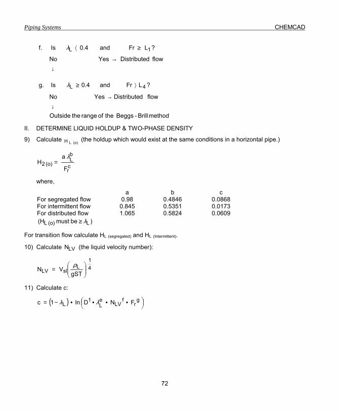
Piping Systems CHEMCAD
72
f. Is 1L LrFand4.0 ≥⟨λ ?
↓→
flow dDistributeYesNo
g. Is 4L LrFand4.0 ⟩≥λ ?
method Brill - Beggs the of range the Outside
flow dDistributeYesNo↓
→
II. DETERMINE LIQUID HOLDUP & TWO-PHASE DENSITY
9) Calculate (o) LH (the holdup which would exist at the same conditions in a horizontal pipe.)
cr
bL
(o) 2F
aH
λ=
where,
a b c For segregated flow 0.98 0.4846 0.0868 For intermittent flow 0.845 0.5351 0.0173 For distributed flow 1.065 0.5824 0.0609
) be must(H L (o) L λ≥
For transition flow calculate HL (segregated) and HL (Intermittent).
10) Calculate LVN (the liquid velocity number):
41
LslLV TSg
VN
=
ρ
11) Calculate c:
( )
••••−= g
rf
LVeL
1L FND ln1c λλ
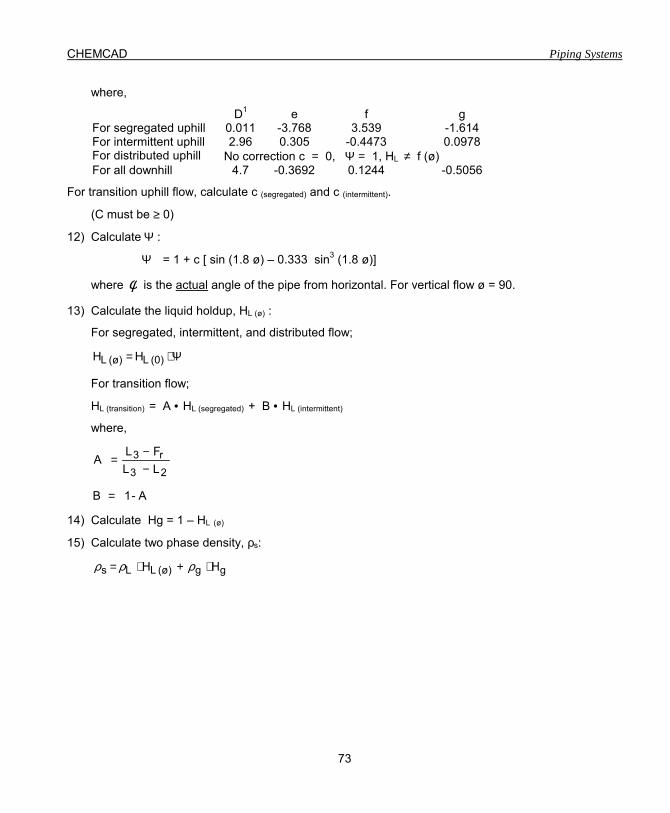
CHEMCAD Piping Systems
73
where,
D1 e f g For segregated uphill 0.011 -3.768 3.539 -1.614 For intermittent uphill 2.96 0.305 -0.4473 0.0978 For distributed uphill No correction c = 0, Ψ = 1, HL ≠ f (ø) For all downhill 4.7 -0.3692 0.1244 -0.5056
For transition uphill flow, calculate c (segregated) and c (intermittent).
(C must be ≥ 0)
12) Calculate Ψ :
Ψ = 1 + c [ sin (1.8 ø) � 0.333 sin3 (1.8 ø)]
where φ is the actual angle of the pipe from horizontal. For vertical flow ø = 90.
13) Calculate the liquid holdup, HL (ø) :
For segregated, intermittent, and distributed flow;
Ψ⋅= (0) L(ø) L H H
For transition flow;
HL (transition) = A • HL (segregated) + B • HL (intermittent)
where,
23r3
LLFL
A −−
=
A- 1B =
14) Calculate Hg = 1 � HL (ø)
15) Calculate two phase density, ρs:
gg(ø) LLs HH ⋅+⋅= ρρρ
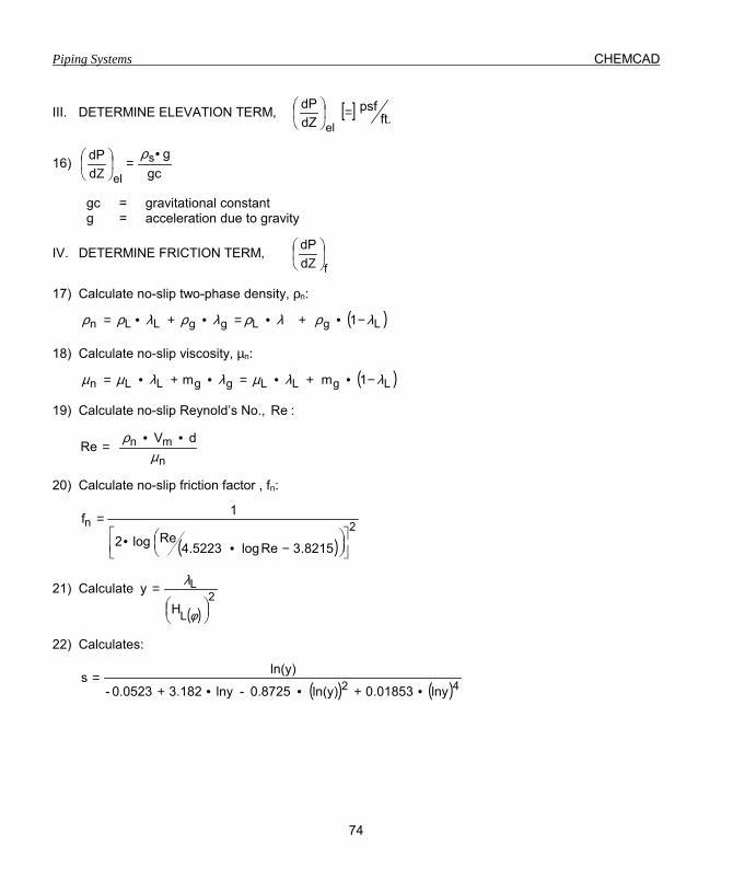
Piping Systems CHEMCAD
74
III. DETERMINE ELEVATION TERM, [ ] ft.psf
dZdP
el=
16) gc
gddP s
el
•=
Ζ
ρ
gc = gravitational constant g = acceleration due to gravity
IV. DETERMINE FRICTION TERM, fd
dP
Ζ
17) Calculate no-slip two-phase density, ρn:
( )LgLggLLn 1 λρλρλρλρρ −•+•=•+•=
18) Calculate no-slip viscosity, µn:
( )LgLLggL Ln 1mm λλµλλµµ −•+•=•+•=
19) Calculate no-slip Reynold�s No., Re :
nmn dV
Reµ
ρ ••=
20) Calculate no-slip friction factor , fn:
( )2n
8215.3Re log 4.5223Relog2
1f
−••
=
21) Calculate
( )2
L
L
Hy
=
φ
λ
22) Calculates:
( ) ( )42 lny01853.0ln(y) 0.8725 -lny 3.1820.0523-
ln(y)s•+••+
=
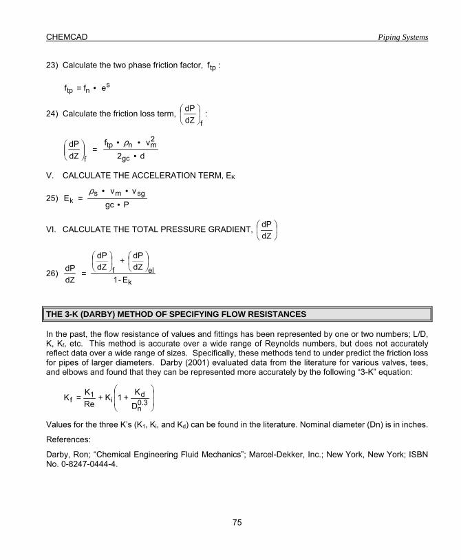
CHEMCAD Piping Systems
75
23) Calculate the two phase friction factor, tpf :
sntp eff •=
24) Calculate the friction loss term, fd
dP
Ζ
:
d2vf
ddP
gc
2mntp
f •
••=
Ζ
ρ
V. CALCULATE THE ACCELERATION TERM, EK
25) Pgc
vvE sgms
k •
••=
ρ
VI. CALCULATE THE TOTAL PRESSURE GRADIENT,
Ζd
dP
26) k
elfE - 1
ddP
ddP
ddP
Ζ+
Ζ=
Ζ
THE 3-K (DARBY) METHOD OF SPECIFYING FLOW RESISTANCES
In the past, the flow resistance of values and fittings has been represented by one or two numbers; L/D, K, Kf, etc. This method is accurate over a wide range of Reynolds numbers, but does not accurately reflect data over a wide range of sizes. Specifically, these methods tend to under predict the friction loss for pipes of larger diameters. Darby (2001) evaluated data from the literature for various valves, tees, and elbows and found that they can be represented more accurately by the following �3-K� equation:
++= 0.3
n
di
1f
D
K1KReKK
Values for the three K�s (K1, Ki, and Kd) can be found in the literature. Nominal diameter (Dn) is in inches.
References:
Darby, Ron; �Chemical Engineering Fluid Mechanics�; Marcel-Dekker, Inc.; New York, New York; ISBN No. 0-8247-0444-4.

Piping Systems CHEMCAD
76
HEAT LOSS IN PIPING SYSTEMS
The PIPE module will calculate the heat lost (or gained) to the surroundings if the user enters the overall heat transfer coefficient, U, and the ambient temperature, Ta. The heat loss is calculated like so;
( )ba TTAUQ −∗∗=
where, Q = the heat transferred to the surroundings (negative indicator heat lost from the piping system).
U = the overall heat transfer coefficient (user specified). Ta = the ambient temperature (user specified). Tb = the temperature of the bulk material in the pipe.
NET POSITIVE SUCTION HEAD
Centrifugal pumps require vapor free liquid flow in the suction line at the entrance to the impeller vanes to operate satisfactorily. Reciprocating pumps require such flow right after the inlet valve.
A centrifugal pump cannot pump vapor-liquid mixtures. A positive-displacement pump can pump liquids containing vapor but its volumetric efficiency will be greatly reduced � even if the weight percentage of vapor is a very small proportion of total flow.
The pressure gradient along the liquid path through a pump has characteristics similar to those of a control valve or orifice. Instead of a pressure loss, however, the downstream pressure will become much greater than the suction pressure, as sketched in Fig. 1. In both the pump-suction line and the pump, the minimum pressure should not drop below the vapor pressure of the liquid at the flowing temperature.
NET POSITIVE SUCTION HEAD
If the pressure in a centrifugal pump falls below the vapor pressure of the liquid at the flowing temperature, bubbles form just before the inlet edge of the impeller vanes. Because of the rapid increase in pressure within the impeller, the bubbles then collapse. This phenomenon is called cavitation. It can reduce pump efficiency and cause noise, vibration, impeller wear and breakage.
To avoid cavitation, pump manufacturers require a positive suction pressure called net positive suction head, NPSH. NPSH is the pressure above vapor pressure of the liquid being pumped, as measured as the pump-suction flange on a gage at the pump centerline. It is the pressure necessary to overcome friction and turbulence losses between the suction nozzle and the entrance to the impeller, and is usually given as head of water on pumps� head-capacity curves. NPSH, for a pump will increase with flowrate, and considerably increase with rotating speed of the impeller =
(NSPHr)2 = (n2/n1)2(NPSHr)1 (1)
where (NSPHr)2 is the required net positive suction head if pump speed is increased to n2 rpm. (NPSHr)1 and n1 are obtained from the pump�s head-capacity curve. For flows below about 20 to 25%
CHEMCAD Piping Systems
77
of rated capacity (near the maximum efficiency points), NPSH requirements can be higher than those for normal flow. This is especially true with high-capacity, low-head pumps.
Available net positive suction head, NPSHa, is the potential energy of an installation, expressed in feet of liquid head, and can be calculated from:
(NPSHa)(ρ)/144 = P (2)
where ρ = density of liquid at flowing temperature, lb/ft3; and P = pressure above vapor pressure at the centerline of the suction flange, psi.
If we let ρ = (SG)(ρw), where ρω = density of water at 60o F, 62.37 lb/ft3, and SG = specific gravity of liquid at flowing temperature, Eq. (2) becomes:
NPSHa = 2.31 P/SG (3)
To ensure reliable pump operation, NPSHa should equal or exceed NPSHr. Thus, process equipment must be elevated at least as high as the sum of the pump�s NPSHr, plus the friction-head losses in the suction line when saturated liquids are pumped.
At the suction nozzle, velocity head is also a positive energy component. However, this is not included in NPSH diagrams for pumps made in the U.S. Consequently, in calculations for NPSHa, velocity head does not have to be considered.
According to the Hydraulic Institute �The NPSH requirements of centrifugal pumps are normally determined on the basis of handling water. It is recognized that when pumping hydrocarbons, the NPSH to obtain satisfactory operation may be reduced for certain conditions.� However, it is customary to use manufacturers� data for the minimum required NPSH when handling hydrocarbons having specific gravities less than 1. This means that (1) both available and required NPSH do not vary with the liquid�s specific gravity, (2) for a given centrifugal pump, one curve of required NPSH can be used with all normal specific gravities.
The effect of specific gravity can be explained as follows: Looking at the analogy of NPSH as a force that pushes liquid into a pump, and assuming a pump that has an NPSHr of 8 ft. at a given capacity, we can show that a head of 8 ft. of water equals 3.45 psi, while a head of 8 ft. of gasoline equals 2.60 psi. It would appear that the force pushing liquid into the pump decreases with specific gravity. However, the mass of liquid being accelerated has decreased by the same proportion.
When choosing between two pumps of equal capacity, the one having the higher NPSHr will cost less. But the less-expensive pump will be the economic choice only if its cost advantage is not offset by the expense of elevating the process equipment. Often, a vertical pump will be specified to bring equipment closer to grade elevation.
If a reciprocating pump is to transfer saturated liquid and if we desire maximum volumetric efficiency, we make analyses and calculations for NPSH conditions similar to those for centrifugal pumps. Resistance at the inlet valve of a reciprocating pump is greater than the entrance loss to an impeller. Sue to pulsating liquid flow, we must also take into account increased line resistance.

Piping Systems CHEMCAD
78
PUMPING SATURATED LIQUIDS
For subcooled liquids, the available pressure at the suction nozzle is usually more than adequate for NPSH and line losses. Consequently, suction vessels can be close to grade elevation, and the pipe configuration is not as critical.
Many process pumps handle saturated liquids. Here, the suction vessel and drawoff nozzle are elevated to meet the NPSH requirement, plus a distance equal to the static height of the line losses.
We now repeat an important rule for the design engineer. At no point in the suction line should pressure fall (due to piping and components resistance) below the vapor pressure of the liquid at the flowing temperature. A horizontal pipe run immediately after the drawoff nozzle is undesirable because a gradual pressure reduction (in proportion to the length of horizontal pipe) can cause the liquid to vaporize. Also, if the liquid level in the suction vessel is low, the available static head might not be sufficient to compensate for the exit loss and the friction loss in the horizontal pipe section. This is especially true with light, volatile liquids.
A horizontal-pipe segment after a vertical drop is not as bad because static head is available at the beginning of the horizontal section. In a vertical segment of suction piping, the potential energy is usually much greater than the energy consumed by friction. Thus, when pumping hot liquids, a vertical pipe run after the drawoff nozzle is most desirable; and with light hydrocarbons, it can become essential.
To avoid vaporization at the vessel�s drawoff nozzle, the minimum static head of liquid above the nozzle should be greater than the entrance loss to the suction pipe. Cavitation at the drawoff nozzle can cause undesirable pressure surges and inconsistent control conditions.
The exit resistance of a nozzle can be expressed:
g2vKh
2L ⋅= (4
where hL is liquid level above drawoff nozzle, ft; K = 0.5, the resistance coefficient for a sharp-edged pipe entrance; v is flow velocity, ft/s; and g is gravitational constant, 32.2 ft/s2.
Using a safety factor of four, the minimum liquid head above the drawoff nozzle will be:
hL = 4K
PIPE SIZING USING THE KENT METHOD
If you close the general pipe sizing method of CHEMCAD, the diameter is determined based upon �typical� velocities which are a function of fluid density. These typical velocities result in the following equations for diameter:
For liquids:
434.0W607.2D
=
ρ

CHEMCAD Piping Systems
79
For gases:
343.0
408.0W065.1Dρ
=
where, D = Pipe internal dia., in. W = Flowrate, 1000lb/h ρ = Density, lb/ft3
Reference:
�Preliminary Pipeline Sizing� ; George R. Kent; Chemical Engineering; September 25, 1978.

Piping Systems CHEMCAD
80
VARIABLE DEFINITIONS
A = Flow area D = Diameter Ek = Beggs and Brill acceleration term Fr = Froude number f = Friction factor gc = Gravitational constant H = Holdup h = enthalpy L = Length M = Molecular weight NPSHa = Available net positive suction head P = pressure PLW = Losses due to irreversible processes q = Heat loss (input) Q = Volumetric flowrate Re = Reynold�s number S = Entropy SG = Specific gravity ST = Surface tension U = Internal energy V = Volume v = Velocity W = Mass flowrate X = Dimensionless flow pattern region coefficient Y = Flow pattern region coefficient Z = Elevation λ = Slip µ = Viscosity Φ = Lockhart�Martenelli correlating parameter ρ = Density τ = Shear force 2Φ = Two phase

CHEMCAD Piping Systems
81
CHAPTER 8 – DESCRIPTIONS OF VALVES AND FITTINGS
Valves
1. Gate valve 2. Globe seat flat, bevel, plug 3. Globe wing/pin guided disk 4. Angle, no obstruction 5. Angle wing/pin guided disc 6. Y-pattern globe 60 deg 7. Y-pattern globe 45 deg 8. Ball valve 9. Butterfly 2-8 inches 10. Butterfly 10-14 inches 11. Butterfly 14-24 inches 12. Plug, straight-way 13. Plug, 3-way (straight way) 14. Plug, 3-way through branch 15. Foot valve, poppet disk 16. Foot valve, hinged disk 17. Swing check, clearway 18. Swing check, tilting seat 19. Tilt disk 5 deg 2-8 in 20. Tilt disk 5 deg 10-14 in 21. Tilt disk 5 deg 16-48 in 22. Tilt disk 15 deg 2-8 in 23. Tilt disk 15 deg 10-14 in 24. Tilt disk 15 deg 16-48 in 25. Lift of stop check, globe 26. Lift or stop check, angle
Flanged Fittings
27. Standard elbow 90 deg 28. Standard elbow 45 deg 29. Standard elbow 90 long R 30. Return bend 180 deg close 31. Standard T, flow-through run 32. Standard T, flow-through branch 33. 45 deg T, flow-through run 34. 45 deg T, flow-through barnch 35. Elbow 90 deg, R/D = 1.0 36. Elbow 90 deg, R/D = 1.5 37. Elbow 90 deg, R/D = 2.0

Piping Systems CHEMCAD
82
Welded Fittings
38. Elbow 45 deg, R/D = 1.0 39. Elbow 45 deg, R/D = 1.5 40. Elbow 45 deg, R/D = 2.0 41. Return bend 180, R/D = 1.0 42. Return bend 180, R/D = 1.5 43. Return bend 180, R/D = 2.0 44. Tee 100% flow-through run 45. Tee 100% flow-out branch 46. Tee 100% flow-in branch 47. Reducer
Miscellaneous
48. Entrance, inward project 49. Entrance, sharp edged 50. Entrance, slightly round 51. Entrance, well rounded 52. Exit from pipe 53. Sudden contraction 54. Sudden expansion, For sudden contraction/expansion: small dia./large dia.
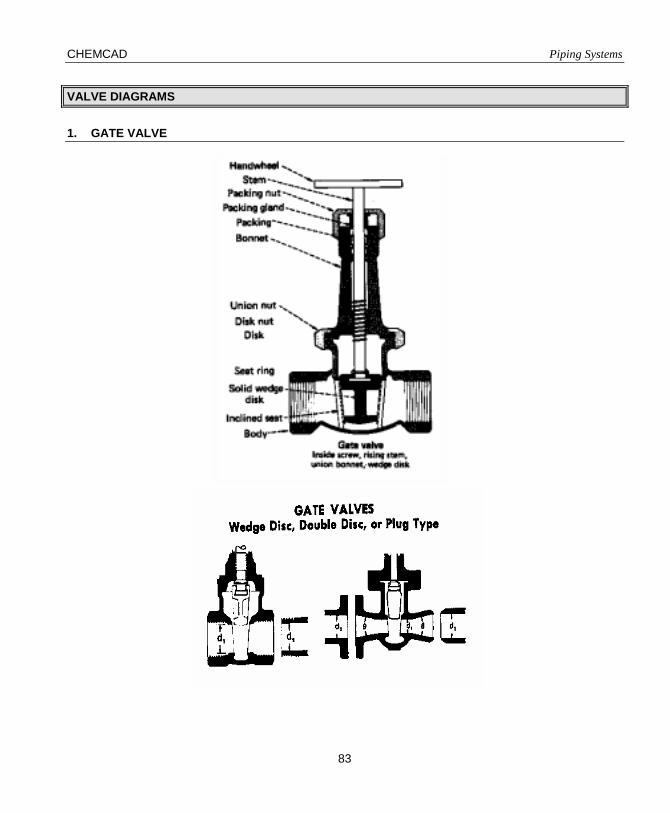
CHEMCAD Piping Systems
83
VALVE DIAGRAMS
1. GATE VALVE
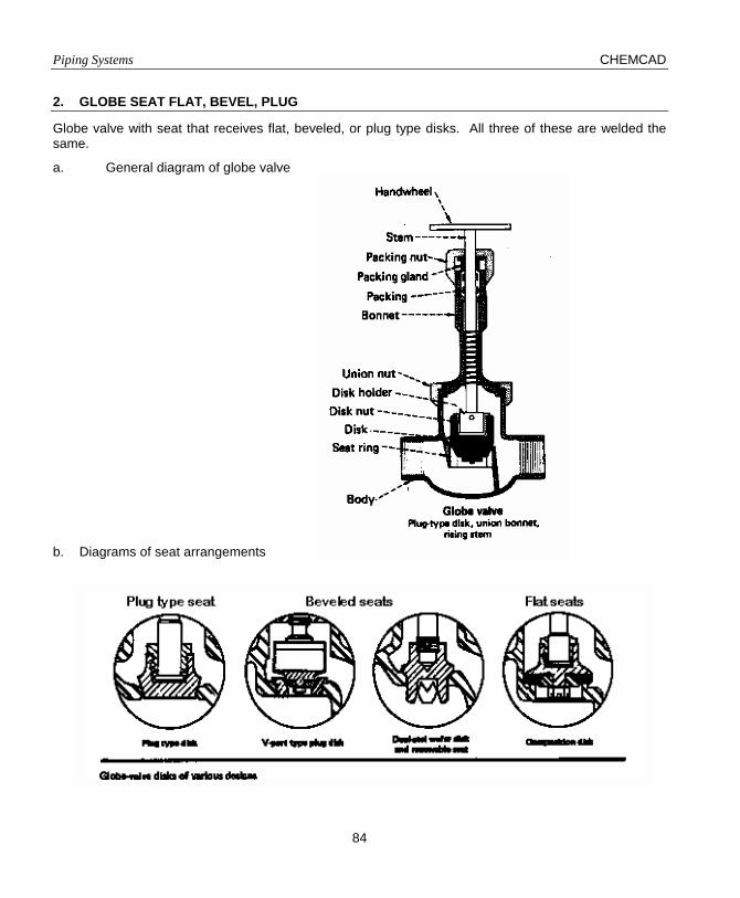
Piping Systems CHEMCAD
84
2. GLOBE SEAT FLAT, BEVEL, PLUG
Globe valve with seat that receives flat, beveled, or plug type disks. All three of these are welded the same.
a. General diagram of globe valve
b. Diagrams of seat arrangements

CHEMCAD Piping Systems
85
3. GLOBE WING/PIN GUIDED DISK
Globe valve with disk guided by pin or wing.
Pin guided disk
4. ANGLE, NO OBSTRUCTION
Angle valve with no obstruction; that is, no disk guides.
Angle valves are basically globe valves having inlet and outlet connections at right angles.
The overall construction elements of an angle valve are basically the same for the stern, disk and seat-rings design as the globe valve.
DiskPin guide
General diagram of angle valves

Piping Systems CHEMCAD
86
5. ANGLE, WING/PIN GUIDED DISK
Angle valve with wing or pin disk guides.
6. Y-PATTERN GLOBE 60 DEGREES
Y-pattern globe valve with a 60 degree angle.
7. Y-PATTERN GLOBE 45 DEGREES
Y-pattern glove valve with a 45 degree angle.
General diagram
Y-pattern globe valve

CHEMCAD Piping Systems
87
8. BALL VALVE
General Diagram
T h i s a n gThis angle can be 45° or 60°
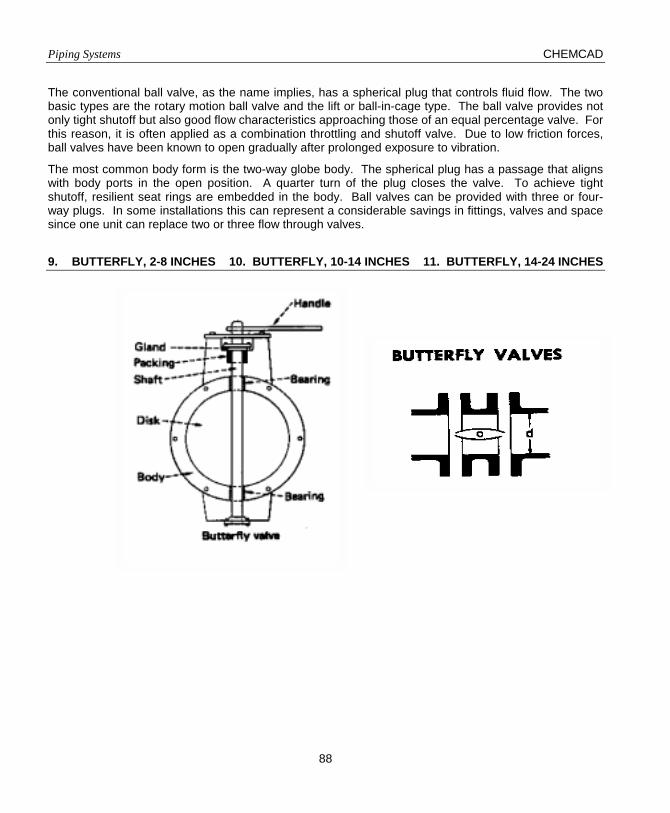
Piping Systems CHEMCAD
88
The conventional ball valve, as the name implies, has a spherical plug that controls fluid flow. The two basic types are the rotary motion ball valve and the lift or ball-in-cage type. The ball valve provides not only tight shutoff but also good flow characteristics approaching those of an equal percentage valve. For this reason, it is often applied as a combination throttling and shutoff valve. Due to low friction forces, ball valves have been known to open gradually after prolonged exposure to vibration.
The most common body form is the two-way globe body. The spherical plug has a passage that aligns with body ports in the open position. A quarter turn of the plug closes the valve. To achieve tight shutoff, resilient seat rings are embedded in the body. Ball valves can be provided with three or four-way plugs. In some installations this can represent a considerable savings in fittings, valves and space since one unit can replace two or three flow through valves.
9. BUTTERFLY, 2-8 INCHES 10. BUTTERFLY, 10-14 INCHES 11. BUTTERFLY, 14-24 INCHES

CHEMCAD Piping Systems
89
12. PLUG, STRAIGHT WAY
13. PLUG, 3-WAY (STRAIGHT RUN) 14. PLUG, 3-WAY THROUGH BRANCH
General diagram
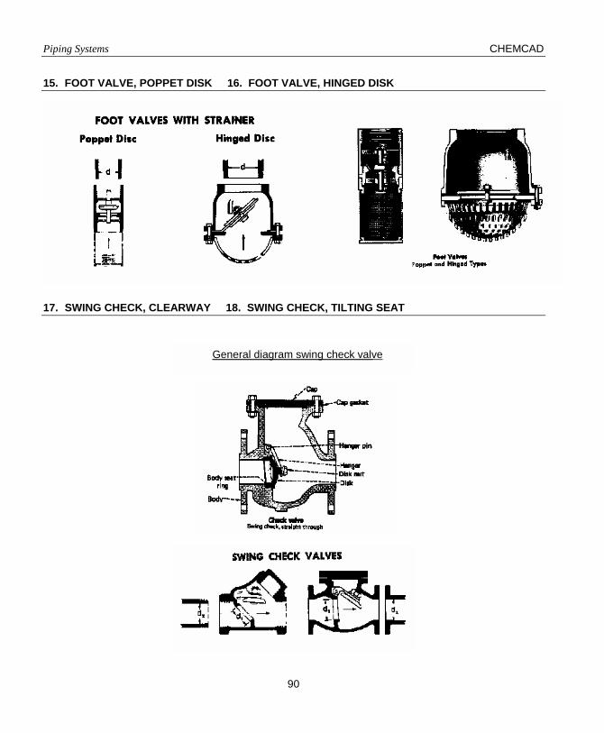
Piping Systems CHEMCAD
90
15. FOOT VALVE, POPPET DISK 16. FOOT VALVE, HINGED DISK
17. SWING CHECK, CLEARWAY 18. SWING CHECK, TILTING SEAT
General diagram swing check valve

CHEMCAD Piping Systems
91
19. TILT DISK, 5 DEGREES 2-8 IN 20. TILT DISK, 5-DEGREES 10-14 IN
21. TILT DISK, 5 DEGREES 16-48 IN 22. TILT DISK, 15 DEGREES 2-8 IN
23. TILT DISK, 15 DEGREES 10-14 IN 24. TILT DISK, 15 DEGREES 16-48 IN
25. LIFT OR STOP CHECK VALVE, GLOBE
Stop check valves, globe type
Lift check valves, globe type

Piping Systems CHEMCAD
92
Stop-check valves are usually produced in globe or angle styles, with a stem that is used either to tightly seat or to restrict the lift of the disk. The stem is not attached to the disk, and cannot be used to open the valve. The stop-check valve is used on steam lines from boilers more than in any other application.
Foot valves are specialty check valves used at the bottom of a suction line on a horizontal pump. They maintain the prime on such pumps and usually incorporate strainers to keep foreign matter from entering.
Lift check valves, usually of the globe body form, depend on gravity for operation. They are designed for either horizontal or vertical installation, but the two designs are not interchangeable. Under forward flow, a piston is lifted off the seat by fluid while being retained in the valve by guides. On reverse flow, the piston is forced against the seat to block further flow. Some lift check valves utilize spring loading to assure positive seating. In any case, lift check valves require relatively high pressure drops. They are used on higher pressure services and in smaller pipe sizes than swing checks.
26. LIFT OR STOP CHECK VALVES, ANGLE

CHEMCAD Piping Systems
93
FLANGED FITTINGS
27. STANDARD ELBOW, 90 DEGREES 28. STANDARD ELBOW, 45 DEGREES
29. STANDARD ELBOW, 90 LONG R
Standard elbows and fittings are built to standard dimensions which are given in mechanical standards like ANSI B16.5, ANSI B16.1, etc. The dimensions change with pressure rating.

Piping Systems CHEMCAD
94
30. RETURN BEND, 180 DEGREES, CLOSE (FLANGED)
A close return bend means that R/D = 1.
31. STANDARD T, FLOW-THROUGH RUN (FLANGED)
32. STANDARD T, FLOW-THROUGH BRANCH (FLANGED)
flow through branch
flow through run
FLANGED TEE

CHEMCAD Piping Systems
95
Standard T’s are built according to dimensions given in mechanical standards like DIN, ASNI B16.1, ANSI B16.5, etc. The dimensions change with pressure rating.
33. 45 DEG. T, FLOW THROUGH RUN (FLANGED)
34. 45 DEG. T, FLOW THROUGH BRANCH (FLANGED)
45o
flanged
flow through run flow through branch
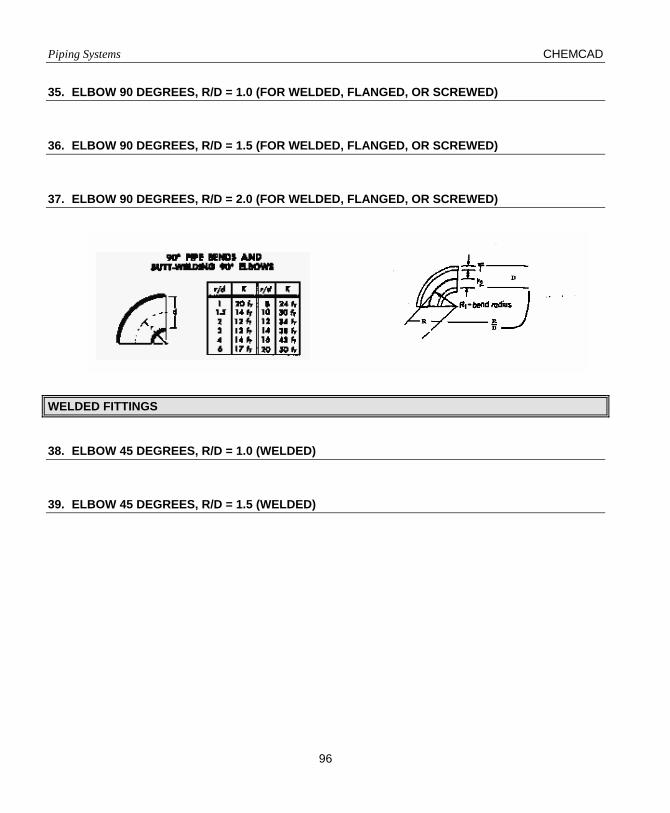
Piping Systems CHEMCAD
96
35. ELBOW 90 DEGREES, R/D = 1.0 (FOR WELDED, FLANGED, OR SCREWED)
36. ELBOW 90 DEGREES, R/D = 1.5 (FOR WELDED, FLANGED, OR SCREWED)
37. ELBOW 90 DEGREES, R/D = 2.0 (FOR WELDED, FLANGED, OR SCREWED)
WELDED FITTINGS
38. ELBOW 45 DEGREES, R/D = 1.0 (WELDED)
39. ELBOW 45 DEGREES, R/D = 1.5 (WELDED)

CHEMCAD Piping Systems
97
40. ELBOW 45 DEGREES, R/D = 2.0 (WELDED)
41. RETURN BEND 180, R/D = 1.0 (WELDED)
42. RETURN BEND 180, R/D = 1.5 (WELDED)
43. RETURN BEND 180, R/D = 2.0 (WELDED)
44. TEE 100% FLOW THROUGH RUN (WELDED)
45. TEE 100% FLOW OUT BRANCH (WELDED)
R/D as defined above
R/D same as for 90° elbow

Piping Systems CHEMCAD
98
46. TEE 100% FLOW IN BRANCH (WELDED)
47. REDUCER (WELDED)
Flow
flow through run flow though branch
Flow
Flow
flow in branch

CHEMCAD Piping Systems
99
MISCELLANEOUS
48. ENTRANCE, INWARD PROJECTING
49. ENTRANCE, SHARP EDGED
50. ENTRANCE, SLIGHTLY ROUNDED
51. ENTRANCE, WELL ROUNDED
Sharp edged inlet (24)

Piping Systems CHEMCAD
100
52. EXIT FROM PIPE
No distinction between types made in CHEMCAD.