CHEE320 - Fall 2001J. McLellan1 Joint Probability - Considering Several Random Variables Together...
87
CHEE320 - Fall 2001 J. McLellan 1 Joint Probability - Considering Several Random Variables Together and Regression Analysis CHEE320 Module 5
-
Upload
noreen-gray -
Category
Documents
-
view
217 -
download
1
Transcript of CHEE320 - Fall 2001J. McLellan1 Joint Probability - Considering Several Random Variables Together...

CHEE320 - Fall 2001
J. McLellan 1
Joint Probability - Considering Several Random Variables Together
andRegression Analysis
CHEE320
Module 5

CHEE320 - Fall 2001
J. McLellan 2
Outline
• considering outcomes of random variables together• discrete case - joint probability functions • continuous case - joint density functions• expected values - mean, variance, covariance• covariance - measure of systematic linear
relationships

CHEE320 - Fall 2001
J. McLellan 3
Considering Random Variables Jointly
In some instances, we may be interested in how several random quantities occur together - “jointly”
Examples:
Discrete - » automobile colours - {red, blue, green, black, silver}» automobile finish - {metallic, matte}» jointly - {(red,matte), (red,metallic), (blue,matte), (blue,
metallic), …}
Continuous - » composition -- 0.1< composition<0.5 g/L» temperature -- 300 C < temperature < 350 C » jointly -- (0.1 < composition<0.5, 300<T<350)

CHEE320 - Fall 2001
J. McLellan 4
Considering Random Variables Jointly
Graphical summary - bivariate histogram
Bivariate Histogram (EMISSION.STA 4v*21c) Frequency asa function of range ineach variable

CHEE320 - Fall 2001
J. McLellan 5
Joint Probabilities
In the joint situation, we consider events defined in terms of pairs of outcomes - one from each random variable.
We can summarize the probability of pairs of occurrences using probability function or probability density functions.
Note that in this instance, the functions are defined on the plane -- i.e., assigns probabilities to a pair of coordinates

CHEE320 - Fall 2001
J. McLellan 6
Joint Probabilities
Discrete Case - Joint probability function
e.g., car colour and finish:
),(),( yYxXPyxpXY
metallicybluexfor
matteybluexformetallicyredxfor
matteyredxfor
yxpXY
,2.0
,4.0,3.0
,1.0
),(
redblue
metallicmatte
pXY

CHEE320 - Fall 2001
J. McLellan 7
Joint Probabilities
Continuous Case - joint probability density function
and cumulative joint distribution function:
Example - bivariate Normal distribution function
),( yxfXY
1 2),(),(),( 2121
dxdyyxfYXPF XYXY
2
2
1
),(
),(
)21
exp()det(2
1),(
Y
X
y
xyxXY
YXCov
YXCovwhere
y
xyxyxf

CHEE320 - Fall 2001
J. McLellan 8
Joint Probabilities
Example - bivariate Normal distribution
CHEE320 - Fall 2001
J. McLellan 9
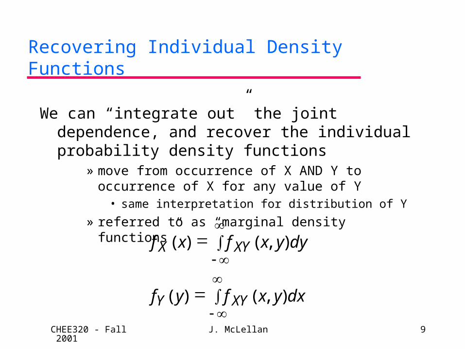
Recovering Individual Density Functions
We can “integrate out” the joint dependence, and recover the individual probability density functions
» move from occurrence of X AND Y to occurrence of X for any value of Y
• same interpretation for distribution of Y
» referred to as “marginal density functions”
dxyxfyf
dyyxfxf
XYY
XYX
),()(
),()(

CHEE320 - Fall 2001
J. McLellan 10
Expected Values
Given a function g(X,Y), we can define the expected value as:
Examples:» g(X,Y) = X - recover mean of X» mean of Y» covariance of X and Y -- to be discussed in regression
section
dxdyyxfyxgYXgE XY ),(),()},({

CHEE320 - Fall 2001
J. McLellan 11
Independence and Joint Distributions
Recall that independence implies that:
» similarly for continuous random variables, and cumulative distributions
This implies that
This plays a role for mean and variance of sample average.
)()()( yYPxXPyYxXP YX
)()(),( yfxfyxf YXXY

CHEE320 - Fall 2001
J. McLellan 12
Regression Analysis

CHEE320 - Fall 2001
J. McLellan 13
Outline
• assessing systematic relationships• types of models• least squares estimation - assumptions• fitting a straight line to data
» least squares parameter estimates» graphical diagnostics» quantitative diagnostics
• multiple linear regression » least squares parameter estimates» diagnostics
• precision of parameter estimates, predicted responses
CHEE320 - Fall 2001
J. McLellan 14
The Scenario
We have been given a data set consisting of measurements of a number of variables
PLUS» background information about the “process”» objectives for the investigation » information about how the experimentation was
conducted – e.g., shift, operating region, product line, ...

CHEE320 - Fall 2001
J. McLellan 15
Assessing Systematic Relationships
Is there a systematic relationship?Two approaches:
• graphical
• quantitative
Other points -
• what is the nature of the relationship?» linear in the “independent variables”
» nonlinear in the “independent variables”
• from engineering/scientific judgement - should there be a relationship?
CHEE320 - Fall 2001
J. McLellan 16
Assessing Systematic Relationships
Graphical Methods• scatterplots (x-y diagrams)
» plot values of one variable against another» look for evidence of a trend» look for nature of trend - linear, quadratic, exponential, other
nonlinearity?
• surface plots » plot one variable against values of two other variables» look for evidence of a trend - surface» look for nature of trend - linear, nonlinear?
• casement plots» a “matrix”, or table, of scatterplots

CHEE320 - Fall 2001
J. McLellan 17
Graphical Methods for Analyzing Data
Visualizing relationships between variables
Techniques
• scatterplots• scatterplot matrices
» also referred to as “casement plots”

CHEE320 - Fall 2001
J. McLellan 18
Scatterplots
,,, are also referred to as “x-y diagrams”• plot values of one variable against another • look for systematic trend in data
» nature of trend• linear?
• exponential?
• quadratic?
» degree of scatter - does spread increase/decrease over range?
• indication that variance isn’t constant over range of data

CHEE320 - Fall 2001
J. McLellan 19
Scatterplots - Example
Scatterplot (teeth 4v*20c)
FLUORIDE
DIS
CO
LO
R
5
10
15
20
25
30
35
40
45
50
0.0 0.5 1.0 1.5 2.0 2.5 3.0 3.5 4.0 4.5
trend - possiblynonlinear?
• tooth discoloration data - discoloration vs. fluoride

CHEE320 - Fall 2001
J. McLellan 20
Scatterplot - Example
Scatterplot (teeth 4v*20c)
BRUSHING
DIS
CO
LO
R
5
10
15
20
25
30
35
40
45
50
4 5 6 7 8 9 10 11 12 13
• tooth discoloration data -discoloration vs. brushing
signficant trend?- doesn’t appear tobe present

CHEE320 - Fall 2001
J. McLellan 21
Scatterplot - Example
Scatterplot (teeth 4v*20c)
BRUSHING
DIS
CO
LO
R
5
10
15
20
25
30
35
40
45
50
4 5 6 7 8 9 10 11 12 13
Variance appearsto decrease as # of brushings increases
• tooth discoloration data -discoloration vs. brushing
CHEE320 - Fall 2001
J. McLellan 22
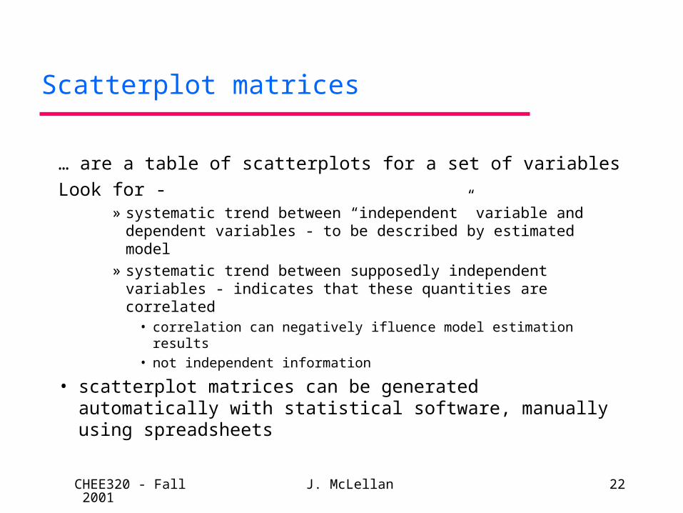
Scatterplot matrices
… are a table of scatterplots for a set of variables
Look for - » systematic trend between “independent” variable and
dependent variables - to be described by estimated model
» systematic trend between supposedly independent variables - indicates that these quantities are correlated
• correlation can negatively ifluence model estimation results
• not independent information
• scatterplot matrices can be generated automatically with statistical software, manually using spreadsheets

CHEE320 - Fall 2001
J. McLellan 23
Scatterplot Matrices - tooth data
Matrix Plot (teeth 4v*20c)
FLUORIDE
AGE
BRUSHING
DISCOLOR

CHEE320 - Fall 2001
J. McLellan 24
Assessing Systematic Relationships
Quantitative Methods
• correlation » formal def’n plus sample statistic (“Pearson’s r”)
• covariance» formal def’n plus sample statistic
provide a quantiative measure of systematic LINEAR relationships

CHEE320 - Fall 2001
J. McLellan 25
Covariance
Formal Definition
• given two random variables X and Y, the covariance is
• E{ } - expected value• sign of the covariance indicates the sign of the slope of the
systematic linear relationship» positive value --> positive slope
» negative value --> negative slope
• issue - covariance is SCALE DEPENDENT
Cov X Y E X YX Y( , ) {( )( )}

CHEE320 - Fall 2001
J. McLellan 26
Covariance
• motivation for covariance as a measure of systematic linear relationship
» look at pairs of departures about the mean of X, Y
X
Y
mean of X, Y
X
Y
mean of X, Y

CHEE320 - Fall 2001
J. McLellan 27
Correlation
• is the “dimensionless” covariance» divide covariance by standard dev’ns of X, Y
• formal definition
• properties» dimensionless » range
Corr X Y X YCov X Y
X Y( , ) ( , )
( , )
1 1( , )X Ystrong linear relationshipwith negative slope
strong linear relationshipwith positive slope
Note - the correlation gives NO information about the actual numerical value of the slope.

CHEE320 - Fall 2001
J. McLellan 28
Estimating Covariance, Correlation
… from process data (with N pairs of observations)
Sample Covariance
Sample Correlation
RN
X X Y Yi ii
N
11 1
( )( )
rN
X X Y Y
s s
i ii
N
X Y
1
1 1( )( )

CHEE320 - Fall 2001
J. McLellan 29
Making Inferences
The sample covariance and correlation are STATISTICS, and have their own probability distributions.
Confidence interval for sample correlation - » the following is approximately distributed as the standard
normal random variable
» derive confidence limits for and convert to confidence limits for the true correlation using tanhtanh ( )1
N r 3 1 1(tanh ( ) tanh ( ))

CHEE320 - Fall 2001
J. McLellan 30
Confidence Interval for Correlation
Procedure
1. find for desired confidence level
2. confidence interval for is
3. convert to limits to confidence limits for correlation by taking tanh of the limits in step 2
A hypothesis test can also be performed using this function of the
correlation and comparing to the standard normal distribution
z/2tanh ( )1
tanh ( ) /
1
21
3r
Nz

CHEE320 - Fall 2001
J. McLellan 31
Example - Solder Thickness
Objective - study the effect of temperature on solder thickness
Data - in pairsSolder Temperature (C) Solder Thickness (microns)
245 171.6
215 201.1
218 213.2
265 153.3
251 178.9
213 226.6
234 190.3
257 171
244 197.5
225 209.8

CHEE320 - Fall 2001
J. McLellan 32
Example - Solder Thickness
Solder Thickness (microns)
140150160170180190200210220230
200 210 220 230 240 250 260 270
temperature
thic
knes
s
Solder Temperature (C)Solder Thickness (microns)Solder Temperature (C) 1Solder Thickness (microns) -0.920001236 1

CHEE320 - Fall 2001
J. McLellan 33
Example - Solder Thickness
Confidence Interval
zalpha/2 of 1.96 (95% confidence level)
limits in tanh^-1(rho) -2.329837282 -0.848216548
limits in rho -0.981238575 -0.690136605

CHEE320 - Fall 2001
J. McLellan 34
Outline
• assessing systematic relationships
• types of models• least squares estimation - assumptions• fitting a straight line to data
» least squares parameter estimates» graphical diagnostics» quantitative diagnostics
• multiple linear regression » least squares parameter estimates» diagnostics
• precision of parameter estimates, predicted responses

CHEE320 - Fall 2001
J. McLellan 35
Empirical Modeling - Terminology
• response» “dependent” variable - responds to changes in other
variables» the response is the characteristic of interest which we are
trying to predict
• explanatory variable» “independent” variable, regressor variable, input, factor» these are the quantities that we believe have an influence
on the response
• parameter» coefficients in the model that describe how the regressors
influence the response
CHEE320 - Fall 2001
J. McLellan 36
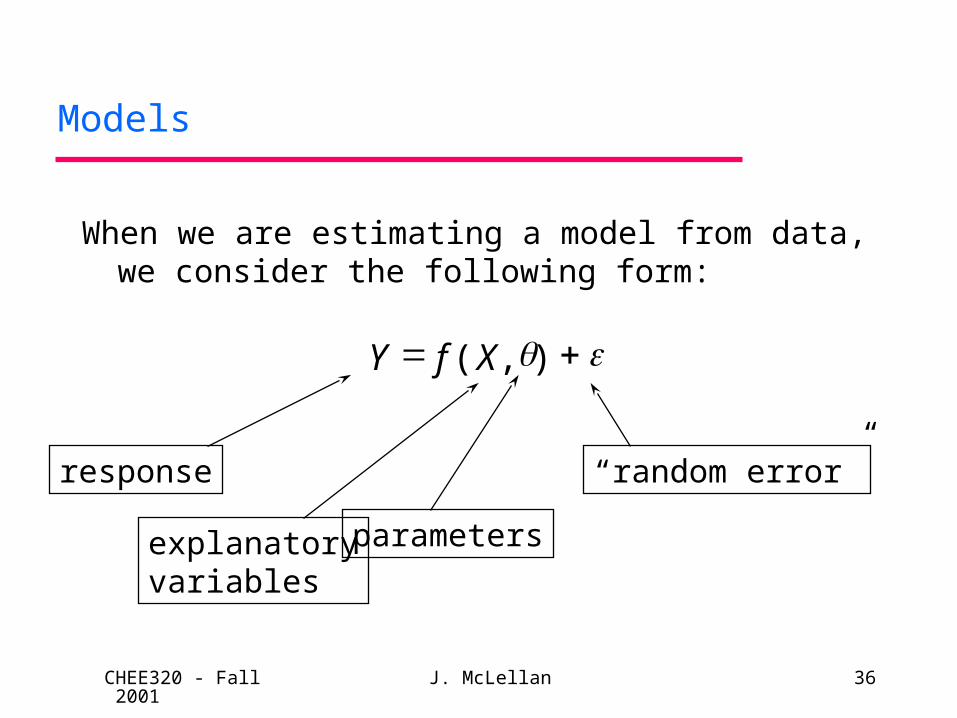
Models
When we are estimating a model from data, we consider the following form:
Y f X ( , )
response
explanatoryvariables
parameters
“random error”

CHEE320 - Fall 2001
J. McLellan 37
The Random Error Term
• is included to reflect fact that measured data contain variability
» successive measurements under the same conditions (values of the explanatory variables) are likely to be slightly different
» this is the stochastic component» the functional form describes the deterministic
component» random error is not necessarily the result of mistakes in
experimental procedures - reflects inherent variability» “noise”

CHEE320 - Fall 2001
J. McLellan 38
Types of Models
• linear/nonlinear in the parameters• linear/nonlinear in the explanatory variables• number of response variables
– single response (standard regression)– multi-response (or “multivariate” models)
From the perspective of statistical model-building,the key point is whether the model is linear or nonlinear in the PARAMETERS.

CHEE320 - Fall 2001
J. McLellan 39
Linear Regression Models
• linear in the parameters
• can be nonlinear in the regressors
T T T95 1 2 b bLGO mid
T T T95 1 2 b bLGO mid

CHEE320 - Fall 2001
J. McLellan 40
Nonlinear Regression Models
• nonlinear in the parameters– e.g., Arrhenius rate expression
r exp(RT
) k
E0
linear(if E is fixed)
nonlinear

CHEE320 - Fall 2001
J. McLellan 41
Nonlinear Regression Models
• sometimes transformably linear• start with
and take ln of both sides to produce
which is of the form
r exp(RT
) kE
0
ln(r) ln( )RT
kE
0
Y 0 11
RTlinear in theparameters

CHEE320 - Fall 2001
J. McLellan 42
Transformations
• note that linearizing the nonlinear equation by transformation can lead to misleading estimates if the proper estimation method is not used
• transforming the data can alter the statistical distribution of the random error term

CHEE320 - Fall 2001
J. McLellan 43
Ordinary LS vs. Multi-Response
• single response (ordinary least squares)
• multi-response (e.g., Partial Least Squares)
– issue - joint behaviour of responses, noise
T T T95 1 2 b bLGO mid
T T T
T T T
,
,
95 11 12 1
95 21 22 2
LGO LGO mid
kero kero mid
b b
b b
We will be focussing on single response models.

CHEE320 - Fall 2001
J. McLellan 44
Outline
• assessing systematic relationships• types of models
• fitting a straight line to data» least squares estimation - assumptions» least squares parameter estimates» graphical diagnostics» quantitative diagnostics
• multiple linear regression » least squares parameter estimates» diagnostics
• precision of parameter estimates, predicted responses

CHEE320 - Fall 2001
J. McLellan 45
Fitting a Straight Line to Data
Consider the solder data -
Goal - predict solder thickness as a function of temperature
Solder Thickness (microns)
140150160170180190200210220230
200 210 220 230 240 250 260 270
temperature
thic
knes
s
The trend appearsto be quite linear--> try fitting a straightline model to this dataY - thicknessX - temperature
Y X 0 1

CHEE320 - Fall 2001
J. McLellan 46
Estimating a Model
• what is our measure for prediction?» examine prediction error = measured - predicted value» square the prediction error -- closer link to “distance”,
and prevents cancellation by positive, negative values» Least Squares Estimation
CHEE320 - Fall 2001
J. McLellan 47
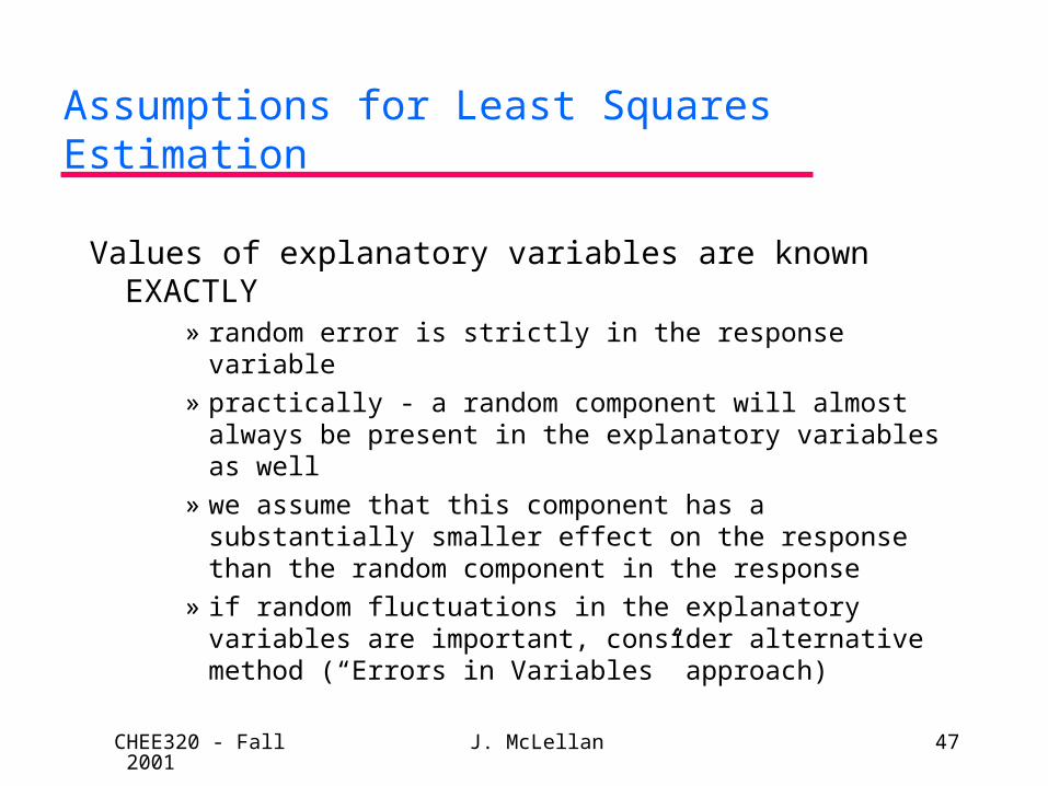
Assumptions for Least Squares Estimation
Values of explanatory variables are known EXACTLY» random error is strictly in the response variable» practically - a random component will almost always be
present in the explanatory variables as well» we assume that this component has a substantially
smaller effect on the response than the random component in the response
» if random fluctuations in the explanatory variables are important, consider alternative method (“Errors in Variables” approach)

CHEE320 - Fall 2001
J. McLellan 48
Assumptions for Least Squares Estimation
The form of the equation provides an adequate representation for the data
» can test adequacy of model as a diagnostic
Variance of random error is CONSTANT over range of data collected
» e.g., variance of random fluctuations in thickness measurements at high temperatures is the same as variance at low temperatures
» data is “heteroscedastic” if the variance is not constant - different estimation procedure is required
» thought - percentage error in instruments?

CHEE320 - Fall 2001
J. McLellan 49
Assumptions for Least Squares Estimation
The random fluctuations in each measurement are statistically independent from those of other measurements
» at same experimental conditions» at other experimental conditions» implies that random component has no “memory”» no correlation between measurements
Random error term is normally distributed» typical assumption» not essential for least squares estimation» important when determining confidence intervals, conducting
hypothesis tests

CHEE320 - Fall 2001
J. McLellan 50
Least Squares Estimation - graphically
least squares - minimize sum of squared prediction errors
response (solder thickness)
T
o
o
o
o
oo deterministic
“true”relationship
prediction error“residual”
CHEE320 - Fall 2001
J. McLellan 51
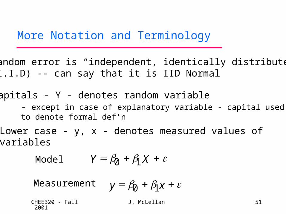
More Notation and Terminology
Random error is “independent, identically distributed” (I.I.D) -- can say that it is IID Normal
Capitals - Y - denotes random variable- except in case of explanatory variable - capital used
to denote formal def’n
Lower case - y, x - denotes measured values ofvariables
Model
Measurement
Y X 0 1
y x 0 1
CHEE320 - Fall 2001
J. McLellan 52
More Notation and Terminology
Estimate - denoted by “hat”» examples - estimates of response, parameter
Residual - difference between measured and predicted response
, y 0
e y y

CHEE320 - Fall 2001
J. McLellan 53
Least Squares Estimation
Find the parameter values that minimize the sum of squares of the residuals over the data set:
Solution » solve conditions for stationary point (“normal equations”)» derivatives with respect to parameters = 0» obtain analytical expressions for the least squares
parameter estimates
e y xii
Ni i
i
N2
10 1
2
1 [ ( )]

CHEE320 - Fall 2001
J. McLellan 54
Least Squares Parameter Estimates
( )
0 1
11
2
1
2
y x
x y nx y
x n x
i ii
N
ii
N
Note that the parameter estimates are functions of BOTH the explanatory variable values and the measuredresponse values --> functions of “noisy data”

CHEE320 - Fall 2001
J. McLellan 55
Diagnostics - Graphical
Basic Principle - extract as much trend as possible from the data
Residuals should have no remaining trend - » with respect to the explanatory variables» with respect to the data sequence number» with respect to other possible explanatory variables
(“secondary variables”)» with respect to predicted values

CHEE320 - Fall 2001
J. McLellan 56
Graphical Diagnostics
Residuals vs. Predicted Response Values
residualei
yi
*
*
*
*
**
*
*
*
** *
*
*
- even scatter over range of prediction
- no discernable pattern
- roughly half the residualsare positive, half negative
DESIRED RESIDUAL PROFILE

CHEE320 - Fall 2001
J. McLellan 57
Graphical Diagnostics
Residuals vs. Predicted Response Values
residualei
yi
*
**
*
*
*
*
*
*
** *
*
*
outlier lies outsidemain body of residuals
RESIDUAL PROFILE WITH OUTLIERS

CHEE320 - Fall 2001
J. McLellan 58
Graphical Diagnostics
Residuals vs. Predicted Response Values
residualei
yi**
*
*
**
*
*
*
** *
**
variance of the residualsappears to increasewith higher predictions
NON-CONSTANT VARIANCE
*
*
*
*
CHEE320 - Fall 2001
J. McLellan 59
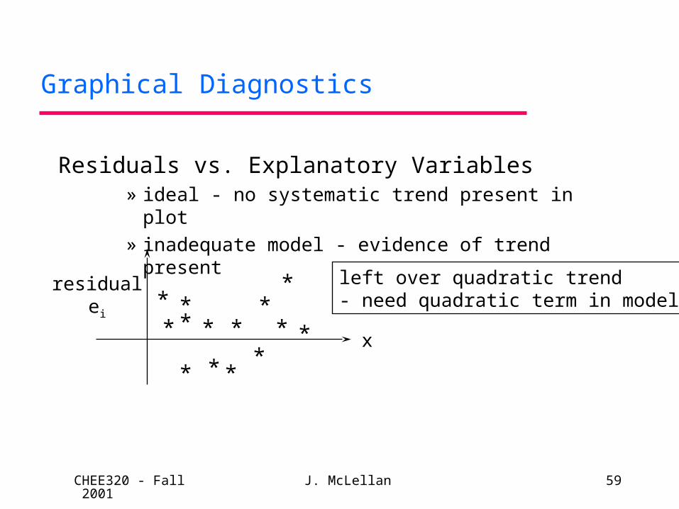
Graphical Diagnostics
Residuals vs. Explanatory Variables» ideal - no systematic trend present in plot» inadequate model - evidence of trend present
residualei
** *
*
**
* *
** *
*
*
*x
left over quadratic trend - need quadratic term in model

CHEE320 - Fall 2001
J. McLellan 60
Graphical Diagnostics
Residuals vs. Explanatory Variables Not in Model» ideal - no systematic trend present in plot» inadequate model - evidence of trend present
residualei
*
* **
** * *
** *
*
*
*w
systematic trendnot accounted for in model- include a linear term in “w”

CHEE320 - Fall 2001
J. McLellan 61
Graphical Diagnostics
Residuals vs. Order of Data Collection
residualei
** ** *
*
* * ** *
*
**
t
*
** **
** *
* ***
*t
residualei
failure to account for time trendin data
successive random noise components are correlated - consider more complex model- time series model for random component?
CHEE320 - Fall 2001
J. McLellan 62
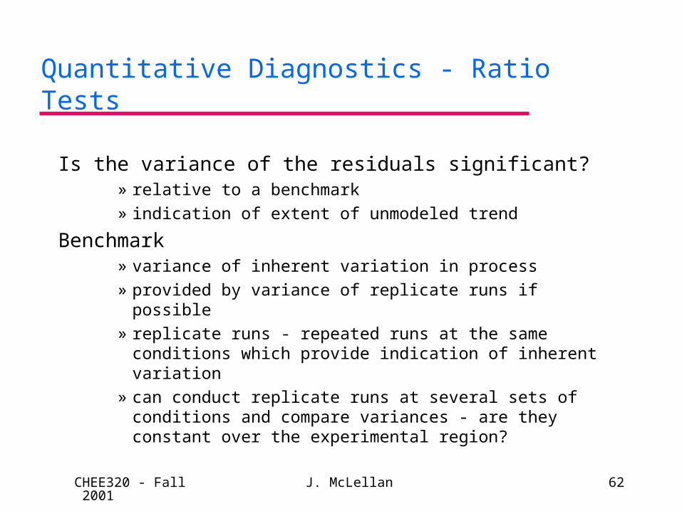
Quantitative Diagnostics - Ratio Tests
Is the variance of the residuals significant?» relative to a benchmark» indication of extent of unmodeled trend
Benchmark» variance of inherent variation in process » provided by variance of replicate runs if possible» replicate runs - repeated runs at the same conditions
which provide indication of inherent variation» can conduct replicate runs at several sets of conditions
and compare variances - are they constant over the experimental region?

CHEE320 - Fall 2001
J. McLellan 63
Quantitative Diagnostics - Ratio Tests
Residual Variance Ratio
Mean Squared Error of Residuals (Var. of Residuals):
s
s
Mean Squared Error of Residuals MSE
sresiduals
inherent inherent
2
2 2 ( )
s MSE
e
Nresiduals
ii
N
2
2
12

CHEE320 - Fall 2001
J. McLellan 64
Quantitative Diagnostics - Ratio Tests
Is the ratio significant?
- compare to the F-distribution
Why?» ratio is the ratio of sums of squared normal r.v.’s» squared normal r.v.’s have a chi-squared distribution» ratios of chi-squared r.v.’s have an F-distribution
Degrees of freedom » number of statistically independent pieces of information used to
calculate quantities» degrees of freedom of MSE is N-2, where N is number of data points» d. of f. for inherent variance is M-1, where M is number of data points
used to estimate inherent variance

CHEE320 - Fall 2001
J. McLellan 65
Quantitative Diagnostics - Ratio Tests
Interpretation of Ratio» if significant, then model fit is not adequate as the
residual variation is large relative to the inherent variation» “still some signal to be accounted for”
Example - Solder Thickness» previous data - variance is 102.2 (24 degrees of
freedom)» residual variance (MSE)
MSE
eii
N
2
110 2
10830
8135 38
..

CHEE320 - Fall 2001
J. McLellan 66
Quantitative Diagnostics - Ratio Tests
The ratio is:
Compare to
The residual variance is NOT statistically significant, and no evidence of inadequacy is detected.
MSE
sinherent2
13538102 2
132 ..
.
F8 24 0 95 2 36, , . .
Fn1,n2
2.36^
1.32
5% of values occur outsidethis fence( area of tail is 0.05)

CHEE320 - Fall 2001
J. McLellan 67
Quantitative Diagnostics - Ratio Tests
Mean Square Regression Ratio
- is the variance described by the model significant relative to an indication of the inherent variation?
Variance described by model:
MSR
y y
py y
ii
N
ii
N
( )
( )
2
1 2
11

CHEE320 - Fall 2001
J. McLellan 68
Quantitative Diagnostics - Ratio Test
Test Ratio:
is compared against F1,N-2,0.95
Conclusions?– ratio is statistically significant --> significant trend has been
modeled– ratio is NOT statistically significant --> significant trend has
NOT been modeled, and model is inadequate in its present form
MSRMSE

CHEE320 - Fall 2001
J. McLellan 69
Quantitative Diagnostics - Ratio Tests
Notes on MSR/MSE Ratio Test:» MSE provides a rough indication of inherent variation» use of MSE as indication of inherent variation assumes
model form is adequate» MSE contains effects of 1) background variation, 2)
model specification error» MSR/MSE ratio is frequently compared against F at the
75% level to guard agains erroneous rejection of an adequate model
» this is a “coarse” test of adequacy!

CHEE320 - Fall 2001
J. McLellan 70
Analysis of Variance Tables
The ratio tests involve dissection of the sum of squares:
{SSR
y yii
N
( )2
1
SSE
y yi ii
N
( )2
1
TSS y yii
N
( )2
1

CHEE320 - Fall 2001
J. McLellan 71
Analysis of Variance (ANOVA) for Regression
Sourceof
Variation
Degreesof
Freedom
Sum ofSquares
MeanSquare
F-Value p-value
Regression 1 SSR MSR=SSR/1=SSR
F=MSR/MSE
p
Residuals N-2 SSE MSE=SSE/(N-2)
Total N-1 TSS

CHEE320 - Fall 2001
J. McLellan 72
Quantitative Diagnostics - R2
Coefficient of Determination (“R2 Coefficient”)» square of correlation between observed and predicted
values:
» relationship to sums of squares:
» values typically reported in “%”, i.e., 100 R2
» ideal - R2 near 100%
R corr y y2 2[ ( , )]
RSSE
TSS
SSR
TSS2 1

CHEE320 - Fall 2001
J. McLellan 73
Example - Solder Data
SUMMARY OUTPUT
Regression StatisticsMultiple R 0.920001R Square 0.846402Adjusted R Square0.827203Standard Error9.399193Observations 10
ANOVAdf SS MS F Significance F
Regression 1 3894.602 3894.602 44.0841 0.000163Residual 8 706.7586 88.34482Total 9 4601.361
fairly high - accounting for trend
correlation coefficient which has notbeen squared
large ratio which is stronglysignificant - we are picking upsignificant trend

CHEE320 - Fall 2001
J. McLellan 74
Properties of the Parameter Estimates
( )
0 1
11
2
1
2
Y x
x Y nxY
x n x
i ii
N
ii
N
Let’s look at the formal defn’s. of the parameter estimates:
x’s have been left in lower case only to emphasizethe fact that they aren’t random variables

CHEE320 - Fall 2001
J. McLellan 75
Properties of the Parameter Estimates
The eqns. for the parameter estimates are of the form:
i.e., linear combinations of random variables.
If Y’s are normally distributed, then linear combinations of y’s are normally distributed, and parameter estimates are normally distributed
1 1 1
0 1
k Y k Y k Y
Y k
N N m
The parameter estimates are STATISTICS

CHEE320 - Fall 2001
J. McLellan 76
Properties of the Parameter Estimates
Mean:
E E
x Y NxY
x Nx
x E Y NxE Y
x Nx
x x Nx x
x Nx
i ii
N
ii
N
i ii
N
ii
N
i ii
N
ii
N
{ }
{ } { }
{ } { }
11
2
1
2
1
2
1
2
0 11
0 1
2
1
21

CHEE320 - Fall 2001
J. McLellan 77
Properties of the Parameter Estimates
Similarly,
Conclusion?» the value expected on average for the least squares
parameter estimates is the true value of the parameter» if we repeated the data collection/model estimation
exercise an infinite number of times, we would obtain the true parameter estimates “on average”
E{ } 0 0
The least squares parameter estimates are UNBIASED

CHEE320 - Fall 2001
J. McLellan 78
Variance of the Parameter Estimates
Since the parameter estimates are unbiased,
Using the definitions for the parameter estimates:
Var E
Var E
( ) {( ) }
( ) {( ) }
0 0 0
2
1 1 12
VarN
x
x x
Var
x x
ii
N
ii
N
( )
( )
( )
( )
02
2
1
2
12
1
2
1
is the varianceof the random noise componentin the measurements
2

CHEE320 - Fall 2001
J. McLellan 79
Making Inferences About Parameters
Inferences - decisions - can be made about the true values of the parameters by taking into account the variation in the parameter estimates
» hypothesis tests» confidence limits
The inference requires knowledge of the random behaviour - sampling behaviour - of the parameter estimate statistics
» distribution - for Normally distributed random components in the data, the parameter estimates are Normal random variables

CHEE320 - Fall 2001
J. McLellan 80
Inferences for Parameters
We follow exactly the same argument » use the estimate of the random noise variance to
estimate the variance of the parameter estimates using the expression for parameter estimate variance
» the true value of the parameter is the mean of the parameter estimate
s sN
x
x x
ss
x x
ii
N
ii
N
( )
( )
0
1
2 22
1
2
22
1
2
1

CHEE320 - Fall 2001
J. McLellan 81
Confidence Intervals for Parameters
For intercept:
For slope:
Degrees of freedom for the t-distribution:» comes from the degrees of freedom of the estimate of
the random noise variance» option 1 - use external estimate of noise variance -
“inherent” variance that we had before» option 2 - use mean square error of the residuals (MSE)
- sometimes referred to as the “standard error”
, / 0 2 0t s
, / 1 2 1t s

CHEE320 - Fall 2001
J. McLellan 82
Example - Solder Thickness
Using the MSE to estimate the inherent noise variance:
MSESSEN
s MSE
s sx
x x
s s
x x
e
e
ii
e
ii
2706 7610 2
88 35
88 35 9 399
110
40 287
10169
0
1
2
2
1
10
2
1
10
..
. .
( )
.
( )
.
x
xii
236 7
563 3352
1
10
.
,

CHEE320 - Fall 2001
J. McLellan 83
Example - Solder Thickness
95% Confidence Limits
For intercept:
For slope:
4581 40 287 4581 2 306 40 287
4581 92 9 3652 551
10 2 0 025. ( . ) . . ( . )
. . [ . , ]
, .
t
1127 0169 1127 2 306 0169
1127 0 390 152 0 7410 2 0 025. ( . ) . . ( . )
. . [ . , . ], .t

CHEE320 - Fall 2001
J. McLellan 84
Example - Solder Thickness
Interpretation - » slope parameter is significantly non-zero» intercept parameter is significantly non-zero» retain both terms in the model

CHEE320 - Fall 2001
J. McLellan 85
Correlation of the Parameter Estimates
Note that
I.e., the parameter estimate for the intercept depends linearly on the slope!
» the slope and intercept estimates are correlated
0 1 Y x
changing slope changespoint of intersection withaxis because the line must go through the centroid of thedata

CHEE320 - Fall 2001
J. McLellan 86
Getting Rid of the Covariance
Let’s define the explanatory variable as the deviation from its average:
Z X X
0
11
2
1
Y
z Y
z
i ii
N
ii
N
Least Squares parameterestimates:
- note that now there is no explicitdependence on the slope valuein the intercept expression
- average of z is zero

CHEE320 - Fall 2001
J. McLellan 87
Getting Rid of the Covariance
In this form of the model, the slope and intercept parameter estimates are uncorrelated
Why is lack of correlation useful?» allows indepedent decisions about parameter estimates
» decide whether slope is significant, intercept is significant individually
» “unique” assignment of trend• intercept clearly associated with mean of y’s
• slope clearly associated with steepness of trend
» correlation can be eliminated by altering form of model, and choice of experimental points