Vorlesung Grundlagen der Bioinformatik gobics.de/lectures/ss07/grundlagen

Checking Landau's "Grundlagen" in the Automath system
Benthem Jutting, van, L.S.
DOI:10.6100/IR23183
Published: 01/01/1977
Document VersionPublisher’s PDF, also known as Version of Record (includes final page, issue and volume numbers)
Please check the document version of this publication:
• A submitted manuscript is the author's version of the article upon submission and before peer-review. There can be important differencesbetween the submitted version and the official published version of record. People interested in the research are advised to contact theauthor for the final version of the publication, or visit the DOI to the publisher's website.• The final author version and the galley proof are versions of the publication after peer review.• The final published version features the final layout of the paper including the volume, issue and page numbers.
Link to publication
Citation for published version (APA):Benthem Jutting, van, L. S. (1977). Checking Landau's "Grundlagen" in the Automath system Amsterdam:Mathematisch Centrum DOI: 10.6100/IR23183
General rightsCopyright and moral rights for the publications made accessible in the public portal are retained by the authors and/or other copyright ownersand it is a condition of accessing publications that users recognise and abide by the legal requirements associated with these rights.
• Users may download and print one copy of any publication from the public portal for the purpose of private study or research. • You may not further distribute the material or use it for any profit-making activity or commercial gain • You may freely distribute the URL identifying the publication in the public portal ?
Take down policyIf you believe that this document breaches copyright please contact us providing details, and we will remove access to the work immediatelyand investigate your claim.
Download date: 17. Sep. 2018


CHECKING LANDAU'S ''GRUNDLAGEN'' IN THE
AUTOMATH SYSTEM

CHECKING LANDAU'S ''GRUNDLAGEN'' IN THE
AUTOMATH SYSTEM
PROEFSCHRIFT
TER VERKRIJGING VAN DE GRAAD VAN DOCTOR IN DE
TECHNISCHE WETENSCHAPPEN AAN DE TECHNISCHE
HOGESCHOOL EINDBOVEN 1 OP GEZAG VAN DE RECTOR
MAGNIFICUS, PROF.DR. P. VAN DER LEEDEN, VOOR
EEN COMMISSIE AANGEWEZEN DOOR HET COLLEGE VAN
DEKANEN IN HET OPENBAAR TE VERDEDIGEN OP
DINSDAG 1 MAART 1977 TE 16.00 UUR.
door
L.S. VAN BENTHEM JUTTING
GEBOREN TE BUSSUM

Dit proefschrift is goedgekeurd
door de promotoren
Prof.dr. N.G. de Bruijn
en
Prof.dr. w. Peremans

Preface
This thesis contains an account of the translation and verification of
Landau's "Grundlagen der Analysis", a book on elementary mathematics [L],
in the formal language A!JT-QE, a language of the AUTOMATH family.
AUTOMATH languages are intended to be used for formalizing mathematics
in such a precise way that correctness can be checked mechanically (e.g. by
a computer) •
The translation itself is presented in L.S. Jutting, A translation of
Landau's "Grundlagen" in AUTOMATH [J]. It consists of about 500 pages, and
therefore it is not reproduced here, apart from two fragments (see appendi
ces 4 and 7).
Acknowledgel!lE!nts
I want to thank all my. fellow-workers in the AUTOMATH project for their
help, in the form of ideas and advice, of material assistance and moral sup
port.
I want to thank my family for putting up with my preoccupation, in par
ticular during this last half year.
I want to thank Mrs. Marese Wolfs and Mrs. Lieke Janson ·for typing
these pages.
Contents
0. INTRODUCTION
0.0. The AUTOMATH languages
0.1. The AUTOMATH project and its motivation
0.2. The book translated
0.3. The language of the translation
1. PREPARATION
2.
1.0. The presupposed logic
1.2. The representation of logic in AUT-QE
1.3. Account of the PN-lines
1.4. Development of concepts and theorems in Landau's logic
TRANSLATION
2,0. An abstract of Landau's book
2.1. Deviations from Landau's text
2.2. The translation of "Kapitel 1"
2.3. The translation of "Kapitel 2"
2.4. The translation of "Kapitel 3"
2.5. The translation of "Kapitel 4"
2.6. The alternative version of chapter 4
2.7. The translation of "Kapitel 5"
3. VERIFICATION
3.0. Verification of the text
3,1, Controlling the strategy of the program
3.2. Shortcomings in the verifying program
3,3. Excerpting
4. CONCLUSIONS
4.0. Formalization of logic in AUTOMATH
4. 1. The language
4.2. comments on the translation
page
1
2
2
4
8
9
11
14
16
23
24
24
25
27
27
30
32
33
33
35
39
44
Appendix 1, A description of AUTOMATH and some aspects of its
language theory by D.T. van Daalen
1, Introductory remarks
2, Informal description of AUTOMATH
3. Mathematics in AUTOMATH: Propositions as types
4. Extension of AUT-68 to AUT-QE
5, A formal definition of AUT-QE
6. Some remarks on language theory
Appendix 2, The paragraph system
Appendix 3. PN-lines from the preliminaries
Appendix 4. Excerpt for "Satz 27"
Appendix 5, Two shortcomings of the verifying program
Appendix 6. Example of a text in AUT-68
Appendix 7. Excerpt for "Satz 1", "Satz 2" and "Satz 3"
Appendix 8. Example of a text in AUT-68-SYNT
Appendix 9. AUT-SYNT
References
48
49
50
59
62
65
71
78
84
86
99
101
107
110
117
120
1
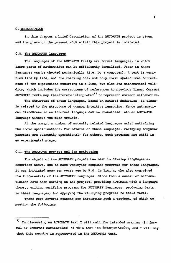
0. INTRODUCTION
In this chapter a brief description of the AUTOMATH project is given,
and the place of the present work within this project is indicated.
0. 0. The AUTOMATH languages
The languages of the AUTOMATH family are formal languages, in which
large parts of mathematics can be ef~iciently formalized. Texts in these
languages can be checked mechanically (i.e. by a computer). A text is veri
fied line by line, and the checking does not only cover syntactical correct
ness of the expressions occurring in a line, but also its mathematical vali
dity, which includes the correctness of references to previous lines. Correct
AUTOMATH texts may thereforebe interpreted*) to represent correct mathematics,
The structure of these languages, based on natural deduction, is close
ly related to the structure of common intuitive reasoning. Hence mathemati
cal discourses in an informal language can be translated into an AUTOMATE
language without too much trouble.
At the moment a number of mutually related languages exist satisfying
the above specifications. For several of these languages, verifying computer
programs are currently operational; for others, such programs are still in
an experimental stage.
0.1. The AUTOMATE project and its motivation
The object of the AUTOMATH project has been to develop languages as
described above, and to make verifying computer programs for these languages.
It was initiated some ten years ago by N.G. de Bruijn, who also conceived
the fundamentals of the AUTOMATE languages. Since then ·a number of mathema
ticians have been working on the project, providing AUTOMATE with a language
theory, writing verifying programs for AUTOMATE languages, producing texts
in these languages, and applying the verifying programs to these texts.
There were several reasons for ~nitiating such a project, of which we
mention the following:
*) In discussing an AUTOMATE text I will call the intended meaning (in for~
mal or informal mathematics) of this text its inte:r>pretati.on, and I will say
that this meaning is Nproesented in the AUTOMATE text.

2
i) Mechanical verification will increase the reliability of certain kinds
of proofs. A need for this may be felt where a proof is extremely long,
complicated and tedious, and where it is difficult to break it down in
to intuitively plausible partial results; or where in proofs results of
others are used, so that misinterpretations become possible.
ii) Mechanically verifiable languages set a standard by which informal lan
guage may be measured, and may thereby have an influence on the use of
language in mathematics generally.
iii) The use of such languages gives an insight into the structure of mathe
matical texts, and makes it possible to compare the complexity, in se
veral respects, of mathematical concepts and proofs. As a consequence
projects of this kind may have in the long run a favourable influence
on the teaching of mathematics.
A further motive, for the author, was that the Work involved in the
project appealed to him.
More information on the AUTOMATH project, its objectives, motivation
and history can be found in [dB].
0.2. The book translated
At an early stage of the AUTOMATH project the need was felt to trans
late an existing mathematical text into an AUTOMATH language, first, in or
der to acquire experience in the use of such a language, and secondly, to
investigate to what extent mathematics could be represented in AUTOMATH in
a natural way.
As a text to be translated, the book "Grundlagen der Analysis" by
E. Landau [L] was chosen. This book seemed a good choice for a number of
reasons: it does not presuppose any mathematical theory, and it is written
clearly, with much detail and with a rather constant degree of precision.
For a short description of the contents of Landau's book see 2.0.
0.3. The language of the translation
The language into which Landau's book has been translated is AUT-QE.
A detailed description and a formal definition of this language is given in
[vD]. As this paper is fundamental to the following monograph and not easi
ly obtainable, it has been added as appendix .1. I will use the notations
introduced there whenever necessary. Where in the following text ~ concept
introduced in [vD] is used for the first time, it will be displayed in
italics, with a reference to the section in [vD] where it occurs.
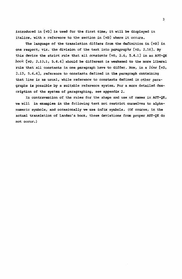
3
The language of the translation differs from the definition in [vD] in
one respect, viz. the division of the text into paragraphs [vo, 2,16], By
this device the strict rule that all aonstants [vo, 2.6, 5,4.1] in an AUT-QE
book [vo, 2.13,1, 5.4.4] should be different is weakened to the more liberal
rule that all constants in one paragraph have to differ. Now, in a Line [vD,
2.13, 5.4.4], reference to constants defined in the paragraph containing
that line is as usual, while reference to constants defined in other para
graphs is possible by a suitable reference system. For a more detailed des
cription of the system of paragraphing, see appendix 2.
In contravention of the rules for the shape and use of names in AUT-QE,
we will in examples in the following text not restrict ourselves to alpha
numeric symbols, and occasionally we use infix symbols. (Of course, in the
actual translation of Landau's book, these deviations from proper AUT-QE do
not occur.)

4
1 • PREPARATION
In this chapter the logic which Landau presupposes is analysed and its
representation in AUT-QE is described.
1.0. The presupposed logic
In his "Vorwort fiir den Lernenden" Landau states: "Ich setze loqisches
Denken und die deutsche Sprache als bekannt voraus". Clearly, in the trans
lation AUT-QE should be substituted for "die deutsche Sprache", rhe proper
interpretation of "loqisches denken" must be inferred from Landau's use of
logic in his text.
This appears to be a kind of informal second (or higher) order predi
cate logic with equality. In the following some characteristics of Landau's
logic will be discussed, and illustrated by quotations from his text.
i) Variables have well defined ranges which are not too different from
types [vD, 2,2] in AUT-QE, Cf.:
-On the first page of "Kapitel 1": "Kleine lateinische Buchstaben be
deuten in diesem Buch, wenn nichts anderes gesagt wird, durchweg na
tiirliche Zahlen".
- In "Kapitel 2, § 5": Grosze lateinische Buchstaben bedeuten durchweg,
wenn nichts anderes gesagt wird, rationale Zahlen".
ii) Predicates have restricted domains, which again can be interpreted as
types in AUT-QE. Cf.:
- "Sa:tz 9: Sind x und y gegeben, so liegt genau eine der Ftille vor:
1) X = Y•
2) Es gibt ein u mit x == y + u ••• " etc.
It is clear that u (being a lower case letter) is a natural number,
or u E nat.
- "Definition 28: Eine Menge von rationalen Zahlen heiszt ein Schnitt,
wenn .•• ".
Here it is apparent that beinq a "Schnitt" is a predicate on the type
of sets of rational numbers.
iii) When, for a predicate P, it has been shown that a unique x exists for
which P holds, then "the x such that P" is an object. Cf.:
- "Satz 4, zugleich Definition 1: Auf genau eine Art l!szt sich jedem
Zahlenpaar x,y eine natiirliche Zahl, x +y genannt, so zuo:rdnen.
dasz •••• x +y heiszt die Summe von x und y".

5
- "Satz 101: Ist X > Y so hat X+ U = Y genau eine LOsung u.
Definition 23: Dies U heiszt X - Y".
iv) The theory of equivalence classes modulo a given equivalence relation,
whereby such classes are considered as new objects, is presupposed by
Landau. Cf.:
- The text preceding "Satz 40": "Auf Grund der Satze 37 bis 39 zerfal-
len alle BrQche in Klassen, so x1 Yt
dasz - - - dann und nur dann, wenn x2 Y2 x1 Y1
- und - derselben Klasse angehOren". x2 Y2
- "Definition 16: Unter eine rationale Zahl versteht mann die Menqe
aller einem festen Bruch aquivalenten BrQche (also eine Klasse im
Sinne des § 1)".
v) The concepts "function" and "bijective function" are vaguely described.
Cf.:
- "Satz 4" (see iii) above).
- "Satz 274: Ist x < y so kOnnen die m ~ x nicht auf die n ~ y einein-
deutig bezogen werden".
- "Satz 275: Es sei x fest, f(n) far n ~ x definiert. Dann gibt es ge
nau ein fQr n ~ x definiertes gx(n) mit folqenden Eigenschaften ••• "
followed by the "explanation"; "Unter definiert verstehe ich: als
komplexe Zahl definiert". This explanation might be interpreted to
indicate the typing of the functions f and g.
vi) Landau defines and uses partial functions. Cf.:
- "Definition 14: Das beim Beweise des Satzes 67 konstruierte spezielle ul xl Yt - heiszt-- - ••• ". Here the construction, and therefore the de-u2 x2 Y2 x y finition, only applies if _! > _!
x2 Y2
- "Definition 56: Das Y des Satzes 204 heiszt i ". This definition de-
pends upon H ' 0.
- "Definition 71", where Landau states explicitly: "Nicht definiert
1st xn also lediglich far x .. 0, n ~ 0".
- "Satz 155: Beweis: II) Aus X > Y folgt X "" (X- Y) + Y".
- "Satz 240: Ist y' 0 so ist!.. y = x". y n
- "Satz 291: Es sei n,. 0 oder x1 'I O, x2 ' 0. Dann 1st <x1.x2) =
n n " = x1 .x2
6
J:n these last three examples we see "generalised implications": the
terms occurring in the consequent are meaningful only if the antece
dent is taken to be tr~e. A similar situation will be encountered in
vii}.
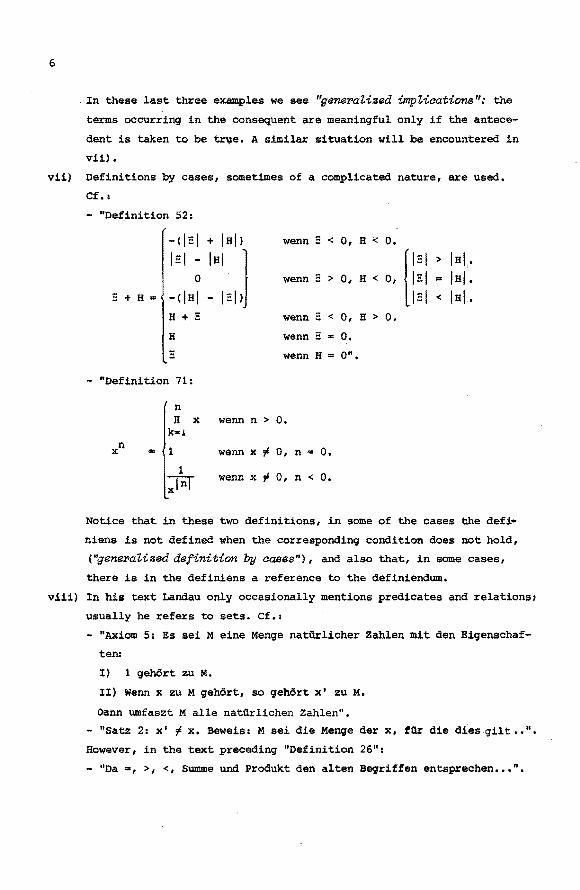
vii} Definitions by cases, sometimes of a complicated nature, are used.
Cf.:
- "Definition 52:
wenn E < 0 1 H < 0.
E + H = r > I al,. wenn E > 0 1 H < o, 1::1 I al.
1=1 < I al. H + E wenn E < o, B > 0,
H wenn E = o. wenn B = 0".
- "Definition 71:
n n X wenn n > o.
k=! n
1 'F o, o. X = wenn x n =
1 ;. o, n < 0. N wenn x X
Notice that in these two definitions, in some of the cases the defi•
niens is not defined when the corresponding condition does not hold,
("gene:r-aZised definition by caeee"), and also that, in some cases,
there is in the definiens a reference to the definiendum,
viii} In his text Landau only occasionally mentions predicates and relations;
usually he refers to sets. Cf.:
- "AXiom 5: Es sei M eine Menge nat'Grlicher Zahlen mit den Eigenschaf
ten:
I) 1 gehdrt zu M.
II) Wenn x zu M geh6rt, so geh6rt x' zu M.
oann umfaszt M alle nattlrlichen Zahlen".
- "Satz 2: x' '/' x. Beweis: M sei die Menge der x, fiir die dies qilt. •"•
However, in the text preceding "Definition 26":
- "Da =, >, <, Summe und Produkt den alten Begriffen entsprechen ... ".
7
ix) Landau considers (ordered) pairs of objects. In chapter 2 the compo
nents of such pairs remain clearly visible in their names: he does not
refer to "the pair x with components x1 ana x2", but only to "the pair
x1,x2". Nevertheless it is clear from his worCis that he considers such
a pair as one object. Cf.: x1
- "Definition 7: Unter einem Bruch - versteht man Clas Paar Cler nat1irx2
lichen Zahlen x1 ,x2 (in dieser Reihenfolge)",
xl Y1 - "Definition 8: - - - wenn x y = y x ". x 2 y 2 1 2 1 2
In chapter 5 however, variables for pairs ave used. Cf.:
-"Definition 57: Eine komplexe Zahl ist ein Paar re!ller Zahlen : 1,:2 (in bestimmter Reihenfolge). Wir bezeichnen die komplexe Zahl mit
[E1,E2]".
This definition is immeCiiately followed by
- "Kleine deutsche Buchstaben bedeuten durchweg komplexe Zahlen" •
The two notations are linked in the following way:
- "Definition 60: Ist X= [E1,E2], y = [H1,a2J, so ist
x + y = [E1 + E2 ,a1 + a2J". x) Finally it should be pointed out that some of Landau's proofs ana re
marks tend to a kind of intuitive reasoning which is noteasilyrepresen
ted in a formal system.
A first example of this is the treatment of equality in "Kapitel 1,
s 1".
- "Ist x gegeben und y geqeben, so sinCI entweder x und y dieselbe Zahl;
Clas kann man auch x = y schreiben; oder x unCI y nicht Clieselbe Zahl;
das kann men auch x ~ y schreiben.
Hiernach gilt aus rein loqischen GrOnden:
1) x == x fdr jedes x.
2) A us x = y folgt y = x.
3) Aus x = y, y = z folqt x = z".
Here it seems that Landau derives the properties of equality from re
flection on the properties of a mathematical structure. They are not
theorems or axioms but intuitively true statements. Substitutivity of
equal objects, though used frequently in the proofs of subsequent theo
rems, is never mentioned.
Other examples of proofs with intuitive components may be found where
Landa~, in a glance, takes in a complex logical situation. Cf.:
8
- "Satz 16: Aus x s y, y < z oder x < y, y s z folgt x'< z. Beweis:
Mit dem Gleichheitszeichen in der Voraussetzung klar; sonst durch
Satz 15 erlediqt".
- "Satz 20: Aus x + z > y + z bzw. x + z y + z bzw. x + z < y + z
folgt x > y bzw. x = y bzw. x < y.
Beweis: Folgt aus Satz 19 da die drei Fllle beide Male s!ch aus
schl!eszen und alle Moglichkeiten erschopfen".
A somewhat different example, which involves what might be called
"metalogic", is the text preceding "Definition 26", where it .is indi
cated how a number of theorems might be proved, without actually pro
ving them, I will return to this in 2.1 viii).
1.2. The representation of logic in AUT-QE
The logic considered by Landau to be "logisches Denken", as described
in the previous section, has been formalized in the first part of the
AUT-QE book, called "preliminaries", which, unlike the other parts, does
not correspond to an actual chapter of Landau's book.
A possible way of coding logic in AUT-QE has been described in [vD,
3,4]. In addition to this description we stress a few points on the inter
pretation of AUT-QE lines [vo, 2.13, 5.4.4]. Adopting the terminology intro
duced in [Z] we shall call expressions of the form [x1,a1J •• ,[~,ak] ~ (with k ~ 0) (i.e. t-expressions of degree 1) lt-erop~eeione and ex
pressions of the form [x1,a1J ••• [xk,ak] ~ (again with k ~ 0) 1p-erop~ea
sione. Expressions having lt- and lp-expressions as their types, will be
called 2t-exp~eseione and 2p-eoop~essions~ respectively. Finally, 3t- and
3p-exp~eesions have 2t- and 2p-expressions as their types.
Now a 2t-expression will be used to denote a type (or "class"). If
its type is an abst~aotion erep~eeeion [vo, 2.8, 5.4.2] then it denotes a
type of functions. A 2p-expression denotes a proposition or a predicate. A
3t-expression denotes an object {of a certain type) and a 3p-expression a
proof (of a certain proposition).
The interpretation of an AUT-QE line having a certain shape (EB-tine~
PN-line or abbreviation line [vo, 2.13, 5.4.4]) will depend on its catego
ry part [vD, 2.13.1] being a lt-, 1p-, 2t- or 2p-expression. So we arrive
at the following refinement of the scheme in [vD, 4.5].

9
Shape of the line: Category-part
it-expression lp-expression 2t-expression 2p-expression
EB-line
PN-line
Abbreviation
line
introduces
a type
varial:lle
introduces
a primitive
type con
stant
defines a
type in
terms of
known con
cepts
introduces a
proposition
or predicate
varial:lle
introduces an
object varia
ble (of the
stated type)
introduces
the stated
proposition
as an assump·
tion
introduces a introduces a introduces
primitive primitive ob- the stated
proposition
or predicate
constant
defines a
proposition
or predicate
in terms of
known con
cepts
ject (of the proposition
stated type) as an axiom
defines an
object (of
the stated
type) in
terms of
known con
cepts
proves the
stated pro
position as
a theorem
In the above scheme it is apparent that, if the category part of a line is
a 2p-expression, then the interpretation of that line is an assertion. But
also if the category part is a 2t-expression a the interpretation has an
assertional aspect• the line does not only introduce a new name for an ob
ject (as a variable, or a primitive or defined constant) but also asserts
that this object has the type a.
1,3, Account of the PN-lines
Here I will give a survey of the primitive concepts and axioms (PM
lines) occurring in the preliminary AUT-QE text. A mechanically produced
list of these axioms appears as appendix~. In this list the PN-lines appear
numbered. References in parentheses below will refer to these numbers.
i) Axioms for contradiction.
Contradiction is postulated as a primitive proposition (1), the double
negation law as an axiom (2).

10
ii) Axioms for equality.
Given a type S 1 equality is introduced as a primitive relation on S
(3) 1 with axioms for reflexivity (4) and for substitutivity (5) (i.e.
if X=y 1 and if P is a predicate on S which holds at X 1 then P
holds at y ). Moreover there is an axiom stating extensionality for
functions ( 8) •
The notion of equality so introduced is called book-equality (cf. [vD 1
3.6]) in contrast to definitional equality of expressions. ([vD 1 2.12 1
5.5.6]).
iii) Axioms for individuals.
Given a type S , a predicate P on
at a unique X f S , the object ind
S , and a proof that P holds
(for individual) is a primitive
object (6), to be interpreted as "the X for which P holds". An
axiom states that ind satisfies P (7).
iv) Axioms for subtypes.
Given a type S and a predicate P on S , the type OT (for own
type, i.e. the subtype of S associated with P ) is a primitive typer
(9). For u f OT we have a primitive object in{u) f S (10), and an
axiom stating that the function [u,OTJin(u) is injective (12). More
over there are axioms to the effect that the images under this func
tion are just those X f S for which P holds ((11) and (12)).
v) Axioms for products {of types).
Given types S and T the type pairtype (the type of pairs (x,y)
with X f S and y f T ) is introduced as a primitive type (14). For
p f pairtype we have the projections first{p) f S and second(p) fT
as primitive objects ((16) and (17)), and conversely, for X f S and
y f T we have patr(x,y) as a primitive object in pairtype (15).
Next there are three axioms stating that pair(first{p).second{p))•p,
first(pair(x,y))=x and second(pair(x,y))=y (where= refers to book
equality as introduced in H)) ( (19), (20) and (21)).
(Note( If a type U containinq just two objects is available, and if
S is a type, the type of pairs (X,y) with X f S and y f S may
be defined alternatively as the function type [X,U]S • In the trans
lation this was done at the end of chapter 1, where we took for U the subtype of the naturals s 2. Therefore the pairinq axioms as des
cribed above were not used in the actual translation.)
11
vi) AXioms for sets.
Given a type S , the type set (the type of sets of objects in S ) is introduced as a primtive type (21), and the element relation as a
primitive relation (22). Given a predicate P on S, there is a pri
mitive object setof(P) 1 set (denoting the set of X E S satisfying
P ) (23), and there are two axioms to the effect that P holds at X
iff X is an element of setof(P) ((24) and (25)),
These can be viewed as comprehension axioms for S • (As sets contain
only objects of one type, such axioms will not give rise to Russell
type paradoxes. )
Finally extensionality for sets is stated as an axiom (26).
The axioms for sets permit "higher-order" reasoning in AUT-QE, since
quantification over the type set is possible.
1.4. Development of concepts and theorems in Landau's logic
Bere we give a sketch of· the development of the logic in [L] from the
axioms described in the previous section.
Starting from the axioms for contradiction, the development of classi
cal first order predicate calculus is straightforward. In this development
more then usual attention has been paid to mutual exclusion: ,(A A B), and
trichotomy: (A VB V C) A (,(A A B) A ,(BA C) A ,(CA A)), because these
concepts are used frequently by Landau in discussing linear order.
The properties of equality, e.g. symmetry, transitivity, and substitu
tivity for functions (i.e. if x=y and f if a function on S then
f(x)=f(y) ), follow from the axioms for equality.
The development of the theory of equivalence classes (cf. 1.0 iv)) re
quires the axioms for subtypes and for sets. It turns out here, when trans
lating mathematics in AUT-QE, that Landau goes quite far in considering con
cepts and statements about those concepts to belong to "loqisches Denken".
· We had to choose how to describe partial functions inAUT-QE. As an
exemple let us consider the function f on the type r 1 of the reals, de
fined for all X E rl for which XIO , and mapping X to 1/X • There are
(at least) four reasonable ways to represent f
i) The range of f may be taken to be rl * , the "extended type" of reals,
containing, apart from the reals, an object und representing "unde
fined". In this case <:O>f will be (book-equal to) und , and rl may be defined as OT(rl*,[x,rl*J{xlund)).

12
ii) An arbitrary fixed object in rl , 0 say, may replace und , Then
<O>f will be taken to be 0 . iii) f may be considered as a function on OT(rl,[x,r1Jx10) , the subtype
of the nonzero reals.
iv) f may be represented as a function of two variables: an object X E rl and a proof p f x;o . so
f f (X,rlJ[P,XIOJrl ,
(Then, given an X such that x10 , i.e. given an X and a proof p
that x10 , we can use <p><X>f to represent 1/x ,)
It is clear that the representations i) and ii) have much in common.
The representations iii) and iv) are also related: in fact, we may construct,
by the axioms for subtypes, for given X E rl and p f x;o an object
out(x,p) f OT(rl,[x,rlJx10) • Then, if
f1 f [x,OT(rl,[x,r1Jx10)Jrl , then
[x,rlJ[p,x10J<out(x,p)>f1 f [x,rlJ[p,x10Jrl •
on the other hand, if
then
[x,OT(rl,[x.r1Jx;O)J<OTAx(x)><in(x)>f2 f [x,OT(rl,[x,rlJx;O)Jrl
(for brevity some obvious subexpressions in the formula above have been
omitted).
After a careful examination of Landau's language, I have decided that
the fourth representation is closest to his intention, and have therefore
adopted it. However this leads to the following difficulty:
Let, in our example, x f rl and y frl. be given, such that x=y, and suppose we have proofs p f (xi'O) and q f (y.IO) • Now it is not a pr>i
ol'i. clear in At:IT-QE (though it is clear to Landau) 1 that the corresponding
values <p><x>f and <q><y>f will be equal. That is: it is not guaranteed
in the language that the function values for equal arguments will be inde
pendent of the proofs p and q •
13
This property of partial functions, which is called iPl'eZ.evance of
p~oofs~ can be proved for all functions which Landau introduces. When dis
cussing arbitrary partial functions however, irrelevance of proofs had to
be assumed in some places (cf. gite below). For a further discussion we re
fer to 4.0.1.
As a consequence of the chosen representation of partial functions,
terms may depend on proofs, and therefore certain propositions are meaning
ful only if others are true. This gives rise to generalized implications
(cf. 1.0 vi)) and generalized conjunctions, such as:
"x > 0 • 1/x > 0" and
"x > 0 11 rx "' 2" •
Logical connectives of this kind have been formalized in the paragraph "r"
in the preliminary AUT-QE text.
The definition-by-cases operator ite (short for if-then-else, cf. 1.0
vii))) can be defined on the basis of the axioms for individuals. As we
have seen (1.0 vii)), Landau admits partial functions in such definitions.
For these cases a "generalized" version of the definition-by-cases operator
gite (for generalized if-then-else) is required, which has been defined on
ly for partial functions satisfying the irrelevance of proofs condition.
All set theoretical concepts used by Landau {cf. 1,0 viii)) may be de
fined starting from our axioms for sets.
The passages in Landau's text which use more or less intuitive reason
ing (cf. 1.0 x)) could not very well be translated. In the relevant places
straightforward logical proofs were given, which follow Landau's line of
thought as closely as possible.

14
2. TRANSLATION
In this chapter, we discuss the actual translation of Landau's book,
the difficulties encountered and the way they were overcome (or evaded).
First, in section 2.0, we give an abstract of Landau's book; then, in sec
tion 2.1, a general survey is given of the various reasonsto deviate occa
sionally from Landau's text. In the following sections we describe the trans
lation of the chapters 1 to 5 of Landau' s book.
2.0. An abstract of Landau's book
i) "Kapitel 1. Nat1lrliche Zahlen".
Peano's axioms for the natural numbers 1,2,3, ••• are stated.
"+" is defined as the unique operation satisfying x + 1 = x' and
x +y' = (x +y) •. Properties of + (associativity, commutativity) are
derived.
Order is defined by x > y : = 3u [x = y + u]. It is proved to be a li
near order relation and its connections with + are derived. "Satz 27"
states that it is a well-ordering.
"," (multiplication) is defined as the unique operation satisfying
x.l = x and x.y' = x.y + x. Properties of"." (commutativity, associa
tivity) are derived, and also its connections with + (distributivity)
and with order.
ii) "Kapitel 2. Briiche".
Fractions (i.e. positive fractions) are defined as pairs of natural
numbers. Equivalence of fractions is defined, and proved to be an equi
valence relation.
Order is defined, it is shown to be preserved by equivalence, and to be
an order relation. Properties are derived (e.g. it is shown that nei
ther maximal nor minimal fractions exist, and that the set of fractions
is dense in itself).
Addition and multiplication are defined, and proved to be consistent
with equivalence. Their basic properties and interconnections are de
rived, and their connections with order are shown. Also subtraction and
division are defined.
Rationals (i.e. positive rational numbers) are defined as equivalence
classes of fractions. Order, addition and multiplication are carried
over to the rationale, and their various properties are proved. Final
ly the natural numbers are embedded, and the order in the rationale is
shown to be archimedean.

15
iii) "I<apitel 3, Schnitte".
cuts in the positive rationale are defined.
For these cuts, order, addition (with subtraction), and multiplication
(with division), are defined, and again the various properties and in
terconnections of these concepts are proved.
The rationale are embedded, and the set of rationale is proved to be
dense in the set of cuts. Finally the existence of irrational numbers
is proved, by introducing 12 as an example.
iv) "I<apitel 4. Reelle Zahlen".
The cuts are now identified with the positive real numbers, and to
these the real number 0 and the negative reals are adjoined, in such a
way that to every positive real there corresponds a unique negative
real.
The absolute value of a real number is defined. Order is defined, its
properties are derived, and the predicates "rational" and "integral"
("qanz") are defined on the reals.
Now addition and multiplication are defined, and their properties and their
connections with each other, with absolute value and with order are de
rived. In particular the minus operator (associatinq:to each real its
additive inverse) is discussed, as well as subtraction and division.
Finally, in the "Dedekindsche Hauptsatz", Dedekind-completeness of the
order in the reals is proved.
v) "Kapitel 5. Komplexe Zahlen".
complex numbers are defined as pairs of reals.
Addition, multiplication, subtraction and division, their' properties
and interconnections are discussed,
To each complex number is associated its conjugate, and also (follow
ing the definition of the square roct of a nonneqative real) itsmodu
lus {as a real number). The connections of these two concepts with each
other and with the previously introduced operations are derived,
For an associative and commutative operator * (which may be interpreted
as either+ or.), and for an n-tuple of complex numbers f(1),,,,f(n),
Landau denotes
n f(l) * f{2) * ... * f(n) by l f(i) •
i=l
This concept is defined as the value at n of the unique function g
(with domain {1,2, ... ,n}) for which q{l) = f(l) and g(i') =q(i) *f{i')

16
for i < n. The properties of l are proved, in particular, for a permu
tations of {1,2, •••• n} it is proved that
n ~ f(i)
i=l
n ~ f(s(i)) •
i=l
The definition of~ is extended to n-tuples f(y),f(y+l), •• ,f(y+n-1)
(where y is an integer), and its properties are carried over to this
situation. E is defined as the specialization of l to the operation +,
and ll as its specialization to. (multiplication), Some properties of
E and n are proved.
For a complex number x and an integer n, with x :f 0 or n > 0, xn is de
fined, and its properties and connections with previously defined con
cepts are discussed.
Finally the reals are embedded in the set of complex numbers; the num
ber i is defined, it is proved that i 2 = -1, and that each complex num
ber may be uniquely represented as a +bi with a,b real,
2.1. Deviations from Landau's text
In our translation, deviations from Landau's text appear occasionally.
They may be classified as follows:
i) In some cases a direct translation of Landau's proofs seems a bit too
complicated. we list three reasons for this.
a) Sometimes it is due to the structure of AUT-QE which does not quite
agree with the proof Landau gives. E.g. in the proof of "Satz 6"
Landau applies, for fixed y, induction with respect to x. As
X f nat. y f nat is a common context in the translation, it is
easier there to apply, for fixed X , induction with respeqt to y
b) Sometimes the reason is that Landau uses a unifying ar~ent. E.g.
in the proof of the "Dedekindsche Hauptsatz" there are, at a certain
stage, two real numbers E and B, such that E > 0 and E > H, Bere
Landau needs a rational number z, such that E > z > B. Now it has
been proved in "Satz 159" that between any two positive reals there
is a rational. If H ~ 0 this may be applied immediately, If B S 0
Landau defines a 1 = 1 ~ 1 and again applies "Satz 159", this time
with a 1•
This argument however is complicated, because, to apply "Satz 159",
first 0 < a 1 < E has to be proved (which Landau fails to do). And it
1'1
is superfluous because every Z in the cut E will meet the conditions
in this case.
cl In one instance (the proof of "Satz 27"), Landau has given a com-
plex proof, which may be simplified,
In all these cases I have, in the translation, given a proof which fol
lows Landau's line of reasoning. However, in some cases, I have also
given shorter alternative proofs. This means that the deviations are
optional in these cases.
ii) Some of Landau's »satze" really consist of two or three theorems.
E.g. "Satz 16: Aus x s y, y < z oder x < y, y S z folgt x < z". In such
cases the theorem has been split up: "Satz 16a: Aus x s y, y < z folgt
x < z", "Satz 16b: Aus x < y, y s z folgt x < z".
iii) Very frequently Landau uses without notice a number of more or less
trivial corollaries of a theorem he has proved. E.g. besides "Satz 93:
(X+ Y) + Z =X+ (Y + Z)" he uses "X+ (Y + Z) = (X+ Y) + Z" without
quoting "Satz 79". Sometimes such a practice is explicitly announced,
e.g. in the "Vorbemerkung" to "Satz 15", where it is stated that, with
any property derived for <, the corresponding property for > shall be
used, In all such cases the corollaries have been formulated and proved
after the theorems.
iv) Following the translation of the definition of a concept, we often ad
ded the specialization to this concept of certain general properties.
E.g. after the introduction of +, substitutivity of equality
was applied: "If x = y then x + z y + z and z + x z + y. If x = y
and z = u then x + z = y + u". '!'his was done in order to make later ap
plications easier.
v) In a few proofs of the last three chapters minor changes were made.
E.g. in the proof of "Satz 145", where Landau states: "Aus ~ > n folgt
nach Satz 140 bei passendem v t n + v" but where, by "Definition
35" v can be defined explicitly by v := I; - n. This has been done in
the translation, thus avoiding the superfluous existence elimination.
Another deviation occurs in the proof of "Satz 284". Here Landau writes
the following chain of equalities:
( (U + 1) - y) + (X - U) (x+(-u)} + ((u+l) + (-y)) =
(x+ ((-u) + (u+l))) + (-y) = (x+l) -y
As in the proof the equality
{(JiJ+l) -y) + ((x+l) - (u+l)) (X+ 1) - y
18
was needed, the f9llowing chain of equations was preferred in the
translation:
((u+l) -y) + ((x+1)- {u+l)) = ((x+l)- (u+l)) + ((u+1) -y)
= (((x+l)- (u+1)) + (u+1)) -y = (x+l) -y.
vi) As we have seen in 1.0 vii) Landau formulates Peano's fifth axiom in
terms of sets, and, when applying it, always represents a predicate as
a set. In the translation this extra step has been avoided. The induc
tion axiom is indeed introduced for sets, but then immediately a lemma,
called induction , which applies to predicates is proved. This lemma
has been used systematically in all proofs by induction.
Also "Satz 27: In jeder nicht leeren Menge natiirlicher Zahlen gibt es
eine kleinste" has been reworded and proved in terms of predicates and
not of "Mengen".
vii) "Intuitive arguments" of Landau were translated in various ways. E.g.
"Satz 20: Aus x + z > y + z bzw. x + z = y + z bzw. x + z < y + z
folgt x > y bzw. x = y bzw. x < y.
Beweis: Folgt aus Satz 19 da die drie Falle beide Male sich ausschlies
zen und alle Moglichkeiten erschopfen" (where "Satz 19" asserts the
inverse implications).
Considering the fact that Landau regards this proof as belonging to
"logisches Denken", I have proved in the preliminaries three "logical"
theorems to the effect that:
If A VB VC, I(D A E), I(E A F), I(F A D) and A .. D, B ,..E, C .. F,
then D • A, E .. B and F .. C.
These theorems were used in the translation.
A second example: "Satz 17: Aus x s y, y :s; z folgt x s z.
Beweis: Mit zwei Gleichheitszeichen in der Voraussetzung klar; sonst
durch Satz 16 erledigt" ("Satz 16" is quoted above under ii)), Here the
AUT-QE text, when translated back into German, might read:
"Beweis: Es sei x = y. oann ist, wenn y = z, auch x = z also x :s; z.
Wenn aber y < z so ist x < z nach Satz 16a, also ebenfalls x S z.
Nehme jetzt an x < y. Dann folgt aus Satz 16b x < z, also auch in die
sem Fall x s z. Deshalb ist jedenfalls x s z".
Another argument which is difficult to translate faithfully occurs in
"Kapitel 5, § a•• where sums and products are introduced. Landau uses
here a symbol which he intends to represent either "+"or ".", and in
this way defines "E" and "H" simultaneously. In our translation we de-

19
fined iteration for arbitrary commutative and associative operators,
and conseq~ently our concept and the relevant theorems are essential
ly stronger than Landau's. This generality is much easier to describe
in AUT-QE then a theory which applies only to "+" and ".".
viii) Landau uses metatheorems whenever he embeds one structure into anoth
er, to show that the properties proved for the old structure "carry
over" to the new. As an example I cite his treatment in chapter 2 of
the embedding of the natural numbers into the (positive) rationals.
"Satz X fbzw. I~ f bzw. !.< l:: 111: AUS I> 1 1
folgt x > y bzw. x = y bzw. X < y".
"Definition 25: Eine rationale Zahl heiszt ganz, wenn unter den Brii-x chen, deren Gesamtheit sie !st, ein Bruch I vorkommt".
"Dies x ist nach Satz 111 eindeutig bestimmt, und umgekehrt entspricht
jedem x genau eine ganze Zahl".
"Satz 112: x + l:: ~ !....:!:....l:: !. l:: - !..:.I. " I 1 1 '1·1 1 "Satz 113: Die ganzen Zahlen genugen den fiinf AXiomen der nat1lrlichen
Zahlen, wenn die Klasse von f an Stelle von 1 genommen wird, und als x x' Nachfolger der Klasse von I die Klasse von T angesehen wird".
Landau adds the following comment:
"Da =, >, < 1 Summe und Produkt (nach Satz 111 und 112) den alten Be
griffen entsprechen, haben die ganzen Zahlen alle Eigenschaften die
wir in Kapitel 1 fur die nat1lrlichen Zahlen bewiesen haben".
It was difficult to translate this text. The translation requires
first a careful analysis of the interpretation of Peano's axioms in
chapter 1. There are two possibilities:
In the first interpretation, the axioms describe fundamental proper
ties of the given system of naturals (nat, 1, sue), which cannot be
proved from more primitive properties, and from which all other prop
erties of the system can be derived. In this conception there is an
intention to characterize the structure by the axioms.
In the second interpretation, the axioms are simply assumptions under
lying a certain theory. The theorems of the theory are valid in any
structure in which these assumptions hold. In this view, no claim is
made that the axioms characterize the system.
--The difference between these two conceptions can be illustrated by
comparing the role of the axioms in Euclid's geometry to the role of
the axioms for groups in group theory.
20
The interpretation of "Satz 113" and Landau's comment varies according
to the interpretation of the ~eano axioms. In the first interpretation - * * * the "ganzen :tationalen Zahlen" form a structure (nat , 1 , sue ) which
"happens to" have the same fundamental properties as the original struc
ture (nat, 1, sue). Hence, by a suitable metatheorem, we see that the
reasoning of chapter 1 may be repeated for this new structure, extend
ing it to (nat*, 1*, sue*, +*, .*, <*) and proving the various proper-
ties of this extended system.
In the second interpretation "Satz 113" just proves that the structure
(nat*, 1*, sue*) satisfies the assumptions. After this the theory of
chapter 1 can be applied immediately.
However there is a further problem (under either interpretation): ad
* dition on nat defined according to the method of chapter 1 is not (de-
* finitionally) the same thing as the restriction (to nat ) of the addi-
tion on the rationals and these two functions must still be p~oved to
be (extensionally) equal. Similar remarks can be made about multipli
cation and order.
It follows that the relevant text cannot be rendered directly in AUT-QE
under either interpretation of Peano's axioms. There is, therefore, no
technical reason to prefer one of these interpretations to the other.
Landau's ideas on the role of the axioms are not quite clear from his
text. We cite some of his statements:
- In his "Vorwort fiir den Kenner" he mentions certain laws on the reals
which can be "als Axiome postuliert".
- He thinks it right, that the student should learn "auf welchen als
Axiomen angenommenen Grundtatsachen sich liickenlos die Analysis auf
baut".
- Moreover: "In dieser (Vorlesung) gelange ich, von den Peanoschen
Axiomen der natdrlichen Zahlen ausgehend, bis zur Theorie der reel
len Zahlen".
- In chapter 1: "Wir nehmen als gegeben an:
Eine Menge, d,h. Gesamtheit, von Dingen, natiirliche Zahlen genannt,
mit den nachher aufzuzahlenden Eigenschaften, Axiome genannt".
- "Von der Menge der natiirlichen Zahlen nehmen wir nun an, dasz sie
die Eigenschaften hat ••• ".
- A relevant passage is also "Satz 113" quoted above.
- Landau never mentions "a system of naturals", like in group theory
one would discuss "a group", but always "die natiirlichen Zahlen".
21
Most of the sentences quoted above point to the second interpretation,
some of them however could be interpreted better or equally well in
the first way.
Now, as neither technical reasons nor Landau's text indicated definite
ly how Peano' s axioms should be interpreted, I decided to interpret
them as postulates (PN-lines) rather then assumptions (EB-lines} be
cause it suited my own conception of the naturals. Moreover this inter
pretation reduces the context and thereby simplifies verification.
The mete-reasoning sketched above has been treated as follows. After
the proof of "Satz 113" the proofs of "Satz 1" and "Satz 4" (where ad
dition is introduced) were copied for the "ganzen Zahlen". However ad
dition on the "ganzen Zahlen" has been defined as the restriction of
addition on the rationals. Then a number of theorems from "Kapitel 1"
where proved using "Satz 112". Order and multiplication were treated
in.a similar way. These texts have been inserted as a matter of
prestige because we claimed that we were able to say everything Landau
says. The insertions were never used however (cf. ix) below).
In "Kapitel 3, § 5" and "Kapitel 5, § 10" similar arguments occur,
when the rationals are embedded in the reals, and the reals in the
complex numbers. These arguments were "translated" just by construct
ing the relevant isomorphisms. This suffices for all applications.
ix) A consequence of the difficulties described in viii) is a divergence
between the translation and Landau's book with respect to the use of
natural numbers in the chapters 3, 4 and 5. After his comment (follow
ing "Satz 113") that the "ganze Zahlen" have the same properties as
the "natil.rliche Zahlen" Landau continues:
"Daher werfen wir die natil.rlichen zahlen weg, ersetzen sie durch die
entsprechenden ganzen Zahlen, und haben fortan (da auch die Bril.che
il.berflussig werden) in bezug auf das Bisherige nur von rationalen Zah
len zu reden".
In the translation I have not followed this course, because, as pointed
out, it would have been a cumbersome task to prove the properties of
the "natil.rliche Zahlen" for the "ganze Zahlen", and also because it
would have been inevitable to repeat this procedure with every further
extension of the number system. Therefore I _have stuck to the "natiir
liche Zahlen" throughout the translation.
22
x) Another important deviation of Landau's text was caused by
"Definition 43: Wir erschaffen eine neue, von den positiven Zahlen ver
schiedene zahl 0. Wir erschaffen ferner Zahlen die von den positiven
und 0 verschieden sind, negative genannt, derart, dasz wir jedem ~
(d.h. jeder positiven Zahl) eine negative Zahl zuordnen, die wir -;
nennen".
I doubt wether this creative act may be called a "definition". Landau
considers it a part of "logisches Denken" to form, given sets (or types)
a and B, the Cartesian product a x 6, as is clear from chapter 2. It
might be also considered "logical" to form the disjoint union a • S. But
Landau does not mention this, he just "creates" 0 and the negative
numbers from nothing.
Moreover I do not see a formal difference between the assertion "1 ist
eine nat11rliche Zahl" (which Landau calls an axiom) and the assertion
"0 ist eine :reelle Zahl" (which he calls a definition). Neither do I
see a formal difference between "x' 'I 1" and "-1;; 'I 0". In my opinion
the limits of "logisches Denken" are exceeded here.
In agreement with this criticism I have translated this "definition"
by introducing a number of primitive concepts and axioms (PN-lines).
The type of real numbers rl is a primitive type. To any cut ~ real
numbers p(~) and n{~) are associated. 0 is a primitive real num
ber.. Next there are axioms to the effect that the functions
[x,cutJp(x) and [x,cutJn(x) are injective. Now x E rl has the
property pos (or neg ) if it is in the range of the first (or the
second) of these functions. Then there are axioms stating that, for
X f rl , pos(x) , neg(x) and X=O are mutually exclusive, and that
each X E rl has one of these properties. (In fact Landau does not
state the latter axiom explicitly,) Starting from these axioms "Kapi
tel 4" was translated,
However, as I thought it unsatisfactory to develop the theory of real
and complex numbers using more than Peano's axioms alone, I have added
an alternative AUT-QE version of chapter 4, called chapter 4a, where
the real numbers are defined as equivalence classes of pairs of cuts,
and where all theorems of Landau's "Kapitel 4" are proved for these al
ternative reals. The AUT-QE translation of chapter 5 has been checked
relative to the AUT-QE book consisting of the chapters 1, 2, 3 and 4a.

23
2.2. The translation of "Kapitel 1"
§ 1. Equality was introduced in the preliminaries (cf. 1.3 iil and
1.4). nat is introduced as a pximitive type, the Peano axioms as PN-lines
(cf. 2.1 viii)), Induction is formulated in terms of sets, but immediately
a lemma on induction, which applies to predicates is proved. This lemma is
used in the sequel (cf. 2.1 vi)),
§ 2. "Satz 4: Auf genau eine Art laszt sich jedem Zahlenpaar x,y eine
natiirliche Zahl, x+y genannt, so zuordnen, dasz ••• " has been translated
the way it is proved by Landau, viz. "for each X E nat thexe exists a uni
que function f!, [t.nat]nat such that ... ". (In fact this theorem might
have been proved without using extensional equality of functions.)
After the proof of "Satz 4" we have in the translation 11 corollaries
and lemma's (cf. 2.1 iii) and 2.1 iv)). To some of these Landau refers ex
plicitly (in the proof of "Satz 6": "nach dem Konstruktion beim Beweise des
Satzes 4") but more often they are used implicitly (e.g. in the proofs of
"Satz 9" and "Satz 24").
i 3. Landau's "Definition 2: Ist x - y + u so ist x > y" is a bit loose
and requires of course a better formalization. His proof of "Satz 27" is not
very well organized, and uses indirect reasoning twice. After the transla
tion of this proof in AUT-QE (36 lines, 458 identifier occurrences) a more
straightforward proof was given (reducing the length to 23 lines, 264 iden
tifier occurrences). This alternative proof, translated back into German
(with "Mengen" instead of predicates, cf. 2.1 vi)), might read as follows:
"Satz 27: In jeder nicht leeren Menge natiirlichex Zahlen gibt es eine klein-
ste'!,
Beweis: N se! die gegebene Menge, M die Menge der x die s jeder Zahl aus N
sind. Nehme an es gibt in N keine kleinste.
1 geh~rt zu M nach satz 24.
Ist x zu M ge~rig so 1st x S jeder Zahl aus N. x geh~rt nicht zu N,
den sonnst ware x kleinste Zahl aus N. Nach Satz 25 ist also jeder ZahlausN
;a: x + 1 , und daher geh~rt x + 1 zu M.
M enthalt somit jede natiirliche Zahl.
Wenn aber y zu N geh~rt, so ge~rt, wegen y + 1 > y, y + 1 nicht zu M,
gegen des obige.
N enthalt also eine kleinste Zahl".
(The German proofs do not differ too much in length: they contain 139 resp.
116 words.)
24
§ 4. The theorems on multiplication and their proofs are very similar
to those on addition. The remarks made above concerning the translation of
§ 2 apply here too.
After the translation of "Kapitel 1", in our AUT-QE text, for each
X I na t , the type 1 to (X) of the natural numbers s. x is defined. Then,
for an arbitrary type S , the type pairltype(S) is defined to be
[t,lto (2)]$ • It represents the type of pairs <a,bl with a I S , b E S
Its various properties are then derived (cf. 1.3 v)).
2.3. The translation of "Kapitel 2"
§ 1. Landau defines fractions as ordered pairs. However he does not
use variables for pairs, but indicates them by their components: xl Yt
" - " etc. In the translation X is a variable for fractions, with x2 ' y2
numerator num(x) and denominator den(x) • And to xl E nat , x2 I nat is associated the fraction fr(xl,x2) .
§ 5. The rationals are defined as equivalence classes of fractions.
The subsequent proofs have all the same structure: in the equivalence clas
ses representatives are chosen, and the theorems proved for these represen
tatives are carried over to their classes. (Landau rather summarily des
cribes this course of reasoning. E.g.: "Satz 81: •••• Beweis: satz 41".)
In order to translate this practice, four lemmas were proved, cover
ing the cases where 1, 2, 3 or 4 rationals are involved, and which are used
throughout the translation of § 5.
After the proof of "Satz 112" it is proved (as an extra theorem) that
for two "ganzen Zahlen" x and y, such that x > y, the difference x - y is
also "ganz". Landau uses this (without proof) in his proofs of "Satz 162"
and "Satz 285".
The translation of "Satz 111", "Definition 25", "Satz 112" and "Satz
113", with the ensuing text on "throwing away" the naturals, has been exten
sively discussed already in 2.1 viii).
2.4. The translation of "Kapitel 3"
§ 1. The definition of the concept "Schnitt" did not give rise to dif
ficulties. The type cut is defined as the type of those sets of rationals
which are cuts. Now, in this definition, there are three properties of cuts
~ which involve existential quantification:
25
i) ~ is not empty: 3x [x e ~].
ii) the complement of ~ is not empty: 3x [x t ~].
iii) ~ contains no maximal element: if x e ~ then 3y [y e ~ A y > x].
Therefore, if ~ is a cut, then there are three ways to apply existence eli
mination. Three lemmas to that effect (which Landau uses without notice)
are stated and proved in the AUT-QE text immediately after the introduction
of the concept cut . Also in other paragraphs in this chapter, when existential quantifica
tion was used in defining relations (> in § 2) or objects (~ + n in § 3,
~.n in 4), a corresponding existence elimination rule was stated and
proved as a lemma immediately afterwards.
§ 3. "Satz 132. Be! jedem Schnitt gibt es, wenn A gegeben ist, eine
Unterzahl X und eine Oberzahl U mit U - X = A" is an example of the use of
"generalized" logic as described in 1.4. In fact, as u and X are positive
rationals, the term u - X is only defined if U > x. That this is the case
is a consequence of the assumption that U and X are "Oberzahl" resp. "Unter
zahl" of the same cut t {i.e. U t ~ and X e ~).
In the proof of "Satz 140" there is a reference to the "Anfang des Be
weises des Satzes 134". In Landau's Satz-Beweis style this is slightly un
orthodox. In AUT-QE there is no such objection. The translation of this re
ference is given in a single AUT-QE line referring to a line in the proof
of "Satz 140".
§ 4. Preceding the proof of "Satz 141" there is in the AUT-QE transla
tion a lemma stating that for rationals X and z we have ~. Z = i . This is
used without proof by Landau in the proofs of "Satz 141" and "Satz 145".
§ 5. Embedding the (positive) rationals in the (positive) reals, (i.e.
in the type cut), gives rise to difficulties as described in 2.1 viii).
Finally, it is proved in the translation {as a corollary of "Satz 112")
that, for cuts ~ and n which are (embedded) naturals, t + n, x.n and (if
~ > nl t - n are (embedded) naturals too. These results are used in "Kapi
tel 5, § 8".
2.5. The translation of "Kapitel 4"
§ 1. The first definition of this chapter and its translation have
been discussed in 2.1 x): Contrary to Landau's intentions, in the transla
tion the cuts from chapter 3 are not identified with positive reals. This
is because we want to collect the reals in a single type rl , and because
26
types in AUT-QE are unique. (Accordingly there are in AUT-QE no facilities
for extending types; we always have to use embeddings instead.) Some proofs
in this chapter are complicated by this distinction between cuts and posi
tive reals.
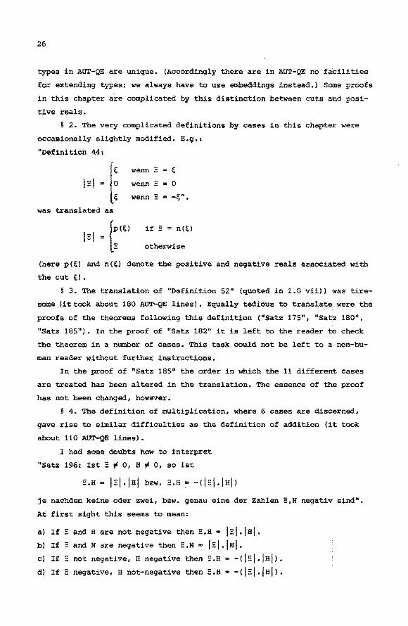
§ 2. The very complicated definitions by cases in this chapter were
occasionally slightly modified. E.g.:
"Definition 44:
1•1 - {; wenn - ~
wenn E :: 0
wenn - -~".
was translated as
{•<tl if E = n(~)
1=1 = otherwise
(here p(~) and n(~) denote the positive and negative reals associated with
the cut~).
§ 3. The translation of "Definition 52" (quoted in 1.0 vii)) was tire
some (it took about 180 AUT-QE lines). Equally tedious to translate were the
proofs of the theorems following this definition ("Satz 175", "Satz 180".
"Satz 185"). In the proof of "Satz 182" it is left to the reader to check
the theorem in a number of cases. This task could not be left to a non-hu
man reader without further instructions.
In the proof of "Satz 185" the order in which the 11 different cases
are treated has been altered in the translation. The essence of the proof
has not been changed, however.
§ 4. The definition of multiplication, where 6 cases are discerned,
gave rise to similar difficulties as the definition of addition (it took
about 110 AUT-QE lines).
I had some doubts how to interpret
"Satz 196: Ist E 'I 0, H 'I 0, so ist
je nachdem keine oder zwei, bzw. qenau eine der Zahlen E,H negativ sind".
At first sight this seems to mean:
a) If - and H are not negative then E,H = 1=1-lal. b) If - and B are negative then E.B = 1=1-lal. c) If - not negative, H negative then E.B -<IEI.Ial>. d) If E negative, H not-negative then E.B = -<1=1-lal>·

27
However, if this meaning is intended the condition E ~ 0, B ~ 0 is super
fluous. Therefor~, possibly, the statement is meant to include also
e) If E.B
f) If E,H
IEI.Ial then neither or both of E and Hare negative.
-<IEI.!al> then E is negative and His not, or His negative
and E is not.
Landau's proof ("Beweis: Definition 55") does not give a clue, and in later
references to the theorem he only uses a), b), c) or d). Nevertheless I have
formalized proofs of e) and f) in the translation.
"Satz 194" and "Satz 199" have complicated proofs by cases, which were
not easy to formalize.
§ 5. The "Vorbemerkung" to "Satz 205" requires two proofs. Some lemmas
are needed for the proof of the "Hauptsatz" itself, e.g. it is used that 1 B E. H = E (cf. 2.4). No special difficulties arose in proving this important
theorem.
2.6. The alternative version of chapter 4
Our motivation to write another version of chapter 4, called chapter 4a,
was discussed in 2.1 x). In this chapter the theorems of chapter 4 are
proved for reals which are defined in a way different from Landau' s. Also
the order in which these theorems appear differs from Landau's order.
At the .end of this chapter the square root of a nonnegative real is
defined using "Satz 161", and its prope:r::ties are derived. (This has been
done by Landau·in "Kapitel 5, § 7"),
The lengthS of the AUT-QE texts of chapter 4 and chapter 4a are about
equal.
2.7. The translation of "Kapitel 5"
The actual translation of this chapter is preceded by a number of lem
mas. Some of these give properties of division on the reals, implicitly
used by Landau in the sequel. Further there are lemmas describing the shift
of a segment of integers y,y+l,y+2, ••• ,x to an initial segment of the natu
rale 1,2, ••• ,(x+1) -y, which serve the translation of§ 8.
The translation of the first seven paragraphs of this chapter was
straightforward. Preceding the proof of "Satz 221" some lemmas .appear, des
cribing, for a complex number x, the properties of Re(x) 2 + Im(x) 2• These
properties are used by Landau without notice in the proofs of "Satz 221"
28
and "Satz 229" and in the definition of lxl ("Definition 66"). (In my opi
nion, at least a remark should have been made in this definition, to the ef-2' 2
feet that Re(x) + Im(x) ~ 0 for complex x),
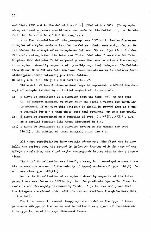
§ 8. The translation of this paragraph was difficult. Landau discusses
x-tuples of complex numbers in order to define their sums and products. He
introduces the concept of an x-tuple as follows: "Es sei f(n) fQr n ::> x de
finiert", and explains this later on: "Unter "definiert~· verstehe ich "als
komplexe Zahl definiert". After proving some theorems he extends the concept
to x-tuples indexed by segments of (possibly negative) integers: "In Defini
tion 70 und Satz 284 bis Satz 286 bezeichnen ausnahmsweise lateinische Buch
stabeng?Ilze (nicht notwendig positive) Zahlen.
Es sei y :5: x, f(n) fQr y ::> n :> x definiert .. , ....
There are (at least) three natural ways to represent in AUT-QE the con
cept of x-tuple indexed by an initial segment of the naturals:
i) f might be considered as a function from the type nat to the type
ex of complex numbers, of which only the first x values are taken in
to account. If we take this attitude it should be proved that if f and
g coincide for n ::> x then their sums (and products) up to x are equal.
ii) f might be represented as a function of type [t,nat][U,t::>X]CX , i.e.
as a partial function like those discussed in 1.4.
iii) f might be considered as a function having as its domain the type
lto(x) , the subtype of those naturals which are ::> x.
All these possibilities have certain advantages. The first one is pro
bably the easiest one, the second is in better harmony with the rest of our
AUT-QE translation, the third maybe corresponds better with Landau's inten
tions.
The third formalization was finally chosen, but caused quite some trou
ble because (on account of the unicity of types) numbers of type lto{x) do
not have also type lto{x+l) • As to the formalization of x-tuples indexed by segments of the inte
gers, there was the extra difficulty that the predicate "ganze Zahl" on the
reals is not thoroughly discussed by Landau. E.g. he does not prove that
the integers are closed under addition and subtraction, though he uses this
in the text.
For this reason it seemed inappropriate to define the type of inte
gers as a subtype of the reals, and to define f as a (partial) funption on
this type in one of the ways discussed above.

29
Therefore we defined f, for fixed integers x and y, as a function of
type [t,real][u,int(t)J[u,y~tsx]cx , i.e. as a partial function on the
reals. (rather like [t.nat][u.tsx]cx. , see ii) above).
With this formalization of x-tuples (resp. (x+l)-y-tuples) the trans
lation of § 8 turned out to be laborious. Many rather meaningless embedding
and lifting functions appear in the proofs. In particular the proof of
"Satz 283" where it is shown that sums (products) are invariant under per
mutations of their terms (factors) turned out to be long and tedious. (It
should be remarked that Landau's proof is long too: 4 pages, 87 lines of
German text, while the translation needs 365 .lines of AUT-QE text.)
The last two paragraphs did not present difficulties in translating.

30
3. VERIFICATION
In this chapter the verification of the AUT-QE text is described. Some
features of the program and the possibility of excerpting are discussed.
3.0. Verification of the text
The verification of the AUT-QE translation of Landau's book was execut
ed on the Burroughs B6700 computer at the Technological University of Eind
hoven. The last page of the book was checked in September 1975. The whole
book was checked in a final run on October 18, 1975. The verifying program
was conceived by N.G. de Bruijn and implemented by I. zandleven. For a des
cription of this program we refer to [Zl]. Zandleven also provided the pro
gram with input and output facilities, and extended it with a conversatio
nal mode for on-iine checking and correcting of texts.
The verification took place in three stages:
i) First the AUT-QE text was fed into the system on a teleprinter. At
this stage the main syntactical structure of the text was analyzed. It
was checked, for example, that the format of the lines was as it should
be, that the bracketing of the expressions was correct, and that no un
known identifiers occurred.
ii) Secondly the AUT-QE text was coded. At this stage the correct use of
the context structure, the validity of variables, the correct use of
the shorthand faoiZity [vD, 2.15] and of the paragraph reference sys
tem (cf. appendix 2), were checked.
iii) Finally the text was checked with respect to all clauses of the langua
ge definition. At this stage the degveee [vo, 2.3] and types of expres
sions were calculated, and the correctness of application expressions
and constant expressions was checked. Vital for this is the verifica
tion of the definitional equality of certain types (cf. [vD, 2.10],
[Zl]) •
Runs of the stages ii) and iii) generally claimed much of the compu
ters (virtual) memory capacity (over 600K bytes was needed for the program
together with the coded text). In order to avoid congestion in the multi
programming system it was therefore necessary to have the program executed
at night (and off-line). As AUTOMATH texts are checked relative to correct books,
a mechanical provisional debugging device for off-line checking was implemen
ted, by which lines which were found incorrect could be tentatively repaired.

31
E.g. , when the mi&:J:te pal't [ vD, 2 • 13 • 1] of a line was found incorrect, the
debugging device changed it temporarily into PN, thus turning an abbrevia
tion line into a PN-line. 'l'he line so "corrected" was then again checked,
and, if it was found correct, the lines following could then be checked relative to
the "corrected" book. By this device it was not necessary to stop the check
ing immediately after the first error had been found.
Another feature of the verifying program was added because of the fact
that proving expressions to be incorrect (especially proving expressions to
be not definitionally equal) is often more difficult and more time-consum~
ing then proving correctness. Therefore during off-line runs a parameter in
the program (viz. the number of decision points, to be explained in 3.1) has
been limited, and lines were considered provisionally incorrect when this
limit was exceeded.
When the later chapters were checked, we reduced the demands on the
computers memory capacity by abridging the book relative to which the text
was checked, in the following way: In the chapters which had already been
found correct, the proofs of theorems and lemmas were omitted, and the final
lines of these proofs (where the theorems and lemmas are asserted) were
changed into PN-lines. Each time a chapter was completely checked (relative
to the book so abridged) it was abridged in its turn.
Text which are correct relative to the abridged book will be correct
with respect to the unabridged book too. On the other hand, as in classical
mathematics there is no reference to proofs but only to assertions, it is
unlikely that texts which are correct relative to the unabridged book will
be rejected relative to the abridged book. In actuai fact this did not
occur.
When a chapter, after several off-line runs of the program,wasfound
to be "nearly correct", the final verification of that chapter took place
on-line. In such an on-line run the remaining errors could be immediately
corrected. Moreover correct lines could be verified, which had been provi
sionally rejected because the nUmber of decision points during verification
in off-line runs had exceeded the chosen limit. The verification of such
complicated lines could be shortened by directing (in conversational mode)
the strategy for establishing definitional equality.
After all chapters were verified in this way, the integral AUT-QE
text (complete and unabridged) was checked during a final on-line run,
which took 2 hours (real time). Of this time 42 min was spent on verifica
tion (not including the time needed for coding).

32
In a table we list some data on this final run, concerning ver.ification
time, number of performed reductions and memory occupied
preliminary chapter chapter chapter chapter chapter chapter complete
text I 2 3 4a 5 4 text
verification time 107.3 143.1 301.2 342.4 405.7 813.1 406.9 2519.7
in seconds
a-reductior's 63! 752 1077 1455 1644 3393 1533 10485
a-reductions 564 832 460 466 414 2749 529 6014
IS-reductions 596 !Ill 1318 1873 2724 9290 3151 20063
n-reductions 2 - - - - - - 2
nr. of lines 1068 886 1603 2181 2779 2690 2226 13433
nr. of expressions 9388 12155 25792 30327 42067 60450 34959 215138
Since one coded expression occupies about 30 bytes (mainly used for referen
ces to subexpressions) , the total memory required for the coded book is
about 6500 K bytes <~ 52000 K bits).
3 .1. Controlling the strategy of the program
In order to establish definitional equality of two expressions, the
verification system tries to find another expression to which both reduce.
The choice of efficient reduction steps for this purpose is a matter of
strategy ([vD, 6.4.1]). The programmed strategy is described in [Zl].
Under this strategy it is possible that intermediate results are ob
tained which strongly suggest a negative answer to the question of defini
tional equality, without definitely settling it. Suppose, for example, that
a(p)=a(q) has to be established. The programs strategy is to ascertain
that the constants a and a are identical and to verify whether p=q If this is not the case, there is a strong suggestion that a(p) and a(q) are not definitionally equal either, but this is yet uncertain. For example,
they are definitionally equal relative to the book
* n .- PN f type
* p .- PN E n
* q .- PN E n
* X .- E n
X * a .- p E n
It is a matter of strategy how to proceed in such cases. we may either
apply a-reduction (in which case the issue will be eventually settled) or
we may try to continue the verification process without using a(p)=a(q) .

33
such a situation is called a decision point. In on-line runs the veri
fication may be controlled here by the human operator. (Actually, in the
situation sketched above, information will be supplied, and the question
will appear whether o-reduction should be tried.) In off-line runs o-reduc
tion will be applied in order to get a definite answer to the question, and
it will be checked that the total number of decision points passed during
the checking of a line does not exceed the chosen limit (cf. 3,0).
3.2. Shortcomings in the verifying program
In appendix 5, two shortcomings in the verifying program are indicated,
Due to these shortcomings there is, at this moment no complete (mechanical
ly sustained) certainty that the verified AUT-QE text is correct.
It is hard to believe, however, that any incorrect AUT-QE lines have
been accepted by the machine during verification. We mention the following
rather intuitive considerations in support of this opinion:
i) Given a correct AUT-QE expression, we can consider all possible ways to
change it into an incorrect one by replacing, somewhere, a bound varia
ble by an other one. Only a very small fraction of these possibilities
will give rise to incorrect expressions which the program (unjustly) accepts. For most expressions this fraction will even be 0. As the writer
intended to produce correct AUT-QE expressions, and as he did not make
many mistakes using wrong variables, it is improbable that incorrect ex
pressions have been accepted,
ii) No correct expressions have ever been refused during the verification,
though the number of correct expressions presented exceeded considera
bly the number of incorrect ones.
Before long the text will be verified by an entirely new program, in
which clash of variables is impossible because the coding system uses name
teas variables ([dB2]).
3.3. Excerpting
Let B be an AUT-QE book, i.e. a finite sequence of lines. A eubbook of
B is a subsequence of this sequence. A program, called excerpt, is availa
ble which, given a correct book B and a line ! of B, produces the minimal
correct subbook of B containing £. (It is possible to have the line provi
sionally changed into a PN-line before the subbook is produced.)
34
This program will display all concepts relevant to the definition of a
given concept, a~d all theorems (with their proofs) used (explicitly or im
plicitly) in the proof of a given theorem. (If the line is first chanqed in
to a PN-line, the program will just give the assumptions under which the
theorem holds, and the concepts necessary to understand its contents,)
As an example, we give in appendix 4 an excerpted text for "Satz 27".

35
4. CONCLUSIONS
In this chapter we discuss some possibilities to represent logic in
AUTOMATH, we indicate some desirable extensions of AUT-68 and AUT-QE, and
we discuss some aspects (positive as well as negative) of our translation,
4.0. Formalization of logic in AUTOMATH
In this section \fa shall describe various possibilities to represent
systems of natural deduction in AUT-68 ((vo, 2]), in AUT-QE and in some
closely related languages. First we discuss two main decisions which have
to be made when choosing between these possibilities. Then we indicate ex
plicitly two possibilities to represent logic.
4.0.0. First orderv. higher order
In most AUTOMATH languages there are certain restrictions on abstrac
tion. E.g. in AUT-68 as well as in AUT-QE correct abstraction expressions
have the form [x,a]A where a is a 2-expression (and hence x, having type a,
is a 3-variable, i.e. a variable which is a 3-expression).
Such restrictions allow a faithful representation of first order logic
(in the sense of excluding higher order formulas and inferences). In AUT-68
as well as in AUT-QE this can be done by representing propositions and pre
dicates as 2-expressions (as described in (vo, 3]). Then proposition varia
bles and (in AUT-QE) predicate variables will be 2-variables and abstrac
tion (or quantification) with respect to such variables is impossible in
the language. If, in such a setting, we want to discern between proposition
variables and predicate variables then it is necessary to have abstraction
expressions of degree 1 in the language, i.e. to use AUT-QE (and not
AUT-68).
In order to represent higher order logic we should require the possi
bility of abstraction with respect to proposition and predicate variables.
Therefore, if we stick to the abstraction restrictions of AUT-68 or AUT-QE,
we should represent propositions and predicates by 3-expressions. We may
proceed in two ways:
i) we can associate to each proposition a (primitive) type (which we will
call the assePtion type of the proposition). Objects of this type will
be considered as proofs of the proposition. In other words: we consider
the proposition as asserted iff its assertion type contains some object.
This possibility will be elaborated in 4.0.2.
36
ii) we can extend the language to a new language, called AUT-4, by admitting
4-exp~eesions (having 3-expressions as their types (cf. [vD, 2.3]). Then
a proposition (represented by a 3-expression) might be considered as as
serted if it contains something (some 4-expression). Thus propositions
act as their own assertion types, and the representation of logic is
just as described in [vD, 3.2], but for a shift with respect to degrees.
4.0.1. Relevance of proofs vs. irrelevance of prOofs
In all representations of logic in AUTOMATS languages which have been
developed so far, proofs (i.e. names of proofs) appear in the language
([vD, 3], [dB], [dV]). In this respect these representations reflect a con
structive conception of logic, in which proofs and objects are treated simi
larly.
In a classical conception of logic, proofs are discussed in the meta
language only. As a consequence it is impossible in such a conception to
discern (in the language) between different proofs of one proposition. This
point of view can be roughly represented in AUTOMATS by proclaiming, for any given
p;0positi0n a 1 aJ.l prOOfS Of a tO be equal, ThiS depriVeS these proofS
of their identity, their names should be considered only as references to
the place in the book where the proposition is asserted. This possibility
has been first suggested by de Bruijn.
If, in a representation of logic in AUTOMATH, such an attitude is adop
ted, we shall say that this representation satisfies i~~ezevance of p~ofs.
(Cf. [Z], and also 1.4). How this irrelevance of proofs is implemented
(i.e. in which sense proofs are considered "equal") will depend both on the
language and on the way logic is represented in it (cf. 4.0.3 i) and ii)).
4.0.2. A representation of logic in AUT-68
A higher order system of natural deduction can be formalized in AUT-68
as follows.
A type of propositions is introduced as a primitive type:
* PROP : = PN I ~ and to each proposition A its assertion type r{A) is associated:
* A .A * r .- PN
E PROP
I~

37
(In earlier publication on AUT-68, bool and TRUE were used instead of
PROP and 1- ) • I.f S is a type, an object P f [X ,SJPROP has to be inter
preted as a predicate. Objects of type [x,SJr(<X>P) must then be inter
preted as proving that P holds for every X f S • So we want to introduce
the proposition V(S,P) which has the property that its assertion type con
tains elements iff the type [X,SJI-{<X>P) contains elements. This is ex-
pressed in the following
* s .-s * p := p * V .-p * a := a * u .-u *Ve .-p * u := u *Vi .-
lines:
PN
PN
PN
fill! f [x,SJPROP
E PROP
E S
f 1-(v(S,P))
f H<a>P)
f [x,SJI-(<x>P)
E 1-(v(S,P))
Starting from these primitive concepts and axioms, higher order logic can
be developed. An indication of how this can be done, is given in appendix 6,
where the first three theorems from Landau's book are derived on the basis
of the logic so developed.
This logic represents a constructive system of natural deduction.
Axioms could be added for extensional equality of functions and extensionaZ
equaZity of propositions (i.e. if a++ b then a= b).
Classical logic could be represented this way by adding axioms for ir
relevance of proofs:
*A .- E PROP
A * u .- E 1-(A)
u * V .- E 1-(A)
V * irr.pr ... .- PN f IS(I-(A),u,v)
and for the double negation law:
A * u .- E H•(•(A)))
u * d.n.l. .- PN E 1-(A)

38
4.0.3. A representation of logic in AUT-QE
How logic can be represented in AUT-QE is described in [vD, 3]. This
system, a first order system of natural deduction, has been used in our
translation. An indication of the development of logic in it can be found
in the excerpted text in appendix 7, which covers the proofs of the first
three theorems of Landau' s book and the logic used in these proofs.
The system is a bit ambivalent, because it is classical {containing the
double negation law as an axiom) but does not satisfy irrelevance of proofs.
There are two obvious ways to implement irrelevance of proofs:
i) by adding an axiom:
* A .- I~ A * s .- I~ s * t := I [x,AJS t * u .- E A
u * V .- EA
V * irr.pr. .- PN I IS(S,<u>t,<v>t)
That is: if to every proof of A an object of type S is associated,
then this object is independent of the nature of the proof. It has been
indicated by J. zucker that this axiom implies irrelevance of proofs in
partial functions as mentioned in 1.4:
* s s * T
T * p p * f
f * a a * b
b * u
u * V
V * w
.-
.-·-.-.-:=
:= .-.-.-
I~ I~ I [x,SJ~ I [x,SJ[y,<x>PJT
E S
E S
I IS(S,a,b}
E <a>P
E <b>P
w * Q .- [x,SJ[y,<x>PJIS(T,<u><a>f,<y><x>f) I [x,SJ~ W*il .- [y,<a>PJirr.pr.(<a>P,T,<a>f,u,y) I <a>Q
w * t 2 .- ISP(S,Q,a,b,u,t1) I <b~Q
w * t 3 .- <w>t2 I IS(T ,<u><a>f ,<w><b>f)

39
ii) by extending, in the language, the relation of definitional equality,
in such a way that two 3p-expressions (cf. 1.2) are definitionally equal
iff their types are definitionally equal. This has been done in the lan
guage AOT-TI (cf. [Z]), but could be done in a variant of AUT-QE as well.
If we want to formalize intuitionistic logic in AUT-QE we should have
the absurdity rule (i.e. contradiction implies any propos~tion) instead of
the double negation law. The logical connectives (apart from implication)
and the existential quantifier could be added as primitive constants, and
their elimination- and introduction rules as axioms.
4.1. The language
In this section we discuss some features of AUTOMATH languages, and
the value of these features for the formalization of mathematics.
4.1.0. AUT-SYNT
Consider the following AUT-QE text, representing the introduction rule
for conjunction:
* a a * b
b * u
u * V
V * andi
.-
.-:= .-.-
f~ f~ E a E b ~ and(a,b)
(where the dots indicate some proof which is irrelevant for the present dis
cussion). We will call the variables a,b,u,v the parameters of andi • If we
want to apply this rule for propositions A and B, we need two proofs p and q
of the propositions, thus getting the proof andi(A,B,p,q) ~ and(A,B).
Suppose we are given the proof p, then we can compute mechanically its
type (Cf., [vD, 6.4.2.3]) which is (definitionally equal to) the proposition
A it proves. A similar observation holds for q and B. Hence we could say
that the expression andi(A,B,p,q) contains redundant information. If the
"mechan.ical type" function CAT ([vn, 6.4.2.3]) were incorporated in the lan
guage, we could write, instead of the expression above, andi(CAT(p),CAT(q),
p,q),·which only contains p and q. We will call the parameters U and V
(for which p and q are substituted) the essential parameters of andi , while a and b (for which the redundant expressions A and B are substituted)

40
are called Pedundant parametePe. There are many other examples of expres
sions with redundant parameters.
It is worth while to extend the language in such a way that redundant
parameters can be avoided, because the expressions which have to be substi
tuted for them might be long. A system of extensions of this kind has been
proposed by I. Zandleven. It is called AUT-SYNT since it.admits syntactic
vaPiabtee for expressions. Thus we have the languages AUT-68-SYNT, ·AUT-QE
SYNT etc.
For a description of AUT-SYNT we refer to appendix 9, a text in AUT-
68-SYNT may be found in appendix 8.
OUr experiences with translating Landau's book have been a stimulus
for developing AUT-SYNT, and have indicated the way this could be done. As
no verifying program for SYNT languages was available until after the trans
lation was finished, the SYNT-facility could not be used in the translation.
This may be considered unfortunate, because the presence of this facility
would have simplified both the writing and the reading of our text.
4.1.1. n-reduction in AUTOMATH
In AUT-68 and AUT-QE one of the possible ways to establish definitional
equality is by n-reduction ([vD, 6.2.2]): If xis not free in A then
[x,a]<x>A >n A. As can be seen in the list in 3, n reduction was applied
only twice during the verification of our translation. We give the lines
which required these n-reductions, together with their relevant contexts.
The following lines from the text on prepositional logic are presup
posed:
* con .- PN I .~?.!:!?.E. * a .- I .~?.!:!?.E.
a * not .- cx.a]con I .~?.!:!?.E. a * u .- f not(not{a)) u * et := PN E a a * u := E con u * cone := et(a,[x,not(a}Ju} fa
The first line where n-reduction is required occurs in the text on pre
dicate logic. In this text the following lines appear:

41
* s ·- ~~ .-s * p := ~ [X,S)~
P * all .- p ~~ P * non := [x,SJnot(<x>P) ~ [X,S]~ p * u := ~not( all (S,P)) U * V .- ~ non(non(P))
V * s := E S
s * tl .- et( <s>P ,<s>v) E <s>P
V * t2 := <[x,SJtl(x)>u E con
In order to verify that the middle part of this last line is a correct ex
pression, it should be established that
we have
CAT([x,SJtl(x)) ~ DOM{u) (Cf; [vD, 6.2.4.6]) •
CAT([x,S]tl(x)) = [x,SJCAT(tl(x)) = [x,SJ[s/x]<s>P = [x,S]<X>P ,
DOM(u) = DOM{not(all{S,P))) = DOM([x,all(S,P)Jcon) = all(S,P) ~p
The question is to establish
[X,S]<X>P Q P •
This obviously requires n-reduction.
The second case in which n-reduction is used occurs in the text on ge
neralized implication:
* a .- ~~ a * b ·- ~ [x,aJ~ .-b * imp .- b ~~ b * u .- f not(a)
u * th2 .- [x,a)cone{<x>b,<x>u) ~ imp{a,b)
Here, in order to verify the last line, it is asked whether the category of
the middle part definitionally equals the category part, i.e. whether
Now
CAT([x,a]cone(<x>b,<x>y) ~ imp(a,b) •
CAT([x,aJcone(<x>b,<x>u)) = [x,aJCAT(cone{<x>b,<x>u)) =[x.aJ<x>b ,
imp(a,b) Q b
and therefore n-reduction must be used for establishing
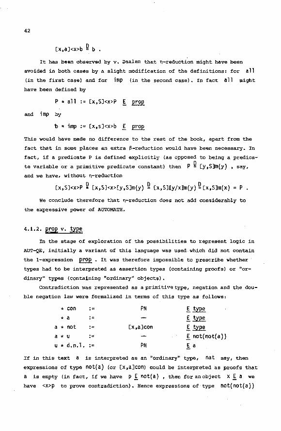
42
D [x.aJ<x>b = b •
It has been observed by v. Daalen that n-reduction might have been
avoided in both cases by a slight modification of the definitions: for all
(in the first case) and for imp (in the second case), In fact all might
have been defined by
P * all := [x,SJ<x>P E ~
and imp by
'b * imp .- [x,sJ<x>b f ~
This would have made no difference to the rest of the book, apart from the
fact that in some places an extra S-reduction would have been necessary. In
fact, if a predicate P is defined explicitly (as opposed to being a predica
te variable or a primitive predicate constant) then P Q [y,SJm{y) • say,
and we have, without n-reduction
[x,SJ<x>P ~ [.x,S]<X>[y,SJm{y) ~ [x,SJ[y/x)m(y) ~ [x 1 S]m(x) = P •
we conclude therefore that n-reduction does not add considerably to
the expressive power of AUTOMATH.
4.1.2. ~ v. ~
In the stage of exploration of the possibilities to represent logic in
AUT-QE, initially a variant of this language was used which did not contain
the 1-expression ~ • It was therefore impossible to prescribe whether
types had to be interpreted as assertion types (containing proofs) or "or
dinary" types (containing "ordinary'' objects).
Contradiction was represented as a primitive type, negation and the dou
ble negation law were formalized in terms of this type as follows:
* con .- PN f~ * a .- f~
a * not .- [x,aJcon f~ a * u := f not(not(a)) u * d.n.l. .- PN E a
If in this text a is interpreted as an "ordinary" type, nat say, then
expressions of type not( a) (or [X 1a]con) could be interpreted as proofs that
a is empty (in fact, if we have p f not{ a) , then for an object X E a we
have <X>p to prove contradiction). Hence expressions of type not(not(a))

43
have to be interpreted as proofs that a is (in a weak sense) nonempty.
Given such a proof q we have an object d.n.l(a.q) I a. Or, in other
words: d.n.l actsas a Hilbert operator, selecting an object from any non
empty type. In particular this induces a form of the axiom of choice.
As we did not want the double negation law to have such far-reaching
consequences, we extended the language by admitting ~ as a basic 1-
expression. Thus we obtained the language AUT-QE (as defined in [vD, 5]),
in which it is possible to distinguish between assertion types and ordinary
types.
The distinction of ~ and ~ not only unlinked the double negation
law from the axiom of choice, but also made it possible to implement irrele
vance of proofs (cf. 4.0.1, 1.4). This opportunity was not seized in the lo
gic underlying our translation (though this would have been natural). For
an explanation we refer to 4.2.1.
We may conclude that the distinction between proofs and "ordinary" ob
jects is an essential feature when representing classical logic in AUTOMATH.
For representing constructive logic the version with only ~ keeps its
value.
4.1.3. Strings and telescopes
In chapter 2 of his book Landau uses pairs (x1,x2) .of natural numbers.
He considers such a pair as a single object and yet he describes it by two
variables. A faitp£ul translation of this practice could have been given if
the concept of a at~ing of erepreasiona would have been present in our lan
guage.
Another use strings of expressions might have is as arguments of par
tial functions {as described in 1.4). In fact such functions are applied to
pairs (a,p) where a is an object of a certain type S , and p a proof
that a satisfies some predicate P on S (which describes the range of
the function) •
As a further example we consider the concept of a group, which might
be considered as a string (S,op,iv,e,p) where S I~• op I [x,S][y,S]S, iv I [x,SJS, e IS and pI groupaxioms(S,op,iv,e) •
We usually want the types of the expressions of such a string to satis
fy certain conditions. In the case of the argument (a,p) of partial func
tion we want a I S, p I <a>P • In other words we want the argument (a,p) to be consistent with the "abstractor part" of the function: X I S
y I <X>P • In the case of the group we want a group (S,op,iv,e,p) to be

44
consistent with
x f~; y f [s,xJ[t,xJx; z f [s,xJx; u f x;
v f groupaxioms(x,y,z,u)
There is a strong analogy with the case where expressions A1, ••• ,An are re
quired to be suitable candidates for substitution for the variablesx1
, •• ,xn
of a certain context x1 E a 1,x2 E a 2 , ••• ,x Ea (Cf. [vD, 2.5]). . - - n- n
To describe such conditions on strings we introduce the following ter-
minology. f' finite sequence of ! formulas x1 ! a 1 , ••• ,xn ! an is called a
telesaope. The string of expressions (a1, ••• ,an) is said to fit into the
telescope x1 ! a 1 , ... ,xn! an if a 1 ! a1 ,a2 ! fxla1 Ja2 , ... ,
a E lx1
, ••• ,x 1!a
1, ••• ,a
1]a • n- n- n- n
Extension of the language with constants and variables for strings
and defined constants for telescopes has been proposed by de Bruijn. This is
especially helpful, when formalizing abstract structures such as groups,
vect~r spaces or categories, and has been applied on a large scale by
J. zucker (Cf. [z]).
4.2. Comments on the translation
In this section we first give a chronological survey of the different
representations of logic which have been tried, and we state the motives
for finally choosing AOT-QE as a language for our translation. Furthermore
we mention some aspects which are (in our opinion) shortcomings of the
translation and we add some positive conditions which can be drawn from our
work.
4.2.0. Choice of the language
In our first attempts to translate Landau's "Grundlagen" in AOTOMATH,
we used the language AOT-68. The representation of logic was similar to the
one described in 4.0.2 and presented in appendix 6. Elimination and intro
duction of V were effected by the axioms Ve (with parameters S f ~· p f [x,SJPROP, a f S, u f r(V(S,P)) J and Vi (with parameters S f~• P f [x,S]PROP, u f [X,S]r(<x>P) ) • These axioms were used frequently in de
veloping logic, because the logical connectives and the existential quanti
fier were defined in terms of V • On the basis of this logic chapter 1 of
Landau's book was translated in AUT-68.
45
At that stage of our work we started trying to represent logic in
that language which did not contain AUT-QE, initially using a variant of
~· In AUT-QE the axioms Vi and
(i.e. P represents a predicate on
Ve were superfluous: if P I [x.SJ~ S J then objects of type P can be
inte~preted as proofs of V(S,P) • Conversely, given such an object u I P and an object a E S we have <a>u I <a>P (i.e. <a>u proves that P holds at a). As a consequence the text on logic in AUT-QE was considera
bly shorter then the earlier text in AUT-68. (It was not observed at that
time, that this was caused essentially by the redundant parameters S and
P of both constants Ve and Vi ,) so AUT-QE seemed to be a much better
language, and therefore a fresh start was made with the translation of
Landau's book into .that language. In 4.1.2 we have reported that in this
system (AUT-QE without ~ the double negation law induces a Hilbert ope
rator. This led us to add ~as a basic 1-expression to our language, thus
extending it to proper AUT-QE.
At the time we finally fixed the language we did not appreciate the
fundamental importance of incorporating a form of irrelevance of proofs.
This was due mainly to two reasons:
i) Partial functions are not frequently used in the first three chapters
of Landau's book, and for those partial functions which are defined
there, irrelevance ofproofscould be derived. Therefore no need was
felt for an axiom.
ii) As Landau, being a classical mathematician, does not discuss proofs at
all, we thought we should try to follow this practice. Consequently we
did not want to have an axiom declaring proofs equal.
4.2.1. Shortcomings of the translation
Here I list those features of the translation which I weuld change if
I were to redo the work.
i) In my opinion the SYNT-facility should be present in any AUTOMATH lan
guage. It will bring texts in AUTOMATH closer to mathematical practice.
The middle parts of many lines in the present Landau translation are
unnecessarily complex and tedious (both to the reader and to the wri
ter), because this facility is absent in the language I used.
ii) I regret that I have not implemented irrelevance of proofs as an axiom.
As I see it now, for representing classical reasoning a language should
be chosen which even contains irrelevance of proofs by definitional
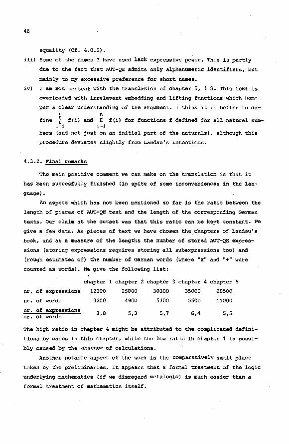
46
equality (Cf. 4.0.2).
iii) some of the names I have used lack expressive power. This is partly
due to the fact that AUT-QE admits only alphanumeric identi~iers, but
mainly to my excessive preference for short names.
iv) I am not content with the translation of chapter 5, § 8. This text is
overloaded with irrelevant embedding and lifting functions which ham
per a clear understanding of the argument. I think it is better to de-n n
fine L f(i) and n f(i) for functions f defined for all natural num-i=l i•l
bers (and not just on an initial part of the naturals), although this
procedure deviates slightly from Landau's intentions.
4.3.2. Final remarks
The main positive comment we can make on the translation is that it
has been succesfully finished (in spite of some inconveniences in the lan
guage).
An aspect which has not been mentioned so far is the ratio between the
length of pieces of AUT-QE text and the length of the corresponding German
texts. Our claim at the outset was that this ratio can be kept constant. We
give a few data. As pieces of text we have chosen the chapters of Landau's
book, and as a measure of the lengths the number of stored AUT-QE expres
sions (storing expressions requires storing all subexpressions too) and
(rough estimates of) the number of German words {where "x" and "+" were
counted as words). We give the following list:
chapter 1 chapter 2 chapter 3 chapter 4 chapter 5
nr. of expressions 12200 25800 30300 35000 60500
nr. of words
nr. of expressions nr. of words
3200
3,8
4900
5,3
5300 5500 11000
5,7 6,4 5,5
The high ratio in chapter 4 might be attributed to the complicated defini
tions by cases in this chapter, while the low ratio in chapter 1 is possi
bly caused by the absence of calculations.
Another notable aspect of the work is the comparatively small place
taken by the preliminaries. It appears that a formal treatment of the logic
underlying mathematics (if we disregard metalogic) is much easier than a
formal treatment of mathematics itself.

47
It has not been the purpose of this enterprise to construct a formal
system which suits my own fancy and to develop in this system the theory of
naturale, reals and complex numbers. I have rather tried to represent in a
language which was essentially given beforehand, a wide variety of concepts
and ideas as expressed in a book like Landau's. The success of this under
taking is due to the flexibility of AUTOMATH languages, and to the close
connection which can be made between these languages and intuitive human
reasoning.
48
Appendix 1. REPRINT. Published in the
Proceed~ngs of the Symposium
on APL (Paris, December 1973),
ed. P. Braffort.
A description of AUTOMATH and some aspects of
0. Summary
its language theory
by
*) D.T. van Daalen
This note presents a self-contained introduction into AUTOMATE, a formal
definition and an overview of the language theory. Thus it can serve as an
introduction to the papers of L.S. Jutting [7] and I. Zandleven [11] in this
volume. Among the various AUTOMATH languages this paper concentrates on the
original version AUT-68 (because of its relative simplicity) and one eXten
sion AUT-QE (in which most texts have been written thus far).
The contents are:
1. Introductory remarks.
2. Informal description of AUT-68.
3. Mathematics in ATJ'I'CMATH: propositions and types.
4. Extension of AUT-68 to AUT-QE.
5. A formal definition of AUT-QE.
6. Some remarks on language theory.
For a description of the AUTOMATH project and for its motivation we refer
to Prof. De Bruijn's paper also in this volume [4].
*) The author is employed in the AUTOMATE project and is supported by the
Netherlands Organization for the Advancement of Pure Science (Z.W.O).

49
1. Introductory remarks
1.1. According to the claims for the formal system AUTOMATH one should be
able to formalize many mathematical fields in it in such a precise and com
plete fashion that machine verification becomes possible. The flexibility
required to meet the indicated universality is provided by having a rather
meagre basic system. The AUTOMATH user himself has to add appropriate primi
tive notions to the ba=ic system in order to introduce the concepts and
axioms specific to the part of mathematics he likes to consider. In this
respect, the basic system may be compared with some usual system of logic
(e.g. first order predicate calculus) to which one adds mathematical axioms
in order to form mathematical theories.
1.2. In spite of this analogy however the basic system itself does not con
tain any logic in the usual sense. Basic for the system are the concept of
type and function (instead of, e.g., the concept of set or of natural num
ber), which are formalized by a certain typed A-caZcuZus.
When representing mathematics in AUTOMATH one has to deal with the
question of coding: How to formalize general mathematical concepts in the
form of types and functions (see section 2.2). Clearly an appropriate
formalization will incorporate as much as possible of the basic type-and
function framework. Section 3 discusses this coding problem and in particu
lar proposes a suitable way of representing propositions, predicates and
proofs (a functional interpretation of logic).
1.3. In order to satisfy the claim of automatic verification of correctness
the system certainly has to be decidable (and even feasibly decidabZe on now
existing computing machines). Since many common mathematical theories pro
duce undecidable sets of theorems we must conclude that we cannot expect
the computer to do all our work. Indeed theorems have to be given together
with their proofs in order to allow verification.
Thus the correctness produced by the machine verification covers the
arguments leading from axioms to conclusions only. The AUTOMATH user him
self is responsible for his choice of primitive notions and all the coding
(and decoding) involved.

50
2. Informal description of AOTOMATB
2 .1. Introduction
Here we treat the original version of AUTOMATB, now named AUT-68. We
chose this system as an example because of its relative simplicity. The
discussion will be informal and intuitive and in fact restricted to the
object-and-type fragment of the language (thus leaving the proof-and-pro
position fragment to section 3).
2.2. Intuitive framework
(This section may be skipped by formalists).
The mathematical entities discussed in the language fall into two sorts:
objeats and types. The types may be considered as classes or sets of a cer
tain kind, which may have objects as their elements. All types are supposed
to be disjoint, for each object belongs to just one type. This uniqueness
of types permits one to speak about the type of an object.
The typestructure is built up by starting from gPound types and forming
~motion types from these. Each mathematician may choose the ground types
himself (as primitive notions), e.g. the type of natural numbers.
An example of a function type is the type a + ~ (where a and ~ are
types) of the functions from a to ~. More generally, the function types are
formed by taking produats, as follows: The language allows one to express
dependence of types on objects (of some given type). That is, one can des
cribe certain families of types ~x indexed by the objects x of a given type
a. Now every function type is formed as the generalized Cartesian product
of such ~ , usually denoted n .~ , and containing as objects just these X XECl X
functions that associate to any abject x of type a an object of type ~x. The
type a+ ~ is the special case where all ~x are a fixed type ~.
2.3. Expressions, degrees and formulas; correctness
The language as such only expresses the constructions of types and ob
jects and the typing relations between objects and types.
The expressions of the language have degree 1, 2 or 3. Types and objects
are denoted by expressions of degree 2 and 3 respectively (for short 2-expres
sions, 3-expressions). For convenience we introduce the !-expressions~
to provide a type for the types. Further !-expressions will be introduced
in sections 3 and 4.
51
The symbol~ expresses the typing relation: ••• has type •••• So if A
denotes an object then we have the E-formutas A! a and a~~· The 2-ex
pressions and 3-expressions are b~ilt up from vaPiables and conatant-ex
pveaaions by means of:
i) the substitution mechanism (section 2.5)
ii) functional abstraction and application (sections 2.8 and 2,10).
The constant-exprassions have the form c(xl•····~> where x1, ••• ,~ are
variables and c is either a primitive constant introduced as a primitive
notion (section 2.6) or a defined constant (section 2.7).
Expressions and formulas are corvect if they are constructed according
to the rules of the language, which are informally discussed in the sequel.
2.4. Variables and contexts
A mathematical statement generally presupposes certain assumptions on
the variables used. For example: "let x be a natural and y a real number".
In AUTOMATa, in accordance whis this usage, each variable of degree 3 (object
vaPiable) ranges over a certain type, called the type of the variable. The
2-variables (type-variables) are supposed to range through the types and
have ~ as their type.
Expressions and formulas containing free object- or type-variables, say
x1, ••• ,~, can only be carrect relative to a certain context: I.e. a finite
sequence of ~-formulas x1 ~ a 1 , ••• ,~ ~ak, called assumptions~ in which the
free variables have to be explicitly introduced with their types.
Some of the types ai may depend on the variables given earlier in the
sequence. For instance, a3
may contain both x1
and x2 as free variables. It
is understood that all ai are correct expressions themselves: a1
relative
to the empty context, a 2 relative to x1 ~ a 1, etc.
2.5. Substitution mechanism
Let us, in informal discussion, exhibit the possible dependence of an
expression E on variables x1, ••• ,xk by writing E[x1, •.• ,~] for E. Then we
write E[A1, ••• ,Ak]] for the result of simultaneousl-y substituting Ai for xi
(for i = 1, ••• ,k) in E.
Suppose that under assumptions x1 ! a1, ••• ,~ ~ ak we have a correct
!-formula A(x1, ••• ,~] ~ a[x1, ••• ,xk]. Then the substitution mechanism
yields the substitution instance A[A1, ••• ,~D ~ a[A1, ••• ,~] for any sequence

52
A1, ••• ,~ of suitable candidates for x1, ••• ,xk. I.e. these A1, ••• ,~ have
to be of the appropriate types where, however, in v~~w of the possible de
pendence of types on variables, the substitution has to take place in the
types too. So we require
2.6. Primitive notions
As mentioned before, one has to add primitive notions to the basic system
in order to introduce the specific concepts of the piece of mathematics one
wants to study.
For example, in order to write about the natural numbers, one might
introduce the primitive type-constant nat and the object-constant 1 by axio
matically stating:
nat !.~
1 !_ nat ,
In general, primitive notions are introduced by stating an axiomatic !_-for
mula p{x1, ••• ,~) !_ a[x1, ••• ,~] under certain assumptions x1 !. a1, ••• ~!. ak.
Here either a is ~ {and p is a type-constant) or in the current context
we have a!.~ already {p being an object-constant}.
All correct substitution instances p(A1, ••• ,~) of such a constant-ex
pression p(x1, ••• ,~) can be produced by the substitution mechanism, des
cribed above.
For example, the concept of successor in the natural number system can
be introduced under the assumption x!. nat by stating: successor{x) !_nat.
Using the substitution mechanism we get
successor ( 1) !. nat
successor(successor(l)) !. nat, etc.
Notice that primitive constant-expressions may not only contain object
variables (like the x in successor{x))but also type-variables.
2.7. Abbreviations
In mathematics one often introduces abbreviations, i.e. new names for
possibly long and complicated expressions. In AUTOMATS this abbreviation
facility is also present; indeed, it will appear that by the particular
format of the language every derived statement gives rise to the introduction
53
of a new defined constant. Although this kind of explicit definition is of-
ten considered theoretically uninteresting, we feel that it is essential in
practice for the actual formalization and verification of complicated theories.
Just like primitive notions, abbreviations are introduced under certain
assumptions and so may contain free variables in general. Thus new constant
expressions d(x1, ••• ,~} are introduced, abbreviating expressions D which
are correct in the current context. Clearly the type of d(x1
, ••• ,~) must be
the same as that of D.
Example: 2, 3, • • • can be introduced by
2 :=successor(!}
3 := successor(2), etc.
Further, the notion of "successor of successor" might be abbreviated by
stating (under assumption x ~nat) that
plustwo(x} := successor(successor(x))
Again, all correct substitution instances with their types can be produced
by the substitution mechanism.
2.8. Functional abstraction: A-calculus
we have mentioned functional abstraction and application as further tools
for constructing expressions. By these devices a form of typed A-calculus
is incorporated into the basic system. In A-calculus, intuitively speaking,
AX.B denotes the function which to any object x associates the object B.
Or (exhibiting the dependence on x) AX.B[x] is the map which, with any A,
associates B(AD.
In AUTCMATH (where all functions have a domain) such explicitly given
functions are denoted by abst!'aation e:cp!'essione [x,a]B, where B may contain
x as a free variable; a is the type of x and the domain of the function. In
case B is a 3-expression, [x,a]B attaches objects to the objects of type a
and is called an objeat-valued jUnction. If B is a 2-expression, [x,a]B
attaches types to the objects of type a and is called a type-valued jUnction.
In AUT-68 no abstraction expressions of degree 1 are formed (in contrast
with AUT-QE) •
Notice that possible free ocou:rences of x in B are bound by the abstractor
[x,a] and are not free in [x,a]B any more. An important restriction on ab
stracting is that such a bound variable must be a 3-variable. Thus we only
quantity (cf. section 3.4) over (the objects of) a given type and quantifica-
54
tion over ~ is not possible.
2. 9. Type of abstraction expressions
Suppose that under the assumption x ~ a we have B ~ 13. If 13 is not a
!-expression then we may form both the abstraction expressions [x,a]B and
[x,a]l3. According to section 2.8 [x,a]Bdenotes an object-valued function
and [x,a]l3 denotes a type-valued function.
The latter abstraction expression [x,a]S[x] however is also used with
a different meaning in AUTOUATH, that is, to denote the corresponding function
type n •S(x] (which is the type of [x,a]B[x] by section 2.2). xEa so we obtain [x,a]B ~ [x,a]i3 and [x,a]l3 ~ ~·
Example: the successor function can be introduced (in the empty context) by
succfun := [x,nat]successor(x) ~ [x,nat]nat
The double use of 2-expressions mentioned above does not cause ambiguity,
because it is always clear whether an expression acts as a function or as a
type in a formula. In fact in AUT-68 abstraction expressions of degree 2 are
exclusively used with the second meaning, i.e. as function types.
2.10. Functional application
In full (i.e. type-free) A-calculus any expression - as a function -
may be applied to any expression - even itself - as an argument.
In AUTOMATH, as a typed A-calculus, all functions have dOmains and any
form of self-application is ruled out by the application reetriationa: The
application expression <A>B {denoting the result of applying B as a function
to A as an argument) is correct only if:
il B is a function arid so has a domain, say a.
ii) A is an object of type a.
The notation <A>B, with the argumel').t in front, is somewhat unusual; it is
convenient however since abstractions are written in front too •
. 2.11. Type of application expressions
Assume that B ~ [x,a]l3. Here [x,a)B[xD is a 2-expression acting as a type
and so denotes n .a(x]. Hence B must be considered as a function with domain a. xEa
Now if A ~ a we are allowed to form the application expression <A>B having
B(A] as its type.
Note that B need not be of the form [x,a]C itself. It may, e.g., be a
single object variable or object constant with type [x,a]S.
Example: As an alternative expression for the number 3 we might introduce
3alt :~ <2>succfun E nat •
2.12. Equality
We will define a relation of definitiona'l equaUty among the correct
expressions, appropriate to the interpretation of expressions suggested
above. The relation is denoted ••• = • • • and generated by:
i) abbreviational or o-equa'lity~ =o ii) A-equality.
55
The latter is generated in turn by B-equaUty, ~6 , and n-equality =n·
Usually in A-calculus the A~equality also explicitly embodies a-equaZity (renaming of bound variables). In this note however we take the point of
view of simply ignoring the names of the bound variables. So a-equal ex
pressions are identified and are a fortiori definitionally equal by the re
flexivity of the= -relation (cf. also section 5.3.2).
2.12.1. &-equality
Assume the defined constant d has been introduced in suitable context
by
Then d(x1 , ••• ,~) abbreviates D and we write d(x1, ... ,~) =0 D. And further
for the substitution instances:
2.12.2. B-equality
Assume <A>[x,a]B[xD is a correct expression (so A! a). Now B-equality
exploits the interpretation of [x,a]B as a function with domain a and simply
amounts to evaluating the result of the application:
<A>[x,a]B =B B[A) •
2.12.3. n-equality
In mathematics one usually· considers functions as ~tensional objects,
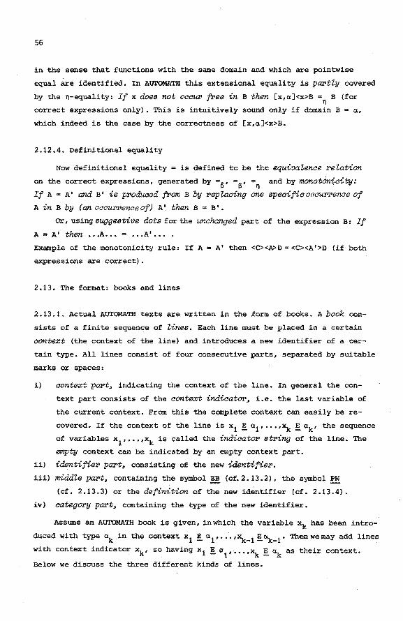
56
in the sense that functions with the same domain and which are pointwise
equal are identified. In AUTOMATH this extensional equality is partly covered
by the n-equality: If x does not occur jree in B then [x,a]<x>B " B (for n
correct expressions only). This is intuitively sound only if domain B =a,
which indeed is the case by the correctness of [x,a]<x>B.
2.12.4. Definitional equality
Now definitional equality = is defined to be the equivalence relation
on the correct expressions, generated by =6, =a• n and by monoton~city:
If A • A' and B' is produced jrom B by replacing one specificoeaurrenae of
A in B by (an oaeurr>enaeof) A' then B = B'.
or, using suggestive dots for the unchanged part of the expression B: If
A= A' then •.• A ••• = ••• A' ••••
Example of the monotonicity rule: If A = A' then <C><A>O = <C><A'>O (if both
expressions are correct).
2.13. The format: books and lines
2.13.1. Actual AUTOMATH texts are written in the form of books. A book con
sists of a finite sequence of lines. Each line must be placed in a certain
context (the context of the line) and introduces a new identifier of a cer
tain type. All lines consist of four consecutive parts, separated by suitable
marks or spaces:
i) context part, indicating the context of the line. In general the con
text part consists of the context indicator, i.e. the last variable of
the current context. From this the complete context can easily be re
covered. If the context of the line is x 1 ! a1 , ••• ,xk !ak, the sequence
of variables x1
, ••• ,xk is called the indicator string of the line. The
empty context can be indicated by an empty context part.
ii) identifier part, consisting of the new identifier.
iii) middle part, containing the symbol EB (cf. 2.13.2), the symbol PN
(cf. 2.13.3) or the definition of the new identifier (cf. 2.13.4).
iv) category part, containing the type of the new identifier.
Assume an AUTOMATH book is given, in which the variable xk has been intro
duced with type akin the context x1 ! a 1 , ••• ,~-l !ak_1• Thenwemay add lines
with context indicator xk, so having x 1 E a , '• •• ,x. E a as their context. - 1 j{- k
Below we discuss the three different kinds of lines.

57
2.13.2. The bZock opening Unes have middle part EB (for empty bZock opener)
or, in alternative notation, a bar -- • An ~-line· introduces a new varia.bZe
and thus allows extension of the current context by one assumption.
Example: ~ * y := EB E a ("let y be of type a") introduces a new variable
y of type a. Lines having y as their context part - which may appear later
in the book- then have x1 ! a 1 , ••• ,~! ak' y! a as their context.
2. 13. 3 • The primitive notion Unes have middle part .!:!! and introduce the
primitive notions. For example:
~ * P := .!:!! .! a
introduces the primitive constant expression p(x1
, ••• ,~) and contains the
axiomatic !_-statement p(x1
, ••• ,xk).! a.
2.13.4. The abbreviation lines look like:
~ * d := D! a ,
where the middle part D is the definition of d, i.e. the expression to be
abbreviated. This line contains, relative to the preceding book and the cur
rent context, both the derived !-statement D .! a and the defining axiom for
the new defined constant d:
2.14. correctness of lines1 validity
A line is correct if both the middle part (if not ~or PN) and the
category part are correct expressions with respect to the preceding book
and the current context, and the category part is the type of the middle
part (if not ~ or PN). For the correctness of the expressions, all identi
fiers used have to be vaU.d. constants are valid in a book from the line on
in which they are introduced. Free variables are valid. in a line if they
occur in its context. We speak ·about the block of lines in which a free
variable is valid (whence block opener).
2.15. Shorthand facility
Assume that a primitive or defined constant c was introduced in a cer
tain context x1 ! a1
, ••• , ~ ! ak. Then if later in the book c occurs with
fewer than k arguments, the argument list is completed by adding a suitable

58
initial segment of the original indicator string (cf. 2.13.1ii)) x1, ••• ,~.
In other words the expression c(Ai+1, ••• ,Ak) is shorthand for
c(x1, ••• ,xi,Ai+l'''''~) and the single constant c is shorthand for
c(x1, ••• ,~). Clearly the completing variables have to be valid, that is,
the initial segments of the original and the current context have to coin
cide. The shorthand facility accords with usual mathematical practice where
free variables are often considered as fixed throughout an argument and are
not mentioned explicitly.
2.16. Paragraph system
For each variable and constant i.t must be possible to retrace from which
line it originates. This condition is clearly satisfied when all names are
unique. A more liberal method of naming however is allowed by the socalled
para~aph system, for a description of which we refer to Zandleven [11,
section 11]. Both shorthand facility and paragraph system do not really
concern the language definition but are present for convenience only.
2 .1 7 • Example
In the following AUT-68 booklet the examples of the preceding sections
are now written in the proper format.
* nat := PN ~ * 1 := PN nat
*X :• -- nat
X * successor :• !!'! nat
* 2 := successor (1) nat
* 3 := successor{2) nat
X * plustwo := successor(successor) nat
* succfun := [x,nat]successor(x} [x,nat]nat
* 3alt := <2>succfun nat
Here the middle part of plustwo uses the shorthand facility. It is left to
the reader to establish 3 = 3alt.

59
3. Mathematics in Atrl'OMATH: Propositions as types
3.1. Functional interpretation of logic
Up till now we have described AUTOMATH as a calculus of objects and
their types only. A major part of mathematics however consists of making state
ments and reasoning with them, i.e. deals with logic.
Now there are different ways of coding some logic into the objects-and
types framework. Here we only mention a socalled fUnctional interp~tation
of logic, whi~h gives rise to thepropositions-as-types notion. This idea of
interpreting logic was developed independently by de Bruijn and certain
others, of whom we mention Howard [6], l?rawitz [10], Girard [5] and Martin
Lof csJ.
3.2. Propositions as types
So far we have introduced~ as the only 1-expression. We had t !~
and r ! t f~ the types t and the objects r of type E respectively. Now we
introduce another !-expression, the basic symbol ~· Originally in AUT-68
no distinction was made between ~ and ~· The latter !-expression acts
just like ~ and was introduced later to allow difference of treatment be
tween types which are to be considered as propositions and types which are
just types of objects.
If E !~we consider t as a proposition. If further r! E , we con
sider r as some construction establishing the truth of t (a "proof" of t).
Thus the formula r E E is conceived as asserting the proposition E.
3.3. Interpreting implication
Let a!~ and a!~· Now we may say we have a "proof" of the im
plication a + 8 if from an assumption of the truth of a we can argue and
conclude the truth of a. That is, if for any construction establishing the
truth of ll we can produce a construction for the truth of a or, equivalently,
if we have a map fran "proofs" of a. to "proofs" of a. Now in AUTOMATE terminology: we say we "prove" a + B if for any x ! a
we can produce some B ! a. I.e. if we have some E in the function type
[x,a]B. So we let [x,a]6 denote the implication a+ Band have [x,a]B !~·
This corresponds to the second interpretation of abstraction expressions in
section 2.9.

60
Now by this interpretation we obtain the modus. ponena (from a and a + B infer 6) by simple functional application. For let A ~ a and E ![x,a]6
{A and I: thus being "proofs" of a and a+ B respectively). Then by the appli
cation rule we construct <A>E establishing the truth of B.
3.4. Universal quantification; negation
In exactly the same manner a function interpretation of universal state
ments can be given. Namely if a~~ and for x ~a we have B ~~then
we identify the function type [x,a]B with the universal statement VxEaB·
Here functional application corresponds to the "instantiation" rule in logic.
Thus by this interpretation of logic in AUTOMATH one gets the {V,+)
fragment of first order predicate logic for free. However in AUTOMATH only
positive statements are made and statements like: "E is not of type r" cannot
be expressed. In order to interpret negation we introduce as a primitive no
tion the proposition con {for "contradiction") together with some suitable
axiom (primitive notion). Here are different possibilities, e.g. the intu"
itionistic absurdity rule (for any proposition a, from con infer a) or the
classical double negation 'terM. Then an AUTOMATH theory (i.e. book) is con
sistent if, in the empty context, it does not produce some I: ~con.
For a ~~we define non(a) as a+ con or, in AUTOMATS notation,
[x,a]aon. Now the double negation la~ can be stated by introducing the pri
mitive notion dnl as follows: If a~~, x ~ non(non{a)) then dnl(a,x) ~a.
By also choosing suitable definitions for the other connectives (A,v)
and the existential quantifier we can smoothly obtain full classical first
order predicate calculus.
3.5. Assumptions, axians, theorems
In AUTOMATH-books the E-formula r E E for a proposition E can occur in
the usual three kinds of lines again:
i) _!!-lines: a * x :=!!~E.
These must be interpreted as assumptions: "let E hold" or "let x be a
proof of E". Now in a line where x is valid we may refer to x whenever
we want to use the . assumed truth of E •
ii) ~-lines: a * p := PN ~E.
These serve as axioms, or rather as axian schemes (by the dependence
on the variables contained in the context o}.
iii) abbreviation lines: a * d := r E E must be considered as derived state-

61
menta, i.e. theorems, lemmas etc. Here the middle part r "proves" the pro
position E from the assumptions in the context o.
3.6. Book-equality
The definitional equality (cf. section 2.12) of AUTOMATH only covers
a small part of the usual mathematical equality. Further a statement of
definitional equality cannot be handled as an actual proposition; e.g. it
cannot be neqated or even assumed (as in: let A = B). As the AUTOMATH-counter
part of the usual mathematical •• ,equals... the book-equal-ity IS(a,A,B)
- where A and B are objects of type a - can be introduced by suitable pri
mitive notions, some of which are shown in the example below.
* 0.
0. * X
X * y
y * IS
X * REFL
y * 1
1 * SYM
and also:
0. * a B * f
f * X
X * y
y * i
i * ISAXl
:= --:= -:= -:= E!! := PN
:= --:= PN
etc.
:=
:=
:=
!""
:=
:= PN
~
IS(x,xl
IS(x,y)
IS(y,x)
~ [x,o.]l3
a
IS(x,y)
IS(I3,<x>f,<y>f)
'By the axiom of reflexivity (REFL) above, definitional equality implies book;; ':equal1ty: if A! a, B! a., A= B then REFL(a,A) ! IS(a,A,B),

62
4. Extension of AOT-68 to AOT-QE
4.1. Function-like expressions
Expressions E such that E ! [x,a]B or E = [x,a]B are called funation-Zike
expressions. Whereas in AUT-68 function-like 3-expressions may have any form,
e.g. they can be variables or primitive constant expressions, the only func
tion-like 2-expressions are (possibly abbreviated) abstraction expressions.
This is because function-like 1-expressions are absent in AUT-68.
Thus we can discuss explicitly constructed families of types Bx where x
ranges over some type a (namely by forming the abstraction expression
[x,a]B(x]) but we cannot discuss ~bitrar,y families of types indexed by
x ! a. Indeed, we cannot introduce a family of types as a primitive notion
or as a variable.
4.2. Supertypes or quasi-expressions
In AUT-QE such arbitrary type-valued functions are admitted however, by
extending the class of 1-expressions. The new 1-expressions, quasi-~ressions
(whence AUT-QE) or supertypes., have the form [x1 ,a1] ••• [~,ak] ~ or
[x1,a1J ••• [xk,ak] ~' where a 1, ••• ,ak are 2-expressions, i.e. propositions
or types.
For example, an arbitrary type-valued function on a can be introduced by
an EB-line:
cr * f := -- [x,a]~ •
If for a we take the type of natural numbers, then f is an arbitrary sequence
of types.
4.3. The use of AUT-QE.
Similarly we have arbitrary prop-vaZusd funations in AUT-QE. These are
especially useful in our interpretation of logic, for a prop-valuedfunction
with domain a is nothing but a predicate over a. For example, by an EB-line
O*R=-- [x,nat][y,nat]~
an arbitrary binary predicate (rather: relation) on the natural numbers is
introduced, The presence of predicate and relation variables in AUT-QE al
lows us to write aziom schemes with such variables, e.g. to introduce a fur
ther equality axiom (cf. section 3 .6) we can write:
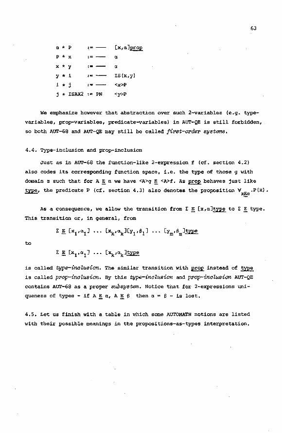
63
a * p ~~ --- [x,a]~
p * X := --- a
X * y := --- a
y * i := ---- IS(x,y}
i * j := <x>P
j * ISAX2 := PN <y>P
We emphasize however that abstraction over such 2-variables (e.g. type
variables, prop-variables, predicate-variables} in AUT-QE is still forbidden,
so both AUT-68 and AUT-QE may still be called first-order systems.
4.4. Type-inclusion and prop-inclusion
Just as in AUT-68 the function-like 2-expression f (cf. section 4.2}
also codes its corresponding function space, i.e. the type of those 9 with
domain a such that for A! a we have <A>g! <A>f. As ~behaves just like
~~ the predicate P (cf. section 4.3) also denotes the proposition VxEa.P(x}.
As a consequence, we allow the transition from t ! [x,a]~ to E ! type.
This transition or, in general, from
to
is called t,ype-inctusion. The similar transition with ~ instead of ~
is called prop-inclusion. By this type-inclusion and prop-inclusion AUT-QE
contains AUT-68 as a proper subsystem. Notice that for 2-expressions uni
queness of types - if A ! a, A ! 6 then a = 6 - is lost.
4.5. Let us finish with a table in which some AUTOMATH notions are listed
with their possible meanings in the propositions-as-types interpretation.

64
AUTOMATH-notions
2-expressions
3-expressions
• •. E •. •
function-like
2-expressions
EB-lines
E!-lines
abbreviation lines
object-and-type
interpretation
types
objects
••• has type •••
{
type-valued functions
function types
variable introductions
primitive object
introductions
definitions or
abbreviations
proof- and- proposi
tiOn interpretation
propositions
proofs
••• proves
predicates
{
implications
universal statements
assumptions
axioms
theorems

5. A formal definition of AUT-QE
5.1. The language, to be defined formally now, is the one accepted by the
current checker (cf. [11]) except for two points:
i) Paragraph facilities are not present here so all constant names have
to be distinct (cf. section 2.16).
ii) There is no shorthand facility (i.e. all expressions are written out
in full (cf. section 2.15).
65
The actual formalism has been chosen in this way in order to keep as close
as possible to the preceding informal book-and-line description. A defini
tion along more usual natuvaZ deduction lines may possibly be more elegant.
For technical reasons we preferred to avoid redundancy almost completely
in our definition. As a consequence of this, some useful extra rules follow
as derived ruZes in the section on language theory.
5.2. Our aim is to define formally what correct AUT-QE books are.
The description consists of:
i) Preliminaries, mainly devoted to the context free part of the language
(section 5.4).
ii) SimuZtaneous definition of correctness of books, contexts, lines, ex-
pressions, ~-formulas and ~-formulas (section 5.5).
The m-formulas only serve as a help in our definition; they do not appear
in the book. The kernel of ii) is the definition of correctness of expres
sions and formulas relative to a certain book and context. Here the book
serves to determine the set of primitive notions and abbreviations, and the
context serves to determine the set of valid free.variables.
Most concepts are introduced by ordinary induative definitions. These con..:.
sist of a finite set of rules of the form: "if ••• then ••• ". Here only such
conclusions may be drawn which follow from a finite number of applications
of the rules.
5.3. Notational conventions
5.3.1. An extensive use is made of ayntaatia variabZes throughout the definition.
Often certain assumptions on these variables are implicit by their specific
choice, e.g. cr and ~ always run over contexts. Syntactic variables may al-
ways be indexed or primed.

66
5.3.2. As for substitution and a-conver>sicm (renaming of bound. variables)
we adopt the following point of view: expressions.fith bound variables are
considered as named versions - named to facilitate reading - of some actually
namefr>ee skeleton (cf. [3]). Thus we identify a-equal expressions and assume
that a-conversion is applied whenever necessary to avoid clash of variables.
We use ••• :: ••• to denote ayntaatia identity (symbol-for-symbol equality)
modulo a-equality. E.g. [x,I:] ... x ... :: [y,E] ... y ... y ....
5.3.3. Correctness of expressions A and formulas ~ relative to a book 8 and
a context o are abbreviated by 8; a ~ A and B; a 1- ~ respectively. Sometimes
we write ~ A or a ~ A for 8; a ~ A and ~ ljl or o ~ ljl for 8; o ~ ljl when there
is no particular need to emphasize the current book or context. The notations
~(i}A and ~(i)A E Bare used to express that A is ani-expression and ~A (respectively ~A~ B).
5.4. Preliminaries
5.4.1. Alphabet
1) As variables and constants we allow any atphanumer>ia st:t>ing. SUch a string
is considered atomic and is thus counted as one single symbol. Syntactic
variables for variables are x,y,z, •••• Among the constants (syntactic va
riable c) we distinguish p:t>imitive (syntactic variable.s p,q) and defined
or abbr>eviationat constants (syntactic variable d).
2) Improper symbols
i) some b:t>ackets and br>aces: [ , ], ( , ), < , >,
ii) Some separ>ation mar>ks: ! , *, ~~ ~· :=, =, aemiaoton and aomma.
iii) Some r>ese:t>Ved symbols: !!!_, PN.
5.4.2. Expressions (syntactic variables A,B,C,D, ••• ,E,A,r, ••• )
i) V ar>iab tes : x
ii) Abst:t>aation e:x:pr>essions: [x,E]A
iii} Apptiaation e:x:pr>essions: <E>A
iv) Constant-expr>eseion instanaea: c(E1
, ••• ,Ek)
v) Basic aonstants: ~· ~·
As special syntactic variables for 2-expr>essions we take a,~, ••••

5.4.3. Formulas {syntactic variable ~)
i} !_-fOlWI.UZas: E E 1::.
ii) =-fo:r'Tn'Ul.aB: E = !!. •
5.4.4. Additional concepts
67
1) Cont~ts {syntactic variables o,~): Any finite (possibly empty) sequence
of !!:fo:r'Tn'Ulaa xi! Ei, separated by commas, UJhere a'll xi are different.
2) Lines (syntactic variable A}
i) ~-linea
ii) PN-linee
t:1 * X := EB E E
o * p := PN E E
iii) Abbreviation linea: o * d := 1::. E E
3) Books {syntactic variable 8): Any finite (possibly empty) sequence of
lines, separated from one another by e:xc Zarnation signs (!) •
5.4.5. Free variables
We define the free variable set FV(E) of expressions E by induction on
the structure of E (cf. section 5.4.2):
i) FV(x) = {x}
ii) FV([x,r]t:.) = FV{f) u (FV{A)\{x})
iii) FV(<f>l::.) = FV(r) U FV(I::.)
iv) FV(c(E 1, ... ,Ek}) = ui=l, ... ,kFV(Ei)
v} FV(.e.e£) • FV(~ = fi',
5.4.6. Substitution
1) The result of simultaneous substitution of A1
, ••• ,~ for the free varia
bles x 1 , ••• ,~ in an expression E is denoted by [x1 , •••• ,~/A1 , ••• ,~DE
and locally abbreviated by r*
i)
ii)
iii)
iv)
v)
vi)
* xi ;: Ai
y* = y if y not among x1 ,.~.,~ * * * ([y,E 1 JE 2 l == [y,E
1 ]E 2 if ynot among x
1, ... ,~ and
x1
€ FV(E 2).,. y rf FV(Ai)) fori= 1, •.• ,k (otherwise rename y in
[y,E1]E2).
* * * (<E1>E2) : <E1>E2
* * * (c(I:1, ... ,iln}) :: c(E1
, ... ,Em)
* * .e.e£ = .e.e£• ~ = ~-
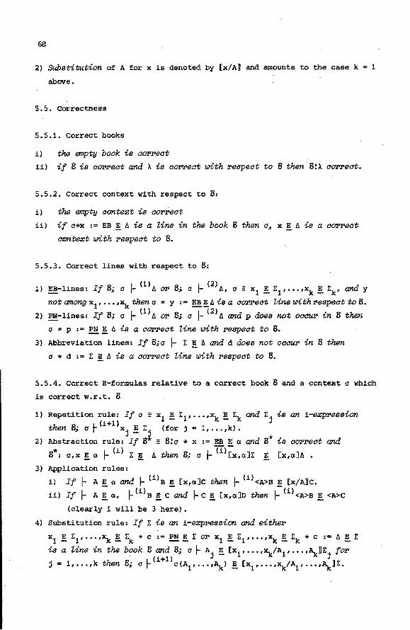
68
2) Substitution of A for x is denoted by (x/AD and amounts to the case k .. 1
above.
5. 5. Correctness
5.5.1. Correct books
i) the empty book is aot>t>ect
ii) if 8 is aOl'l'ect and i\ is COl'l'eat with t>espeat to 8 then 8:i\ COl'l'ect.
5.5.2. Correct context with respect to 8:
i) the empty con~t is aol'l'eat
iil if a*x := EB ~ 8 is a Zine in the book 8 then a~ x ! 8 is a col't'eat
contea:t with t>espeat to B.
5.5.3. Correct lines with respect to 8:
l) !!?_-lines: If 8; a 1- (1)8 Ol' B; cr 1- (2 >A, a:: x1
! I:1
, ... ,~! I:k, and y
not among x 1, ... ·~then a * y := !!?_~A is a col't'eat Zine witht>espect to B. 2) PM-lines: If 8; a 1- (1) t. 01:' 8; a 1- {2) 8 and p does not oaCUl' in 8 then
a * p , .. .!:!!. ! t:. is a eOl'l'ect Zine with Nspect to B.
3) Abbreviation lines: If B;a 1- I: ! A and d does not OCC'Ul' in 8 then
a * d := I: ! A is a cot>t>eat Zine with t>eapeet to B.
5.5.4. Correct E-formulas relative to a correct book B and a context a which
is correct w.r.t. 8
1) Repetition rule: If a -then B· a 1-(i+l)x E I:
~ j - j
x1 ~ I:1, ••• ·~ ! I:k and I:j is an i-ea;pl'eaaion (for j = 1, ••• 1kJ.
2) Abstraction rule: If B* = B:a s*; a,x!a 1-(i) I:! t. then
* X := EB E a and 8* is COl'l'ect and
I Til-8; a - [xla]I: ! [x,a]t. •
3) Application rules:
i) If 1- A ! a and j- {1) B ! [x,a]C then 1- (i) <A>B ~ [x/A]C.
ii) If 1- A ! a, r (i) B ! C and 1- C ~ [x 1 a]D then 1- (!) <A>B ! <A>C
(clearly i will be 3 here).
4) Substitution rule: If I: is an i-ea;pt>ession and either
x 1 ~ I:1 1 .. • ·~! I:k * c := !!!, ! I: or x1 ! 1: 1 1 ... ,xk ! Ik * c :• 8 ! I:
is a tine in the book 8 and B; a r Aj ! [x1 I ••• ·~/Al, ••• ,~]I:j for L (i+l)
j .. l 1 ••• 1 k then B; a r c(A1
, ... ,~)! [x1
, ... ,~/A1 , •• .,~)I:.

5) Rule of type-conversion: If 1- 11 !, l: and 1-1: = r then l-1:!. !, r. 6) Rules of type- and prop-inclusion:
i) If 1- E !. [x1 ,a
1] ••• [xk,ak][y,S] ~ (possibly k = 0) then
j- E !. [x1,a1 ] .•• [~,ak]~.
ii) If 1- I: !. [x1 ,a
1] ... [~,ak][y,S]~ (possibly k = 0) then
~ E ! [x1 ,a1] ••• [~ ,ak]~.
5.5.5. Correct expressions with respect to 8 and o
1) Correct !-expressions:
69
i) If B is aorl"eat and o is ao!'l'eat with NSpect to 8 then 8; o 1- (l) SfE!. and 8; 0 1- (l)~·
ii) Ifs* = 8!a *X := EB!. a and B*; a,x!. a ~(l) 1:!. then 8;a 1-(l)[x,a]l:i..
2) Correct 2- and 3-expressions: If 1- (i) E !. 1:!. then I- (i) E •
~: It is intended that 8; o j- A or 8; a j- q1 only if 8 is correct and o
is correct with respect to B. This condition is explicitly imposed in 5.5.4
and S.S.S.li) and propagated all through the definition.
5.5.6. Correcti=-formulas with respect to B and a '
1) B-equality: If I- <A>[x,a]B and j-[x/A]B then j-<A>[x,a]B = [x/ADB.
2) n-equality: If Hcx,B]<x>C, and X t FV(C) and 1-c then ~[x,B]<x>C = c. 3) o-equality: If x1 !. E1 , ••• ,~!. I:k * d := 1:!.!. Eisa line in B~ and
B; a 1-Aj!. [x1 , ••• ,xk/A1, ... ,Ak]l:j for j = l, ... ,k, and
B; a j-[x1 , ... ,~/A1 , ... ,~Dl1 then 8; o l-d(A1 , ... ,"\:) = [x1, ••• ,~/A1 , ... ,~Dl1
4) Monotonicity rules:
1) If s* = B!a * X := E:S)ka and B*; a,x E a 1- Bl = B2 then -~, -
8; a j- [x,o:Js1
= [x,a]s2 :"
ii) If 1- a 1 = a2
, j-[x,a1
]B, and 1- [x,o:2Js then 1- [x,a
1 ]B = [x,a
2JB.
iii) If j- A1 = s1
, j- A2 = s2 , j- <A1>A2 , and~ <B1>s2 then 1- <A1>A2 = <B1>s2 •
iv) If j- Aj Bj {for j = l, ... ,k), and l-c{A1
, ... ,~), and
1- c (Bl I ••• ,Bk) then 1- c (Al, •• .,~) .. c {Bl I ... ,Bk).
5) Reflexivity, symmetry and transitivity rules
i) If j- A, j- B and A :: B then j- A = B
ii) If j- A = B then j- B = A
iii) If j-A = B, and j- B = C then j-A =C.
70
~; It is intended that 8; a ~ A = B only if both 8; a ~ A and 8; a ~ B.
In most cases above, ,though sometimes unnecessary, such conditions have been
explicitly stated. Where they have been omitted it will be immediate that
they hold by some other conditions.

71
6. Some remarks on language theory
6. 1. Decidabili ty
The language theory is mainly concerned with the investigation of the
basic system. A major aim is to prove the deaidabiUty of the AUTOMATH
languages. That is, to prove the existence of an effective procedure which
for any given text in a finite amount of time decides whether it is correct
or not (in AUT-QE, say) • The kernel of such a checker deals with the veri
fiaation of correctness of expressions and formulas (both !- and =-formulas),
relative to a given book and context (which are assumed to be correct al
ready).
In this section we shall sketch a certain checking procedure, closely
related to the actually running verifying program of Zandleven (cf. [11]).
We shall also roughly indicate the proof of correspondence between the pro
posed checking procedure and the language definition of the preceding section.
6. 2. Reduction
6.2.1. In order to study the =-relation in more detail we introduce the re
duction reZ.ation ~ .. a partial order among the expressions. For an explanation
of the suggestive dots in our definition we refer to section 2.12.4.
6.2.2. Definition:
1) One-step reduction (with respect to a book 8)
i) one-step a-reduction: ••• <A>[x,a]C ••• >a ••• (x/A]C •••
ii) one-step n-reduction: If x I. FV(C) then ••• [x,a]<x>c ••• > ... c ...
iii) one-step 6-reduction: If d z.1as int;roduaed by an abbreviation Zine
x1 ! a1 , ••• ,~! ak * d := D! L in B then ••• d(E1, ••• ,Ek) ••• >0 ••• (x1, ••• ,~/L1 , ••• ,Ek]D •••
iv) also > is allowed with any acmbination of the indices such as: If
A >aB or A >n B then A >an B
v) one-step reduction in general.: If A >Bno B then A> B.
2) Many-step reduction (with respect to 8}
i} If A - B then A ~ B
If A ~ B and B > c (b1ith respect to BJ then A ~ c. So~ is the reflexive and transitive closure of >. Likewise ~So denotes
the reflexive and transitive closure of >So etc. For A ~ B we also write
B SA.

72
3) i) Reduction sequence: A sequence E1,E2 , ••• of expressions is called a
reduction sequence of E1 if for all i we have ·Ei = Ei+l or Ei > Ei+l.
ii) Proper reduction sequence: A ~duction sequence E1
,E2 , ••• is called
proper if for all 1 we have Ei > Ei+l'
6.2.3. Clearly the =- relation is the equivalence relation generated by the
restriction of > to correct expressions. So we can conclude: ~ A = B iff A= c 1 ~ o1 ~ c2 ~ o2 s ••• ~ ok-l s ck = B (possibly k = 1), where all exp~ssiona in the respective reduction sequences are cor.reat.
6.2.4. As an example of a reduction sequence consider:
3ait :>0
<2>succfun >0
<2>[x,nat]successor(x) >a successor·(2) >0
successor(successor(l)) (see section 2.16). So each reduction step seems to
bring us closer to some possible "outcome". Here a- and &-reduction amount
to evaluation and n-reduction to a certain simplification of expressions.
6.3. The three problems: no:rmal.ization, Church-Rosser and closure
6.3.1. It will. appear that the decision procedure for equations {=-formul.as}
plays a central role in the checker. At first we state - in terms of the re
mark in section 6.2.4 - two ~portant questions around reduction and defini
tional equality:
i) (Normalization) Do correct expressions always have a final outcome,
i.e. do they always reduce to an expression which does not reduce further?
ii) (ChuZ'ch-Rosser property) Do definitionally equal expressions have a
common outcome, i.e. an expression to which they both reduce?
A third central question concerns the so-called closure property (this term
was introduced by R.P. Nederpelt in the introduction to [9]}:
iii) Is the system closed under reductions, i.e. do correct expressions re
main correct under reduction?
6.3.2. Normalization and strong normalization
Let us define
1) A is normal if no one-step reduction A > B can be applied.
2) A is said to normalize if A reduces to some normal B {which is then call
ed a no:rrmaZ fo:rrm of A) •
3) A is said to stvongly no:rrmalise if al.l proper reduction sequences of A
terminate.
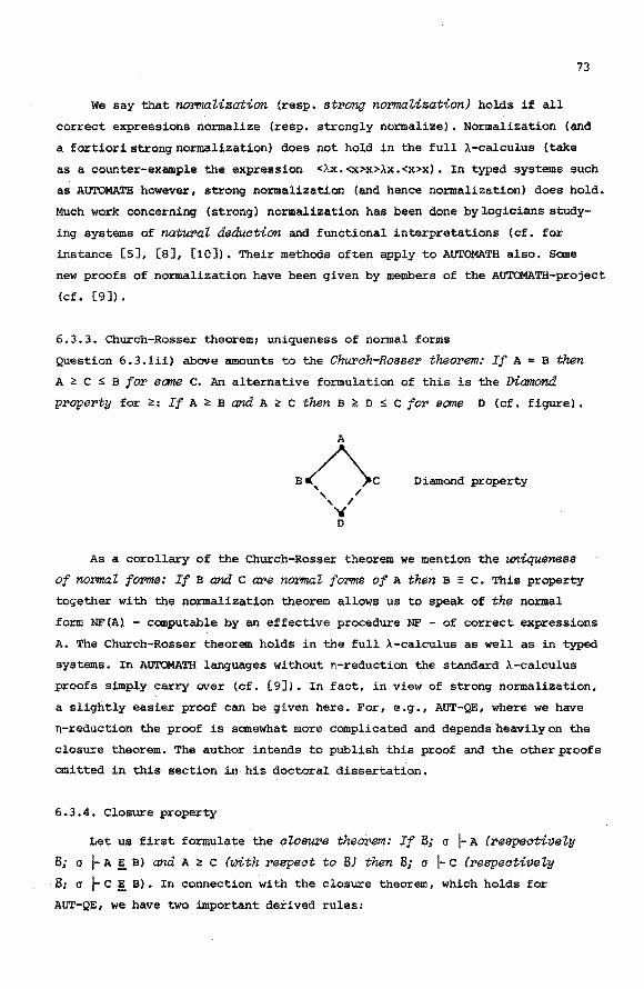
73
we say that normalization (reap. st~ong normalization) holds if all
correct expressions normalize (reap. strongly normalize}. Normalization (and
a fortiori strong normalization) does not hold in the full >.-calculus (take
as a counter-example the expression <>.x.<x>x>>.x.<x>x). In typed systems such
as AUTOMA'l'B however, strong normalization (and hence normalization) does hold.
MUch work concerning (strong) normalization has been done by logicians study
ing systems of natw:>al deduction and functional interpretations (cf. for
instance [5], [8], [10]). Their methods often apply to AUTOMATH also. Some
new proofs of normalization have been given by members of the AUTOMATH-project
(cf. [9]).
6.3.3. Church-Rosser theorem; uniqueness of normal forms
Question 6.3.1ii) above amounts to the Church-Rosse~ theo~em: If A = B then
A :<: c ~ B fO!' acme c. An alternative formulation of this is the Diamond
p~ope~ty for~: If A~ Band A:<: c then B :<: D s c fo~ some D (cf. figure).
Diamond property
As a corollary of the Church-Rosser theorem we mention the uniqueness
of normal forms: If B and c ~e normal forms of A then B = c. This property
together with the normalization theorem allows us to speak of the normal
form NF(Al - computable by an effective procedure NF - of correct expressions
A. The Church-Rosser theorem holds in the full A-calculus as well as in typed
systems. In AUTCMA'l'B languages without n-reduction the standard A -calculus
proofs simply carry over (cf. [9]). In fact, in view of strong normalization,
a slightly easier proof can be given here. For, e.g., AUT-QE, where we have
n-reduction the proof is somewhat more complicated and depends heavily on the
closure theorem. The author intends to publish this proof and the other proofs
omitted in this section in,his doctoral dissertation.
6.3.4. Closure property
Let us first formulate the clo8UI'e theo~em: If B; o ~A (~espectively
B; a ~A !. B) and A ~ c (with respeat to BJ then B; a 1- c (respeatively
B; a r c!. B). In connection with the closure theorem, which holds for
AUT-QE, we have two important derived rules:

74
1) General, substitution prineipte (as mentioned in 2.5): If
x1 !.. I:1, ••• ·~!. l:k ~ B (resp. ~ B! C) and a 1-Ai.!. I:: (for i = 1, ••• ,k)
I * I * * * then a - B (resp. r B !. c ) , where I: stands for [x1, ••• ,~/A1 , ••• ,~]I:.
2) The "Zeft-ha:nd equaZi ty ru'le 11 (compare with the rule of type-conversion,
which is the "right-hand equality rule"):
If~ (3)A!. Band J-A = C then J-c !_B.
For 2-expression A we only have a weaker version in view of type-inclu
sion: If ~ (2)A!. Band ~A= C and j- (2)c! D then 1-c! B O'l' f-A! D.
6.4. A decision procedure
6.4.1. Deciding =-formulas
Suppose A and B are correct expressions. The normal form procedure NF
(section 6.3.2) easily yields a decision method for the equation A = B,
namely A = B iff NF (A) : NF (B) • Often, however, it is not necessary to com
pute normal forms for deciding A = B. For example, when A and B have different
degrees one can easily draw a negative conclusion. Or more important, it ge
nerally happens that a few well-chosen reduction steps in A or B will result
in a non-normal common reduct. The choice of efficient reduction steps here
is a matter of strategy; .the termination of a procedure which successively
applies reduction rules to A or B is anyhow guaranteed by the strong normali
zation property, no matter in what order the reduction steps are applied.
In order to prove the correspondence between decision procedure and
language definition we must know that all the expressions in the reduction
sequences from A and B to some common reduct are correct again. This is
indeed the case by the c~osure theorem.
6.4.2. Deciding !_-formulas and epxressions
6.4.2.1. Assume B is a correct book and a a correct context; we must define
a decision procedure for the correctness of !_-formulas and expressions. It
will appear that this problem can be reduced to the decision problem for
=-formulas (but for the straightforward task of checking the validity of
the identifiers used) •
6.4.2.2. Uniqueness of types
We know (by the rule of type conversion) that for all B' with ~ B = B'

we have 1- A !!!, B * 1- A ! B 1 •
For 3-expressions A the converse (uniqueness of types*) holds too:
( *) 1- A! B and f- A! B' • 1- B = B'.
For 2-expressions A we must be somewhat more precise in view of type-in
clusion. We define among the correct expressions the relation ~ by:
i) [xl'a1J ••• [~,ak)[y,l3]~ c [x1,a1J [~,ak]~ ii) [xl,al] ••• [~,ak](y,aJ~ c [xl,al] [~,ak]~ iii) ~ is the transitive closure of = and c.
Then instead of (*) for 2-expressions A we can prove
f-( 2)AE!,B and I-(2)A!B 1 -1-B:; B' 02' 1-B' =.B.
75
6.4.2.3. Now assume that A is correct. Then we can define a "mechanical type"
function CAT, such that:
i) 1- (3)A! B * 1- (3)A, 1-B and 1-CAT(A) B
ii) 1- (2) A ! B +9 1- (2) A, 1- B and 1- CAT(A) £. B.
so CAT computes some canonical representative of the class of B' with
1- A ! B 1 ; furthermore, this B' is minimal with respect to £.. For the actual
definition of CAT we refer to [11, section 7]. Since the decision procedure D = for equations in the current checker also contains the possibility of
D type-inclusion- i.e. A • B iff A£. B- the type function CAT reduces
the verification of !-formulas to the verification of equations.
6.4.2.4. Finally we point out a decision procedure for correctness of ex
pressions. Here we proceed by induction on the length of expressions. As an
example we treat the case of application expressions <A>B where A and B are
already supposed to be correct.
6.4.2.5. Uniqueness of domains
For function-like expressions A we define a to be the dOmain of A if
*) Here we mean uniqueness with respect to definitional equality (=), in con
trast with section 6.3.3, where we mean uniqueness with r~spect to syntac
tic equality(:).
76
~ A! [x,a]E 01." 1- (1} A = [x,a]E •
For domains we have uniqueness also (by the closure theorem and the
Church-Rosser theorem) : If a and a a:.re domains of A the.n a = a. This fact
allows us to speak about the domain of function-like expressions. Now we
are able to define a ''meahaniaal domain 11 function OOM (for which we refer
to [11, section 7]), which for function-like A picks out a canonical repre
sentative of the domajn of A. The termination of OOM(A) follows by induction
on the degree of A, using strong normalization.
6.4.2.6. By CAT and DOM the verification of correctness of <A>B reduces to
the verification of some suitable equation: ~<A>B.,. ~ A and 1- B and
~A !DOM(B) or, equivalently, by 6.4.2.3i),
~<A>B .,. ~ A and 1- B and 1- CAT (A) = DOM (B) •
6.4.2.7. For the other cases of correctness of expressions we refer to Zand
leven again. The correspondence of the current verifier with the actual
language definition is either immediate or follows from the above facts
about CAT and DOM.

77
7. References
[1] De Bruijn, N.G.; The mathematical language AUTOMATH, its usage and
some of its extensions. Symposium on Automatic Demonstration
(Versailles D~cember 1968), Lecture Notes in Mathematics, Vol. 125,
pp. 29-61, Springer-Verlag, Berlin, 1970.
[2] De Bruijn, N.G; Automath, a language for mathematics; notes (prepared.
by B. Fawcett) of a series of lectures in the S~inaire de Mathe
matiques SUperieures, Universite de Montreal, 1971.
[3] De Bruijn, N.G.; Lambda calculus notation with nameless dummies, a
toot for automatic formula manipulation, with appUaation to the
Church-Rosser theorem, Indag. Math., 34, no. 5. 1972.
[4] De Bruijn, N.G.; The AUTOMATH Mathematics Checking P!'ojeat, this volume.
[5] Girard, J. Y.; Interpretation fonationeUe et elimination des coupures
de l'arithmetique d'ordre superieur, Doctoral dissertation, Uni
versite Paris VII, 1972.
[6] Howard, w.A.; The fo:rmuZae-as-typee notion of aonstruction, unpublished
1969.
[7] Jutting, L.S. van Benthem; The development of a text in AUT-QE, this
volume.
[8] Martin-Lof, P.; An intuionistia theory of types, unpublished 1972.
[9] Nederpelt, R.P.; Strong nonnalization in a typed tambda-oaloulus with
'lambda-structured types, Doctoral dissertation, Technological
University, Eindhoven, 1972.
[10] Prawitz, D.; Ideas and results in proof theory, in: Proc. 2nd. scan-
dinavian Logic Symp. North-Hollimd Publ. Comp., Amsterdam, 1971.
[ 11 ] Zandleven, I. ; Verifying program for AUTOMATH, this volume.
73
Appendix 2; The paragraph system
In the definition of AUT-QE ([vD, 5]) it is required that constants
which are identifier parts of different lines are different. In this appen
dix we describe a variant of AUTOMATH languages in which this rule is wea
kened. The AUT-QE version of this variant has actually been used for trans
lating Landau's book. It is irrelevant for the following discussion, which
particular AUTOMATH language is considered. We shall therefore presuppose
unspecified language AUT, and we shall call its paragraphed variant AUT-PAR.
1. Paragraph lines
A book in AUT-PAR can be split up into paragraphs. In the language
we have three special symbols +, - and -, and a countable set of para
graph identifiers (which we shall denote here by syntactic variables
s,sl,s2, ••• ,t,t1,t2, ••• ). There is a basic paragraph identifier cover • This will play the role of the empty environment; the word "cover" is meant
to suggest "bookjacket". Besides ordinary AU'l'OMATH lines (which we will call
here proper lines), we have a special sort of lines (called paragraph lines),
which are used to indicate the paragraphs. There are two kinds of paragraph
lines: opening lines which have the form +s, and atosing lines which consist
of the single symbol
2. First rule for paragraph lines
For this description we shall number the lines of our book (proper
lines as well as paragraph lines) in their proper order, and we will indi
cate lines by their numbers. For each line n we define o(n) (c{n) respecti
vely) to be the number of opening lines (closing lines respectively) prece
ding it.
The first rule for paragraph lines is:
o(n) ~ c(n) for all n.
It follows that the paragraph lines provide the book with a kind of nested
structure.
The paragraph level of a linen is defined by pl(n) = o{n) - c(n). For
a line n with pl ( n} > 0 we define its paragraph opening by
po(n) = max{m m< nand pl{m) < pl(n)}. It is easy to see that pl(l) = 0,
that for each n with pl(n) > 0 the line po(n) is an opening line, and that
pl(po(n)l = pl(n) 1.

79
3. An example
As an example we represent schematically a book with paragraphs. The
numbering of the lines in the book appears to the left. It only serves our
(metalingual) discussion, and does not belong to the schematically indica
ted AUTOMATS text. The proper lines are indicated by t~eir identifiers (con
stants or variables) and their contexts. The dots indicate middle parts and
category parts.
1
2
3
4
5
6
7
8
9
10
11
12
13
14
15
16
17
18
19
20
+s
+t
+t
+S
+t
* *
* X *
*
X * *
*
*
* X *
a .-b .-
X .- -- E a := X != -- E
c .-a :=
c :=
c .-
X ·- - E .-d :=
In this example we have indeed o(n) ~ c(n) for· all n, and e.g.
o(4) = 1, c(4) = 0 hence pl(4) = 1
o(16) =3, c(16) =3 hence pl(16) =0
po(4) = 3
po (15) = 13
po(20) =17.
80
4. Indices and paragraphs
For references to paragraphs we use indiaes. An index has the form
s 1 - s2 - ••• - su (with u ~ 1). The sign- is used as a separator, and has
nothing to do with the of closing lines. As a syntactic variable for in-
dices we use s. If s = s 1 - s 2 - ••• - su then s - s denotes s 1 - s 2 - ••• -su-s.
For each line n we define an index ind(n) as follows:
if pl(n) 0 then ind(n) = cover.
if pl(n) > 0 and po(n) = +s then ind(n) ind(po(n)) - s.
Note that, by this definition, for each n the first paragraph identifier in
ind(n) is cover Indices of the form cover-s2 - ••• - su are called aorrrpZete
indiaes. So, for all n, ind(n) is complete.
In the example we have:
ind(3)
ind(4)
ind(9)
cover cover - s cover - s - t
ind(15) = cover - t
Given a book B and an index s, the subsequence of B consisting of those
lines n for which ind(n) = s is called the paragraph of s. Note that para
graphs are mutually disjoint.
In our example the paragraphs are:
for s -for s -for s -
-for s -
cover cover cover cover
s
s - t
t
1,2,3,12,13,16
4,5,6,7,11,17
8,9,10,18,19,20
14,15.
If n is a line in a paragraph, and pl(n) > 0 then the line po(n) is
called an opener.ofthe paragraph. Note that the openers of a paragraph are
not lines of that paragraph. The first opener of a paragraph is called the
paragraph opener of that paragraph, the other openers are called reopeners.
The closing lines in a paragraph are called the aZosers of that paragraph.
In our example we see:
-for s = cover - s the paragraph opener is 3, a reopener is 16 and a clo-
ser is 11.
for - cover t s = - s - the paragraph opener is 7, a reopener is 17 and
closers are 10 and 20.
for s = cover - t the paragraph opener is 13 and a closer is 15.
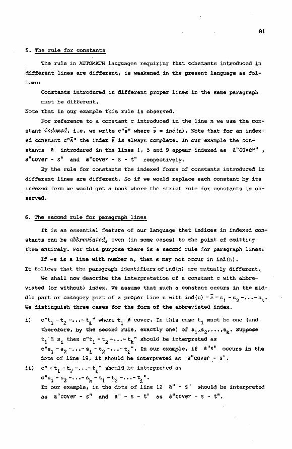
81
5. The rule for constants
The rule in AUTOMATE languages requiring that constants introduced in
different lines are different, is weakened in the present language as fol
lows:
constants introduced in different proper lines in the same paragraph
must be different.
Note that in our example this rule is observed.
For reference to a constant c introduced in the line n we use the con
stant inde:r:ed, i.e. we write c"s" where s = ind(n). Note that for an index
ed constant c"s" the index s is always complete. In our example the con
stants a introduced in the lines 1, 5 and 9 appear indexed as a"cover" , a"cover - s" and a"cover - s - t" respectively.
By the rule for constants the indexed forms of constants introduced in
different lines are different. So if we would replace each constant by its
indexed form we would get a book where the strict rule for constants is ob
served,
6. The second rule for paragraph lines
It is an essential feature of our language that indices in indexed con
stants can be abbreviated~ even {in some cases) to the point of omitting
them entirely. For this purpose there is a second rule for paragraph lines:
If +s is a line with number n, then s may not occur in ind(n).
It follows that the paragraph identifiers of ind (n) are mutually different.
We shall now describe the interpretation of a constant c with abbre
viated {or without) index. We assume that such a constant occurs in the mid
dle part or category part of a proper linen with ind(n) =s=s1 -s2 - ... -sk.
We distinguish three cases for the form of the abbreviated index.
i) c"t1 - t 2 - ••• - t1
" where t1
"f; cover. In this case t 1 must be one (and
therefore, by the second rule, exactly one) of s 1,s2, ••• ,sk. Suppose
t 1· = si then c"t1 - t 2 - ••• - ~" should be interpreted as
c"s1 -s2 - ••• -si -t2 - ... -t.t"• In our example, if a"s" occurs in the
dots of line 19, it should be interpreted as a"cover- s".
ii) c" ~ t 1 - t 2 - ••• - tt" should be interpreted as
c"s1 -s2 - ••• -sk-t1 -t2 - ••• -t.t"•
In our example, in the dots of line 12 a" - s" should be interpreted
as a"cover- s" and a"- s- t" as a"cover- s- t".

82
iii) c appears without index. Then c should be interpreted as c"t" where t
is the "longest possible initial part of s". I.e.: If c is identifier
of a line preceding n in the paragraph of s then c should be interpre
ted as c"s", else if c is identifier of a line preceding n in the para
graph of s 1 - s2 - ••• - sk-l then c should be interpreted as
c"s1 -s2 - ••• -sk-t" etc.
In our example, in the dots of line 4, a should be interpreted as
a"cover" , while in line 6 a should be interpreted as a"cover - s" Note that in the middle part or category part of line 9 a should
again be interpreted as a"cover - s" (i.e. the identifier introduced
in line 5).
We see that the interpretation of a constant with abbreviated index
depends on the place in the book where it occurs.
7. Reference to variables
According to the definition of AUT-QE, variables x1, ••• ,~ of a context
x1 ~ a 1, ••• ,~! ak ~ust be mutually different identifiers. We maintain this
rule in AUT-PAR. Thus free variables occurring in the middle part or catego
ry part of a line always refer to a (unique) variable of the context (Cf.
[vD, 2.4, 2.13.2, 5.5,2, 5.5.3]), Therefore such variables are never indexed.
For variables there are in AUTOMATH no restrictions to their use as
identifier parts of different lines. If a variable x appears as a aontext
indiaator ([vD, 2.13.1 i)]) of a line n it always refers to the latest EB
line introducing x which precedes n. In AUT-PAR a context indicator must be
indexed and for the indexed variables we allow the same abbreviation rules
as in section 6. Hence the context indicator X in line 5 of our example
should be interpreted (according to 6 iii) above) as x"cover - s" i.e.
the variable introduced in line 5. The context indicator X in line 8 should
also be interpreted as x"cover ~ s" , but i:t refers to the variable intro
duced in line 6. In fact in lines n with n > 6 there is no possibility to
use the variable X introduced in line 4 as a context indicator. The con
text indicator X in line 19 should be interpreted as x"cover - s - t" , thus referring to the variable introduced in line 18.
If we want to write line 19 on the context introduced in line 6 we
should write:
19 x"s" * d := ••••.
or, with a complete index:
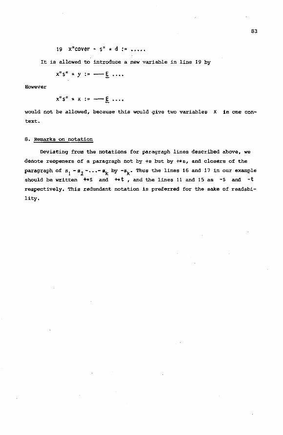
83
19 x"cover - s" * d :=
It is allowed to introduce a new variable in line 19 by
x"s" * y := -- E
However
x"s" * x := --.[ ....
would not be allowed, because this would give two variables X in one con-
text.
8. Remarks on notation
Deviating from the notations for paragraph lines described above, we
denote reopeners of a paragraph not by +s but by +*s, and closers of the
paragraph of s 1 - s2 - ••• - sk by -sk. Thus the lines 16 and 17 in our example
should be written ~s and +*t , and the lines 11 and 15 as -s and -t respectively. This redundant notation is preferred for the sake of readabi
lity.

84
Appendix 3. The PN-lines from the preliminaries
LAYOUT FROH FILE l EXCERPTOUTPUT/PREPNS JANUARY 25r 1977 10148141
+L
*A ,. PROP A * B I• PROP B a IHP I• CXrAJB PROP
a CON I• PH PROP A a NOT , .. IHP<CON) PROP A * WEL I= NOT< NOT< A)) PROP A a W I= WEL<A>
2 W a ET I= PH A B * EC I= IHP<ArNOT<B)) PROP B a AND :· HOT<EC!ArBH PROP
a SIGHA I= TYPE SIGHA a P I• CXrSIGHAJPROP
P a ALL , .. p PROP P a NON I= CXrSlGHAJHOT<<X>P> CXrSIGHAJPROP P * SOHE I= NOHNON(P)) PROP
+E
SIGHA * s I• SIGHA S a T I• SIGHA
3 T a IS la PM PROP 4 S * REFIS I• PN JS(SrS)
p * s I• SIGHA S a T I• SIGHA T a SP I• <S>P
SP * I I• JS(SrT> 5 I * ISP :• PN <T>P
P a AI10NE :- CXrSIGHAJCYrSIGHAlCUr<X>PJCVr <Y>PJJS(XrY> PROP
P a ONE I= AND<AHONE<SIGHArP)r SOHE<SIGHArP)) PROP
p * 01 I• ONE<SIGHArP) 6 01 a IND .,. PN SIOHA 7 01 a ONEAX I• PN <IND>P
SIGHA a TAU I• TYPE TAU * F I• CXrSIGHAJTAU
F * INJECTIVE I• ALL(CXrSIGHAJALL<CYrSIGMAl lHP<JS(TAUr<X>Fr<Y>F>riS<XrY>) )) PROP
F a TO I= TAU TO * IHAGE I= SOHE<CXrSIGHAliS<TAUrTOr<X>F>> PROP
TAU * F I• CXrSIGHAJTAU F * G I• CXrSIGHAJTAU 0 * I I• CXrSlGHAJIS<TAUr<X>Fr<X>G)
8 I a FISI I• PM IS<CXrSIGHAJTAUrFrG) 9 P a OT I• PN TYPE
p * 01 I• OT 10 01 a IN I= PM SIGHA 11 01 * INP I• PN <lN>P 12 P a OTAX1 I• PM INJECTIV£(0TrSIGHArCXrOTl
IN< X>> p * s I• SIGHA s *SI" I• <S>P
13 SP a OTAX2 I• PN IHAGE<OTrSIGHArCXrOTJIN<X>rS) 14 TAU a PAIRTYPE I• PN TYPE
TAU a S I• SIGHA S a T I• TAU
15 T a PAIR I• PN PAIRTYPE TAU a P1 I• PAIRTYPE
16 Pl * FIRST I• PM SIGHA 17 Pl * SECOND ,. PM TAU IS Pl a PAIRISl ,. f"N lS(PAIRTYPErPAIR<FIRSTr
SECONDhP1) 19 T * FIRSTIS1 ,_ PM IS<SIGMArFIRST<PAIR)rS) 20 T * SECONDISl ,. PM IS<TAUrSECOND<PAIR)rT)
-E

+*E
+ST
21 SIGI'IA * SET SIGifA * S
s * so 22 SO * ESTI 23 P * SETOF
p * s S * SP
24 SP * ESTII S * E
25 £ * ESTIE SIGMA * SO
SO * TO TO * INCL
TO * I I * .J
26 .J * ISSETI
-ST
-E
-L
,. ,. t= I• I• I• I• ,. I• I•
=· I• I•
I• I• :•
85
PN TYPE SIGHA SET
PN PROP PN SET
SIGifA <S>P
PM ESTI<S•SETOF<P>> ESTI<S•SETOF<P>l
PN <S>P SET SET
ALL<CXtSIGMAJIKP<ESTI<X•SO>• ESTI<X•TO))) PROP
INCL<SO,TO> INCUTOrSO>
PN IS<SET•SOrTO)

86
Appendix 4. Excerpt for "Satz 27"
LAYOUT FROH FILE EXCERPTOUTPUT/SATZ27 JANUARY 25r 1977 10158122
+L
* A I• PROP A * 8 I• PROP 8 * IHP I• CX•Al8 PROP 8 * Al I• A
Al * I I• IHP<Ar8) I * HP I• <Al>I 8 8 * c I• PROP c * I I• IHP<Ar8) I * J I• IHPC8rC> J * TRIHP I• CXrAJ«X>I>J IHP<ArC)
* CON I= PN PROP A * NOT I= IHPCCON> PROP A * WEL I= NOT< NOT< A>) PROP A * Al I= A
Al * WELI I= CXrNOT<A>J<Al>X WEL<A> A * w I" WEL<A> w * ET I= PN A A * Cl I= CON
Cl * CONE I= ET<CXrNOT<A>JCl> A
+I HP
8 * I I• IHP(Ar8) I * J I• IHP<NOT<A) r8) J * THl I= ET<8rCXrNOT<8>J<<TRIHP<CONrir
X»J>X> 8 8 * N I= NOT< A> N * TH2 I= TRIHP<CONr8rNrCXrCONJCONE<8rX)
) IHP<Ar8) 8 * N I• NOT<B> N * I I= IHP<Ar8) I * TH3 := TRIHP<CONrlrN) NOT<A> B * Al I• A
Al * N I• NOT<B> N * TH4 I• CXriHP<Ar8)J<Al>TH3<N•X> NOT< IHP<Ar8)) 8 * N I• NOT<IHP<Ar8)) N * TH5 I• ET<CX,NOT<A>J<TH2<X>>N> A N * TH6 I• [X,8J<CY•AlX>N NOT<8>
-IHP
8 * EC I• IHP<A•NOT<8)) I PROP
+EC
8 * I I• IHP<A•NOT<8)) I * THl I• I EC<A•8> 8 * I I• IHP(8,NOT<A)) I * TH2 I• CX•Al[Y,8J<X><Y>I EC<A•8>
-EC
8 * E I• EC<A•8> E * Al I• A
Al * ECEl I= <Al>E NOT<8> E * 81 I• 8
81 * ECE2 I= TH3'-IHP'<NOT<8>•WELI<B•8l>•E> NOT< A>
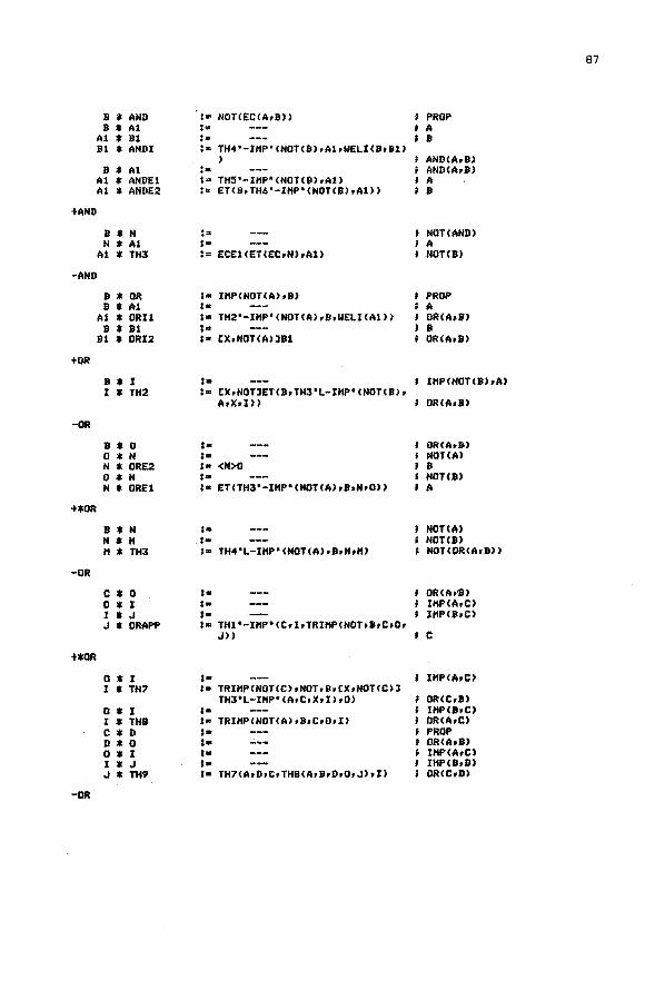
87
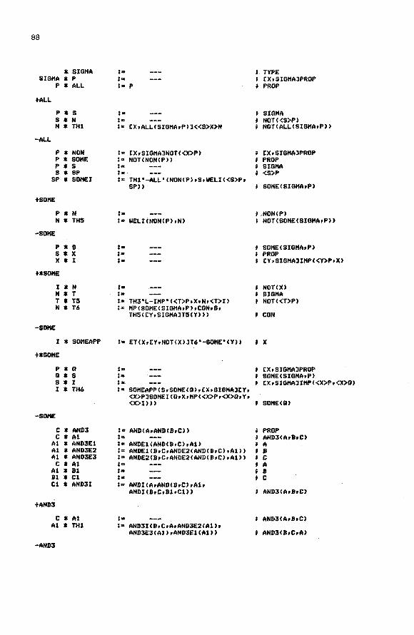
88
lk SIGHA SIGI1A lk P
-ALL
P * ALL
p * s S * N N * TH1
P * NON P * SOME p * s S * SP
SP * SOHEI
+SOME
p * N N * THS
-SOHE
p * s S * X X * I
+*SDHE
I * N N * T T * TS N * T.S
-SDHE
I * SDHEAPP
+*SOME
p * R Q * s S * I I * TH.S
-SOME
C * AND3 C * Al
Al * AND3E1 Al * AND3E2 Al * AND3E3
C * Al Al * B1 B1 * Cl Cl * AND3I
+AND3
C * Al A1 * TH1
-AND3
I• I• I= CXrALLISIGHArPll<<S>X>N
I• CXrSIGHAlNOTC<X>P) I= NOT<NONCF'l l I• I• I• TH1'-ALL'<NONCPlrSrWELIC<S>Pr
SPll
I• I• WELI(NDN(PlrNl
I• I• I• TH3'L-IHP'C<T>P•X•Nr<T>I> I• HP<SOHE<SIGHArPlrCDNrSr
TH5CCYrSIGHAlTS!Ylll
I• ET<X•CY•NOT<XlJT6'-SDHE'CYll
I• I• ; .. I• SOHEAPPCSrSOHECQlrCXtSlGHAJCYr
<X>PJSOHEICD•X•I1P<<X>Pr<X>Q,y, <X> I» l
I• AND<ArANDCB,Cl) I• I• ANDE1CAND<B•ClrA1l I= ANDE1CBrCrANDE2CANDCBrCl•A1ll I• ANDE2<B•CrANDE2CANDCBrClrAll) I• I• I• I• ANDICArAND<B•ClrAlr
ANDICBrCrBlrCll)
I• I• AND3ICBrCrArAND3E2<A1lr
AND3E3<AllrAND3E1CA1ll
TYPE CXtSIGHAJPROP PROP
SIGHA NOH<S>Pl NOTCALLCSIGHArPll
CXrSIGHAJPROP PROP SIGHA <S>P
SOHE<SIGHA•Pl
.NOtHPl NOTCSOHECSIGHArPll
SOHECSIGHArPl PROP CYtSIGHAJIHP<<Y>PrXl
NOT()() SIGHA NOn<T>Pl
CON
f X
CXrSIGHAJPROP SOHE<SIGHArPl tX•SlGHAJIHP<<X>Pr<X)Q)
SOHE(Q)
PROP AND3CAr8rCl
f A • 8 I C I A • 8
' c AND3CArBrCl
AND3<ArBrC)
AND3<BrCrAl
89
C * EC3 I= ANDJ<ECrEC<BrC)rEC<CrA)) PROP C * E I• ECJ<IIrSrC)
+EC3
E * TH1 I= ANDJE1<ECoECCBrC>•EC<CrA)r£) ECCArB> E * TH3 I= AND3E3<EC•EC<BrC)rECCCrA)r£) EC(CrA) E * TH4 := TH1'L-AND3'(ECr£C(BrC>•ECCCrA)
rE) ECJCBoCtA)
-EC3
E * Al I• A Ill * ECJ£12 I• ECElCTH1'-EC3'rA1) NOT< B) Ill * EC3E1J :· EC£2CCrArTHJ'-ECJ'oA1) NOT( C)
E * Bl I• B 81 * EC3£23 : .. EC3E12CBrCrAoTH4'-EC3'r81) NOT<C> Bl * EC3E21 I= ECJ£13CBrCrArTH4'-£C3'rB1> NOT< A>
f*EC3
c * £ I• EC<ArB) E * F I• EC<BrC> F * G I• EC<CrM G * TH6 I• AND3I<ECoECCBrC)r£CCCrA>rErFr
0) ECJCArBrC)
-EC3
+E
SIGHA * S I• SIGIIA 6 * T I• SIGHA T * IS I• PN PROP S * REF:IS I• PN ISCSrS> p * s I• SIGIIA 8 * T I• SIGHA T * SP I• f <S>P
SP * I I• ; IS(SrT> I * ISP I• PN f <T>P
SIGHA * S I• t SlGHA S * T I• f SIGHA T *· I I• J IS<SrT> I * SYHIS I• ISP<tXrSIGHAJISCXtS)rSoTr
REFIS<ShU IS<ToS) T * U I• SIGMA U * I I• xscs.n I * .J I• IS<TrU> .J * TRIS I• ISPCCXoSIGHAliSCXrUlrTrSo.Jr
SYHISCJ)) ISCSoU) U * I , .. ISCStU) I * .J I• IS<TrU) J * TRIS2 I• TRIS<SrUoTrioSYHISCTrUrJ)) Iscs.n T * N I• NOT<IS(SoT)) N * SYHNOTIS I• TH3'L-IHP'<ISCTtS>tiS<SrT>oNr
tXoiS<TrS)JSYHISCTtS•X>> NOTUS<ToS))
+NOTIS
U * N I• NOTCISCSoT>) "*1 J'!! IS<TrU) I * TH3 I• ISP(CXoSIGHAlNOTCIS<S•X>>rToUo
NrU NOT< ISCSrU)) N * I :• IS<UrT> I * TH4 I• TH3<SYHIS<UrTol)) NOTCIS(SrU))
-NOTIS
90
U * V :· SIGHA V * I •• Iscs.n I * J I• xsn.u> J * K I• IS<UoV) K * TR3IS I• TRIS<S•U•V•TRISCI•J)rk> ISCSoV) V * W I• SIGHA W * I I• xscs.n I * J I• IS<ToU) J * k I• ISUhV) K * L I• ISCVoW> L * TR4IS I= TRISCSoVoWoTR3ISCioJoK)oL> ISCSoW> P * AHONE I• CXoSIGHAJCY,SIGHAJCUo<X>PJCVr
<Y>PJISCX•Y> PROP p * ONE I= ANDCAHONE<SIGHArP>•
SOHECSIGHAoP» PROP P * Al 1 .. AHONECSIGHArP)
Al * S I• SOHECSIGHAof') S * ONEI :• ANDICAHONE<SIGHA•P>•
SOHECSIGHAoP>•AloS) DNECSIBHArP) p * 01 I• ONE<SIBHArP>
01 * IND I• PN SIGHA 01 * DNEAX I• PN <XND>P
SIGHA * TAU I• TYPE TAU * F I• CXrSIGHAJTAU
F * S I• SIGHA S * T I• SIBHA T * I I• rscs.n I * ISF := ISPCSIGHAoCXoSIGHAJISCTAU•<S>
Fo<X>F>oSoToREFISCTAUo<B>F>oi> ISCTAUo<S>Fo<T>F> TAU * F I• CXoSIGHAJTAU
F * G I• tXrBIGHAJTAU G * I I• ISCCXrBIGHAJTAUrFrG) I * S , .. SIGHA S * FISE := ISPCCXrSIGHAJTAUrCY,CX,SIGHAJ
TAUJISCTAUr<S>F•<S>Y>rFoGo REFISCTAU•<S>F>•I> ISCTAU,<S>F•<S>G>
G * I :- CXrSIGHAJISCTAUo<X>Fr<X>G> I * FISI I• PN IS<tXoSIGHAlTAUrF•G>
-E
+*E
+ST
SlBHA * SET I• PN TYPE SIGI'IA * S I• SIGHA
s * so I• SET SO * ESTI I• PN PROP P * SETOF I• PN SET I' * s I• SIGHA S * SP I• <S>P
SI' * ESTII I• PN ESTICSrSETOFCP>> S * E I• ESTICSoSETOF<P>> E * EBTIE I• PH <S>P
+EG
+LANDAU
+N
+I1
-u
+21
-21
* NAT * X X * y Y * IS Y * HIS X * S S * IN * p P * SOME P * ALL
.. 1 * sue *X
X * y y * I I * AX2
* AX3 * AX4
* s S * COND1 S * COND2
* AXS
* p P * 1P
1P * XSP XSP * X
X * S X* T1 X * y Y * YES
YES * T2 YES * T3
X * T4
X * INDUCTION * X
X * y y * H
H * I I * Tl
N * SATZ1
I• PH S• I• I• IS"E"<NATrXrY> I= NOT<IS<X•Y)) := := ESTHNAT•XrS> I= I= SOI'IE"L"CNAT•P> I= ALL "L" <HATrP) I• PH I• PH ,. I• :-I= ISFCHATrNATrSUCrXrYrl) I• PH I• PH
I• I• INU rS) I• ALL<CXrNATJIHP<IN<XrS>oiN<<X>
SUCrS))) I• PH
I• I• I• I•
loo SETDF<NATrP) I• ESTII(NATrPrlrlP> I• I• I= ESTIE<NATrPrYrYES> I= ESTIICNATrPr<Y>SUCo<T2><Y>XSP> I• <X><CYrNATJCUrlHCYoS)JT3CYrU>>
<T1><S>AX5
I• ESTIE<NATrPoXoT4"-I1") I• I• I•
I• I• <I><Y><X>AX4
I• TH3"L-II'IP"CIS<<X>SUCr<Y>SUC)r IS<X•Y>rNrCUoiS<<X>SUCr<Y>SUC>
91
TYPE HAT NAT PROP PROP SEHNAT) PROP CXrNATJPROP PROP PROP NAT tXrHATlHAT HAT HAT ISCXrY> IS<<X>SUCr<Y>SUC) CXrNATJNISC<X>SUCr1) CXtNATJCYrNATJCUoiS<<X>SUCr <Y>SUC>liSCXrY> SET<NAT> PROP
PROP CSrSET<NAT>JCUrCONDlCS)J CVrCOND2<S>JCXrNATJIN<XrS) CXrNATJPRDP <l>P CXoNATJCYr<X>PJ<<X>SUC>P HAT
SET< HAT> CONDUS> HAT IN<YoS) <Y>P IN«Y>SUCrS)
lHCXoS)
<X>P HAT HAT HISCXoY>
IS<<X>SUCr<Y>SUC) IS<XrY>
JT1"-21"<U>> f NIS<<X>SUCr<Y>SUC>
92
+23
X * PROPl I= OR<IS<XrllrSOHECtU•NATJIS<Xr <U>SUC>H PROP.
* T1 I= ORI1<IS<lrl)rSOH£CCUrNATJISC1r <U>SUC>lrREFIS<NATolll PROPHU
X * T2 I= SOHEI<NATrtUrNATJIS<<X>SUCo<U> SUClrXrREFIS<NATr<X>SUCll SOHE<tUrNATJIS<<X>SUCr<U>SUC)
)
X * TJ I= ORI2<IS<<X>SUCrllrSOHECCUrNATJ IS<<X>SUCr<U>SUCllrT2> PROP1«X>SUC)
X * T4 := INDUCTIONCtYrNATJPROP1<Y>rT1r tYrNATJtUrPROP1CY>JT3<YlrXl PROPlCXl
-23
X * H I• NIS<XrU N * SATZ3 I• ORE2<IS<XolloSOHE<CUrNATJISCXo
<U>SUC>>rT4'-23'rNl SDHE<tUrNATliS<Xo<U>SUC>l y * z I• HAT
+24
X * F I• tYrNATJHAT F * PRDPl I• ALL<CYrNATliS<<<Y>SUC>F•<<Y>f>
SUCl) PROP F * PROP2 I= AND<IS<<1>Fr<X>SUClrPROP1l PROP X * A I• tYrNATlHAT A * 8 I• tYrNATlHAT 8 * PA I• PRDP2CA)
PA * PB I• PROP2<8) PB * Y t• HAT
Y * PROP3 I= IS«Y>Ar<Y>Bl PROP P8 * T1 I= AND£1<IS<<1>Ar<X>SUClrPROP1CA)
rPA) IS<<1>Ar<X>SUC> P8 * T2 I• ANDE1<IS<<l>Br<X>SUClrPROP1C8l
rPB) IS<<l>Br<X>SUC> PB * T3 I• TRIS2CNATr<1>Ar<1>Br<X>SUCrT1r
T2l PROPJU) y * p I• PROP3CY) P * T4 I• AX2<<Y>Ar<Y>BrP) IS<<<Y>A>SUCr<<Y>B>SUC) P * T5 I= ANDE2<IS<<1>Ar<X>SUClrPROP1CAl
rPM PROP HA) p * T6 I= ANDE2<IS«l>Bo<X>SUClrPRDP1<B>
oPB> PROPUB> p * T7 I• <Y>T5 IS<<<Y>SUC>Ar<<Y>A>SUCl p * TS I• <Y>T6 IS<<<Y>SUC>Br<<Y>B>SUC) p * T9 I• TR3IS<NATr<<Y>SUC>Ar<<Y>A>SUCo
<<Y>B>SUCr<<Y>SUC>BrT7rT4r SYHIS'E'<NATr<<Y>SUC>Br<<Y>B> SUCrTS>) PROPJ<<Y>SUC>
Y *no I= INDUCTION<tZrNATJPROP3<Z>rT3r CZrNATJ[UrPROP3<ZlJT9(ZtU)rYl PRDP3(Yl
PB * T11 I• FISI<NAT•NAT•A•B•CYrNATJT10(Y) ) IS"E'CtYrNATJHATrArB)
X a AA :• CZrtYrNATJNATJtUrCYrNATJNATJ CVrPROP2<Z>lCWrPRDP2<U>JT11<Z• UrVrW) AHONE<CYrNATlNATrCZrCYrNATl
HATJPROP2<Z>> X * PROP4 I• SOHE"L"CCY,NATlNATrtZrtYrNATJ
NATJPROP2<ZH PROP * T12 I= tXrNATJREFIS<NATr<<x>SUC>SUC> PROP1UrSOC>
• T13 := ANDI<IS<<1>SUCr<l>SUC)r PROPl(lrSUC>rREFISCNATr<l>SUCl tT12) PROP2ClrSUC)
* T14 I• SOHEI<CYrNATJNATrCZrtYrNATJ NATlPROP2C1rZlrSUCrT13) PROP4U)

93
X * p :· PROP4<X> p * F I• CYrNATJNAT F * PF I= PROP2<F>
PF * G I= CYrNATJ<<Y>F>SUC CYrNATJNAT PF * y I= NAT
y * T1!5 := REFIS<NATr<Y>G> IS<<Y>Gr<<Y>F>SUC) PF * T16 1 .. ANDE1<IS<<1>Fr<X>SUC)rPROP1<F>
rPF> IS«l>Fr<X>SUC> PF * T17 := TRIS<NATr<l>Gr<<l>F>SUCr<<X>
SUC>SUCrT15<1>rAX2<<1>Fr<X> SUCrT16)) IS<<l>Gr<<X>SUC>SUC>
y * T18 := ANDE2<IS<<1>Fr<X>SUC)rPROPl<F> rPF> PROPl<F>
y * T19 I= <Y>T18 IS<<<Y>SUC>Fr<<Y>F>SUC> y * T20 I= TRIS2<NATr<<Y>SUC>Fr<Y>Gr<<Y>
F>SUCrT19rT15) IS<<<Y>SUC>Fr<Y>G> y * T21 I= TRIS<NATr<<Y>SUC>Gr<<<Y>SUC>F>
SUCr<<Y>G>SUCrTlS<<Y>SUC)r AX2<<<Y>SUC>Fr<Y>GrT20)) IS<<<Y>SUC>Gr<<Y>G>SUC)
PF * T22 I= I:YrNATJT21<Y> PROPl«X>SUCrG) PF * T23 I= ANDI<IS<<l>Gr<<X>SUC>SUC)r
PROP1<<X>SUCrG)rT17rT22) PROP2«X>SUCrG> PF * T24 I= SOMEI<CYrNATJNATr[ZrCYrNATJ
NATJPROP2<<X>SUCrZ)rGrT23) PROP4 «X>SUC) p * T2!5 I= SOMEAPP<CYrNATJNATrCZrCYrNATJ
NATJPROP2<Z>rPrPROP4<<X>SUC)r CZrCYrNATlNATl[UrPROP2<Z>l T24<ZrU)) PROP4 «X>SUC)
X * BB I= INDUCTION<CYrNATlPROP4<Y>rT14r CYrNATlCUrPROP4(Y)lT25(YrU>rX) PROP4<X>
-24
X * SATZ4 I= ONEI<CYrNATlNATrCZrCYrNATlNATl PROP2'-24'<Z>rAA'-24'rBB"-24") ONE"E"<CYrNATJNATrCZrCYrNATl
NATlAND<IS<<l>Zr<X>SUC>r ALL<CYrNATliS<<<Y>SUC>Zr<<Y> Z>SUC>>>>
X * PLUS := IND<CYrNATlNATrCZrCYrNATlNATJ PROP2"-24"<Z>rSATZ4) CYrNATlNAT
y * PL I• <Y>PLUS HAT
+*24
X * T26 I• ONEAX<CYrNATJNATrCZrCYrNATJ NATJPROP2<Z>rSATZ4> PROP2<PLUS)
-24
X * SATZ4A I• ANDEl<IS<<l>PLUSr<X>SUC)r PROP1"-24"<PLUS>rT26"-24") I IS<PL<Xrl)r<X>SUC)
+*24
X * T27 I= ANDE2<IS<<1>PLUSr<X>SUC)r PROP1<PLUS>rT26) I PROPl<PLUS)
-24
Y * SATZ4B I• <Y>T27"-24" I IS<PL<Xr<Y>SUC>r<PLlXrY>>SUC)
+*24
* T2B I= Tll<lrPLUS<l>rSUCrT26<1>rT13> I IS"E"<CYrNATlNATrPLUS<l>rSUC)
-24
X * SATZ4C I• FISE<NATrNATrPLUS<l>rSUCr T28"-24"rXl I IS(PL(lrX>r<X>SUC>

94
+*24
X * T29 I= Tll<<X>SUC•PLUSC<X>SUC>• [Y,NATJ<<Y>PLUS>SUC,T26C<X> SUC>•T23CBB•PLUS,T26)) IS'E'C[Y,NATJNAT,PLUSC<X>SUC>
,[Y,NATJ<<Y>PLUS>SUC>
-24
y * SATZ4D I= FISECNAT,NAT,PLUS<<X>SUC>• cz,NATJ<<Z>PLUS>SUC,T29'-24'• Y> ISCPL<<X>SUC•Y>r<PL<X•Y>>SUC)
X * SATZ4E I= SYHISCNAT,PL<X•l>•<X>SUC• SATZ4A> ISC<X>SUC,PL<X•l))
y * SATZ4F I= SYHISCNAT,PL<X•<Y>SUC>•<PL <X•Y>>SUC,SATZ4B> IS<<PLCXrY>>SUC•PL<X•<Y>SUC))
X * SATZ4G I= SYHISCNAT,PL<l•X>•<X>SUC• SATZ4C> IS<<X>SUC,PL<l•X>>
z * I I= IS<X•Y> I * ISPL1 := ISF<NAT•NAT•CU,NATJPL<U•Z>•X•
y,J) ISCPL<X•Z>•PL<Y•Z>> I * ISPL2 I= ISFCNAT,NAT,CU,NATJPL<Z•U>•X•
Y•I> ISCPL<Z•X>•PL<Z•Y>>
+2:5
z * PROP1 I= ISCPLCPL<X•Y>•Z>•PL<X•PL<Y•Z>> ) f PROP
y * T1 I= TR3IS<NAT,PL<PL<X•Y>•l>•<PL <X•Y>>SUC,PLCX,<Y>SUC), PL<X,PL(Y,l)),SATZ4ACPL<X•Y>>• SATZ4F,ISPL2C<Y>SUC,PL<Y•1>•X• SATZ4E ( Y> )) PROP1<1)
z * p I= PROP1<Z> p * T2 I= AX2CPL<PL<X•Y>,z>,PL(X,PL(Y,z>
>•P> IS<<PL<PL<X•Y>•Z>>SUC•<PL <X•PL<Y•Z>>>SUC)
p * T3 I= TR4ISCNAT,PLCPL<X•Y>•<Z>SUC>• <PL<PL<X•Y>•Z>>SUC,<PL<X•PL <Y•Z>>>SUC,PL<X•<PL<Y•Z>>SUC>• PL<X,PL<Y•<Z>SUC>>• SATZ4B<PL<X•Y>,z>,T2• SATZ4F(X,PL<Y•Z>>• ISPL2<<PL<Y•Z>>SUC,PL<Y•<Z> SUC>•X•SATZ4F<Y•Z>>> f PROP1 «Z>SUC)
-2:5
Z * SATZ:S := INDUCTION<CU,NATJPROP1'-2:S'CU) •T1'-25',[U,NATJCV•PROP1'-2:S' CU>JT3'-25'CU,V>•Z> ISCPLCPL<X•Y>•Z>•PL<X•PL(Y,Z)
))
Z * ASSPL1 I= SATZ:S IS<PLCPLCX,Y>•Z>•PLCX,PLCY•Z> ))
+26
Y * PROPl I= ISCPL<X•Y>•PL<Y•X>> PROP y * T1 I= SATZ4ACY> IS<PLCY•l>•<Y>SUC) Y * T2 la SATZ4CCY> IS<PL<1•Y>•<Y>SUC> y * T3 I= TRIS2<NAT•PL<l•Y>•PL<Y•l>•<Y>
suc.T2•T1> PROP!ChY> y * p I• PROP1CX•Y> p * T4 I= TRIS<NAT•<PL<X•Y>>SUC,<PL<Y•X)
>SUC,PL<Y•<X>SUC>•AX2CPL<X•Y>• PL<Y•X),p),SATZ4F<Y•X>> ISC<PL<X•Y>>SUC,PLCY•<X>SUC))
p * T:S I= SATZ4D ISCPLC<X>SUC•Y>•<PL<X•Y>>SUC) P * T6 I• TRIS(NAT•PL<<X>SUC•Y>•<PL<X•Y>
>SUC,PL<Y•<X>SUC>•T5,T4) PROPl «X>SUC' Y>
-26
Y * SATZ6 I= INDUCTION<CZ•NATlPROP1'-26'CZr Y>•T3'-26',[Z,NATJ [U,PR0Pl'-26'<Z•Y>JT6'-26'<Z• v.u>ox> IS<PL<X•Y>•PL<Y•X>>
Y * COHPL I= SATZ6 IS<PL<X•Y>•PL<Y•X>>

+27
-27
+29
Y * PROP1 X * T1 X * 12
y * p P * T3 P * T4
Y * SATZ7
Z * DIFFPROP
y * I y * II Y * III Y * OHE1
OH£1 * U u * T1
U * T2
ONE1 * T3
Y * T4 ONEl * T5
y * 16 Y * TW01
TW01 * THR££1 THREE1 * U
U *DU DU * V V* lW
DV * T6A
T.HREE1 * T9
TW01 * T10 Y *TU y * 11
-29
Y * SATZ9B
Y * MORE Y * LESS Y * SATZ10B
y * " M * SATZ11 Y * MOREIS Y * LESSIS y * M H * SATZ13
I• HIS< Y, PL <X, Y)) I• SYHNOTIS<NAT•<X>SUCr1•<X>AX3> I= TH4'E-NOTIS'<NATo1r<X>SUCr
PL<Xr11rT1rSATZ4A> I• I• SATZl<YrPLCXrYirP) I= TH4'E-NOTIS'<NATr<Y>SUCr<PL
<XrYI>SUCrPL<X•<Y>SUCirT3r SATZ4B>
le INDUCTION([ZrNATJPROP1'-27'(Z) rT2'-27'rCZrNATJ[UrPROP1'-27' <Z>JT4'-27'<ZrUirY>
I= IS(XrPL<YrZ))
I• IS<X•Y> I• SOHE<CUrNATJDIFFPROP<XrY•U)) I• SOKECCVrNATJDIFFPROPCYrXrV)) I• I• I• TRIS<NATrPLCUrXIrPLCXrU)r
PL<YrUirCOMPL<U•X>• ISPL1CUtONE11)
I• TH3'E-NOTIS'CNATtXrPL(UtXIo PL<YrUirSATZ7CUrXIrT11
I• TH5'L-SOME'(NATrCU•NATJ DIFFPROP<Uio[UrNATJT2<U>>
I= TH1'L-EC,• U, IZ.tZ• IlT3<Z>) , .. T3CYtXrSYMIS<NATrXrY•ONE11) I• TH2'L-EC'<IIItirCZrllT5(Z)) I• I• I• I• I• I• I• TR4ISCNATrXrPLCYtUirPL<PL<X•V>
rUirPLCXrPL<VrUIItPL<PL<VrUI• XlrDUriSPL1(Y,PL<XrVIrU,DVIt ASSPLl(XrVtUitCOMPLCXtPL<VrU)) )
I= KPCISCXtPL<PL<V•U>•X)),CONt T6ArSATZ7<PL<VrU>•X>>
l= SOHEAPPCNATrCVtNATJDIFFPROP<Y• XrV>•THREE1rCONrCVrNATJ CDVrDIFFPROPCYrXrV>JT7CVtDU)) ·- SOMEAPP<NATrCUrNATJDlFFPROP!U) 41':
rTWOlrCONrCUrNATJtDUtDIFFPROP (U)JTSCUrDU))
:= CZtiUJT9(Z) :- TH1"L-E~"<IIriii•CZtiiJT10(Z))
:- TH6"L-EC3"CiriiriiirT4rT11tT6>
t• A"-29 1
t• SOHECCU.NATJDIFFPROP<X•Y•U>> t= SOHE<CV,NATJDIFFPROP<Y•X•V>> ; .. SATZ9B
•• t• " I= ORCMOREoiSCXrY)) t= ORCLESStiS<XrY>>
t= TH9'L-OR'<MOREtiS<XrY>r LESS<Y•X>riSCYtX)tHrCZ•HDREJ SATZ11<ZirCZriSCXtYIJ SYHIS<NATrXrYrZ))
95
PROP N1SC lt<X>SUC)
PROPHU PROPHY) NIS<<Y>SUCr<PLCXrY))SUC)
PROPH <Y>SUC)
NISCYrPL<X•Y» PROP
I PROP f PROP I PROP f I I NIIT
ISCPLCUrXIrPL<YrUI)
NISCXrPL<YrU»
NDT<IU EC<IriU NOT<IIU EC<Uhl> II Ill NAT DIFFPROP<X•Y•U> NAT DIFFPROP<Y•X•V>
ISCXtPL<PL<VrUitX))
CON
CON
CON NOT<UI> EC<IX.III> EC3'<IriioUJ>
EC3'<IS(XoYirSOHE<CUrNATl DIFFPROP<X•YrU>>•SOHE<CV•NATl DIFFPROPCYoXtV))) PROP PROP EC3<IS<X•Y>•HORE<X•Y)r LESSCXtY>) KOREO<•Y> LESS(Y•X> PROP PROP I'IOREISCXoY>
I LESSISCYrX>

96
Z * I I• IS<XrY> I * M , .. MORE<XrZ) M * ISMOR£1 I= ISP<NATrCUrNATJMORE<UrZ>rXrYr
MrU HORE<YrZ) I *M I• MOREISCXrZ) M * ISHOREIS1 I= ISPCNAT,CUrNATJMOREIS<U•Z>•X•
y '"'I) MOREIS(Y,z) I * M I• HOREISCZ,X) M * ISHOREIS2 I= ISPCNATrCUrNATJMOREISCZrU>rXr
Yrltri) HOREISCZ•Y> y * I I• IS<X•Y> I * KOREISI2 I• ORI2CtiORECXrY>, I'SCXrY>,!) HOREISCXrY> y * 11 I• tiORE<X•Y> 11 * HOREISI1 I= GRilCHORE<X•Y>riSCXrYirH> ; HOREIS<XrY> z '* u I• ; NAT U * I I• ; xscx.n I * J I• p IS<ZrU> J * H I• f MOREISCXrZ> H * ISHOREIS12 I• ISHOREIS2<Z•U•YrJr
ISHOREISl<X•Y•ZrirM)) HOREIS(Y,U) y * H I• HORECXtY> M * SATZ10G I• TH3"L-OR"CLESSCXrY)riS<X•Y)t
EC3E23CIS<X•Y>rti0R£(X•Y>t LESSCXrY>•SATZ10BrH)r EC3E21CISCXrY>rHDR£(XrY>• LESSCXrY)rSATZlOBrH>> NOTCLESSISCXtY)>
y * SATZ18 := SOHEICNATrCUtNATl DIFFPROPCPLCXrY>rXrU>rYr REFISCNATrPLCXrYI>> HORE<PLCXrY>tX)
Z * M I= ttORECXtY>
+319
M * U I• HAT U * DU I= DIFFPROP(U)
DU * T1 I= TRISCNATtXrPL(Y,U>rPLCUrY>rDUt COHPLCYrU» ISCXrPL(UrY>)
DU * T2 I• TR3ISCNATrPLCXrZ>•PL<PLCUrY>t Z>rPLCUrPLCYrZ>>rPL<PLCYrZ>rU) riSPLlCXrPLCUrY>rZrTl)r ASSPLl(U,YrZ)rCOHPL<UrPLCYoZ)) ) IS<PL<XrZ>rPLCPL<YrZ>oU))
DU * T3 I• SOHEI<NATrCVrNATl DIFFPROPCPLCXrZ)rPLCYrZ>rV)tUo T2> HORECPL<XrZ)rPLCYtZ))
-319
H * SATZ19A I• SOHEAPP<NATrCUrNATlDIFFPROPCU) •tlrHORE<PLCXrZ>•PL<Y•Z>>• CU,NATJ[V,DIFFPROPCU)l TJ"-319" cu,v> > HORE<PLCXrZ>rPLCYrZ))
z * M I• HOREISO(tY>
+*319
H I N I• HORECXrY> H * T4 I• HOREISil<PL<XtZ)rPL<Y•Z>•
SATZ19A(N)) HOREISCPL<X•Z>rPL<Y•Z>> H * I :· ISCXrY) J * T5 , .. HOREISI2<PLCXrZ>rPL<YrZ)r
ISPLHXtYrZri>) HOREISCPLCXrZ>rPL<Y•Z>>
-319
M * SATZ19L I= ORAPP<MORE<XrY>•ISCX•Y), ttOREISCPL<XrZ>rPL<YrZ>>•Mt CUrMORECX•Y>lT4"-319•(U),[U,IS (XrY)JT5"-319"<U>) HOREIS<PL<XrZ>•PLCYtZ))
H * SATZ19H t• ISHOREIS12CPL<X•Z>rPL(ZrX), PL<V,z>,PL<Z•Y>rCOHPL(XrZ>• COMPL(YrZ>rSATZ19L> ttOREIS<PL<Z•X>tPL<Z•Y>>

97
+324
X * H ,. NIS<X•U
N * U , .. NAT U * I t• IS<X•<U>SUC) I * T1 I= TRISCNAT•X•<U>SUC,PLCl•U>•l•
SATZ4G<Ul) IS<X•PL<l•U)) I * T2 I• ISHORElCPLCl•U>•X•l•
SYHISCNAT•X•PLCl•U>•Tl), SATZlSC 1 ,U) > 11DRECXrU
H * T3 , ... SOHEAP~CNAT•CU•NATJIS<X•<U>
SUC>•SATZ3<X•N>•MORE<X•l>• tU•NATJCV,ISCXr<U>SUClJT2CUrV) ) I HDRECX,U
-324
X * SATZ24 I• TH2'L-OR'CHORECXrl>•ISCXrllr CU,HIS<X•l>JT3'-324'CU)) MOREISCX• U
X * SATZ24A I• SATZ13CX•l•SATZ24) LESS IS< 1 ,)() y * 11 I= MORECYrX)
+325
" * u I• NAT
U * DU !• DIFFPROP<Y•X•U> nu * n I• SATZ19HCUrl•XrSATZ24CU)) MOREISCPLCXrU),PLCXrl)) DU * T2 I• ISHOREIS1CPLCXrUlrYrPLCXtl)t
SYHISCHATrY•PL<X•UlrDU>rTll HOREISCYrPLCX•ll)
-325
H * SATZ25 I• SOHEAPPCNATtf.UrNATlDIFFPROPCY• XrU>rH•HOREISCY,PL<X•l))r CUrNATJCVrDlFFPROPCYrXrUl.l T2'-325' CUr V)) HOREIS<Y•PLCXr1))
y * L I• --- LESSCYtX) L * SATZ25B I• SATZ13CXtPL<Y•llrSATZ25CY•X•L>
) LESSISCPL<Y•l)rX) * p I• CXrNATlPROP
P * N ,. NAT
+327
N * M ,. HAT H * LBPROP := IHPC<H>PrLESSIS<N•H>l PROP
-327
N * LB I• ALLCCXrNATJLBPROP'-327'CXl) PROP N * HIN !• ANDCLBr<N>P> PROP p * s I• SOMECP>
+*327
S * N I• NAT N * T1 I• CXr<N>PJSATZ24A<N> LBPROPCloN) S * T2 I= [X,NATJT1CX> LBUl S * L , .. CXtNATlLBCX> L * y I• HAT Y * YP I• <V>P
YP * T3 , .. SATZ18CYtU HORE<PLCYtl),Y) YP * T4 I• SATZ10GCPLCY•l>•Y•T3) NOTCLESSlSCPL<Y•1>•Y)) yp * Tl5 ,. TH4•L-IKP"C<Y>P•LESSISCPLCYr1)
rYhYP•T4l NOTCLBPROPCPLCYr1)rY)) YP * T6 :• THi'L-ALL'CNATr[XtNATl
LBPROPCPLCYr1lrX)rYrT5> NOTCL~CPL<Yr1))) yp * T7 ,. KPCLB<PLCYr1)),CONr<PLCYr1l>L•
T6> CON L * re , .. SOHEAPPCNATrPrSrCONrCX•NATJCY•
<X>PJT7<XrY» CON

98
S * N
11 * H H * L L * T9
L * T10
L * Tll
N * T12
s * T13
S * H 11 *A A* T14
A* T15
A * NHP NHP * N
N * NP NP * T16 NP * T17
NP * TlB
NP * T19 NHP * T20 NHP * T21
A * T22 A * T23
-327
S * SATZ27
-N
-LANDAU
-EQ
-sr -E
-L
I"'
I• I• I• <H>H
I• ET!LB!PL<Hrl)), TH3•L-AND•(L8C/1)r NDTCLBCPL<Hr1)))rT9rL))
I= lSPCNATrtXrNATJLB!X)rPL<Hrl)r <H>SUCrT10rSATZ4ACHll
I• CXrNATJINDUCTIDNCCYrNATJLB<Y>r T2rCYrNATJCZrLB!YllT11CY•Z>•X>
I• CXrNONCNAToCXrNATJAND<LB<X>• NOTCLBCPL<X•ll))l)JTSCT12CXll
I• I• I= ANDE1!LBCI1)rNOT<LB<PLCI1rl)))r
A> I• ANDE2CLBC/1),N0T(LBCPLCH,1>>>•
Al I• I• I• I= HP<<N>P•LESSISCHrNlrNPr<N>T14) I= TH3'L-IHP"<ISCI1rNlr<H>PrNHPr
CXriSCHrNlliSP<NATrPrNrHrNPo SYHISCNATrH•NrX)))
I= ORE1CLESSCI1rNlrJSCHrN>•T16o T17)
I= SATZ25BCNrH•Tl8l I= CXrNATJCYr<X>PJT19CXoY> I• HP<LBCPLCHrlll•CDNoT20rT15l I• ET<<H>PrCX•NDTC<H>P)JT21CXll I= ANDI<LB<tt> r<H>P• T14r T22)
I= TH6'L-SOI1E'<NAT•tXrNATJ AND!LB!XlrNOTCLB!PL<X•ll)))r tXrNATJHIN<X>•T13'-327'• CX•NATJtYrAND!LBCX)r NOT!LBCPL(Xrl))))JT23"-327"(Xr
NONCNATrCXrNATlAHD<LB<X>r NOTCLBCPL!Xrll)l)) NAT LBC/1) NOTCAND<LBC/1)rNOT<LBCPLCI1o1)) )))
LBCPL(/1,1))
LB«H>SUC)
CXrNATJLBCXl
SOHE<CXrNATJAND<LBCX>r NOT<LB<PLCXrl))))) HAT AND!LBCH),N()TCLBCPL<H•l))))
LBUO
NOTCLBCPL<H•l))) NOT«H>P) NAT <N>P LESSJSCHoN)
NOTUSCHrN))
LESS!Hrlll LESSISCPL!HrllrNl LB!PL<thll) CON <H>P ltiHCH>
Y)) f SOHE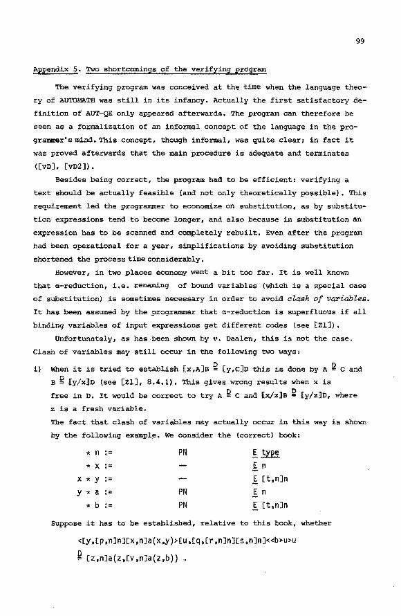
99
Appendix s. Two shortcomings of the verifying proqram
The verifying program was conceived at the time when the language theo
ry of AUTOMATH was still in its infancy. Actually the first satisfactory de
finition of AUT-QE only appeared afterwards. The program can therefore be
seen as a formalization of an informal concept of the language in the pro
grammer's mind. This concept, though informal, was quite clear; in fact it
was proved afterwards that the main procedure is adequate and terminates
([vD], [vD2]).
Besides being correct, the program had to be efficient: verifying a
text should be actually feasible (and not only theoretically possible). This
requirement led the programmer to economize on substitution, as by substitu
tion expressions tend to become longer, and also because in substitution an
expression has to be scanned and completely rebuilt. Even after the program
had been operational for a year, simplifications by avoiding substitution
shortened the process time considerably.
However, in two places economy went a bit too far. It is well known
that a-reduction, i.e. renaming of bound variables (which is a special case
of substitution) is sometimes necessary in order to avoid otash of v~iables. It has been assumed by the programmer that a-reduction is superfluous if all
binding variables of input expressions get different codes (see [Zl]).
Unfortunately, as has been shown by v. Daalen, this is not the case.
Clash of variables may still occur in the following two ways:
i) When it is tried to establish [x,A]B ~ [y,C]D this is done by A ~ c and
B ~ [y/x]D (see [Zl], 8.4.1). This gives wrong results when xis D D free in D. It would be correct to try A • C and [x/z)B = [y/z]D, where
z is a fresh variable.
The fact that clash of variables may actually occur in this way is shown
by the following exampl~. We consider the (correct) book:
* n
* X
X * y
y * a
* b
.-
.-:=
.-
.-
PN
PN
PN
~~ E n
~ [t,nJn E n ~ [t,nJn
Suppose it has to be established, relative to this book, whether
<[y,[p,nJnJ[x,nJa(x,y)>[u,[q,[r,nJnJ[s,nJnJ<<b~u>u
0 = [z,nJa(z,[v,nJa(z,b)) •

100
It is easily seen that both expressions are correct, and that the first
expression reduces by ~-reductions to
[x,nJa(x,[x,nJa(x,b))
where, as it should be, in the subexpression [x,n]a(x,b) the second x
is bound. Hence the expressions are not definitionally equal. The pro
gram will not discover this, because it will proceed to check
[x,nJa(x,[x,nJa(x,b)) ~ rx.nJa(x.[v,nJa(x,b}}
and then a= a x R x and [x,nJa(x.b} R [x,nJa(x,b). ii) The claim (in [Zl], 5.1) that by ~-reductions on expressions with dis
tinct binding variables eventually no clash of variables can arise is
not justified, as we show by another example: Consider the following
(correct) book:
Now
* n
* X
X * y
y * a
* b
.-:=
.-
.-:=
PN
PN
PN
<[z.[i,n][j.n]nJ[y,nJ(x,nJa(<x>z,y}> [u,[k,[l,nJ[m.nJnJ[p,nJ[q,nJnJ<<b>u>u
reduces by a-reductions to
[y,nJ[x,nJa(<x>[y,nJ[x.nJa(<x>b.y),y) (1} (2) (3)
I~ I [t,n]n E n
E n
I [t,nJ[u,nJn
If we reduce this further, the x indicated by (2), which is bound by
the abstraction indicated by (1), will be bound by the abstraction in
dicated by (3) 1 since the expression reduces (in the verifying program)
to
[y,nJrx.nJa([x,nJa(<x>b,x),y) (1) (3) (2)
while it should reduce to
[y,nJ(x.nJa(Cv,nJa(<v>b,x),y} (1) (3) (2)
(where vis a new variable).

101
Appendix 6. Example of a text in AUT-68
* PROP := PN I~ * A .- E PROP
A * 1- .- PN I~
* s .- I~ s * p .- I Ex,SJPROP P * ALL .- PN E PROP p * V := ALL E PROP P * a := E S a * u .- I 1-(V(P)) u * ALLe := PN I 1-{<a>P) u * ve := ALLe E 1-( <a>P) p * u .- I Ex.SJI-(<x>P) u * ALLi := PN I 1-{V(P)) u * Vi .- ALLi I f-(V(P))
p * B .- E PROP B * A+B .- ALL(f-{A),[x,f-(A)JB) E PROP B * u .- I 1-{A+B) U * V .- I 1-(A) u * -+e := ALLe(r(A),Ex,r(A}lB,v,u) I 1-(B} B * u .- I [x,f-(A)JI-(B) u * +i .- ALLi(r(A),[x,f-(A)JB,u) I f-(A+B)
* .L .- ALL(PROP,Cx,PROPJx) E PROP A * u := I 1-{.L) u * .1e := ALLe(PROP,[x,PROP]x,A,u) I 1-(A}
A*r .- A+.L E PROP B * AvB := ALL(PROP.Ex,PROPJ((A+x)+((B+x)+x))) E PROP B * X .- E PROP X * u := I 1-(AVB) U * V .- I [x,f-(A)Jf-(X) V * W .- I [x,f-(B)Jf-(X) w * ve := +e(B+X,X,+e(A+X,(B+X)+X,
ALLe(PROP,[x,PROPJ((A+x)+((B+x)+x)), X,u),+i(A.X,v)),+i(B,X,w)) I 1-(X)
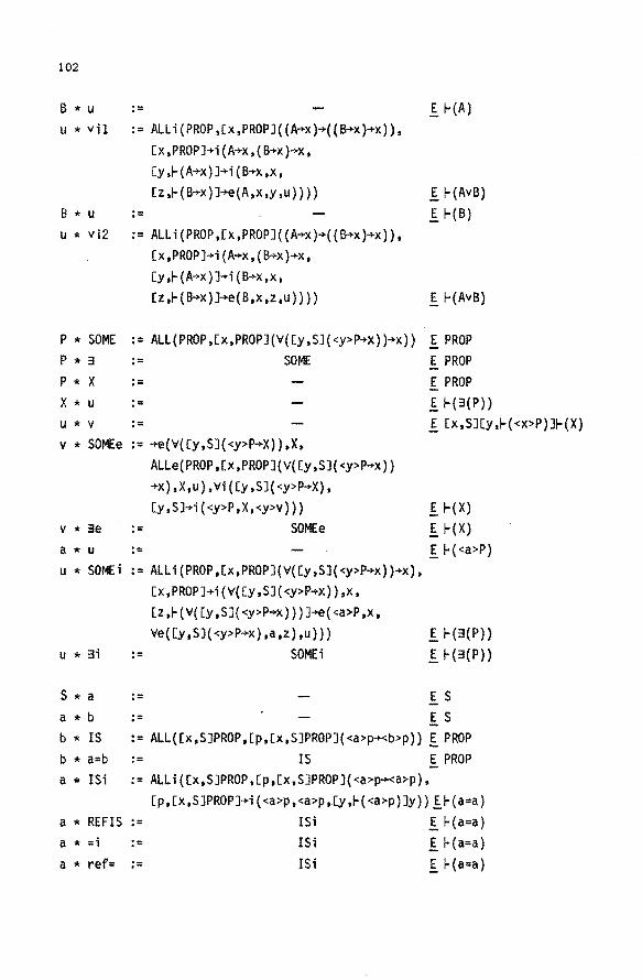
102
B * u :=
u * vil := ALLi(PROP,[x,PROPJ((A~x)~((B+x)~x)),
[x,PROPJ~i(A~x,(B+x)~x,
Cy,r(A~x}J~i(B+x,x,
[z,r(B+x)J~(A,x,y,u}}})
B * u
u * vi2 := ALLi{PROP,[x,PROPJ({A~x)~({B+x)~x)), [x,PROPJ~i(A~x,(B+x)~x,
[y,r{A~x)J~i(B~x,x,
[z,r{B+x)J~e(B,x,z,u))))
I 1-(A)
I 1-{AvB) I HB)
I 1-{AvB)
P * SOME := ALL(PROP,[x,PROPJ(V([y,SJ(<y>P~x))~x)) I PROP p * 3
p * X
X * u U * V
:=
:=
SOME
v * SOMEe := ~(V([y,SJ{<y>P~X)),X,
ALLe(PROP,[x,PROPJ(V([y,SJ{<y>P~x)}
~x),X,u),Vi([y,SJ(<y>P~X),
[y,SJ~i(<y>P,X,<y>v}})
v * 3e := SOMEe
I PROP E PROP I I-(3(P}}
I cx,SJ[y,r(<x>P)Jr(X)
I r(x) I 1-{X}
a* u .- IH<a>P) u * SOMEi := ALLi(PROP,[x,PROPJ(V([y,SJ(<y>P~x))~x),
[x,PROPJ+i(V([y,SJ{<y>P~x)),x,
[z,r(V([y,SJ{<y>P~x)))J~(<a>P,x,
u * 3i
S * a
a * b
·.-:=
ve{[y,SJ{<y>P~x),a,z),u)))
SOMEi I I-{3{P))
E I-(3(P))
E S
E S
b * IS := ALL([x,SJPROP,[p,[x,SJPROPJ(<a>p~b>p)) I PROP b * a=b := IS E PROP a * ISi := ALLi([x,SJPROP,[p,[x,SJPROPJ(<a>p~a>p),
[p, [x,SJPROPJ+i ( <a>p ,<a>p ,.[y ,I-( <a>p) Jy}} IH a=a} a * REFIS := ISi I r{a=a) a * =i .- ISi I 1-(a=a) a * ref= .- ISi I r(a=a)

p * a
a * b
b * u
U * V
.-
:=
.-v * ISe := -+e(<a>P,<b>P,ALLe([x,SJPROP,
[p,[x,SJPROPJ(<a>p+<b>p),P,u),v) v * SUBST.PRED .- ISe v * =e
S * a
a * b
b * u
u * SYM. IS u * sym=
b * c e * u U * V
v * TR. IS v * tr=
S * T T * f
f *a
a * b
b * u
:= I Se
:=
:= :=
:= =e(Ex,SJ(x=a).a,b,u,=i(a)) := SYM. IS :=
:= :=
:= =e([x,SJ(a=x),b.c.v,u) := TR.IS
:= •(a=b)
.-:=
:=
:=
u * SUBST.FN := =e([x,SJIS(T,<a>fo<X>f), a,b.u,ISi(T,<a>f))
+N
* nat := PN
* p := p * V := ALL(nat,P} p * n .-n * u ·-.-u * ve := Alle(nat,P,n,u)
E S
E S
I 1-(a=b) f 1-(<a>P)
f 1-{<b>P) f 1-{ <b>P) f 1-(<b>P)
IS E S
I 1-{a=b) f 1-{b=a) I 1-(b=a) E S
I 1-(a=b) I Hb=c) f 1-{a=c) I 1-{a=c)
E PROP
I~ I [x,SJT f.S E S
f 1-(a=b)
103
f 1-(IS(T,<a>f,<b>f))
f~ f [x,natJPROP I PROP E nat f 1-(V(P))
I t-(<n>P)

104
p * u .- I Ex.natJr(<x>P) U * Vi := ALLi(nat,P,u) I 1-(V(P))
p * 3 := SOME(nat,P) I PROP p * X := E PROP X * u :• .[ H3(P)) U * V := .[ Ex,natJEy.r(<X>P)Jr(X) v * 3e .- SOMEe(nat,P,X,u,v) E 1-(X) n * u .- I f-(<n>P) u * 3i := SOMEi(nat,P.n,u) .[ I-(3(P))
* n := .[ nat n * m := .[ nat m* n=m := IS(nat,n,m) .[ PROP m * njlm := •{n=m) E PROP
n * ref= := REF. IS(nat,n) .[ 1-(n=n} m * u .- 1 1-(n=m) u * sym= .- SYM.IS(nat,n,m,u) .[ 1-(m=n) m * 1 ·- 1 nat .-l * u := 1 1-(n=m) U * V := g_ f-(m=l) v * tr= :• TR.IS{nat,n,m,l,u,v) E 1-{ n=l)
p * n ·- f nat .-n *m := E nat m * u := f f-(n=m) U * V := .[ 1-{<n>P) V* subst.pred := SUBST.PRED(nat,P,n,m,u.v) E 1-{<m>P)
s * f := f [x,natJS f * n := E nat n *m := E nat m* u .- .[ 1-(n=m) u * subst.fn .- SUBST.FN(nat,S,f.n,m,u), 1 f-{IS(S,<n>f,<m>f))
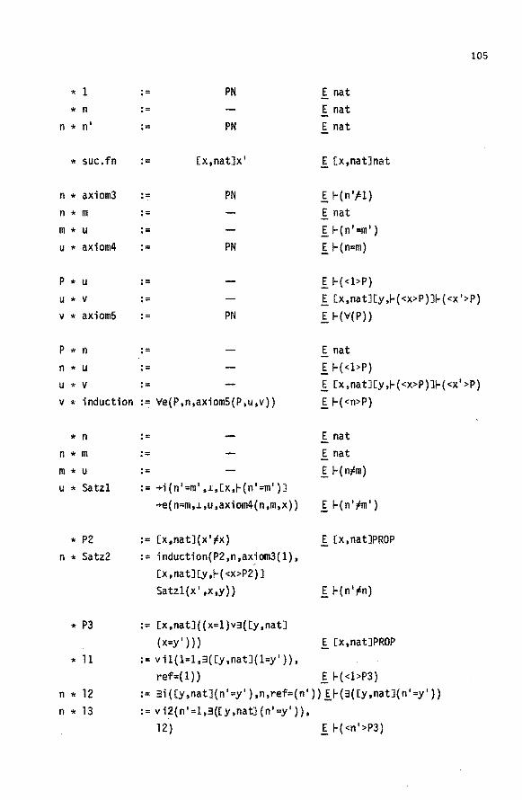
* 1
* n n * n'
* suc.fn
n * axiom3 n * m m * u u * axiom4
p * u u * V
V * axiomS
P * n
.- PN :=
.- PN
.- [x,natJx'
:= PN :=
.-
.- PN
.-
.-:= PN
:=
~ nat E nat E nat
~ [x,natJnat
.[ 1-{n'Fl) E nat ~ Hn'=m') ~ 1-{n=m)
~ 1-{<l>P)
105
~ [x,natJ[y,l-(<x>P)JI-(<x'>P) ~ 1-{V(P))
E nat n * u .- ~ 1-{<l>P) U * V ,- ~ [x,natJ[y,l-(<x>P)JI-{<x'>P)
~ 1-{ <n>P) v * induction := Ve(P,n,axiomS(P,u,v))
* n n * m m * u u * Satzl
* P2 n * Satz2
* P3
*11
n * 12
n * 13
·.-
:= := +i(n'=m·.~.[x,r(n'=m')J
+e(n=m.~,u,axiom4(n,m,x))
:= [x,natJ(x'FX) := induction{P2,n,axiom3(1),
[x,natJ[y,r(<x>P2)J Satzl{x' ,x,y))
:= [x,natJ((x=l)v3([y,natJ (x=y' )))
:= vil(l=l,3([y,natJ(l=y' )),
E nat E nat ~ l-{n1m)
~ l-(n'1m')
~ [x,natJPROP
E 1-(n'jEn)
~ [x,natJPROP
ref=(l)) ~ l-(<l>P3) := 3i ([y,natJ(n'=y') ,n,ref=(n')) ~l-(3([y,natJ(n'=y'}} := v i2(n'=l,3([y,nat] (n'=y')),
12) ~ l-(<n'>P3}

106
n * 14
n * u
:= induction{P3,n,ll,[x,nat] [y,~{<X>P3]13{x})
.-u * Satz3 := ve(n=l,3([y,natJ(n=y'}},
3([y,natJ(n=y'}},l4,[x,~(n=l)J~e
{3([y ,natJ( n=y')) ,-+e( n=l,~,u ,x)), [x,~(3{[y,natJ(n=y'}))Jx)
f. 1- ( <.n>P3) .[ r(n;!l)
f l-(3([y,natJ(n=y')}}

107
Appendix 7. Excerpt for "Satz 1", "Satz 2" and "Satz 3".
LAYOUT FROH FILE EXCERPTOUTPUT/SATZ1EN2EN3 JANUARY 25r 1977
+t.
* A =· PROP A * B , .. PROP B * IHP , .. tXrAlB PROP B * C t• ; PROP C * I ,. f IHP<ArB) I * J I• • IHPCBrC) J * TRIHP I= CXrAl«X>I>J ' IHPCArC> * CON I= PN ' PROP A * NOT , .. IHPCCON) f PROP A * WEL I• NOTCNOTCA)) f PROP A * A1 , .. ' A
A1 * WELI I= CXrNOT<A>l<A1>X ' WELCA> A * W , .. f WEt.< A> W * ET I• PN ' A A * Cl , .. ' CON
Cl * CONE I• ET<CXrNOT<A>lCl) • A
tiHP
B * N ,. NOT< A> N * TH2 I• TRIHPCCONrBrNrtXrCONlCONEIBrX>
) f IHPCAriU B * N ,. f NOTCB> N * I I• f IHPCArB> I * TH3 I• TRlttPCCONrirN> f NOT<A>
-IHP
B * OR I• IHPCNOT<A>rB> PROP 8 * A1 , .. A
At * ORU , .. TH2"-IHP"CNOTCA>•BrWELICA1)) OR(ihB) 8 * 81 ,. B
81 * ORI2 I• CX•NOHA>l81 ORCAriU B * 0 =· OR<ArJ) 0 * N I• NOT( A> N * ORE2 I• <N>O 8 * SIGHA I• TYPE
SIGMA * P I• tXrSIGHAlPROP P *ALL ,_ p PROP
+ALL
p * s I• SIGMA S * N I• NOT<<S>P> N * TH1 I= CXrALL<SIGHA•P>l<<S>X>N NOT<ALL<SIGHArP)>
-ALL
P & NON ; .. CXrSIGHAlNOT<<X>P> CXrSIGHAlPROP P * SOME I• NOHNOIHP)) PROP p * s I• SIGMA S * BP ,. <S>P
BP * SOI'IEI I• TH1"-ALL"<NON<P>rSrWELII<S>Pr SP)) SOHECSIGHArP)
+E
SIGHA * S I• SIGHA S & T I• SIGMA T * IS =· PN PROP S * REFIS I• PN ISCSrS>
-E

108
+*E
+ST
SIGHA I SET SIGtiA * S
s * so SO * ESTI P * SETOF p * s S * SP
SP * ESTII S * E E * ESTIE
+EQ
+LAHDAU
+N
+U
-u
+21
-21
I HAT * X
X * y Y * IS Y * NXS X * S SI IN
* p P I SOHE P *ALL
* 1 *sue * AX3 * AX4
* s S * COND1 S I COND2
I AXS
* p P * 1P
1P * XSP XSP *X
X * S X * T1 X I y Y * YES
YES * T2 YES * T3
X * T4
X I INDUCTION * X
X * y y * N
N I l I * T1
N * SATZ1
I• PH I• I• I• PN I• PN I• :• , .. PN I• I• PN
I• PN :• : .. I• IS"E"<NATrXrY) la NOTUSCXrY)) I• I= ESTI<NATrXrS) : .. I• SOtiE"L"CNATrP) I= ALL"L"CNATrP) I= PN := PH t= PN I• PH
I• ;a IN<lrS) := ALLCCXrNATJitiPCINCXrS)riN<<X>
SUCrS>>> I= PH
I= SETOFCNATrP) t• ESTIICNATrPololP) I• I• I• ESTIECNAT•P•YoYES> I= ESTII<NATrPr<Y>SUCtCT2><Y>XSP> I• <X><CYrNATJCU•INCVoS)JT3CYtUl>
<Tl><S>AX5
I= ESTIE<NAT•PrX•T4"-I1") I• I• I•
I• :• <I><Y><X>AX4
I= TH3"L~lHP"CISCCX>SUCr<Y>SUC)r IS<X•YlrN•CU•ISCCX>SUC•<Y>SUC> JT1"-21' CU))
TYPE SIGHA SET PROP SET SIGHA <S>P ESTICSrSETOFCP)) ESTICSrSETOF<P>> <S>P
' TYPE I MAT f HAT I PROP I PROP I SETCHAT> I PROP f CXoHATJPROP f PROP ' PROP f NAT I CXoHATJNAT I CXrNATJNISC<X>SUCr1) f CXrNATJCYrNATJCUriS<<X>SUCr
CY:>SUC>JISCXrY> I SET<NAT> I PROP
PROP CStSETCNAT>JCUrCOND1CS)J CVtCOND2CS>JCXrNATJINCXrS) CXrNATlPROP <l>P CXrNATJCYr<X>PJ<<X>SUC>P NAT
SETCNAT> COND1CS) HAT INCY,S) <Y>P IN«Y>SUCrS>
IN<XrS>
<X>P NAT NAT NISCXrY)
IS<<X>SUCr<Y>SUC) ISCXrY>
I NIS<<X>SUCr<Y>SUC)
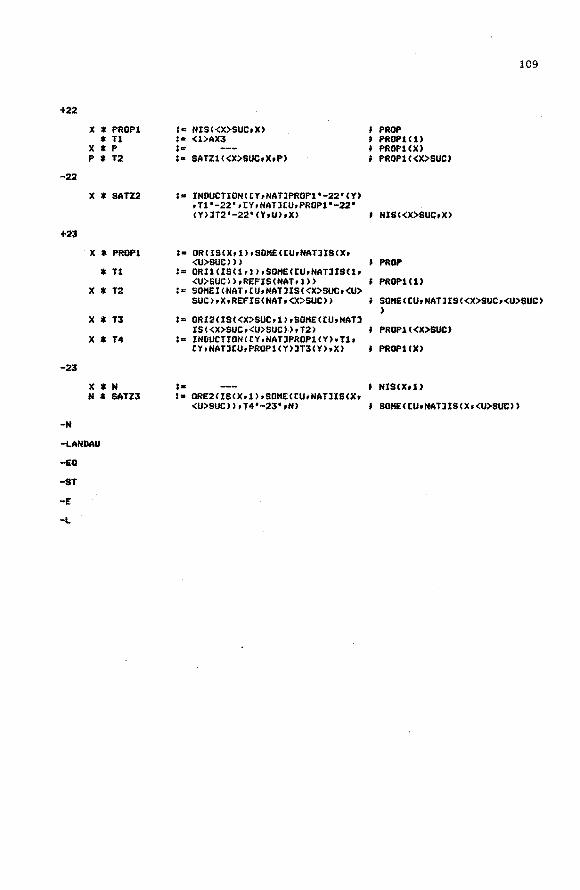
+22
X a PROP1 an
X * p P a T2
-22
X * SATZ2
+23
X * PROP1
*T1
X * T2
X a T3
X * T4
-23
X a N N * SATZ3
-N
-LANDAU
-EG
-ST
-E
-L
l• NIS<<X>SUCoX) l• <1>AX3 , .. I• SATZ1<<X>SUCoXoP)
, .. INDUCTION!tYoNATlPRDP1"-22"(Y) rT1"-22'•tYrNATJtUrPROP1"-22" <Y>JT2"-22"(YrU>rX)
, .. OR<IS<Xrl)oSOKE<tUrNATJISCXr <U>SUC>))
:- ORI1CIS<1•1>•SDHE([U,NATJISC1t <U>SUC>>rREFIS<NATrl>>
I= SOHEI <·NATr tU•NATliS«X>SUCt<U> SUC>rXrREFIS<NATr<X>SUC>>
l= ORI2<IS<<X>SUCr1)rSOKE<tUrNATl IS<<X>SUCr<U>SUC>>•T2>
:= INDUCTI0N([YrNATJPROP1CY)rTlr CY•NATJ[U,PROP1<Y>lT3<Y>•X>
I• I• ORE2<IS<X•1>•SDHECCUrNATliS<Xr
<U>SUC>>rT4•-23"rN>
PROP PROPHU PROP100 PROP1«X>SUC)
f NIS«X>SUCoX)
PROP
PROP1<1)
109
SOHE<CUrNATliS<<X>SUCr<U>SUC) )
PROPl«X>SUC)
PROP1CX)
NIS<Xrl>
SOKE<CUtNATliS<X•<U>SUC))
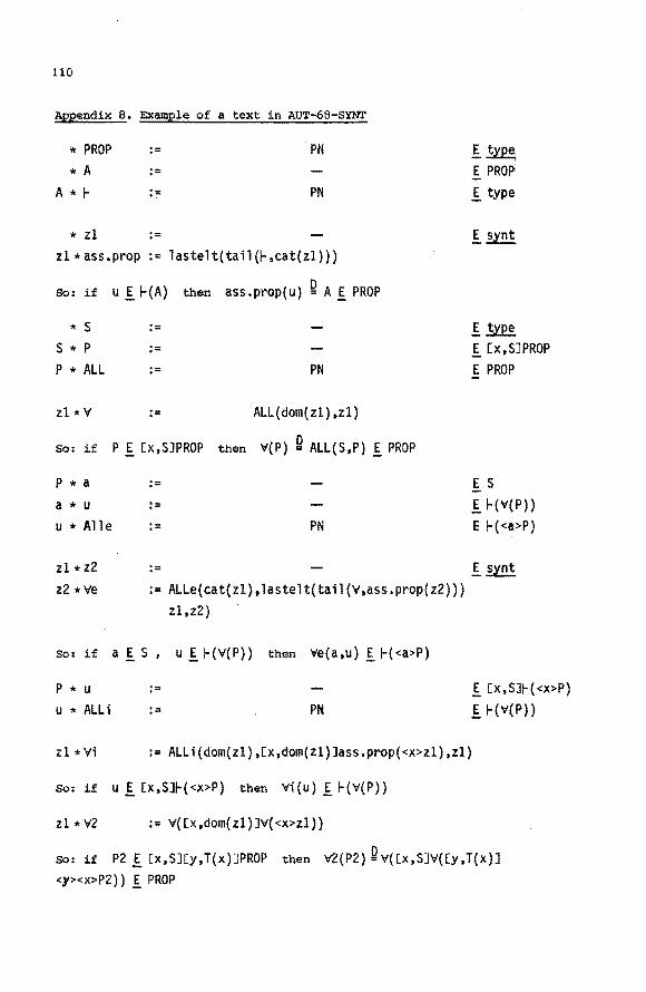
110
Appendix B. Example of a text in AUT-68-SYNT
* PROP .- PN
* A .-A * 1- := PN
* zl .-zl *ass.prop := lastelt(tail(l-,cat(zl))}
So: if u I ~(A} then ass.prop(u) ~ A I PROP
* s .-s * p .-P * ALL .- PN
zl * v .- ALL(dom(zl),zl)
So: if P I [x,SJPROP then V(P) ~ ALL(S,P) I PROP
P * a a * u u * Alle := PN
I~ E PROP
I type
I synt
I~ I [x,SJPROP
E PROP
E S
IHV(P))
E H<a>P)
zl * z2
z2 *Ye
:= I synt
:= ALLe(cat(zl),lastelt(tail(v,ass.prop(z2)))
zl,z2)
so: if a f S , u I 1-(V(P)) then Ve{a,u) I 1-(<a>P)
p * u :=
u * ALLi PN
zl *Vi := ALLi(dom(zl).[x,dom(zl)Jass.prop{<x>zl),zl)
So: if u I [x,SJI-{<x>P) then Vi{u) I 1-(V(P))
zl * v2 := V([x,dom{zl)JV{<x>zl))
I [x,SJH <X>P)
I 1-(V(P))
so: if P2 I [X ,SJ[y, T(x) ]PROP then V2{ P2) Qv( [x ,SJV( [y, T{x) J
<y><X>P2)) I PROP

z2 * z3 z3 * v2e
·.-:= ve(z2,Ve(zl,z3))
111
so: if a f S, b I T(a} , u I ~(V'2(P2)) then V'2e(a,b,u) I~(<b><a>P2)
zl * V'2i := Vi([x,dom(zl)JV'i(<x>zl))
so: if u I [x,SJ[y,T(x)J~(<y><x>P2) then V'2i(u) I ~(V'2(P2})
zl * V'3 := V'([x,dom(zl)JV'2(<x>zl))
so: if P3 I [x,SJ[y,T(x)J[z,U(x,y)JPROP then V'3(P3) Q V'([x,SJV'([y,T{x)J V'([z,U(x,y)]<Z><y><X>P3}}) E PROP
z3 * z4 z4 * V3e
:=
:= V'2e(z2,z3,Ve(zl,z4}}
so: if a IS , b I T(a) , c I U(a,b) , u I ~(V'3(P3)) then
V'3e(a,b,c,u) I r(<C><b><a>P3)
zl * V'3i := V'i([x,dom(zl)JV'2i(<x>zl)}
so: if u I [x,SJ[y,T(x)J[z,U(x,y)JI- (<z><y><x>P3) then V'3i(u) I I-(V'3(P3))
A * 8 .-B * A+B := V([x,I-(A)JB)
z2 * +e := ve(z2,zl} z2 * mod.pon := +e
E PROP E PROP
so: if u I 1-(A+B), vI 1-(A) then +e(u,v) I ~(B), mod.pon(u,v) I 1-(B).
* .L := V([x,PROPJx) E PROP
A*.., := A-+.L E PROP
B * AvB := V'([x,PROPJ((A+x)-+{(B-+x)+x})) E PROP
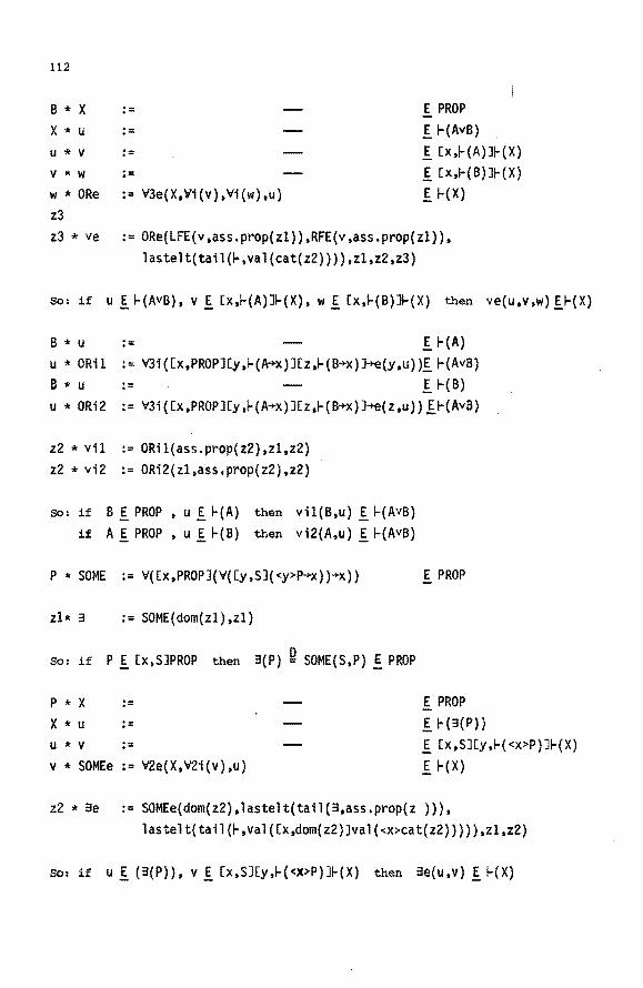
112
B * X
X * u U * V
V * W
w * ORe z3
.-
.-:=
.-:= V3e( X,Vi (v), Vi (w) ,u)
E PROP I 1-(AvB} I [X,I-{A)JI-(X) I [x,I-(B)JI-(X} I 1-(X)
z3 * ve := ORe(LFE(v,ass.prop(zl)),RFE(v,ass.prop(zl)), lastelt(tail(~.val(cat(z2)))),zl,z2,z3)
so: if u I 1-(AvB), vI [x,I-(A)JI-(X), w I [x,I-(B)JI-(X) then ve(u,v,w)II-(X)
B * u := I 1-(A) u * ORil := V3i([x,PROPJ[y,~(A+x)J(z,~(B+x)J~(y,u))I r(AvB) B * u .- I 1-(B) u * 0Ri2 := V3i([x,PROPJ[y,I-(A+x)J[z,I-{B+x)J+e(z,u)) II-(AvB)
z2 * vil := 0Ril(ass.prop(z2),zl,z2) z2 * vi2 := 0Ri2{zl,ass.prop(z2),z2)
so: if B E PROP • u I ~(A) then vil(B,u) I ~(AvB) if A E PROP , u I ~(B) then vi2(A,u) I ~(AvB)
P *SOME := V([x,PROPJ(V([y,SJ(<y>P+x))+x))
Zl* 3 := SOME(dom(zl),zl)
So: if P I [x,SJPROP then 3(P) ~ SOME(S,P) ! PROP
p * X .-X * u .-U * V :=
v * SOMEe := V2e(X,V2i(v),u)
E PROP
E PROP Ir(3(P)) I [x,SJCy.~(<x>P)J~(X)
I 1-(X)
z2 * 3e := SOMEe(dorn(z2),1astelt(tail(3,ass.prop(z ))), lastelt(tail(~.val([x,dorn{z2)Jval(<x>cat(z2))))),zl,z2)
so: if u I (3(P)), vI [x,SJ[y,~(<X>P)J~(X) then 3e(u,v) I ~(X)

a * u u * SOMEi
z3 * 3i
:= V2i([x,PROPJ[z,~{V([y,SJ(<y>P+x)))J V2e(a,u,z))
:= SOMEi(dom(zl),zl,zZ,z3)
113
fi-(3(P))
So: if P f [x,SJPROP, a f S, u f ~(<a>P) then 3i(P,a,u) f~(3(P))
S * a a * b
b * IS
z2 * zl=z2
:=
.-:= V{[p,[X,SJPROPJ(<a>p+<b>p))
:= IS(cat(zl),zl,z2)
So: if a f S, b f S then a=b ~ IS(S,a,b) f PROP
zl * left= zl * right=
:= LFE(=,ass.prop(zl)) := RFE(=,ass.prop(zl))
so: if u f ~(a=b) then left=(u) ~ a, right=(u) ~ b
a * ISi
zl * =i zl * ref=
:= V2i([p,[x,SJPROPJ[y,~(<a>p}Jy)
:= ISi(cat(zl),zl) := =i
so: if a E S then =i(a) f ~(a=a), ref=(a) f ~(a=a)
p * a
a * b
b * u
U * V
V * ISe
:=
.-
:= v2e(P,v,u)
z3 * =e := ISe{dom{zl).zl.left=(z2), right=(z2),z2,z3) z3 * subst.pred := =e
E S
E S
E PROP
E S E S
f 1-(a=b) f 1-(<a>P) f 1-(<b>P)
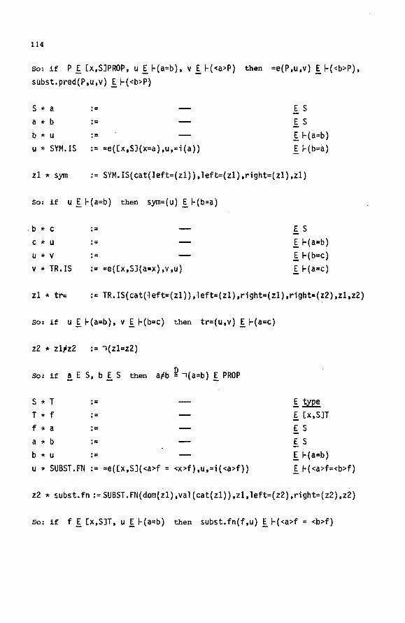
114
so: if P f [x,SJPROP, u f ~(a=b), v f ~(<a>P) then =e{P,u,v) f~{<b>P), subst.pred(P,u,v) f ~{<b>P)
S * a .- E S a * b := E S b * u .- f 1-{a=b) u * SYM. IS := =e{[x,SJ(x=a),u,=i{a)} f 1-{b=a)
zl * sym := SYM.IS{cat{left=(zl)),left=(zl),right=(zl},zl}
So: if u f ~(a=b} then sym=(u) f~(b=a)
. b * c
c * u
U * V
v * TR. IS
:=
.-:= := =e{[x,SJ(a=x),v,u)
E S f 1-{a=b) f 1-{b=c) f 1-{a=c)
zl * tr= := TR.IS(cat{left=(zl)},left=(zl),right=(zl),right=(z2),zl,z2)
so: if u f ~(a=b), v f ~{b=c) then tr=(u,v} f~{a=c)
z2 * zl#z2 := •(zl=z2)
so: if ! E S, b f S then a#b ~ •{a=b) f PROP
s * T .-T * f :=
f * a :=
a * b := b * u .-u * SUBST.FN := =e([x,SJ(<a>f = <X>f),u,=i(<a>f}}
f~ f [x,SJT E S E S
f 1-(a=b) E ~(<a>f=<b>f)
z2 * subst. fn := SUBST. FN{ dom( zl), va 1 ( cat{zl)) ,zl,l eft=( z2) ,right=( z2) ,z2)
so: if f f [x,SJT, u f 1-{a=b} then subst. fn(f ,u) f H <a>f = <'b>f)
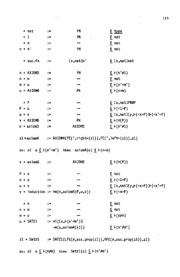
* nat
* 1
* n n * n'
* suc.fn
n * AXIOM3 n * m m * u u * AXIOM4
* p
p * u u * V
V * AXIOMS n * axiom3
zl *'axiom4
.-
.-:= .-
.-
.-
.-
.-
.-
.-:= .-.-.-
PN PN
PN
[x,natJx'
PN
PN
PN AXIOM3
I~ E nat E nat E nat
I [x,natJnat
I 1-(n';l) E nat I 1-(n'=m') I Hn=m)
I [x,natJPROP I 1-( <l>P)
115
I [x,natJ[y,~{<x>P)J~{<x'>P)
If-(V{P)) I Hn';l)
:= AXIOM4{FE{' ,right={zl)),FE(',left={zl)),zl)
so: if u I ~{n'=m') then axiom4{u) I ~{n=m)
v * axiomS .- AXIOMS I f-(V{P))
P * n .- E nat n * u .- I 1-(<l>P) U * V .- I [x,natJ[y,~{<x>P)J~{<x•>P)
v * induction := ve(n,axiomS{P,u,v)) I H <n>P)
* n .- E nat n * m .- E nat m * u .- I f-(n;m) u * SATZl := Vi{[x,~{n'=m')J
+e(u,axiom4{x))) I 1-(n';m'')
zl * Satzl := SATZl{LFE(;,ass.prop{zl)),RFE(;,ass.prop{zl)),zl)
so: if u I ~{n;m) then Satzl{u) I ~{n';m')

116
* P2 := [x,natJ(x';x) n * Satz2 := induction(P2,n,axiom3{l),[x,nat]
[y,r(<x>P2)JSatzl(y))
* P3 := [x,natJ( (x=l)v3([y,natJ(x=y')))
* 11 := v il{3([y,natJ(l=y') ),ref=(l)) n * 12 := 3i([y.natJ{n'=y'),n,ref=(n')) n * 13 := vi2(n'=l, 12) n * 14 := induction(P3,n,13,[x,natJ
Cy,r(<x>P3)Jl3(x)) n * u .-u * SATZ3 := ve{l4,[x,r(n=l)JV2e(x,3([y.natJ
(n=y')),u).Cx,r{3(Cy.natJ(n=y')))Jx)
zl * Satz3 := SATZ3(LFE(;,ass.prop(zl)),zl)
I [x,natJPROP
I f-(n';n)
I [x.natJPROP IH<l>P3) I r(3(Cy,natJ(n'=y'))) I f-(<n'>P3)
I H<n>P3) I f-(nj61)
I r{3(Cy,natJ(n=y')))
So: if u Ir(nj61) then Satz3(u) I r(3([y,natJ(n=y')))

117
Appendix 9. AUT-SYNT
In 4.1.0 we have indicated that for andi the parameters U and V
are essential, while a and b are redundant parameters. If A, B, p and q
can be correctly substituted for a , b , u and V , then A and B can be cal
culated (up to definit±onal equality) from p and q, because A is definitio
nally equal to CAT(p) and B to CAT(q).
Here we introduce an extension of AU'l'OMATH languages, called AUT-SYNT,
in which it is possible to suppress redundant parameters. In this language,
CAT is incorporated as a p~edefined jUnction. For any 2- or 3-expression E,
CAT(E) is the mechanically calculated type of E. It follows that
andi (CAT (p) ,CAT (q} ,p,q) equals andi (A,B,p,q). The extended language moreover
contains variabLes fo~ e:cp~eesione. A basic symbol ~ (which has no de
gree) is added to the language. Variables of type~ (or~ variables)
are to be interpreted as syntactic variables for expressions. There are
no typing restrictions on substitution for such a variable.
Following the AUT-QE text in 4.1.1 we can write in AUT-SYNT:
* zl := zl * z2 .-z2 * ANDI := andi(CAT(zl),CAT(z2),zl,z2)
Now, if A!~, B ! ~, p! A, q ! B then ANDI{p,q) = andi (CAT(p),
CAT(q),p,q) = andi(A,B,p,q)! and(a,b).
Besides CAT we have other predefined functions in AUT-SYNT. They are
defined for certain classes of expressions (just as CAT is defined for 2-
expressions and 3-expressions). We list these functions here with their
semantics. In, the description of the semantics we will frequently use the
clause: "if E reduces to ••• ".We will say e.g. "if E reduces to [x,A]B, •• ".
This is intended to mean: "if [x,A]B is the first abstraction expression in
the reduction sequence, obtatned by reducing E according to the strategy of
the verifying program". Similar meanings are intended in other cases. Every
where in the description E and E1,E2, ••• ,En will denote correct AUT-expres
sions.
predefined function semantics
CAT CAT (E) is the "mechanical type" of the 2- or 3..,.ex
pression E
OOM If E reduces to [x,A]B or CAT(E) reduces to [x,A]B
or CAT(CAT(E)),= [x,A]B then DOM(E) =A,

118
VAL
ARG
FUN
TAIL
LASTELT
PREP ART
Remarks:
If E reduces to [x,A]B and B does not contain x then i
VAL(E) "' B.
If E reduces to <A>B then ARG(E) ==A.
If E reduces to <A>B then FUN(E) = B.
If E reduces to c(A1, ••• ,An) then TAIL(c,E) is the
string of expressions A1 , ••• ,An.
If E1, ••• ,En is a nonempty string of expressions then
LASTELT(E1, ••• ,En) =En.
If E1, ••• ,En is a nonempty string of expressions then
PREPART(E1, ••• ,En) is the string of expressions
E1'''''En-1'
1) Expressions containing ~variables do not have a type. Lines having
such an expression as their middle part do not have a category part.
2) EB-lines which have ~variables in their context can only have synt
as their category part. In other words: on a~ context only~ va
riables may be introduced.
3) The identifiers CAT, DOM, VAL, ARG, FUN, TAIL, PREPART and LASTELT, and
the identifiers defined in terms of these should not be treated as ordi
nary identifiers. In particular the monotonicity of definitional equali
ty (in this case: if A= B then c(A) = c(B) where c is one of these spe
cial identifiers) does not generally apply here. E.g. if f == [x,nat]l
then <1>f ~ <<l>suc>f, while ARG(<l>f) = 1 ~ <l>suc == ARG(<<1>suc>f).
Similar examples can be found for FUN and TAIL.
4) For languages admitting infix expressions there are functions LFE (for
left fixed expression).and RFE (for right fixed expression) with seman
tics:
If E reduces to A c B then·LFE(c,E) ==A and RFE(c,E) • B.
Exaiilples:
1) The first elimination rule for conjunction can be represented in AUT-QE
by adding, on the con text a ! .I?.!.'.2R ; b !. .I?.!.'.2R introduced in 4 • 1 • 0 :
b * u := u * andel. :=
E and(a,b}
E a

119
Then a and b are redundant parameters, for andel and u is an es
sential parameter. In fact, if pis a substitution instance for U , then the
type of p can be expected to reduce to and(A,B) for some A and B, and these
A and B should the be substituted for a and b ,
Therefore, keeping the context zl I synt introduced above, we can add
the AUT-SYNT line
zl * ANDEl .- andel(LASTELT(PREPART(TAIL{and,CAT{zl)))), LASTELT(TAIL(and(CAT(zl))),zl)
Then p! and{A,B) implies ANDEl(p)! A.
we can now indicate a complication which must be kept in mind when using
AUT-SYNT, and which is connected with remark 3 above. Suppose and has
been defined by and := not(imp(a,not(b))) • we may have p, A and B such
that CAT(pl: not(imp(A,not(B))), and then we have andel(A,B,p) !A, but
ANDEl(p) will be incorrect, since CAT(p) does not Peduce to and(A,B).
Even worse complications may occur when using ARG and FUN.
2) In [vD, 3.6] book-equality is introduced. In AUT-SYNT we could add to
this text, on the context zl I synt ; z2 I synt ;
z2 * is := IS(CAT{zl),zl,z2) zl * refis .- REFIS{CAT(zl),zl) zl symis .- SYMIS(CAT{LASTELT{TAIL{is,zl))),
LASTELT(PREPART(TAIL{is,zl))), LASTELT(TAIL(is,zl)),zl)
Then for any type S , if X I S and Y I S 1 equality of X and y could
be expressed by is(x,y) instead of IS(S,x,y) • Moreover, if X E S we have refis(x) I is(x,x) and if pI is(x,y) we have
symis(p) I is(y,x). 3) A text in AUT-68-SYNT, in which the first three theorems of Landau',s
book are proved, appears in appendix 8.

120
References
[dB] N.G. de Bruijn, AUTOMATH, a language for mathematics, Notes (pre-
[dB2]
pared by B. Fowcatt) of a series of lectures in the Seminaire
de Mathematiques Superieures.
Universite de Montreal, 1971.
N.G. de Bruijn, Lambda calculus notation with nameless dummies,
a tool for automatic formula manipulation, with application
to the Church-Rosser theorem.
Indag. Math., 34, 2_, 1972.
[vD] D.T. van Daalen, A description of AUTOMATH and some aspects of
[vD2]
its language theory.
Proceedings of the Symposium on APL. ed. P. Braffort. Paris,
1974.
Appendix 1 in this thesis.
D.T. van Daalen, The language theory of AUTOMATH.
Thesis, Eindhoven University of Technology, to appear 1977.
[J] L.S. Jutting, A translation of Landau's "Grundlagen" in AUTOMATH.
Eindhoven University of Technology, Dept. of Math., 1976.
[L] E. Landau, Grundlagen der Analysis. rd
3 ed., Chelsea Publ. Comp., New York, 1960.
[dV] R. de Vrijer, Big Trees in a A-calculus with A-expressions as
types.
A-calculus and Computer Science, ed. c. Bohm.
Springer, Ber lin-Heidelberg - New Ycrk, 197 5.
[Zl] I. Zandleven, A verifying program for AUTOMATH.
Proceedings of the Symposium on APL. ed. P. Braffort. Paris
1974.
[Z] J. Zucker, Formalization of classical mathematics in AUTOMATH.
To appear in: Actes du colloque international de logique,
Clermont-Ferrand, July 1975, ed. M. Guillaume.
Preprint: Eindhoven University of Technology, Dept. of Math.

Samenvatting
Dit proefschrift bevat een verslag van de vertaling en verificatie van
Landau's "Grundlagen der Analysis", in AUT-QE, een van de AUTOMATH-talen.
Deze talen zijn geconstrueerd met het doel er wiskundige redeneringen in
uit te drukken, met behoud van de herkenbaarheid van de gedachtengang, en
wel zo precies dat mechanische controle (b.v. door een computer) van de
correctheid mogelijk is.
De vertaling werd ondernomen om na te gaan in hoeverre de taal AUT-QE aan
bovenvermelde specificatie voldoet.
In het proefschrift vindt men onder meer een overzicht van de gebruikte
logische axioma's, een verslag van de bij de vertaling ondervonden moeilijk
heden, en een aantal suggesties voor het gebruik van AUTOMATH-talen.
De appendices 4 en 7 bevatten fragmenten uit de vertaling.
De belangrijkste conclusie is dat AUT-QE en andere AUTOMATB-talen in prin
cipe geschikt zijn voor het gestelde doel.
STELLINGEN
I
De moeite die nodig is om (zonder in metamathematische probleemstellingen
te treden) een formele grondslag voor de wiskunde te leggen wordt door veel
wiskundigen overschat.
Litt: dit proefschrift, hfdst. 4. L.s. Jutting, A translation of Landau's "Grundlagen" in AUTOMATH, Eindhoven University of Technology, Dept. of Math., 1976.
Il
Voor formalizering van constructieve en klassieke wiskunde is de oorspron
kelijke AUTOMATa taal AUT-68 toereikend. Een niet essentiele uitbreiding
van deze taal, AUT-68-SYNT, is hiertoe zeer geschikt.
Litt: dit proefschrift, hfdst. 4.
III
De n-reductie verhoogt de uitdrukkingskracht in AUTOMATH-talen niet wezen
lijk.
Litt: dit proefschrift, hfdst. 4.
IV
Ten onrechte wordt algemeen gedacht dat iedere informele bewering van de
vorm "als ••• dan ••• " zonder meer als implicatie te formalizeren is.
Litt: S. Beaumont-R. Pierce,
s. Ackermans-J. v. Lint,
'
The algebraic Foundations of Mathematics, 1963. Readinq-Palo Alto-London, AddisonWesley. Th. 1-7.1, 4-6 problem 9 (f). Algebra en Analyse, 1970. Groningen, WoltersNoordhoff. Definitie 4.3.21, Stelling 5.8.5.
V
De bewering van Martin-L6f dat de door hem beschreven algorithme voor de
vaststelling van definitiegelijkheid geschikt is voor implementatie op een
computer is onjuist.
Litt: P. Martin-LOf, An intuitionistic theory of types, 1975. Proc. Logic Colloquium 1973, H. Rose-J. Shepherdson ed. Amsterdam-Oxford, NorthHolland Publ. eo.

VI
De Leeuws definitie van de beinvloedingsrelatie tussen attributen is vat
baar voor verbetering.
Litt: A.C.J. de Leeuw, Systeemleer en organisatiekunde, 1974. Leiden, Stenfert Kroese.
VII
De resultaten van A.M. Fink over de maximale amplitude van bestuurde slin
geringen kunnen worden verscherpt.
Litt: A.M. Fink, Maximum Amplitude of Controlled Oscillations. Journal of Mathematical Analysis and Applications~· 253-262 (1966).
VIII
De voorrangsregels voor de algebraische bewerkingen op getallen dienen uit
drukkelijk als conventies te worden gepresenteerd.
Litt: Getal en Ruimte, Deel B1, Algebra voor de brugklas, Tjeenk WillinkNoorduijn, Culemborg. Sigma, deel 1, Wolters-Noordhoff, Groningen.
IX
a) Een burgerlijk huwelijk is een juridische overeenkomst.
b) Het is te betreuren dat deze overeenkomst dikwijls wordt aangegaan uit
sociale of anderszins niet zakelijke motieven, en niet met het oog op de
juridische gevolgen van de overeenkomst.
dl Het is gewenst een dergelijke overeenkomst ook mogelijk te maken tussen
meerdere personen en tussen twee personen van hetzelfde geslacht.
Eindhoven, 1 maart 1977. L.s. van Benthem Jutting