Chebyshev II

7/21/2019 Chebyshev II

http://slidepdf.com/reader/full/chebyshev-ii 1/22

C

CHAPTER 5

C HEBYSHEV T YPE II F ILTERS

hebyshev Type II filters are closely related to Chebyshev Type I filters, andare noted for having a flat passband magnitude response, and an equirippleresponse in the stopband. As was noted in Chapter 4, the Chebyshev

Type I response is often simply referred to as the Chebyshev response. Similarly, theChebyshev Type II response is often referred to as the Inverse Chebyshev response,for reasons that will become clear as the response is developed below.

In this chapter the Chebyshev Type II response is defined, and it will beobserved that it satisfies the Analog Filter Design Theorem. Explicit formulas for thedesign and analysis of Chebyshev Type II filters, such as Filter Selectivity , Shaping

Factor, the minimum required order to meet design specifications, etc., will beobtained. From the defining the corresponding H(s) will be determined,and means for determining the filter poles and zeros are found. To complete the studyof lowpass, prototype Chebyshev Type II filters, the phase response, phase delay,group delay, and time-domain response characteristics are investigated.

5.1 EQUIRIPPLE STOPBAND MAGNITUDE

Suppose that is the magnitude-squared frequency response of aChebyshev Type I filter according to (4.1) :

Let be obtained from (5.1) as follows:

Finally, the desired magnitude-squared response is obtained by replacing byin (5.2) :



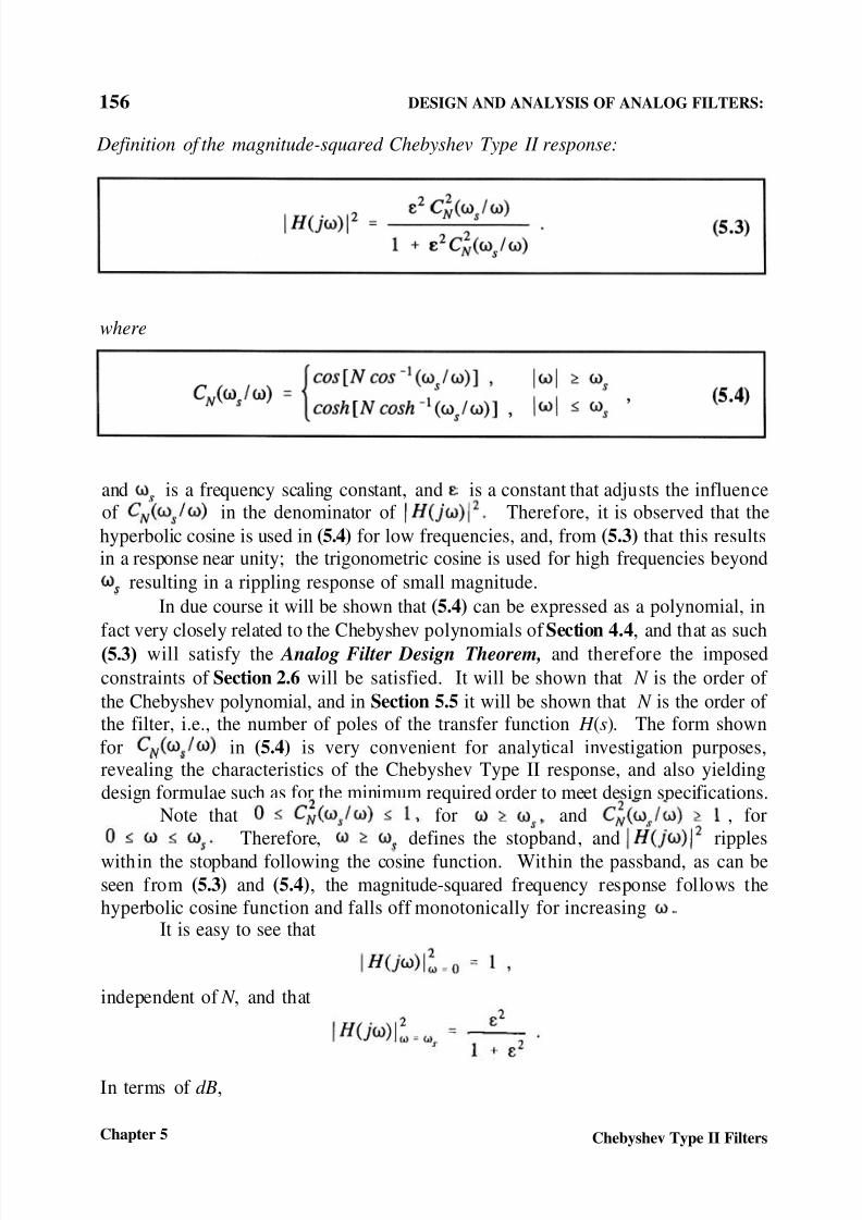
156 DESIGN AND ANALYSIS OF ANALOG FILTERS:

Definition of the magnitude-squared Chebyshev Type II response:

where

and is a frequency scaling constant, and is a constant that adjusts the influenceof in the denominator of Therefore, it is observed that thehyperbolic cosine is used in (5.4) for low frequencies, and, from (5.3) that this resultsin a response near unity; the trigonometric cosine is used for high frequencies beyond

resulting in a rippling response of small magnitude.In due course it will be shown that (5.4) can be expressed as a polynomial, in

fact very closely related to the Chebyshev polynomials of Section 4.4 , and that as such(5.3) will satisfy the Analog Filter Design Theorem, and therefore the imposedconstraints of Section 2.6 will be satisfied. It will be shown that N is the order of the Chebyshev polynomial, and in Section 5.5 it will be shown that N is the order of the filter, i.e., the number of poles of the transfer function H (s). The form shownfor in (5.4) is very convenient for analytical investigation purposes,revealing the characteristics of the Chebyshev Type II response, and also yieldingdesign formulae such as for the minimum required order to meet design specifications.

Note that for and , forTherefore, defines the stopband, and ripples

within the stopband following the cosine function. Within the passband, as can beseen from (5.3) and (5.4) , the magnitude-squared frequency response follows thehyperbolic cosine function and falls off monotonically for increasing

It is easy to see that

independent of N , and that

In terms of dB,

Chapter 5 Chebyshev Type II Filters



A Signal Processing Perspective 157

and

Note that (5.5) is the minimum attenuation for all When (5.5) is comparedwith the general magnitude specifications for the design of a lowpass filter illustratedin Figure 2.15 on page 52, setting equal to the negative of (5.5) results in

Several values of and corresponding values of are shown in Table 5.1 . Notethat is the minimum attenuation in the stopband. At frequencies where thenumerator of (5.3) is zero, the attenuation is infinity.

Note that the magnitude-squared response of (5.3) is zero in the stopbandwhen The frequencies where the response is zero may be found asfollows:

from which

Section 5.1 Equiripple Stopband Magnitude




Therefore, the frequencies where the response is zero are as follows:

where

where if N is odd, and if N is even. Note that if N iseven the highest frequency where the attenuation is equal to is infinity.

The stopband response is denoted as “equiripple” since all of the stopbandpeaks (the points of minimum attenuation) are the same magnitude. It is noted that thefrequency spacing between peaks are not equal: it is the magnitudes of the peaks thatare equal.

The frequency at which the attenuation is equal to a given may be foundfrom (5.3) :

and then solve for making use of the hyperbolic form of (5.4) :

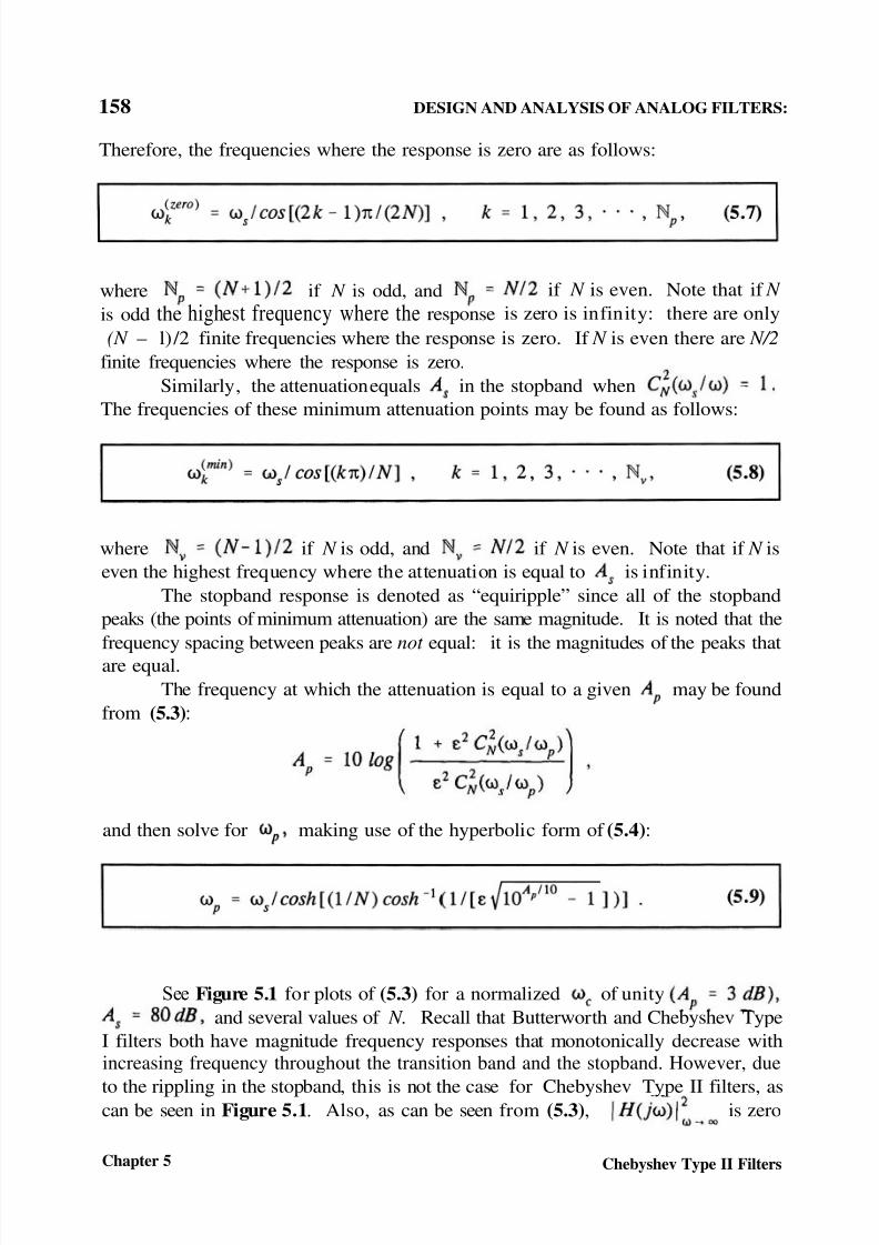
See Figure 5.1 for plots of (5.3) for a normalized of unityand several values of N. Recall that Butterworth and Chebyshev Type

I filters both have magnitude frequency responses that monotonically decrease withincreasing frequency throughout the transition band and the stopband. However, due

to the rippling in the stopband, this is not the case for Chebyshev Type II filters, ascan be seen in Figure 5.1 . Also, as can be seen from (5.3) , is zero


if N is odd, and if N is even. Note that if N is odd the highest frequency where theresponse is zero is infinity: there are only(N – l) /2 finite frequencies where the response is zero. If N is even there are N/2

finite frequencies where the response is zero.Similarly, the attenuationequals in the stopband when

The frequencies of these minimum attenuation points may be found as follows:




if N is odd, and is if N is even. Even though the frequency rangedoes not go to infinity in Figure 5.1 , this phenomenon is observable.

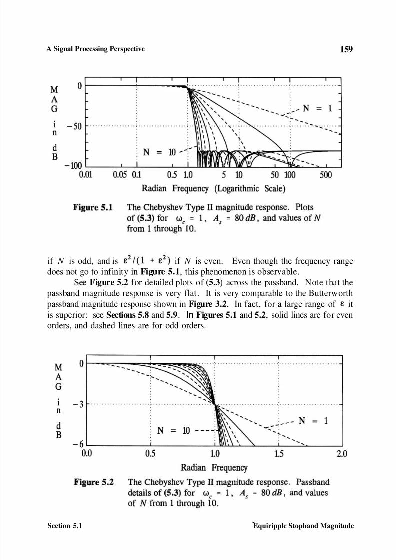
See Figure 5.2 for detailed plots of (5.3) across the passband. Note that the

passband magnitude response is very flat. It is very comparable to the Butterworthpassband magnitude response shown in Figure 3.2 . In fact, for a large range of itis superior: see Sections 5.8 and 5.9 . In Figures 5.1 and 5.2 , solid lines are for evenorders, and dashed lines are for odd orders.

Section 5.1 Equiripple Stopband Magnitude




Example 5.1Suppose N = 5, and then,

from (5.7), the frequencies where the magnitude frequency response is zero are1051.46 rad/s, 1701.3 rad/s, and infinity. From (5.8) the frequencies where theattenuation in the stopband ripples to a minimum of are 1236.07 rad/s and3236 .07 r a d / s . From (5.9),

5.2 FILTER SELECTIVITY AND SHAPING FACTOR

Applying (2.37) , the definition of Filter Selectivity, to the square root of (5.3)results in

If (5.9) is used, with and therefore in (5.10) to eliminate anydirect reference to then (5.10) may be expressed as follows:

It is noted that (5.11) is identical to (4.9) .Let A be an arbitrary attenuation in dB relative to the DC value such that

From (5.3) :

For a given A, solving (5.12) for would be equivalent to solving for the bandwidthat that attenuation A:

Using (5.13) and applying (2.38) , the definition of Shaping Factor, the ChebyshevType II filter Shaping Factor may be readily found:





Example 5.2Suppose a = 3 dB, b = 80 dB, and

From (5.11) , for N = 1, 2, · · · , 10, may be computed to be 0.35, 0.71, 1.06,1.43, 1.84, 2.28, 2.79, 3.35, 3.97 and 4.67 respectively. From (5.14) , for N from1 through 10, may be computed to be 10000.0, 70.71, 13.59, 5.99, 3.69, 2.70,2.18, 1.87, 1.67 and 1.53 respectively.

5.3 DETERMINATION OF ORDER

An important step in the design of an analog filter is determining the minimumrequired order to meet given specifications. Refer to Figure 2.15 on page 52 inspecifying the desired filter magnitude characteristics. As long as the filter magnitudefrequency response fits within the acceptable corridor indicated in Figure 2.15 , itsatisfies the specifications.

Starting with (5.3) :

Temporarily let a real variable, assume the role of N, an integer, as is done inChapters 3 and 4. Therefore, from (5.15) :

from which, making use of (5.6) ,

Letting where is the smallest integer equal to or larger thanthe minimum order required to meet the specifications may be

determined from the following:

Note that (5.16) is identical to (4.14) : for the same specifications, the minimum orderrequired for a Chebyshev Type II filter is the same as that for a Chebyshev Type Ifilter.

Section 5.3 Determination of Order




Example 5.3Suppose the following specifications are given:

and From the right side of (5.16),Therefore, N = 6.

5.4 INVERSE CHEBYSHEV POLYNOMIALS

A recursion for (5.4) may readily be developed, similar to that which was donein Section 4.4 for Chebyshev Type I filters. The resultant recursion is similar to(4.21) :

It is important to note that (5.17) applies equally to the cosine and hyperbolic formsof

If N = 0, and for convenience is normalized to unity,

and therefore

If N = 1 ,

and therefore

For N > 1 the recursion (5.17) may be used. For N = 2 ,

Several Chebyshev polynomials are shown in Table 4.2 . Inverse Chebyshevpolynomials may be obtained from Table 4.2 by replacing with Note thatif is not normalized to unity, the inverse Chebyshev polynomial is as shown inTable 4.2 with replaced by

It can be shown that the square of all inverse Chebyshev polynomials have onlyeven powers of and that multiplied by and added to unity they have no realroots. If they are not added to unity, as appears in the numerator of (5.3) , then theydo have real roots: those roots may be found by (5.7) . Therefore, the Analog Filter

Design Theorem is satisfied. For example, see Example 5.4 .





Example 5.4Suppose N = 3, and Then

and

A root of the denominator requires that

which has no real solution, i.e., no real roots. The numerator has one real repeatedroot, which is 115.47. Therefore, the Analog Filter Design Theorem is satisfied:there is a corresponding H (s) that meets all of the imposed constraints of Section 2.6 .Therefore a circuit can be implemented with the desired third-order Chebyshev TypeII response.

5.5 LOCATION OF THE POLES AND ZEROS

Starting with (5.3) and following the procedure used in Section 2.7 :

The zeros of (5.18) may be found by setting

and solving for the values of The trigonometric cosine form of (5.4) must be usedsince the inverse hyperbolic cosine of zero doesn’t exist:

Solving (5.19) for results in

which, except for the j, is identical with (5.7) . Therefore, the zeros of the transferfunction of a Chebyshev Type II filter are as follows:

Section 5.5 Location of the Poles and Zeros




where is given by (5.7) .The poles of (5.18) may be found by setting

As noted in Chapter 4, since is complex, either form, the cosine or thehyperbolic, is equally valid. Either approach will yield the same equations for findingthe poles.

Since the approach here is identical to the approach used in Section 4.5 , except

that is replaced by it follows that the equivalent to (4.32) wouldbe as follows:

For left-half plane poles:

where

It is interesting to note that the poles of the Chebyshev Type I filter, for anormalized may be expressed as follows:

where


Since then and the hyperbolic form of is perhaps themore appropriate:




and the poles of the Chebyshev Type II filter, for a normalized may beexpressed as follows:

and therefore, the poles are the poles reflected about a unit circlein the plane: the magnitudes are inversely related and the phase angles haveopposite polarity. This inverse relationship between the normalized poles of theChebyshev Type I transfer function and those of the Chebyshev Type II is often notedin the literature, and is implied, as noted above, by contrasting (4.33) and (5.22) . Itis possible to find the poles of a Chebyshev Type II transfer function by first findingthe poles of a Chebyshev Type I transfer function and then converting them into

Chebyshev Type II poles. However, this relationship between normalized polesdoesn’t seem to yield any practical advantage. Direct use of (5.22) is quite adequatefor finding the poles of a Chebyshev Type II transfer function. Also note, bycomparing Tables 4.1 and 5.1 , that practical values for are very different for thetwo transfer functions.

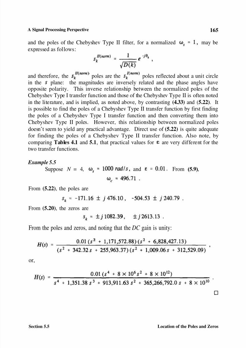
Example 5.5Suppose N = 4 , and From (5.9) ,

From (5.22) , the poles are

From (5.20) , the zeros are

From the poles and zeros, and noting that the DC gain is unity:

or,

Section 5.5 Location of the Poles and Zeros




5.6 PHASE RESPONSE, PHASE DELAY, AND GROUP DELAY

A Chebyshev Type II filter, as seen above, is designed to meet givenmagnitude response specifications. Once the transfer function is determined, it maybe put in the following form:

which is of the form of (2.39) . Given (5.23) , the phase response, from (2.79) , maybe stated as follows:

where and denote the real and imaginary parts of the denominator,respectively, and and denote the real and imaginary parts of thenumerator of (5.23) evaluated with

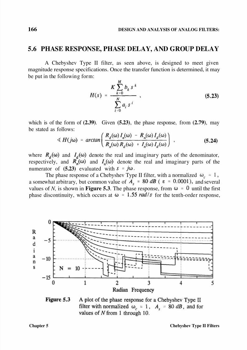
The phase response of a Chebyshev Type II filter, with a normalized

a somewhat arbitrary, but common value of and severalvalues of N, is shown in Figure 5.3 . The phase response, from until the firstphase discontinuity, which occurs at for the tenth-order response,





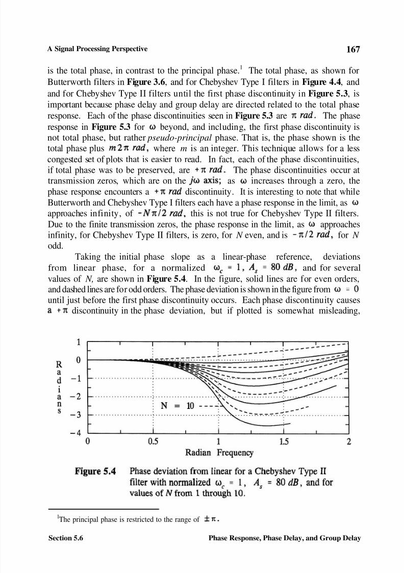
is the total phase, in contrast to the principal phase. 1 The total phase, as shown forButterworth filters in Figure 3.6 , and for Chebyshev Type I filters in Figure 4.4 , andand for Chebyshev Type II filters until the first phase discontinuity in Figure 5.3 , isimportant because phase delay and group delay are directed related to the total phaseresponse. Each of the phase discontinuities seen in Figure 5.3 are The phaseresponse in Figure 5.3 for beyond, and including, the first phase discontinuity isnot total phase, but rather pseudo-principal phase. That is, the phase shown is thetotal phase plus where m is an integer. This technique allows for a lesscongested set of plots that is easier to read. In fact, each of the phase discontinuities,if total phase was to be preserved, are The phase discontinuities occur attransmission zeros, which are on the as increases through a zero, thephase response encounters a discontinuity. It is interesting to note that whileButterworth and Chebyshev Type I filters each have a phase response in the limit, asapproaches infinity, of this is not true for Chebyshev Type II filters.Due to the finite transmission zeros, the phase response in the limit, as approachesinfinity, for Chebyshev Type II filters, is zero, for N even, and is for N odd.

Taking the initial phase slope as a linear-phase reference, deviationsfrom linear phase, for a normalized and for severalvalues of N, are shown in Figure 5.4 . In the figure, solid lines are for even orders,and dashed lines are for odd orders. The phase deviation is shown in the figure from

until just before the first phase discontinuity occurs. Each phase discontinuity causesdiscontinuity in the phase deviation, but if plotted is somewhat misleading,

1The principal phase is restricted to the range of

Section 5.6 Phase Response, Phase Delay, and Group Delay




since the magnitude response is zero at the same frequency and is, in general, in thestopband. Over the frequency range of the figure, phasediscontinuities only effect the plots for orders 8, 9, and 10, as can be seen in thefigure.

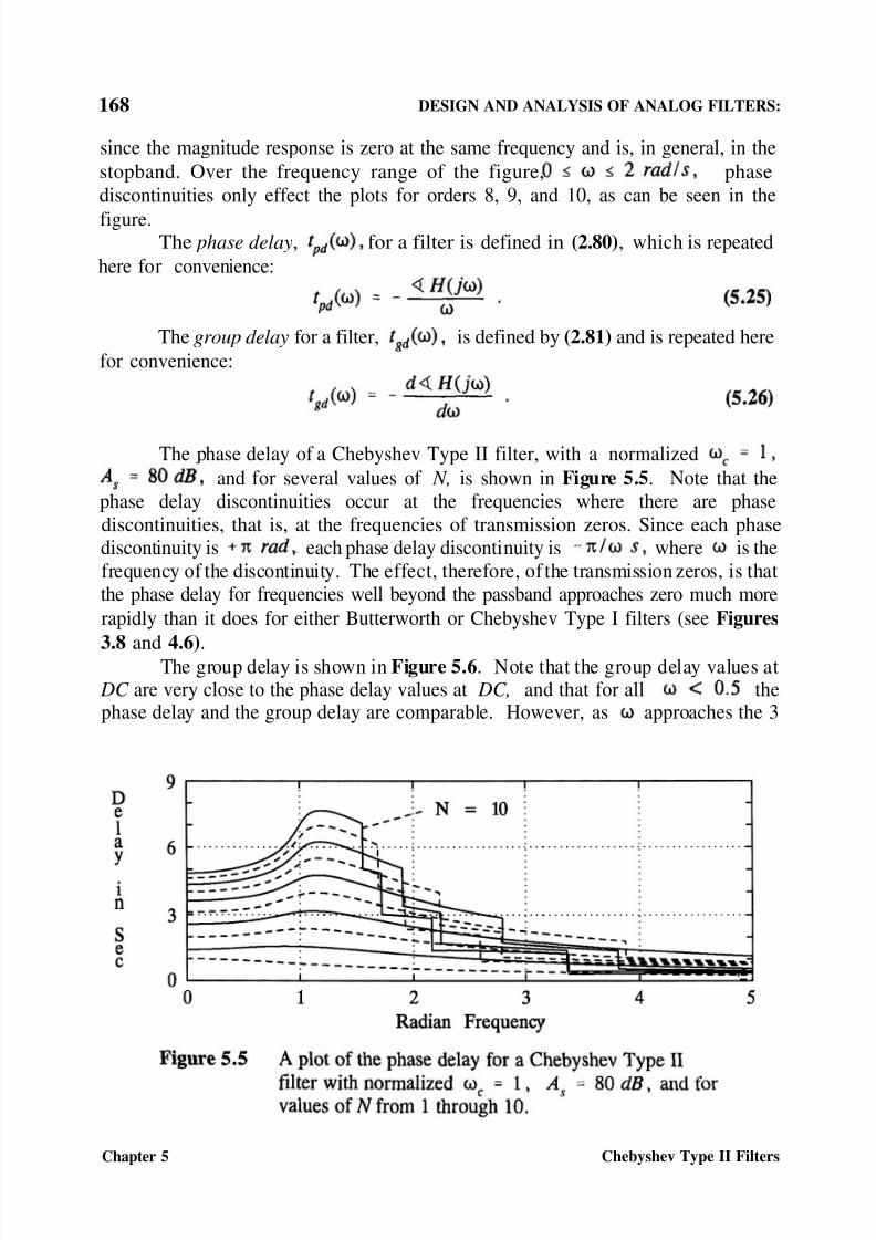
The phase delay , for a filter is defined in (2.80) , which is repeatedhere for convenience:

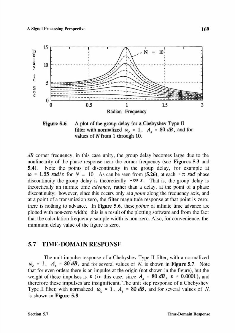
The group delay for a filter, is defined by (2.81) and is repeated herefor convenience:

The phase delay of a Chebyshev Type II filter, with a normalizedand for several values of N, is shown in Figure 5.5 . Note that the

phase delay discontinuities occur at the frequencies where there are phasediscontinuities, that is, at the frequencies of transmission zeros. Since each phasediscontinuity is each phase delay discontinuity is where is thefrequency of the discontinuity. The effect, therefore, of the transmission zeros, is thatthe phase delay for frequencies well beyond the passband approaches zero much morerapidly than it does for either Butterworth or Chebyshev Type I filters (see Figures

3.8 and 4.6) .The group delay is shown in Figure 5.6 . Note that the group delay values at DC are very close to the phase delay values at DC, and that for all thephase delay and the group delay are comparable. However, as approaches the 3





dB corner frequency, in this case unity, the group delay becomes large due to thenonlinearity of the phase response near the corner frequency (see Figures 5.3 and5.4) . Note the points of discontinuity in the group delay, for example at

for N = 10. As can be seen from (5.26) , at each phasediscontinuity the group delay is theoretically That is, the group delay istheoretically an infinite time advance , rather than a delay, at the point of a phasediscontinuity; however, since this occurs only at a point along the frequency axis, andat a point of a transmission zero, the filter magnitude response at that point is zero;there is nothing to advance. In Figure 5.6 , these points of infinite time advance areplotted with non-zero width; this is a result of the plotting software and from the factthat the calculation frequency-sample width is non-zero. Also, for convenience, theminimum delay value of the figure is zero.

5.7 TIME-DOMAIN RESPONSE

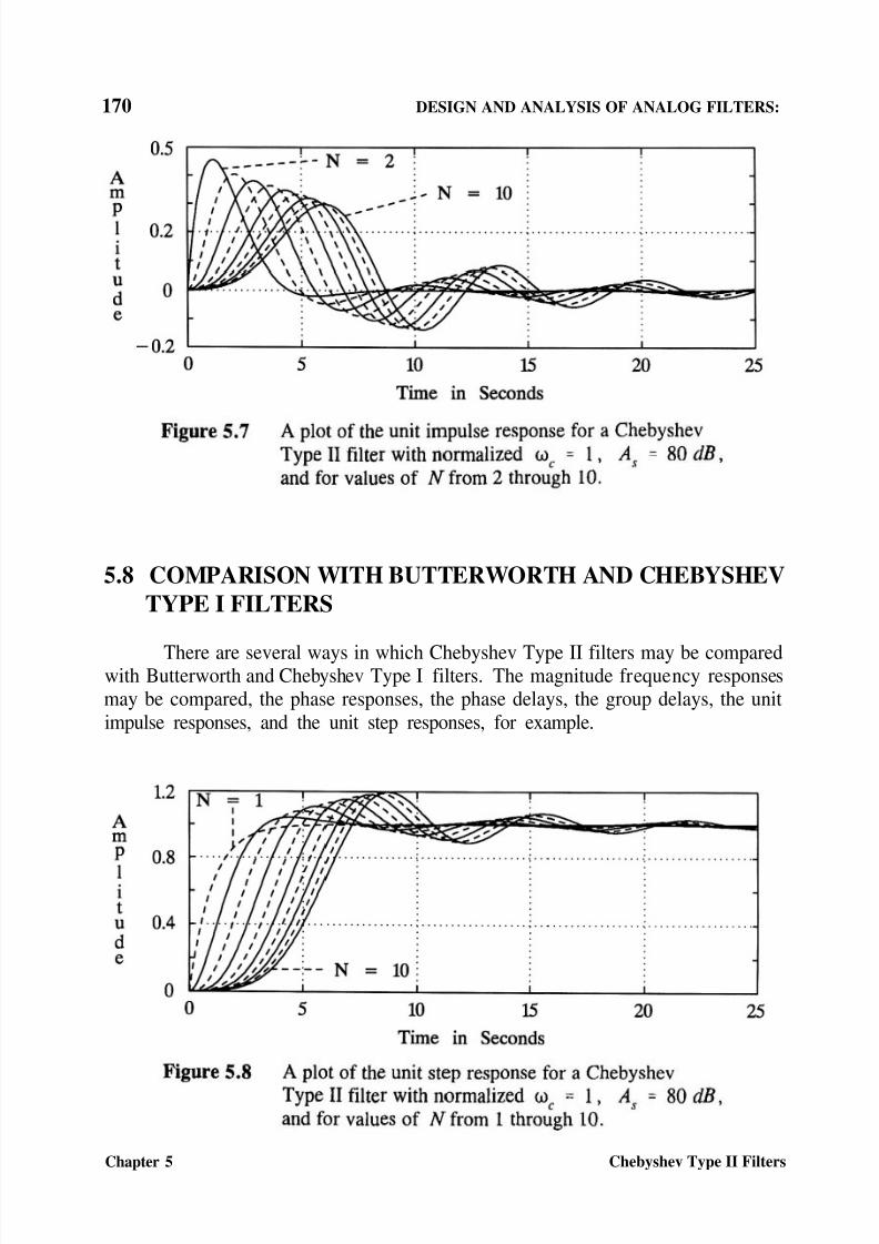
The unit impulse response of a Chebyshev Type II filter, with a normalizedand for several values of N , is shown in Figure 5.7 . Note

that for even orders there is an impulse at the origin (not shown in the figure), but theweight of these impulses is ( in this case, since andtherefore these impulses are insignificant. The unit step response of a Chebyshev

Type II filter, with normalized and for several values of N,is shown in Figure 5.8 .

Section 5.7 Time-Domain Response




5.8 COMPARISON WITH BUTTERWORTH AND CHEBYSHEVTYPE I FILTERS

There are several ways in which Chebyshev Type II filters may be comparedwith Butterworth and Chebyshev Type I filters. The magnitude frequency responsesmay be compared, the phase responses, the phase delays, the group delays, the unitimpulse responses, and the unit step responses, for example.





It is noted that, for a given set of filter specifications, the minimum orderrequired for a Chebyshev Type II response will never be greater than that required fora Butterworth response: it will frequently be less. It is not always less, since theorders are restricted to integers. As noted in Section 5.3 , the minimum order requiredfor a Chebyshev Type II filter is identical with that for a Chebyshev Type I filter.

Although the passband of a Chebyshev Type II response was not designed tobe maximally flat in any sense, yet, as can be seen by comparing Figures 5.2 and 3.2,the passband magnitude response of a Chebyshev Type II filter is comparable with thatof a Butterworth. In fact, over a wide range of filter specifications, the passbandmagnitude response of a Chebyshev Type II filter, with the same order and same3 dB corner frequency, is more flat than that of a Butterworth filter. One way of

demonstrating this is by comparing Filter Selectivity for the two filters. Let (5.11) bedenoted and (3.7) be denoted It can be shown that

for all N, and Equality in (5.27) is achieved only for N = 1 or for verysmall values of For example, for N = 10, and then

It can be shown that, for all practical values of that the Shaping Factor of a Chebyshev Type II filter is always less than that for a Butterworth filter of the sameorder. To illustrate this, compare the results of Example 5.2 to that of Example 3.1 ;in both cases a = 3 dB and b = 80 dB. For example, for N = 8, for theButterworth filter is 3.16, whereas it is only 1.87 for the Chebyshev Type II filter,which indicates that the attenuation in the transition band increases more rapidly as afunction of for the Chebyshev Type II filter than it does for the Butterworth. This,of course, can readily be observed by comparing Figures 3.1 and 5.1.

The above may imply that a Chebyshev Type II filter is superior to aButterworth filter of the same order. However, the phase response of a Butterworthfilter is more nearly linear than is that of a Chebyshev Type II filter of the same order.The differences, however, are not great. The phase deviation from linear for aChebyshev Type II filter, as shown in Figure 5.4 , is greater than it is for aButterworth filter, as shown in Figure 3.7 . This is, of course, reflected in the phasedelay and the group delay, but comparing Figure 5.5 with 3.8 , and 5.6 with 3.9 ,shows that the differences are not great. Comparing plots of the unit impulse responseand the unit step response of the two filters also shows that the differences are notgreat.

The comparison between Chebyshev Type II filters and Chebyshev Type Ifilters is more objective and straight-forward, especially since the minimum required

Section 5.8 Comparison with Butterworth and Chebyshev Type I Filters




order to meet design specifications is identical for both filters. A Chebyshev Type IIfilter, of the same order, has a more constant magnitude response in the passband, amore nearly linear phase response, a more nearly constant phase delay and groupdelay, and less ringing in the impulse and step responses, than does a Chebyshev TypeI filter: compare Figures 5.2 and 4.2, 5.4 and 4.5, 5.5 and 4.6, 5.6 and 4.7, 5.7 and4.8, and 5.8 and 4.9. However, while (5.11) and (4.9) , equations for FilterSelectivity , are the same, the numerical values for differ significantly for the twofilters. For all practical filters, for the Chebyshev Type II filter will besignificantly smaller than that for the comparable Chebyshev Type I filter. Toillustrate this, compare Table 5.1 to Table 4.1 . The result is that, for all practicalfilters, for the Chebyshev Type I filter will be significantly larger than for thecomparable Chebyshev Type II filter: compare Figures 5.2 and 4.2 . However, the

comparison of Shaping Factor values is not consistent. It is possible for a ChebyshevType II filter to have a smaller than a corresponding Chebyshev Type I filter. Toillustrate this, compare 10th-order responses in Figures 5.1 and 4.1 with a = 3 dBand b = 80 dB.

5.9 CHAPTER 5 PROBLEMS

5.1 Given the defining equations for a Chebyshev Type II response, (5.3) and

(5.4), and given that and N = 3 :(a) Determine the value of (b) Determine the value of (c) Determine the frequencies where the response is zero.(d) Determine the frequencies in the stopband where the attenuation is(e) Accurately sketch the magnitude frequency response. Use only a

calculator for the necessary calculations. Use a vertical scale in dB (0to -60 dB ), and a linear radian frequency scale from 0 to 5000 rad/s.

(f) Accurately sketch the magnitude frequency response. Use only a

calculator for the necessary calculations. Use a linear vertical scalefrom 0 to 1, and a linear radian frequency scale from 0 to 2000 rad/s.

5.2 Given the defining equations for a Chebyshev Type II response, (5.3) and(5.4), and given that and N = 6 :(a) Determine the value of (b) Determine the value of (c) Determine the frequencies where the response is zero.(d) Determine the frequencies in the stopband where the attenuation is(e) Accurately sketch the magnitude frequency response. Use only a

calculator for the necessary calculations. Use a vertical scale in dB (0





(f)to -80dB), and a linear radian frequency scale from 0 to 5000 rad/s.Accurately sketch the magnitude frequency response. Use only acalculator for the necessary calculations. Use a linear vertical scalefrom 0 to 1, and a linear radian frequency scale from 0 to 1200 rad/s.

5.3 Starting with (2.37) and the square root of (5.3) , derive (5.11) .

5.4 On page 159 it is mentioned that for a large range of the passband magnituderesponse for a Chebyshev Type II filter is more flat than that of a Butterworthfilter of the same order. On page 171 this concept is expanded upon. Sinceboth responses are relatively flat in the passband, if they both have the samethen the one with the larger Filter Selectivity implies that the magnitudefrequency response remains closer to unity as approaches then does theother one. Verify that, for the same order and the same Filter Selectivityfor a Chebyshev Type II filter is greater than or equal to Filter Selectivity fora Butterworth filter, and that they are equal only for N = 1 or for very smallvalues of That is, verify (5.27) .

5.5 Determine the value of Filter Selectivity for the Chebyshev Type II filterspecified in Problem 5.2. Compare this value with the Filter Selectivity fora Butterworth filter with similar specifications: and

N = 6. Compare this value with the Filter Selectivity for a Chebyshev TypeI filter with similar specifications: and N = 6.

5.6 Determine the value of the Shaping Factor for the Chebyshev Type II filterspecified in Problem 5.2, for a = 3 dB and b = 60 dB. Compare this valuewith the Shaping Factor for a Butterworth filter with similar specifications:

and N = 6. Compare this value with the Shaping Factorfor a Chebyshev Type I filter with similar specifications:

and N = 6.

5.7 Estimate the Shaping Factor for a Chebyshev Type II filter with N = 5 ,and from Figure 5.1. Compare your results with that

obtained from (5.14) .

5.8 Suppose filter specifications are stated as follows:Determine the required filter order to meet the given

specifications:

(a) For a Chebyshev Type II filter with(b) For a Chebyshev Type II filter with(c) For a Chebyshev Type II filter with

Section 5.9 Chapter 5 Problems




For a Chebyshev Type II filter withFor comparison purposes, repeat parts (a) through (d) for a Butterworthfilter.

For comparison purposes, repeat parts (a) through (d) for a ChebyshevType I filter with 0.1 dB of ripple.For comparison purposes, repeat parts (a) through (d) for a ChebyshevType I filter with 0.5 dB of ripple.For comparison purposes, repeat parts (a) through (d) for a ChebyshevType I filter with 1.5 dB of ripple.

(d)(e)

(f)

(g)

(h)

Given that N = 4, and express in poly-nomial form similar to Example 5.4, and demonstrate that it satisfies the

Analog Filter Design Theorem.

Prove that the magnitude-squared frequency response of Problem 5.1 satisfiesthe Analog Filter Design Theorem.

Prove that the magnitude-squared frequency response of Problem 5.2 satisfiesthe Analog Filter Design Theorem.

Determine the 9-th and 10-th order inverse Chebyshev polynomials.

Sketch the square of the 4-th order inverse Chebyshev polynomial forfrom 0 to 1.1 rad/s. Compute the square of (5.4) over this same radianfrequency range for and verify that it is numerically the same as theinverse Chebyshev polynomial.

Determine the poles and zeros of the filter specified in Problem 5.8 (a).

Determine the poles and zeros of the filter specified in Problem 5.8 (d).

Determine the poles and zeros of the filter specified in Problem 5.9 .

Suppose N = 4, and Determine the transferfunction H (s). That is, verify the results of Example 5.5.

Determine the transfer function H (s) for the Chebyshev Type II filterspecified in Problem 5.1. Express the denominator of H (s) in two ways: (1)As a polynomial in s. (2) As the product of a second-order polynomial in s,the roots of which being complex conjugates, and a first-order term. State thenumerical values of the three poles and the finite-value zeros. Sketch the sixpoles and the zeros of H ( -s ) H (s ) on an s plane.


5.9

5.10

5.11

5.12

5.13

5.14

5.15

5.16

5.17

5.18




5.19 Determine the transfer function H (s) for the Chebyshev Type II filterspecified in Problem 5.2 . Express the denominator of H (s) in two ways: (1)As a polynomial in s. (2) As the product of three second-order polynomialsin s, the roots of each second-order polynomial being complex conjugates.Express the numerator of H (s) in two ways: (1) As a polynomial in s. (2) Asthe product of three second-order polynomials in s, the roots of each second-order polynomial being complex conjugates. State the numerical values of thesix poles and six zeros. Sketch the twelve poles and zeros of H (-s) H (s) onan s plane.

5.20 Suppose a Chebyshev Type II filter is be used that has a minimum attenuationof 60 dB at 4000 Hz

(a) If and what is the minimum orderrequired?

(b) If and N = 10, what is the maximum value of ?(c) If and N = 10, what is the minimum value of ?

5.21 Under the conditions of part (c) of Problem 5.20, determine the transferfunction H (s) , and give numerical values for all the poles and zeros.

5.22 Sketch the step response of a 10-th order Chebyshev Type II filter with

and Refer to Figure 5.8 and make use of thescaling property of Fourier transforms. What would the maximum group delaybe for this filter, and at what frequency would it occur? At what time wouldthe peak of the unit impulse response of this filter be, and what would be thevalue of that peak?

5.23

Section 5.9 Chapter 5 Problems

Using the MATLAB functions cheb2ap, impulse and step :(a) Determine the transfer function in polynomial form, and also factored

to indicate the poles and zeros, of a Chebyshev Type II filter withand N = 6.

Determine the impulse response and the step response for the filter of part (a).By multiplying the pole vector and the zero vector found in part (a)by determine the transfer function of a Chebyshev Type IIfilter with and N = 6.Determine and plot the magnitude frequency response of the filter of part (c) by using the MATLAB function freqs. Use a vertical scale indB and a linear horizontal scale from 0 to 5000 Hz. Also determine andplot the phase response over this same frequency range. Use theMATLAB function unwrap rather than plotting the principle phase.By appropriately scaling the impulse response and the step response of

(b)

(c)

(d)

(e)





part (b), determine and plot the impulse response and the step responseof the filter of part (c). That is, the time axis for the step responseneeds to scaled by and the unit impulse response needs

the same time-axis scaling and requires an amplitude scaling of

Determine and plot the phase delay of the filter of part (c). Note thatthis is easily obtained from the phase response of part (d).Determine and plot the group delay of the filter of part (c). Note thatthis also is easily obtained from the phase response of part (d):

where is the phase in radiansat step n, and is the step size in rad/s.

To demonstrate the critical nature of a filter design, this problem experimentssome with the filter of Problem 5.23 (c). Multiply the highest-frequency pole-pair of the filter of Problem 5.23 (c) by 1.1, leaving all other poles and zerosunchanged. Determine and plot the magnitude frequency response of the filterby using the MATLAB function freqs . Use a vertical scale in dB and a linearhorizontal scale from 0 to 5000 Hz. Also determine and plot the phaseresponse over this same frequency range. Use the MATLAB function unwraprather than plotting the principle phase. Compare these results with thatobtained for Problem 5.23 (d).

This problem continues to demonstrate the critical nature of a filter design, andis a continuation of Problem 5.24 . Multiply the lowest-frequency zero-pairof the filter of Problem 5.23 (c) by 1.1, leaving all other poles and zerosunchanged. Determine and plot the magnitude frequency response of the filterby using the MATLAB function freqs. Use a vertical scale in dB and a linearhorizontal scale from 0 to 5000 Hz. Also determine and plot the phaseresponse over this same frequency range. Use the MATLAB function unwraprather than plotting the principle phase. Compare these results with thatobtained for Problem 5.23 (d).

(f)

(g)

5.24

5.25

Chebyshev II

Documents

Transcript of Chebyshev II