Charles I. Jones Macroeconomics - TEST BANK...

Charles I. Jones

Macroeconomics

STUDY GUIDE

Full file at http://testbank360.eu/solution-manual-macroeconomics-1st-edition-jones

Charles I. Jones

Macroeconomics

David GilletteTRUMAN STATE UNIVERSITY

W • W • NORTON & COMPANY • NEW YORK • LONDON

STUDY GUIDE


Copyright © 2008 by W. W. Norton & Company, Inc.

All rights reserved

Printed in the United States of America

Composition and layout: R. Flechner Graphics

First Edition

ISBN 978-0-393-93113-6

W. W. Norton & Company, Inc., 500 Fifth Avenue, New York, NY 10110

wwnorton.com

W. W. Norton & Company Ltd., Castle House, 75/76 Wells Street, London W1T 3QT

1 2 3 4 5 6 7 8 9 0


v

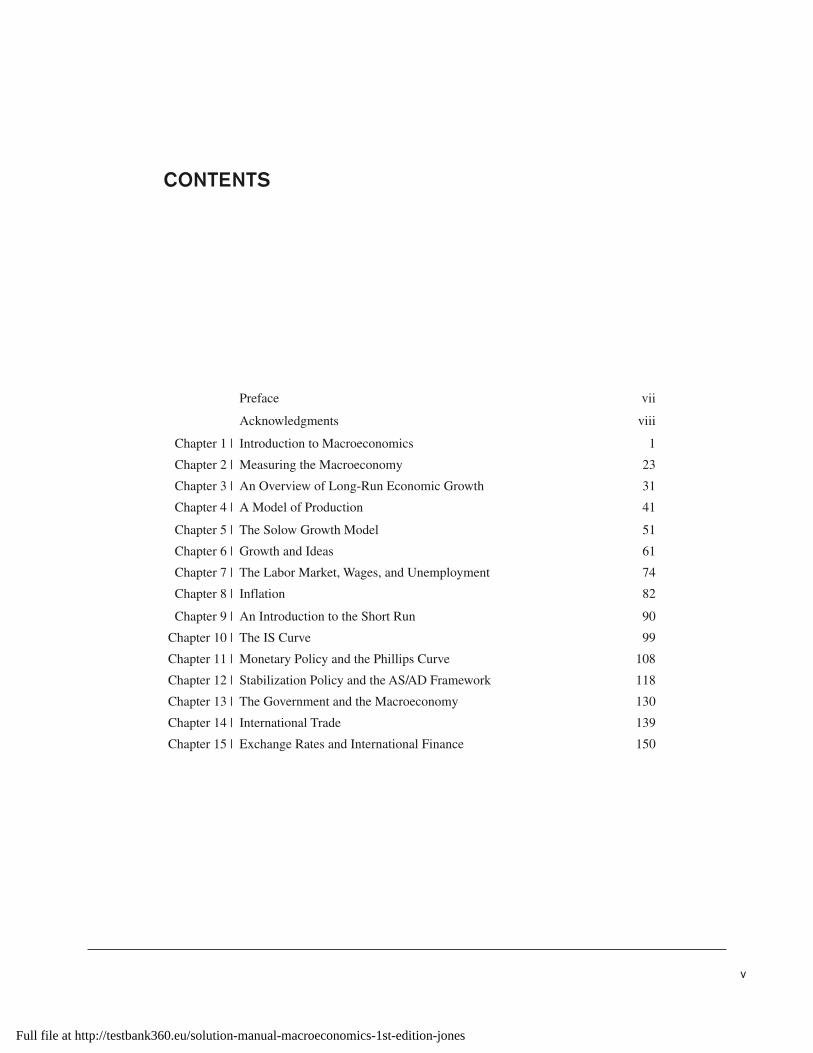
CONTENTS

Preface vii

Acknowledgments viii

Chapter 1 | Introduction to Macroeconomics 1

Chapter 2 | Measuring the Macroeconomy 23

Chapter 3 | An Overview of Long-Run Economic Growth 31

Chapter 4 | A Model of Production 41

Chapter 5 | The Solow Growth Model 51

Chapter 6 | Growth and Ideas 61

Chapter 7 | The Labor Market, Wages, and Unemployment 74

Chapter 8 | Inflation 82

Chapter 9 | An Introduction to the Short Run 90

Chapter 10 | The IS Curve 99

Chapter 11 | Monetary Policy and the Phillips Curve 108

Chapter 12 | Stabilization Policy and the AS/AD Framework 118

Chapter 13 | The Government and the Macroeconomy 130

Chapter 14 | International Trade 139

Chapter 15 | Exchange Rates and International Finance 150


vii

Preface

The purpose of this study guide is to enhance your learningexperience as you work through Charles Jones’s Macro - economics. Each section of each chapter has been carefullydeveloped and reviewed by several students to bestaccomplish this goal. My assumptions in writing eachchapter are that you will have already read the text materialbefore turning to the study guide, that you are now ready tolearn how much you know, and that you want to find outwhere you still need to know more.

Each chapter of the study guide starts with a statementresponding to the learning objectives presented at thebeginning of each chapter in the textbook. This statementprovides a succinct chapter summary in which you shouldrecognize all the major topics. I suggest you test yourselfby thinking about how much more detail concerning eachtopic you could fill in with no further prompting.

The second part of each chapter in the study guide contains a more in-depth explanation for each of the chap-ter’s key concepts. These explanations are meant to ensurethat no major concepts are missed as you read the chapterand, in some cases, provide quick examples or furtherexplanation to supplement the material in the text. Thisinformation on its own is not a substitute for actually read-ing the chapter.

The third and fourth sections provide an opportunity to

test your understanding of chapter material by answeringsome true/false and multiple-choice questions before mov-ing on to the exercises and problems. To make studying asefficient as possible, most concepts receive only a one- question allotment, so challenge yourself. Treat these ques-tions as a self-test and try answering each of them withoutreferring back to the chapter or to the answers at the end ofthe study guide. All the answers for each true/false and multiple-choice questions at the end of the study guideinclude a section reference back to the text, in case you needto do some follow-up studying, and most of them also havean explanation about why an answer is correct. Some evenexplain why a few very tempting answers are incorrect.

The next two sections of each chapter present exercisesand problems intended to help prepare you for the end-of-the-chapter exercises in the textbook. Try to work throughthem on your own at first but do not get discouraged if youget stuck. Early experiences with the modeling aspects ofeconomics can sometimes be quite difficult. Therefore,each exercise and problem also has a solution provided atthe end of each chapter, unless it is one of the worked prob-lems, whose solution follows immediately and serves as aguide for the material that follows.

Best wishes as you pursue your study of macroeconomics.


viii

Acknowledgments

I wish to express my appreciation to all those who havehelped make this study guide become a reality. My thanksgo first, to my best friend, Gabriele, for her continuedfriendship and support over many years and specificallyduring this project, and then to Jack Repcheck and MattArnold of Norton for their encouragement and confidencethroughout this process.

I would especially like to thank Daniel Campbell, JustinJenkel, Samantha Sanchez, and Kathleen Schulte of Tru-man State University, who in addition to their other course-work faithfully read and critiqued each element of thisstudy guide. It benefited immensely from their efforts. Anysurviving errors, of course, remain my responsibility.


1

OVERVIEW

The objectives for Chapter 1 are to learn what macro eco-nomics is, what kinds of questions the text will teach you toaddress, the nature of an economic model, and how econo-mists use it to answer important questions. Macroecono-mists study issues regarding the economy as a whole:economic growth, inflation, unemployment, interest rates,expansions, contractions, fiscal and monetary policies,budget and trade deficits, exchange rates, and the like. Thischapter introduces the questions surrounding these issuessuch as the growth of inflation during the 1970s and the cor-responding roles of both monetary and fiscal policy. Otherquestions concern the behavior and sustainability of our cur-rent trade and budget deficits. This chapter also reviews thebasics of model building.

KEY CONCEPTS

Macroeconomics is the study of collections of people andfirms and how their interactions through markets de ter-mine the overall performance of the economy.

Microeconomics is the study of individual people, firms, ormarkets and how they interact to determine the alloca-tion of particular economic goods.

Economic models allow economists to abstract from aninnumerable set of forces at play in the real world inorder to narrow the focus to a smaller set of forcesthought to be most relevant to the issue at hand. Forexample, an entire market might be represented by twosimple equations, one for demand, Qd = a – bP + cY,and one for supply, Qs = e – fP, and represented on ademand and supply diagram with price, P, on the verti-cal axis and quantity, Q, on the horizontal axis.

Parameters are components of the model, sometimes calledbehavioral or sensitivity parameters, that generallyremain fixed or constant over time unless explicitlychanged by the model builder. For example, if we con-sider the demand equation Qd = a – bP + cY, the lettersa, b, and c are parameters that define the behavior ofdemand, either independent of P and Y, as in the caseof a, or in response to changes in P and Y, as in thecases of b and c, respectively.

Exogenous variables are components of the model that areallowed to change over time but only in specific ways,as determined in advance by the model builder. Forexample, in the preceding demand equation, Y mightbe income that changes by 100, or by 10 percent, andcauses the demand curve to shift by an amount deter-mined in part by the parameter c.

Endogenous variables are the outcomes generated by themodel. For example, a competitive market model

S

D

Q

P

Introduction to MacroeconomicsCHAPTER 1


2 | Chapter 1

combining the demand equation Qd = a – bP + cY withthe supply equation Qs = e – fP would yield a solutionfor price, P, and quantity, Q, in terms of the modelparameters and exogenous variables for that particularmarket.

Long-run economic analysis occurs when there has beensufficient time for all factors of production to adjust tochanges and disturbances in the economy. For exam-ple, in the long run, the size of a factory can beexpanded to meet an increase in demand due to anincrease in population.

Short-run economic analysis occurs when one or more ofthe factors of production in the economic process can-not be changed in response to changes and distur-bances in the economy. For example, in the short run,workers in a factory might have to work overtime tomeet an increase in demand until the factory can beexpanded.

Potential output (GDP) describes the maximum amountthat an economy could produce if all of its factors ofproduction were fully and efficiently employed. It gen-erally is thought of as growing at a steady rate overtime and associated with the long-run behavior of aneconomy.

Economic fluctuations occur in the short run and describethe behavior of actual output relative to potential out-put. Sometimes, a fluctuation will generate a positiveoutput gap, where actual GDP exceeds potential GDPfor a short period of time; at other times, an outputfluctuation will leave actual GDP below potential GDPgenerating a negative GDP gap.

Inflation measures the growth (in percentage terms) of theprice level (an index number) over time and can derivefrom either demand or supply side changes.

TRUE/FALSE QUESTIONS

1. Macroeconomics is to microeconomics as a building isto construction materials.

2. Microeconomics concerns issues of the consumer, firm,and industry, while macroeconomics concerns issues ofthe economy as a whole.

3. For 150 years, the U.S. GDP per capita exceeded thatof most industrialized countries, including the UnitedKingdom, Germany, and Japan.

4. Unemployment generally increased during the last halfof the twentieth century for Europe, Japan, and theUnited States.

5. During the last half of the twentieth century, investmentremained relatively constant at about 20 percent ofGDP.

6. The solutions of an economic model are specific valuesof the endogenous variables.

7. Per capita GDP growth in the United States has aver-aged close to 3 percent for the past 140 years.

8. News announcements about quarterly GDP growthshed light on long-run economic trends.

MULTIPLE-CHOICE QUESTIONS

1. The study of modern macroeconomic theory requiresthe use of techniques froma. game theory.b. all of the social sciences.c. only macroeconomic principles.d. only microeconomic principles.e. both macroeconomic principles and the study of

individual behavior.

2. Which of the following issues is not addressed by thestudy of macroeconomics?a. inflationb. firm behaviorc. budget deficitsd. per capita wealthe. economic growth

3. Which of the following issues is not addressed by thestudy of microeconomics?a. government interventionb. exchange ratesc. opportunity costd. unemploymente. labor markets

4. The study of macroeconomics addresses each of thefollowing issues excepta. recessions.b. unemployment.c. personal income.d. the national debt.e. economic growth.

5. Which of the following issues is not addressed by thestudy of macroeconomics?a. government interventionb. trade barriersc. exchange ratesd. stock pricese. stock market bubbles


Introduction to Macroeconomics | 3

6. Macroeconomists generally follow a four-step processwhen performing their analysis. Which of the followingis not one of those steps?a. Develop a survey.b. Document the facts.c. Develop a model.d. Compare the predictions of the model to the original

facts.e. Use the model to make other predictions that may

eventually be tested.

7. To be considered successful, a model must a. provide solutions for the endogenous economic

variables in question.b. provide correct qualitative descriptions of changes in

the endogenous variables in response to the model’sbehavioral parameters.

c. generate correct quantitative predictions for theendogenous variables in response to changes in theexogenous variables.

d. do all of the above.e. do only a and c.

EXERCISES

This first problem is intended to help familiarize you with theSnapshots resource.

1. Go to http://elsa.berkeley.edu/~chad/snapshots.html;download the Country Snapshots file by clicking on thesnapshots.pdf link and open it. (Some browsers willallow you to work with the file without downloadingit.) Note that pages 3–4 in this file contain detailed

instructions on its use and sources. After openingCountry Snapshots, locate the country “Hungary” inthe list of countries on page 1 and click on it.a. How many years of GDP data are provided?b. What is GDP per capita in the year 2000?c. What does the number you obtain for your answer

on part b mean? (Hint: Click on the link “Click herefor notes” on page 1 then go to the third bullet.)

d. How much does it differ from GDP per worker inthe year 2000?

e. How do GDP per capita and GDP per worker differin principle?

f. What is the GDP growth rate for the year 2000?

Worked Exercise

The following exercise will lead you step by step throughthe process of using a spreadsheet to create a graph. Itassumes very little spreadsheet experience but does requirebasic computer application familiarity, such as selectingcontent, copying, and pasting. The instructions assume theuse of Microsoft Excel on either a PC or a Mac, but theprocedures are similar to other spreadsheet packages aswell.

2. Continuing with the country of Hungary, once you havefound the Snapshots page for Hungary you should see“Hungary(Population=10.0m)(data)” printed at the topof it. Click on the word “data” to download the excelfile for Hungary. (Depending on your computerconfiguration you may need to right-click and selectthe appropriate option. Otherwise, the URL ishttp://elsa.berkeley.edu/~chad/snapshots/HUN.xls)Open it. The file should look as follows (on page 4):


4 | Chapter 1

First, organize the data in a more graphing friendly format for Excel. Thereare several ways to accomplish this, so if you know another one that works wellfor you, please feel free to use it, but for the novice spreadsheet user, this oneshould provide a good place to start. Notice when you first open the original filethat there is only one tab, titled “Sheet1,” at the bottom of the file. Go to theapplication menu bar and click on the “Insert” pull-down menu and select“Worksheet.”



A second tab will appear titled “Sheet2.”

Choose “Sheet1” and, beginning with row 6, column A, select rows 6 through60 and columns A through M inclusive. Using the “Edit” pull-down menu, copythese cells.


Assume for the sake of this exercise that the two observations for educationalattainment in cells J15 and J20 will not be needed. Select cells A4 through M24inclusive. Then, from the “Edit” pull-down menu, select “Delete” and the “Shiftcells up” option when prompted, so that your sheet now looks as follows.Notice, too, that cell A3 now is empty. (Be sure to remove the word “Year” fromcell A3 using the Delete Key rather than using the space bar to make it go away;a cell with a “space” in it is not empty, and Excel knows this.) The point here isthat an empty cell at the top of the leftmost column tells Excel that the values inthis column are horizontal axis labels rather than the first series that you wish tograph. Your spreadsheet should now look like this:

6 | Chapter 1

Select the “Sheet2” tab you just created, put the cursor in cell A1, and select“Paste.” Your spreadsheet should now look like this:



Your spreadsheet now is ready to easily generate a graph. (Have you savedyet?) Excel’s Chart Wizard has four steps. To begin using it, we create a graphof Hungary’s population from 1970 to 2000. Use your cursor to select cellsA3:B34, as shown next.


8 | Chapter 1

Now click on the “Chart Wizard” icon. It is the little bar chart icon below theletter “H” in “Help” in the following diagram, or you can find it in the “Insert”pull-down menu, which also follows, if the icon is not showing on your application.

Step 1 will ask you to choose a chart type. For this exercise, select “Line” andthe first chart sub-type. Step 2 lets you verify the data range and alter it if youwish, or tell Excel that the data are in columns if it has guessed wrong based onthe cells you highlighted. Normally, you will not need to do anything in Step 2.



Step 3 lets you choose various options regarding the graph’s appearance. Thebest way to learn about this option is to simply click on all the tabs and see whatthey allow you to do. For now, since there is only one series and its title is at thetop of the graph, there is no need for a legend; so click on the “Legend” tab anduncheck the “Legend” box. By clicking on the “Titles” tab, you can add axislabels such as “Year” and “Millions of People” to the graph so that its readerunderstands what the graph represents.

Step 4 asks you to make an important decision regarding where you want thegraph placed. The choice depends on what you want to do with it. If you justwant to work with the graph by itself and print it out or copy and paste it toanother application, placing it as a new sheet makes it easier to work with. Afterclicking on “Finish,” the graph will be complete.


10 | Chapter 1

A couple of tips for working with graphs and making them as readable as possibleinclude going to the “View” menu and clicking on “Sized with Window,” so that thegraph expands to fill the entire space available, as shown in the next two diagrams.



At this point, the graph technically is finished, but you can still experimentwith the various presentation options by clicking on the different elements ofthe graph and determining the available options. For example, by double-click-ing, or right-clicking on the gray area, it can be changed to white (saving a lotof ink when printing). Clicking on the axes and other labels can enhance theirappearance by making them bold or increasing their size. Any number of thegraph’s attributes can be changed; the best way to learn, short of reading aninstruction manual, is just to click and explore. The important part about thisprocess is to produce an easily read and interpreted graph. For example, fromthe graph that follows, we easily can see that the Hungarian population grewduring the 1970s and steadily decreased during the 1980s and 1990s.


12 | Chapter 1

As a concluding exercise to the production of this first graph, look back at thelast three graphs and decide for yourself, which one is the most appealing tostudy and learn from.

Finally, suppose you need to graph more than one data series and those dataseries do not lie in adjacent columns. Copying and pasting them so that they dois one approach to making such a graph. Another, more efficient method, isexactly the same except for the initial step of data selection for the graph. First,select the data in cells A3:A34 on Sheet2, then hold down the control key on aPC or the command key on a Mac (the one with the apple on it) and, while hold-ing it down, select the data in cells D3:D34 and then repeat the process to selectthe data in cells F3:F34 so that your spreadsheet appears as follows. You canrepeat this process to include as many data series as desired.



PROBLEMS

Worked Problem

This problem addresses the issue of modeling that Chapter 1asks you to review from your previous economics course-work. Economists build models using mathematics—partic-ularly algebra, its corresponding graphs, and calculus—tohelp understand the economy. Consider for example, amodel of the market for laptop computers. We are fairly cer-tain that the supply of laptop computers depends on theprice for which they sell and the price of the materialsrequired for their production. We also are fairly certain thedemand for laptop computers depends on the price of laptopcomputers, the price of desktop computers, and consumers’income. We use symbols and notation to express conceptssuch as these more compactly. Recall from your mathclasses that Y = F(W, X, Z) represents a multivariate function where Y is affected by the three variables W, X, andZ. In economics, we adopt this format and express demand

Now click on the Chart Wizard and repeat the process used to produce yourfirst graph. Experiment by clicking on the various components of the graph (cen-ter gray area, axes, legend, titles, series, etc.), changing them until you havematched the graph that follows next. Note that, if you just click on the legendonce, you can drag it around and place it wherever you want it.

and supply functions as Qd = D(P, PDT, Y, . . .);Qs = S(P, PM, . . .). These demand and supply functions indi-cate that several variables have an impact on quantities bothdemanded and supplied. Qs, Qd, P, PDT, PM, and Y are allvariables, denoting, respectively, the quantity of laptopssupplied and demanded, the price of laptops, the price ofdesktop computers, the price of materials, and aggregateconsumer income. In a specific product market like this one,P and Q (both Qd and Qs) are the endogenous variablesbecause the model determines their outcomes. We use otherletters, generally lower case or Greek, to denote constants,exogenous variables (determined outside the model), andbehavioral, or sensitivity, parameters that describe one vari-able’s response to another. Very often in economics, we donot know the exact nature of the relationships among vari-ables so we prefer this type of general functional notation.We also illustrate these relationships on a diagram, where anupward sloping supply curve shows that the quantity of laptops supplied increases and the quantity of laptopsdemanded decreases as the price of laptops rises. PDT, PM,


14 | Chapter 1

and Y are placed inside the parentheses to show that Qd andQs also depend on other variables as well as the price of lap-tops. When working with graphs, like demand and supplydiagrams, the number of endogenous variables is limited totwo: price and quantity (P and Q) and they are always foundon the graph’s axes. Any exogenous variables shift either thedemand or the supply curve and behavioral parametersaffect the slopes.

1. Suppose the following model represents supply anddemand in the market for laptop computers:

Qd = a – bP + cY ? dPDT Qs = eP + fPM

In the problem and calculations that follow do not letthe question mark distract you; we will get to it later.For now, just let a = 300, b = 10, c = 40, d = 30,e = 300, and f = 100.

a. Which variables are exogenous and which areendogenous? How can you tell?

The variables P, Qs, Qd. are the endogenousvariables in this model because they are the outputsdetermined by the model through the solutionprocess. The variables PM, PDT, Y are the exogenousvariables in this model and must be known inadvance (given) in order to find a solution. It alsohelps to note that we find the endogenous variableson the axes (price and quantity) in our demand andsupply diagram.

b. What do the parameters a–f represent, and what istheir function in the model?

The lower case letters, a–f, are behavioral, orsensitivity, parameters. They indicate how anendogenous variable responds to changes of eitherexogenous or endogenous variables found in themodel. For example, the parameter c in the demandequation determines how much quantity demandedchanges in response to an increase in consumerincome.

c. Which sign (+ or –) should replace the questionmark in the demand equation? Why? What would aplus or minus sign signify in the laptop computermarket? The question mark should be replaced witha + sign because laptops and desktops are substituteproducts for performing computing operations.When the price of desktops goes up so does thequantity of laptops demanded, because they becomerelatively less expensive to purchase. Similarly, theuse of a – sign would indicate the presence of acomplementary product, such as a piece of computer software. When the price ofcomplementary products such as software and otherperipherals rises, the quantity of laptops demandeddecrease.

d. What are the equilibrium price and quantity in amarket-clearing model for computers given theassumption of flexible prices? Let income (Y) equal10,000, the price of materials (PM) equal 1,000 andthe price of desktops (PDT) equal 1,200.

First, to generate a solution to this demand andsupply model, it is necessary to impose theequilibrium condition of demand equals supply.Begin, therefore, by setting demand equal to supply,that is, set Qd equal to Qs, then solve first for P thenfor Q as follows:

e. Graph the markets for laptops and desktops labelingeach diagram as completely as possible given theavailable information. With flexible prices yourdiagram should look like this:

300 10 40 30 300 100

300 10 400 000

− + + = +− +

P Y P P P

PDT M

, ++ = +==

36 000 300 100 000

310 336 300

1 084 84

, ,

,

, .

P

P

P

QQ = =+425 452 300 1 084 84

100 000

, ( , . )

,

S

D

QLaptops

P

1,084.84

425,452

S

D

QDesktops

P

1,200



Note that you do not have enough information tocomplete the diagram for the market for desktopcomputers.

f. Suppose income increases to 11,000 and prices inthe laptop market are sticky in the short run. Whatwill be the price and quantity outcomes in the laptopmarket under these conditions? Show them on thelaptop diagram from part e. With sticky prices yourdiagram should look like this:

g. What would the laptop market outcomes be if priceswere flexible and income rose to 11,000? Showthese outcomes on a laptop diagram as you did inpart e. What amount of either inflation or deflationoccurs in the laptop market? With flexible pricesyour calculations will be as they were in part d:

With flexible prices your diagram should now looklike this:

Since the price increases to 1,213.87 from 1,084.84,laptop prices experience inflation of 11.89 percent

h. Suppose instead that desktop prices increase to1,300 (income remains at 10,000 since we now arechanging just the price of the substitute) and thatprices in the laptop market are flexible. What willthe price and quantity outcomes in the laptop marketbe under these conditions? Show these results on aseparate diagram. When desktop prices increase thecalculations are as follows:

Following an increase in the price of a substitute thediagram would be as follows:

S

D0

D1

QLaptops

P

1,084.84

1,094.52

425,452 428,356

300 10 40 30 300 100

300 10 400 000

− + + = +− +

P Y P P P

PDT M

, ++ = +==

36 000 300 100 000

310 336 300

1 094 52

, ,

,

, .

P

P

P

QQ = =+

421 903 300 1 094 52

100 000

, ( , . )

,

1 213 87 1 084 84

1 084 840 1189 11 89

, . , .

, .. . %

− =⎛or

⎝⎝⎜⎞⎠⎟

.

S

D0

D1

QLaptops

P

1,084.84

1,213.87

425,452 464,161

S

D0

D1

QLaptops

P

1,084.84

425,452 465,452

P = 1 084 84, . (remember they are sticky

and do not change)

Qd P Y P

Qd PDT= − + +

= −300 10 40 30

300 10 ++ += −=

440 000 36 000

476 300 10 1 084 84

46

, ,

, ( , . )Qd

Q 55 452,

300 10 40 30 300 100

300 10 440 000

− + + = +− +

P Y P P P

PDT M

, ++ = +==

36 000 300 100 000

310 376 300

1 213 87

, ,

,

, .

P

P

P

QQ = =+

464 161 300 1 213 87

100 000

, ( , . )

,


16 | Chapter 1

2. This problem gives you an opportunity to practice theskills learned in Problem 1 and in the text. Consider thefollowing two diagrams.

S

D

Priceof Oil

NominalInterest

Rates

Barrels ofCrude Oil

LoanableFunds

S0

D

a. What are the endogenous variables in the model ofthe market for crude oil?

b. What are the endogenous variables in the model ofthe market for loanable funds?

c. What are two of the exogenous variables in themarket for oil found in part a? Name at least one forsupply and one for demand.

d. What are two of the exogenous variables in themarket for loanable funds found in part b? Name atleast one for supply and one for demand.

e. Describe and show on the diagram from part a whathappens when the exogenous demand variable youchose for part c increases.

f. Describe, and show on the diagram from part b,what happens when the exogenous supply variableyou chose for part d increases.

CHAPTER 1 SOLUTIONS

True/False Questions

1. True. Modern macroeconomics is built uponmicroeconomic foundations, or individual behavior.

2. True. Macroeconomic issues affect some aspect of thewhole economy, generally related to the standard ofliving.

3. False. See Figure 1.1. The United Kingdom exceededthe United States in the late 1800s.

4. False. See Figure 1.2. Since the mid-1980s, the UnitedStates has experienced a downward trend in itsunemployment rate.

5. False. See Figure 1.4. It is true that investment as apercentage of GDP has been relatively constant but notat 20 percent of GDP, rather at about 16 percent.

6. True. See Figure 1.5. Parameters and exogenousvariables come together to provide an outcome orsolution for an economic model.

7. False. See Figure 1.6. GDP growth has averaged about2 percent since 1870.

8. False. See Section 1.3. News releases about quarterlyGDP behavior generally describe short-termfluctuations, not long-run economic growth.

Multiple-Choice Questions

1. e, both macroeconomic principles and the study ofindividual behavior

2. b, firm behavior

3. d, unemployment

4. c, personal income

5. d, stock prices

6. a, develop a survey

7. d, all of the above

Exercises

1. Snapshots exercise.a. 30. See the top left-hand diagram for Hungary. The

data go from 1970 to 2000 on the horizontal axis.b. 31.4. The number given in parentheses above each

graph identifies the value of the last data point forthat series in the diagram.



c. The number 31.4 means that Hungarian GDP percapita is 31.4 percent of GDP per capita in theUnited States.

d. GDP per worker (39.5) is greater than GDP percapita (31.4). This means that GDP per worker inHungary relative to the United States is 8.1percentage points greater than is GDP per capita(39.5 – 31.4 = 8.1).

e. GDP per worker should always be greater than GDP per capita since not everyone in a country isemployed.

f. The GDP growth rate of approximately 5 percent isgreater than the average growth rate of 2.21 percent(the dotted green line), but it is not possible to tellprecisely from the plot provided.

2. Worked exercise. Answers are given in the exercise.

Problems

1. Worked modeling problem. Answers are given in theproblem.

2. Practice with models of markets.a. The endogenous variables in this model (found on

the axes) are the number of barrels of crude oil andthe price of crude oil.

b. The endogenous variables in this model (found onthe axes) are the amount of loanable funds and theinterest rate.

c. Demand variables exogenous to this model wouldinclude a number of things, such as the demand forheating oil, gasoline, plastics, and natural gas, sincethey are either produced from crude oil or, as in thecase of natural gas, are a substitute for crude oil.Additionally, fuel efficiency in the transportationindustry and insulation in buildings can alsoinfluence (shift) the demand for crude oil. Supplyvariables exogenous to this model would includethings such as the depth of the oil well and thequality of the crude oil. Additionally, the taxes (andsubsidies) levied by government will have an impacton the supply curve, causing it to shift either to theleft or to the right, as will the price of labor and thelevel of government regulation over the oil industry.In short, a change in any variable in the crude oilmarket other than the price of oil or the number ofbarrels produced or demanded will cause either thedemand or the supply curve to shift.

d. Demand variables exogenous to this model include anumber of things, such as the demand for investmentcapital by firms, the size of federal budget deficitsand therefore the government’s need to borrow, orjust the demand for automobile loans by consumers.Additionally, consumer confidence and attitudestoward debt also can influence (shift) the demand for

loanable funds. Supply variables exogenous to thismodel include things such as banks’ attitude towardrisk, individuals’ willingness to postponeconsumption and save instead of spend, and theFederal Reserve interest rate policy. Additionally,the level of expected inflation has an impact on thesupply of loanable funds causing it to shift either tothe left when its higher or to the right when itslower. In short, a change in any variable in theloanable funds market other than the nominalinterest rate or the quantity of loans demanded orsupplied cause either the demand of the supply curveto shift.

e. When an increase in the demand for gasoline orheating oil occurs, it causes the demand for crude oilto increase from D0 to D1, as shown Figure 1.

Figure 1

f. When the Fed increases its bond purchases in theopen market, it causes the supply of loanable fundsto increase from S0 to S1, as shown in Figure 2.

Figure 2

D

S0

S1

NominalInterest

Rates

LoanableFunds

S

D0

D1

Priceof Oil

Barrels ofCrude Oil


18 | Chapter 1

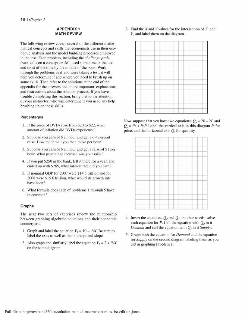
APPENDIX 1 MATH REVIEW

The following review covers several of the different mathe-matical concepts and skills that economists use in their eco-nomic analysis and the model building processes employedin the text. Each problem, including the challenge prob-lems, calls on a concept or skill used some time in the textand most of the time by the middle of the book. Workthrough the problems as if you were taking a test; it willhelp you determine if and where you need to brush up onsome skills. Then refer to the solutions at the end of theappendix for the answers and, more important, explanationsand instructions about the solution process. If you havetrouble completing this section, bring that to the attentionof your instructor, who will determine if you need any helpbrushing up on these skills.

Percentages

1. If the price of DVDs rose from $20 to $22, whatamount of inflation did DVDs experience?

2. Suppose you earn $16 an hour and get a 6¼ percentraise. How much will you then make per hour?

3. Suppose you earn $16 an hour and get a raise of $1 perhour. What percentage increase was your raise?

4. If you put $250 in the bank, left it there for a year, andended up with $265, what interest rate did you earn?

5. If nominal GDP for 2007 were $14.5 trillion and for2008 were $15.6 trillion, what would its growth ratehave been?

6. What formula does each of problems 1 through 5 havein common?

Graphs

The next two sets of exercises review the relationship between graphing algebraic equations and their economiccounterparts.

1. Graph and label the equation Y1 = 10 – 1/2X. Be sure tolabel the axes as well as the intercept and slope.

2. Also graph and similarly label the equation Y2 = 2 + 3/4Xon the same diagram.

3. Find the X and Y values for the intersection of Y1 andY2 and label them on the diagram.

Now suppose that you have two equations: Qd = 20 – 2P andQs = 8/3 + 4/3P. Label the vertical axis in this diagram P, forprice, and the horizontal axis Q, for quantity.

4. Invert the equations Qd and Qs; in other words, solveeach equation for P. Call the equation with Qd in itDemand and call the equation with Qs in it Supply.

5. Graph both the equation for Demand and the equationfor Supply on the second diagram labeling them as youdid in graphing Problem 1.



6. Find the values for P and Q at the intersection ofDemand and Supply and label them on the diagram.Suppose that you have the following equation: C = 50 + 3/4Y, where C stands for an individual’sconsumption and Y stands for income.

7. Draw and label this function, including the axes,intercept, and slope, on the diagram to the right.

8. Provide an economic interpretation for the intercept.

9. Provide an economic interpretation for the slope.

10. Draw and label a second equation representing theincome earned on the graph using the equation Y = Y.

11. At what level of income will this person’s consumptionneeds be met?

Math Skills

Simplify each of the following, except as noted.

1.

2.

3. 6x3 + 4x2y + 2x2z

4.

5. Factor y(3y2 + 7y +2)

6.

7.

8.

9.

10.

11.

12.

13. 2y = 3x + 6, given x = 1/2y

14. Solve for y: y = a + by + c + d – ey

15.

16.

Challenge Problems

The following problems resemble those you will encounterin subsequent chapters in the text, but they might seem unfa-miliar to you now. Do not worry though; the solution processis explained in the answer section and again in the chapterswhere you will need to apply these skills. So, for now, workthe problems as far as you can; then go to the answers andsee how you did or how to complete the problem.

1. For yt = xtazb

t, what is the growth rate of yt?

2. For , what is the growth rate of yt?

3. For

4. Solve for x when

5. If a < 1, what is the solution to y = 100(1 + a + a2 + . . . + an), for n = 14 and n = ∞?

6. Suppose you will receive an inheritance of $10,000 infive years and the interest rate is 6 percent. What is thelowest price for which you would sell that inheritanceright now?

7. Suppose you were to receive $1,000 today and eachyear for the next nine years but that the interest rate isonly 5 percent. What is the lowest price for which youwould sell that inheritance right now?

Math Review Solutions

PERCENTAGES

One of the most frequently used mathematical principles ineconomics is the percentage change of a variable. From inflation to GDP growth, the formula is the same, just thecontext varies. The percentage change (%DX), or growth rate

(gX), of a variable X is when comparing two%ΔXX X

X=

−1 0

0

5 21

xa a( )4 2

2xa( )

51

2x−

3 1 2 2 3 1y y x x x/ −( )[ ] +{ }

−( ) −( )−2 33 13xy xy

3 42x y x( )( )

yx=

3

27.

y x zx

z

y

z= ⎛

⎝⎜⎞⎠⎟ =100 100

12

12

12

show that .

yx

ztta

tb= 100

For findy x yx= ∂

∂6 3 , .

For findy x z yx= ∂

∂61

2 , .

a

a b+

ab

cd

a b c

ab ac

+( )+

4 31

x xa a( )( )−


20 | Chapter 1

values of a variable or when comparing the

current period’s value to that from the last period.

1. DVD inflation: .

2. New wage: $16 + $16(0.0625) = $16(1 + 0.0625) =$16(1.0625) = $17.

3. Raise: . You should

take a moment and confirm that

and $16 + $16(0.0625) = $17, in fact, are equivalent toeach other.

4. Interest earnings: .

5. GDP growth:

6. They each use some version of the percentage change,or growth rate, formula as shown previously. The basic

form of that formula is .

GRAPHS

Supply and demand diagrams are one of economists’ pri-mary tools, of course. Problems 1–3 and 4–6 transform themathematician’s use of a graph into an economist’s use of asupply and demand diagram.

PROBLEMS 1–3

Note: Y2 has a positive slope and represents a direct rela-tionship between X and Y. Similarly, Y1 has a negative slopeand represents an indirect, or inverse, relationship betweenX and Y. To solve for the intersection of Y1 and Y2, set thetwo equations equal to each other and solve for X. Then,substitute X back into either equation to obtain the value forY, where Y1 = Y2.

PROBLEMS 4–6

To invert the Qs and Qd equations, solve each of them for P:

The Supply equation for graphing purposes becomes P = –2 + 3/4Qs, the Demand equation becomes P = 10 – 1/2Qd, andthe solution process is the same as in Problems 1–3.

The solution for Problems 4–6, or the market clearing priceand quantity, is a price of $5.20 and a quantity of 9.6 units.

As a postscript to problems 1–6, note that in both sets ofinitial equations in Problems 1–3 and 4–6, X and P are theindependent variables and Y and Q the dependent variables.Economists, however, have a longstanding tradition of plac-ing Price on the vertical axis and Quantity on the horizontalaxis. This dates back to the time of Alfred Marshall, who

Slope = –1/2 Supply

Demand

Slope = 3/4

Intercept =10

Intercept = –2

50 10

0

5

10

P

Q

Intersection: (9.6, 5.2)

gX X

XXt t

t

= − −

−

1

1

Slope = –1/2

Slope = 3/4

Intercept =10

Intercept = –2

50 10

0

5

10

Y

X

Intersection: (9.6, 5.2)

Y1

Y2

$ $

$. %

265 250

250

15

2500 06 6

− = = =

$ $

$.

17 16

160 0625

− =

$ $

$. . %

17 16

16

1

160 0625 6 25

− = = =

π = − = = =22 20

20

2

20

1

100 1 10. %or

GDP GDP

GDP2008 2007

2007

15 6 14 5

14 5

−= − =$ . $ .

$ .

gX X

X

X X

XXt t t

t

=− − −

−

0

0

1

1

or

1 1.

114 50 075862 7 6

.. . %.= ≈

Q P

P Q

P Q

d

d

d

= −= −= −

20 2

2 20

10 12

Q P

P Q

P Q Q

s

s

s s

= += − += − ( ) + = − +

83

43

43

83

34

83

34

342

10 2

12

1248

59 6

10

12

34

54

45

11

2

− = − +=

= ( ) = =

= −

X X

X

X

Y

.

99 6 5 2

2 9 6 5 2

9 6 5 2

23

4

. .

. .

, . , .

( ) == − + ( ) =

( ) = ( )Y

X Y



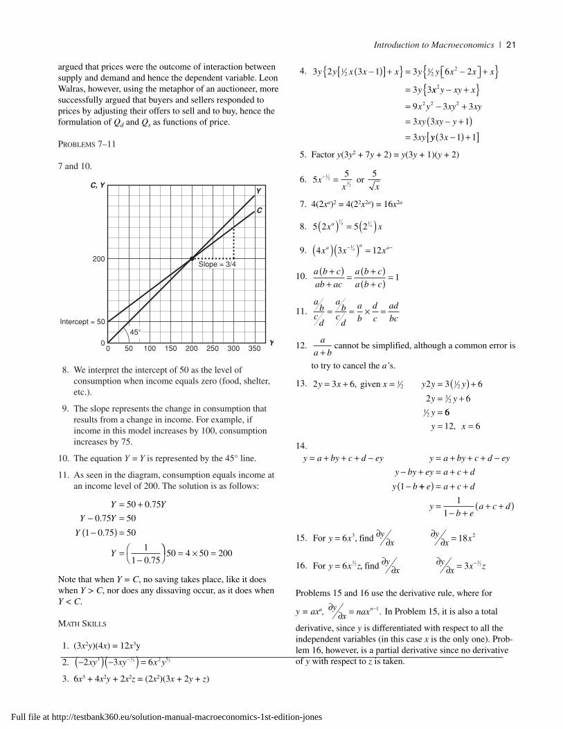
argued that prices were the outcome of interaction betweensupply and demand and hence the dependent variable. LeonWalras, however, using the metaphor of an auctioneer, moresuccessfully argued that buyers and sellers responded toprices by adjusting their offers to sell and to buy, hence theformulation of Qd and Qs as functions of price.

PROBLEMS 7–11

7 and 10.

8. We interpret the intercept of 50 as the level ofconsumption when income equals zero (food, shelter,etc.).

9. The slope represents the change in consumption thatresults from a change in income. For example, ifincome in this model increases by 100, consumptionincreases by 75.

10. The equation Y = Y is represented by the 45° line.

11. As seen in the diagram, consumption equals income atan income level of 200. The solution is as follows:

Note that when Y = C, no saving takes place, like it doeswhen Y > C, nor does any dissaving occur, as it does when Y < C.

MATH SKILLS

1. (3x2y)(4x) = 12x3y

2.

3. 6x3 + 4x2y + 2x2z = (2x2)(3x + 2y + z)

4.

5. Factor y(3y2 + 7y + 2) = y(3y + 1)(y + 2)

6.

7. 4(2xa)2 = 4(22x2a) = 16x2a

8.

9.

10.

11.

12. cannot be simplified, although a common error is

to try to cancel the a’s.

13.

14.

15.

16.

Problems 15 and 16 use the derivative rule, where for

y = axn, In Problem 15, it is also a total

derivative, since y is differentiated with respect to all theindependent variables (in this case x is the only one). Prob-lem 16, however, is a partial derivative since no derivativeof y with respect to z is taken.

∂∂ = −yx naxn 1.

For findy x z yx

yx x z= ∂

∂∂

∂ = −6 31

21

2,

For findy x yx

yx x= ∂

∂∂

∂ =6 183 2,

y a by c d ey y a by c d ey

y by ey a c d

y b

= + + + − = + + + −− + = + +

−1 ++( ) = + +

=− +

+ +( )

e a c d

yb e

a c d1

1

2 3 6 2 3 6

2 6

12

12

32

12

y x x y y y

y y

y

= + = = ( ) += +=

, given

66

12 6y x= =,

a

a b+

Slope = 3/4

Intercept = 50

50

45°

100 150 200 250 300 35000

200

YC, Y

C

Y

−( ) −( ) =−2 3 63 213

83xy xy x y

Y Y

Y Y

Y

Y

= +− =−( ) =

=−

⎛⎝

50 0 75

0 75 50

1 0 75 50

1

1 0 75

.

.

.

.⎞⎞⎠ = × =50 4 50 200

55 51

21

2x

x x− = or

3 2 3 1 3 6 2

3 3

12

12

2y y x x x y y x x x

y

−( )[ ] +{ } = −⎡⎣ ⎤⎦ +{ }= xx y xy x

x y xy xy

xy xy y

xy

2

2 2 29 3 3

3 3 1

3

− +{ }= − +

= − +( )= yy x3 1 1−( ) +[ ]

ab

cd

ab

cd

a

b

d

c

ad

bc= = × =

a b c

ab ac

a b c

a b c

+( )+

= +( )+( ) = 1

4 3 121 1x x xa a aa( )( ) =− −

5 2 5 21 1

x xa a a( ) = ( )


22 | Chapter 1

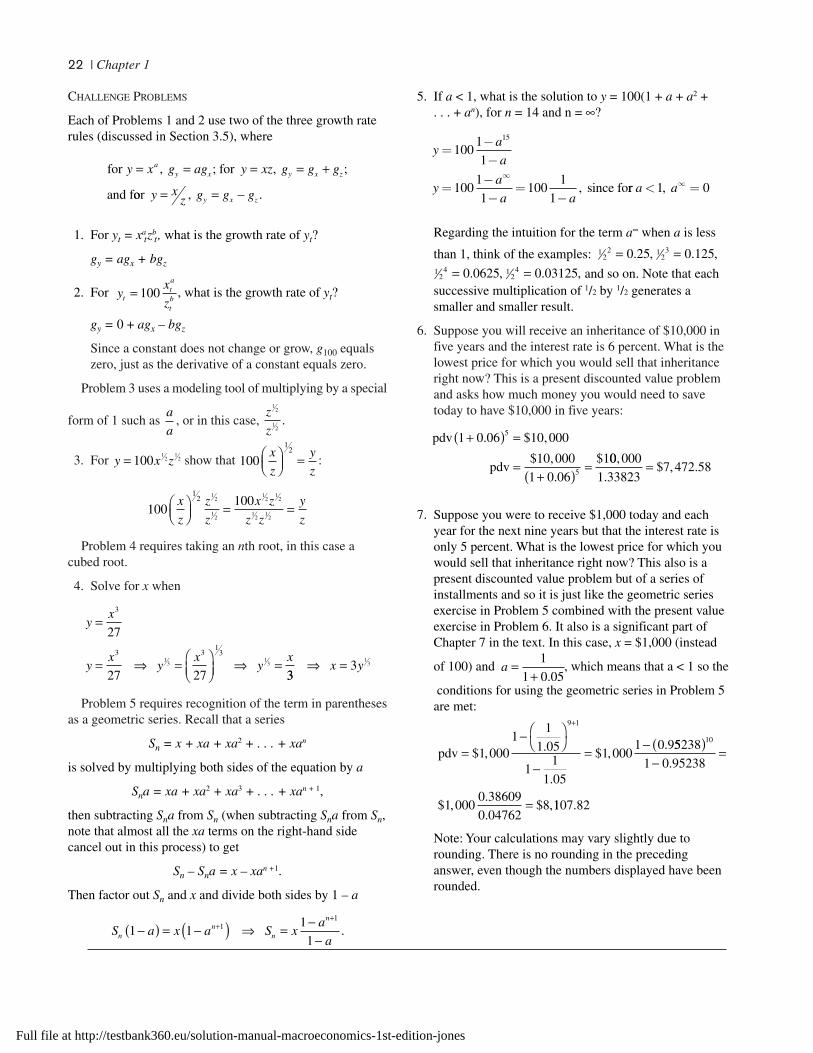
CHALLENGE PROBLEMS

Each of Problems 1 and 2 use two of the three growth raterules (discussed in Section 3.5), where

1. For yt = xatz

bt, what is the growth rate of yt?

gy = agx + bgz

2. For , what is the growth rate of yt?

gy = 0 + agx – bgz

Since a constant does not change or grow, g100 equalszero, just as the derivative of a constant equals zero.

Problem 3 uses a modeling tool of multiplying by a special

form of 1 such as , or in this case,

3. For show that :

Problem 4 requires taking an nth root, in this case acubed root.

4. Solve for x when

Problem 5 requires recognition of the term in parenthesesas a geometric series. Recall that a series

Sn = x + xa + xa2 + . . . + xan

is solved by multiplying both sides of the equation by a

Sna = xa + xa2 + xa3 + . . . + xan + 1,

then subtracting Sna from Sn (when subtracting Sna from Sn,note that almost all the xa terms on the right-hand side cancel out in this process) to get

Sn – Sna = x – xan +1.

Then factor out Sn and x and divide both sides by 1 – a

5. If a < 1, what is the solution to y = 100(1 + a + a2 + . . . + an), for n = 14 and n = ∞?

Regarding the intuition for the term a∞ when a is less

than 1, think of the examples:

and so on. Note that eachsuccessive multiplication of 1/2 by 1/2 generates asmaller and smaller result.

6. Suppose you will receive an inheritance of $10,000 infive years and the interest rate is 6 percent. What is thelowest price for which you would sell that inheritanceright now? This is a present discounted value problemand asks how much money you would need to savetoday to have $10,000 in five years:

7. Suppose you were to receive $1,000 today and eachyear for the next nine years but that the interest rate isonly 5 percent. What is the lowest price for which youwould sell that inheritance right now? This also is apresent discounted value problem but of a series ofinstallments and so it is just like the geometric seriesexercise in Problem 5 combined with the present valueexercise in Problem 6. It also is a significant part ofChapter 7 in the text. In this case, x = $1,000 (instead

of 100) and , which means that a < 1 so the

conditions for using the geometric series in Problem 5are met:

Note: Your calculations may vary slightly due torounding. There is no rounding in the precedinganswer, even though the numbers displayed have beenrounded.

pdv =− ⎛

⎝⎞⎠

−= −

+

$ , .

.

$ ,.

1 0001

1

1 05

11

1 05

1 0001 0 9

9 1

55238

1 0 95238

1 0000 38609

0 047628

10( )−

=

=

.

$ ,.

.$ ,1107 82.

a =+

1

1 0 05.

pdv

pdv

1 0 06 10 000

10 000

1 0 06

1

5

5

+( ) =

=+( ) =

. $ ,

$ ,

.

$ 00 000

1 338237 472 58

,

.$ , .=

yx

yx

yx

yx

=

= ⇒ =⎛⎝⎜

⎞⎠⎟

⇒ =

3

3 31

3

27

27 271

31

3

333

13⇒ =x y

100100

12 1

2

12

12

12

12

12

x

z

z

z

x z

z z

y

z⎛⎝⎜

⎞⎠⎟ = =

1001

2x

z

y

z⎛⎝⎜

⎞⎠⎟ =y x z= 100

12

12

z

z

12

12

.a

a

yx

ztta

tb= 100

for ; for ;

and f

y x g ag y xz g g gay x y x z= = = = +, ,

oor y xz g g gy x z= = −, .

12

4 12

40 0625 0 03125= =. , . ,

12

2 12

30 25 0 125= =. , . ,

ya

a

ya

a a

=−−

=−−

=−

∞

1001

1

1001

1100

1

1

15

, since forr a a< =∞1 0,

S a x a S xa

ann

n

n

1 11

11

1

−( ) = −( ) ⇒ = −−

++

.


Charles I. Jones Macroeconomics - TEST BANK...

Documents

Transcript of Charles I. Jones Macroeconomics - TEST BANK...