Charged Particle Concepts for Fog Dispersion - NASA Particle Concepts for Fog Dispersion ... Charged...
122
NASA Contractor Report 3440 Charged Particle Concepts for Fog Dispersion Walter Frost, Frank G. Collins, and David Koepf CONTRACT NASS-33541 JUNE 1981 https://ntrs.nasa.gov/search.jsp?R=19810018106 2018-06-24T11:16:26+00:00Z
Transcript of Charged Particle Concepts for Fog Dispersion - NASA Particle Concepts for Fog Dispersion ... Charged...

NASA Contractor Report 3440
Charged Particle Concepts for Fog Dispersion
Walter Frost, Frank G. Collins, and David Koepf
CONTRACT NASS-33541 JUNE 1981
https://ntrs.nasa.gov/search.jsp?R=19810018106 2018-06-24T11:16:26+00:00Z

II
NASA Contractor Report 3440
Charged Particle Concepts for Fog Dispersion
Walter Frost, Frank G. Collins, and David Koepf F WG Associates, IHC. Tullaboma, Te)ljressee
Prepared for Marshall Space Flight Center under Contract NAS&33541
National Aeronautics and Space Administration
Scientific and Technical Information Branch
TECH LIBRARY KAFB, NM
1981

ACKNOWLEDGMENTS
The work reported herein was supported by the National Aeronautics
and Space Administration, Marshall Space Flight Center, Space Sciences
Laboratory, Atmospheric Sciences Division, under Contract NAS8-33541.
The authors are indebted to Mr. A. Richard Tobiason of the Office
of Aeronautics and Space Technology (OAST), NASA Headquarters, Washington,
D.C., for his support of this research. Special thanks are given to
Mr. Dennis W. Camp of Marshall Space Flight Center who was the scientific
monitor of the program and who provided considerable technical advice
and input to the final documentation. Also, the authors are appreciative
of the technical discussions with various personnel of the FAA, Naval
Research Laboratories and Energy Innovations, Inc.
ii

TABLE OF CONTENTS
SECTION PAGE
1.0 INTRODUCTION . . . . . . . . . . . . . . . . . . . . . . . . . 1
2.0 CHARGED PARTICLE FOG DISPERSAL CONCEPT AND BACKGROUND RESEARCH . . . . . . . . . . . . . . . . . . . . . . . . . . . 3
2.1 Summary of the Full-Scale Field Experiment in the Panama Canal Zone........................ 6
2.1.1 Description of Experimental Apparatus . . . . . . . 8
2.1.2 Parameters Measured and Instrumentation . . . . . . 12
2.2 Test Results . . . . . . . . . . . . . . . . . . . . . . . 16
2.3 Reported Conclusions from the Field Tests ........ 22
3.0 NOZZLE CHARACTERISTICS .................... 25
3.1 Particle Charging in a Corona Discharge ......... 25
3.1.1 Field Charging .................. 28
3.1.2 Diffusion Charging . . . . . . . . . . . . . . . . 35
3.1.3 Charged Particle Mobility ............. 38
3.2 Previous Nozzles ..................... 54
3.3 Models of Field External to Nozzle Exit ......... 60
4.0 FOG/JET FLUID DYNAMICS .................... 70
4.1 Momentum Equation .................... 72
4.2 Conservation Equations for Water Substances . . . . . . . 74
4.2.1 Governing Equations . . . . . . . . . . . . . . . . 74
4.2.2 Mathematical Expressions for Sources and Sinks of Water Substances . . . . . . . . . . . . . . . . . 76
4.2.3 Water Substance Parameters . . . . . . . . . . . . 78
4.3 Thermodynamic Equations . . . . . . . . . . . . . . . . . 81
iii

SECTION PAGE
4.4 Equations Governing Electrical Properties ........ 81
4.4.1 Governing Equations ............... 81
4.4.2 Ion Attachment to Droplets ............ 85
4.4.3 Release of Free Ions Due to Evaporation ..... 91
4.4.4 Polarization Charging Mechanism ......... 91
4.4.5 Charge Transfer During Coalescence ........ 94
4.5 Utility of Equations .................. 94
5.0 FIELD EXPERIMENT ....................... 96
5.1 General Requirements .................. 96
5.2 Required Measurements .................. 97
5.2.1 Three-Dimensional Wind Field ........... 100
5.2.2 Temperature and Humidity Fields ......... 100
5.2.3 Visibility .................... 100
5.2.4 Cloud Physics .................. 101
5.2.5 Electric Field .................. 101
5.3 Instrumentation ..................... 101
6.0 CONCLUSIONS ......................... 106
iv

LIST OF ILLUSTRATIONS
FIGURE
2.1
2.2
2.3
2.4
2.5
2.6
2.7
2.8
3.1
3.2
3.3
3.4
3.5
3.6
3.7
3.8
3.9
3.10
Principle of Charged Particle Fog Dispersal Technique [2-41 .
Panama Canal Zone Field Experiment Arrangement [2-71 . . . . .
Typical Electric Field Mapping (relative ground-current density distribution) as Reported in Reference [2-4] . . . . .
Charged Particle Spray Gun in Operation [2-71 . . . . . . . .
Schematic of Spray Gun Nozzle [2-41 . . . . . . . . . . . . .
Illustrates Measurement of Load Voltage and of Short- Circuited Current [2-41 . . . . . . . . . . . . . . . . . . .
Schematic of Charged Particle Spray Gun Unit Used in Panama Experiment [2-41 . . . . . . . . . . . . . . . . . . . . . . .
Test Results of the Panama Field Experiment as Reported in Reference [2-71 . . . . . . . . . . . . . . . . . . . . . . .
Operating Principle of Charged Particle Fog Dispersal Technique [3-71 . . . . . . . . . . . . . . . . . . . . . . .
Physics of Corona Discharge [3-91 . . . . . . . . . . . . . . 27
Potential and Flux Lines Around an Uncharged Spherical Particle [3-9, 3-143 . . . . . . . . . . . . . . . . . . . . .
Dipole Induced in Spherical Particle Due to Presence of Nearby Charged Particle [3-91 . . . . . . . . . . . . . . . . . . . .
Potential and Field Lines Around a Partially Charged Spherical Particle [3-143 . . . . . . . . . . . . . . . . . . . . . . .
Field Lines Around a Fully Charged Spherical Particle [3-91 .
Charge Buildup for a Field Charged Particle [3-91 . . . . . .
Charge to Mass Ratio for Spherical Particles in Air [3-lo] . .
Diffusion Charging According to White's Equation [3-81 . . . .
Mobility of Field Charged Particles as a Function of Time Spent in a Corona Discharge . . . . . . . . . . . . . . . . .
5
7
9
10
11
13
14
17
26
29
29
30
30
33
34
37
43
V

FIGURE PAGE
3.11
3.12
3.13
3.14
3.15
3.16
3.17
3.18
3.19
3.20
3.21
3.22
3.23
4.1
4.2
4.3
4.4
4.5
4.6
4.7
4.8
4.9
4.10
Mobility of Diffusion Charged Particles as a Function of Time Spent in Corona Discharge . . . . . . . . . . . . . . . . . .
Mobility for Fixed Charging Time . . . . . . . . . . . . . .
Electron Mobility in Hydrogen [3-151 . . . . . . . . . . . .
Mobility of Positive Ions in Nitrogen (K in cm2/Vs) [3-151 .
Cunningham Correction Factor ................
Mobility for Fixed Charging Time Corrected for Rarefraction Effects ...........................
Expected Variation of Mobility with Particle Size [3-31 ...
Schematic of Sonic Jet Ionizer [3-41 ............
Ruhnke Charged Droplet Source [3-31 .............
Gourdine Nozzle [3-71 ....................
Schematic of Multiple Jet Array . . . . . . . . . . . . . . .
Single and Multiple Sources Above Ground Plane . . . . . . .
Charge Number Decay According to Gourdine Expression [3-21 .
Schematic Illustration of Physical Effects Involved in Warm Fog Dispersal by a Charged Droplet Jet . . . . . . . . . . .
Conservation of Momentum Equations . . . . . . . . . . . . .
Conservation Equations for Water Substances . . . . . . . . .
Mathematical Expressions for Sources and Sinks of Water Substances . . . . . . . . . . . . . . . . . . . . . . . . .
Parameter Equations for Water Substances . . . . . . . . . .
Thermodynamic Equations . . . . . . . . . . . . . . . . . . .
Equations Governing Electrical Properties . . . . . . . . . .
Ion Attachment . . . . . . . . . . . . . . . . . . . . . . .
Ion Capture Cross Sections of a Droplet . . . . . . . . . . .
Schematic of Ion Attachment by Electrical Field Effects with Moving Droplets . . . . . . . . . . . . . . . . . . . .
vi
44
48
49
50
53
55
56
57
58
59
61
64
66
71
73
75
77
79
82
83
86
88
90

FIGURE PAGE
4.11 Charge Redistribution During Polarization Charging ..... 92
4.12 Polarization and Coalescence Charging Mechanism ....... 93
5.1 Schematic of Site Arrangement for Field Testing ....... 98
5.2 Electric Field Mill [5-l] ................... 103
5.3 Influence of Tower Structure on Local Electrical Field [5-2]............................105
vii

LIST OF TABLES
TABLE PAGE
2.1
3.1
3.2
3.3
3.4
3.5
3.6
3.7
3.8
3.9
5.1
Operating Characteristics of Spray Gun Used in Panama Experiment [2-41 . . . . . . . . . . . . . . . . . . . . . . . 11
Time Constant for Field Charging with a Mobility of
'i =104m2/Vs........................ 32
Saturation Charge and Surface Field for Field Charging . . . . 32
Charge to Mass Ratio for Field Charging . . . . . . . . . . . 35
Time to Reach Breakdown Surface Field (Ni = 1016/mm3) . . . . 38
Characteristics of Nozzles Used by Gourdine [3-21 . . . . . . 40
Terminal Velocity for Particles in Small Jet . . . . . . . . . 41
Acceleration Time Constant for Water Droplets in Air . . . . . 42
Mobility of Singly Charged Gaseous Ions at 0" C and 760 mm Hg [3-15]............................ 51
Knudsen Number and Cunningham Correction Factor . . . . . . . 52
Rates and Accuracies of Meteorological Variables . . . . . . . 99
. . . Vlll

-
NOMENCLATURE
a Particle radius (pm)
A Area (m2)
b Parameter in description of circular turbulent jet
cP Specific heat at constant pressure (J/kg K)
C Cunningham correction factor
CD Drag coefficient
DO Relative dispersion of droplet density
DV Diffusivity of water vapor in air
D7,2 Einstein relation Dl,2 = Zl,2kT/e
e Electronic charge (c)
eS
E
EO
ES
ET
FD
FE
FG
9
H
Vapor pressure over water (N/m2)
Electric field (V/m)
Average electric field in corona discharge (V/m)
Electric field at particle surface (V/m)
Electric field at top of tower (V/m)
Drag force (N)
Electric force (N)
Gravitational force (N)
Gravity (m/s2)
Maximum height of charged field in Gourdine theory (m)
H Height of structure (m)
I. J
Current leaving nozzle (c/s)
(i, 2)D 7a;e)of attachment of positive/negative ions due to diffusion 9 c s
ix

(i, 2)E Rate of attachment of positive/negative ions due to electrical , field attraction (c/s)
Current density (c/s m*) s
k
kT
K
Kn
R
Rl
R2
RO
L
m
n
Fi
"f
“S
"1
“2
N
N
NBJ
Ni
NJ
NJo
P
pO
Boltzmann constant
Thermal conductivity of air (W/mK)
Eddy diffusion coefficient
Knudsen number
Liquid water content
Sum of water content RI = q, + RC + Rf
Sum of water content R2 = q, + RC + Rf + R P
Threshold liquid water content for conversion
Latent heat of vaporization (J/kg)
Mass of particle (kg)
Number of charges on a particle
Unit vector normal to an area
Droplet size distribution function (m-l)
Saturated number of charges on a particle
Positive free small ions
Negative free small ions
Charged particle number density (mB3)
Number density of droplets (mm3)
Charged particle number density between jets (mm3)
Ion number density in corona region (mD3)
Charged particle number density in jet (mm3)
Charge number density at nozzle exit (mD3)
Pressure (N/m2)
Environmental reference state pressure (N/m2)
X

%
q vs
Q
r
r cf
R
R
Rj Re
RV
S
<s>
Sbl) t
tm
tO
T
U
r;
9 V
Charge on particle or droplet (c)
Water vapor P
lus (4 = q, + kc
liquid water content of charged droplets
Water vapor mixing ratio
Saturated water vapor mixing ratio
Total current from a spherical source (c/s)
Radius (m)
Unit vector in radial direction
Position vector of a small colliding droplet with respect to center of large droplet being impacted (m)
Radius of cylindrical region of uniform charge density (m)
Specific gas constant for air (J/kg K)
Exit radius of nozzle (m)
Reynolds number
Specific gas constant for water vapor (J/kg K)
Saturation ratio, s = qv/qvs
Mean separation probability
Angular separation probability function
Time (s)
Length of time particle is in corona region (s)
Time constant for field charging (s)
Temperature (OK)
Horizontal fluid velocity (m/s)
Fluid dynamics velocity (m/s)
Velocity at nozzle exit (m/s)
Particle speed (m/s)
V* Terminal speed of particle (m/s)
xi
ii
V r
2 W
V
V cf
X
X
Z
Z
'i
Z max
a
a
“1
Y1,2
E 0
n
<e>
8’
Ice
x
x
!J
P
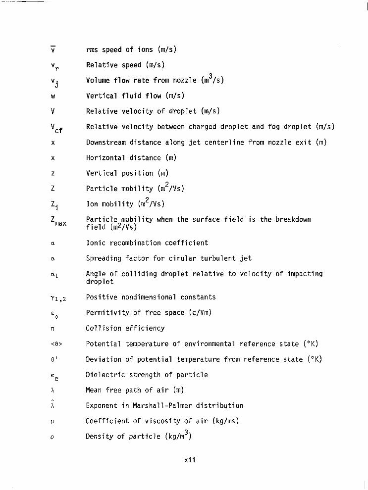
rms speed of ions (m/s)
Relative speed (m/s)
Volume flow rate from nozzle (m3/s)
Vertical fluid flow (m/s)
Relative velocity of droplet (m/s)
Relative velocity between charged droplet and fog droplet (m/s)
Downstream distance along jet centerline from nozzle exit (m)
Horizontal distance (m)
Vertical position (m)
Particle mobility (m2/Vs)
Ion mobility (m2/Vs)
Particle mobility when the surface field is the breakdown field (mz/Vs)
Ionic recombination coefficient
Spreading factor for cirular turbulent jet
Angle of colliding droplet relative to velocity of impacting droplet
Positive nondimensional constants
Permitivity of free space (c/Vm)
Collision efficiency
Potential temperature of environmental reference state (OK)
Deviation of potential temperature from reference state (OK)
Dielectric strength of particle
Mean free path of air (m)
Exponent in Marshall-Palmer distribution
Coefficient of viscosity of air (kg/ms)
Density of particle (kg/m3)
xii

'a
'e
PT
<P'
pW
T
9'
+e
Density of air (kg/m3)
Charge density (c/m3)
Total charge density (c/m3)
Density of the environmental reference state (kg/m3)
Density of water (kg/m3)
Acceleration time constant of particle (s)
Entropy (J/kg K)
Electrical potential (V)
JI Streamline (s-l)
w Vorticity (kg/m3s)
Subscripts
C Designates charged droplet
f Designates fog droplet
P Designates precipitating droplet
X Component in x direction
z Component in z direction
Supercripts
PO1 Denotes polarization
coal Denotes coalescence
xiii

1.0, INTRODUCTION
Charged particle techniques hold.promise for dispersing warm fog in
the terminal area of commercial airports. A survey of research relative
to this technique and a discussion of competitive techniques such as
thermal air, etc.,is given in Christensen and Frost [l-l]. The present
report focuses on features of the technique which require further study.
The physical principles upon which the technique is based and the major
experiments carried out in the past towards verification of the tech-
nique are described in Section 2.0. The futidamentals of the nozzle
operation are given in Section 3.0. A complete discussion of the char-
acteristics of the nozzle and the theory of particle charging internally
in the nozzle are described. Information from the extensive literature
on electrostatic precipitation relative to environmental pollution
control is incorporated into this discussion. The section ends with a
description of some of the preliminary and simplified analyses reported
in the literature on the jet characteristics and its interaction with
neighboring jets.
From the survey reported in Reference [l-l], it is evident that
much needs to be learned relative to the interaction of the charged
particles expelled by the nozzle and the fog droplets. The mechanisms of
charge transfer, coalescence, etc.,are somewhat understood by cloud physicists [l-2, l-31, but this understanding has not
been applied to the problem in hand. Also, since the charged particles
themselves result in the formation of the atmospheric electric field
which causes the charged fog droplets to be driven to the ground, the
physical process is highly dynamic. Modeling of the above-described
fog and jet interaction would be useful to optimize the nozzle design;
however, it is believed that the state of the art is such that an effec-
tive nozzle can be designed [l-4, l-51 and the effectiveness of the fog
dispersal technique evaluated experimentally. An understanding of the
basic unsolved equations governing the process is useful, however, to
interpreting the experimental results; therefore, Section 4.0 presents

the equation governing the transfer of water substances and of electrical
charge. A brief description of several semi-empirical, mathematical
expressions necessary as input to the governing equations is given. A
solution technique and the formulation of boundary conditions to ana-
lyzing the jet interaction with fog and the formation of the electric
field requires further development.
Section 5.0 describes the necessary ingredients of a field experi-
ment to verify the system once a prototype is built. The necessary
equipment, number of nozzles, accuracy of the instruments, parameters to
be measured, etc.,are discussed based on the extent of our existing
knowledge. The purpose of Section 5.0 is to provide insight as to the
magnitude of the field program necessary to verify the fog dispersal
system.
References
l-l. Christensen, L. S., and W. Frost. "Fog Dispersion," NASA CR 3255, March 1980.
l-2. Mason, B. J. The Physics of Clouds. New York: Oxford University Press, 1971.
l-3. Chalmers, J. A. Atmospheric Electricity. New York: Pergamon Press, 1967.
l-4. Willke, T. L. "Current Production in a Cylindrical Geometry Electrofluid D.ynamic Generator," U.S. Air Force, Aerospace Research Laboratories, Report No. ARL 71-0245, October 1971.
l-5. Lawson, M. 0. "Ion Generation by Corona Discharge for Electro- Fluid Dynamic Energy Conversion Processes," U.S. Air Force, Aero- space Research Laboratories, Report No. ARL 64-76, October 1964.

2.0 CHARGED PARTICLE FOG DISPERSAL CONCEPT
AND BACKGROUND RESEARCH
The concept of fog dispersal by charged particle techniques stems
from existing evidence that electric forces have profound effect on the
growth of water droplets in warm clouds and in fogs by collision and
coalescence. Carroz, et al. [2-l] and Cachet [2-2) have shown theoret-
ically that highly charged droplets possess much larger collection
efficiencies than similar but uncharged droplets. Also, the successful
introduction of large quantities of highly charged droplets into confined
regions of fog results in the generation of a substantial electric
field, which modify the natural fog over regions beyond the immediate
influence of charged materials. A general consensus [2-2, 2-31 indicates
that electric fields greater than 20 kV/m are required to influence
significantly the stability of a natural fog; and while there may be
considerable difficulty in engineering these large electric fields, the
potential rewards from an aviation operational point of view are large
enough to warrant further investigation.
Gourdine Systems, Inc., [2-41 appear to be the first to propose a
system having practical application for fog dispersal at airports.
Their concept involved using a matrix of charged particle spray guns
installed along and around an airport runway to propel charged water
droplets into the fog. An electric charge was thereby imparted to the
fog droplets, causing them to precipitate to the ground under the action
of space charged induced electric fields or through enhanced coalescence
and precipitation under gravitational forces. Application of this
concept calls for the development of a charged particle spray gun which
must charge the particles (charged carriers) internally and propel the
particles to the necessary heights to affect the clearing which allows
aircraft operations to continue. Secondly, to provide the optimum spray
gun design and matrix array for efficient warm fog dispersal, the charged
particle/fog droplet interaction must be understood. In particular, the
extent and intensity of the electric field which can be generated under
various climatic conditions, i.e., wind, fog density, turbulence, etc.,
must be known. The mechanism of transferring charge to the fog droplets
and of their following the electric field to ground, as well as the
mechanism of coalescence which enhances droplet growth and their migra-
tion to the ground by gravitational forces is not understood. In view
of the experimental and analytical difficulties which must be overcome
to develop a comprehensive model of this mechanism it is recommended
that a systematic development and testing of a prototype system be
carried out. The effectiveness and economic viability of this system
can be established in this manner without a complete knowledge of the
charged particle interactions.
The principle upon which a charged particle spray gun operates is
illustrated in Figure 2.1. Figure 2.la illustrates the principle of an
electrical gas dynamics direct energy conversion nozzle. A gas contain-
ing uncharged particles flows through a corona discharge and down a
dielectric channel. In the corona region molecular ions are injected
into the flow and some of these ions attach to the water droplets and
are swept downstream. The particles are discharged to a sharp, pointed
electrode collector downstream and the current passes through an external
resistance. Thus, energy in the flowing gas is converted to high-voltage
electrical energy. That is, the energy lost while flowing from the
ionizer, corona discharge region, to the collector appears as electric
energy, or heat, in the external resistance.
In the fog dispersal mode the collecting electrode is eliminated
and the charged particles are carried into the atmosphere by the flow
energy. Thus, kinetic energy of the flowing gas and particles is con-
verted into electric potential energy in the form of a large cloud of
highly charged particles. Since the charged particles dispersed to the
atmosphere find their way back to ground potential through the atmo-
sphere, the air becomes the external resistance, dissipating electrical
energy as heat through collisions between the air molecules and the
charged particles. The larger the size cloud of charges the longer the
path to ground and the larger the external resistance. For a given
current output, the larger the external resistance the larger are the
voltage and power that must be generated to maintain the charged cloud.
4

CORONA IONIZER -
OUT - EXTERNAL RESISTANCE
a) Energy mode.
I ‘CORONA IONIZER 4n
/-
0.. a
a
- AIR FORMS EXTERNAL RESISTANCE r-m
I -I- -
b) Fog dispersal mode.
Figure 2.1 Principle of charged particle fog dispersal technique [Z-4] *
5

Therefore, in order to establish a cloud of charged fog droplets of the
same polarity, a charged particle spray gun must raise the charges to a
high electrical potential energy with respect to ground, typically several
thousand volts, and propel these charged particles to sufficient heights
to affect fog clearing.
The initial spray gun used by Gourdine Systems, Inc. [2-41 used a
high-speed jet of air to carry the charged submicron water droplets into
the fog. The jet of air along with turbulent diffusion pushes the
charged particles to a height which preliminary experiments and calcula-
tions suggest can be on the order of 30 m. Continuous injection of the
charged water droplets from the spray guns maintains a constant space
charge electric field. The fog particles having acquired a charge from
interaction with the charge carriers are then considered to follow the
electric field and precipitate to the ground. A mathematical model of
this mechanism is given in later sections.
To test this system a laboratory and a field study were carried
out. A complete description of these studies is given in References
[2-5] and [2-6j. A summary of a full-scale field study, conducted in
the Panama Canal Zone [2-71, is given in the following sections to
provide the reader with an understanding of the practical approach to
warm fog dispersal and to familiarize him with the limited background
information available.
2.1 Summary of the Full-Scale Field Experiment in the Panama Canal Zone
A description of the experimental apparatus utilized in the Panama
Canal Zone full-scale field experiment as detailed in References [2-41
and [2-71 is given along with some of the estimated and measured charac-
teristics of the system. Also, the reported results of the experiment
are summarized.
In the Panama experiment, sixteen spray guns were set up in a 4x4
array with 38.1 m (125 ft) separation between guns. Figure 2.2 schemat-
ically illustrates this array and the location of the major fog monitor-
ing instrumentation sites. The meteorological van containing most of
the instrumentation was located some distance from the array to avoid
the possibility of distortion of results by grounding effects of the
metal tower. TWO visibility monitoring stations were utilized: the
b

0 EGD Spray Gun System
38.1 (125
J 38.1 m
(125 ft)
1
south Mobile Videograph
'f"t,
-a
0
0
0 I 1 kw, 115 V AC Portable Gasoline Generator
-Prevailing Wind
0
0
0
0
114.4 m (375 ft)
0
a
I I Meteorological Van
lxl North Stationary
Videograph
Figure 2.2 Panama Canal Zone field experiment arrangement [Z-7].
7

south mobile videograph and the north stationary videograph. In all
cases, reported data were measured with the south mobile videograph.
During the test period, ten field tests were carried out. Of
these, 40 percent of the experiments produced some effect on surface
visibility. These effects are discussed subsequently.
Space charge distribution measurements were made during only two of
the runs. These measurements indicated the existence of charged particles
at an altitude of at least 30.5 m (100 ft) and of the right order of mag-
nitude (-3 x 10m7 c/m3) corresponding to approximately 15 x lo6 V at a
height of 30.5 m (100 ft) [2-41. Data at the center of the array,
however, shows a factor of three less than expected, and the space
charge distribution according to measurements was, in general, nonuniform.
Electric field distribution measurements were made during all tests
to provide an indirect measurement of the relative distribution of
ground current density. Measurements indicated a field strength of
-4 x lo4 V/m at a distance of 77.8 m (255 ft) downwind of the test
array. Figure 2.3 from Reference [2-41 summarizes the time and space
relationship mapping of the electric field distribution.
2.1.1 Description of Experimental Apparatus
A charged particle spray gun in operation is illustrated in Figure
2.4 [2-71. The system consists of a nozzle or spray gun, a supply and
control hand cart, and a gasoline-driven air compressor. Sixteen of
these units were constructed and used in the experimental program.
Charged particle spray gun. A schematic of the spray gun nozzle is
shown in Figure 2.5. The major dimensions and working principles are
illustrated. A stream of saturated compressed air enters the spray gun
and passes through a nozzle as illustrated in Figure 2.5. The air
expands to supersonic conditions, cooling sufficiently to form droplets
of water. As the droplets pass through the corona discharge region of
the nozzle, they acquire a charge. The charged particles are then
carried by supersonic airflow down the dielectric channel and exhaust to
the atmosphere forming the space-charged cloud.
The operating characteristics of the spray guns utilized in the
Panama experiment, as reported in Reference [2-41, are given in Table 2.1.
8

r
X EGD Spray Gun
0 6 ft Circle
I 0 Center of each four spray guns. Top number, scanner faces X. Bottom number, scanner I faces away from X. Number in ( ) indicates 1
I time in hours. Midway measurement omitted
2.3 x 10' 2.8 x lo5
2.3 x lo5 1.5 x lo5
4 x lo4 0
(0340)
2.5 x lo5 1.5 x lo5
1.5 x lo5 1.0 x lo5
d= 0 3.8 x lo4
85 yds (0328) *
4 x lo4
2.8 x lo5 2.4 x lo5
2.0 x lo5 1.4 x lo5
0 3.0 x lo4 (0255)
2.5 x lo5 2.6 x lo5
2.0 x lo5 1.5 x lo5
Date: 11/23/72
V-G-6D
Background, +3.5 x lo3 V/m (0245)
1.8 x lo5
1.0 x lo5
0
@ 2.0 x lo5
1.0 x lo5
0 2.8 x lo4
(0325)
63)
2.5 x lo5
1.5 x lo5
2.5 x lo5
1.8 x lo5
0 4 x lo4
(0337)
0 2.5 x lo5
1.5 x lo5
0 2.0 x lo4
(0323)
63 3.0 x lo5
1.8 x lo5
a 2.8 x lo4 (0317)
3.0 x lo5 v/m
1.4 x lo5 v/m
Figure 2.3 Typical electric field mapping (relative ground-current density distribution) as reported in Reference [2-41.
9

Figure 2.4 Charged particle spray gun in operation [2-71.

DIA
0.320” DIA /
9-I-l
iNEEDLE HIGH VOLTAGE DC POWER SUPPLY LOCATED ON THE SUPPLY AND = CONTROL HAND u CART ::
Figure 2.5 Schematic of spray gun nozzle [2-41.
TABLE 2.1 Operating Characteristics of Spray Gun Used in Panama Experiment [2-41.
AIR-WATER .-- MIXTURE
Ionizer voltage 9 s 10 kv
I Compressor line pressure I 75 psig
I Volumetric flow rate of air I 50 scfm
Water consumption 38 cc/min, or 6.34 x 10⁻⁴ kg/s
r Short-circuited current 100 Q 135 x 10-C A I
70 ,-t, 80 kV
r- Mach number
r- Charge/mass ratio*
i- Droplet radius**
I Droplet charge
I 1.35 I
I 0.213 c/kg I
I 10-7 m I
8.92 x lo-19 c
Droplet mobility 5.7 x 10 -8 m2/Vs
*Charge/droplet -- = Short-Circuited Current A Mass/Droplet --W%t~o~s6ip~n--(%g/s ---P
**Derived from experimental charge/mass ratio and by using diffusion charging mechanism for particles in a supersonic channel.
11
The method of measuring the load voltage and the short-circuited current
are illustrated in Figure 2.6. Optimum outputs were achieved by adjust-
ing simultaneously the air/water mixture and the high voltage applied to
the ionizer.
As described in Section 3.0, one drawback to this type of spray gun
nozzle, identified by the present authors, is that the particles do not
remain in the corona region sufficiently long to become fully charged.
As will be shown, the time required to fully charge a particle is on the
order of milliseconds whereas at sonic speeds the droplets pass through
the corona region in microseconds.
Auxiliary equipment. The other components making up the system are
illustrated in Figure 2.7. All supplies, controls, and regulators
necessary to operate this spray gun were mounted on a mobile hand cart.
A water tank with all controls and regulators was mounted in the front
and a high-voltage DC power supply with a 110 AC volt input supplied
from a portable gas-driven generator along with a stand for the charged
particle spray gun were mounted in the rear. An electrical power
distribution network was employed to provide power to all 16 mobile.
units from the centrally located gas-driven generator.
Air provided by a portable air compressor entered the system at the
water tank inlet. The air pressure was controlled by a regulator and
fed through an on/off valve to the water tank. Pressurized water
entered a capillary tube in the water tank, passed through a flow meter
and through a capillary coil where it was mixed with a second air supply.
Mixing of the compressed air and water took place in a section of pres-
sure hose, and the air/water mixture was supplied to the charged particle
spray gun. The required water flow rate was controlled by adjusting the
metering valve on the flow meter.
2.1.2 Parameters Measured and Instrumentation
The parameters measured during the field program were:
l Atmospheric transmissivity (visibility versus time)
l Wind speed and direction versus time
12

0
8 C f /
SPRAY GUN
\
, SPRAY GUN STAND
f 0
COROU4 TIP
L maNI CLIP
SK)RT-CIRCUITED CmRENl MASLRMNT
Figure 2.6 Illustrates measurement of load voltage and of short-circuited current [2-41.

WATER TANK WATER TANK AIR PRESSURE GAUZE EGD SPRAY GW
I- AIR INLET
WATER TANK /
Al R REGULATO
AIR-WATER MIXTURE
LAIR-WATER MIXTURE ON/OFF VALVE
-CAPILLARY COIL (*TER):
SAFETY VALVE
\_FLOW METER WITH METERING VALVE
WATER OUTLET W/OFF VALVE
WATER TANK
\_ceiPlLLARY TUBE (WIlH 11’1” CL-E
TO BOTTOH OF WATER TANK)
QUICK DISCDMECT STRAP
QuiCK DISCOM4ECT STRAPS
EGD SPRAY GUN STAM
WATER-TIGHT, HIGH-MLTAGE, DC PQ,,ER SUPPLY KxlSiNt WITH DOOR REH3MD TO Sb0W CONTROLS AN) INSTRWS
FRCNT VIEW OF SUPPLY AN) CONTROL CAJ7T REAR “,Ew OF SUPPLY SN) CONTROL CART
Figure 2.7 Schematic of charged particle spray gun unit used in Panama experiment [2-41.

r -
l Fog drop size distribution and concentration versus time and altitude
o Atmospheric temperature and dew point, or relative humidity versus time
l Atmospheric electrical potential gradient versus time
l Atmospheric space-charge distribution versus time and altitude
o Ground-current density distribution versus time
Space-charge density distribution. A space-charge density probe
supported by a balloon-borne platform was used to measure the space-
charge density distribution. Details of the probe are given in Reference
[2-41. It consisted mainly of an aluminum cylinder with a spherical
brass ball centered axially in the middle. The ball was connected to
the input of an electrometer and the cylinder was electrically grounded.
The potential measured in the space-charge cloud is in direct proportion
to the space-charge density and the diameter of the cylinder squared.
The output of the probe was telemetered to a ground receiver.
Ground-current density distribution. The ground current density
distribution was measured indirectly by mapping the electric field as
obtained by a portable electric field scanner. The ground current
density was then estimated from the electric field map and the measured
space-charge density distribution. To determine an absolute distribu-
tion of ground-current density, the mobility of the charged particles
must be known.
Visibility. Visibility was measured with videographs located as
illustrated in Figure 2.2. The videograph, a product of Sperry-Rand,
Ltd., operates on measurement of backscattered light.
Fog drop size distribution and concentration. Fog drops were
collected on hand-held gelatin-coated slides.
Other climatological parameters. Temperature, dew point, wind
direction and speed were measured from a 15.2 m (50 ft) instrumented tower.
The meteorological van and tower were located somewhat out of the spray
gun array to avoid distortion of the electrical field resulting from
grounding effects of the metal tower. Measurements of temperature and
15

relative humidity were recorded at ground level while wind direction and
speed were recorded from sensors on the instrumented tower installed at
an altitude 15.9 m (52 ft) above ground level. Time is recorded in
local standard time and visibility in nautical miles.
2.2 Test Results
This section summarizes the test results as presented in Reference
[2-71. Ten fog dispersal tests were performed. Two of the ten tests
conducted were not evaluated because of equipment malfunction and prema-
ture breakup of the natural fog. Figure 2.8 reproduced from Reference
[2-71 summarizes results of the remaining eight dispersal tests. All
visibilities were recorded by the south mobile videograph and are
expressed in nautical miles (NMI).
November 16--Tests V-G(2) and V-G(3). In test V-G(2) the spray
guns were turned on at approximately 0435. With the exception of a
slight pulse at the beginning of the tests, visibility averaged 0.2 NMI.
Sixty minutes after spraying began the visibility increased steadily
reaching a peak of 3.9 NM1 8 min after spraying was terminated at 0545.
Visibility then decreased abruptly to near its original value in approxi-
mately 4 min. Temperature and relative humidity remained constant at 75"
F and 100 percent, respectively, during the test. Winds were recorded
calm throughout the test period with a slight southerly drift in fog
being noted.
Test V-G(3) was a continuation of test V-G(2). Here the spray guns
were activated at 0615 and continued to operate until 0645. Wind speed
was recorded as calm except for a brief 2-minute period of 2 to 4 kts
at 0630. The prevailing wind direction during the test was equally
divided between WSW (250 deg) and NW (315 deg). Visibility initially at
0.2 NM1 improved reaching a peak of 0.8 NM1 in 22 min from activating
the spray guns. Following spray termination a steady decreasing trend
in visibility was recorded.
Visual observers indicated that the sky was totally obscured
throughout V-G(2) and V-G(3). Temperature increased from 75' F to 76" F,
and relative humidity decreased from 100 percent to 97 percent during
this test period. 16
4.0- --
Charged'Water Spray I
zi
E h .Z 2 2.0: -3 .i 3
30 60 90
Time (min)
a) Visibility plot--test V-G(Z).
t- Charged Water Spray --I
Figure 2.8 Test results of the Panama field experiment as reported in Reference [2-71.
17

0 30 60 90 120 150 180
Time (min)
c) Visibility plot--test V-G(4) and (5).
I- Charged Water Spray--
d) Visibility plot--test V-G(6).
Figure 2.8 (continued).
18

0 30 60 90 105
Time (min)
e) Visibility plot--test V-G(7).
30 60 60
Time (min) Time (min)
90 120 90 120
f) Visibility plot--test V-G(9). f) Visibility plot--test V-G(9).
Figure 2.8 (continued).
19

4.
0.
.O-
/-Uncharged{- + Uncharged -1 Water Spray I Water Spray
0:
- ~~‘,l,,‘,,,,l~,~,l,,,,l,,,~~,,ll~~~’,~~~’~~,,l,,~,l,,,,l,,,,l,,,,‘~~~,l~~~~ll~~~l~~~~‘~~~~
0 30 60 90 120
Time (min)
g) Visibility plot--test V-G(10).
Figure 2.8 (concluded).
November 18--Tests V-G(4) and V-G(5). Spray guns were operated
from 0400 to 0500 for V-G(4) and from 0530 to 0630 for V-G(5). Both the
south and north videograph plots showed poor visibility throughout both
test periods. Wind speed varied from 1 to 5 kts during V-G(4), dimin-
ished to calm except for a 20-minute period of 1 to 3 kts from 0550 to
0610 during V-G(5). The prevailing wind direction during test V-G(4)
was WNW (295 deg). This direction held during the first half of test
V-G(5) becoming WSW (240 deg) during the second half. It should be noted
that in both cases the wind was such as to carry the cleared fog patch
away from either of the videograph systems.
Temperature and relative humidity were constant at 74" F and 100
percent, respectively, throughout both test periods.
Sky conditions were partially obscured with stars intermittently
visible during test V-G(4), becoming totally obscure during test V-G(5).
November 23--Tests V-G(6) and V-G(7.). Spraying began for test
V-G(6) at 0255 and was terminated at 0400. Visibility was recorded at
0.1 NM1 as spraying began. A clearing pulse peaking at 0.4 NM1 occurred
20

20 min after spraying began and a second pulse peaking at 0.7 NM1
occurred 24 mi-n later. Visibility stabilized at 0.1 to 0.2 NM1 after the spraying was terminated.
Stars were visible though partially obscured throughout the test
period.
For test V-G(7) the spray system was activated from 0445 to 0520.
Uncharged water was used until 0500 and charged water was used the
remainder of the time. Winds were calm with a slight southerly drift
of the fog.
A visibility pulse having a peak of 1.8 NM1 10 min after uncharged
spraying began, and a second pulse peaking at 1.2 NM1 1 min after charged
spraying began occurred. A third major clearing trend began as the
treatment was terminated, reaching a peak of 4.1 NM1 16 min after spray-
ing ended. Visual observations reflected these trends.
November 24--Tests V-G(9) and V-G(10). For test V-G(9) the spray
system was activated at 0245 and continued for one hour. Winds were
calm to slight with direction W (270 deg) to N (360 deg) during periods
of slight (less than 2 kts winds). Visibility remained at approximately
0.3 NM1 during the first 48 min of treatment after which a significant
clearing pulse peaking at 1.8 NM1 occurred followed by a decline to
nearer the original value as spraying was terminated.
As shown in the figure, both charged and uncharged spraying was
utilized for test V-G(10). Winds during the test period remained
uncharged from V-G(9), continuing calm to slight. Uncharged water
spraying began at 0415, and at approximately 0430 charged spraying was
initiated and continued for 35 min. Five minutes after charged spraying
was initiated, a gradual increasing trend in visibility began. Nineteen
minutes after the charged spraying began a sharp increase in visibility
occurred peaking at 3.4 NM1 4 min later. An equally sharp decrease in
visibility occurred as charging was terminated. During the final
uncharged phase, visibility returned to its original value of approxi-
mately 0.2 NMI.
21

2.3 Reported Conclusions from the Field Tests
Of the ten fog dispersal field tests conducted in the Panama Canal
Zone, the conclusions reproduced from Reference [2-71 were:
1. Visibility improvement occurred during the treatment or treatment lag period in six out of eight test cases.
2. The magnitude and persistence of visibility improvement, as well as the treatment lag time to achieve such improve- ment, varied widely from case to case causing inconsistent results.
3. Under the test conditions that existed, the spray system was incapable of sustaining a fog clearing once it was achieved. Several times visibility improvement occurred during the treatment, only to deteriorate while treatment was still in progress. This failure may have been due to too strong a wind flow thus prohibiting cumulative effects.
4. Variation in wind flow and/or low-level air turbulence may have caused test distortion on the day treatment effects failed to occur.
5. Applying statistical visibility treatments (as described in Reference [2-7]), it was concluded that clearing effects were achieved on three of the four test days and in six out of eight test cases.
Conclusions drawn from the same tests by Reference [2-41 may be
summarized as follows.
1. The electric field and space-charge density were nonuniform in the field test.
2. The fog closed in after shutdown of the spray guns indi- cating that visibility improvements observed during spray gun operations were actually under persistent fog conditions.
3. The height to which the space charge was propelled by the spray guns was verified experimentally to be of 30.5 m (100 ft) minimum by the measurement of the space-charge density probe.
4. Instrumentation recorded fog clearings in general were obtained under favorable conditions of calm wind. Visual clearings were also observed under conditions of unfavor- able wind speed. Based on theoretical analysis [2-41, a moving fog of the order of 0.3 NMI/hr would mask the clear- ing effect of a 4x4 spray gun array as utilized in the Panama Canal experiment.
22
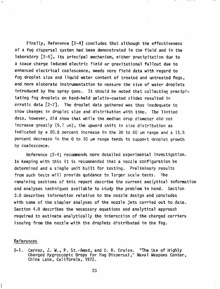
Finally, Reference [2-41 concludes that although the effectiveness
of a fog dispersal system had been demonstrated in the field and in the
laboratory [2-51, its principal mechanism, either precipitation due to
a space charge induced electric field or gravitational fallout due to
enhanced electrical coalescence, needs more field data with regard to
fog droplet size and liquid water content of treated and untreated fogs,
and more elaborate instrumentation to measure the size of water droplets
introduced by the spray guns. It should be noted that collecting precipi-
tating fog droplets on hand-held gelatin-coated slides resulted in
erratic data [2-71. The droplet data gathered was thus inadequate to
show changes in droplet size and distribution with time. The limited
data, however, did show that while the median drop diameter did not
increase greatly (5.1 pm), the upward shift in size distribution as
indicated by a 20.6 percent increase in the 30 to 60 urn range and a 15.5
percent decrease in the 0 to 30 urn range tends to support droplet growth
by coalescence.
Reference [2-41 recommends more detailed experimental investigation.
In keeping with this it is recommended that a nozzle configuration be
determined and a single unit built for testing. Preliminary results
from such tests will provide quidance to larger scale tests. The
remaining sections of this report describe the current analytical information
and analyses techniques available to study the problem in hand. Section
3.0 describes information relative to the nozzle design and concludes
with some of the simpler analyses of the nozzle jets carried out to date.
Section 4.0 describes the necessary equations and analytical approach
required to estimate analytically the interaction of the charged carriers
issuing from the nozzle with the droplets distributed in the fog.
References
2-1. Carroz, 3. W., P. St.-Amad, and D. R. Cruise. "The Use of Highly Charged Hygroscopic Drops for Fog Dispersal," Naval Weapons Center, China Lake, California, 1972.
23

. . _
2-2. Cachet, R. "Evolution d'une Gouttelette d'eau Chargee dans un Nuage on un Brouillard a Temperature Positive," ACAD (Paris) COMPT REND, Vol. 233, 1951, p. 190.
2-3. Moore, C. B., and B. Vonnegut. "Estimates of Raindrop Collection Efficiencies in Electrified Clouds," American Geophysics Union, Geophysical Monograph No. 5, 1960, pp. 291-304.
2-4. Chiang, T. K. "Field Evaluation of an Electrogasdynamic Fog Dispersal Concept," Part I, FAA-RD-73-33, February 1973.
2-5. Jiusto, J. E. "Laboratory Evaluation of an Electrogasdynamic Fog Dispersal Concept," FAA-RD-72-99, 1972.
2-6. Chiang, T. K., and M. C. Gourdine. "Electrogasdynamic Fog Dispersal Test and Evaluation for a Ground-Based System," Internal report for 'FAA by Gourdine Systems, Inc., Livingston, New Jersey, January 1973.
2-7. Wright, T., and R. Clark. "Field Evaluation of an Electrogasdynamic Fog Dispersal Concept," Part II, FAA-RD-73-33, February 1973.
24

3.0 NOZZLE CHARACTERISTICS __---_--------
This section describes the fundamentals of the nozzle operation.
A discussion of the characteristics of the nozzle and the theory of
particle charging internally within the nozzle is described. The exten-
sive literature on electrostatic precipitation techniques available in
the environmental pollution literature is incorporated into the discus-
sion. A description of some of the preliminary and simplified analyses
reported in the literature on the jet characteristics and its interaction
with neighboring jets concludes Section 3.0.
3.1 Particle Charging in a Corona Discharge
The charged particle fog dispersal technique (CPFDT) requires a
high current source of unipolarity charged particles. This is currently
provided by passing a high-speed saturated airstream through a corona
discharge (see Figure 3.1) [3-l through 3-61. An understanding of the
operation of the CPFDT requires a detailed examination of the corona
discharge and the charge transfer that occurs in the corona discharge
region.
A corona discharge occurs in a high pressure gas when a high
voltage is applied between a small wire or other form of electrode with
a very small radius of curvature and a large grounded electrode which
surrounds the wire (Figure 3.2). A very high electric field occurs near
the wire which accelerates any free electrons which are present, causing
them to produce additional electrons upon impact with neighboring gas
molecules. This initiates an avalanche which produces large quantities
of electrons and positive ions near the wire. The highly mobile elec-
trons quickly move toward the grounded electrode and into a region of
smaller electric field where they can no longer generate additional
electrons. If electronegative molecules, such as 02, C02, or H20 are
present, then the electrons attach themselves to these molecules forming
stable ions. Because of their considerably smaller mobility, the ions
25

ar 4 Neutral
Particles
Ionizer I Power
SUPPlY '
l-
v -v-w
\ . . . . .
Corona Ionizer n n.
v @ Ionized - Particles
Wc o-+n+n+\\ -
Figure 3.1 Operating principle of charged particle fog dispersal technique [3-71.

Droplet
Form Negative Ions n
.rons
Free electrons
Region of Corona Glow
Electrons and Ions Formed in Region Close to Wire Where iS Very Large (Electronegative)
) E smaller so more electrons are not formed here. Electrons attach themselves to electronegative atoms (02, CO2, H20) to form stable ions which drift very slowly toward the positive electrode.
Figure 3.2 Physics of corona discharge [3-91.

drift only slowly toward the grounded electrode and a stable space
charge is formed in the region between the corona glow, which is close
to the wire, and the surrounding electrode.
If particles, such as water droplets, are passed through the space
charge, then it is possible for them to pick up charges from the ions.
The process of charging a water droplet is complicated, but it is common
practice to simplify the analysis of the general process and distinguish
two main processes, namely, field charging and diffusion charging [3-8,
3-9, 3-101. Field charging accurately describes the charging of particles
having a radius greater than 0.5 pm while diffusion charging is an
approximate description of the charging of particles having a radius
less than 0.2 urn [3-81. The charging of intermediate-sized particles
must be described by the combination of both types of charging [3-g].
In the following discussion, it is assumed that the particles are
spherical.
3.1.1 Field Charging
First, consider the field charging process. Let E, be the mean
electric field in the space charge region (lo5 to lo6 V/m). The electric
potential and flux lines surrounding an uncharged spherical particle
which is placed in this field are shown in Figure 3.3. If an ion is
brought in the neighborhood of the particle as a result of its motion in
the electric field, then an induced dipole is generated in the particle
and the ion is attracted to the particle (Figure 3.4). This process
continues (Figure 3.5) until a saturation charge is acquired on the
particle and all other charges are repelled (Figure 3.6). The particle
acquires charge according to the relation [3-81 (mks units are used
throughout the following sections)
n t -= n S t + to (3-l)
where ns is the saturation number of charges
“S
4re0EOa2 =K e
28
(3-2)

r- I II I I I 1
I, I . IllI\ \ I I
J-----L 1 Ill\ + ,--.k> ; ~+-+'r-"- -1
Ki ! il
I I * 81,’ I!!,I! i i I I I I!!! I , I I
Figure 3.3 Potential and flux lines around an uncharged spherical particle [3-9, 3-143.
Figure 3.4 Dipole induced in spherical particle due to presence of nearby charged particle [3-g].
29

-cq- ; I 1 I
i
Figure 3.5 Potential and field lines around a partially charged spherical particle [3-141.
Figure 3.6 Field lines around a fully charged spherical particle [3-g].
30
I

3; conducting particle K=
3K e Ice + 2 ; dielectric particle
and
4E to = Ni e"Zi
(3-2)
(3-3)
Ion mobilities, Zi, are of the order of 10 -4 m2/Vs (see Figure 3.14,
page 50, and Table 3.9, page 52) and the ion number density in the space
charge, Ni, is of the order of 1015 mm3. For water K = 2.93, but it
will be assumed to be equal to 3.0, for convenience, in the following
equations.
Using the numerical values for the physical constants, Equations
3-2 and 3-3 can be written as
n = 2 08 x 10' a2 E s * 0 (charges) (3-4)
2.21 x lo8 to= NZ
(s)
ii (3-5)
Calculated values are given in Tables 3.1 and 3.2. The electric field
at the surface of a spherical particle is given by
(3-6)
Es = 1.44 x lo-' n a2 (V/m)
Note that if the particle has a saturation charge, then (see Table 3.2)
Es = KE, = 3Eo (V/m> (3-7)
The charge is built up relatively slow and after 9t, has only reached 90
percent of the saturation charge (Figure 3.7). Thus, a particle will
have to remain in the space charge for a relatively long time to be able
to acquire maximum charge.
31
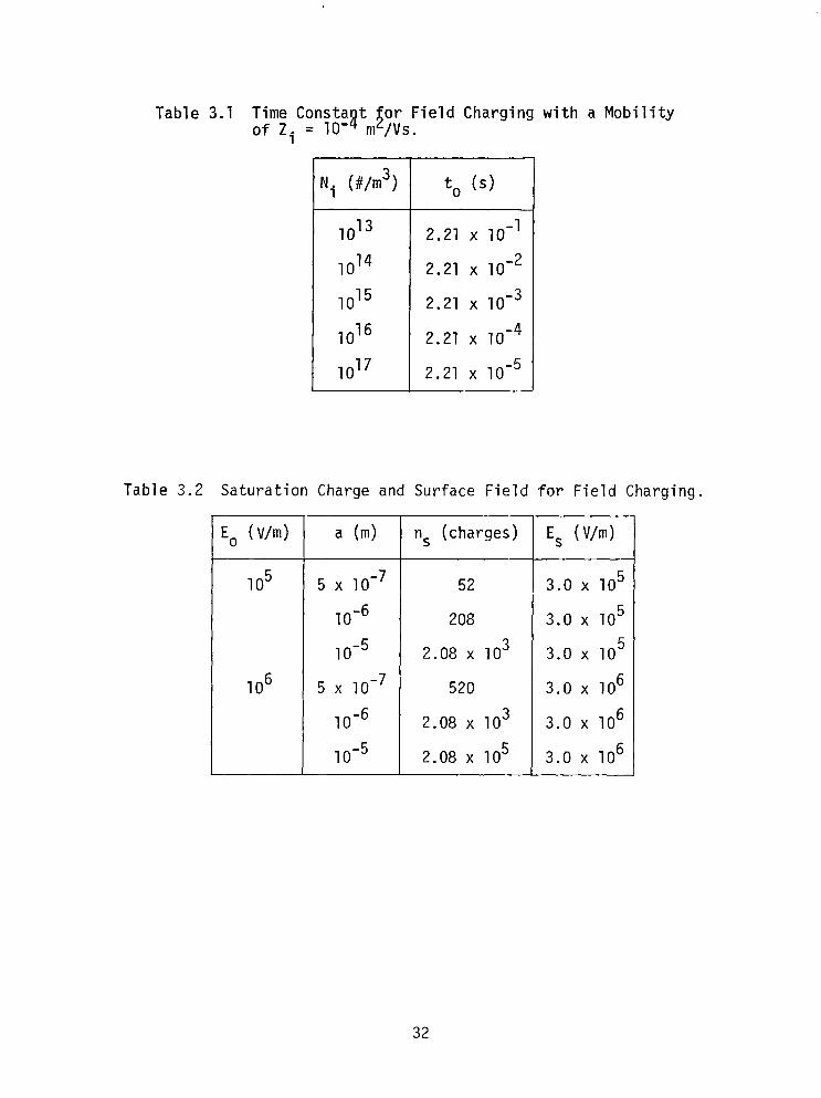
Table 3.1 ;Srn; Consta t or Field Charging with a Mobility
i = 10-g .$"s .
1014
1015
1o16
1017
2.21 x lo-2
2.21 x lo-3
2.21 x lo-4
2.21 x lo-5
Table 3.2 Saturation Charge and Surface Field for Field Charging.
E. (v/m)
lo5
106
a b-4 ns (charges)
5 x lo-7
lo-6
lo-5
5 x lo-7
lo-6
1o-5
52
208
2.08 x lo3
520
2.08 x lo3
2.08 x lo5
Es (V/m)
3.0 x lo5
3.0 x lo5
3.0 x lo5
3.0 x lo6
3.0 x lo6
3.0 x lo6
32

n/n S
1.0
0.5
0 0 10 20
Figure 3.7 Charge buildup for a field charged particle [3-g].
If the particles stay in the corona space charge region long enough
to acquire the saturation charge, then the maximum current that can
leave the nozzle is related to the nozzle particle mass flow rate. The
charge to mass ratio for particles of density, p, is given by
gEcJEo t !I=--- m ap I I t + to (3-8)
For water
(c/kg)
Written in terms of the particle surface field
3EOES 4=---- m a0 (3-g)
and for water
E ; = 2.66 x lo-l4 $ (c/kg) (3-10)
The surface field cannot be greater than 3 x lo6 V/m to prevent a corona
discharge [3-3, 3-10). Therefore, the charge to mass ratio has a maximum for a given particle size which increases with decreasing particle size
33

(Figure 3.8). Values of q/m for t much greater than to are given in
Table 3.3. Note that Equation 3-10 is valid for all size water droplets.
The particle can acquire charge until the electrical stresses are
greater than the surface stresses. If that occurs, then the particle
becomes unstable and loses mass and charge due to the Rayleigh insta-
bility. Instability occurs if
E; > s 02/m2) 0
or, for water at 20" C,
0.0001 0
Particle Diameter, D (w-4
Figure 3.8 Charge to mass ratio for sphzrical particles
.l 1.0 10 100 1000 10,000
in ai
34
(3-H)
r [3- .10].

Table 3.3 Charge to Mass Ratio for Field Charging.
Es ’ 1.81 x lo5
a l/2
E, (V/m> a (4
lo5 5 x lo-8
lo-7
5 x lo-7
lo6
1o-5
lo6 5 x lo-8
lo-7
5 x lo-7
1O-6
lo-5
(V/m)
q/m (c/kg)
0.159
7.97 x 10⁻²
1.59 x lo-2
7.97 x lo-3
7.97 x 1o-4
1.59
0.797
1.59 x 10-l
7.97 x 1o-2
7.97 x lo-3
(3-12)
Es will be equal to the maximum value 3 x lo6 V/m for a particle of
radius 3.6 x 10m3 m. This is much larger than any particles used in the
CPFDT and so the Rayleigh instability is not a limitation to the maximum
particle charge.
3.1.2 Diffusion Charging
Small particles (radius < 0.2 pm) collide with ions that are
brought in contact with them as a result of thermal diffusion. This
process was first examined by Arendt and Kallman [3-711 and simplified
by White [3-B]. The White expression for the number of charges acquired
by a particle as a function of time is given by
n 4ncoakT
= e2 ' 1
(charges) (3-13)
35

Assuming nitrogen ions at 300" K, this expression can be written as
n = 1.795 x lo7 a an(1 + 7.37 x 10m5 Niat) (charges) (3-14)
This expression is plotted in Figure 3.9.
Several differences should be noted between the two types of
charging processes. First, the diffusion charging expression is inde-
pendent of the electric field in the corona space charge, but this must
be considered to be an approximation, albeit an accurate one, for the
smaller particles. Second, a saturation charge does not exist for
diffusion charging. However, the particle can never acquire a charge
greater than that required to produce a breakdown field at the particle
surface (3 x lo6 V/m). The time to reach thebreakdown surface field is given
in Table 3.4. If the particles have acquired enough charge to achieve a
breakdown surface field of 3 x lo6 V/m, then the number of charges on
the particle is given by (Equation 3-6)
4lTC n= --A a2Es e
n = 2.08 x 10¹⁵ a2 (charges)
(3-15)
In the previously used nozzles (see Section 3.2) which had only a
single corona region through which the water droplets rapidly proceeded,
the particles were not in the corona region long enough to acquire
either the saturation charge for the field charged particles or to
approach the breakdown field for the diffusion charged particles.
Therefore, more charge could be emitted by passing the particles through
an extended corona region or multiple corona regions. Also, it is
apparent that smaller droplets can carry a relatively greater amount of charge
since the maximum possible charge to mass ratio (at breakdown field, for
example) increases as the droplet diameter decreases. Mobility consid-
erations, to be discussed later, indicate that there is probably an
optimum range of droplets sizes which will deliver the maximum charge to
the greatest heights in the fog.
36

N: = 1016/m3 I
-
V = 482 m/s
T = 298’ K
a = 0.05 urn
10 -5 1O-4 10-j lo-2
Charging Time(s)
Figure 3.9 Diffusion charging according to White's equation [3-B].
Table 3.4 Time to Reach Breakdown Surface Field (Ni = 1016/mm3).
a (4
lo-8
5 x lo-8
7 x lo-8
lo-7
2 x lo-7
t w 2.97 x 1o-4
8.90 x lO-3
6.51 x 10 -2
1.48
8.07 x lo4
3.1.3 Charqed Particle Mobility -.
For a system of moving charged particles in an electric field, z,
the current density, 5, is related to the fieid through the conductivity
of the media. In the present case, this relationship can be written as
s = P,Zi’ = pe; (3-16)
where Z is called the mobility of the charged particle of charge density,
pe, and ';; is the drift velocity of the particle in the field or the
velocity relative to the fluid. The mobility can be calculated once the drift velocity is known. Consider a spherical particle of charge, q,
initially at rest in a field, E. The field will accelerate the particle
in the field direction and its motion will be resisted by the fluid
dynamic drag. Assume that the particles are small enough so that the
Stokes' drag law is valid. This assumption will be examined later.
Then, the particle acceleration is described by the following equations,
assuming a negatively charged particle.
F D = 6ruav FE = qE
4 O- 4
E
38

dv m dt = qE - 6awv
v = +K[l - eetlT] = v* (1 - ewtlT]
vJr = qE _ neE -- 6apa 6npa
(3-17)
(3-18)
(3-19)
The charged particle is accelerated to its terminal velocity, v*, in
about 5~. For air at 20' C, the terminal velocity is given by
v” = 4.63 x 10¹⁶ F h/s > (3-20)
where E is the electric field surrounding the particle which has n
charges. Once the particle leaves the nozzle, the field is created by
the charge density itself. If the jet is modeled as a cylindrical region
of constant radius equal to the jet exit radius, R., and having a uniform 3
charge density, then the field created by the charges alone at the edge
of the jet is E = RjPe/2Eo: and at the edge of the jet
v* = 2.61 x lo5 Rj;en (3-21)
This value of v* is useful for understanding the electrostatic spreading
rate of the jet. To obtain a numerical value for v*, Equation 3-l or
3-13 must be used for the number of charges on the particle. First,
assume the particles are field charged and have achieved the saturation
charge. This assumption will yield the maximum v*. Then, if K = 3.0,
v” = 5.45 X 10⁴EoaRjpe (3-22)
Note that this same equation holds for diffusion charged particles which
have acquired the breakdown field at their surface. It is necessary to
keep in mind that E. is the mean electric field in the corona region
where the particles were charged while the accelerating field in the jet
is created by pe.
39

To be able to use this expression, it is necessary to have an
estimate of pe. Applying a one-dimensional control-volume analysis to
the jet and assuming that pe and Uj are uniform over the nozzle exit,
then the current leaving the jet is given by
3 =rs l tidA = / peGj l iidA = Rjpeuj (c/s) (3-23)
Values of Ij and uj as measured by Gourdine [3-21 are given in Table 3.5.
Equation 3-23 was used to calculate the pe values given in the table.
Using the maximum pe (for the small nozzle), values of v* were calcu-
lated and are given in Table 3.6. Gourdine estimated that the particle
radius in his nozzle was about 10 -7 m.
Table 3.5 Characteristics of Nozzles Used by Gourdine [3-21.
Radius, Rj (m)
Current (A) (E,(O) = lo6 V/m)
q/m (c/b)
Z (m2/Vs)
uj (m/s)
Vj (m3/s)*
Pe Wm3)*
Large
3.12 x lO-3
160 x lO-6
0.125
6 x lO-8
415
1.27 x lO-2
1.26 x lO-2
Medium
1.56 x 10⁻³
80 x lO-6
0.25
1.2 x lo-7
415
3.17 x lo-3
2.52 x lO-2
Small
1.0 x lo-3
51.3 x lo-6
0.392
1.9 x lo-7
415
1.3 x lo-3
3.95 x lo-2
*Calculated values.
Next, consider the terminal velocity for diffusion charged particles.
Rather than using Equation 3-13 for n, it is more meaningful to assume
that the particle has built-up charge so that the particle surface field
equals the breakdown field, i.e., Es = 3E, = 3 x lo6 V/m and then from
Equation 3-6
ne = 4=ooa2Es . = 3 34 x 10B4a2 (c) (3-24)
40

Table 3.6 Terminal Velocity for Particles in Small Jet.
I- E, (V/m) ___--
lo5
lo6
a (4 - 5 x lo-7
lO-6
lo-5
5 x lo-7
lo-6
lo-5
v* (m/s)
1.1 x lo-2
2.2 x lo-2
2.2 x 10-l
1.1 x 10-l
2.2 x 10-l
2.2
Re
1.0 x lo-3
2.9 x lo-3
2.9 x 10-l
1.0 x lo-2
2.9 x lo-2
2.9
Then the maximum terminal velocity at the edge of a cylindrical region
of uniform charge density is
v* = 5.45 x 10" Rjpea h/s > (3-25)
This expression gives a value for v * = 0.214 m/s for the large jet of
Gourdine [3-21.
For spherical water droplets moving in air, the acceleration time
constant, T, is given by
T = 1 21 x 107a2 . (s) (3-26)
Values are given in Table 3.7. Under most circumstances the acceleration
time constant is much smaller than the characteristic charging times
(see Table 3.1, page 32, and Table 3.4, page 38) and, therefore, the
particles can be assumed to be always moving at their terminal velocity
corresponding to the charge which they carry at the time. Then from
Equations 3-16 and 3-18 the mobility is defined as
z= &=e_ 6Tpa (3-27)
For a field charged particle
41

Table 3.7 Acceleration Time Constant for Water Droplets in Air.
a b-4 T. (9
lo-8 1.21 x lo-'
1o-7 1.21 x lo-7
lO-6 1.21 x lo-5
lO-5 1.21 x lo-3 _
Z = 9.65 x.10B7Eoa (m2/Vs 1
and for a diffusion charged particle
2sokT
' = 3pe tm 1
(3-28)
(3-29)
Z = 8.31 x 10" an[l + 7.37 x 10B5Niatm] (m2/Vs 1
where t, is the length of time the particle remained in the corona space
charge. If t, was long enough so that the particle has acquired the
breakdown field at its surface, then Equation 3-29 can be replaced by
2EoEsa z = 3U, max Es = 3 x lo6 V/m (3-30)
Z max = 0.965a (m2/Vs >
Note that Ruhnke [3-31 incorrectly gave the expression Z = lOa, and this
accounts for the order of magnitude difference between the mobility
estimates of Ruhnke and those ofGourdine [3-21.
Values of the mobility determined from Equation 3-28 for field
charge particles are shown in Figure 3.10 for t >> to and for diffusion
charged particles according to Equation 3-29 are shown in Figure 3.11.
42

lo-
:
"5 N
-I 10
,c 10 -
-6 10 -
3
I I I I I I I I
Ni = 1o14
a = 0.5 pm
E 0 = lo6 V/m
Z = 4.83 x 10 -7 2
m /vs max
Time (S)
Figure 3.10 Mobility of field charged particles as a function of time spent in a corona discharge.
43
10 -8
a = 0.01 pm
Time (S)
a) a = 0.01 urn.
Figure 3.11 Mobility of diffusion charged particles as a function of time spent in corona discharge.
44

10 -4 I
Time (s)
b) a = 0.05 pm.
Figure 3.11 (continued).
45

1o-7
10 -8
% N
10 -9
lo-lo
a= 0.1 urn
= 9.7 x 10 -8 2
zmax m / VE
Time (s)
c) a = 0.1 urn.
Figure 3.11 (continued).
46

In all cases the mobility increases as the length of time that the
particle remains in the corona region increases. The particles even-
tually can reach the breakdown field at their surface and reach Zmax
given by Equation 3-30. For most particles this is not expected to
occur with the previously used nozzles because the particles probably do
than low4 seconds in the corona (see Section 3.2). The
ious particle sizes at a fixed charging time.is shown in
not spend longer
mobility for var
Figure 3.12.
From this al nalysis it appears that it is desirable to design a
nozzle system that produces the smallest possible droplets, because the
charge to mass ratio increases for decreasing size. It would also be
desirable to keep the particles in the corona region long enough for
them to acquire the maximum possible charge and to design the corona
discharge with the maximum ion density. This would probably require a
modification of the previously used nozzles. Also, for a given electric field
the smaller the particle the smaller the mobility (see Equations 3-28 and
3-29) so that the particle should be able to proceed further into the fog.
However, an analysis of the turbulent jet, including the effects of turbulent
diffusion, will probably indicate that diffusive effects will be too great
for the smallest particles and thus an optimum size will exist. This
analysis remains to be performed.
It should be noted that the particle mobilities are much smaller
than electron or ion mobilities. The mobilities of electrons in gases
are of the order of 0.4 m2/Vs (Figure 3.13) and about 10 -4 m'/Vs for
ions (Figure 3.14 and Table 3.8). It is for this reason that the
particles can leave the corona region and proceed to great distances in
the jet before the electric field effects disperse them.
The equation for the mobility of the water droplet, Equation 3-27,
was derived assuming that the Stokes' drag law was valid. However, that is true only if the Reynolds number based on the sphere diameter is much
less than one. Assuming air, the droplet Reynolds number based on the
particle diameter is
2Pavra Re= Fr = 1.32 x 10⁵vra
47
(3-31)

10-
max
/
/
:
I' /
Ni E 1016 mm3 /' /
/
/'
Particle Radius (Urn)
Figure 3.12 Mobility for fixed charging time. 48

16,000
0
I I I I I I I I I
o Loeb
A Townsend and Bailey
I I I I I I I 0.2 0.4 0.6 0.8 1.0
E/p (v/cm mHq)
Figure 3.13 Electron mobility in hydrogen [3-151.
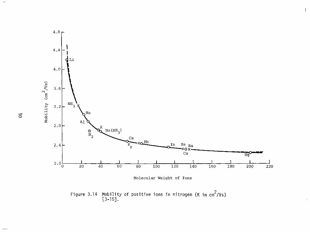
2.0( I I I I I I I I I I J 0 20 40 60 80 100 120 140 160 180 200 220
Molecular Weight of Ions
Figure 3.14 Mobility of positive ions in nitrogen (K in cm*/Vs) [3-151.

Table 3.8 Mobility of Singly Charged Gaseous Ions at 0" C and 760 mm Hg [3-151.
cm2/Vs
Z+
1.36
1.80
1.37
1.31
0.74
0.30
0.78
0.36
0.36
1.10
0.84
5.90
--- Gas Z-
Air (dry) 2.10
Air very pure 2.50
A 1.70
A very pure 206.00
c12 0.74
ccl4 0.31
C2H2 0.83
C2H5Cl 0.38
C2H50H 0.37
co 1.14
CO2 dry 0.98
H2 8.15
H2 very pure 7,900.oo
HCl 0.62
H20 at 100" C 0.95
H2S 0.56
He 6.30
He very pure 500.00
N2 1.84
N2 very pure 145.00
NH3 0.66
N2° 0.90
Ne we--
O2 1.80
so2 0.41
Z' = mobility of negative ion.
Z+ = mobility of positive ion.
----
0.53
1.10
0.62
5.09
5.09
1.27
1.28
0.56
0.82
9.90
1.31
0.41
1
51

where vr is the particle speed relative to the airspeed. Typical
Reynolds numbers are given in Table 3.6, page 41, assuming that the
particles are moving with v* through still air. For the sizes of
particles most likely to occur in the jets (less than 1 pm> the Reynolds
numbers are sufficiently small so that the Stokes' drag law is valid.
However, the particle diameters are so small that rarefraction effects
become important. The first rarefaction effect manifests itself as slip
over the surface. This results in a decrease in the drag compared to
the Stokes' drag. It is usual to apply the Cunningham correction factor
[3-141 to the continuum results previously given. The correction factor
is given in terms of the Knudsen number, which is defined as
Kn = x/a = 6.67 x 10v8/a (3-32)
where X is the mean free path length in air at standard conditions. The
Cunningham correction factor is
C= 1 + Kn(l.257 + 0.400 e -l.lO/Kn) (3-33)
Values are given in Table 3.9 and Figure 3.15. The previous results
must be corrected as follows. The particle drag is given by
F D = 6npav/C (3-34)
the terminal velocity becomes (see Equation 3-18)
Table 3.9 Knudsen Number and Cunningham Correction Factor.
a b-4 Kn = x/a C
lo-8 6.600 11.650
5 x lo-8 3.300 2.911
lo-7 0.660 1.890
2 x 1o-7 0.330 1.424
5 x lo-7 0.170 1.168
lo-6 0.066 1.084
52

:
12
10
8
6
1o-2 10-l
Particle Radius (pm)
loo
Figure 3.15 Cunningham correction factor.
53

v* = - neE c 6rva
(3-35)
the acceleration time constant becomes (see Equation 3-19)
(3-36)
and mobilities must be multiplied by C(Zcorr = ZC). This has a rather
substantial effect upon the magnitude of the mobility and its variation
with particle size. The mobilities given in Figure 3.12 are corrected
for rarefaction effects in Figure 3.16. At the higher ion densities
there is a noticeable minimum in the mobility curve. For those condi-
tions it would be desirable to choose particles whose radius places it
near the minimum. This type of behavior was predicted by Ruhnke [3-33
(see Figure 3.17) but does not always occur.
3.2 Previous Nozzles
Several nozzles have been used previously to test out the principles
of aerosol precipitation. These nozzles will be briefly described in
this section. At the end of the section desirable features of future
nozzles, based on the results of Section 3.1, will be discussed. The
previous nozzle did not incorporate these design features.
One of the earliest nozzles was designed by Whitby [3-41 to acceler-
ate ions. Ions which were generated in a corona near the needle were
accelerated through a sonic orifice (Figure 3.18). Output currents of
16 PA using 2.5 cfm of air at 30 psig through a one-sixteenth inch
orifice were achieved.
Ruhnke [3-31 analyzed the charge decay in a jet and constructed a
nozzle to check the calculations. A schematic of his apparatus, derived
from his written description, is shown in Figure 3.19. The charge in
the corona generated at the tip of the hypodermic needle was trans-
ferred to the fine mist of water droplets that was created. A space-
charge density of about 10e2 c/m3 was built up on the droplets before
breakdown occurred. The jet produced a current of about 15 PA, and the.
current could not be greatly increased without producing a corona
54

lr
lo-
';; mc 10-l
-5 N
10 -9
/ ,’ / 0 0
1o-L 10-l 10-O
Particle Radius (Pm)
Figure 3.16 Mobility for fixed charging time corrected for rarefraction effects.
55

1O-4
1O-5
10-E
-i 10
0 .OOl 0.01 0.1
Particle Radius (pm)
Figure 3.17 Expected variation of mobility with particle size [3-31.

A = lucite tube, B = end caps, C = end cap, D = orifice plate, d = orifice diameter E = needle positioning bracket,
I F = needle, G = needle stop, H = air connection,
s = needle spacing
Figure 3.18 Schematic of sonic jet ionizer [3-41.

Air, 20 psid-
1 / Hypodermic Needle
1 mm Diameter
Figure 3.19 Ruhnke charged droplet source [3-31.
discharge at the jet exit. Ruhnke estimated that the average mobility
of his droplets was about 10 4 m2/Vs .
The only field tests of jets of charged particles for warm fog
dispersal used nozzles designed by Gourdine [3-l, 3-2, 3-71. These
experiments were described in Section 3.1. Details of some of the
nozzles built by Gourdine are shown in Figures 3.20 and 2.5 (page 11).
Saturated air was expanded through a converging-diverging nozzle leaving
the nozzle at a Mach number of about 1.35. During the expansion
process, the saturated air became supersaturated and small water drop-
lets were formed. Near the throat region the droplets passed through a
corona region and acquired a charge.
Properties of the nozzles were given in Table 3.5, page 40.
Nozzle currents were up to 160 WA. The corona region was less than
3 x 1o-2 m long, and with a sonic speed of 360 m/s at the throat, the
droplets remained in the corona region of the Gourdine nozzle less than
8 x lO-5 s. Gourdine estimated that the droplets had a radius of about
0.1 pm. From Equation 3-10 the maximum charge to mass ratio for that
size particle is 0.8 c/kg. Measured values of charge to mass ratio were
much less (Table 3.5), and therefore it can be concluded that the
58

/-
Attractor
/I - Stand-Tubing - Stand-Tubing
EGD Spray Gun EGD Spray Gun
Ionizer Needle Ionizer Needle
Jet Section Connector
Figure 3.20 Gourdine nozzle [3-71.

particles did not remain in the corona region long enough to acquire the
maximum charge.
The following recommendations can be made concerning the design of
future nozzles:
1. The water particles should have a radius of about 0.1 pm to minimize the mobility.
2. The ion number density in the corona region should be as large as possible.
3. The water particles should remain in the corona region long enough to acquire the maximum charge to mass ratio. The last feature probably can best be achieved by allowing the droplets to pass through multiple corona discharges.
3.3 Models of Field External to Nozzle Exit
For the CPFDT to be useful the air jet must propel the charged
droplets to large heights (at least 50 m) and must create a large charge
density to that altitude. It is, therefore, important to develop
expressions for predicting both the decay of the charge density in the
jet as it proceeds upward and the charge density in the region exterior
to the jets. These charge number densities are labeled NJ and NBJ,
respectively, in Figure 3.21. Several approximate expressions for these
quantities have been derived and they will be given in this section. A
program for accurately determining the number density field plus the
remaining aspects of the fog dispersal problem will be outlined in the
next section.
Because of the relatively low charge densities within the jet, the
magnetic field created by the moving charged particles can be ignored.
Then only one of Maxwell's equations needs to be kept plus the equation
for charge conservation. The relevant equations which describe the
charge density in the jet are
v l i? = Pe/Eo (3-37)
ape at +'
J=(-J
;= p,zi + peT;
(3-38)
(3-39) 60

N BJ Between Jets
Ground
Figure 3.21 Schematic of multiple jet array.

- -. ..--. .- -- .- -- - --.--- .-...-- .--.. ..- - . . .._.
Many analyses can neglect the fluid dynamic velocity term. The results
given below all have used these equations as a starting point.
First, consider the analyses for the decay of the charge density in
the jet. Whitby [3-4) analyzed the charge number decay in a closed
space. He assumed that the particle charge and mobility were constant,
the space was not acted upon by fields, and that the particle number
density was uniform in space at all times. The number density decay was
found by integrating Equation 3-38 yielding the expression
1 1 + 4nNoneZt (3-40)
Noting that this expression is independent of geometry, it was then
applied to the charge number density decay in a jet by assuming that the
charge concentration is only a function of time since a given volume of
gas has left the corona region. Using the expression for the gas
velocity along the centerline of a circular turbulent jet (subsonic or
supersonic-- see Harsha [3-IZ]), u = b/x
X
u=;, t= s!f=g i 0
then the decay expression becomes
NJ -= 1
NJo 1 + 2nNJoneZx2
b
(3-41)
(3-42)
where NJ0 is the concentration at the jet exit. Measurements by Whitby
[3-41 of the decay of a unipolar ion beam confirmed the general correct-
ness of this expression.
Whitby [3-61 assumed that the charge number density outside the
region of the jet could be described as that which was generated by a
spherical source located some distance downstream from the nozzle exit.
Consider a spherical source, shown in the figure, where all properties
are functions only of the radial coordinate. Let Q be the total current
from the source.
62
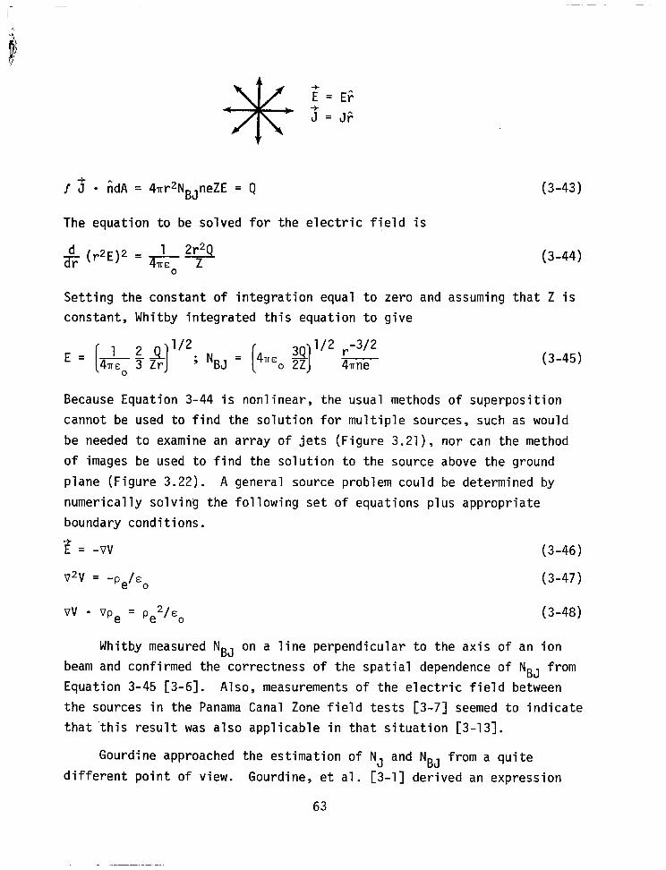
Z 3 l idA = 4nr2NBJneZE = Q (3-43)
The equation to be solved for the electric field is
& ($E)2 = &?$% 0
(3-44)
Setting the constant of integration equal to zero and assuming that Z is
constant, Whitby integrated this equation to give
E = [&;#2; NBJ = (4nco $'2 &2 (3-45)
Because Equation 3-44 is nonlinear, the usual methods of superposition
cannot be used to find the solution for multiple sources, such as would
be needed to examine an array of jets (Figure 3.21), nor can the method
of images be used to find the solution to the source above the ground
plane (Figure 3.22). A general source problem could be determined by
numerically solving the following set of equations plus appropriate
boundary conditions.
;i = -0v (3-46)
v2v = -pe/Eo (3-47)
vv l vpe = Pe2/Eo (3-48)
Whitby measured NBJ on a line perpendicular to the axis of an ion
beam and confirmed the correctness of the spatial dependence of NBJ from
Equation 3-45 [3-61. Also, measurements of the electric field between
the sources in the Panama Canal Zone field tests [3-71 seemed to indicate
that this result was also applicable in that situation [3-131.
Gourdfne approached the estimation of NJ and NBJ from a quite
different point of view. Gourdine, et al. [3-l] derived an expression
63

\\ Ground
\\ Ground
Figure 3.22 Single and multiple sources above ground plane.

for the conservation of charge from a circular turbulent jet by utilizing
the spreading rate of a turbulent jet [3-161
r = Rj + ax = Rj + 0.0848x (m) (3-49)
and assuming -that the electric field at the edge of the jet is equal to
that which exists at the edge of an infinitely long cylindrical region
of constant radius, R j, and constant uniform charge density, ne. Apply-
ing Gauss's law to such a region the field is given by
Rj
0 pe
r < R. - J
r > R. 3
Using this result, the charge density equation, as corrected by
Christensen and Frost [3-171 is
NJ --= -'
NJo
2ZE(o) R" + 2ZE(o)a: I 2 j 2
(3-50)
(3-51)
where E(o) is the electric field at the edge of the jet (r = Rj) at the
nozzle exit (x = 0). This expression is plotted, using the parameters
for the large nozzle used by Gourdine [3-21, in Figure 3.23. For these
parameters this equation predicts a much slower decay of the number
density than is predicted by Equation 3-42. There is no experimental
confirmation of this prediction.
For the charge number density between the jets Gourdine, et al.
[3-l] assumed that the turbulent jet entrainment would create a region
of uniform space charge between the jets in a large array, such as would
be used near an airport. This model should be contrasted to the spher-
ical source distribution which Whitby used to describe the charge density
between the jets (Equation 3-45). Gourdine assumed that the charge
density, pa, is constant to a height H where the jet charge density
equals the charge density in the surrounding atmosphere (i.e., H is
height where NBJ = NJ). Then the field and height are given by
65

10-
g B
b Z
10-
10-
R. 3 = 3.12 x 1OpJ m
U. 7 = 415 m/s
c. \ E(o) = 10" V/m \
z=8xlO -8 2
m /v ‘S
I I
0.1 1 10
Vertical Distance (m)
100
Figure 3.23 Charge number decay according to Gourdine expression [3-21.
66
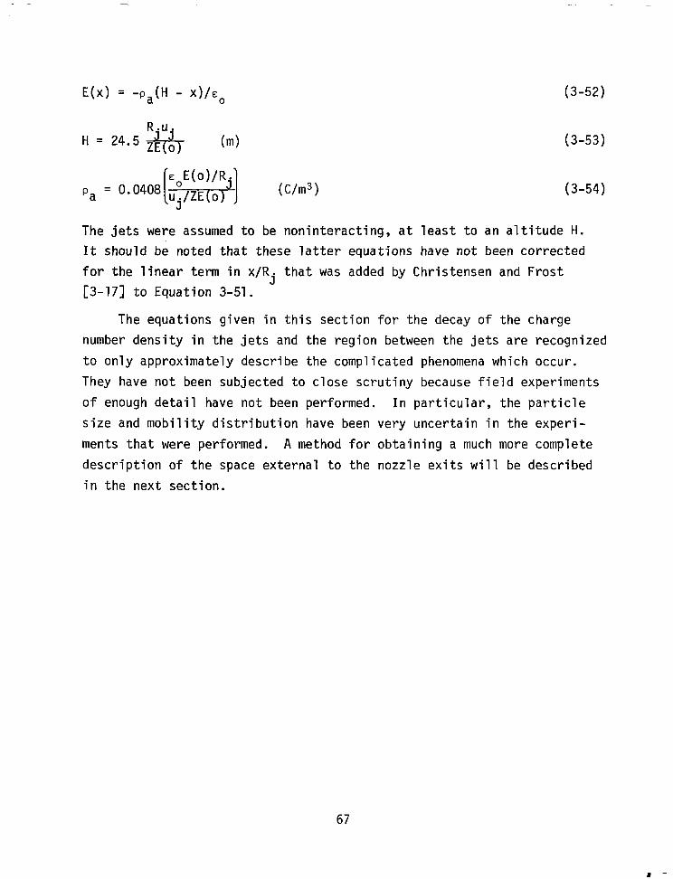
E(x) = -P,(H - xhO (3-52)
R.u. H= 24.5 z; o
73 (4
pa = 0.0408[$$$$-] (C/m3)
(3-53)
(3-54)
The jets were assumed to be noninteracting, at least to an alti-tude H.
It should be noted that these latter equations have not been corrected
for the linear term in x/Rj that was added by Christensen and Frost
[3-171 to Equation 3-51.
The equations given in this section for the decay of the charge
number density in the jets and the region between the jets are recognized
to only approximately describe the complicated phenomena which occur.
They have not been subjected to close scrutiny because field experiments
of enough detail have not been performed. In particular, the particle
size and mobility distribution have been very uncertain in the experi-
ments that were performed. A method for obtaining a much more complete
description of the space external to the nozzle exits will be described
in the next section.
67

References
3-l.
3-2.
3-3.
3-4.
3-5.
3-6.
3-7.
3-8.
3-9.
3-10.
3-11.
3-12.
3-13.
Gourdine, M. C., T. K. Chiang, G. B. Carvin, and A. Brown. "EGD Fog Dispersa ? System Scaling Laws," Paper presented at the AMS's Fourth National Conference on Weather Modification, Fort Lauderdale, Florida, November 1974.
Gourdine, M. C., T. K. Chiang, and A. Brown. "A Critical Analysis of the EGD Fog Dispersal Technique," The Cornell Engineer, pp. 14-35, November 1975.
Ruhnke, L. H. "Warm Fog Modification by Seeding with Unipolar Ions," AMS's Second National Conference on Weather Modification, Santa Barbara, California, pp. 385-388, 1970.
Whitby, K. T. "Generator for Producing High Concentrations of Small Ions," Rev. Sci. Instrum., Vol. 32, pp. 1351-1355, 1961.
Whitby, K. T., R. C. Jordan, C. M. Peterson, and L. W. Rees. "Charging and Decay of Monodispersed Aerosols in the Presence of a Unipolar Ion Source," Final report for USPHS, Grant No. AP00136-02, September 1963.
Whitby, K. T., B. Y. H. Liu, and C. M. Peterson. "Charging and Decay of Monodispersed Aerosols in the Presence of Unipolar Ion Sources," Journal of Colloid Science, Vol. 20, pp. 585-601, 1965.
Chiang, T. K. "Field Evaluation of an Electrogasdynamic Fog Dispersal Concept," Part I, Report No. FAA-RD-73-33, February 1973.
White, H. J. "Particle Charging in Electrostatic Precipitation," AIEE Transactions, Vol. 70, pp. 1186-1191, 1951.
Oglesby, S., Jr., and G. B. Nichols. Electrostatic Precipitation. New York: Marcel Dekker, Inc., 1978.
Lapple, C. E. "Electrostatic Phenomena with Particulates," Advances in Chemical Engineering. New York: Academic Press, 1970.
Arendt, P., and H. Kallman. "The Mechanism of the Electrification of Small Particles in Clouds," Z. Physik, Vol. 35, pp. 421-441, 1926.
Harsha, P. T. "Free Turbulent Mixing: A Critical Evaluation of Theory and Experiment," AEDC TR-71-36, 1971.
Whitby, K. T. "Analysis of Electrogasdynamic Fog Dispersal," Final report to ERDA Contract E(ll-l)-1248, December 1976.
68

3-14; Crawford, M. Air Pollution Control Theory. New York: McGraw- Hill, 1976.
3-15. Cobine, J. D. Gaseous Conductors. New York: Dover Publications, 1958.
3-16. Schlichting, H. Boundary-Layer Theory, 6th edition. New York: McGraw-Hill, 1968.
3-17. Christensen, L. S., and W. Frost. "Fog Dispersion," NASA CR 3255, March 1980.
69
4.0 FOG/JET FLUID DYNAMICS
Figure 4.1 illustrates schematically a number of physical effects
which must be considered in attempting to analyze and plan an experi-
mental field program to test warm fog dispersal by charged particle
techniques. The figure illustrates a jet containing charged droplets as
well as some ions which are propelled by the jet momentum into the
atmosphere. Controversy exists as to whether the droplets reach maximum
height simply through momentum imparted by the jet or through turbulent
diffusion. Turbulence will be induced not only by the jet itself, but
also by neighboring jets as well as the natural turbulence in the atmo-
sphere. It is also unknown as to whether the jet contains only charged
droplets or positive and negative ions as well. In general, it is
assumed that the charged droplets are unipolar charged droplets with a
common polarity. In turn, the size distribution of the charged droplets
leaving the nozzle is not well known.
As illustrated schematically in the figure, the charged droplets
can transfer charge to fog droplets by polarization charging and/or
attachment charging, i.e., diffusion charging and electric field
charging. Also, the induced electric fields may enhance coalescence
with subsequent precipitation of the fog droplets.
Additionally, the interaction of the jet with the atmospheric
boundary layer is not fully understood. In Reference [4-l] some simple
jet analysis without concern for the incorporation of charged particles
were investigated to see the effect of crosswind on the jet. These
models, however, do not provide any insight into how far downstream the
charged particles are carried before they effectively cause precipitation
of the fog droplets. This is a very important problem relative to
nozzle spacing and position with respect to the runway.
In this section, a set of equations is developed which can be
utilized to investigate the behavior of the charged jet interaction with
the atmospheric boundary layer. The equations are developed for
70

-
r-7 ATTACHMENT' / "
0 CHARGING 0
@\ //
/ ooo
I 0 a/
t
CHARGED DROPLETS DROPLETS
0” I r+------ Ioris 0 0
0
oo~~“o 1-A .o 0 0
X
0
0 0
Figure 4.1 Schematic illustration of physical effects involved in warm fog dispersal by a charged droplet jet.

two-dimensional flow. In this case, the jets would be treated as a
plane jet perpendicular to a crosswind. Such arrangement would be
similar to a line of fog dispersal units perpendicular to the crosswind.
The development of the equations is drawn heavily from [4-2, 4-31.
The former references deal with numerical modeling of the atmospheric
boundary layer incorporating turbulence kinetic energy and turbulence
length scale transport equations. The latter reference deals with the
numerical study of cloud electrification in an axisymmetric, time-
dependent cloud model. The equations presented in the aforementioned
references are modified to apply to the case of a plane jet discharging
from the ground into a logarithmic atmospheric boundary layer wind
profile.
In Section 4.1 the standard conservation equations for mass and
momentum are described. In Section 4.2 the equations necessary to
incorporate the effect of transport of water substances are presented
and discussed. The thermodynamic equations are stated in Section 4.3.
In Section 4.4 the equations governing the transfer of charge are
presented. Models currently used in cloud physics programs for
incorporating the effect of polarization charging and/or attachment
charging are also described in this section. Solutions to the equations
are not given nor are the full complement of boundary conditions
developed.
4.1 Momentum Equation
Figure 4.2 lists the momentum equations along with the equation for
conservation of mass. Electric force terms are included to model the
electrical effects on the air motion. The definition of terms is given in the Nomenclature. Little discussion of these equations is necessary
since they are simply the Navier-Stokes equations with the additional
electric force terms added. The standard Boussinesq approximation is made and referenced to an environment state having a constant reference
pressure, p,, and a vertical varying density, <p>. Variables in angle
72

Primitive Variables
'T & = -cp<e>(l + 0.61 q,)$+ <p>Ex + Fx
!h = -c Dt P
<e>(l + 0 61 . q 0.61 q' - L - 'If - ~2 V C P I
+ PT -E, + F, <P’
IT = (P/P,) R/Cp
;
< > designates reference state.
Vorticity and Streamline Variables
a<p>u llJ=r-
a<p>w ax
DU -= Dt
-uw a2<p> + az2
aq; + 0.61 ax
v21JJ = <p>w
where
~=1.2!. P az
and 1 w WC _-- P ax
2~ a<p> - - + <p>g L
1 ae’ - - <p> az a> ax
ak -$ +---
1 aPTEz
ax aPTEx + D
az w
(1)
(2)
(3)
(4)
(5)
(6)
(7)
where
Dw is the vorticity source term.
Figure 4.2 Conservation of momentum equations.
73

brackets represent those of the environmental reference state, and the
primed variables represent the deviation.
Equations 5, 6, and 7 of Figure 4.2 express the equations in terms
of the vorticity and streamline variables. It is believed this formu-
lation of the governing equations will be more convenient and will have
certain advantages relative to numerical solution.
4.2 Conservation Equations for Water Substances
4.2.1 Governing Equations
Figure 4.3 lists the equations governing the transport of water
substances. In this set of equations, the relative velocities, Vc, Vf,
and V , represent the velocity of the average size charged droplet, fog
droplEt, and precipitating droplets, respectively. The effect of both
electrical and gravitational forces on these velocities are taken into
account as described later. The term Pfp represents the rate of auto-
conversion of fog droplets to precipitation droplets, the terms PfA and
P PA
represent the rate of accretion of charged droplets to fog droplets
and of charged droplets and fog droplets to precipitation droplets,
respectively. Finally, the terms PfE and P PE
represent the rate of
evaporation of fog drops and the rate of evaporation of precipitation
drops, respectively. The water substance variables, q, R1, R2, are
simply convenient choices of combinations of water content terms. The
symbol q represents the sum of the water vapor plus the liquid water
content due to charged droplets in the given control volume (pounds per
unit mass of air). The quantity Rl represents q plus the liquid water
content of the fog droplets, and the symbol R2 represents the combined
or total water content of the atmosphere.
The terms on the left-hand side of Equations 1, 3 and 5 represent
the total rate of change of the respective water content quantities.
The first term on the right-hand side of the equality sign, in these
same equations, represents the turbulent diffusion of the water sub-
stances. The terms appearing in the equations which contain the relative
velocities of the various droplets, i.e., Vc, Vf, and V , represent the
liquid water transport due to the motion of the particl!& with respect
74

r
E&&. <P'
KV<p>q - & v l <pxcvc - P PA - 'fA + 'fE + 'pE
9 = qv + Rc
D% PC Dt 1,
<P' l KV<p>RI - + [v l <p>RcVc + v l <P>RfVf]
- 'fp - 'PA + 'pE
R, = qv + Rc + Rf
DE2 1 Dt = yp7 v l tq V<p>R,
+v. <P>llpVpl
‘2 = 9, + R, + Rf + R P
(1)
(2)
+ cv l <P’RcVc + v l <p>RfVf
(5
(3)
(4)
'1
(6)
pfp - rate of autoconversion of fog droplets to precipitation droplets
'fA - rate of accretion of charged droplets to fog droplets
'fE W rate of evaporation of fog droplets
P PA y
rate of accretion of charged and fog droplets to precipitation droplets
P PE
- rate of evaporation of precipitation droplets
Figure 4.3 Conservation equations for water substances.
75

to the air flow. That is, these terms express the fact that the droplets
due to gravitational or electric forces will be moving faster or slower
than the surrounding air and will consequently precipitate or move out
of the control volume.
4.2.2 Mathematical Expressions for Sources and Sinks of Water Substances
To solve the governing equation given in Section 4.2.1, mathematical
models of the source and sink terms for the water substances are
required. Expressions for these quantities are given in Figure 4.4.
The expression for the autoconversion of fog droplets to precipitation
droplets is modified from Chiu [4-31. In this expression, Nf, is the
number of droplets per unit volume, <p> is the reference density of the
air, Do is the relative dispersion of the droplet distribution, and will
need to be determined from empirical results. The term R, is a threshold
value of fog water content for conversion.
2 x lo-3
A value of R. equal to
grams/gram is recommended for the threshold value of cloud
water content in [4-31. A similar value is expected to apply for fog.
The accretion term, Equation 2 in Figure 4.4, represents the mass
growth rate of fog droplets due to capture of the charged droplets. A
similar expression exists for the growth of the precipitation droplets.
The mass growth of the droplets occurs due to the charged droplets moving
with velocity Vc through the fog droplets which are either stationary or
moving with a small terminal velocity, Vf. In general, the relative
velocity of the fog droplets will be small, whereas the charged droplets
particularly near the nozzles will be very high and will become smaller
as they reach higher altitudes in the atmosphere. Similarly, the
precipitation droplets falling through the relatively stationary fog
will accrete fog droplets and carry them to the ground. Also, they will
intercept charged droplets and possibly carry them downward.
In the expression given by Equation 2 in Figure 4.4, n represents
the collision efficiency which is defined as the probability that a
charged droplet will collide with a droplet in its path. The growth of
fog droplets by collision and coalescence with charged droplets as well
as precipitation droplets depends not only on n but also on (1 - <S>),
76

pfp = <P>(llf - fio12 .
1.2 x 1o-4 + 1.596 x lo-l2 Nf/Dop(Rf - Ro) ' Rf - R. > 0
'fA = Nf m$/Vc - Vf IPql - <S>)/<p>
Nf4Trf(l - s)(l + 0.22 Re"2)
'fE = <p'(L2/kTRvT2 + l/<p>qvsDv)
Similar expressions for P PA
and P PE
can be developed.
0)
(2)
(3)
Figure 4.4 Mathematical expressions for sources and sinks of water substances.
77

where <S> is defined as the mean separation probability. This expression
is described in detail in [4-31. The expression (1 - ~9) signifies the
fraction of colliding droplets that coalesce, i.e., the coalescence
efficiency.
Finally, Equation 3 in Figure 4.4 represents the evaporation of the
fog and precipitation drops. The charged droplets will also evaporate,
but because of their small size this is negligible. In the evaporation
expression, L is the latent heat of evaporation, Rv the specific gas
constant for water vapor, Dv the diffusivity of water vapor in air, k
the thermal conductivity of the air, T the temperature of the air, and s
the saturation ratio defined as the ratio of water vapor mixing ratio,
%, to the saturation vapor mixing ratio, q,,.
4.2.3 Water Substance Parameters
The solution of the expressions for sources and sinks of water
describes the governing equations for these parameters. The various
parameter equations shown in Figure 4.5 are explained for fog droplets
only; however, similar expressions can be developed for the charged
droplets and precipitation droplets, respectively. If the fog liquid
water content, Rf, is known at a point in spece, one can consider that
there exists Nf fog droplets per unit volume of air, with mean radius rf.
The number of fog droplets per unit volume, Nf, and droplet radius, rf,
are related to the liquid water content, Rf, as shown by Equation 1,
Figure 4.5. It is necessary to know the distribution function for fog
droplet sizes, nf(r,af) which appears under the integral in Equation 1,
Figure 4.5. This requires further research, but as an example a typical
size distribution for raindrops is the Marshall-Palmer distributions;
N = N,e -ir
with i being a function of liquid water content, Rf:
i = (T~~N~/<P>R)“~
78
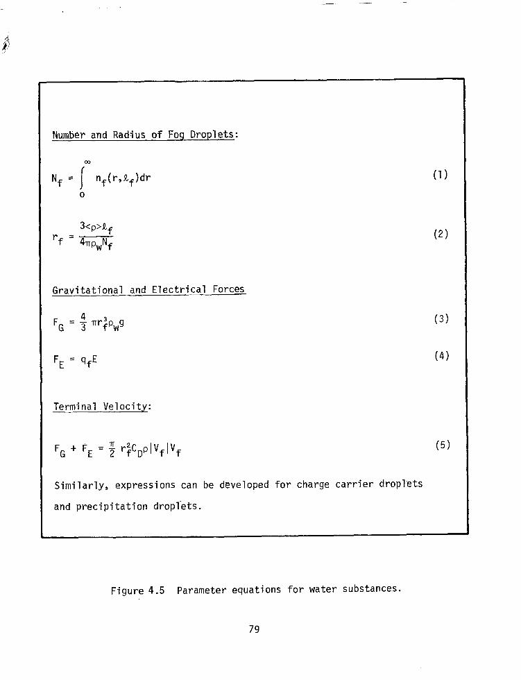
-
Number and Radius of Fog Droplets:
co
Nf = I
nf(r,Rf)dr ('1
0
3<p>llf rf =
4TP,Nf (2)
Gravitational and Electrical Forces
FE = qfE
Terminal Velocity:
FG + FE = $ r;CDp[Vf
Similarly, expressio
(3)
(4)
s can be developed for charge carrier droplets
‘1
and precipitation dropl'ets.
Figure 4.5 Parameter equations for water substances.
79

,
In the Marshall-Palmer distribution, No is given empirically as
0.08 k4, r is the radius of the raindrops, p, is the density of water,
and <p> is the density of air as defined previously. The mean radius of
the fog droplets can then be determined from Equation 2, Figure 4.5.
Knowing the average radius of the fog droplets, the gravitational
force, FG, and the electrical force, FE, exerted on a droplet may be
expressed as shown in Equations 3 and 4 of Figure 4.5. qf is the charge
on a droplet of average size. For this study it can be assumed that:
qf = Qf/Nf
where Q, is the charge density on the total fog liquid water content.
The equations governing charge transport and an expression for calcu-
lating Q, is given in a following section.
Finally, the relative velocities of the fog droplets, Vf, can be
computed from the drag law where the total force acting on the particle
is the sum of the gravitational and electrical forces, Equation 5,
Figure 4.5.
The technique described above can also be used to calculate the
relative velocities of the average size charged droplets and precipita-
tion droplets, respectively. The number concentration of the charged
droplets, however, will depend upon the characteristics of the nozzle.
Solution of the proposed system of equations can be used to carry out
parametric studies of the best droplet distribution for nozzles. Thus
the computational model proposed will allow either (1) determination of
the effect of a nozzle of known droplet distribution, or (2) parametric
study of droplet distribution to provide design criteria for optimum
nozzle performance. The number of droplets is shown in [4-31 to be an
important parameter influencing cloud electrification and is expected
to be a significant parameter in the fog electrification.
80
---.- ---- ..-....... ._....... .-.--._ ._. .__. ..-. ..- ..-.... ---.-.----..-__-.- __..._.

lr-
4.3 Thermodynamic Equations
The form of the thermodynamic equations used by Chiu [4.3] follows
the work of Orville [4.4] and Wisner, et al. [4.5]. The thermodynamic
equation is expressed in terms of the entropy variable, @', as shown in
.Figure 4.6. The form of the entropy variable for saturated and
unsaturated air are given by Equations 2 and 3 of Figure 4.6, respec-
tively. Again, the left-hand term of the equation represents the total
rate of change of the entropy, I$'. The first term on the right-hand
side of the equality sign represents the turbulent diffusion of entropy.
The latter terms of the equation represent the thermal energy change
due to water mass being advected into a fluid medium and reaching thermal
equilibrium with its surroundings.
The saturation mixing ratio, qvs, can be calculated from Equation 4,
Figure 4.6, where the equilibrium vapor pressure over water, es, is
given by Equation 5. The temperature, T, is directly related to the
potential temperature, 8', through the definition of potential tempera-
ture given by Equation 6;Figure 4.6.
4.4 Equations Governing Electrical Properties
4.4.1 Governing Equations
Figure 4.7 lists the various equations which can be used to simulate
the electrical properties of the fog and jet interaction. The total
space charge density, pT, is given by Equation 1 of Figure 4.7. It is
observed that pT appears in the Navier-Stokes equations relative to the
electric force field. This is one of the most important parameters
which has not been modeled correctly in previous analyses. If the
precipitation process takes place by electrical forces acting on the
charged fog droplets, then the development of this space charge and its
distribution at steady state is essentially the controlling parameter to
assure effective fog dispersal.
In Equation 1, Figure 4.7, the effects of large ions are ignored
which assumes that the growth and decay of the fog is not simulated in
a contaminated atmosphere where most large ions form. This assumption
must be examined for an airport in an urban environment. 81
. ;;T + af(; + Gf) l ;T
+ Ep(; + cp) l ;;T]
0' = 0'/0 + Lqv/CpTa
@' = e'/e + Lqvs(e')/CpT,
q VS
= 0.622 e,/(p - es)
‘(T e S
= exp[19.07 T - 4782.9/
T = <e>(P/Po)R'cp
(unsaturated)
(saturated)
(‘1
(2)
(3)
(4)
35.9)] (5)
(6)
Figure 4.6 Thermodynamic equations.
82
I
--- ----- -._. --.. ._... - --_-- - _.

-
PT = e(nl - n2) + 9, + Q, + Q,
E = -VI$,
V20e = -P&
0)
(2)
(3)
Dnl,2 - Dt -v(?nl,2Zl,2E - Km,,2) + G - anln2
_ [E&z], - [E&?-], - gq,
OQc _ - - -v(QcVc - Dt KVQ,) + e[(sn,/stIc - bn2/Wcl - (6Qc/‘t)coal
f
- (6Qc/fX)coal - (6Qc/~t)polf - bQc~~t)pol (5) P P
DQf - = -v(Q,V, - Dt KVQ~) + e[(6n,/6tIf - @n,/W,l + bQ,/W coalf
- (6Qc/6t)coal + bQc/dpolf - (6Qf/6t)pol (6) P P
-v(Q,V, - KOqp) + eC(snl/6t)p - (6n2/6tIpl + (~Qc/6t)coal P
+ (6Qf/6t)coal + bQc/6t)pol + bQf/6t)pol (7) P P P
Figure 4.7 Equations governing electrical properties.

The electric field strength can be related to an electric potential,
Ge (see Equation 2, Figure 4.7). The relationship between the electri-
cal potential and the space charged density is then given by Equation 3,
Figure 4.7.
Equations 4, 5, 6, and 7 represent the conservation of ion and
charge density. n1,n2 represent the positive and negative free small
ions, while Q,, Q,, and Q, represent the space charge densities associ-
ated with the charged droplets, the fog droplets, and the precipitating
droplets, respectively. Again, the left-hand terms of the five equations
represent the total rate of change of the quantities indicated. Note
that Equation 4 represents two equations-- one for negative ions and one
for positive ions. The subscript (1,2) is simply a concise notation.
One observes from Equation 4, Figure 4.7, that the current
densities for the macroscopic transport of ions is made up of contribu-
tions from electrical conduction, 'nl 2Zl 2e, and turbulent diffusion
- KVnl,2. Besides the transport term:, i&s can be formed or generated
by cosmic ray ionization at various heights. This is unlikely to be
important in the fog problem but is represented by the term G in the
equation. The rate of ion loss is mainly controlled by ion attachment
to the droplets in the flow field (6nl 2/6t)c, (6nl 2/8t)f and
(6nl,2/Wpg and by ionic recombinatio; between ion: of opposite
polarity, -onln2. The effect of charge on droplets being released as
free ions during evaporation of the water droplets is also included in
the last three terms of the equation as described later.
In Equations 5, 6, and 7, Figure 4.7, the charge densities associ-
ated with all three forms of droplets are transported both by their
relative velocities with respect to the air motion and by turbulent
diffusion, V l (QV, - KVQ,). The second term in each of these equations
represents electric charging of the droplets through ion attachment,
e[(6nl/Wc - b2/Wcl. Finally, the droplets can also be electrified
and charged due to the polarization charging mechanisms when particles
collide with each other and then separate in electric field (6Q/6t)pol
and through charge transfer when charged droplets collide and coalesce
with fog droplets and precipitating droplets, (6Q/bt)coal. The charge
84

density related to, say, 'the charged droplets' is considered to be
partially transferred to the charge density associated with, say, 'the
fog droplets' according to the number of charged droplets coalescing with
fog droplets.
4.4.2 Ion Attachment to Droplets --------
Figure 4.8 lists the equations governing ion attachment to the
various droplets. These equations assume that ion attachment occurs by
ionic diffusion and electrical attraction only. A physical discussion
of droplet charging by these mechanisms is given in Section 3.0. In
this section the models are static models where the effect of relative
velocity of the droplets with respect to the field and air flow is
neglected. The equations given in Figure 4.8, however, take into
account the effect of droplet motion at least in an approximate manner.
On the other hand, these equations neglect the effects of ambient space
charge around the droplets and effects due to physical or chemical
properties of the droplet surfaces.
Equation 1 of Figure 4.8 illustrates that the total rate of attach-
ment of ions is expressed in terms of a simple superpositioning of the
rate of attachment of ions due to diffusion and the rate of attachment
of ions due to electric field effects. The two expressions for the rate
of ion attachment are based on the assumption that each works separately.
In actual fact, the two attraction processes will operate simultaneously,
however, there is no rigorous analytical solution presently available in
the literature to compute this effect. Therefore the assumption of
superpositioning is made. Evidence given in the literature suggests
that the method of superpositioning will not lead to errors greater than
15%. The equations in Figure 4.8 are developed for fog droplets,
however, similar expressions pertain to the charged and precipitation
droplets.
The expression for the ionic diffusion is given by Equation 2,
Figure 4.8. One observes from this equation that when the relative
velocity of the fog droplets is zero, the equation reduces to the simple
static diffusion attachment described earlier in Section 3.0.
85
rota1 Rate of Attachment of Ions (i.e., due to ionic diffusion and electrical (field) attachment)
1 1 6nl,2 tit f = NfC(&,2)D + (&,2)El
Ionic Diffusion
(I’,& = 4nrfDl,2n1,2[1 + (rfVf/2~Dl,2)"21
tlectrical Attraction
1. 9f ' 9,; (i')E = 0, && = n2Z2hf/Eo)
2. qf < 9,; (?'), = -nlZl qf/Eo3 ($4 = o
3. 9, ' qf ' -qs
Case 1: E same direction as Vf
(?')E = O; 9, ' qf ' 0; IVfl ’ Z’IEI (il)E = -nlZlhf/Eo); 0 ’ qf ’ -9,; lvfi ’ $jEi (‘dE = nlZl IEihrf)[l - (sf/qs)12; lVfi < zl IEi (‘dE = n2Z21Ei(3$)[1 + (qf/qs)12
Case 2: E opposite direction of Vf
(‘& = n2Z2hf/Eo); q, ' qf ' 0; IV,/ ' Z21E1
(-i2)E = 0; 0 > qf > -q,; lVfi ' Z21E1
tidE = n2Z2iE1(3$)[1 + (sf/qs)12; Pfl < $IEl
til JE = nlzl i Ei hr;)Cl - hf/q&12
(‘1
(2)
(3)
(4)
(5)
(5i)
(5ii)
(5iii)
(5iv)
(5v)
(5vi)
(5vii)
(5viii)
Figure 4.8 Ion attachment.
86
The mathematical expression for the electrical field attachment of
ions is somewhat more cumbersome than that for diffusion attachment.
Ion attachment due to electric field attraction to a droplet of radius,
rf' in an electric field, E, can be written in three, different forms,
depending on the polarity and magnitude of the net charge, qf, of the
droplet. Equation 3 represents the case where the droplet charge is
positive and greater than the saturation charge. In this case no
positive ions attach. Equation 4 gives a similar result for when the
droplet charge is negative and exceeds the magnitude of the saturation
charge.
Equation 5, shown in the figure, expresses the fact that for
q, ' qf ' -qp the direction of the electric field relative to the
direction of veloc.ity of the droplet is significant. Equation 5, Case
1, illustrates the mathematical form of the expression for the ion
attachment rate where the field is in the same direction as the direc-
tion of the velocity of the droplet. In this case the rate of attach-
ment of positive ions also depends upon the magnitude of the relative
velocity of the droplet to the drift velocity of the droplet, defined as
the mobility, Zl 2, times the magnitude of the electric field [El. For
Case 2 where the'electric field is in the opposite direction of the
relative velocity of the droplet, the situation is reversed and the
rate of attachment of negative ions is dependent upon the magnitude of
the relative velocity to the drift velocity.
The expressions for electrical field attachment given in Figure 4.8
are based on the assumption that the electric field is parallel to the
direction of droplet motion. No analytical solution is available for
the case where the electric field is not parallel to the velocity of the
droplet. However, for the simplest method of solution, it is assumed
that meaningful results can be obtained by replacing IEI by the com-
ponents of IEl along the direction of relative velocity.
A physical explanation of the equations in Figure 4.8 may be gained
by inspection of Figure 4.9. When a droplet is totally positively or
totally negatively charged, the ion fluxes to the droplet have similar
mathematical forms. The rate of ion attachment depends only on the net
charge of the droplet and has nothing to do with the ambient electric
fields nor the terminal velocity of the droplet. If the droplet is 87

t P Z,E I I I \ \ \
.
Q ZzE carv
9f = 0
(a>
1 E
I d Z2E + - ZIE P- I
J3 rf(l +
b) Figure 4.9 Ion capture cross sections of a droplet.

polarized in the electric field and at rest with respect to the ambient
air, only positive ions can be attracted directly to the negatively charged
region of the droplet, while the negative ions on the same side of the
droplet can never become attached to the drop but are driven away by the
electric forces. Conversely, on the other side of the droplet, only
negative ions can reach the droplet at its positively charged region.
This situation changes when the droplet has a relative velocity
with respect to its environment. To illustrate these changes, consider
Figure 4.10(a). Here the relative velocity of the droplet is greater
than its drift velocity. In this case, focusing attention on the lower
left-hand corner of the figure, the velocity imparted to the droplet due
to drag of the air is greater than its drift velocity. Therefore, it is
carried towards the positive charged region of the droplet, whereas if
it were at rest it would be repelled. Since it cannot attach to the
positively charged region, it is swept around the particle and can
either pass by the droplet if the droplet is completely positively
charged or can be attached to the negative region behind the droplet if
the droplet has some negative charge.
The negatively charged droplets illustrated in the right lower
corner of Figure 4.10(a) will have both the relative velocity and drift
velocity directed towards the droplet and therefore will attach on the
front portion of the droplet. In turn, the two ions illustrated at the
top of Figure 4.10(a) will both move away from the droplet. The
positive ion moves away because the droplet's relative velocity is
greater than the drift velocity caused by the electric field. Therefore
the positive ion can never catch up to the droplet. The negative ion
moves away even if the relative velocity of the particle were zero,
because the negative region of the droplet repels the ion. This situa-
tion is clearly contained in Equations 5i and 5ii, Figure 4.8.
Inspection of Figure 4.10(b) illustrates the case where the
relative velocity of the droplet is less than the drift velocity of the
ions. This case is exactly identical to the case of zero droplet
velocity. However, the negative ions will attach at a faster rate
because their velocity relative to the droplet is increased by the
89

vf I
I I
(a>
+ vf ZIE P
I I I I I
0 +
b)
Z.2E
Q vf
\ \ I I I I vf Z2E
Q
I "f
Figure A:10 Schematic of ion attachment by electrical field effects with moving droplets.

p
drift velocity, whereas the positive ions will collect at a slower rate
because their velocity relative to the droplet is decreased due to the
drift velocity. This effect is contained in Equation 5iii, Figure 4.8.
Similar explanation of Equation 5, Case 2, can be given.
4.4.3 Release of Free Ions Due to Evaporation
To account for the increase in free ions in the terms 6nl 2/6t due
to evaporation of the droplets,the following rule is proposed iy Chiu
[4-31. In his cloud electrification model, he allows part of the net
charge associated with cloud water to be released as free ions as the
cloud water content decreased because of evaporation. He assumes the
amount of net charge released to occur in such a way that the net charge
per unit area of droplet surface remains constant during the shrinking
of the droplet due to evaporation. Although this is a gross assumption,
it at least prevents the charge carried by droplets from becoming too
large to be realistic when the droplet shrinks during evaporation.
4.4.4 Polarization Charging Mechanism
An expression for the term (6Q/6t)pol occurring in the charge
transport equations must be developed. The simplest case of charge
redistribution due to polarization occurs between two spherical droplets
when they contact each other and then separate in an electric field.
Consider a large drop of radius, rf, with net charge, qf, which collides
with a small droplet of radius, r , with net charge, q , under the
influence of an electric field. ifter the contact, chirge will be
redistributed between the two droplets so that the net charge of the
large droplet becomes qf, while that of a small droplet becomes qc.
Figure 4.11 shows the mathematical relationships. The term, Aq, is the
charge transfer between the droplets. The terms A and B in Equation 2,
Figure 4.11, are positive nondimensional coefficients which can be
written in terms of the ratio between the radii of droplets as shown in
Equation 3. The positive nondimensional constants, y, and y2,depend
only on the ratio between the radii of the droplets. Latham and Mason
[4-61 show for the particular case where rc << rf, yl = 7r2/2 and q = .rr2/6. Inspection of the equation for Aq shows that the amount of
91

Upon collision but not coalescence of a charge carrier and fog
droplet under the influence of an electric field
q; = qf - Aq;
where
q; = qc + Aq (1)
Aq = 4~eo-y,IElcos(E,rfc)r~ + Aqf - Bqc (2)
A= Y2(rc/rf)2 .
1 + Y,(rc/rf)* ' B= 1
1 + Y,(rc/rf)2 (3)
Figure 4.11 Charge redistribution during polarization charging.
charge transferred between a pair of droplets under an electric field E
depends on the original net charge on the particles, (qc,qf), the sizes
of the particles, (rC,rf), the strength of the local electric field, /El,
and the angle between the electric field vector, E, and the position
vector of the small colliding droplet with respect to the center of the
large droplet, ref. The cosine of the angle between E and rcf is
denoted with cos(E,rcf). After some algebra, Chiu [4-31 shows that
the rate of change of the charge density of the fog liquid water with
respect to time is given by the expression shown in Figure 4.12. Where
c.9, the mean separation probability and <cos a,>, the mean value of
cos ~1~ for all colliding droplets, are given by Equations 2 and 3 of
Figure 4.12, respectively. The angle ~1~ is a measure of the relative
location of the colliding droplet with respect to the impacted droplet.
Equation 1 of Figure 4.12 shows that the charging rate of a droplet
depends directly on the size of the droplet, rf, the collision effi-
ciency, n, the separation probability of the colliding drops, <S>, the
92

"qf -= 6-t ~fl~cflNc(nr~){4r~oullEl cos (E,Vcf)rE <cos al> - Aqf + BqckS>
(1
r/2 <s> =
i S(al)ilTrF sin al cos crl dal/rrr; (2
0
T/2
<cos al> = i
~S(CX~) sin al cos 2 al dc+S> (3 0
Rate of Polarization Charging .--II_-----
bQc/~t)polf = Nfbqf/"t) (4
Rate of Coalescence Charging .--~-
("Qc'6t)coalf = Nfhf IVfclNp$(l - -+)qc3 (5
Figure 4.12 Polarization and coalescence charging mechanism.
number concentration of the colliding droplets, NC, and the speed of the
small droplets relative to the large droplet, IVcfl. The equation
indicates that the more droplets which collide with the large droplet
and then separate from it per unit time, the faster the large droplet
can be charged. For each collision and separation, more charge is
separated between droplets. It is apparent that the local electric
field increases if (1) the ambient electric field tends to be parallel
to Vcf, (2) the size of the droplets increases, and (3) the value of
<cos al> increases. The charging rate, of course, is also affected by
the charge already accumulated on the interacting droplets, i.e., qf
and q,. The final expression for the term (6Q/6t)pol is then given by
Equation 4, Figure 4.12. This expression assumes that the fog droplets 93

are separated far enough from one another in the fog that the 8qf/8t
expression in Figure 4.12 can be applied to all of the fog droplets in a
unit volume of air.
The above discussion of the polarization charging mechanism is, of
necessity, brief and the reader is referred to the more complete deriva-
tion given by Chiu [4-31.
4.4.5 Charge Transfer During Coalescence
From Equation 1, Figure 4.12, it is apparent that only <S> fraction
of the colliding droplets separate from the larger droplet to make the
polarization charging mechanism work. There is, therefore, (1 - <S>)
fraction of the colliding droplets which coalesce with the larger drop-
let. In such conditions, it is assumed that the net charge on the
droplet transfer to the larger droplet. If q, is the average charge on
the charged droplets before collision and coalescence, then the form of
(~Qc/~t)coal in Equations 5, 6, and 7 of Figure 4.7 can be expressed as
shown by Equation 5, Figure 4.12.
4.5 Utility of Equations
The preceding equations represent a set of governing equations
which, if solved simultaneously by numerical techniques, will provide,
at least, qualitative solution to the rate at which fog droplets can be
precipitated by electric charged particles sprayed into the atmosphere.
Of course, many assumptions in the model are involved and must be
examined once solutions are available and experiments are carried out.
A number of the parameters which are needed as input to the various
semiempirical expressions appearing in the governing equations are not
well known. However, the model can be applied to parametric studies and
the sensitivity of the fog dispersal technique to the various parameters
can be established.
In addition to the unknown empirical parameters, a complete set of
initial conditions and boundary conditions must be established before
the solution of the system of equations can be achieved. Work in this
area is continuing and will be reported at a later date. 94

References
4-l.
4-2.
4-3.
4-4.
4-5.
4-6.
Christensen, Larry S., and Walter Frost. J'Fog Dispersion," NASA Contractor Report 3255, prepared by FWG Associates, Inc., Tullahoma, Tennessee, under Contract No. NAS8-33095 for Marshall Space Flight Center, Huntsville, Alabama, March 1980.
Becker, Bryan R. "Cooling Tower Recirculation as Influenced by the Local Atmospheric Flow Field, a Numberical Study," PhD Dissertation, The University of Tennessee, December 1979.
Chiu, Chin-Shan. "Numerical Study of Cloud Electrification in an Axisymmetric, Time-Dependent Cloud Model," Journal of Geophysical Research, Vol. 83, No. ClO, Octobem,.
Orville, H. D. "A Numerical Study of the Initiation of Cumulus Clouds over Mountainous Terrain,"- Journal of Atmospheric Science, -- Vol. 22, p. 684, 1965.
Wisner, C., H. D. Orville, and C. Myers. "A Numerical Model of a Hail-Bearing Cloud," Journal of Atmospheric Science, Vol. 29, p. 1160, 1972.
Latham, J., and B. J. Mason. "Electrical Charging of Hail Pellets in a Polarizing Electric Field," Proceedings of the Royal Society of London, Series A, 266, 387, 1962.
95
5.0 FIELD EXPERIMENT
Simultaneous with the analytical modeling of the fog dispersal
technique and the nozzle design study, advanced planning of a field
study to verify the charge particle fog dispersal systems is needed.
This section discusses meteorological measurements which must be consid-
ered (rates and accuracies), site requirements, spatial configurations
of units,and necessary instrumentation, i.e., tower, transmissometer,
electric field mills, cloud particle and nuclei counters, etc.
5.1 General Requirements
Electrostatic fog dispersal, although shown effective in the
laboratory, has not been demonstrated conclusively in the field. It is
essential that to accurately assess charged particle fog dispersal
techniques, a comprehensive field experiment be designed.
The field experiment must determine if there is any improvement in
visibility and the time, duration, location, and degree of improvement.
Any natural fog dissipation, warming, advection of dry air, change in
spectrum of condensation nuclei, etc. must be accounted for and distin-
guishable from the conditions produced by the fog dispersal system.
To examine the charging characteristics of particular charge
particle spray guns the electric field and changes in the electric field
with space and time need to be measured. The charge on the precipitated
drops will determine the charge transfer efficiency between the particu-
lar fog drops and charge carriers.
There are a number of site requirements for a field experiment of
this nature. The aviation industry is the most likely industry to
benefit from fog dispersal; therefore, the site should be at an airport
or approximate the terrain of an airport. Airports are characterized by
flat terrain, low vegetation, and few tall buildings in the runway area.
For convenience, an area where fogs occur regularly and predictably has
obvious advantages. 96

An area that has different types of fog, i.e., advection, seacoast,
and urban fogs under different prevailing weather conditions might
eliminate the need for testing at different sites. The size of the
field experiment can be reduced if the normal mean wind direction during
foggy conditions is known. This allows the field instruments to be
arranged along the mean wind thus making an essentially two-dimensional
experiment which greatly reduces the number of necessary measurement.
Any nearby meteorological recording stations are of obvious value.
One possible geometrical configuration for the proposed field
project is shown in Figure 5.1. This shows a minimum configuration. A
larger test array is required for runs during higher mean wind condi-
tions. The exact size of the array is under investigation. The number
of units required to dissipate fog in crosswind conditions depends on
the wind velocity and time required for visibility to improve. The time
required for visibility to improve to 457 m (1,500 ft) (required visi-
bility for aircraft landing) is estimated at 14 minutes.
For 2.24 m/s (5 mph) crosswind conditions, the wind drifts 1,878 m
(6,160 ft) in 14 minutes. Therefore, to disperse fog with 2.24 m/s
(5 mph) crosswind conditions requires a matrix of units at a 58 m
spacing. This will be more carefully defined from the results of the
on-going studies described in Sections 3.0 and 4.0.
Figure 5.1 illustrates control areas containing an instrumented
tower and transmissometer array located at positions of the test site
upwind and downwind. A similar arrangement of towers and transmis-
someters at the test site will allow for realistic three-dimensional
analysis of the fog life cycle. The influence of a metal tower on the
electrical field is being investigated.
5.2 Required Measurements
The meteorological variables that need to be monitored in order to
verify and analyze the effectiveness of charged particle fog dispersal
are discussed in this subsection. Criteria for a minimum but effective
field project are discussed. A suggested list of rates and accuracies
for the proposed field project are given in Table 5.1. It should be 97

Control Area
a---@
Test Area
0 0 0
0
0
Spatial Configurations -1
El
Control Area
/ / 0 Towers T, q, W
+ Field Mills, E @ Transmissometers, V
lxl Particle Counters, So l Charged Particle Units
El Glass Slides, D
Figure 5.1 Schematic of Site Arrangement for Field Testing.

I -- ;‘\ P 5 i/
Table 5.1 Rates and Accuracies of Meteorological Variables.
T
P
q
V
- 1 W
E _
sO
R
'n
J / 1 I_
I J I
Variable
Temperature
Pressure
Relative humidity
Visibility
i--- _- i Turbulent wind
Electric field -._ __ - -- -- .--- Particle spectrum concentration versus size
Precipitation rate
Condensation nuclei
Locations Accuracy Frequency .--_
Three levels, 0.1" c l/60 Hz three towers
Local airport
Three towers
Three towers, three axes
0.1 mb l/3600 Hz (hourly)
1% l/60 Hz
lm l/60 Hz
Three levels, three towers
0.1 m/s 1 Hz
Three locations 10 v/m l/60 Hz
Three locations 102/m3 l/60 Hz
Three locations 1 drop/ l/900 Hz mm2/min (15 min)
-- One location 102/m3 l/900 Hz upwind
** Optional Measurements ** : = :.= __ ~=; :L__..~= . .
HI Inversion height
Y Lapse rate above tower height
One location
Local airport
Local meteorological station
10 m ---
10 m/s l/3600 Hz
1" C/m Twice daily
** Synoptic Conditions ** =;._.=:..=-:;z.z2mm ;::: ~-~-_ __~-
Hourly synoptic scale weather conditions should be analyzed for fog extent and surrounding conditions. Advection rates of temperature and humidity.
99
noted that these accuracies and frequencies can be attained from commer-
cially available instrumentation and that some leniency may be accepted
while still producing meaningful data. The rates and accuracies listed
for the wind field are for turbulence measurements and need not be that
sensitive at all three locations.
5.2.1 Three-Dimensional Wind Field
The three-dimensional wind field needs to be known at a minimum of
three locations upwind and downwind from the test site and at the test
site. The wind field must be measured to the height of desired fog
clearance. If the terrain at and around the test site is flat and
homogeneous, turbulence measurements are really needed only at one
location, ideally at the test site. The geostrophic wind can be inter-
polated from maps obtained from surrounding National Weather Service
Stations.
5.2.2 Temperature and Humidity Fields
The temperature and humidity fields need to be known at the test
site and at both control areas. To determine the stability of the
atmosphere the temperature lapse rate must be measured. It is convenient
to simply locate a reference thermocouple junction at one level on the
meteorological towers and temperature differential instruments at other
levels. Humidity need only be measured at one level of each tower if
there is sufficient mixing. These measurements are needed to determine
if any warm or dry parcels of air advect into the area.
5.2.3 Visibility
The purpose of fog dispersal is to improve visibility. Therefore,
one of the more important parameters to measure is visibility. Visi-
bility measurements need to be made on three axes: along wind, crosswind,
and in the vertical. It is convenient to mount a transmissometer at the
top of each tower for the vertical measurement. The horizontal measure-
ments can be made by either transmissometers or backscatter lidars. It
100

is important that accurate measurements be made at the site and both
control areas.
5.2.4 Cloud Physics
The types and spectrum of condensation nuclei prior to the onset
of fog will determine the type of fog which occurs although the gasoline
engine exhaust may have some effects which must be considered. Monitoring of the nuclei for changes in number or species should be used as a control
to determine what changes are instrumental in the fog dissipation.
The fog droplet spectrum, being the direct cause of reduced visi-
bility, must be monitored as continuously as possible at the site and at
both control areas prior to, during, and after the field test. The
theory of charged particle fog dispersal is based on changing the number
and or sizes of fog droplets. Therefore, any accurate assessment of the
dispersal technique must include a complete time history of the droplet
spectrums at the control areas as well as at the test site.
Charged particle fog dispersal theory is based on enhanced fog
droplet precipitation; therefore, the precipitation rate needs to be
monitored as continuously as possible at the test site and at the
control areas. The size of the precipitating droplets will aid in
determining the mechanism behind charged particle fog dispersal.
5.2.5 Electric Field
Charged particle fog dispersal enhances the precipitation rate by
enhancing the local electric field. To determine the efficiency with
which the nozzle enhances the electric field, measurements are needed.
The electric field need only be monitored at one surface location in the
control areas; however, at the test site an array of surface mills and
an elevated mill are required for optimum data collection.
5.3 Instrumentation --_------
Tower instrumentation would consist of standard three-dimensional
wind sensors commercially available from a number of manufacturers.
Thermocouple junctions at a number of heights on each tower with an
101

internal electric reference in the recorder will provide the absolute
temperatures and the temperature lapse rates up to the height of the
towers. An aspirated humidity sensor on each tower will provide
continuous monitoring of the relative humidity and aid in interpretation
of the natural onset and breakup of fog.
Visibility measurements can be made by either of two methods:
transmission or backscatter. Transmissometers measure the percent of
light received to that transmitted a chosen distance away. Backscatter
instrumentation measures the percent of light scattered back to the
transmitter. Transmissometers use either a chopped incandescent transmit
signal or a continuous laser transmitter. The incandescent instrumen-
tation utilizes a full-band photo-electric cell receiver while the laser
utilizes a selective small-band photo cell. The laser circuit allows
the beam to be split into the three orthogonal directions by use of
partial reflectors thus requiring only one transmit circuit at each
site. However, the incandescent instrumentation has the advantage of
low cost.
The electric field is measured with electric field mills. Electric
field mills are of many different designs but most field mills are based
on alternately exposing and shielding an electrical plate to the atmo-
sphere. One particular design is illustrated in Figure 5.2 [5-l]. A
rotating disk with slots, exposes and shields a number of metal studs.
The larger slots allow for the direction of the electric field to be
determined. A sample output is shown illustrating the peaks formed by
the larger slots indicated with a "P." A change in intensity is shown
and indicated with a "C." Since large structures significantly alter
the electric field, the meters must be located in a region at least ten
times the height of such structures or trees away. The measurement of
electric fields is not at all a routine measurement. Considerable
research is currently going on to improve field mill technology. The
most current instrumentation should be used.
To measure the electric field at tower height, a field mill could
be mounted at the top of the tower. A graph of the ratio of the resultant
field at the top of a structure, ET, to the inducing field, E, as a
102

Metal Vaned Wheel
Insu with
lating Ring Metal Studs
Earthing * cup
CP P P
--
Oscilloscope Output
.tmeter
Figure 5.2 Electric field mill [5-l].
103

function of structure dimens-ion, H/R, (height divided by the radius) is
shown in Figure 5.3 [5-21.
The cloud droplet spectrum can be measured with gelatin slides or
a backscatter lidar. The gelatin slides are inexpensive, but require
labor-intensive viewing with a microscope; moreover, they did not prove
very successful during the Panama experiments and would require careful
preparation and application to provide meaningful results. The back-
scatter lidar gives a continuous measure of the droplet spectrum but is
expensive. The.condensation nuclei can be measured with standard aiken
counters.
The preceding brief discussion of instrumentation illustrates that
most instrumentation required to verify the charged particle fog dispersal
technique is commercially available. Some of the instrumentation needed
to make measurements of the accuracy desired, however, are relatively
expensive, for example, backscattering lidar. Obviously, cost of the
experiment is an important consideration , and work in developing a meaningful
experimental plan is on going.
The one area where measurement techniques may require development
is electric field measurements. Presently, a program is being carried
out at the Naval Research Laboratories, Washington, D.C., to develop a
new electric field mill. Work carried out at Socorro, New Mexico, has
produced a successful electric mill, but these are not commercially
available and require appreciable amounts of machining when built on an
individual basis [5-33. Evaluation of electric field measurement
techniques is continuing.
References
5-l. Mason, G. J. The Physics of Clouds, 2nd edition. Oxford: Claredon Press, 1971.
5-2. Anderson, R. B. Lightning, Vol. 1. Academic Press, 1977.
5-3. Christian, Hugh, Personal comunication, July 1980.
104

1000
800 -
600 -
400 -
200 -
loo-
80-
60-
40-
20-
I I I I I I I I I 10 20 30 40 50 60 80 100
ET/E -
2
200
Figure 5.3 Influence of tower structure on local electrical field [5-21.
105

6.0 CONCLUSIONS
This study has reviewed the Panama Canal charged particle, fog
dispersal field test program, looked in-depth at the nozzle character-
istics of a charged particle spray nozzle, formulated the basic governing
equations to analyze a charge jet interaction with the fog environment
and outlined some basic requirements of a field program which would
verify the charged particle fog dispersal technique.
The review of the Panama Canal experiment indicates that the results
are inconclusive as to whethera cleared region can be maintained for
a sufficient period of time and as to the values of certain physical
parameters required to modify and improve the design of the fog
dispersal system hardware.
The in-depth study of charged particle nozzle characteristics suggests
that certain modifications to the design of the previous nozzle used
in the Panama Canal experiment may significantly enhance the amount
of charge which can be induced on the charge carriers. Since the time
for maximum charging of particles in a corona region are on the order of
milliseconds, and the droplets pass through the supersonic nozzle used
in previous experiments on the order of microseconds, techniques for
exposing the particle charge carriers to the corona discharge for a
longer period should be developed. Work in this area is proceeding.
The basic equations which govern the jet interaction within a fog
environment once the charged particles have left the nozzle have been
formulated. The system of equations is essentially the same as used in
cloud electrification studies; however, modification of the boundary
conditions is required for solution of the problem.
A study of the instrumentation needed and its availability to carry
out a full, in-depth field study of the fog dispersal technique utilizing
charged particles indicates that much of the instrumentation is com-
mercially available. For several of the measurements such as droplet
size distributions, a tradeoff between cost and accuracy is an important
106

consideration, e.g., the use of backscattering lidar versus gelatin
slide techniques. Measurements of electric field strengths is one area
where commercial instruments are apparently not available. Electric
field mills have been developed by a number of separate research groups.
These mills can be built on an individual unit basis to carry out
the necessary measurements for verification of the charged particle
warm fog dispersal system. Thus extensive development costs of
instrumentation are not anticipated.
107

1. REPORT NO. 2. GOVERNh&T ACCESSION NO. 3. RECIPIENT’S CATALOG NO.
NASA CR-3440 4. TITLE AND SUBTITLE 5. REPTRT O-ATE
June 1981 Charged Particle Concepts for Fog Dispersion
7. AUTHOR(S)
Walter Frost, Frank G. Collins, and David Koepf 9. PERFORMING ORGANIZATION NAME AND ADDRESS
FWG Associates, Inc. R.R. 2, Box 271-A Tullahoma, TN 37388
12. SPONSORING AGENCY NAME AND ADDRESS
6. PERFORMING ORGANIZATION CODE
-~ 8. PERFORMING ORGANIZATION REPOR
10. WORK UNIT, NO.
M-352 11. CONTRACT OR GRANT NO.
NAS8-33541 ,S. TYPE OF REPOR-; 8 PERIOD COVEI
Contractor Report National Aeronautics and Space Administration Washington, D.C. 20546
15. SUPPLEMENTARY NOTES
Marshall Technical Monitor: Dennis W. Camp Final Report
,..I. SPONSORING AGENCY CODE 505 44 19
ICI. ABSTRACT
Charged particle techniques hold promise for dispersing warm fog in the terminal area of commercial airports. This report focuses on features of the charged particle technique which require further study. The basic physical principles of the technique and the major verification experiments carried out in the past are described. The fundamentals of the nozzle operation are given. The nozzle characteristics and the theory of particle charging in the nozzle are discussed, including information from extensive literature on electrostatic precipitation relative to environmental pollu- tion control and a description of some preliminary reported analyses on the jet characteristics and interaction with neighboring jets. The equation governing the transfer of water substances and of electrical charge is given together with a brief description of several semi-empirical, mathematical expressions necessary for the governing equations. The necessary ingredients of a field experiment to verify the system once a prototype is built are described.
-- 17. KEY WORDS 18. DISTRIBUTION STATEMENT
Warm fog Unclassified - Unlimited Fog dispersal Aviation safety Aviation meteorology
Subject Category 47
,S. SECURITY CLASSIF. (of thh repart)
Unclassified
20. SECURITY CLASSIF. (of this PattO) NO. OF PAGES
I
22. PRICE
Unclassified 120 A06
For sale by National Technical Infornmtion Service. Springfield,
NASA-Langley, 1981