Characterizing the Degrading Effects of Scattering by ... · forward scattering (Mie scattering)...

Paper: ASAT-16-140-SP

16th

International Conference on

AEROSPACE SCIENCES & AVIATION TECHNOLOGY,

ASAT - 16 – May 26 - 28, 2015, E-Mail: [email protected]

Military Technical College, Kobry Elkobbah, Cairo, Egypt

Tel : +(202) 24025292 – 24036138, Fax: +(202) 22621908

Characterizing the Degrading Effects of Scattering by

Atmospheric Fog on the Spatial Resolution of Imaging Systems

Mohamed Elsayed Abdelhady Hanafy, PhD Fawzy Eltohamy Hassan, PhD

Egyptian Armed Forces

Abstract

In this paper the effects of scattering, with four atmospheric fog aerosols models, on the overall

point spread function (PSF) of an imaging system are investigated. The PSF and radiometric

calculations are then used to estimate the mean numbers of direct path and scattered photons

detected by the imaging system in the visible and near infra-red (NIR) spectral bands of the

electro-magnetic spectrum (EMS), for a horizontal near-ground imaging scenario. The image

spectrum signal-to-noise ratio (SNR) is then used to estimate the noise effective spatial

resolution of the imaging system which emphasizes the degrading effect of fog aerosol models

on the spatial resolution of the imaging systems.

Key words: scattering, atmospheric fog aerosols, point spread function, signal-to-noise ratio,

spatial resolution.

1. Introduction

The propagation of electro-magnetic radiation (EMR) within the Earth’s atmosphere depends

on the wavelength of the radiation, λ, and the nature of the medium being traversed [1]. This

medium contains various molecular species and aerosol particles whose composition and

density are the determining factors in the amount of radiation detected by an electro-optical

imaging system. EM fields propagating through the atmosphere are either attenuated or

blurred. Attenuation is attributed to absorption and large angle scattering (Rayleigh scattering)

caused by atmospheric molecules of small size compared to the propagated wavelength, r <<

λ, where r is the particulate radius. Blurring is attributed to optical turbulence and small-angle

forward scattering (Mie scattering) caused by large sized aerosols, r ≥ λ, which is known as

the adjacency effect, since photons are imaged in pixels adjacent to those in which they ought

to have been imaged [2]. Scattering has the effect of de-correlating the light leaving the target

from the unscattered light reaching the imaging system; i.e., the scattered and direct path

radiation received at the imaging system entrance pupil, after propagation through a scattering

medium, are uncorrelated [3, 4].


Also, scattering has the effect of broadening the angle at which the scattered light arrives at the

imaging system compared to the unscattered light . In this paper, four atmospheric fog aerosols,

which are characterized by strong small-angle forward scattering, will be modeled in the second

section using Mie scattering theory; where the physical parameters of these aerosol models,

including their particle compositions and size distribution function, are utilized to calculate the

optical properties of the various fog models. The average PSF, which is the basic physical

function that describes the spatial response of an imaging system, due to scattering by various

fog aerosol models will be computed in the third section. This PSF properly accounts for the

effects of the diffraction, scattering, and the appropriate optical power level of both the

unscattered and the scattered radiation arriving at the pupil of the imaging system. In the fourth

section we calculate the image spectrum SNR in the visible, and NIR bands. The calculation is

based on a radiometric technique for estimating the average number of photons detected by the

imaging system, for a horizontal near-ground imaging scenario, in combination with the

calculated PSFs. Conclusions are presented in the fifth section. Our key result is the

demonstration of a technique for predicting the resolution limit of an imaging system working

in the presence of fog aerosols as a function of the optical system parameters, the scattering

medium, and the signal level.

2. Atmospheric Fog Aerosol Models

Aerosol modeling has two goals: the first is the accurate representation of the aerosol

distribution (density) by the size distribution function, and representing the aerosol composition

by the spectral refractive index. The second goal is the accurate calculation of the optical

properties of the whole medium including the atmospheric optical depth, EM attenuation

coefficients, and total albedo of the medium [5, 6]. The investigated fog models include: heavy

advection, moderate advection, heavy radiation, and moderate radiation fog. In this section, the

physical parameters of these aerosol models, including their particle compositions and size

distribution function, are utilized to calculate their optical properties.

2.1 Particle size distribution function

Aerosol particle size distribution function, n(r), used to model fog aerosols is the modified

Gamma distribution function [7, 8] which is given by:

( ) exp( )n r Ar Br (1)

where A, B, α and γ are fit coefficients of the distribution. Table (1) lists the characteristic

parameters corresponding to various relative humidity (RH), and meteorological range (M)

values [m], of the fog aerosol models. The meteorological range corresponds to the range

between the target and the imaging system where the contrast of the detected target is reduced

to 2% [9]. Figure (1) shows the size distribution functions of the four atmospheric fog aerosol

models in accordance with the data listed in Table (1).


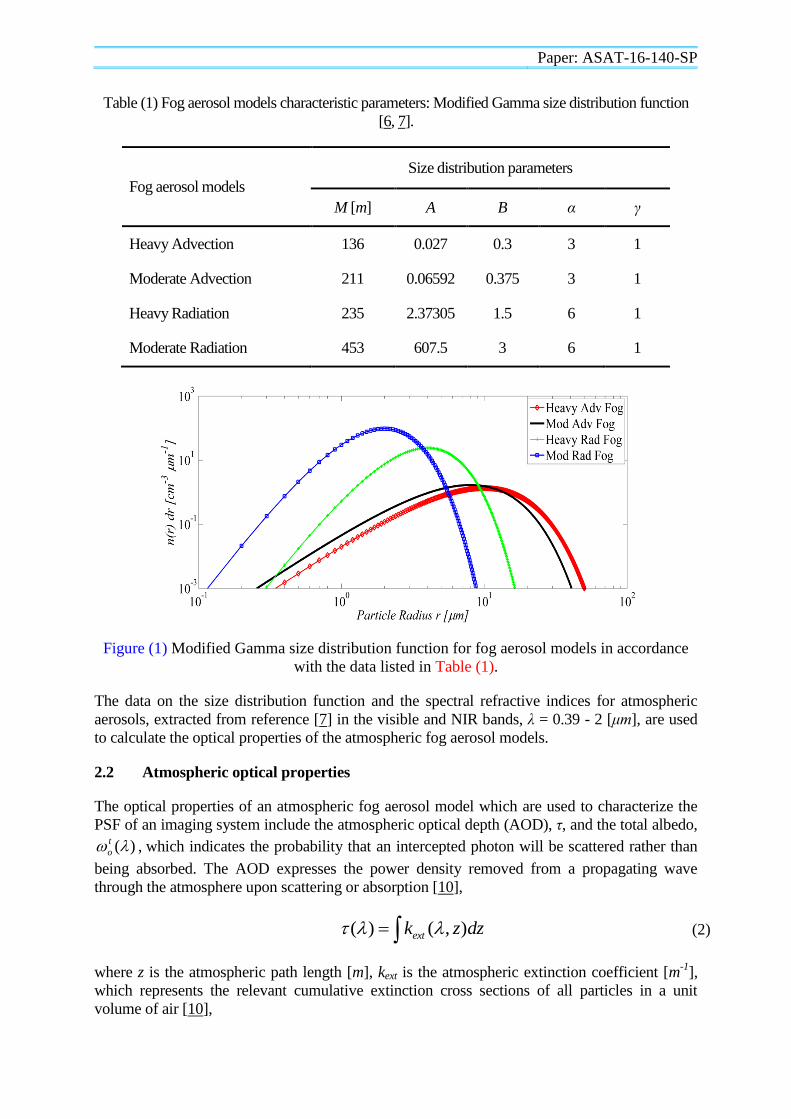
Table (1) Fog aerosol models characteristic parameters: Modified Gamma size distribution function

[6, 7].

Fog aerosol models

Size distribution parameters

M [m] A B α γ

Heavy Advection 136 0.027 0.3 3 1

Moderate Advection 211 0.06592 0.375 3 1

Heavy Radiation 235 2.37305 1.5 6 1

Moderate Radiation 453 607.5 3 6 1

Figure (1) Modified Gamma size distribution function for fog aerosol models in accordance

with the data listed in Table (1).

The data on the size distribution function and the spectral refractive indices for atmospheric

aerosols, extracted from reference [7] in the visible and NIR bands, λ = 0.39 - 2 [μm], are used

to calculate the optical properties of the atmospheric fog aerosol models.

2.2 Atmospheric optical properties

The optical properties of an atmospheric fog aerosol model which are used to characterize the

PSF of an imaging system include the atmospheric optical depth (AOD), τ, and the total albedo,

)( t

o , which indicates the probability that an intercepted photon will be scattered rather than

being absorbed. The AOD expresses the power density removed from a propagating wave

through the atmosphere upon scattering or absorption [10],

( ) ( , )extk z dz (2)

where z is the atmospheric path length [m], kext is the atmospheric extinction coefficient [m-1

],

which represents the relevant cumulative extinction cross sections of all particles in a unit

volume of air [10],

http://en.wikipedia.org/wiki/Scattering

http://en.wikipedia.org/wiki/Absorption_%28electromagnetic_radiation%29


( ) ( ) ( )ext sca absk k k (3)

where ksca and kabs are the scattering and absorption coefficients [m-1

], respectively. kext(λ),

ksca(λ), and kabs(λ) are given by [11],

0

( ) ( , ) ( )ext extk r n r dr

(4)

0

( ) ( , ) ( )sca scak r n r dr

(5)

0

( ) ( , ) ( )abs absk r n r dr

(6)

And the total albedo )( t

o is given as the ratio of ksca to kext [10, 11],

( )( )

( )

t sca

o

ext

k

k

(7)

Plots of kext(λ), kabs(λ), and ksca(λ) for the fog aerosol models, in the visible and NIR bands λ =

0.39 - 2 [μm], are shown in figure (2). The optical parameters of atmospheric fog aerosol

models for various meteorological range (M) values are calculated using our stand-alone Matlab

code, which is based on Mie scattering theory, and are listed in Table (2). These optical

properties are required to estimate the atmospheric transmittance and angular light scattering

distribution, which contribute to the PSF of an imaging system as will be clarified in the next

section.

3. Point spread function (PSF) calculation

The reduction in image quality is attributed either to reduction of image contrast, or to image

blurring. The reduction of image contrast is due to atmospheric aerosols which cause extinction

of the propagating radiation and scattering at large enough angles leading to an ultimate

reduction in the SNR. While , the image blurring is due to small-angle scattering by

atmospheric aerosols, where the scattered radiation collected by the sensor will be slightly

deviated such that fine image features such as lines and edges are blurred. This spatial effect can

be characterized as a broadening of the PSF [12]. Since the PSF is the basic physical function

that describes the spatial response of an imaging system, its calculation accounts for the effects

of the diffraction, scattering, and the appropriate optical power level of both the unscattered

(direct) and the scattered radiation arriving at the pupil of the imaging system. Since the

scattered radiation is temporally and spatially de-correlated from the direct radiation, we model

the effects of the direct (coherent) radiation and the scattered (incoherent) radiation of the

aerosol species as additive in the image plane. The angular distribution of the total detected PSF

at the image plane, PSFt(β), consists of the sum of two independent components [10, 13, 14],

t ( ) ( ) ( )dir scaPSF PSF PSF

(8)


where β [rad] is the angular distance in the image plane, PSFdir(β) is the direct PSF, or the

coherent intensity detected by the imaging system due to the direct radiation, and PSFsca(β) is

the scattered PSF, or the incoherent intensity due to the scattered radiation. Considering a plane

wave propagating in an aerosol-laden medium with path length z, and an imaging system

having focal length f and a circular entrance aperture of diameter D. In the case of an

atmospheric model with an AOD greater than 1; τ > 1, PSFdir(β) may be written as [10],

2

2

1( )2 2

dir

D kDPSF e J

f

(9)

(a) Extinction coefficient kext [km-1]

(b) Scattering coefficient ksca [km-1

]

(c) Absorption coefficient kabs [km-1

]

Figure (2) Optical properties of atmospheric fog aerosol models.


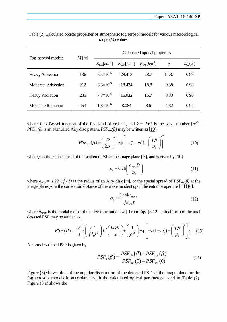
Table (2) Calculated optical properties of atmospheric fog aerosol models for various meteorological

range (M) values.

Fog aerosol models M [m]

Calculated optical properties

Kabs[km-1] Ksca [km

-1] Kext [km

-1] τ )( t

o

Heavy Advection 136 5.5×10-5

28.413 28.7 14.37 0.99

Moderate Advection 212 3.8×10-5

18.424 18.8 9.38 0.98

Heavy Radiation 235 7.8×10-6

16.032 16.7 8.33 0.96

Moderate Radiation 453 1.3×10-6

8.084 8.6 4.32 0.94

where J1 is Bessel function of the first kind of order 1, and k = 2π/λ is the wave number [m-1].

PFSdir(β) is an attenuated Airy disc pattern. PSFsca(β) may be written as [10],

2 2

( ) exp (1 )2

t

sca o

i i

D fPSF

(10)

where ρi is the radial spread of the scattered PSF at the image plane [m], and is given by [10],

0.26Airy

i

o

D

(11)

where ρAiry = 1.22 λ f / D is the radius of an Airy disk [m], or the spatial spread of PSFdir(β) at the

image plane, ρo is the correlation distance of the wave incident upon the entrance aperture [m] [10],

mod1.04 e

o

sca

a

k z (12)

where amode is the modal radius of the size distribution [m]. From Eqs. (8-12), a final form of the total

detected PSF may be written as,

22

2

12 22

1( ) exp (1 )

4 2

t

t o

ii

D e kD fPSF J

f

(13)

A normalized total PSF is given by,

( ) ( )( )

(0) (0)

dir sca

n

dir sca

PSF PSFPSF

PSF PSF

(14)

Figure (3) shows plots of the angular distribution of the detected PSFs at the image plane for the

fog aerosols models in accordance with the calculated optical parameters listed in Table (2).

Figure (3.a) shows the


(a)

(b)

(c)

Figure (3) Angular distribution of the detected PSFs for atmospheric fog aerosol models in

accordance with the calculated optical parameters listed in Table (2). Assuming an

atmospheric path length z = 500 [m], the imaging system focal length f = 10 [cm], and the

entrance aperture diameter D = 4 [cm].

(a) Direct (coherent) PSF, (b) Scattered (incoherent) PSF, (c) Normalized total PSF.

angular distribution of the direct PSF, PSFdir(β), figure (3.b) shows the radial distribution of the

scattered PSF, PSFsca(β), and figure (3.c) shows the radial distribution of the normalized total

PSF, PSFn(β). It is apparent that upon increased values of the AOD, τ, due to the various fog

aerosol models, the level of PSFdir(β) decreases significantly, whereas the level of PSFsca(β)

increases. Also, PSFdir(β) is narrowly concentrated in an Airy disc pattern, while PSFsca(β) is

widely spread throughout the entire image plane, due to the broad angle at which the scattered

light arrives at the imaging system pupil, compared to the direct light. Hence, PSFn(β) is

composed of two main components: a narrow central peak, representing the direct radiation

from the source, and a weaker wide-spread wing, representing the scattered radiation by each of


the fog models. An important conclusion is that in the central portion of the image plane, region

near β = 0, as long as PSFdir > PSFsca, it could be possible to get a reasonable image of a distant

source. However, for an increasing τ values, as PSFsca(0) approaches PSFdir(0) the image

contrast decreases gradually until the image is completely unseen for PSFsca(0) ≥ PSFdir(0). A

very important observation can be inferred from figure (3.c) is that the angular distance, β, at

which the normalized total PSF becomes approximately flat, is the angle corresponding to the

reciprocal of the cut-off frequency of an aerosol modulation transfer function (MTF).

Considering the imaging system focal length of 10 [cm]: For the heavy advection fog, moderate

advection fog, heavy radiation fog, and moderate radiation fog, β ≈ 10, 300, 500, 1000 [μrad],

respectively, which is appropriate for an MTF cut-off frequencies of 100, 3.33, 2 and 1

[cycle/mrad]. Hence, for moderate radiation fog, the PSF is about 100 times broader than that of

the heavy advection fog, and the MTF is about 100 times narrower. Aerosol MTF is thus for

heavy advection fog a high spatial frequency phenomenon [3]. This confirms the effect of

increased level of the aerosols scattered radiation on limiting the spatial resolution of an

imaging system. However, the image spectrum SNR is another metric that will confirm the

degrading effect of fog aerosols on limiting the spatial resolution of imaging systems as will be

investigated in the next section.

4. Image Spectrum Signal-to-Noise Ratio (SNR)

let I(υ) be the Fourier transform of an image which has been detected with a

photon counting camera, where υ is the spatial frequency [cycle/rad]. The image

spectrum SNR is defined as the ratio of the mean of I(υ) to the standard

deviation of I(υ) [15]. The image spectrum SNR is a measure of the relative

strengths of the image spectrum signal and the random variability of the signal

in the spatial frequency domain. Moreover, the image spectrum SNR provides a

means of estimating the noise effective resolution of an imaging system, hence

providing a useful metric of evaluating the effects of various sources of noise on

the image quality. The SNR of an image obtained with a deterministic MTF and

a photon-limited image detection system is given by [4],

,)()(

)(scadir

ndir

KK

OHKSNR

(15)

where SNR(υ) is the image spectrum SNR, H(υ) is the MTF of the imaging system, On(υ) is the

normalized Fourier spectrum of the target irradiance distribution, Kdir(λ) is the mean number of

photons directly transmitted to the imaging system from the target, and Ksca(λ) is the mean

number of photons scattered by the atmospheric aerosols before reaching the imaging system.

Kdir(λ) and Ksca(λ) are given by [4],

),(),0(

),0()(

avg

t

dirdir K

PSF

PSFK

(16)


Where PSFdir(0,λ), PSFsca(0,λ) and PSFt(0,λ) are the direct, scattered, and total effective PSF,

respectively, at the central portion of the imaging plane; PSFt(0,λ) = PSFdir(0,λ) +

PSFsca(0,λ),and Kavg(λ) is the average number of photons detected by the imaging system is

given by [4],

2

int )()()(

zch

MtAAK

opaper

avg

(18)

Where A is the area of the target [m2], Aaper = πD

2/4 [m

2], is the area of the

entrance aperture of the imaging system, τop is the optics transmittance, η is the

quantum efficiency of the detectors, tint is the integration time of the detectors

[s], M(λ) is the radiant exitance of the target in the infinitesimal wavelength

interval (λ, λ + Δλ) [Wm-2

], h is Planck's constant, h = 6.62610-34

[J.s], and c is

the speed of light, c = 3108 [m/s]. Kavg may be calculated for the visible; λc =

0.55 [μm] and NIR; λc = 1.22 [μm], spectral wavelength bands, where λc is the

central wavelength of the given spectral band, using the radiometric model

described in [4]. Also, another parameter to be defined is the noise effective

cutoff spatial frequency, υnoise [cycle/rad], of the image spectrum SNR, which is

the spatial frequency that corresponds to an image spectrum SNR value of 1.

The reciprocal of υnoise indicates a threshold noise effective spatial resolution, θth

[rad], under which the noise exceeds the signal in a given image; i.e., if the

angular spatial resolution gets smaller than θth, the noise recorded in the image

due to scattering will exceed the signal level. Figure (4) shows the radially-

averaged image spectrum SNR, SNRrad, versus the spatial frequency, υ, for the

fog aerosol models at z = 300 [m] for the fog aerosol models according to Eqs.

(15 - 18). The diffraction-limited plots, shown in figure (4), assume the absence

of atmospheric aerosols; Ksca = 0. Table (3) lists the estimated values of υnoise

[cycle/rad] and the corresponding values of θth [rad], of the image spectrum

SNR for the atmospheric aerosol models, at each spectral band as shown in

figure (4). The values of θth which is listed in Table (3) indicate that for each

atmospheric aerosol model θth at the visible spectral band is less than θth is at the

NIR spectral band, indicating a better spatial resolution of the imaging system at

shorter wavelengths, and also a better SNR. It is also noticed that for each

spectral band, θth is minimum for the moderate radiation fog aerosol model, and

θth is maximum for the heavy advection fog aerosol model, indicating a better

spatial resolution for the moderate radiation fog aerosol models, that are

characterized by a relatively lower forward-scattering, compared with the heavy

advection fog aerosol models. This notice is consistent with the values of the

meteorological ranges, M, listed in Table (2), for each atmospheric aerosol

),(),0(

),0()(

avg

t

scasca K

PSF

PSFK

(17)


model at the visible spectral band, where, as M decreases, θth increases

indicating a reduction in the image spectrum SNR [4].

(a)

(b)

Figure (4) Radially-averaged image spectrum signal-to-noise ratio, SNRrad, for the fog aerosol

models at the visible and NIR spectral wavelength bands, for an imaging system with D = 28

[cm], at z = 300 [m].

(a) Visible band (λc = 0.55 μm), (b) NIR band (λc = 1.22 μm),

Table (3) The estimated noise effective cutoff spatial frequency, υnoise [cycle/rad], of the

image-spectrum SNR for the atmospheric aerosol models, for each spectral band as shown in

figure (4), and the corresponding threshold noise effective spatial resolution, θth [rad].

Fog aerosol models

Visible spectral band

λc = 0.55 [μm]

NIR spectral band

λc = 1.22 [μm]

υnoise

[cycle/mrad]

θth

[μrad]

υnoise

[cycle/mrad]

θth

[μrad]

No aerosols 491 2.04 223.3 4.478

Moderate radiation fog 428 2.34 196.0 5.102

Heavy radiation fog 317 3.15 156.0 6.410

Heavy radiation fog 276 3.62 131.0 7.634

Heavy advection Fog 46 21.74 24.5 40.816


5. Conclusion

This paper investigates the degrading effect due to light scattering which is

provided by atmospheric fog aerosol models that can significantly affect the

quality of image acquired by electro-optical imaging systems. We clarified the

basic calculation of the atmospheric properties including the extinction

coefficient, scattering coefficient, absorption coefficient, and scattering albedo,

which contribute to the average point spread function due to various fog aerosol

models. The PSF model confirms the concentration of the coherent PSF,

resulting from the acquired direct radiation, into an attenuated Airy pattern,

whereas the incoherent PSF, that is due to the acquired scattered radiation, is

spread throughout the image plane regarding to the fact that scattering has the

effect of broadening the angle at which the scattered light arrives at the imaging

system compared to the direct light. Also, an increased atmospheric optical

depth attenuates the level of the direct PSF and increases the level of the

scattered PSF leading to a reduced image contrast. The level of the scattered

radiation relative to the level of the direct radiation coming from a source

determines the shape of the point spread function, where as long as PSFdir >

PSFsca, it could be possible to get a reasonable image quality of a distant source.

However, for an increasing atmospheric optical depth τ, the image contrast

decreases gradually until the image is completely unseen for PSFsca ≥ PSFdir.

Finally, the analysis of fog aerosol models leads to the important conclusion of

the limiting effect of aerosol scattering on the spatial resolution of the imaging

system. The other metric that emphasize the degrading effect due to fog aerosols

is the calculation of the signal-to-noise ratio recorded in a detected image and

hence, clarifies quantitatively the effect of atmospheric scattering on image

quality. We used a radiometric model for estimating the mean numbers of direct

and scattered photons detected by an imaging system from an extended target,

for a horizontal near-ground imaging scenario, upon propagation through

various fog aerosol models in the visible, and NIR spectral bands. We

incorporated the calculation of the effective PSF due to the direct and scattered

radiation acquired by an imaging system to estimate the mean numbers of direct

and scattered photons detected by an imaging system, which are then utilized to

calculate the image spectrum SNR. Finally, we demonstrated a technique for

predicting the resolution limit of an imaging system working in the presence of

fog and haze atmospheric aerosol models as a function of the optical system

parameters, the scattering medium, and the signal level which show a reduction

in the value of the noise effective spatial frequency, and consequently an

increase in the noise effective spatial resolution, for images taken through fog

aerosol media that are characterized by strong forward-scattering, hence

emphasize the degrading effect of fog aerosol models on the spatial resolution of

imaging systems operating in the visible, and NIR spectral bands.


REFERENCES

1. C. F. Bohren, and D. R. Huffman, Absorption and scattering of light by small

particles. 2004: WILEY-VCH Verlag GmbH & Co. KGaA, Weinheim.

2. N. S. Kopeika, and D. Sadot, Imaging through the atmosphere: practical

instrumentation-based theory and verification of aerosol modulation transfer function.

Journal of the Optical Society of America A, 1993. 10 (1): p. 172-179.

3. M. E. Hanafy, M. C. Roggemann, and D. O. Guney, Detailed effects of scattering and

absorption by haze and aerosols in the atmosphere on the average point spread function of an

imaging system. Journal of the Optical Society of America A, 2014. 31 (6): p. 1312 - 1319.

4. M. E. Hanafy, M. C. Roggemann, and D. O. Guney, Estimating the image

spectrumsignal-to-noise ratio for imaging through scattering media. Optical Engineering,

2015. 54 (1): p. 013102-1 - 013102-10.

5. R. C. Shirkey, and S. G. O’Brien, An Analysis of Atmospheric Aerosol Scattering for

Mid-Infrared Systems. 2006, U.S. Army Research Laboratory, White Sands Missile Range,

NM 88002-5501.

6. R. C. Shirkey, and D. H. Tofsted, High Resolution Electro-Optical Aerosol Phase

Function Database PFNDAT2006. 2008, U.S. Army Research Laboratory, White Sands

Missile Range.

7. E. P. Shettle, and R. W. Fenn, Models for the Aerosols of the Lower Atmosphere and

the Effects of Humidity Variations on Their Optical Properties. 1979, U.S. Air Force

Geophysics Laboratory, Hanscom Air Force Base, MA.

8. H. C. Hulst, Light scattering by small particles. 1981, New York: Dover Publications,

Inc.

9. K. N. Liou, An Introduction to Atmospheric Radiation. 2002: Academic Press.

10. A. Ishimaru, Wave Propagation and Scattering in Random Media. The IEEE/OUP Series,

ed. D.G. Dudley. 1997, New York: IEEE Press and Oxford University Press.

11. R. G. Grainger, Some Useful Formulae for Aerosol Size Distributions and Optical

Properties. 2012, University of Oxford.

12. M. T. Eismann, and D. A. LeMaster, Aerosol modulation transfer function model for

passive long-range imaging over a nonuniform atmospheric path. Optical Engineering, 2013.

52 (4): p. 046201-1-046201-13.

13. B. B. Dor et al., Atmospheric scattering effect on spatial resolution of imaging

systems. Journal of the Optical Society of America A, 1997. 14 (6): p. 1329-1337.

14. L. R. Bissonnette, Imaging through fog and rain. Optical Engineering, 1992. 31 (5): p.

1045-1052.

15. M. C. Roggemann, and B. M. Welsh, Imaging Through Turbelence. 1996: CRC Press.

Characterizing the Degrading Effects of Scattering by ... · forward scattering (Mie scattering)...

Documents

Transcript of Characterizing the Degrading Effects of Scattering by ... · forward scattering (Mie scattering)...