Characterizing the Codimension of Zero Singularities for ...
48
HAL Id: hal-01429961 https://hal-centralesupelec.archives-ouvertes.fr/hal-01429961 Submitted on 8 Feb 2021 HAL is a multi-disciplinary open access archive for the deposit and dissemination of sci- entific research documents, whether they are pub- lished or not. The documents may come from teaching and research institutions in France or abroad, or from public or private research centers. L’archive ouverte pluridisciplinaire HAL, est destinée au dépôt et à la diffusion de documents scientifiques de niveau recherche, publiés ou non, émanant des établissements d’enseignement et de recherche français ou étrangers, des laboratoires publics ou privés. Characterizing the Codimension of Zero Singularities for Time-Delay Systems: A Link with Vandermonde and Birkhoff Incidence Matrices Islam Boussaada, Silviu-Iulian Niculescu To cite this version: Islam Boussaada, Silviu-Iulian Niculescu. Characterizing the Codimension of Zero Singularities for Time-Delay Systems: A Link with Vandermonde and Birkhoff Incidence Matrices. Acta Applicandae Mathematicae, Springer Verlag, 2016, 145 (1), pp.47-88. 10.1007/s10440-016-0050-9. hal-01429961
Transcript of Characterizing the Codimension of Zero Singularities for ...

HAL Id: hal-01429961https://hal-centralesupelec.archives-ouvertes.fr/hal-01429961
Submitted on 8 Feb 2021
HAL is a multi-disciplinary open accessarchive for the deposit and dissemination of sci-entific research documents, whether they are pub-lished or not. The documents may come fromteaching and research institutions in France orabroad, or from public or private research centers.
L’archive ouverte pluridisciplinaire HAL, estdestinée au dépôt et à la diffusion de documentsscientifiques de niveau recherche, publiés ou non,émanant des établissements d’enseignement et derecherche français ou étrangers, des laboratoirespublics ou privés.
Characterizing the Codimension of Zero Singularities forTime-Delay Systems : A Link with Vandermonde and
Birkhoff Incidence MatricesIslam Boussaada, Silviu-Iulian Niculescu
To cite this version:Islam Boussaada, Silviu-Iulian Niculescu. Characterizing the Codimension of Zero Singularities forTime-Delay Systems : A Link with Vandermonde and Birkhoff Incidence Matrices. Acta ApplicandaeMathematicae, Springer Verlag, 2016, 145 (1), pp.47-88. 10.1007/s10440-016-0050-9. hal-01429961
Noname manuscript No.(will be inserted by the editor)
Characterizing the Codimension of Zero Singularities forTime-Delay Systems
A Link with Vandermonde and Birkhoff Incidence Matrices
Islam Boussaada · Silviu-Iulian Niculescu
Received: date / Accepted: date
Abstract The analysis of time-delay systems mainly relies on detecting andunderstanding the spectral values bifurcations when crossing the imaginaryaxis. This paper deals with the zero singularity, essentially when the zero spec-tral value is multiple. The simplest case in such a configuration is characterizedby an algebraic multiplicity two and a geometric multiplicity one, known asthe Bogdanov-Takens singularity. Moreover, in some cases the codimension ofthe zero spectral value exceeds the number of the coupled scalar-differentialequations. Nevertheless, to the best of the author’s knowledge, the boundsof such a multiplicity have not been deeply investigated in the literature. Itis worth mentioning that the knowledge of such an information is crucial fornonlinear analysis purposes since the dimension of the projected state on thecenter manifold is none other than the sum of the dimensions of the generalizedeigenspaces associated with spectral values with zero real parts. Motivated bya control-oriented problems, this paper provides an answer to this question fortime-delay systems, taking into account the parameters’ algebraic constraintsthat may occur in applications. We emphasize the link between such a problemand the incidence matrices associated with the Birkhoff interpolation problem.In this context, symbolic algorithms for LU-factorization for functional con-fluent Vandermonde as well as some classes of bivariate functional Birkhoffmatrices are also proposed.
I. BoussaadaLaboratoire des Signaux et Systemes, Universite Paris SaclayCNRS-CentraleSupelec-Universite Paris Sud3 rue Joliot-Curie, 91192 Gif-sur-Yvette cedex (France) &IPSA, 7 rue Maurice Grandcoing, 94200 Ivry-sur-Seine (France)E-mail: [email protected]
S-I. NiculescuLaboratoire des Signaux et Systemes, Universite Paris SaclayCNRS-CentraleSupelec-Universite Paris Sud3 rue Joliot-Curie, 91192 Gif-sur-Yvette cedex (France)E-mail: [email protected]

2 Islam Boussaada, Silviu-Iulian Niculescu
Keywords Time-Delay · Stability · Center Manifold · Bifurcation Anal-ysis · Bogdanov-Takens Singularity · Vandermonde Matrix · MultivariatePolynomial Interpolation · Birkhoff Matrix · LU-Factorization · RecurrenceRelation · Differential Relation
Contents
1 Introduction . . . . . . . . . . . . . . . . . . . . . . . . . . . . . . . . . . . . . . . . 2
2 Prerequisites and statement of the problem . . . . . . . . . . . . . . . . . . . . . . 6
3 Motivating examples and further observations . . . . . . . . . . . . . . . . . . . . . 11
4 LU-factirization for some classes of functional Birkhoff matrices . . . . . . . . . . 15
5 Codimension of zero Singularities of TDS . . . . . . . . . . . . . . . . . . . . . . . 23
6 Illustrative examples: An effective approach vs Polya-Szego Bound . . . . . . . . . 26
7 Concluding remarks and future work . . . . . . . . . . . . . . . . . . . . . . . . . . 33
1 Introduction
1
Matrices arising from a wide range of problems in mathematics and engi-neering typically display a characteristic structure. Exploiting such a structureis the means to the design of efficient algorithms, see for instance [3]. This studyis a crossroad between the investigation of a class of such structured matricesoriginally involved in Multivariate Interpolation Problems (namely, the well-known Birkhoff Interpolation Problem) and the estimation of the upper boundfor the codimension of spectral values of linear Time-Delay Systems (TDS)(which are the zeros of some characteristic entire function called characteristicquasipolynomial). The aim of this paper is three fold: firstly, it emphasizes thelink between the above two quoted issues. Secondly, it shows that the codi-mension of the zero spectral value of a given TDS is characterized by somealgebraic properties of an appropriate functional Birkhoff Matrix. Finally, itshows the effectiveness of the proposed constructive approach by exploring thegeneric settings as well as investigating some specific but significant sparsitypatterns. In both cases, symbolic algorithms for LU-factorization are estab-lished for some novel classes of Birkhoff matrices. It is worth mentioning thatsuch an attempt can be exploited for further classes of Birkhoff matrices andshould be of interest in some linear algebra problems involving structuredmatrices as well as in applications including polynomial interpolation.
The class of systems considered throughout this paper is infinite-dimensionalwith N discrete (constant) delays. Let z = (z1, . . . , zn) ∈ Rn denote the state-vector, then the system reads as follows
1 Some of the results proposed in this work have been presented in The 13th EuropeanControl Conference, June 24-27, 2014, Strasbourg, France [1] and The 21st InternationalSymposium on Mathematical Theory of Networks and Systems July 7-11, 2014, Groningen,The Netherlands [2]
Characterizing the Codimension of Zero Singularities for Time-Delay Systems 3
z =
N∑k=0
Akz(t− τk), (1)
under appropriate initial conditions belonging to the Banach space of con-tinuous functions C([−τN , 0],Rn). Here τk, k = 1 . . . N are strictly increas-ing positive constant delays such that τ0 = 0 and τ = (τ1, . . . , τN ), andAk ∈ Mn(R) for k = 0 . . . N . It is well known that the exponential sta-bility of the solutions of (1) is derived by the location of the spectrum χ,where χ designates the set of roots of the characteristic function [4,?]. Noticethat such a function, denoted in the sequel ∆(λ, τ), is transcendental in theLaplace variable λ. Such a spectrum χ can be split as χ = χ+∪χ0∪χ− whereχ+ = λ ∈ C, ∆(λ, τ) = 0, <(λ) > 0, χ− = λ ∈ C, ∆(λ, τ) = 0, <(λ) < 0and χ0 = λ ∈ C, ∆(λ, τ) = 0, <(λ) = 0. More precisely, the characteristicfunction of system (1) ∆ : C× RN+ → C which reads as
∆(λ, τ) = det
(λ I −A0 −
N∑k=1
Ak e−τkλ
), (2)
One can prove that the quasipolynomial function (2) admits an infinite num-ber of zeros, see for instance the references [5,6,7]. The study of zeros of anentire function [7] of the form (2) plays a crucial role in the analysis of asymp-totic stability of the zero solution of some given system (1). Indeed, the zerosolution is asymptotically stable if all the zeros of (2) are in the open left-halfcomplex plane [8]. Accordingly to this observation, the parameter space whichis spanned by the coefficients of the polynomials Pi, can be split into domains,each of them with a constant number of right half-plane characteristic roots(which is nothing but the so-called D-decomposition, see for instance [8] andreferences therein). These domains are separated by a boundary correspondingto the case when at least one characteristic root belongs to the spectrum. Inthe stability analysis of TDS, we are particularly interested by the stabilitydomains (all characteristic roots with strictly negative real parts) as well astheir boundary. Moreover, under appropriate algebraic restrictions, a givenroot associated to such a boundary may have high codimension. In this paper,we are concerned with the codimension of the zero spectral value. The typicalexample for non-simple zero spectral value is the Bogdanov-Takens singularitywhich is characterized by an algebraic multiplicity two and a geometric mul-tiplicity one. Cases with higher order multiplicities of the zero spectral valueare known to us as generalized Bogdanov-Takens singularities. Those types ofconfigurations are not only theoretical and are involved in concrete applica-tions. Indeed, the Bogdanov-Takens singularity is identified in [9] where thecase of two coupled scalar delay equations modeling a physiological controlproblem is studied. In [10] and [11] this type of singularity is also encoun-tered in the study of coupled axial-torsional vibrations of some oilwell rotarydrilling system. Moreover, the paper [12] is devoted to the analysis of such typeof singularities where codimension two and three are studied, and the associ-ated center manifolds are explicitly computed. It is commonly accepted that

4 Islam Boussaada, Silviu-Iulian Niculescu
the time-delay induces desynchronizing and/or destabilizing effects on the dy-namics. However, new theoretical developments in control of finite-dimensionaldynamical systems suggest the use of delays in the control laws for stabiliza-tion purposes. For instance, [13,14] are concerned by the stabilization of theinverted pendulum by delayed control laws and provide concrete situationswhere the codimension of the zero spectral value exceeds the number of thecoupled scalar equations modeling the inverted pendulum on cart. In [13], theauthors prove that the delayed proportional-derivative (PD) controller stabi-lizes the inverted pendulum by identifying a codimension three singularity fora system of two coupled delay equations. In [14], the same singularity is char-acterized by using a particular delay block configuration. It is shown that twodelay blocks offset a PD delayed controller.
Although the algebraic multiplicity of each spectral value of a time-delaysystem is finite (a direct consequence of Rouche lemma, see [15]), to the bestof the author’s knowledge, the computation of the upper bound of the codi-mension of the zero spectral value did not receive a complete characterizationespecially in the case when the physical parameters of a given time-delay modelare subject to algebraic constraints. Namely, if the root at the origin is invari-ant with respect to the delay parameters, however, its multiplicity is stronglydependent on the existing links between the delays and the other parametersof the system.
Furthermore, the knowledge of the codimension of such a spectral value aswell as the number of purely imaginary spectral values counting their multiplic-ities are valuable information. For instance, such an information allows to esti-mate the number of unstable roots; card(χ+) where χ+ = λ ∈ C, ∆(λ, τ) =0, <(λ) > 0 for a given time-delay system (1). Actually, the main theo-rem from [16, p. 223], which is reported in the Appendix, emphasizes the linkbetween card(χ+) and card(χ0) (Multiplicity is taken into account). In thelight of the quoted result and its potential consequences on designing new ap-proaches for the characterization of the linear stability analysis of time-delaysystems, the need of for greater emphasis on the study of the zero singularityand, more generally, the imaginary roots becomes obvious. Finally, it is worthmentioning that such a study is also interesting from a nonlinear analysis view-point, which gives another motivation for the present investigation. When theunstable spectrum is an empty set or equivalently χ = χ− ∪ χ0, a completeknowledge of the imaginary roots as well as their multiplicities becomes crucialpredominatingly when the center manifold and the normal forms theory areinvolved for deriving an accurate local qualitative description of the studieddynamical system, see [17]. In particular, in this case, when the zero spectralvalue is the only spectral value with zero real part; χ0 = 0, then the cen-ter manifold dimension is none other than the codimension of the generalizedBogdanov-Takens singularity [18,17,19].
In the context mentioned above, as a first estimation on the bound forthe codimension of the zero spectral value for quasipolynomial functions, weemphasize the Polya-Szego bound [15, pp. 144], which will be denoted ]PSin the sequel. The proof of such a result is based on the Rouche lemma and
Characterizing the Codimension of Zero Singularities for Time-Delay Systems 5
Cauchy’s argument principle, see also [20, pp. 198] for further insights on thedistribution of zeros of quasipolynomial functions. Recall that ]PS bound isnothing but the degree of the considered quasipolynomial function, see also[21] for a modern formulation of the mentioned result. Originally, the Polya-Szego result, which is reported in the Appendix, gives a bound for the numberof roots of a quasipolynomial function in a horizontal strip α ≤ I(z) ≤ β. Set-ting α = β = 0 provides a bound for the number of real spectral values, whichis a natural bound for the multiplicity of the zero spectral value. It will bestressed in the sequel that the Polya-Szego bound is a sharp bound for the zerospectral value multiplicity in the case of quasipolynomial functions consistingin the so-called complete or dense polynomials. Nevertheless, it is obvious thatthe Polya-Szego bound remains unchanged when certain coefficients ci,j vanishwithout affecting the degree of the quasipolynomial function. Such a simpleremark allows us claiming that Polya-Szego bound does not take into accountthe algebraic constraints on the parameters. However, such constraints appearnaturally in applications. In fact, models issued from applications often con-sist in lacunary ou sparse structures [22], illustrative examples will be given inthe next section concerned by motivations. Moreover, when one needs condi-tions insuring a given multiplicity bounded by ]PS , then computations of thesuccessive differentiations of the quasipolynomial have to be made.
In the sequel, among others, we emphasize a systematic approach allowingto a sharper bound for the zero spectral value multiplicity. Indeed, the pro-posed approach does not only take into account the algebraic constraints onthe coefficients ci,j but it also gives appropriate conditions guaranteeing anyadmissible multiplicity. Furthermore, the symbolic approach we adopt in thisstudy underlines the connection between the codimension of the zero singular-ity problem and incidence matrices of the so-called Confluent VandermondeMatrix as well as the Birkhoff Matrix, see for instance [23,24,25,26]. To thebest of the author’s knowledge, the first time the Vandermonde matrix appearsin a control problem is reported in [27, p. 121], where the controllability of afinite dimensional dynamical system is guaranteed by the invertibility of sucha matrix, see also [28,29]. Next, in the context of time-delay systems, the useof the standard Vandermonde matrix properties was proposed by [30,8] whencontrolling one chain of integrators by delay blocks. Here we further exploitthe algebraic properties of such matrices into a different context.
The remaining paper is organized as follows. Section 2 presents some pre-requisites and the problem statement. It is concluded by a more focused de-scription of the paper objectives and contributions. Section 3 exhibits some mo-tivating examples including some illustrations of the limitations of the Polya-Szego bound ]PS . Next, the main results are proposed and proved in Section4 and Section 5. Namely, Section 4 provides some symbolic algorithms forthe LU-factorisation associated to some classes of functional Birkhoff Matri-ces. Then, the results of the later section are exploited in Section 5 whichprovides an adaptive bound for the multiplicity of the zero spectral value forquasipolynomial functions. Various illustrative examples and control-oriented
6 Islam Boussaada, Silviu-Iulian Niculescu
discussions are presented in Section 6. Finally, some concluding remarks endthe paper.
2 Prerequisites and statement of the problem
Let us start by setting a new parametrization for the quasipolynomial function(2) characterizing the time-delay system (1) and defining some useful notationsadopted through the paper.
Some straightforward computations give the following formal expression ofthe quasipolynomial function (2)
∆(λ, σ) = P0(λ) +∑
Mk∈SN,n
PMk(λ) eσMk λ, (3)
where σMk = −Mk τT and SN,n is the set of all the possible row vectorsMk = (Mk
1 , . . . , MkN ) belonging to NN such that 1 ≤Mk
1 +. . .+MkN ≤ n. Fur-
thermore, by running the index from 1 to the cardinality NN,n , card(SN,n)the quasipolynomial (3) is written in the following compact form
∆(λ, σ) = P0(λ) +
NN,n∑k=1
Pk(λ) eσk λ. (4)
For instance,
S3,2 = (1, 0, 0), (0, 1, 0), (0, 0, 1), (2, 0, 0), (1, 1, 0), (1, 0, 1), (0, 2, 0),
(0, 1, 1), (0, 0, 2) ,
is ordered first by increasing sums (∑Ni=1M
ki ) then by lexicographical order.
In this case one has:
M2 = (0, 1, 0) and N3,2 = 9.
A generical property of retarded systems (1) allow considering P0 as amonic polynomial of degree n in λ and the polynomials PMk satisfying deg(PMk) =
n −∑Ns=1M
ks ≤ (n − 1) ∀Mk ∈ SN,n. In the sequel, P0(λ) will be called the
delay-free polynomial and the quasipolynomial function∑NN,n
k=1 PMk(λ) eσk λ
will be called the transcendental part of the quasipolynomial.Next, let define aj,k as the coefficient of the monomial λk for the polynomial
PMj , 1 ≤ j ≤ NN,n, and denote PM0 = P0. Thus, a0,n = 1 and aj,k = 0 ∀k ≥dj = n−
∑Ns=1M
js , here dj−1 is nothing but the degree of PMj . Furthermore,
the following notations are adopted: a0 = (a0,0, a0,1, . . . , a0,n−1)T is the vec-tor of the coefficients of the delay-free polynomial and aj = (aj,0, aj,1, . . . , aj,dj−1)T
is the vector of the coefficients of the polynomial associated to the auxil-iary delay σj for 1 ≤ j ≤ NN,n. Next, set the delay auxiliary vector σ =(σ1, σ2, . . . , σNN,n
) and a = (a1/ a2/ . . . / aNN,n)T where
(x/y) = (x1, . . . , xdx , y1, . . . , ydy )T
Characterizing the Codimension of Zero Singularities for Time-Delay Systems 7
for x = (x1, . . . , xdx)T and y = (y1, . . . , ydy )T . Let us denote by ∆(k)(λ, σ) thek-th derivative of ∆(λ, σ) with respect to the variable λ. We say that zero is aneigenvalue of algebraic multiplicity/codimension m ≥ 1 for (1) if ∆(0, σ∗) =∆(k)(0, σ∗) = 0 for all k = 1, . . . ,m− 1 and ∆(m)(0, σ∗) 6= 0. We assume alsoin what follows that σk 6= σk′ for any k 6= k′ where k, k′ ∈ SN,n. Indeed, if forsome value of the delay vector τ there exists some k 6= k′ such that σk = σk′ ,then the number of auxiliary delays and the number of polynomials is reducedby considering a new family of polynomials P satisfying PMk = PMk + PMk′ .In the sequel, Dq will designate the degree of the transcendental part of thequasipolynomial. 2
Now, to characterize the structure of a given quasipolynomial function oneneeds to introduce a vector V, which will be called in the sequel incidencevector, reproducing the data on the vanishing components of the vector ”a”defined above. Thus, V is a sparsity patterns indicator for the transcendentalpart of the quasipolynomial. To do so, we introduce the symbol ”star” (?) toindicate the vanishing of a given coefficient of the transcendental part of thequasipolynomial.
To illustrate the notion of ”incidence vector” as well as the symbol ”star”,let consider the following quasipolynomial function:
∆(λ, σ) = P0(λ)+(a1,0,0,0 + a1,0,0,1λ) eσ1,0,0λ+a0,1,0,2λ2 eσ0,1,0λ+a0,0,1,1λ e
σ0,0,1λ.(5)
According to the above considerations, P0 is a polynomial with deg(P0) = n ≥3. The transcendental part of (5), is characterized by the following incidencevector
V = (x1, x1, ?, ?, x2, ?, x3). (6)
Namely, the first two components of V indicate that PM1 is a complete poly-nomial of degree 1, the three components ?, ?, x2, indicate that a0,1,0,0 =a0,1,0,1 = 0 and PM2 is a lacunary polynomial of degree 2 and finally, thelast components ?, x3 say that a0,0,1,0 and PM3 is lacunary polynomial of de-gree 1.
Let us better formalize the description of the shape of a given incidencevector. As a matter of fact, the above definition, may help in the sequel, fordescribing the organisation of the distribution of symbol ? in the componentsof the incidence vector V.
Definition 21. The symbol ? appearing in a given incidence vector V is clas-sified as follows:
– If the symbol ? (or a sequence of the symbol ?) starts a sequence of aninterpolating point xk in the incidence vector V then we call it a starterstar.
2 The sum of the degrees of the polynomials involved in the quasi-polynomial plus thenumber of polynomials involved minus one is called the degree of a given quasi-polynomial.Further discussions on such a notion can be found in [21].

8 Islam Boussaada, Silviu-Iulian Niculescu
– If the symbol ? (or a sequence of the symbol ?) is strictly included in asequence of an interpolating point xk (the symbol ? is not located at theborder of a given sequence xk) in the incidence vector V it is called anintermediate star.
– The length of a sequence of ”stars” is the number of the repetition of symbol? without interruption.
We recognize that the notion of incidence vectors we introduced above isclosely inspired from the notion of the incidence matrices. Such matrices areknown to be involved in defining the structure of the well known Birkhoffmatrices.
Initially, Birkhoff and Vandermonde matrices are derived from the problemof polynomial interpolation of some unknown function g, this can be presentedin a general way by describing the interpolation conditions in terms of inci-dence matrices, see for instance [31]. For given integers n ≥ 1 and r ≥ 0, thematrix
E =
e1,0 . . . e1,r...
...en,0 . . . en,r
is called an incidence matrix if ei,j ∈ 0, 1 for every i and j. Such a matrixcontains the data providing the known information about the function g. Letx = (x1, . . . , xn) ∈ Rn such that x1 < . . . < xn, the problem of determining apolynomial P ∈ R[x] with degree less or equal to ι (ι+1 =
∑1≤i≤n, 1≤j≤r ei,j)
that interpolates g at (x, E), i.e. which satisfies the conditions:
P (j)(xi) = g(j)(xi),
is known as the Birkhoff interpolation problem. Recall that ei,j = 1 wheng(j)(xi) is known, otherwise ei,j = 0. Furthermore, an incidence matrix E is
said to be poised if such a polynomial P is unique. This amounts to saying that,if, n =
∑ni=1
∑rj=1 ei,j then the coefficients of the interpolating polynomial P
are solutions of a linear square system with associated square matrix Υ thatwe call Birkhoff matrix in the sequel. This matrix is parametrized in x and isshaped by E . It turns out that the incidence matrix E is poised if, and onlyif, the Birkhoff matrix Υ is non singular for all x such that x1 < . . . < xn.The characterization of poised incidence matrices is solved for interpolationproblems of low degrees. As a matter of fact, the problem is still unsolved forany degree greater than six, see for instance [26,32].
Remark 1. Unlike Hermite interpolation problem, for which the knowledgeof the value of a given order derivative of the interpolating polynomial at agiven interpolating point impose the values of all the lower orders derivativesof the interpolating polynomial at that point, the Birkhoff interpolation problemrelease such a restriction. Thereby justifying the qualification of ”lacunary” todescribe the Birkhoff interpolation problem.
Characterizing the Codimension of Zero Singularities for Time-Delay Systems 9
The analogy between the introduced incidence vector V for time-delay sys-tem analysis purposes and the incidence matrix E characterizing multivariateinterpolation problems can be interpreted as follows. Each k−th row of E in-dicate the distribution of the symbol ? in the sequence of xk corresponding toV. Namely, in that row of E , each ”1” corresponds to an xk of V and each ”0”(situated at the left of at least a ”1”) corresponds to a symbol ? in V.
Proposition 21. There exists a one to one mapping between V and E.
Now, to illustrate the analogy between the two concepts of incidence vec-tor/matrix, let us consider the reduced example from [32] where the incidencematrix E is given by
E =
1 1 0 00 0 1 00 1 0 0
. (6’)
The first row of E indicates that g(x1) and g′(x1) are known. In terms oftime-delay systems purposes, this reproduces the first two components of V,namely, x1, x1. The second row of E says that only g′′(x2) is known, whichin terms of V, reproduces the components ?, ?, x2. Finally, the third row saysthat only g′(x3) is known, which reproduces the last two components ?, x3of V. This, shows that the incidence matrix (6’) and the incidence vector (6)reproduce exactly the same information. For the sake of saving space, it ismore appropriate to consider V in the sequel. Recall that one associates to(6’) (or equivalently to (6)) the following Birkhoff matrix
Υ =
1 0 0 0x1 1 0 1x21 2x1 2 2x3x31 3x21 6x2 3x23
.
Accordingly, the interpolation problem is solvable if, and only if,
12x3 x2 + 6x21 − 12x2 x1 − 6x23
does not vanish for all values of x such that x1 < x2 < x3.In the spirit of the definition of functional confluent Vandermonde matrices
introduced in [28], we provide a definition for functional Birkhoff matrices.
Definition 22. The square functional Birkhoff matrix Υ is associated to asufficiently regular function $ and an incidence matrix E (or equivalently anincidence vector V) and is defined by:
Υ = [Υ 1 Υ 2 . . . ΥM ] ∈Mδ(R) (7)
whereΥ i = [κ(ki1 )(xi) κ
(ki2 )(xi) . . . κ(kidi
)(xi)] (8)
such that kil ≥ 0 for all (i, l) ∈ 1, . . . ,M × 1, . . . , di and∑Mi=1 di = δ
whereκ(xi) = $(xi)[1 . . . x
δ−1i ]T , for 1 ≤ i ≤M. (9)

10 Islam Boussaada, Silviu-Iulian Niculescu
Remark 2. In the sequel, for the time-delay systems analysis purposes, weshall be concerned with square functional Birkhoff matrices such that $(xi) =xsi , where s is a given positive integer. Furthermore, in terms of the quasipoly-nomial function (4), the degree of the delay-free polynomial P0 is fixed thanksto the explicit choice of the function $(xi) = xsi . More precisely, n , s − 1.Analogously to the Birkhoff interpolation problem, the non degeneracy of suchfunctional Birkhoff matrices will be a fondamental assumption for investigatingthe codimension of the zero spectral values for time-delay systems.
Remark 3. When s = 0, the matrix Υ is nothing but the standard Birkhoffmatrix and thus $(xi) = 1. If, in addition, V does not contain ”stars” thenwe recover the confluent Vandermonde matrix [28]. The particular case di = 1for i = 1 . . .M corresponds to the standard Vandermonde matrix and in thiscase M = δ since Υ is assumed to be a square matrix.
The explicit development of numeric/symbolic algorithms for LU factor-ization and inversion of the confluent Vandermonde and Birkhoff matrices [29,33,34,35] is still an attracting topic due to their specific structure and theirimplications in various applications, see for instance [27,36] and referencestherein. Furthermore, in our opinion, such an objective is still challengingwhen reduced complexity algorithms are needed to factorize such matrices.For instance, the reader is referred to [29] where a numerical recipe is derivedfor computing the inversion of the confluent Vandermonde matrix with a com-putational complexity O(n2), where n corresponds to the matrix dimension.However, as emphasized in [37], deriving explicit fully analytical formulae forsuch factorizations is of great help in order to perform such efficient algorithms.
It is worth mentioning that one of the contributions of this paper is topropose an explicit recursive formula for the LU-factorization for several con-figurations of the functional Birkhoff matrix defined by (7)-(9). The proposedformulas are in the spirit of the symbolic expressions established in [35] forthe standard Vandermonde case. To the best of the author’s knowledge, suchan explicit formulas seems to be unavailable in the open literature, see e. g.,[26,35]. In fact, the historical note in [35] emphasizes that rather the extensivenumerical literature on practical solutions to Vandermonde systems fails toreveal the explicit factorization formula for the LU-factorization as well as tothe symbolic inversion of the standard Vandermonde matrix.
The functional Birkhoff matrix configurations we consider are: the firstone, no ”stars” in the incidence vector V, that is the functional confluentVandermonde matrix. Next, the second configuration is when we deal withstarter ”stars”. Finally, an LU-factorization in the case of successive interme-diate ”stars” is established. We claim that, the characterization we presentthrough the paper yields some new possibilities to get formulae in cases com-bining the two configurations (starter/intermediate ”stars”), but, this needscareful inspection of the implicated polynomials and then by adapting theproposed formula to the specific incidence vector V. Since the formulas de-pend explicitly on the choice of the specific incidence matrix E , then it makesno sense that one goes further in defining some deeper classification. Further-

Characterizing the Codimension of Zero Singularities for Time-Delay Systems 11
more, as a byproduct of the approach, we first propose a different proof for thePolya-Szego bound ]PS of the origin multiplicity deduced from proposition 72(presented in the appendix), then, we shall establish a sharper bound for sucha multiplicity under the non degeneracy condition of an appropriate Birkhoffmatrix.
To summarize, the contribution of the present paper is threefold:
1. In the general case, the Birkhoff interpolation problem may or may nothave a unique solution. To the best of the author’s knowledge, no generalpattern for its determinant is known, and thus no general formula for theinterpolating polynomial (when it exists) is known. Moreover, it seems thatthe problem is still unsolved [26,32] since such a formula depends directlyon the chosen incidence matrix among a multitude of configurations. As anattempt, we propose an explicit recursive formula for the LU-factorizationof the functional confluent Vandermonde matrix as well as some classes ofthe functional Birkhoff matrix.
2. We introduce incidence matrices for describing quasipolynomial functions.Then, we identify the existing link between the multiplicity of the zerosingularity of time-delay systems (even in the presence of coupling delays)and an appropriate functional Birkhoff matrix, as defined in Definition 22.
3. Finally, in the generic case (all the polynomials PMkk≥0 are complete),the Polya-Szego bound ]PS is completely recovered using an alternativeVandermonde-based method. Moreover, when at least one of the polyno-mials is lacunary [22] (contains a ”star” or a sequence of successive ”stars”),then under the non degeneracy of an appropriate functional Birkhoff ma-trix, we establish a bound for the multiplicity of the zero singularity whichis sharper than the Polya-Szego bound ]PS .
In order to increase the readability of the paper, the following notationsare adopted. Let ξ stand for the real vector composed from xi counting theirrepetition di through columns of Υ , that is
ξ = (x1, . . . , x1︸ ︷︷ ︸d1
, . . . , xM , . . . , xM︸ ︷︷ ︸dM
).
For instance, one has ξ1 = x1 and ξd1+d2+1 = ξd1+d2+d3 = x3. Accordingly andsetting d0 = 0, without any loss of generality, we have: ξk = ξd0+...+dr+α =ξ∑%(k)−1
l=0 dl+κ(k), where 0 ≤ r ≤ M − 1 and α ≤ dr+1; here %(k) denotes the
index of the component of x associated with ξk, that is x%(k) = ξk and byκ(k) the order of ξk in the sequence of ξ composed only by x%(k). Obviously,%(k) = r + 1 and κ(k) = α.
3 Motivating examples and further observations
3.1 A Vector Disease Model
Consider first a simple scalar differential equation with one delay representingsome biological model discussed by Cooke in [38] describing the dynamics of
12 Islam Boussaada, Silviu-Iulian Niculescu
some disease. Namely, the infected host population x(t) is governed by:
x(t) + a0 x(t) + a1 x(t− τ)− a1 x(t− τ)x(t) = 0, (10)
where a1 > 0 designates the contact rate between infected and uninfectedpopulations and it is assumed that the infection of the host recovery proceedsexponentially at a rate −a0 > 0; see also [39] for more insights on the modelingand stability results. The linearized system is given by
x(t) + a0 x(t) + a1 x(t− τ) = 0, (11)
with (a0, a1, τ) ∈ R2 ×R∗+, then the associated characteristic (transcendental)function ∆ becomes
∆(λ, τ) = λ+ a0 + a1 e−λτ , (12)
for which, the corresponding incidence vector is V = (x1).Zero is a spectral value for (11) if, and only if, ∆ vanishes at zero which is
equivalent to a0 + a1 = 0. Computations of the first derivatives of (12) withrespect to λ give, using the notation ” ∂.
∂λ = .′”,
∆′(λ, τ) = 1− τ a1 e−λτ ,∆′′(λ, τ) = τ2 a1 e
−λτ .(13)
The vanishing of the two first derivatives allows us to conclude that the codi-mension of the zero spectral value is at most two (Bogdanov-Takens singular-ity) since the algebraic multiplicity two is insured by τ = 1/a1, a0 = −a1 and∆′′(0) 6= 0 (τ ∈ R∗+).This provides the simplest example showing that the codimension of the zerospectral value can exceed the number of scalar equations defining a givensystem. Moreover, this emphasizes that the codimension of the zero singular-ity is less than the number of the free parameters involved in the associated(quasipolynomial) characteristic function. In this case, the number of free pa-rameters is three and the upper bound of the codimension is two, which isexactly the Polya-Szego bound ]PS .
3.2 Furuta Pendulum
Consider now the rotary Furuta inverted pendulum, which consists of a drivenarm that rotates in the horizontal plane and a pendulum attached to thatarm which is free to rotate in the vertical plane, see figure 1. This device hastwo rotational degrees of freedom and only one actuator and is thus an under-actuated system. Balancing the pendulum in the vertical unstable equilibriumposition requires continuous correction by a control mechanism, see [40]. Wefocus now on the use of multiple delayed proportional gain as suggested by[14] in controlling the inverted pendulum on cart. Using the Lagrange for-malism and adopting the Quanser rotary experiment settings for the physicalparameter values [41], we can easily show that the dynamics of the rotary
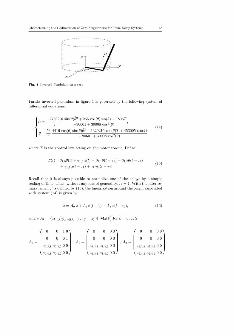
Characterizing the Codimension of Zero Singularities for Time-Delay Systems 13
Fig. 1 Inverted Pendulum on a cart
Furuta inverted pendulum in figure 1 is governed by the following system ofdifferential equations:
α = −27692
3
6 sin(θ)θ2 + 265 cos(θ) sin(θ)− 1806T
−90601 + 39008 cos2(θ),
θ =53
6
4416 cos(θ) sin(θ)θ2 − 1329216 cos(θ)T + 453005 sin(θ)
−90601 + 39008 cos2(θ),
(14)
where T is the control law acting on the motor torque. Define
T (t) =β1,0θ(t) + γ1,0α(t) + β1,1θ(t− τ1) + β1,2θ(t− τ2)
+ γ1,1α(t− τ1) + γ1,2α(t− τ2).(15)
Recall that it is always possible to normalize one of the delays by a simplescaling of time. Thus, without any loss of generality, τ1 = 1. With the later re-mark, when T is defined by (15), the linearization around the origin associatedwith system (14) is given by
x = A0 x+A1 x(t− 1) +A2 x(t− τ2), (16)
where Ak = (ak,i,j)(i,j)∈1,...,4×1,...,4 ∈M4(R) for k = 0, 1, 2
A0 =
0 0 1 0
0 0 0 1
a0,3,1 a0,3,2 0 0
a0,4,1 a0,4,2 0 0
, A1 =
0 0 0 0
0 0 0 0
a1,3,1 a1,3,2 0 0
a1,4,1 a1,4,2 0 0
, A2 =
0 0 0 0
0 0 0 0
a2,3,1 a2,3,2 0 0
a2,4,1 a2,4,2 0 0
.
14 Islam Boussaada, Silviu-Iulian Niculescu
where
a0,3,1 = −16670584
51593γ1,0, a0,3,2 = −16670584
51593β1,0 +
7338380
154779,
a0,4,1 =11741408
51593γ1,0, a0,4,2 = −24009265
309558+
11741408
51593β1,0,
a1,3,1 = −16670584
51593γ1,1, a1,3,2 = −16670584
51593β1,1, a1,4,1 =
11741408
51593γ1,1,
a1,4,2 =11741408
51593β1,1, a2,3,1 = −16670584
51593γ1,2, a2,3,2 = −16670584
51593β1,2,
a2,4,1 =11741408
51593γ1,2, a2,4,2 =
11741408
51593β1,2
System (16) is characterized by the quasipolynomial function
∆(λ, τ) =λ4 +2208852380
154779γ1,0 +
(24009265
309558− 11741408
51593β1,0 +
16670584
51593γ1,0
)λ2
+
((16670584
51593γ1,1 −
11741408
51593β1,1)λ2 +
2208852380
154779γ1,1
)e−λ
+
((−11741408
51593β1,2 +
16670584
51593γ1,2)λ2 +
2208852380
154779γ1,2
)e−λτ2 ,
(17)for which is associated the incidence vector V = (x1, ?, x1, x2, ?, x2). A zerosingularity of codimension five is insured by:
β1,0 =1710742793353
4582037506368, β1,1 =
51593
2935352, β1,2 = − 257965
10689112, τ2 =
72
265,
γ1,0 =1654329545
542135726972, γ1,1 =
29777931810
26158048826399, γ1,2 = − 438397329425
104632195305596.
(18)Also, by this example, it is easy to see that, under the delay effect, the codimen-sion of the zero singularity exceeds the dimension of the uncontrolled system(which is free of delays). Moreover, by using the Polya-Szego result, one has]PS = D−1 = 10 which is far from the effective sharp bound computationallyestablished. The bound ]PS loses its effective value due to the existence ofalgebraic constraints relating some parameters (with the notations of Propo-sition 72, c2,1 = c2,2 = c2,3 = 0. Such algebraic constraints are not taken intoaccount by the Polya-Sego approach).
3.3 Further insights on the Polya-Sego bound
As shown in the examples above, ]PS bound for the zero root multiplicity of agiven quasipolynomial function is still represents a generic bound. To be more

Characterizing the Codimension of Zero Singularities for Time-Delay Systems 15
precise, consider for instance the following three quasipolynomial functions:
∆1 =λ3 + a0,2λ2 + a0,1λ+ a0,0 +
(a1,2λ
2 + a1,1λ+ a1,0)e−λτ1
+(a2,2λ
2 + a2,1λ+ a2,0)e−λτ2 ,
∆2 =λ3 + a0,2λ2 + a0,1λ+ a0,0 +
(a1,2λ
2 + a1,1λ+ a1,0)e−λτ1
+(a2,2λ
2 + a2,0)e−λτ2 ,
∆3 =λ3 + a1,2λ2 e−λτ1 + a2,2λ
2 e−λτ2 .
(19)
It is easy to see that all of them reduce to polynomials of degree three when thedelays vanish τ1 = τ2 = 0. The quasipolynomial function ∆1 characterizes thegeneric dynamical system consisting in three coupled differential equation withtwo discrete delays. One easily observes that∆1 has complete polynomials withthe corresponding incidence vector V1 = (x1, x1, x1, x2, x2, x2), which is not thecase for the quasipolynomials ∆2 (characterized by V2 = (x1, x1, x1, x2, ?, x2))and ∆3 (characterized by V3 = (?, ?, x1, ?, ?, x2)).
Indeed, ∆2 has the so-called intermediate ”star” since the polynomial as-sociated with the second delay τ2 is sparse; a2,1 = 0. However, ∆3 has twoconnected sequences of starter ”stars”, since a2,0 = a2,1 = 0 and a1,0 = a1,1 =0 . Moreover, ]PS(∆1) = ]PS(∆2) = ]PS(∆3) because the degree of suchquasipolynomials are equal.
Nevertheless, intuitively, the multiplicity of the zero root of ∆3 is less orequal to the multiplicity of such a root for ∆1. In addition, the above ob-servation stresses the fact that the zero multiplicity depends on the numberof the free parameters as well as on the particular structure of the systemrather than on the degree of the quasipolynomial which is a generic bound ofthe number of free parameters. The next sections provide the main results ofthe paper. Section 4 provides some new LU developments for classes of func-tional Birkhoff matrices. In Section 5 , we first recover the Polya-Sego boundby an effective computational approach, then we establish a sharper boundfor the multiplicity of the zero spectral value taking into account the aboveobservation.
4 LU-factirization for some classes of functional Birkhoff matrices
In all generality, the Birkhoff interpolation problem and the ”poised”-ness ofits incidence matrices are yet open problems [26]. In some reduced cases (twovariables), related to our class of systems, we give the explicit LU-factorizationof Birkhoff matrices. To the best of the author’s knowledge, such formulae seemto be new and then it yields some new possibilities for tackling the Birkhoffinterpolation problem.
In this section we intentionally separate the two configurations: the firstone, is the regular case, that is all the polynomials of the delayed part ofthe studied quasipolynomial are complete. However, the second configurationoccurring when the incidence vector V contains at least one star.
16 Islam Boussaada, Silviu-Iulian Niculescu
4.1 On functional confluent Vandermonde matrices
It is well known that Vandermonde and confluent Vandermonde matrices Vcan be factorized into a lower triangular matrix L and an upper triangularmatrix U where V = LU , see for instance [42,43]. In what follows, we showthat the same applies for the functional confluent Vandermonde matrix (7)-(9)by establishing explicit formulas for L and U where Υ = LU . The factorizationis unique if no row or column interchanges are made and if it is specified thatthe diagonal elements of L are unitary. The following theorem concerning (7)-(9) with s = n+ 1 will be used in the sequel, but the same arguments can beeasily adapted for any positive integer s.
Theorem 41. Given the functional confluent Vandermonde matrix (7)-(9)with incidence vector V wanting ”stars” , the unique LU-factorization withunitary diagonal elements Li,i = 1 is given by the formulae:
Li,1 =xi−11 for 1 ≤ i ≤ δ,U1,j =Υ1,j for 1 ≤ j ≤ δ,Li,j =Li−1,j−1 + Li−1,j ξj for 2 ≤ j ≤ i,Ui,j =(κ(j)− 1)Ui−1,j−1 + Ui−1,j
(x%(j) − ξi−1
)for 2 ≤ i ≤ j.
(20)
Proof (Proof of Theorem 41) Define a matrix Ω by:
Ωi,j =
D∑k=1
Li,kUk,j =
i∑k=1
Li,kUk,j 1 ≤ i, j ≤ δ. (21)
In what follows, we prove that Ωi,j = Υi,j ∀(i, j) 1 ≤ i, j ≤ δ. The proof is atotal 2D recurrence-based that can be summarized as follows:
– Initialization by proving:– Ωi,j = Υi,j for i = 1 and 1 ≤ j ≤ δ that is Υ1,j .– Ωi,j = Υi,j for j = 1 and 1 ≤ i ≤ δ that is Υi,1.
– Assuming Ωi,j = Υi,j holds for any 1 ≤ i ≤ i0 − 1 and 1 ≤ j ≤ j0 − 1 andproving:– Ωi0,j0−1 = Υi0,j0−1.– Ωi0−1,j0 = Υi0−1,j0 .– Ωi0,j0 = Υi0,j0 .
– Conclude that Ωi,j = Υi,j for 1 ≤ i ≤ δ and 1 ≤ j ≤ δ
Since L is a lower triangular matrix with a unitary diagonal and U is an uppertriangular, using (20) one proves Ω1,j = U1,j ≡ Υ1,j and Ωi,1 = Li,1U1,1 ≡ Υi,1for any 1 ≤ j ≤ δ and any 1 ≤ i ≤ δ. Hence, the initialization assumptionholds. Assume now that Ωi,j = Υi,j is satisfied for any 1 ≤ i ≤ i0 − 1 and1 ≤ j ≤ j0 − 1. According to (20), one gets:
Li0,k =Li0−1,k−1 + Li0−1,k ξk,
Uk,j0−1 =(κ(j0 − 1)− 1)Uk−1,j0−2 + Uk−1,j0−1(x%(j0−1) − ξk−1
),
Characterizing the Codimension of Zero Singularities for Time-Delay Systems 17
then
Li0,kUk,j0−1 =(κ(j0 − 1)− 1)Li0−1,k−1Uk−1,j0−2 + x%(j0−1) Li0−1,k−1Uk−1,j0−1
− ξk−1 Li0−1,k−1Uk−1,j0−1 + ξk Li0−1,kUk,j0−1.
Thus,
Ωi0,j0−1 = x%(j0−1)
i0∑k=1
Li0−1,kUk,j0−1 +
i0∑k=1
(κ(j0 − 1)− 1)Li0−1,kUk,j0−2
= x%(j0−1) Υi0−1,j0−1 + (κ(j0 − 1)− 1)Υi0−1,j0−2 , Υi0,j0−1.
The same argument givesLi0−1,k =Li0−2,k−1 + Li0−2,k ξk,
Uk,j0 =(κ(j0)− 1)Uk−1,j0−1 + Uk−1,j0(x%(j0) − ξk−1
),
then
Li0−1,kUk,j0 =x%(j0) Li0−2,k−1Uk−1,j0 + (κ(j0)− 1)Li0−2,k−1Uk−1,j0−1
− ξk−1 Li0−2,k−1Uk−1,j0 + ξk Li0−2,kUk,j0 .
Thus,
Ωi0−1,j0 = x%(j0)
i0∑k=1
Li0−2,kUk,j0 +
i0∑k=1
(κ(j0)− 1)Li0−2,kUk,j0−1
= x%(j0) Υi0−2,j0 + (κ(j0)− 1)Υi0−2,j0−1 , Υi0−1,j0 .
By using again (20) one obtains:Li0,k =Li0−1,k−1 + Li0−1,k ξk,
Uk,j0 =(κ(j0)− 1)Uk−1,j0−1 + Uk−1,j0(x%(j0) − ξk−1
),
leading to:
Li0,kUk,j0 =x%(j0) Li0−1,k−1Uk−1,j0 + (κ(j0)− 1)Li0−1,k−1Uk−1,j0−1
+ ξk Li0−1,kUk,j0 − ξk−1 Li0−1,k−1Uk−1,j0 .
Hence, we have:
Ωi0,j0 = x%(j0) Υi0−1,j0 + (κ(j0)− 1)Υi0−1,j0−1 , Υi0,j0 ,
which ends the proof.
The explicit computation of the determinant of the functional confluentVandermonde matrix Υ follows directly from (20):
18 Islam Boussaada, Silviu-Iulian Niculescu
Corollary 42. The determinant of the functional confluent Vandermondematrix Υ is given by:
det(Υ ) =
δ∏j=1
(Uj,j) ,
where Uj,j for 1 ≤ j ≤ δ are defined by:
U1,1 = xn+1
1 ,
Uj,j = Uj−1,j(x%(j) − ξj−1
)if j > 1 and κ(j) = 1,
Uj,j = (κ(j)− 1)Uj−1,j−1 otherwise.
Proof Obviously, the determinant of Υ is equal to the determinant of U sincedet(L) = 1 (triangular with unitary diagonal). The second equation from (20)gives: U1,1 = xn+1
1 . Substituting i = j in the last equation from (20), andconsider j ≡ 1 mod (d0 + . . . + dr) where 1 ≤ r ≤ M that is κ(j) = 1 thenUj,j = Uj−1,j
(x%(j) − ξj−1
)otherwise x%(j) = ξj−1 which ends the proof.
Corollary 43. The diagonal elements of the matrix U associated with thefunctional confluent Vandermonde matrix Υ are obtained as follows:
U1,1 = xn+1
1 ,
Uj,j = xn+1k+1
k∏l=1
(xk+1 − xl)dl if j = 1 + dk for 1 ≤ k ≤M − 1,
Uj,j = (j − 1− dk)Uj−1,j−1 if dk + 1 < j ≤ dk+1 for 1 ≤ k ≤M − 1,
Moreover, the functional confluent Vandermonde matrix Υ is non degenerateif, and only if, ∀ 1 ≤ i 6= j ≤ δ we have xi 6= 0 and xi 6= xj.
Proof Using (20) one easily identifies the induction:
U1+dl,1+dl = (κ(1 + dl)− 1)Udl,dl + Udl,1+dl(x%(1+dl) − ξdl
)= Udl,1+dl (xl+1 − ξdl) ,
Udl,1+dl = Udl−1,1+dl (xl+1 − ξdl−1) ,
...
U2,1+dl = U1,1+dl (xl+1 − ξ1) ,
U1,1+dl = xn+1l+1 .
This ends the proof.
Characterizing the Codimension of Zero Singularities for Time-Delay Systems 19
4.2 Non degeneracy domain for two classes of 2D-functional Birkhoffmatrices: An LU-factorization
Polynomials in nature (e.g. from applications and modeling) are not necessarilygeneric. They often have some additional structure which we would like to takeinto account showing what it reflects in the multiplicity bound for the zerospectral value for time-delay systems.
In this section, we consider functional Birkhoff matrices with incidencevector V containing ”stars” . Two configurations are investigated. The firstone consists in a sequence of starter ”stars” and the second one, involves asequence of intermediate ”stars” in a sequence of xi, i > 1. We claim thatif the particular incidence matrix under study contains ”stars” in the twoconfigurations (starter/intermediate) one can benefit from the understandingof each situation separately owing the following results.
In what follows, we present an attempt to extend the results of the previoussection to the case of Birkhoff matrix (7)-(9) but with one sequence of x1wanting ”stars” and a second x2 containing ”stars” . Explicit formulas forLU -factorization will be given in two subclasses. Such developments can beeasily adapted in the study of 2D-Birkhoff interpolation problem.
We consider (7)-(9) with $(x) = xs where s = n + 1, but the same al-gorithms can be easily exploited for any functional Birkhoff matrix with thesame incidence matrix and a sufficiently regular function $, in particular,for any integer s ≥ 0. Moreover, such a restriction to the two variables casex = (x1, x2) may be extended to higher number of variables.
In terms of zeros of quasipolynomial functions, this amounts to say thatall the illustrations we provide are focused on the two-delay case.
4.2.1 Starter stars: Polynomial LU-factorization
In all generality, a functional Birkhoff matrix (7)-(9) with incidence vector
V = (x1, . . . , x1︸ ︷︷ ︸d1
, ?, . . . , ?︸ ︷︷ ︸d∗
, x2, . . . , x2︸ ︷︷ ︸d2
)
admits an LU−factorization where the associated L and U matrices are withrational coefficients in the variables x1 and x2. This claim is illustrated by thefollowing simple example.
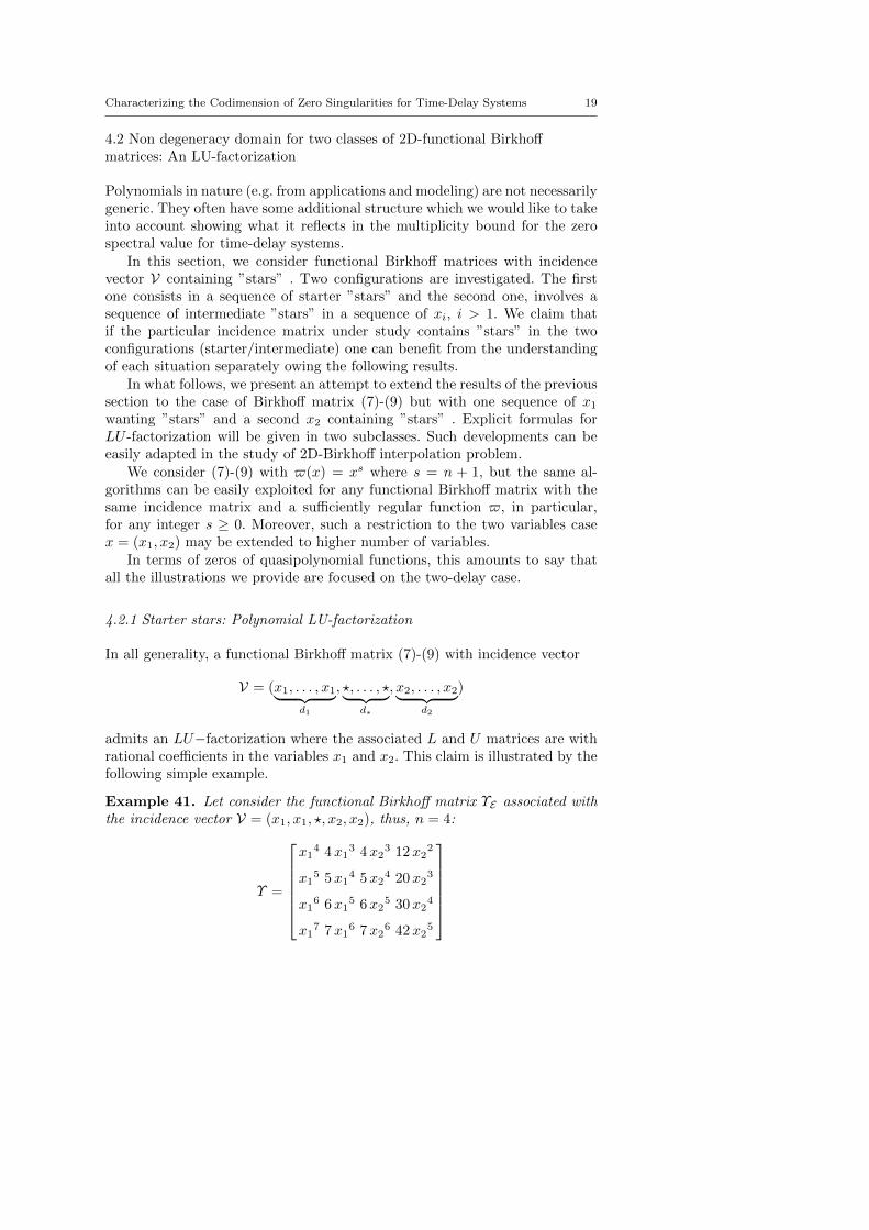
Example 41. Let consider the functional Birkhoff matrix ΥE associated withthe incidence vector V = (x1, x1, ?, x2, x2), thus, n = 4:
Υ =
x1
4 4x13 4x2
3 12x22
x15 5x1
4 5x24 20x2
3
x16 6x1
5 6x25 30x2
4
x17 7x1
6 7x26 42x2
5

20 Islam Boussaada, Silviu-Iulian Niculescu
for which one can computes the LU factorization that gives:
L =
1 0 0 0
x1 1 0 0
x12 2x1 1 0
x13 3x1
2 7 x22+7 x1x2−8 x1
2
2 (3 x2−2 x1)1
,
U =
x1
4 4x13 4x2
3 12x22
0 x14 x2
3 (5x2 − 4x1) 4x22 (5x2 − 3x1)
0 0 2x23 (3x2 − 2x1) (−x1 + x2) 2x2
2(15x2
2 + 6x12 − 20x1x2
)0 0 0
x23(−x1+x2)(10 x1
2−28 x1x2+21 x22)
3 x2−2 x1
.
Even the coefficients of L and U are rational functions in x = (x1, x2), thedeterminant of ΥE still have polynomial expression in x as expected. For in-stance, in the considered example, the denominator of U4,4 will be canceled bya factor from U3,3.
Nevertheless, there exists a unique configuration in which L and U conservetheir polynomial structure (as in the regular case), which occurs when d2 = 1independently from d1 and d∗. The following theorem provides an explicitLU−factorization for a functional Birkhoff matrix in such a special case:
Theorem 44. Given the functional Birkhoff matrix (7)-(9) with incidencevector
V = (x1, . . . , x1︸ ︷︷ ︸d1
, ?, . . . , ?︸ ︷︷ ︸d∗
, x2) (22)
the unique LU-factorization with unitary diagonal elements Li,i = 1 is givenby the formulae:
Li,1 =xi−11 for 1 ≤ i ≤ d1 + 1,
U1,j =Υ1,j for 1 ≤ j ≤ d1 + 1,
Li,j =Li−1,j−1 + Li−1,j ξj for 2 ≤ j ≤ i ≤ d1 + 1,
Ui,j =(κ(j)− 1)Ui−1,j−1 + Ui−1,j(x%(j) − ξi−1
)for 2 ≤ i ≤ j ≤ d1,
Ui,d1+1 = Υi,j − (i− 1)
∫ x1
0
Ui−1,d1+1(y, x2)dy, for 2 ≤ i ≤ d1 + 1.
(23)where ξ = (x1, . . . , x1︸ ︷︷ ︸
d1
, x2).
The proofs of Theorem 44 is provided in the appendix.
Remark 4. The proposed formulas given in Theorem 44 can be easily extendedto incidence matrices:
V = (x1, . . . , x1︸ ︷︷ ︸d1
, . . . , xn−1, . . . , xn−1︸ ︷︷ ︸dn−1
, ?, . . . , ?︸ ︷︷ ︸d∗
, xn), (24)
Characterizing the Codimension of Zero Singularities for Time-Delay Systems 21
allowing to investigate multiple zero spectral values for the n-delays case.
As a direct consequence of the above Theorem a nondegeneracy conditionis given in the following corollary:
Corollary 45. Let x1 and x2 be two distinct nonzero real numbers. TheBirkhoff matrix Υ defined by (7)-(9) with incidence vector V = (x1, . . . , x1︸ ︷︷ ︸
d1
, ?, . . . , ?︸ ︷︷ ︸d∗
, x2)
is invertible if, and only if, Ud1+1,d1+1 6= 0.
4.2.2 Intermediate stars: Polynomial LU-factorization
Similarly to the starting ”stars” case, a nondegenerate functional Birkhoffmatrix (7)-(9) with incidence vector
V = (x1, . . . , x1︸ ︷︷ ︸d1
, x2, . . . , x2︸ ︷︷ ︸d−2
, ?, . . . , ?︸ ︷︷ ︸d∗
, x2, . . . , x2︸ ︷︷ ︸d+2
)
admits an LU−factorization where the associated L and U matrices are withrational coefficients in the variables x1 and x2. Here, we provide an illustrativesimple example.
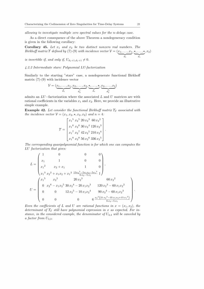
Example 42. Let consider the functional Birkhoff matrix ΥE associated withthe incidence vector V = (x1, x2, ?, x2, x2) and n = 4:
Υ =
x1
5 x25 20x2
3 60x22
x16 x2
6 30x24 120x2
3
x17 x2
7 42x25 210x2
4
x18 x2
8 56x26 336x2
5
.The corresponding quasipolynomial function is for which one can computes theLU factorization that gives:
L =
1 0 0 0
x1 1 0 0
x12 x2 + x1 1 0
x13 x2
2 + x1x2 + x12 13x2
2−5x1x2−5x12
6 x2−5 x11
,
U =
x1
5 x25 20x2
3 60x22
0 x26 − x1x25 30x2
4 − 20x1x23 120x2
3 − 60x1x22
0 0 12x25 − 10x1x2
4 90x24 − 60x1x2
3
0 0 0 6x2
4(21 x22−35 x1x2+15 x1
2)6 x2−5 x1
.
Even the coefficients of L and U are rational functions in x = (x1, x2), thedeterminant of ΥE still have polynomial expression in x as expected. For in-stance, in the considered example, the denominator of U4,4 will be canceled bya factor from U3,3.

22 Islam Boussaada, Silviu-Iulian Niculescu
The unique configuration in which L and U conserve their polynomialstructure (as in the regular case as well the stating ”stars” case with d2 =1), which occurs when d+2 = 1. The following theorem provides an explicitLU−factorization for a functional Birkhoff matrix in such a special case:
Theorem 46. Given the functional Birkhoff matrix (7)-(9) with incidencevector
V = (x1, . . . , x1︸ ︷︷ ︸d1
, x2, . . . , x2︸ ︷︷ ︸d−2
, ?, . . . , ?︸ ︷︷ ︸d∗
, x2) (25)
the unique LU-factorization with unitary diagonal elements Li,i = 1 is givenby the formulae:
Li,1 =xi−11 for 1 ≤ i ≤ d1 + d−2 + 1, (26)
U1,j =Υ1,j for 1 ≤ j ≤ d1 + d−2 + 1, (27)
Li,j =Li−1,j−1 + Li−1,j ξj for 2 ≤ j ≤ i ≤ d1 + d−2 + 1, (28)
Ui,j =(κ(j)− 1)Ui−1,j−1 + Ui−1,j(x%(j) − ξi−1
)for 2 ≤ i ≤ j ≤ d1 + d−2 ,
(29)
Ui,j =Υi,j − (i− 1)
∫ x1
0
Ui−1,j(y, x2) dy for j = d1 + d−2 + 1 and 2 ≤ i ≤ d1 + 1,
(30)
Ui,j =(j + d∗ − (i− 1))
∫ x2
0
Ui−1,j(x1, y) dy for j = d1 + d−2 + 1 and d1 + 2 ≤ i ≤ j,
(31)
where ξ = (x1, . . . , x1︸ ︷︷ ︸d1
, x2, . . . , x2︸ ︷︷ ︸d−2 +1
).
Remark 5. The proposed formulas given in theorem 46 can be easily extendedto incidence matrices:
V = (x1, . . . , x1︸ ︷︷ ︸d1
, . . . , xn−1, . . . , xn−1︸ ︷︷ ︸dn−1
, xn, . . . , xn︸ ︷︷ ︸d−n
, ?, . . . , ?︸ ︷︷ ︸d∗
, xn) (32)
As a direct consequence of the above Theorem as well as the auxiliaryLemmas 3-5 presented in the appendix, one can compute analytically the de-terminant of the considered Birkhoff matrix and then easily deduce its non-degeneracy domain. The above Corollary is in the same spirit of Corollary 42for the functional confluent Vandermonde matrices.
Corollary 47. Let x1 and x2 be two distinct nonzero real numbers. The deter-minant of the functional Birkhoff matrix Υ defined by (7)-(9) with incidencevector
V = (x1, . . . , x1︸ ︷︷ ︸d1
, x2, . . . , x2︸ ︷︷ ︸d−2
, ?, . . . , ?︸ ︷︷ ︸d∗
, x2)
Characterizing the Codimension of Zero Singularities for Time-Delay Systems 23
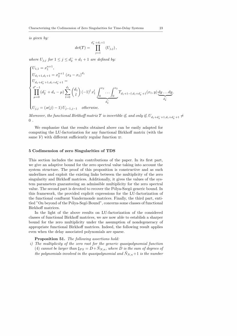
is given by:
det(Υ ) =
d−2 +d1+1∏j=1
(Uj,j) ,
where Uj,j for 1 ≤ j ≤ d−2 + d1 + 1 are defined by:
U1,1 = xn+11 ,
Ud1+1,d1+1 = xn+12 (x2 − x1)
d1
Ud1+d−2 +1,d1+d−2 +1 =
d∗−1∏µ=0
(d−2 + d∗ − µ)
d1∑l=0
(d1l
)(−1)l xl1
∫ x2
0
. . .
∫ x2
0︸ ︷︷ ︸d−2
Υd1+1−l,d1+d−2 +1(x1, y) dy . . . dy︸ ︷︷ ︸d−2
,
Uj,j = (κ(j)− 1)Uj−1,j−1 otherwise.
Moreover, the functional Birkhoff matrix Υ is invertible if, and only if, Ud1+d−2 +1,d1+d−2 +1 6=
0 .
We emphasize that the results obtained above can be easily adapted forcomputing the LU-factorization for any functional Birkhoff matrix (with thesame V) with different sufficiently regular function $.
5 Codimension of zero Singularities of TDS
This section includes the main contributions of the paper. In its first part,we give an adaptive bound for the zero spectral value taking into account thesystem structure. The proof of this proposition is constructive and as suchunderlines and exploit the existing links between the multiplicity of the zerosingularity and Birkhoff matrices. Additionally, it gives the values of the sys-tem parameters guaranteeing an admissible multiplicity for the zero spectralvalue. The second part is devoted to recover the Polya-Szego generic bound. Inthis framework, the provided explicit expressions for the LU-factorization ofthe functional confluent Vandermonde matrices. Finally, the third part, enti-tled ”On beyond of the Polya-Sego Bound”, concerns some classes of functionalBirkhoff matrices.
In the light of the above results on LU-factorization of the consideredclasses of functional Birkhoff matrices, we are now able to establish a sharperbound for the zero multiplicity under the assumption of nondegeneracy ofappropriate functional Birkhoff matrices. Indeed, the following result applieseven when the delay associated polynomials are sparse.
Proposition 51. The following assertions hold:i) The multiplicity of the zero root for the generic quasipolynomial function
(4) cannot be larger than ]PS = D+NN,n, where D is the sum of degrees of
the polynomials involved in the quasipolynomial and NN,n+1 is the number
24 Islam Boussaada, Silviu-Iulian Niculescu
of the associated polynomials. Moreover, such a bound is reached if, andonly if, the parameters of (4) satisfy simultaneously:
a0,k = −∑
i∈SN,n
(ai,k +
k−1∑l=0
ai,lσik−l
(k − l)!
), for 0 ≤ k ≤ ]PS − 1. (33)
ii Consider a quasipolynomial function (4) containing at least one incompletepolynomial for which we associate an incidence vector VE (which is nothingother than VE given by (34) where a component associated with a vanishingcoefficient is indicated by a ”star”).When the associated functional Birkhoff matrix ΥE is nonsingular, then themultiplicity of the zero root for the quasipolynomial function (4) cannot belarger than ”n” plus the number of nonzero coefficients of the polynomialfamily (PMk)Mk∈SN,n
.
Remark 6. In the generic case, the Polya-Szego bound ]PS is completely re-covered by the first assertion of 51. But, its advantage consists in providing theparameter values insuring any admissible multiplicity fo the zero singularity.The proof of Proposition 51 provides a constructive linear algebra alternativefor identifying such a bound.
Remark 7. Obviously, the number of non-zero coefficients of a given quasipoly-nomial function is bounded by its degree plus its number of polynomials. Thus,the bound elaborated in Proposition 51 ii) is sharper than ]PS, even in thegeneric case, that is all the parameters of the quasipolynomial are left free,these two bounds are equal. Indeed, in the generic case, that is when thenumber of the left free parameters is maximal, the Polya-Szego bound ]PS =D + NN,n = n + Dq + NN,n which is nothing else than n plus the number ofparameters of the polynomial family (PMk)Mk∈SN,n
.
Remark 8. When the matrix ΥE is singular, one keeps the generic Polya-Szego bound ]PS.
Remark 9. The above proposition can be interpreted as follows. Under thehypothesis:
∆(iω) = 0⇒ ω = 0 (H)
(that is, all the imaginary roots are located at the origin), the dimension ofthe projected state on the center manifold associated with zero singularity forequation (4) is less or equal to its number of nonzero coefficients minus one.Indeed, under (H), the codimension of the zero spectral value is identicallyequal to the dimension of the state on the center manifold since, in general,the dimension of the state on the center manifold is none other than the sumof the dimensions of the generalized eigenspaces associated with the spectralvalues having a zero real part.
Since we are dealing only with the values of ∆k(0), we suggest to translatethe problem into the parameter space (the space of the coefficients of the Pi).This is more appropriate and consider a parametrization by σ. In the appendix
Characterizing the Codimension of Zero Singularities for Time-Delay Systems 25
we introduce a lemma that allows to establish an m-set of multivariate alge-braic functions (polynomials) vanishing at zero when the multiplicity of thezero root of the transcendental equation ∆(λ, τ) = 0 is equal to m.
Proof (Proof of Proposition 51:) The condition (33) follows directly fromLemma 1 (see Appendix). Hereafter, we recover the bound ]PS by explicituse of functional Vandermonde matrices. Then, assuming that some coeffi-cients of the quasipolynomial vanish without affecting its degree, we showthat a sharper bound can be related to the number of nonzero parametersrather than the degree.
i) More precisely, we shall consider the variety associated with the vanish-ing of the polynomials ∇k(defined in Lemma 1 in the appendix) , thatis ∇0(0) = . . . = ∇m−1(0) = 0 and ∇m(0) 6= 0 and we aim to find themaximal m (codimension of the zero singularity).Let us exhibit the first elements from the family ∇k
∇0(0) = 0⇔NN,n∑s=0
as,0 = 0,
∇1(0) = 0⇔NN,n∑s=0
as,1 +
NN,n∑s=1
as,0 σs = 0,
∇2(0) = 0⇔ 2!
NN,n∑s=0
as,2 + 2!
NN,n∑s=1
as,1 σs +
N∑s=1
as,0 σ2s = 0.
If we consider ai,j and σk as variables, the derived algebraic system isnonlinear and solving it in all its generality (without attributing values for nand N) becomes a very difficult task. In fact, even the use of Grobner basismethods [44] seems to be very challenging since the set of variables dependson N and n. However, considering ai,j as variables and σk as parametershelps in simplifying the problem to a linear one, as seen in (33). Considerthe ideal I1 generated by polynomials < ∇0(0), ∇1(0), . . . ,∇n−1(0) > .As it can be seen from (33) and Lemma 1 (see appendix), the variety V1associated with the ideal I1 has the following linear representation a0 = Υ a
such that Υ ∈ Mn,Dq+NN,n(R[σ]) where Dq is the degree of
∑NN,n
k=1 PMk
and Dq = D − n (D the degree of the quasipolynomial (4)). Somehow,in this variety there are no restrictions on the components of a if a0 isleft free. Since a0,k = 0 for all k > n, the remaining equations consist ofan algebraic system only in a and parametrized by σ. Consider now theideal denoted I2 and generated by the Dq + NN,n polynomials defined byI2 =< ∇n+1(0), ∇n+2(0), . . . , ∇D+NN,n
(0) >. It can be observed that the
variety V2 associated with I2 can be written as Υ a = 0 which is nothing buta homogeneous linear system with Υ ∈ MDq+NN,n
(R[σ]). More precisely,
Υ is a functional confluent Vandermonde matrix (7)-(9) with x = σ, s = n,

26 Islam Boussaada, Silviu-Iulian Niculescu
M = NN,n and δ = Dq + NN,n which is associated with some incidencevector:
V = (σM1 , . . . , σM1︸ ︷︷ ︸n−
∑Ns=1M
1s
, σM2 , . . . , σM2︸ ︷︷ ︸n−
∑Ns=1M
2s
, . . . , σMNN,n
, . . . , σMNN,n
). (34)
Now, using Corollaries 42 and 43 and the assumption that σi are distinctnon zero auxiliary delays, we can conclude that the determinant of Υ cannotvanish. Thus the only solution for this subsystem is the zero solution, thatis, a = 0.Finally, consider the polynomial defined by ∇n(0), Lemma 1 states that(see appendix)
∇n(0) = 0⇔ 1 = −NN,n∑i=1
n−1∑s=0
ai,sσin−s
(n− s)!
Now, substituting the unique solution of V2 into the last equality leads toan incompatibility result. In conclusion, the maximal codimension of thezero singularity is less or equal to Dq + NN,n + n which is exactly thePolya-Szego bound ]PS = Dq + (n+ 1)︸ ︷︷ ︸
D+NN,n
proving i).
ii) She same arguments apply when z coefficients from the polynomial fam-ily (PMk)Mk∈SN,n
vanish without affecting the degree of the quasipoly-
nomial, then aT ∈ RDq+NN,n−z and thus the matrix Υ of i) becomesΥE ∈ MDq+NN,n−z(R[σ]). Thus, the invertibility of the later matrix al-lows to: the maximal codimension of the zero singularity is less or equal toDq + NN,n − z + n < ]PS . Which ends the proof.
Remark 10. It is noteworthy that the codimension of the zero singularity maydecrease if the vector parameter a0 is not left free. Indeed, if some parametercomponent a0,k is fixed for 0 ≤ k ≤ n − 1, then the variety associated to thefirst ideal I1 may impose additional restrictions on the vector parameter a.
6 Illustrative examples: An effective approach vsPolya-Szego Bound
A natural consequence of Proposition 51 is to explore the situation when thecodimension of zero singularity reaches its upper bound. Starting the sectionby a generic example, we show the convenience of the proposed approacheven in the case of cross-talk between the delays. Then the obtained sym-bolic results are applied to identify an effective sharp bound in the case ofconcrete physical system (with constraints on the coefficients). Namely, thestabilization of an inverted pendulum on cart via a multi-delayed feedback.Next, the LU-factorizations are illustrated in the two configurations starter”stars”/intermediate ”stars” and then interpreted in terms of the codimensionof the zero singularity. This section is ended by a control oriented discussion.
Characterizing the Codimension of Zero Singularities for Time-Delay Systems 27
6.1 Two scalar equations with two delays: An inverted pendulum on cartwith delayed feedback
We associate to the general planar time-delay system with two positive delaysτ1 6= τ2 the quasipolynomial function:
∆(λ, σ) =λ2 + a0,0,1λ+ a0,0,0 + (a1,0,0 + a1,0,1λ) eλσ1,0 + (a0,1,0 + a0,1,1λ) eλσ0,1
+ a2,0,0eλσ2,0 + a1,1,0eλσ1,1 + a0,2,0eλσ0,2 .(35)
Generically, the multiplicity of the zero singularity is bounded by ]PS = 9.However, in what follows, we present two configurations where such a boundcannot be reached. The first, corresponds to the case when σi = σj fori 6= j and the second, when some components of the coefficient vector a =(a1,0,0, a1,0,1, a0,1,0, a0,1,1, a2,0,0, a1,1,0, a0,2,0)T vanish.
Formula (33) allows us to explicitly computing the confluent Vandermondematrices Υ and Υ and the expression of ∇2(0) from the proof of Proposition51 such that Υ a = a0, ∇2(0) = 0 and Υ a = 0 where a0 = (a0,0,0, a0,0,1)T :
Υ =
[1 0 1 0 1 1 1
σ1,0 1 σ0,1 1 σ2,0 σ1,1 σ0,2
],
∇2(0)− 2 =[σ1,0
2 2σ1,0 σ0,12 2σ0,1 σ2,0
2 σ1,12 σ0,2
2]a
Υ =
σ1,03 3σ1,0
2 σ0,13 3σ0,1
2 σ2,03 σ1,1
3 σ0,23
σ1,04 4σ1,0
3 σ0,14 4σ0,1
3 σ2,04 σ1,1
4 σ0,24
σ1,05 5σ1,0
4 σ0,15 5σ0,1
4 σ2,05 σ1,1
5 σ0,25
σ1,06 6σ1,0
5 σ0,16 6σ0,1
5 σ2,06 σ1,1
6 σ0,26
σ1,07 7σ1,0
6 σ0,17 7σ0,1
6 σ2,07 σ1,1
7 σ0,27
σ1,08 8σ1,0
7 σ0,18 8σ0,1
7 σ2,08 σ1,1
8 σ0,28
σ1,09 9σ1,0
8 σ0,19 9σ0,1
8 σ2,09 σ1,1
9 σ0,29
.
As shown in the proof of Proposition 51, Υ is a singular matrix when σi = σjfor i 6= j. For instance, when σ2,0 = σ0,1 that is 2τ1 = τ2, then the boundof multiplicity of the zero singularity decrease since the polynomials P2,0 and
P0,1 will be collected P0,1 = P0,1 + P2,0.Consider now a system of two coupled equations with two delays modeling
a friction free inverted pendulum on cart. The adopted model is studied in [45,13,46,14] and in the sequel we keep the same notations. In the dimensionlessform, the dynamics of the inverted pendulum on a cart in figure 2 is governedby the following second-order differential equation:(
1− 3ε
4cos2(θ)
)θ +
3ε
8θ2 sin(2θ)− sin(θ) + U cos(θ) = 0, (36)
where ε = m/(m+M), M the mass of the cart and m the mass of the pendu-lum and D represents the control law that is the horizontal driving force. A

28 Islam Boussaada, Silviu-Iulian Niculescu
Fig. 2 Inverted Pendulum on a cart
generalized Bogdanov-Takens singularity with codimension three is identifiedin [13] by using U = a θ(t−τ)+b θ(t−τ). Motivated by the technological con-straints, it is suggested in [14,47] to avoid the use of the derivative gain thatrequires the estimation of the angular velocity that can induce harmful errorsfor real-time simulations and propose a multi-delayed-proportional controllerU = a1,0 θ(t− τ1) + a2,0 θ(t− τ2), this choice is argued by the accessibility ofthe delayed state by some simpler sensor. By this last controller choice and bysetting ε = 3
4 , the associated quasipolynomial function ∆ becomes:
∆(λ, τ) = λ2 − 16
7+
16 a1,07
e−λ τ1 +16 a2,0
7e−λ τ2 . (37)
Thus, the associated incidence vector is V = (x1, x2). A zero singularity withcodimension three is identified in [14], see Figure 3 for the map of local bifur-cations in the (a1,0, a2,0) plan.
Fig. 3 Bifurcations curves of (37) in the gains (a1,0, a2,0) plan (solid red=Pitchfork sin-gularity i.e. the zero singularity, discontinuous blue=Hopf singularity ) for the fixed valueτ2 = 7
8.
Characterizing the Codimension of Zero Singularities for Time-Delay Systems 29
Moreover, it is shown that the upper bound of the codimension for thezero singularity for (36) is three (can be easily checked by (33)) and thisconfiguration is obtained when the gains and delays satisfy simultaneously:
a1,0 = − 7
−7 + 8 τ1, a2,0 =
8τ12
−7 + 8 τ12, τ2 =
7
8 τ1.
However, using Polya-Szego result, one has ]PS = D−1 = (3 + 2 + 2)−1 =6 exceeding the effective bound which is three. This is a further justification forthe algebraic constraints on the parameters imposed by the physical model,for instance the sparsity pattern of the delay-free polynomial, namely, thevanishing of a0,1.
6.2 The nondegeneracy of a 2D-functional Birkhoff matrix: incidence vectorwith starter stars
As an illustration of the result given in Corollary 45, consider the functionalBirkhoff matrix Υ characterized by the incidence vector V = (x1, x1, x1, x1, x1, ?, ?, x2).Thus, one has
Υ =
x18 8x1
7 56x16 336x1
5 1680x14 56x2
6
x19 9x1
8 72x17 504x1
6 3024x15 72x2
7
x110 10x1
9 90x18 720x1
7 5040x16 90x2
8
x111 11x1
10 110x19 990x1
8 7920x17 110x2
9
x112 12x1
11 132x110 1320x1
9 11880x18 132x2
10
x113 13x1
12 156x111 1716x1
10 17160x19 156x2
11
. (38)
Under the assumptions x1x2 6= 0 and x1 6= x2, the matrix Υ is a non singularmatrix if, and only if, the bivariate polynomial 39x2
2 − 48x2x1 + 14x12 6= 0,
see Figure 4. Consider, the corresponding quasipolynomial function
∆(λ, σ) = λ7 +
6∑k=0
a0,k λk + eσ1,0λ
4∑k=0
a1,0,k λk + a0,1,2λ
2 eσ0,1λ. (39)
In terms of time-delay systems analysis purpose, the result above assertsthat if the auxiliary non zero distinct delays σ1,0 and σ0,1 satisfy 39σ0,1
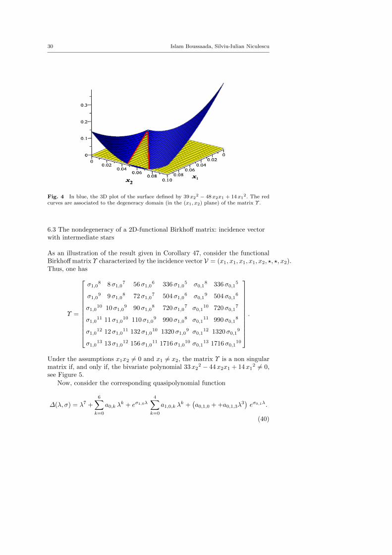
2 −48σ0,1σ1,0 + 14σ1,0
2 6= 0, then, the codimension of the zero singularity isbounded by 13. Furthermore, such a multiplicity bound is reached if, and onlyif, the parameter vectors a and a0 satisfy equality (33) for k = 0, . . . , 12. Noticethat, in this configuration, the Polya-Sego bound ]PS = 15.
30 Islam Boussaada, Silviu-Iulian Niculescu
Fig. 4 In blue, the 3D plot of the surface defined by 39x22 − 48x2x1 + 14x12. The redcurves are associated to the degeneracy domain (in the (x1, x2) plane) of the matrix Υ .
6.3 The nondegeneracy of a 2D-functional Birkhoff matrix: incidence vectorwith intermediate stars
As an illustration of the result given in Corollary 47, consider the functionalBirkhoff matrix Υ characterized by the incidence vector V = (x1, x1, x1, x1, x2, ?, ?, x2).Thus, one has
Υ =
σ1,08 8σ1,0
7 56σ1,06 336σ1,0
5 σ0,18 336σ0,1
5
σ1,09 9σ1,0
8 72σ1,07 504σ1,0
6 σ0,19 504σ0,1
6
σ1,010 10σ1,0
9 90σ1,08 720σ1,0
7 σ0,110 720σ0,1
7
σ1,011 11σ1,0
10 110σ1,09 990σ1,0
8 σ0,111 990σ0,1
8
σ1,012 12σ1,0
11 132σ1,010 1320σ1,0
9 σ0,112 1320σ0,1
9
σ1,013 13σ1,0
12 156σ1,011 1716σ1,0
10 σ0,113 1716σ0,1
10
.
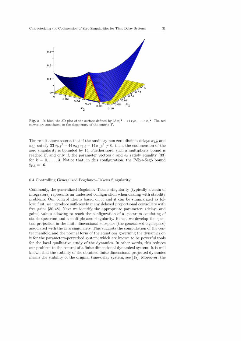
Under the assumptions x1x2 6= 0 and x1 6= x2, the matrix Υ is a non singularmatrix if, and only if, the bivariate polynomial 33x2
2 − 44x2x1 + 14x12 6= 0,
see Figure 5.
Now, consider the corresponding quasipolynomial function
∆(λ, σ) = λ7 +
6∑k=0
a0,k λk + eσ1,0λ
4∑k=0
a1,0,k λk +
(a0,1,0 + +a0,1,3λ
3)eσ0,1λ.
(40)
Characterizing the Codimension of Zero Singularities for Time-Delay Systems 31
Fig. 5 In blue, the 3D plot of the surface defined by 33x22 − 44x2x1 + 14x12. The redcurves are associated to the degeneracy of the matrix Υ .
The result above asserts that if the auxiliary non zero distinct delays σ1,0 andσ0,1 satisfy 33σ0,1
2 − 44σ0,1σ1,0 + 14σ1,02 6= 0, then, the codimension of the
zero singularity is bounded by 14. Furthermore, such a multiplicity bound isreached if, and only if, the parameter vectors a and a0 satisfy equality (33)for k = 0, . . . , 13. Notice that, in this configuration, the Polya-Sego bound]PS = 16.
6.4 Controlling Generalized Bogdanov-Takens Singularity
Commonly, the generalized Bogdanov-Takens singularity (typically a chain ofintegrators) represents an undesired configuration when dealing with stabilityproblems. Our control idea is based on it and it can be summarized as fol-low: first, we introduce sufficiently many delayed proportional controllers withfree gains [30,48]. Next we identify the appropriate parameters (delays andgains) values allowing to reach the configuration of a spectrum consisting ofstable spectrum and a multiple-zero singularity. Hence, we develop the spec-tral projection in the finite dimensional subspace (the generalized eigenspace)associated with the zero singularity. This suggests the computation of the cen-ter manifold and the normal form of the equations governing the dynamics onit for the parameters-perturbed system; which are known to be powerful toolsfor the local qualitative study of the dynamics. In other words, this reducesour problem to the control of a finite dimensional dynamical system. It is wellknown that the stability of the obtained finite dimensional projected dynamicsmeans the stability of the original time-delay system, see [18]. Moreover, the

32 Islam Boussaada, Silviu-Iulian Niculescu
matrix associated with the linear part of the finite dimensional projection ofthe parameters-perturbed system (associated with the generalized Bogdanov-Takens singularity) is nothing but a companion matrix (depending on theparameters-perturbation). It is always possible to design an appropriate per-turbation that makes this matrix Hurwitz, [30,48]. This approach proved itsefficiency particularly in suppressing undesired dynamics of mechanical sys-tems. In [45] it is shown that the only use of a proportional controller is notsufficient in stabilizing the inverted pendulum and it is proved that an addi-tional delay in the control signal is necessary for a successful stabilization. Thedescribed approach is emphasized in some recent contribution of J. Sieber & B.Krauskopf [13] for stabilizing the inverted pendulum by designing a delayed PDcontroller. Moreover, they established a linearized stability analysis allowingto characterize all the possible local bifurcations additionally to the nonlinearanalysis. This analysis involves the center manifold theory and normal forms.The study underlined the existence of a codimension-three triple zero bifur-cation. It is also shown that the stabilization of the inverted pendulum in itsupright position cannot be achieved by a PD controller when the delay exceedssome critical value τc. In [46], the authors investigate some modifications ofthe delayed PD scheme allowing to extend the range of the permissible delaysby introducing an additional parameter. For that, two options were proposed,either to additionally take into account the angular acceleration or to consideran intentional additional delay in the angular position feedback. In [14] theauthors introduce a multi-delayed-proportional controller allowing the stabi-lization of the inverted pendulum without the use of derivative measurements.Usually, the use of PD controller needs the knowledge of the velocity historybut in general we are only able to have approximate measurements due to tech-nological constraints. In absence of measurement of the derivative, a classicalidea is to use an observer to reconstruct the state, but this task is computa-tionally involved. It is shown in [47] that this type of singularity (triple zerosingularity) can be avoided by offsetting the delayed derivative gain by intro-ducing two-delayed-proportional controller. The interest of considering controllaws of the form
∑mk=1 γk x(t−τk) lies in the simplicity of the controller as well
as in its practical implementation facility, suggesting the only use of positionsensor. In a similar manner other type of singularities can be avoided. In [49],S.A. Campbell et. al. considered a proportional controller to locally maintainthe pendulum in the upright position. The authors have shown that when thisproportional is delayed and if the time-delay sampling is not too large, thecontroller still locally stabilizes the system. Among others, using the centermanifold theorem and normal forms, they show the loss of stability when thedelay exceeds a critical value and a supercritical Andronov-Hopf Bifurcation[19] occurs generating stable limit cycles. Finally, the described approach aswell as all the above cited results emphasize the importance of the imaginaryroots and motivate investigations making them more understood.

Characterizing the Codimension of Zero Singularities for Time-Delay Systems 33
7 Concluding remarks and future work
This paper addressed the problem of characterizing the dimension of theeigenspace associated with a zero singularity for time-delay systems (the ex-plicit conditions guaranteeing a given dimension) as well as an effective sharpbound for such a dimension. The existing links between the codimension of thezero singularity and functional Birkhoff matrices are emphasized. It is shownthat the codimension bound of the zero singularity relies on the number ofnonzero coefficients rather than the degree of the corresponding quasipolyno-mial. As a matter of fact, for generic quasipolynomials, a linear algebra alter-native proof for the Polya-Sego bound [15] is proposed. In the case of sparsequasipolynomials, a sharper bound for the codimension of the zero singularityis established under the non degeneracy of an appropriate functional Birkhoffmatrix. It is worth noting, that the established LU-developments yields somenew possibilities in the study of ”poised”- ness of Birkhoff incidence matri-ces. Finally, we emphasize that the proposed approach can be extended towider classes of functional equations, for instance, neutral systems and delay-difference equations. In the next step, the effect of the rational dependency ofthe delays on the codimension bound of the zero singularity will be explored.
Acknowledgements We would like to thank the anonymous Referee and theCorresponding Editor for carefully reading our manuscript and for giving com-ments and suggestions that helped improving the overall quality of the paper.We wish to thank Alban Quadrat (Inria Lille, France) for fruitful discussionson Vandermonde matrices. We would like to thank Jean-Marie Strelcyn (Uni-versite Paris 13, France) for discussions and valuable bibliographical sugges-tions. Last but not least, we thank Karim L. Trabelsi (IPSA Paris, France) forcareful reading of the manuscript and for valuable remarks.
Appendix
In this section, we first summarize the main notations in Table 1. Then, for thesake of self-containment, we report some results selected from the literature.Finally, some useful auxiliary lemmas are presented and proved. The proofs ofTheorem 44 and Theorem 46 are provided.
Here, we reporte some useful results from the mentioned literature. Themain theorem from [16] emphasizes the link between card(χ+) and card(χ0),both take into account the multiplicity.
Theorem 71 (Hassard, [16], pp. 223). Consider the quasipolynomial function∆ defined by (4). Let ρ1, . . . , ρr be the positive roots of R(y) = <(in∆(i y)),counted by their multiplicities and ordered so that 0 < ρ1 ≤ . . . ≤ ρr. For eachj = 1, . . . , r such that ∆(i ρj) = 0, assume that the multiplicity of iρj as azero of ∆(λ, τ) is the same as the multiplicity of ρj as a root of R(y). Then
34 Islam Boussaada, Silviu-Iulian Niculescu
Table 1 Table of the Main Notations
λ a complexe number.R(λ) real part of λ.I(λ) imaginary part of λ.
τ a delay vector.σ an auxiliary delay vector.z the vector state of the dynamical system.n the number of scalar differential equations defining a system.N the number of the delays involved in the dynamical system.
∆(λ, τ) a quasipolynomial function.Pi(λ) the quasipolynomial associated polynomials.al,l coefficient of λl of the l-th polynomial of ∆.χ spectrum associated to a given quasipolynomial.
χ+ the set of instable spectral values.χ− the set of stable spectral values.χ0 the set of critical spectral values i.e. crossing imaginary roots.] cardinality of a set.g unknown function to interpolate.xi interpolating points.
P interpolating polynomial.E incidence matrix.V the corresponding incidence vector.
ei,j entries of the incidence matrix.Υ a functional Birkhoff matrix corresponding to a sufficiently regular function
$.
Υ coalescence matrix associeted to Υ .
card(χ+) is given by the formula:
card(χ+) =n− card(χ0)
2+
(−1)r
2sgn I(µ)(0) +
r∑j=1
sgn I(ρj), (41)
where µ designate the multiplicity of the zero spectral value of ∆(λ, τ) = 0and I(y) = =(i−n∆(iy)). Furthermore, card(χ+) is odd (respectively, even)if ∆(µ)(0) < 0 (∆(µ)(0) > 0). If R(y) = 0 has no positive zeros, set r = 0and omit the summation term in the expression of card(χ+). If λ = 0 is nota root of the characteristic equation, set µ = 0 and interpret I(0)(0) as I(0)and ∆(0)(0) as ∆(0).
The following result from [15] gives a valuable information allowing to havea first estimation on the bound for the codimension of the zero spectral value.
Proposition 72 (Polya-Szego, [15], pp. 144). Let τ1, . . . , τN denote real num-bers such that
τ1 < τ2 < . . . < τN ,
and d1, . . . , dN positive integers satisfying
d1 ≥ 1, d2 ≥ 1 . . . dN ≥ 1, d1 + d2 + . . .+ dN = D +N.
Let fi,j(s) stands for the function fi,j(s) = sj−1 eτi s, for 1 ≤ j ≤ di and1 ≤ i ≤ N .

Characterizing the Codimension of Zero Singularities for Time-Delay Systems 35
Let ] be the number of zeros of the function
f(s) =∑
1≤i≤N,1≤j≤di
ci,j fi,j(s),
that are contained in the horizontal strip α ≤ I(z) ≤ β.Assuming that ∑
1≤k≤d1
|c1,k| > 0, . . . ,∑
1≤k≤dN
|cN,k| > 0,
then
(τN − τ1) (β − α)
2π−D + 1 ≤ ] ≤ (τN − τ1) (β − α)
2π+D +N − 1.
Setting α = β = 0, the above Proposition allows to ]PS ≤ D + N − 1where D stands for the sum of the degrees of the polynomials involved inthe quasipolynomial function f and N designate the associated number ofpolynomials. This gives a sharp bound in the case of complete polynomials.
In the sequel, we present some useful lemmas as well as the proofs of theclaimed theorems.
Lemma 1. Zero is a root of ∆(k)(λ) for k ≥ 0 if, and only if, the coefficientsof PMj for 0 ≤ j ≤ NN,n satisfy the following assertion
a0,k = −∑
i∈SN,n
[ai,k +
k−1∑l=0
ai,lσik−l
(k − l)!
]. (A.1)
Proof We define the family ∇k for all k ≥ 0 by
∇k(λ) =
NN,n∑i=0
dk
dλkPMi (λ) +
k−1∑j=0
(kj
) NN,n∑i=1
σik−j d
j
dλjPMi (λ)
, (A.2)
here, M0 , 0 and d0
dλ0 f(λ) , f(λ). Obviously, the defined family ∇k is poly-nomial since Pi and their derivatives are polynomials. Moreover, zero is a rootof ∆(k)(λ) for k ≥ 0 if, and only if, zero is a root of ∇k(λ). This can be provedby induction. More precisely, differentiating k times ∆(λ, τ) the following re-cursive formula is obtained:
∆(k)(λ) =
NN,n∑i=0
dk
dλkPMi (λ) eσiλ +
k−1∑j=0
(kj
) NN,n∑i=1
σik−j d
j
dλjPMi (λ) eσiλ
.
Since only the zero root is of interest, we can set eσiλ = 1 which define thepolynomial functions ∇k. Moreover, careful inspection of the obtained quanti-
ties presented in (A.2) and substituting dk
dλkPi(0) = k! ai,k leads to the formula(A.1).

36 Islam Boussaada, Silviu-Iulian Niculescu
Here, we prove the results given in section 4.2.1, that is, we consider theincidence vector:
V = (x1, . . . , x1︸ ︷︷ ︸d1
, ?, . . . , ?︸ ︷︷ ︸d∗
, x2).
The right hand side of the last equality from (23) defining Ui,d1+1 for 2 ≤ i ≤d1 + 1 can be also written as follows.
Lemma 2. For 2 ≤ i ≤ d1 + 1 the following equality is satisfied:
Υi,d1+1−(i−1)
∫ x1
0
Ui−1,d1+1(y, x2)dy =
i−1∑k=0
(i− 1
k
)(−1)i−1−kxi−1−k1 Υk+1,d1+1.
Proof (Proof of Lemma 2) First, one has U2,d1+1 = Υ2,d1+1 − x1 Υ1,d1+1 =Υ2,d1+1 −
∫ x1
0U1,d1+1(y, x2) dy since U1,d1+1 = Υ1,d1+1(x2).
Now, let assume that for 2 ≤ i ≤ p where p < d1 + 1 the following equalityis satisfied:
i−1∑l=0
(i− 1
l
)(−1)i−1−l xi−1−l1 Υl+1,d1+1 = Υi,d1+1−(i−1)
∫ x1
0
Ui−1,d1+1(y, x2) dy.
One has to show that for i = p+ 1:
p∑l=0
(p
l
)(−1)p−l xp−l1 Υl+1,d1+1 = Υp+1,d1+1 − (p)
∫ x1
0
Up,d1+1(y, x2) dy.
Indeed,
−∫ x1
0
pUp,d1+1(y, x2) dy = −∫ x1
0
p
p−1∑l=0
(p− 1
l
)(−1)p−1−l sp−1−l Υl+1,d1+1 ds,
= −p−1∑l=0
p!
l! (p− l − 1)!(−1)p−1−lΥl+1,d1+1
∫ x1
0
sp−1−lds,
=
p−1∑l=0
(p
l
)(−1)p−l xp−l1 Υl+1,d1+1.
Proof (Proof of Theorem 44) The only difference between algorithms (23) and(20) lies in definition of the last column of the matrix U . Thus, one has toshow that for any 2 ≤ i ≤ d1 + 1 the following equality holds Υi,d1+1 =∑ik=1 Li,kUk,d1+1. By definition, one has:
Υ2,d1+1 =
2∑k=1
L2,k Uk,d1+1
= L2,1 U1,d1+1 + L2,2 U2,d1+1
= x1 Υ1,d1+1 + U2,d1+1.
(42)
Characterizing the Codimension of Zero Singularities for Time-Delay Systems 37
Now, let assume that for 2 ≤ i ≤ p where p < d1 + 1 the following equality issatisfied:
Ui,d1+1 = Υi,d1+1 − (i− 1)
∫ x1
0
Ui−1,d1+1(y, x2) dy,
or equivalently, from Lemma 2
Ui,d1+1 =
i−1∑l=0
(i− 1
l
)(−1)i−1−l xi−1−l1 Υl+1,d1+1.
It stills to show that the last equality from (23) holds for Up+1,d1+1 whenp < d1 + 1. Indeed, by definition
Up+1,d1+1 = Υp+1,d1+1 −p∑k=1
Lp+1,kUk,d1+1.
Moreover, (for same arguments as the ones given in the proof of Lemma 6
presented in the sequel), one has Lp+1,k = 1k−1
∂Lp+1,k−1
∂x1. Thus, Lp+1,k =
1(k−1)!
∂k−1Lp+1,1
∂xk−11
= 1(k−1)!
∂k−1xp1
∂xk−11
=p! xp−k+1
1
(p−k+1)! (k−1)! . So that, one has:
Lp+1,k =
(p
k − 1
)xp−(k−1)1 . (43)
Now, by definition of Up+1,d1+1 and using (43) as well as the recurrence as-sumption, we obtain
Up+1,d1+1 = Υp+1,d1+1 −p∑l=1
Lp+1,lUl,d1+1
= Υp+1,d1+1 −p∑l=1
k−1∑l=0
(l − 1
l
)(p
l − 1
)(−1)l−l−1 xl−l−11 x
p−(l−1)1 Υl+1,d1+1
= Υp+1,d1+1 −p∑l=1
l−1∑l=0
(l − 1
l
)(p
l − 1
)(−1)l−1−l xp−l1 Υl+1,d1+1
Thus, one has to prove that
p−1∑k=0
(p
k
)(−1)p−k xp−k1 Υk+1,d1+1 = −
p∑l=1
l−1∑l=0
(l − 1
l
)(p
l − 1
)(−1)l−1−l xp−l1 Υl+1,d1+1.
(44)Recall that, the two side expressions of (44) are polynomials in x1 and x2. Theonly quantities depending in x2 are (Υk,d1+1)1≤k≤p. Since, deg(Υk,d1+1) 6=deg(Υk′,d1+1) for k 6= k′ , it will be enough to we examine the equality ofcoefficients of the two side expressions in Υm+1,d1+1 for arbitrarily chosen 0 ≤m ≤ p−1. So that, let m = k0 for which corresponds m = l0 in the right handside quantity from (44). Then consider the coefficient of xp−m1 Υm+1,d1+1 from
the two sides of (44) . Now, one easily check that∑pl=m
(l−1m
)(pl−1)
(−1)l−m
=
(−1)p−m (p
m
)is always satisfied, which ends the proof.
38 Islam Boussaada, Silviu-Iulian Niculescu
In what follow, we propose some lemmas exhibiting some interesting prop-erties of functional Birkhoff matrices. Those will be useful for the analyticalproof of Theorem 46.
Lemma 3. Equation (30) is equivalent to:
Ui,j =
i−1∑l=0
(i− 1
l
)(−1)l xl1 Υi−l,j for j = d1 + d−2 + 1 and 2 ≤ i ≤ d1 + 1.
(45)
Proof (Proof of Lemma 3) The equality (45) follows directly by induction.First, one checks that
Υ2,d1+d−2 +1 = U2,d1+d−2 +1 + x1 Υ1,d1+d−2 +1.
Indeed, Υ2,d1+d−2 +1 =
2∑k=1
L2,k Uk,d1+d−2 +1
= L2,1 U1,d1+d−2 +1 + L2,2 U2,d1+d
−2 +1
= x1 Υ1,d1+d−2 +1 + U2,d1+d−2 +1,
(46)
since L2,2 = 1. Now, let assume that
Ui,j =
i−1∑l=0
(i− 1
l
)(−1)l xl1 Υi−l,j for j = d1+d−2 +1 and 2 ≤ i ≤ p and p < d1+1,
(47)From Equation (30) one has
Up+1,d1+d−2 +1 = Υp+1,d1+d
−2 +1 − p
∫ x1
0
Up,d1+d−2 +1(y, x2)dy.
Using (47), one has,
Up+1,d1+d−2 +1
=Υp+1,d1+d−2 +1
− p∫ x1
0
(Υp,d1+d−2 +1(y, x2) +
p−1∑l=1
(p− 1
l
)(−1)l yl Υp−l,d1+d−2 +1(y, x2)
)dy
= Υp+1,d1+d−2 +1 − p Υp,d1+d−2 +1x1 +
p−1∑l=1
p
(p− 1
l
)(−1)l Υp−l,d1+d−2 +1
∫ x1
0
yl dy
=
p∑l=0
(p
l
)(−1)l xl1 Υp+1−l,d1+d−2 +1.
which ends the proof.

Characterizing the Codimension of Zero Singularities for Time-Delay Systems 39
Lemma 4.
Υi+1,j = x2 Υi,j+(d−2 +d∗)
∫ x2
0
Υi,j(y) dy for j = d1+d−2 +1 and 1 ≤ i ≤ d1+d−2 .
(48)
Proof (Proof of Lemma 4) Let consider the coalescence [50] confluent Vander-monde matrice Υ which regularize the considered Birkhoff matrice Υ . That isΥ is the rectangular matrix associated with the incidence matrix
V = (x1, . . . , x1︸ ︷︷ ︸d1
, x2, . . . , x2︸ ︷︷ ︸d−2
, x2, . . . , x2︸ ︷︷ ︸d∗
, x2).
Here, the ”stars” ? in (32) are simply replaced by x2. Thus, Υ and Υ havethe same number of rows, but the number of columns of Υ exceeds the columnsnumber of Υ by d∗. We point out that Υi+1,d1+d
−2 +1 is nothing but Υi+1,d1+d
−2 +1+d∗ .
This means that the term (d−2 + d∗)∫ x2
0Υi,j in (48) is exactly Υi+1,d1+d
−2 +d∗ .
Thus, equality (48) turns to be
Υi+1,j = x2 Υi,j + Υi,j−1 for j = d1 + d−2 + 1 + d∗ and 1 ≤ i ≤ d1 + d−2 .
This last equality can be easily proved by using a 2-D recurrence in terms ofΥ (regular matrix) as in the proof of Theorem 41 to show that it applies evenfor d1 + 2 ≤ j ≤ d1 + d−2 + 1 + d∗.
The following Lemma provides an other way defining the components of Ugiven by (30).
Lemma 5. for all i = 1, . . . , d1 and j = d1 + d−2 + 1 the following equalityapplies
Ui+1,j∗ = (x2 − x1)Ui,j∗ + (d−2 + d∗)
∫ x2
0
Ui,j∗(y)dy. (49)
Proof (Proof of Lemma 5) Let set
Ik = Uk+1,j∗ + (x1 − x2)Uk,j∗ − (d−2 + d∗)
∫ x2
0
Uk,j∗(y)dy.
where j∗ = d1 + d−2 + 1 + d∗ and 1 ≤ k ≤ d1 + 1.Substitute equation (45) from lemma 3 in Ik, to obtain
Ik =
k∑l=0
(k
l
)(−1)lxl1Υk+1−l,j∗
−k−1∑l=0
(k − 1
l
)(−1)lxl1
((x2 − x1)Υk−l,j∗ + (d−2 + d∗)
∫ x2
0
Υk−l,j∗(y)dy
).

40 Islam Boussaada, Silviu-Iulian Niculescu
Using lemma 4, one obtains
Ik =
k−1∑l=1
(−1)l xl1
[((k
l
)−(k − 1
l
))Υk+1−l,j∗ + x1
(k − 1
l
)Υk−l,j∗
]+ (−1)k xk1 Υ1,j∗ + x1 Υk,j∗
=
k−1∑l=1
(−1)l xl1
((k − 1
l − 1
)Υk+1−l,j∗ + x1
(k − 1
l
)Υk−l,j∗
)+ (−1)k xk1 Υ1,j∗
+ x1 Υk,j∗
which is as expected identically zero, that ends the proof.
The following Lemma provides a differential relation between the coeffi-cients of L matrix.
Lemma 6. for all 1 ≤ k ≤ p the following equality holds
∂Ld1+p,d1+k∂x2
= k Ld1+p,d1+k+1 (50)
The following result applies when dealing with Υi,j and Υi,j−1 are in thesame variable block. We emphasize that such a property is inherited by theexpressions of L defined in (28).
Proof (Proof of Lemma 6) The proof is 2-D recurrence-based. First, one easilycheck that for p = 2 then k = 1
Ld1+2,d1+2 =∂Ld1+2,d1+1
∂x2
since by definition of L one has Ld1+2,d1+1 = Ld1+1,d1 + x2 Ld1+1,d1+1 =
Ld1+1,d1 + x2 and∂Ld1+1,d1
∂x2= 0. When assuming that
Ld1+p,d1+2 =∂Ld1+p,d1+1
∂x2,
and again, using the definition of L, one obtains,
Ld1+p+1,d1+2 = Ld1+p,d1+1 + x2Ld1+p,d1+2,
Ld1+p+1,d1+1 = Ld1+p,d1 + x2Ld1+p,d1+1,
which as expected gives:
∂Ld1+p+1,d1+1
∂x2= Ld1+p,d1+1 + x2
∂Ld1+p,d1+1
∂x2= Ld1+p,d1+1 + x2Ld1+p,d1+2 = Ld1+p+1,d1+2.
Let assume that for any 2 < p < d−2 + 1 and k = 1, . . . , p− 1 one has
∂Ld1+p,d1+k∂x2
= k Ld1+p,d1+k+1.

Characterizing the Codimension of Zero Singularities for Time-Delay Systems 41
One has to prove the following equalities :
∂Ld1+p+1,d1+k
∂x2= k Ld1+p+1,d1+k+1,
∂Ld1+p,d1+k+1
∂x2= (k + 1)Ld1+p,d1+k+2,
∂Ld1+p+1,d1+k+1
∂x2= (k + 1)Ld1+p+1,d1+k+2.
(51)
Let us consider the first equality of (51), using the definition of L that assertsthat
Ld1+p+1,d1+k+1 = Ld1+p,d1+k + x2Ld1+p,d1+k+1
Ld1+p+1,d1+k = Ld1+p,d1+k−1 + x2Ld1+p,d1+k.
Which gives
∂Ld1+p+1,d1+k
∂x2=∂Ld1+p,d1+k−1
∂x2+ x2
∂Ld1+p,d1+k∂x2
+ Ld1+p,d1+k
= (k − 1)Ld1+p,d1+k + k Ld1+p,d1+k+1 + Ld1+p,d1+k
= k Ld1+p+1,d1+k+1.
By the same way, the remaining two equality from (51) are obtained:
∂Ld1+p,d1+k+1
∂x2=∂ (Ld1+p−1,d1+k + x2Ld1+p−1,d1+k+1)
∂x2
=∂Ld1+p−1,d1+k
∂x2+ x2
∂Ld1+p−1,d1+k+1
∂x2+ Ld1+p−1,d1+k+1
= kLd1+p−1,d1+k+1 + (k + 1)x2Ld1+p−1,d1+k+2 + Ld1+p−1,d1+k+1
= (k + 1)Ld1+p,d1+k+2,
and
∂Ld1+p+1,d1+k+1
∂x2=∂ (Ld1+p,d1+k + x2Ld1+p,d1+k+1)
∂x2
=∂Ld1+p,d1+k
∂x2+ x2
∂Ld1+p,d1+k+1
∂x2+ Ld1+p,d1+k+1
= kLd1+p,d1+k+1 + (k + 1)x2Ld1+p,d1+k+2 + Ld1+p,d1+k+1
= (k + 1)Ld1+p+1,d1+k+2.
that ends the proof.
Proof (Proof of Theorem 46) The only change occurring in (26)-(31) comparedwith (20) is the way in defining the column d1 + d−2 + 1 of U . Moreover, sucha column is only involved in computing the column d1 + d−2 + 1 of Υ . Thus, itstills to show that the equalities (30) and (31); this will be done by recurrence.Equation (30) follow directly by induction from lemma 3.
42 Islam Boussaada, Silviu-Iulian Niculescu
Let us focus now on (31) and denote j∗ = d1 + d−2 + 1. First, let us checkthat
Ud1+2,j∗ =(d−2 + d∗)
∫ x2
0
Ud1+1,j∗(x1, y) dy.
From the one side, using lemma 4 one has
Υd+2,j∗ = x2 Υd+1,j∗ + (d−2 + d∗)
∫ x2
0
Υd+1,j∗(y) dy,
= x2
d1+1∑k=1
Ld1+1,kUk,j∗ + (d−2 + d∗)
∫ x2
0
d1+1∑k=1
Ld1+1,kUk,j∗(y) dy.
Since by definition one has Ld1+1,d1+1 = 1 and Ld1+1,k = Ld1+1,k(x1) fork ∈ 1, . . . , d1 then
Υd+2,j∗ =x2
d1+1∑k=1
Ld1+1,kUk,j∗ + (d−2 + d∗)
d1∑k=1
Ld1+1,k
∫ x2
0
Uk,j∗(y)dy
+ (d−2 + d∗)
∫ x2
0
Ud1+1,j∗(y)dy.
From the other side and by definition of Υ ,
Υd1+2,j∗ =
d1+2∑k=1
Ld1+2,kUk,j∗ = Ud1+2,j∗ +
d1+1∑k=1
Ld1+2,kUk,j∗ .
To prove (31) for i = d1 + 2 one has to prove that
d1+1∑k=1
Ld1+2,kUk,j∗ = x2
d1+1∑k=1
Ld1+1,kUk,j∗ + (d−2 + d∗)
d1∑k=1
Ld1+1,k
∫ x2
0
Uk,j∗(y)dy,
or equivalently to prove
d1+1∑k=1
(Ld1+2,k − x2 Ld1+1,k)Uk,j∗ − (d−2 + d∗)
d1∑k=1
Ld1+1,k
∫ x2
0
Uk,j∗(y)dy = 0.
(52)
Using equation (28), one obtain
Ld1+2,k − x2 Ld1+1,k = Ld1+1,k−1 + (x1 − x2) Ld1+1,k, for k = 1, . . . , d1,
Ld1+2,d1+1 − x2 Ld1+1,d1+1 = Ld1+1,d1 .

Characterizing the Codimension of Zero Singularities for Time-Delay Systems 43
Thus, the right hand side of (52) becomes
d1∑k=1
Ld1+1,kUk+1,j∗ + (x1 − x2)
d1∑k=1
Ld1+1,kUk,j∗
− (d−2 + d∗)
d1∑k=1
Ld1+1,k
∫ x2
0
Uk,j∗(y)dy =
d1∑k=1
Ld1+1,k
(Uk+1,j∗ + (x1 − x2)Uk,j∗ − (d−2 + d∗)
∫ x2
0
Uk,j∗(y)dy
).
Lemma 5 asserts that for all i = 1, . . . , d1 and j = d1 + d−2 + 1 one has
Uk+1,j∗ + (x1 − x2)Uk,j∗ − (d−2 + d∗)
∫ x2
0
Uk,j∗(y)dy = 0 (53)
which implies that (31) applies for i = d1 + 2.Let assume now that, (31) is satisfied for i = d1 + 2, . . . , d1 + p where
1 < p < d−2 + d∗. It stills to prove that (31) is satisfied for i = d1 + p+ 1.By the same argument as for i = d1 + 2, one has
Υd1+p+1,j∗ =x2 Υd+p,j∗ + (d−2 + d∗)
∫ x2
0
Υd+p,j∗(y) dy,
=x2
d1+p∑k=1
Ld1+p,kUk,j∗(d−2 + d∗)
d1+p−1∑k=1
∫ x2
0
Ld1+p,kUk,j∗(y)dy
+ (d−2 + d∗)
∫ x2
0
Ud1+p,j∗(y)dy
=x2
d1+p∑k=1
Ld1+p,kUk,j∗ + (d−2 + d∗)
d1+p−1∑k=1
∫ x2
0
Ld1+p,kUk,j∗(y)dy
+ (p− 1)
∫ x2
0
Ud1+p,j∗(y)dy + (d−2 + d∗ − p+ 1)
∫ x2
0
Ud1+p,j∗(y)dy
From the other side, we obtain
Υd1+p+1,j∗ =
d1+p∑k=1
Ld1+p+1,kUk,j∗ + Ud1+p+1,j∗ .
Hence, we have to prove that
d1+p∑k=1
Ld1+p+1,kUk,j∗ − x2d1+p∑k=1
Ld1+p,kUk,j∗ − (d−2 + d∗)
d1+p−1∑k=1
∫ x2
0
Ld1+p,kUk,j∗(y)dy
= (p− 1)
∫ x2
0
Ud1+p,j∗(y)dy.
44 Islam Boussaada, Silviu-Iulian Niculescu
Now, using the result from Lemma 5, one has to prove that
d1+p∑k=d1+2
Ld1+p+1,kUk,j∗ − x2d1+p∑k=d1+2
Ld1+p,kUk,j∗ (54)
− (d−2 + d∗)
d1+p−1∑k=d1+1
∫ x2
0
Ld1+p,kUk,j∗(y)dy (55)
= (p− 1)
∫ x2
0
Ud1+p,j∗(y)dy. (56)
Using equation (28), one obtains
Ld1+p+1,k − x2 Ld1+p,k = Ld1+p,k−1, for k = d1 + 2, . . . , d1 + p.
Finally, equation (54) becomes
E =
p−1∑k=1
Ld1+p,d1+kUd1+k+1,j∗ − (d−2 + d∗)
p−1∑k=1
∫ x2
0
Ld1+p,d1+kUd1+k,j∗(y)dy
− (p− 1)
∫ x2
0
Ud1+p,j∗(y)dy = 0.
(57)Differentiating E given in (57) with respect to the variable x2 one obtains
∂E
∂x2=
p−1∑k=1
(∂Ld1+p,d1+k
∂x2Ud1+k+1,j∗ + Ld1+p,d1+k
∂Ud1+k+1,j∗
∂x2
)
− (d−2 + d∗)
p−1∑k=1
Ld1+p,d1+kUd1+k,j∗ − (p− 1)Ud1+p,j∗
=
p−1∑k=1
∂Ld1+p,d1+k∂x2
Ud1+k+1,j∗
+
p−1∑k=1
Ld1+p,d1+k
(∂Ud1+k+1,j∗
∂x2− (d−2 + d∗)Ud1+k,j∗
)− (p− 1)Ud1+p,j∗
Characterizing the Codimension of Zero Singularities for Time-Delay Systems 45
By using the recurrence assumption, one obtains,
∂E
∂x2=
p−1∑k=1
∂Ld1+p,d1+k∂x2
Ud1+k+1,j∗ − (p− 1)Ud1+p,j∗
+
p−1∑k=1
Ld1+p,d1+k((d−2 + d∗ − (k − 1))Ud1+k,j∗ − (d−2 + d∗)Ud1+k,j∗
)=
p−1∑k=1
∂Ld1+p,d1+k∂x2
Ud1+k+1,j∗ −p−1∑k=2
(k − 1)Ld1+p,d1+k Ud1+k,j∗ − (p− 1)Ud1+p,j∗
=
p−2∑k=1
(∂Ld1+p,d1+k
∂x2− k Ld1+p,d1+1+k
)Ud1+1+k,j∗
+
(∂Ld1+p,d1+p−1
∂x2− (p− 1)
)Ud1+p,j∗ ≡ 0,
which is as expected zero since Lemma 6 asserts that each factor is identicallyzero, that ends the proof.
References
1. I. Boussaada, D. Irofti, S.-I. Niculescu, Computing the codimension of the singularity atthe origin for delay systems in the regular case: A vandermonde-based approach, 13thEuropean Control Conference June 24-27, 2014. Strasbourg, France (2014) 97–102.
2. I. Boussaada, S.-I. Niculescu, Computing the codimension of the singularity at the originfor delay systems: The missing link with birkhoff incidence matrices, 21st InternationalSymposium on Mathematical Theory of Networks and Systems July 7-11, 2014. Gronin-gen, The Netherlands (2014) 1699–1706.
3. D. Bini, P. Boito, A fast algorithm for approximate polynomial gcd based on structuredmatrix computations, in: D. Bini, V. Mehrmann, V. Olshevsky, E. Tyrtyshnikov, M. vanBarel (Eds.), Numerical Methods for Structured Matrices and Applications, Vol. 199 ofOperator Theory: Advances and Applications, Birkhauser Basel, 2010, pp. 155–173.
4. O. Diekmann, S. V. Gils, S. V. Lunel, H. Walther, Delay equations, Vol. 110 of AppliedMathematical Sciences, Functional, complex, and nonlinear analysis, Springer-Verlag,New York, 1995.
5. R. Bellman, K. L. Cooke, Differential-difference equations, Academic Press, New York,1963.
6. L. V. Ahlfors, Complex Analysis, McGraw-Hill, Inc., 1979.7. B. J. Levin, R. P. Boas, Distribution of zeros of entire functions, Translations of Mathe-
matical Monographs, American Mathematical Society, Providence, Rhode Island, 1964,trad. du russe : Raspredelenie kosnej celyh funkcij.
8. W. Michiels, S.-I. Niculescu, Stability and stabilization of time-delay systems, Vol. 12of Advances in Design and Control, Society for Industrial and Applied Mathematics(SIAM), Philadelphia, PA, 2007.
9. J. K. Hale, W. Huang, Period doubling in singularly perturbed delay equations, J. ofDiff. Eq. 114 (1994) 1–23.
10. I. Boussaada, H. Mounier, S.-I. Niculescu, A. Cela, Control of drilling vibrations: Atime-delay system approach, MED 2012, 20th Mediterranean Conference on Controland Automation, Barcelona (2012) 5pp.
11. M. S. Marquez, I. Boussaada, H. Mounier, S.-I. Niculescu, Analysis and Control ofOilwell Drilling Vibrations, Advances in Industrial Control, Springer, 2015.

46 Islam Boussaada, Silviu-Iulian Niculescu
12. S. Campbell, Y. Yuan, Zero singularities of codimension two and three in delay differ-ential equations, Nonlinearity 22 (11) (2008) 2671.
13. J. Sieber, B. Krauskopf, Bifurcation analysis of an inverted pendulum with delayedfeedback control near a triple-zero eigenvalue singularity, Nonlinearity 17 (2004) 85–103.
14. I. Boussaada, I.-C. Morarescu, S.-I. Niculescu, Inverted pendulum stabilization: Charac-terisation of codimension-three triple zero bifurcation via multiple delayed proportionalgains, To appear: System & Control Letters (2015) 1–8.
15. G. Polya, G. Szego, Problems and Theorems in Analysis, Vol. I: Series, Integral Calculus,Theory of Functions, Springer-Verlag, New York, Heidelberg, and Berlin, 1972.
16. B. Hassard, Counting roots of the characteristic equation for linear delay-differentialsystems, Journal of Differential Equations 136 (2) (1997) 222 – 235.
17. J. Guckenheimer, P. Holmes, Nonlinear oscillations, dynamical systems, and bifurcationof vector fields, Springer, 2002.
18. J. Carr, Application of Center Manifold Theory, Springer, 1981.19. Y. Kuznetsov, Elements of applied bifurcation theory; Second edition, Vol. 112 of Ap-
plied Mathematics Sciences, Springer, New York, 1998.20. C. A. Berenstein, R. R. Gay, Complex analysis and special topics in harmonic analysis,
Springer, New York, 1995.21. F. Wielonsky, A Rolle’s theorem for real exponential polynomials in the complex do-
main, J. Math. Pures Appl. 4 (2001) 389–408.22. M. Marden, Geometry of Polynomials, American Mathematical Society Mathematical
Surveys, 1966.23. A. Bjorck, T. Elfving, Algorithms for confluent vandermonde systems, Numer. Math.
21 (1973) 130–137.24. W. Gautshi, On inverses of vandermonde and confluent vandermonde matrices, Numer.
Math. 4 (1963) 117–123.25. W. Gautshi, On inverses of vandermonde and confluent vandermonde matrices ii, Nu-
mer. Math. 5 (1963) 425–430.26. L. Gonzalez-Vega, Applying quantifier elimination to the Birkhoff interpolation problem,
J. Symbolic. Comp. 22 (1) (1996) 83–104.27. T. Kailath, Linear Systems, Prentice-Hall information and system sciences series, Pren-
tice Hall International, 1998.28. T. Ha, J. Gibson, A note on the determinant of a functional confluent vandermonde
matrix and controllability, Linear Algebra and its Applications 30 (0) (1980) 69 – 75.29. J. S. Respondek, Numerical recipes for the high efficient inverse of the confluent vander-
monde matrices, Applied Mathematics and Computation 218 (5) (2011) 2044 – 2054.30. S.-I. Niculescu, W. Michiels, Stabilizing a chain of integrators using multiple delays,
IEEE Trans. on Aut. Cont. 49 (5) (2004) 802–807.31. G. G. Lorentz, K. L. Zeller, Birkhoff interpolation, SIAM Journal on Numerical Analysis
8 (1) (1971) pp. 43–48.32. F. Rouillier, M. Din, E. Schost, Solving the birkhoff interpolation problem via the
critical point method: An experimental study, in: J. Richter-Gebert, D. Wang (Eds.),Automated Deduction in Geom., Vol. 2061 of LNCS, Springer Berlin Heidelberg, 2001,pp. 26–40.
33. L. Melkemi, F. Rajeh, Block lu-factorization of confluent vandermonde matrices, Ap-plied Mathematics Letters 23 (7) (2010) 747 – 750.
34. J. Respondek, Dynamic data structures in the incremental algorithms operating on acertain class of special matrices, in: B. Murgante, S. Misra, A. Rocha, C. Torre, J. Rocha,M. Falcao, D. Taniar, B. Apduhan, O. Gervasi (Eds.), Computational Science and ItsApplications a ICCSA 2014, Vol. 8584 of Lecture Notes in Computer Science, SpringerInternational Publishing, 2014, pp. 171–185.
35. P.J.Olver, On multivariate interpolation, Stud. Appl. Math. 116 (2006) 201–240.36. S.-H. Hou, W.-K. Pang, Inversion of confluent vandermonde matrices, Computers &
Mathematics with Applications 43 (12) (2002) 1539 – 1547.37. J. S. Respondek, On the confluent vandermonde matrix calculation algorithm, Applied
Mathematics Letters 24 (2) (2011) 103 – 106.38. K. L. Cooke, Stability analysis for a vector disease model, Rocky Mountain J. Math. 9
(1979) 31–42.
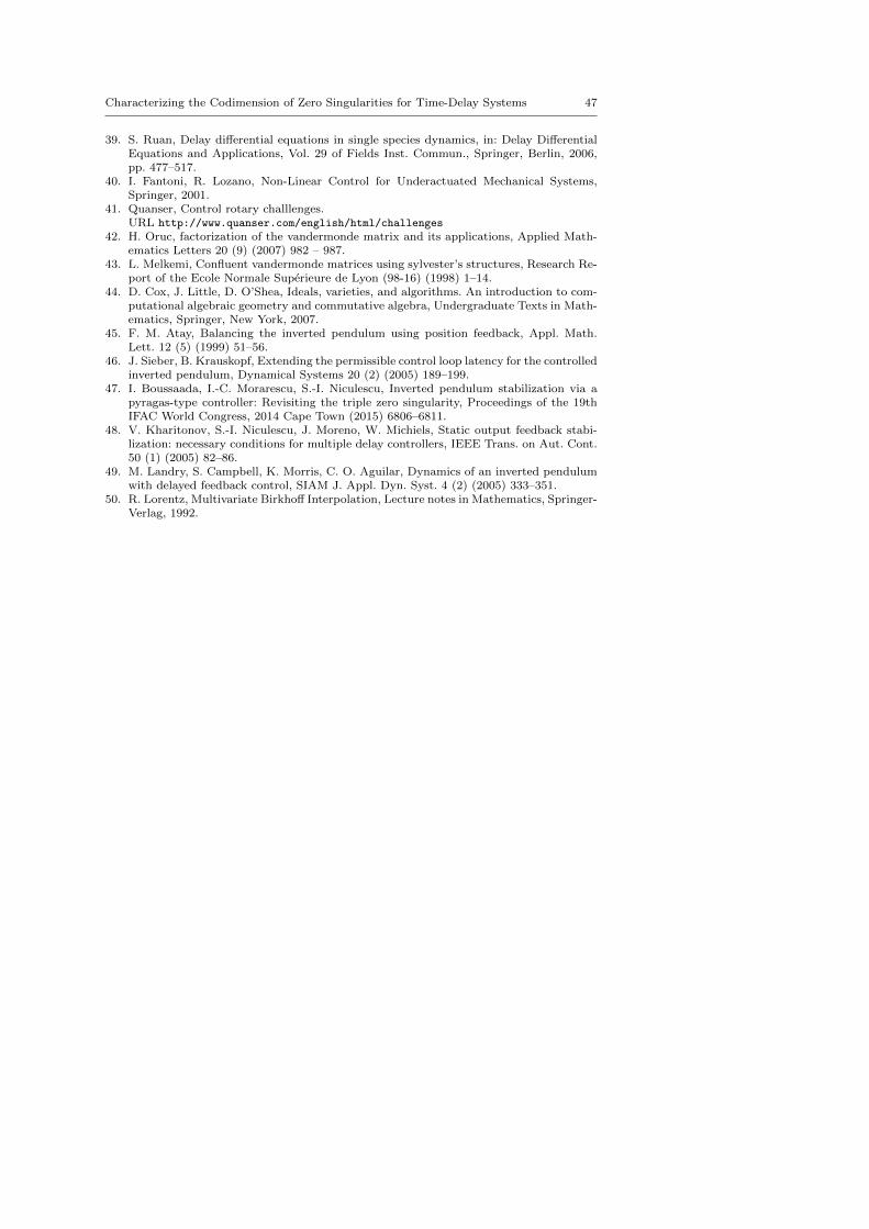
Characterizing the Codimension of Zero Singularities for Time-Delay Systems 47
39. S. Ruan, Delay differential equations in single species dynamics, in: Delay DifferentialEquations and Applications, Vol. 29 of Fields Inst. Commun., Springer, Berlin, 2006,pp. 477–517.
40. I. Fantoni, R. Lozano, Non-Linear Control for Underactuated Mechanical Systems,Springer, 2001.
41. Quanser, Control rotary challlenges.URL http://www.quanser.com/english/html/challenges
42. H. Oruc, factorization of the vandermonde matrix and its applications, Applied Math-ematics Letters 20 (9) (2007) 982 – 987.
43. L. Melkemi, Confluent vandermonde matrices using sylvester’s structures, Research Re-port of the Ecole Normale Superieure de Lyon (98-16) (1998) 1–14.
44. D. Cox, J. Little, D. O’Shea, Ideals, varieties, and algorithms. An introduction to com-putational algebraic geometry and commutative algebra, Undergraduate Texts in Math-ematics, Springer, New York, 2007.
45. F. M. Atay, Balancing the inverted pendulum using position feedback, Appl. Math.Lett. 12 (5) (1999) 51–56.
46. J. Sieber, B. Krauskopf, Extending the permissible control loop latency for the controlledinverted pendulum, Dynamical Systems 20 (2) (2005) 189–199.
47. I. Boussaada, I.-C. Morarescu, S.-I. Niculescu, Inverted pendulum stabilization via apyragas-type controller: Revisiting the triple zero singularity, Proceedings of the 19thIFAC World Congress, 2014 Cape Town (2015) 6806–6811.
48. V. Kharitonov, S.-I. Niculescu, J. Moreno, W. Michiels, Static output feedback stabi-lization: necessary conditions for multiple delay controllers, IEEE Trans. on Aut. Cont.50 (1) (2005) 82–86.
49. M. Landry, S. Campbell, K. Morris, C. O. Aguilar, Dynamics of an inverted pendulumwith delayed feedback control, SIAM J. Appl. Dyn. Syst. 4 (2) (2005) 333–351.
50. R. Lorentz, Multivariate Birkhoff Interpolation, Lecture notes in Mathematics, Springer-Verlag, 1992.

![Mean Curvature Flow in Higher Codimension: Introduction ...€¦ · Mean Curvature Flow in Higher Codimension: Introduction and Survey 233 is [28]. For the curve shortening flow](https://static.fdocuments.in/doc/165x107/5f1057b37e708231d448a30a/mean-curvature-flow-in-higher-codimension-introduction-mean-curvature-flow.jpg)