Bank of Canada staff analytical notes are short articles that focus on topical issues relevant to the current economic and financial context, produced independently from the Bank’s Governing Council. This work may support or challenge prevailing policy orthodoxy. Therefore, the views expressed in this note are solely those of the authors and may differ from official Bank of Canada views. No responsibility for them should be attributed to the Bank.

www.bank-banque-canada.ca

Staff Analytical Note/Note analytique du personnel 2018-34

Characterizing the Canadian Financial Cycle with Frequency Filtering Approaches

by Andrew Lee-Poy

Financial Stability Department Bank of Canada Ottawa, Ontario, Canada K1A 0G9 aleepoy@bankofcanada.ca

ISSN 2369-9639 © 2018 Bank of Canada

Acknowledgements

I would like to thank Jason Allen, Thibaut Duprey, Fuchun Li and Adi Mordel for very helpful comments and suggestions. I am also thankful for comments provided by participants at various brown-bag meetings.

ii

Abstract

In this note, I use two multivariate frequency filtering approaches to characterize the Canadian financial cycle by capturing fluctuations in the underlying variables with respect to a long-term trend. The first approach is a dynamically weighted composite, and the second is a stochastic cycle model. Applying the two approaches to Canada yields several findings. First, the Canadian financial cycle is more than twice as long as the business cycle, with an amplitude almost four times greater. Second, the overall Canadian financial cycle is most strongly associated with household credit and house prices. Third, while Canadian house prices are mostly associated with the financial cycle, they are also significantly tied to the business cycle. Lastly, house prices are found to lead the overall financial cycle. These results are generally in line with findings for other countries studied in literature. Additionally, I compare each approach’s proneness to revision and find that both are more reliable, when monitored in real time, than the Basel III total credit-to-GDP gap. Nonetheless, further work is encouraged to investigate more variable combinations and undertake a cross-country analysis since data on systemic financial stress in Canada are limited. It should be noted that since the approaches produce a measure of the financial cycle relative to trend, comparison with level indicators (as those monitored in the Bank of Canada’s Financial System Review) is not straightforward.

Bank topics: Business fluctuations and cycles; Financial stability; Monetary and financial indicators; Recent economic and financial developments; Econometric and statistical methods JEL codes: C01, C13, C14, C18, C32, C51, C52, E32, E66, G01, G18

Résumé

Pour décrire le cycle financier au Canada, j’emploie deux méthodes utilisant des filtres à fréquences multiples afin d’extraire les fluctuations des variables sous-jacentes par rapport à leur tendance de long terme : un indice composite à pondérations dynamiques et un modèle à tendance stochastique. Plusieurs résultats se dégagent de l’application de ces deux méthodes aux données pour le Canada. Premièrement, le cycle financier y est plus de deux fois plus long et d’une amplitude presque quatre fois plus grande que le cycle économique. Deuxièmement, le cycle financier est au Canada très étroitement lié au crédit aux ménages et aux prix des logements. Troisièmement, si les variations des prix des logements s’expliquent en grande partie par le cycle financier, elles dépendent aussi largement du cycle économique. Enfin, l’évolution des prix des logements est en avance sur l’ensemble du cycle financier. Ces résultats sont globalement conformes à ceux présentés dans la littérature pour d’autres pays. Par ailleurs, j’examine jusqu’à quel point les estimations obtenues par les deux méthodes sont sujettes à révision et observe que ces dernières sont toutes deux plus fiables, en temps réel, que l’écart crédit total / PIB prévu dans le dispositif de Bâle III. Il reste qu’il serait bon, dans des travaux futurs, de se pencher sur d’autres combinaisons de variables et d’étendre l’analyse à d’autres pays, puisqu’il existe peu de données relatives aux tensions financières systémiques au Canada. Étant donné que l’application de ces méthodes se traduit par une mesure du cycle financier par rapport à sa tendance, la comparaison avec des indicateurs « de niveau » (comme ceux dont

iii

l’évolution est rapportée dans la Revue du système financier de la Banque du Canada), ne va pas de soi.

Sujets : Cycles et fluctuations économiques; Stabilité financière; Indicateurs monétaires et financiers; Évolution économique et financière récente; Méthodes économétriques et statistiques Codes JEL : C01, C13, C14, C18, C32, C51, C52, E32, E66, G01, G18

1

1| Introduction The term “financial cycle” is used in Borio (2012) to broadly refer to interactions among financial factors that can amplify economic fluctuations and potentially lead to severe financial stress and affect the real economy. Studies to better understand the financial cycle and develop indicators to monitor its evolu-tion are important for informing countercyclical macroprudential policy, which aims to attenuate the impact of the cycle. For example, Basel III recommends using the total credit-to-GDP gap to guide the calibration of its countercyclical capital buffer (BCBS 2010).

In this study, I first characterize the financial cycle in Canada by constructing synthetic financial cycle measures. I then examine the viability of these measures as real-time indicators. Specifically, I use two multivariate frequency filtering approaches. The first is a dynamically weighted composite that makes use of the correlations among a group of real and financial indicators, inspired by Schuler, Hiebert and Peltonen (2015). The second approach is a stochastic cycle model (SCM), an econometric method that decomposes a group of variables into individual trends and common business and financial cycle compo-nents, as applied in Koopman, Lit and Lucas (2016).

While there is no consensus on how to measure a financial cycle, the recent literature suggests that us-ing multivariate frequency filtering approaches to measure the cycle is one way forward. First, the two methods used here are multivariate, capturing joint influences on the financial cycle that might be missed using univariate methods such as the Basel III total credit-to-GDP gap—a benchmark indicator of credit imbalances.1 Second, the dynamic composite can be used to assess the influence of underlying components on the overall cycle. Third, the SCM can be used to estimate aspects of the overall cycle within an econometric framework, such as the average amplitude and length.

Applying the two approaches to Canada yields a number of findings. First, the Canadian financial cycle is more than twice as long as the business cycle, with an amplitude almost four times greater. This is con-sistent with the idea that financial cycle contraction phases tend to be much more drawn out, with larger long-term impacts on economic performance. For example, Borio, Disyatat and Juselius (2013) argue that the financial cycle influences the path of potential gross domestic product (GDP). Second, the overall Canadian financial cycle is most strongly associated with household credit and house prices, whereas business credit and equity prices have relatively little bearing on the overall indicator. This is consistent with vulnerabilities highlighted in recent versions of the Bank of Canada’s Financial System Review, namely household indebtedness and housing market imbalances. Third, while Canadian house prices are mostly associated with the financial cycle, they are also significantly tied to the business cycle, supporting the notion that house prices have an impact on and are influenced by both cycles. Lastly, house prices are found to lead the overall financial cycle. These results are generally in line with findings for other countries, as studied in Drehmann, Borio and Tsatsaronis (2012); Schuler, Hiebert and Peltonen (2015); Stremmel (2015); and Koopman, Lit and Lucas (2016).

Compared with Basel III’s preferred measure of the financial cycle—the credit-to-GDP gap—I find that both the dynamic and SCM approaches produce financial cycle indicators that are more robust to revi-sions. That is, when re-estimated with new data, the indicators have less resulting change in past esti-mates. This is consistent with findings in Azevedo, Koopman and Rua (2006), who find that their multi-variate approach to extracting the business cycles has improved real-time performance relative to uni-variate approaches. Koopman, Lit and Lucas (2016) adapt this approach for financial cycles. Since these 1 Drehmann, Borio and Tsatsaronis (2011) consider the Basel III total credit-to-GDP gap to be the best single indicator of system-wide vulnera-

bilities. However, Duprey, Grieder and Hogg (2017) highlight the limitations of monitoring vulnerabilities in the Canadian context. Basel III recommends this indicator as a guide to calibrating the countercyclical buffer (BCBS 2010).

2

two multivariate approaches are less prone to revisions, they are more reliable from a policy-making perspective.

The rest of this paper is organized as follows. Section 2 reviews the literature on characterizing financial cycles through frequency filtering; Section 3 discusses the data; Section 4 covers the results; and Section 5 concludes and offers suggestions for future work.

2| Background and literature To properly estimate the financial cycle component from an economic time series, one needs to remove the trend from non-stationary data, by differentiating short- and medium-term developments from long-term characteristics. While there is no generally accepted methodology for de-trending non-sta-tionary indicators, frequency filters—such as the dynamic composite and SCM approaches—offer a way to do so.

Traditionally, frequency filtering methods have been applied to quarterly data to identify and under-stand business cycle fluctuations within a period of 1.5 to 8 years—a range that was usually considered most important for the business cycle (see Christiano and Fitzgerald 2003 and Harvey and Trimbur 2003). When measuring the financial cycles across countries, studies typically focus on periods of 8 to 30 years. This range was established in seminal work by Drehmann, Borio and Tsatsaronis (2012), who find that the most important cyclical patterns occur within this range.

One of the first applications of frequency filters in characterizing the financial cycle is found in Aikman, Haldane and Nelson (2015), where a bandpass filter proposed by Christiano and Fitzgerald (2003) is used to isolate medium- and shorter-term components from series such as total credit and GDP, respectively. Like others before (e.g., Schularick and Taylor 2012 and Jorda, Schularick and Taylor 2011), the financial cycle is thought of only in terms of excessive credit growth.

Consistent with the notion that no single indicator can capture the financial cycle, studies such as Drehmann, Borio and Tsatsaronis (2012) extend the use of frequency filters toward a multivariate ap-proach where a composite—including asset prices—is used to characterize the financial cycle. The au-thors find that the financial cycle can be most parsimoniously explained by the co-movement of house-hold credit and house prices. They find that financial cycles tend to have larger amplitudes and longer durations than business cycles. Similarly, Stremmel (2015) and Schuler, Hiebert and Peltonen (2015) make use of correlations among selected variables in constructing their composites to emphasize the importance of co-movements among key variables through the financial cycle.

The SCM is a less-explored multivariate approach that uses an econometric frequency filter to extract the gap components of the financial and business cycles that are stochastic and common across a se-lected group of variables. This approach was originally applied in business cycle analysis, such as in Azevedo, Koopman and Rua (2006), Koopman and Azevedo (2008), and Harvey and Trimbur (2008). Since then, Galati et al. (2016) and Koopman, Lit and Lucas (2016) have expanded its application to the financial cycle. This approach offers several advantages over the approaches mentioned so far. First, un-like non-parametric filters, the cycle parameters (e.g., frequency) in this approach are estimated within an econometric framework and are not user-inputted.2 Second, this approach allows us to determine how strongly each variable’s movement is associated with the financial cycle relative to the business cy-cle.

2 See Harvey (1990), Runstler (2004), and Durbin and Koopman (2012) for technical background.

3

Overall, the literature concludes that the financial cycle (i) is longer and has a larger amplitude com-pared with the business cycle, (ii) is most easily characterized by co-movements in credit and property prices, and (iii) tends to peak around episodes of banking crises. The two measures I implement in this study confirm these findings for Canada.

3| Data Following Drehmann, Borio and Tsatsaronis (2012), I select variables with a long time series, as financial cycles tend to be longer. In Canada, time series length is restricted by house prices, for which the long-est available series starts in 1981.

The literature indicates that variable selection for constructing financial cycle indicators tends to be par-simonious and always includes total credit and residential house prices, since their interaction is consid-ered most closely related to the financial cycle. This is also consistent with the notion that financial cycle risks are associated with the increase in leverage and the potential for severe adjustments in asset prices.

For the dynamic composite, I use a set of four variables that Schuler, Hiebert and Peltonen (2015) had previously indicated as being most related to the financial cycle: household credit growth, business credit growth, house price growth and equity price growth. I use household credit and business credit as separate inputs (rather than total credit alone) because it allows for a more informative breakdown of the composite.

The variables collected for the SCM are in levels and follow Koopman, Lit and Lucas (2016): GDP, total credit, total credit-to-GDP, total credit-to-disposable income, and residential house prices.3 GDP enters the model as a proxy for the business cycle, whereas the other four indicators are meant to capture the financial cycle. Appendix 1 provides further details on the data series used.

4| Results In this section I first estimate the Canadian financial cycle using the dynamic composite and SCM ap-proaches. I then compare their performance relative to the Basel III total credit-to-GDP gap. I provide technical details on the methodologies in Appendix 2.

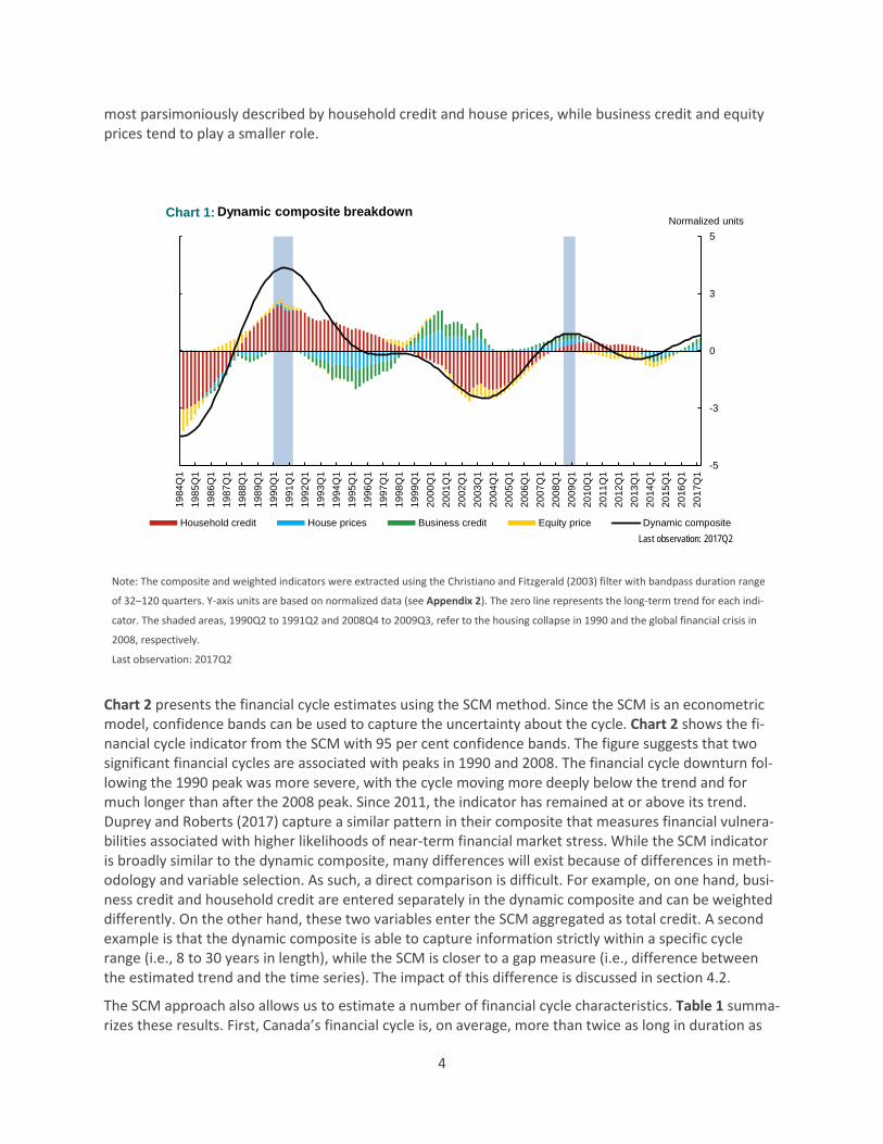
4.1| Characteristics of the Canadian financial cycle Chart 1 shows the results from the financial cycle estimation using the dynamic composite. One of its advantages is that the financial cycle can be broken down into its underlying components, allowing us to decompose the relative contribution of each sector. The stacked bars represent the contribution of each of the underlying indicators into the overall composite (black line). The shaded areas mark stress periods following the housing collapse in 1990 and the global financial crisis in 2008, respectively. The 1990s cy-cle is much larger than the 2008 cycle because of a much larger buildup of imbalances detected in the housing market and household sectors. More specifically, the higher contribution of these variables within the composite is the result of (i) house prices and household credit rising above their long-term trends for several years leading up to the 1990 collapse, and (ii) their high correlation during that period, which garners a higher weighting. While household credit grew quickly leading up to 2008, the level did not greatly exceed its long-term trend when the global financial crisis materialized, nor was there as large a buildup of housing market imbalances. Overall, Chart 1 shows that Canada’s financial cycle is

3 I follow Koopman, Lit and Lucas (2016) in focusing on total-credit-based indicators when estimating the financial cycle with the SCM to facili-

tate the identification of the overall cycle. The model fails to converge when using the same indicators as the dynamic composite approach.

4

most parsimoniously described by household credit and house prices, while business credit and equity prices tend to play a smaller role.

Note: The composite and weighted indicators were extracted using the Christiano and Fitzgerald (2003) filter with bandpass duration range

of 32–120 quarters. Y-axis units are based on normalized data (see Appendix 2). The zero line represents the long-term trend for each indi-

cator. The shaded areas, 1990Q2 to 1991Q2 and 2008Q4 to 2009Q3, refer to the housing collapse in 1990 and the global financial crisis in

2008, respectively.

Last observation: 2017Q2

Chart 2 presents the financial cycle estimates using the SCM method. Since the SCM is an econometric model, confidence bands can be used to capture the uncertainty about the cycle. Chart 2 shows the fi-nancial cycle indicator from the SCM with 95 per cent confidence bands. The figure suggests that two significant financial cycles are associated with peaks in 1990 and 2008. The financial cycle downturn fol-lowing the 1990 peak was more severe, with the cycle moving more deeply below the trend and for much longer than after the 2008 peak. Since 2011, the indicator has remained at or above its trend. Duprey and Roberts (2017) capture a similar pattern in their composite that measures financial vulnera-bilities associated with higher likelihoods of near-term financial market stress. While the SCM indicator is broadly similar to the dynamic composite, many differences will exist because of differences in meth-odology and variable selection. As such, a direct comparison is difficult. For example, on one hand, busi-ness credit and household credit are entered separately in the dynamic composite and can be weighted differently. On the other hand, these two variables enter the SCM aggregated as total credit. A second example is that the dynamic composite is able to capture information strictly within a specific cycle range (i.e., 8 to 30 years in length), while the SCM is closer to a gap measure (i.e., difference between the estimated trend and the time series). The impact of this difference is discussed in section 4.2.

The SCM approach also allows us to estimate a number of financial cycle characteristics. Table 1 summa-rizes these results. First, Canada’s financial cycle is, on average, more than twice as long in duration as

-5

-3

0

3

5

1984

Q1

1985

Q1

1986

Q1

1987

Q1

1988

Q1

1989

Q1

1990

Q1

1991

Q1

1992

Q1

1993

Q1

1994

Q1

1995

Q1

1996

Q1

1997

Q1

1998

Q1

1999

Q1

2000

Q1

2001

Q1

2002

Q1

2003

Q1

2004

Q1

2005

Q1

2006

Q1

2007

Q1

2008

Q1

2009

Q1

2010

Q1

2011

Q1

2012

Q1

2013

Q1

2014

Q1

2015

Q1

2016

Q1

2017

Q1

Normalized units

Household credit House prices Business credit Equity price Dynamic composite

Chart 1: Dynamic composite breakdown

Last observation: 2017Q2

5

the business cycle and almost four times larger in amplitude (standard deviation), which is consistent with evidence from other cross-country studies (Drehmann, Borio and Tsatsaronis 2012 and Koopman, Lit and Lucas 2016). This suggests the relative danger of the financial cycle, since large upswings tend to be followed by large downturns and are closely associated with financial crises, which can have a signifi-cant impact on longer-term economic performance (Drehmann, Borio and Tsatsaronis 2012 and Borio 2013). Second, the bottom portion of Table 1 shows the relative association of each input variable rela-tive to the estimated financial or business cycles. While credit-based indicators are almost completely tied to the financial cycle, house prices have a relatively stronger association to the business cycle. Koopman, Lit and Lucas (2016) also find a relatively strong relationship between house prices and the business cycle in other developed countries, supporting the notion that house prices have an impact on and are influenced by both cycles. For example, an upswing in house prices can influence the business cycle by incentivizing more residential investment and the financial cycle through increased borrowing capacity. At the same time, an upswing in house prices can be driven by the business cycle through higher wages, and by the financial cycle through looser lending conditions. Lastly, the model estimates that house prices lead the overall financial cycle by about six quarters, on average. For a visual compari-son of the estimated financial and business cycles under both the SCM and dynamic composite ap-proaches, see Chart 3.

Note: The zero line represents the long-term trend. The SCM indicator is estimated via a Kalman smoother. The shaded areas, 1990Q2 to

1991Q2 and 2008Q4 to 2009Q3, refer to the housing collapse in 1990 and the global financial crisis in 2008, respectively.

Last observation: 2017Q2

-25-20-15-10-50510152025

1984

Q1

1985

Q1

1986

Q1

1987

Q1

1988

Q1

1989

Q1

1990

Q1

1991

Q1

1992

Q1

1993

Q1

1994

Q1

1995

Q1

1996

Q1

1997

Q1

1998

Q1

1999

Q1

2000

Q1

2001

Q1

2002

Q1

2003

Q1

2004

Q1

2005

Q1

2006

Q1

2007

Q1

2008

Q1

2009

Q1

2010

Q1

2011

Q1

2012

Q1

2013

Q1

2014

Q1

2015

Q1

2016

Q1

2017

Q1

% deviation from trend

95% confidence bands SCM financial cycle indicator

Chart 2: Stochastic cycle indicator

Last observation: 2017Q2

6

Table 1: Stochastic cycle model results

Business cycle Financial cycle

Cycle length (years) 4.08 10.25 Relative amplitude 1.00 3.94

Cycle contributions GDP 100% 0%

Total credit 1% 99% Total credit-to-GDP 17% 83%

Total credit-to-disposable income 1% 99%

Average house price 34% 66%

Notes: Percentages explain how much of a variable’s variation is explained by the business and financial cycles. Relative amplitude for the

financial cycle is measured as the ratio of the standard deviation of the financial cycle component divided by the standard deviation of the

business cycle component. Identification restrictions imply that cyclicality in GDP is explained entirely by the business cycle component.

Chart 3: Financial and business cycle durations

a. Stochastic cycle indicator

b. Dynamic composite

Note: The business cycle indicators are estimated output gaps consistent with each filtering approach. In panel b, a smoothed output gap is

estimated using the Christiano-Fitzgerald filter (tuned to a range of 6 to 32 quarters) on GDP deflated by total CPI. In panel a, the gap is esti-

mated via within the SCM and is identified using GDP deflated by total CPI. The zero line represents the long-term trend for each indicator.

The shaded areas, 1990Q2 to 1991Q2 and 2008Q4 to 2009Q3, refer to the housing collapse in 1990 and the global financial crisis in 2008,

respectively.

Last observation: 2017Q2

-20

-15

-10

-5

0

5

10

15

20

25

% deviation from trend

Business cycle indicator 95% confidence bandsFinancial cycle indicator

Last observation: 2017Q2

-4

-3

-2

-1

0

1

2

3

4

Normalized units

Business cycle indicator Financial cycle indicator

Last observation: Q2 2017

7

4.2| Comparing indicators Borio (2013), Drehmann, Borio and Tsatsaronis (2011) and Drehmann and Tsatsaronis (2014) consider the total credit-to-GDP gap as the best single indicator of the financial cycle. In this section, I compare it with the multivariate approaches in this study.

The estimates of the financial cycle of the three approaches are plotted in Chart 4. We can observe that both the SCM indicator and the total credit-to-GDP gap are less smooth relative to the dynamic compo-site. This makes sense, because the SCM indicator is similar to a gap measure (i.e., high-pass filter), which the total credit-to-GDP Hodrick-Prescott (HP) gap precisely is. The implication is that while the long-term trend is filtered out, both medium- and short-term developments are captured in the cycle component. The dynamic composite, on the other hand, relies on bandpass filtering, allowing it to focus only on the medium term, resulting in a smoother indicator that does not react to short-term shocks.4

A key weakness of the total credit-to-GDP gap is that it suffers from over-reliance on a single indicator that depends crucially on GDP, reacting to macroeconomic shocks and other business cycle fluctuations. This dependence on GDP and the fact that it is a gap measure emphasizes shorter-term macroeconomic shocks, reducing the effectiveness of the total credit-to-GDP gap as an indicator of medium-term imbal-ances. For instance, a negative macroeconomic shock results in a dip in GDP growth, causing a tempo-rary jump in the overall indicator.5 We can observe such a jump in 2008 and 2014, similar to the finan-cial stress indicator in Duprey (forthcoming). In contrast, while the SCM indicator considers the total credit-to-GDP ratio, its multivariate and econometric approach mitigates the weakness of that single in-dicator.6 And like the dynamic composite, it captures the rise in financial imbalances leading into the 1990s housing price crash and the 2008 global financial crisis, when using all available data. The total credit-to-GDP gap misses both events.

4.3| Real-time performance An indicator that is reliable in real time should not experience revision over time. In this section, I assess and compare the real-time performance of the multivariate approaches in this study with the Basel III total credit-to-GDP gap.

A key challenge with indicators that use frequency filters is that past estimates can be revised when re-estimated in subsequent periods, leading to increased uncertainty and inaction bias when monitoring them in real time. As a solution to this “end-point problem,” Drehmann and Tsatsaronis (2014) suggest using a one-sided version of the frequency filter.7 Since this is a historical series, it does not revise. However, this practice does not serve to improve the indicator, since it merely side-steps revisions by ignoring information contained in data from later periods. In fact, Edge and Meisenzahl (2011) show that revisions are almost entirely tied to past estimates being updated once new data become available. Fur-thermore, they find that revisions in the total credit-to-GDP gap can sometimes be as large as the gap itself.

4 See Appendix 3 for a brief background on frequency filtering.

5 A more detailed discussion on the effect of macroeconomic shocks on the total credit-to-GDP gap (and other similar measures) can be found in Duprey, Grieder and Hogg (2017).

6 In fact, estimating the SCM without total credit-to-GDP or total credit-to-disposable income, yields a very similar financial cycle indicator.

7 A one-sided indicator is a historical series of end points resulting from recursively re-estimating the indicator each period t, using only data up to t.

8

Following Edge and Meisenzahl (2011) and Azevedo, Koopman and Rua (2006), I assess real-time perfor-mance by comparing each indicator, estimated using the full sample, against its one-sided counterparts. For each indicator, three comparative measures are computed: correlation, sign concordance and sig-nal-to-noise ratio. Correlation is a simple measure of contemporaneous directional alignment between the one-sided and full-sample indicators, where a coefficient closer to 1 is better. Sign concordance is the proportion of time where the sign of the one-sided indicator matches that of the indicator estimated using the full sample, where a ratio closer to 1 is better. The signal-to-noise ratio here is measured as 1 minus the standard deviation of revisions relative to the standard deviation of the indicator estimated with the full sample, where a value closer to 1 is better. Chart 5 provides a visual comparison and Table 2 summarizes the results. The metrics show that, while multivariate approaches in this study are still subject to revisions, they outperform the total credit-to-GDP gap as real-time indicators and there-fore are considered more reliable from a policy-making perspective. Correlation, sign concordance and signal-to-noise are much closer to unity. This is consistent with Azevedo, Koopman and Rua (2006), who similarly find that a multivariate stochastic cycle model approach outperforms other univariate ap-proaches, using the same metrics.

Chart 5: Visual comparison of one-sided versus full-sample indicators

a. Dynamic composite

b. Stochastic cycle model

c. Total credit-to-GDP gap

Full sample Real time

Note: The y-axis for panel a is in normalized units, while panel b and panel c are deviations from trend, as a percent of GDP. The zero line

represents the long-term trend for each indicator. For the SCM: the model is estimated using data up to 2003, at which point the Kalman

filter estimates subsequent periods using the same parameters. The shaded areas, 1990Q2 to 1991Q2 and 2008Q4 to 2009Q3, refer to the

housing collapse in 1990 and the global financial crisis in 2008, respectively.

Last observation: 2017Q2

-4

-3

-2

-1

0

1

2

3

4

1984

Q1

1986

Q1

1988

Q1

1990

Q1

1992

Q1

1994

Q1

1996

Q1

1998

Q1

2000

Q1

2002

Q1

2004

Q1

2006

Q1

2008

Q1

2010

Q1

2012

Q1

2014

Q1

2016

Q1

Last observation: 2017Q2

Normalized units

-20

-15

-10

-5

0

5

10

15

20

1984

Q1

1986

Q1

1988

Q1

1990

Q1

1992

Q1

1994

Q1

1996

Q1

1998

Q1

2000

Q1

2002

Q1

2004

Q1

2006

Q1

2008

Q1

2010

Q1

2012

Q1

2014

Q1

2016

Q1

Last observation: 2017Q2

% deviation from trend

-10

-5

0

5

10

15

20

1984

Q1

1986

Q1

1988

Q1

1990

Q1

1992

Q1

1994

Q1

1996

Q1

1998

Q1

2000

Q1

2002

Q1

2004

Q1

2006

Q1

2008

Q1

2010

Q1

2012

Q1

2014

Q1

2016

Q1

Last observation: 2017Q2

% deviation from trend

9

Table 2: Measures of real-time reliability

Measure Measurement period Correlation Sign

concordance Signal-to-noise

Credit-to-GDP gap (HP filter) Up to 2011Q2 0.50 0.61 0.00

Dynamic composite Up to 2011Q2 0.75 0.83 0.32

Stochastic cycle model 2005Q3 to 2011Q2 0.99 0.71 0.83

Note: Worst scores are highlighted in red and best scores are highlighted in green. The signal-to-noise ratio is computed as 1 minus the

standard deviation of the revisions divided by the standard deviation of the full-sample measure. Details on the measurement periods can

be found in Appendix 2.

5| Conclusion Studies that aim to better understand the financial cycle and develop indicators to monitor its evolution are important for developing and informing countercyclical macroprudential policy and, in particular, Basel III’s countercyclical capital buffer, as it targets the financial cycle. The approaches in this study pro-vide multivariate ways of using historical data to interpret macrofinancial variables relative to a bench-mark. Specifically, they identify and help characterize financial cycle patterns and are more robust to re-visions relative to univariate approaches.

There are four key findings regarding the characteristics of the Canadian financial cycle. First, the aver-age financial cycle in Canada is estimated to be more than twice as long as the average business cycle, with an amplitude almost four times greater. This suggests the relative danger of the financial cycle since large upswings tend to be followed by large downturns and are closely associated with financial crises, which can have a significant impact on long-term economic performance. Second, I find that the Canadian financial cycle is most strongly associated with household credit and house prices. In contrast, business credit and equity prices have relatively little bearing on the overall indicator. Third, while Cana-dian house prices are mostly associated with the financial cycle, they are also significantly tied to the business cycle, supporting the notion that house prices have an impact on and are influenced by both cycles. Last, house prices are found to lead the overall financial cycle.

Multiple measures of reliability suggest that the multivariate approaches in this study still experience revision as new data become available, but are more robust than the Basel III total credit-to-GDP gap, making them relatively more viable as regularly monitored indicators.

A key limitation of the approaches in this study, and statistical filters in general, is that they are suscepti-ble to the “level effect,” where persistent and excessive growth can be erroneously incorporated into the estimated long-term trend. This can, at times, result in signals that underestimate the level of credit-related imbalances in the financial system. Furthermore, the level effect is difficult to measure. Since frequency filters are designed to estimate a long-term trend subject to the remaining cycle component being stationary, this implies that the level effect is caused by persistently high growth relative to the length of data available.

10

While there is no generally accepted method for measuring financial cycles, the approaches in this study offer a methodology to extract such a measure from economic data series. However, future work is en-couraged for three reasons. First, while the variable selection in this study is more or less prescribed by existing literature, more variable combinations should also be investigated. One example is to include a global aspect of financial imbalance in the Canadian measure. Second, we need to better understand the “level effect.” Comparing real-time estimates with outcomes of financial events (both economic and pol-icy response) through history can be a starting point, since it serves as a back-test to determine whether the approaches in this study capture a level of vulnerabilities that is commensurate to would-be out-comes. A cross-country analysis can contribute here, as systemic financial stress data in Canada (and likely most individual advanced economies) are limited. And last, since the approaches produce a meas-ure of the financial cycle relative to trend, comparison with level indicators (as those monitored in the Bank of Canada’s Financial System Review) might not be straightforward.

11

References Aikman, D., A. G. Haldane and B. D. Nelson. 2015. “Curbing the Credit Cycle.” The Economic Journal 125 (585): 1072–1109.

Azevedo, J. V. E., S. J. Koopman and A. Rua. 2006. “Tracking the Business Cycle of the Euro Area: A Multi-variate Model-Based Bandpass Filter.” Journal of Business & Economic Statistics 24 (3): 278–290.

Basel Committee on Banking Supervision (BCBS). 2010. “Guidance for National Authorities Operating the Countercyclical Capital Buffer.” Bank for International Settlements.

Borio, C. 2012. “The Financial Cycle and Macroeconomics: What Have we Learnt?” Bank for International Settlements Working Paper No. 395.

Borio, C. 2013. “Macroprudential Policy and the Financial Cycle: Some Stylised Facts and Policy Sugges-tions.” Presentation at the International Monetary Fund conference, Rethinking Macro Policy II: First Steps and Early Lessons Conference, Washington, DC, April 16–17.

Borio, C., P. Disyatat and M. Juselius. 2013. “Rethinking Potential Output: Embedding Information about the Financial Cycle.” Bank for International Settlements Working Paper No. 404.

Christiano, L. J. and T. J. Fitzgerald. 2003. “The Band Pass Filter.” International Economic Review 44 (2): 435–465.

Drehmann, M., C. Borio and K. Tsatsaronis. 2011. “Anchoring Countercyclical Capital Buffers: The Role of Credit Aggregates.” Bank for International Settlements Working Paper No. 355.

Drehmann, M., C. Borio and K. Tsatsaronis. 2012. “Characterising the Financial Cycle: Don’t Lose Sight of the Medium Term!” Bank for International Settlements Working Paper No. 380.

Drehmann, M. and K. Tsatsaronis. 2014. “The Credit-to-GDP Gap and Countercyclical Capital Buffers: Questions and Answers.” Bank for International Settlements Quarterly Review, March.

Duprey, T. Forthcoming. “Canadian Financial Stress and Macroeconomic Conditions.” Bank of Canada Staff Working Paper.

Duprey, T. and T. Roberts. 2017. “A Barometer of Canadian Financial System Vulnerabilities.” Bank of Canada Staff Analytical Note No. 2017-24.

Duprey, T., T. Grieder and D. Hogg. 2017. “Recent Evolution of Canada’s Credit-to-GDP Gap: Measure-ment and Interpretation.” Bank of Canada Staff Analytical Note No. 2017-25.

Durbin, J. and S. J. Koopman. 2012. Time Series Analysis by State Space Methods. 2nd edition. Oxford Uni-versity Press.

Edge, R. M. and R. R. Meisenzahl. 2011. “The Unreliability of Credit-to-GDP Ratio Gaps in Real-Time: Im-plications for Countercyclical Capital Buffers.” Board of Governors of the Federal Reserve System, Fi-nance and Economics Discussion Series Working Paper No. 2011-37.

Galati, G., I. Hindrayanto, S. J. Koopman and M. Vlekke. 2016. “Measuring Financial Cycles in a Model-Based Analysis: Empirical Evidence for the United States and the Euro Area.” Economics Letters 145 (C): 83–87.

Harvey, A. 1990. Forecasting, Structural Time Series Models and the Kalman Filter. Cambridge: Cam-bridge University Press.

12

Harvey, A. C. and T. M. Trimbur. 2003. “General Model-based Filters for Extracting Cycles and Trends in Economic Time Series.” The Review of Economics and Statistics 85 (2): 244–255.

Harvey, A. and T. Trimbur. 2008. “Trend Estimation and the Hodrick-Prescott Filter.” Journal of the Japa-nese Statistical Society (volume in honour of H. Akaike) 38 (1): 41–49.

Hodrick, R. T. and E. C. Prescott. 1997. “Postwar U.S. Business Cycles: An Emprical Investigation.” Journal of Money, Credit and Banking 29 (1):1–16.

Hollo, D., M. Kremer and M. Lo Duca. 2012. “CISS—A Composite Indicator of Systemic Stress in the Fi-nancial System.” European Central Bank Working Paper No. 1426.

Jordà, O., M. Schularick and A. M. Taylor. 2011. “Financial Crises, Credit Booms, and External Imbal-ances: 140 Years of Lessons,” IMF Economic Review 59 (2): 340–378.

Kalman, R. E. 1960. “A New Approach to Linear Filtering and Prediction Problems.” Journal of Basic Engi-neering 82 (1, Series D): 35–45.

Koopman, S. J. and J. V. Azevedo. 2008. “Measuring Synchronization and Convergence of Business Cycles for the Euro area, UK and US” Oxford Bulletin of Economics and Statistics, 2008, vol. 70, issue 1, 23-51.

Koopman, S. J., R. Lit and A. Lucas. 2016. “Model-based Business Cycle and Financial Cycle Decomposi-tion for Europe and the U.S.” Tinbergen Institute Discussion Paper No. 16-051/IV.

Runstler, G. 2004. “Modelling Phase Shifts Among Stochastic Cycles.” The Econometrics Journal 7 (1): 232–248.

Schularick, M. and A. M. Taylor. 2012. “Credit Booms Gone Bust: Monetary Policy, Leverage Cycles, and Financial Crises, 1870-2008,” American Economic Review 102 (2): 1029–1061.

Schuler, Y. S., P. P. Hiebert and T. A. Peltonen. 2015. “Characterising the Financial Cycle: A Multivariate and Time-Varying Approach.” European Central Bank Working Paper No. 1846.

Stremmel, H. 2015. “Capturing the Financial Cycle in Europe.” European Central Bank Working Paper No. 1811.

13

Appendix 1| Data sources

Total credit = Household credit + Business credit

Household credit – source: CANSIM

• = Consumer credit (v122707) + Mortgage credit (v122738)

Business credit – source: CANSIM

• = Business credit, including equity and warrants, and trust units (v122643) – Equity and warrants (v122642) – Trust units (v20638380)

Nominal gross domestic product (GDP) – source: CANSIM (v62305783)

Nominal disposable income – source: CANSIM (v62305981)

Total consumer price index (CPI) – source: CANSIM (v41690973)

Equity prices (TSX Index) – source: CANSIM (v122620)

Average house price – source: Canadian Real Estate Association (CREA) – Multiple Listing Service (MLS)

Table A-1: Summary statistics

Year-over-year percentage growth

Indexed level (2017Q2 value =

100)

Mean StDev

Avg. 5-year growth lead-ing to 1990

peak

Avg. 5-year growth lead-ing to 2008

peak Last value (2017Q2)

Value at 1990 peak

Value at 2008 peak

Total credit 3.9% 3.0% 7.0% 6.2% 4.6% 0.35 0.70

Household credit 4.7% 3.9% 9.0% 8.2% 4.4% 0.28 0.71

Business credit 3.0% 4.4% 5.2% 3.4% 4.9% 0.46 0.68

Equity prices 2.8% 18.3% 3.7% 11.3% 6.3% 0.39 0.87

Average house price 2.5% 6.7% 8.3% 6.5% 0.2% 0.46 0.67 The data set is quarterly and spans from 1981Q1 to 2017Q2. Variables are deflated by total CPI.

14

Appendix 2| Methodology

A2.1| Transforming and normalizing data All nominal macro variables are deflated by the total consumer price index (CPI) and logged. Ratios do not receive this transformation.

For the composite, differencing is done on a year-over-year (yoy) basis and the data are normalized so that they are unit-less and comparable—a necessary step for aggregation. Let x represent an input varia-ble as a raw time series and let y represent its normalization. The normalization procedure is as follows:

𝑦𝑦 = 𝑥𝑥−𝑥𝑥5%𝑥𝑥95%−𝑥𝑥5%

(1.1)

Each series is feature-scaled by its 5th and 95th percentiles. When periodically recalculating indicators that use standardized data, it is important that the scale remain relatively constant over time to main-tain comparability.8 This practice essentially mitigates the next outlier from influencing the scale of the data when incorporating new data from one period to the next (versus using maximums and mini-mums). Since the outliers are not actually being modified, the results are not affected.

Unlike a composite, the SCM approach does not require normalization of data and the input variables simply enter as a log level or ratio.

A2.2| Dynamically weighted composite Inspired from work by Schuler, Hiebert and Peltonen (2015) and Drehmann, Borio and Tsatsaronis (2012), this approach applies the Christiano-Fitzgerald (CF) filter to a dynamically weighted composite to isolate medium-term fluctuations.

Let 𝑌𝑌𝑡𝑡 = �𝑦𝑦1,𝑡𝑡 , … ,𝑦𝑦𝑀𝑀,𝑡𝑡� where M is the number of input variables and each time series 𝑦𝑦𝑖𝑖,𝑡𝑡 is normal-ized. The composite is a weighted sum of the underlying indicators. Each indicator’s weight is deter-mined by the sum of its correlations with every other input variable. It is formulated as follows:

𝐶𝐶𝐶𝐶𝐶𝐶𝐶𝐶𝐶𝐶𝐶𝐶𝐶𝐶𝐶𝐶𝐶𝐶𝑡𝑡 = 1𝜄𝜄′𝐶𝐶𝑡𝑡𝜄𝜄

∙ 𝜄𝜄′𝐶𝐶𝑡𝑡𝑌𝑌𝑡𝑡, (2.1)

where 𝐶𝐶𝑡𝑡 is a matrix of time-varying pairwise correlations among the input variables. 𝜄𝜄 is a vector of ones. The numerator and denominator are scalars.

𝐶𝐶𝑡𝑡 = �𝑐𝑐𝐶𝐶𝑐𝑐𝑐𝑐11,𝑡𝑡 ⋯ 𝑐𝑐𝐶𝐶𝑐𝑐𝑐𝑐1𝑀𝑀,𝑡𝑡

⋮ ⋱ ⋮𝑐𝑐𝐶𝐶𝑐𝑐𝑐𝑐𝑀𝑀1,𝑡𝑡 ⋯ 𝑐𝑐𝐶𝐶𝑐𝑐𝑐𝑐𝑀𝑀𝑀𝑀,𝑡𝑡

� (2.2)

𝑐𝑐𝐶𝐶𝑐𝑐𝑐𝑐𝑖𝑖𝑖𝑖,𝑡𝑡 = 𝜎𝜎𝑖𝑖𝑖𝑖,𝑡𝑡 ��𝜎𝜎𝑖𝑖𝑖𝑖,𝑡𝑡𝜎𝜎𝑖𝑖𝑖𝑖,𝑡𝑡�⁄ (2.3)

𝜎𝜎𝑖𝑖𝑖𝑖,𝑡𝑡 = 𝜆𝜆𝜎𝜎𝑖𝑖𝑖𝑖,𝑡𝑡−1 + (1 − 𝜆𝜆)�𝑦𝑦𝑖𝑖,𝑡𝑡 − 𝑦𝑦𝑖𝑖,𝑡𝑡𝑀𝑀𝑀𝑀10��𝑦𝑦𝑖𝑖,𝑡𝑡 − 𝑦𝑦𝑖𝑖,𝑡𝑡𝑀𝑀𝑀𝑀10� (2.4)

8 The [5, 95] percentiles seem to work well, while there is a significant jump in proneness to rescaling when switching to the [2.5, 97.5] percen-

tiles.

15

Lambda is a decay factor set to 0.89 as in Schuler, Hiebert and Peltonen (2015).9 �𝑦𝑦𝑖𝑖,𝑡𝑡 − 𝑦𝑦𝑖𝑖,𝑡𝑡𝑀𝑀𝑀𝑀10� is the deviation from a 10-year moving average to capture variables moving in the same direction while limit-ing influence from the distant past.10 Schuler, Hiebert and Peltonen (2015) note that covariance initiali-zation requires about eight quarters.

To further emphasize the importance of co-movements in this approach, I set the diagonal elements of 𝐶𝐶𝑡𝑡 to zero. A key variable that has no co-movement with any other variable will have zero weight and will not be viewed as a systemic concern.

Next, the “growth” cycle is cumulated into a “level” cycle as in Drehmann, Borio and Tsatsaronis (2012) and centred on the mean (of the cumulated series) to arrive at the synthetic financial cycle indicator.11

𝐹𝐹𝐶𝐶𝑡𝑡 = ∑ 𝑓𝑓𝐶𝐶𝑓𝑓𝐶𝐶𝐶𝐶𝑐𝑐(𝐶𝐶𝐶𝐶𝐶𝐶𝐶𝐶𝐶𝐶𝐶𝐶𝐶𝐶𝐶𝐶𝐶𝐶|1𝑇𝑇)𝑡𝑡1 − 1

𝑇𝑇∑ ∑ 𝑓𝑓𝐶𝐶𝑓𝑓𝐶𝐶𝐶𝐶𝑐𝑐(𝐶𝐶𝐶𝐶𝐶𝐶𝐶𝐶𝐶𝐶𝐶𝐶𝐶𝐶𝐶𝐶𝐶𝐶|1𝑇𝑇)𝑇𝑇

1𝑇𝑇1 (2.5)

A2.3| Stochastic cycle model indicator Inspired by Koopman, Lit and Lucas (2016), this is an approach that leverages the unobserved compo-nents model framework to decompose a group of selected variables into their respective trends, and common business cycle and financial cycle components. The latter is used as an indicator.

Suppose we have a linear Gaussian state space model with a measurement equation

𝒀𝒀𝑡𝑡 = 𝒁𝒁𝜶𝜶𝑡𝑡 + 𝜺𝜺𝑡𝑡 , 𝜺𝜺𝑡𝑡 ∼ 𝑁𝑁(𝟎𝟎,𝑯𝑯) (3.1)

and transition equation

𝜶𝜶𝑡𝑡+1 = 𝑻𝑻𝜶𝜶𝑡𝑡 + 𝜼𝜼𝑡𝑡, 𝜼𝜼𝑡𝑡 ∼ 𝑁𝑁(𝟎𝟎,𝑸𝑸). (3.2)

Bold lettering represents vectors or matrices. The state vector 𝜶𝜶𝑡𝑡 contains the unobserved compo-nents we are interested in.12

𝜶𝜶𝑡𝑡 = �𝜇𝜇1𝑡𝑡 𝜈𝜈1𝑡𝑡 … 𝜇𝜇𝑀𝑀𝑡𝑡 𝜈𝜈𝑀𝑀𝑡𝑡 𝜓𝜓𝐵𝐵𝐶𝐶,𝑡𝑡 𝜓𝜓𝐵𝐵𝐶𝐶,𝑡𝑡∗ 𝜓𝜓𝐹𝐹𝐶𝐶,𝑡𝑡 𝜓𝜓𝐹𝐹𝐶𝐶,𝑡𝑡

∗ �′ ,

where 𝜇𝜇𝑖𝑖𝑡𝑡 and 𝜈𝜈𝑖𝑖𝑡𝑡 represent the trend component, 𝜓𝜓𝜅𝜅,𝑡𝑡 and 𝜓𝜓𝜅𝜅,𝑡𝑡∗ represent the cycle component

for 𝜅𝜅 ∈ {𝐵𝐵𝐶𝐶,𝐹𝐹𝐶𝐶}, and 𝛾𝛾𝜅𝜅,𝑖𝑖 is the phase shift associated with variable i. 𝜓𝜓𝜅𝜅,𝑡𝑡∗ is the “out-of-phase” por-

tion of the cycle—while we are not interested in it, it is necessary for the model. Modelling phase shifts takes into account that the cycle phases of individual variables are unlikely to have the exact same tim-ing.

The key idea in this approach is that the unobserved components are related through 𝒁𝒁 to the ob-served variables and that these components transition from one period to another according to 𝑻𝑻.

Breaking down the measurement equation

𝑦𝑦𝑖𝑖𝑡𝑡 = 𝜇𝜇𝑖𝑖𝑡𝑡 + 𝛿𝛿𝑖𝑖𝜓𝜓𝐵𝐵𝐶𝐶,𝑖𝑖𝑡𝑡 + 𝛽𝛽𝑖𝑖𝜓𝜓𝐹𝐹𝐶𝐶,𝑖𝑖𝑡𝑡 + 𝜀𝜀𝑖𝑖𝑡𝑡 , 𝜀𝜀𝑖𝑖,𝑡𝑡 ∼ 𝐶𝐶𝐶𝐶𝑖𝑖 𝑁𝑁�0,𝜎𝜎𝜀𝜀,𝑖𝑖2 � (3.3)

9 Schuler, Hiebert and Peltonen (2015) derive their approach from Hollo, Kremer and Lo Duca (2012), who use an IGARCH model to arrive at a

decay factor of 0.93 given daily data. Schuler, Hiebert and Peltonen (2015) opt for a slightly lower factor of 0.89 to account for quarterly data (fewer observations) and so initial conditions would become negligible at a faster rate.

10 The results do not seem to change significantly whether a 10-year moving average or an accumulating historical average is used.

11 Cumulating is not an issue since the cumulative of a stationary series is also stationary.

12 See Koopman, Lit and Lucas (2016) for more details.

16

𝜓𝜓𝜅𝜅,𝑖𝑖𝑡𝑡 = cos�𝛾𝛾𝜅𝜅,𝑖𝑖𝜆𝜆𝜅𝜅�𝜓𝜓𝜅𝜅,𝑡𝑡 + sin�𝛾𝛾𝜅𝜅,𝑖𝑖𝜆𝜆𝜅𝜅�𝜓𝜓𝜅𝜅,𝑡𝑡∗ , 𝜅𝜅 ∈ {𝐵𝐵𝐶𝐶,𝐹𝐹𝐶𝐶} (3.4)

Equation 3.3 shows the series of each variable i broken down into its trend and cycle components. In equation 3.4, the cycle component for each variable, 𝜓𝜓𝜅𝜅,𝑖𝑖𝑡𝑡, (whether business or financial) is a function of one common cycle. 𝛿𝛿𝑖𝑖 and 𝛽𝛽𝑖𝑖 are the loadings of each cycle to observed variable 𝑦𝑦𝑖𝑖𝑡𝑡 and are non-negative. Consistent with the dynamic composite approach, the cycle frequency 𝜆𝜆𝜅𝜅 is restricted to cy-cle durations between 1.5 and 8 years for the business cycle, and between 8 and 30 years for the finan-cial cycle. Cycle length is computed as 12𝜋𝜋 𝜆𝜆𝜅𝜅,𝑖𝑖⁄ for quarterly data. Phase shifts 𝛾𝛾𝜅𝜅,𝑖𝑖 are unique to each variable and invariant with time. Positive values imply a lead variable (left shift), while negative values imply a lag variable (right shift), relative to a “base cycle.” The base cycle is identified when specifying the model. The base business cycle is mapped to GDP and has restrictions 𝛿𝛿𝐺𝐺𝐺𝐺𝐺𝐺 = 0, 𝛽𝛽𝐺𝐺𝐺𝐺𝐺𝐺 = 0 , and 𝛾𝛾𝐵𝐵𝐶𝐶,𝐺𝐺𝐺𝐺𝐺𝐺 = 0, while the base financial cycle is mapped to total credit and has restrictions 𝛽𝛽𝑇𝑇𝐶𝐶𝑇𝑇𝑇𝑇𝑇𝑇𝑖𝑖𝑡𝑡 = 0 and 𝛾𝛾𝐹𝐹𝐶𝐶,𝑇𝑇𝐶𝐶𝑇𝑇𝑇𝑇𝑇𝑇𝑖𝑖𝑡𝑡 = 0 (no restriction on 𝛿𝛿𝑇𝑇𝐶𝐶𝑇𝑇𝑇𝑇𝑇𝑇𝑖𝑖𝑡𝑡). All other parameters and unobserved components are estimated simultaneously.

Breaking down the transition equation

For each variable, there is a stochastic trend component where 𝜇𝜇𝑖𝑖𝑡𝑡 is a random walk and 𝜈𝜈𝑖𝑖𝑡𝑡 is the drift:

𝜇𝜇𝑖𝑖,𝑡𝑡+1 = 𝜇𝜇𝑖𝑖𝑡𝑡 + 𝜈𝜈𝑖𝑖𝑡𝑡 (3.5)

𝜈𝜈𝑖𝑖𝑡𝑡+1 = 𝜈𝜈𝑖𝑖𝑡𝑡 + 𝜉𝜉𝑖𝑖𝑡𝑡 , 𝜉𝜉𝑖𝑖,𝑡𝑡 ∼ 𝐶𝐶𝐶𝐶𝑖𝑖 𝑁𝑁�0,𝜎𝜎𝜉𝜉,𝑖𝑖2 � (3.6)

For each business cycle and financial cycle, there is a stochastic cycle component. 𝜙𝜙𝜅𝜅 is a persistence parameter ensuring that the stochastic cycle is a stationary process.13

�𝜓𝜓𝜅𝜅,𝑡𝑡+1𝜓𝜓𝜅𝜅,𝑡𝑡+1∗ � = 𝜙𝜙𝜅𝜅 �

cos 𝜆𝜆𝜅𝜅 sin 𝜆𝜆𝜅𝜅− sin 𝜆𝜆𝜅𝜅 cos 𝜆𝜆𝜅𝜅

� �𝜓𝜓𝜅𝜅,𝑡𝑡𝜓𝜓𝜅𝜅,𝑡𝑡∗ � + �

𝜔𝜔𝜅𝜅,𝑡𝑡𝜔𝜔𝜅𝜅,𝑡𝑡∗ � , �

𝜔𝜔𝜅𝜅,𝑡𝑡𝜔𝜔𝜅𝜅,𝑡𝑡∗ �~𝐶𝐶𝐶𝐶𝑖𝑖 𝑁𝑁�0, �

𝜎𝜎𝜔𝜔,𝜅𝜅2 00 𝜎𝜎𝜔𝜔,𝜅𝜅

2 �� (3.7)

Leveraging the Kalman filter (Kalman, 1960) within a maximum likelihood framework, parameter esti-mates are solved numerically. Finally, the Kalman smoother extracts the trend, business cycle and finan-cial cycle components for all time periods. A more detailed description of this model can be found in Durbin and Koopman (2012), Azevedo, Koopman and Rua (2006) and Koopman, Lit and Lucas (2016).

A2.4| Measurement periods for evaluating real-time performance To mitigate artificially high reliability measures, the measurement period for each indicator in Table 2 ends in 2011Q2, despite data being available up to 2017Q2. This approach is more robust to bias be-cause real-time and full-sample indicators become similar closer to the end point (hence the favourable bias).14 Second, to compute a real-time financial cycle from the SCM, I estimate model parameters us-ing data only up to 2005Q2 and apply the corresponding Kalman filter to all subsequent periods.15 This approach is similar to Azevedo, Koopman and Rua (2006), except that they used all available data to es-

13 For details on hyper-parameters see Koopman, Lit and Lucas (2016) and Azevedo, Koopman and Rua. (2006).

14 In my testing, I find that most revision occurs within six years.

15 The 2005Q2 start date is exactly 12 years before the last observation (2017Q2) and was arbitrarily chosen to be well before the global finan-cial crisis. This is to show that using the SCM estimated with only concurrent and past data performs well in that time period. The start date should not be set too far back, as this could undermine the estimation of the model parameters.

17

timate model parameters. However, this may not appropriately capture uncertainty around model esti-mates over time. In this way, my approach is more conservative and robust than in Azevedo, Koopman and Rua (2006), since it mitigates artificial improvement in the reliability measures.16

Appendix 3| Background on frequency filters Frequency filters identify cyclical patterns by separating a time series into at least two components: trend and cycle. The two most popular examples of univariate frequency filters are the Hodrick-Prescott (HP) filter and Christiano and Fitzgerald’s bandpass filter (CF filter).17

The estimated trend in this context can be interpreted as a sustainable path for a given variable. For ex-ample, the trend for GDP would represent potential GDP and therefore the extracted “business cycles” are fluctuations around it. Therefore, dips below trend would not necessarily mean a recession (negative real growth). This concept similarly applies to financial cycles captured by these methods.

The idea behind the HP filter is that a time series can be viewed as the sum of a trend and cycle compo-nent. It directly estimates the trend component, and the gap between the trend and a raw value is con-sidered the cycle component. The procedure of measuring this kind of gap is often referred to as a high-pass filter. Very slow-moving components (i.e., trend) are removed, and the faster-moving components (higher frequencies) pass through.

While the HP filter’s shape parameter, lambda, is calibrated to tune the filter to focus on the desired cy-cle frequency,18 the CF filter approaches the problem from a different angle. It estimates a stationary cycle component directly, emphasizing fluctuations associated with a certain frequency range and mut-ing all other frequencies. Unlike the HP filter, the CF filter is a bandpass filter, allowing one to isolate me-dium-term components where slower-moving parts (e.g., trend) and faster-moving fluctuations (e.g., shorter-term cycles) are removed from the data. Furthermore, the frequency range is directly adjusta-ble, whereas the appropriate shape parameter for the HP filter is debatable (see Harvey and Trimbur 2008).

The CF filter is tuned to focus on a specific band of frequencies. For example, frequencies corresponding to the range of 8 to 30 years are generally used to extract the “medium-term” cycle component from a time series. Adjusting the CF filter to different non-overlapping bands yields orthogonal “slices” of the time series’ frequency spectrum.

Applying a model-based frequency filter in a multivariate setting is somewhat new in the financial cycle literature. Also, originally used in business cycle studies, this approach involves estimating a common cycle component shared across multiple variables within a traditional state space framework. Using the model, we can estimate three stochastic and unobserved components: the trend, business cycle and fi-nancial cycle.

16 For example, in my testing I find that using data up to 2007, 2009 or 2011 resulted in reliability measures being at least as good or better.

17 See Hodrick and Prescott (1997) and Christiano and Fitzgerald (2003).

18 Given quarterly data, a lambda of 1,600 is used to focus on business cycle frequencies and set to 400,000 for financial cycle frequencies.