CHARACTERIZING HIGH-ENERGY-DENSITY PROPELLANTS FOR … · CHARACTERIZING HIGH-ENERGY-DENSITY...
169
CHARACTERIZING HIGH-ENERGY-DENSITY PROPELLANTS FOR SPACE PROPULSION APPLICATIONS A Dissertation Presented to The Academic Faculty By Timothy Kokan In Partial Fulfillment Of the Requirements for the Degree of Doctor of Philosophy in the School of Aerospace Engineering Georgia Institute of Technology May 2007 Copyright © 2007 by Timothy Kokan
Transcript of CHARACTERIZING HIGH-ENERGY-DENSITY PROPELLANTS FOR … · CHARACTERIZING HIGH-ENERGY-DENSITY...

CHARACTERIZING HIGH-ENERGY-DENSITY PROPELLANTS FOR SPACE PROPULSION APPLICATIONS
A Dissertation Presented to
The Academic Faculty
By
Timothy Kokan
In Partial Fulfillment Of the Requirements for the Degree of
Doctor of Philosophy in the School of Aerospace Engineering
Georgia Institute of Technology
May 2007
Copyright © 2007 by Timothy Kokan

CHARACTERIZING HIGH-ENERGY-DENSITY PROPELLANTS FOR SPACE PROPULSION APPLICATIONS
Approved by: Dr. John R. Olds, Co-chairman School of Aerospace Engineering Georgia Institute of Technology
Dr. Mitchell L. Walker II School of Aerospace Engineering Georgia Institute of Technology
Dr. Jerry M. Seitzman, Co-chairman School of Aerospace Engineering Georgia Institute of Technology
Dr. John A. Blevins Marshall Space Flight Center National Aeronautics and Space Administration
Dr. Peter J. Ludovice School of Chemical and Biomolecular Engineering Georgia Institute of Technology
Date Approved: February 8, 2007

iii
ACKNOWLEDGEMENTS
I would like to thank everyone who has helped me throughout this research
project. I would like to thank my research advisor and thesis co-chairman, Dr. John Olds,
for his help and guidance throughout my graduate career at Georgia Tech. I would like to
thank my thesis co-chairman, Dr. Jerry Seitzman, for his help and insight into the variety
of topics covered in my thesis research. I would also like to thank the other members of
my committee, Dr. Peter Ludovice, Dr. Mitchell Walker, and Dr. John Blevins, for their
advice and helpful guidance.
I would like to thank my friends and coworkers in the Space Systems Design Lab.
Thank you for helping to make life in Atlanta and at Georgia Tech a fun and enjoyable
experience.
I would like to thank my Mom and Dad for their tireless love and support. Mom,
thank you for helping me to get to this point in life. Dad, thank you for instilling in me
the importance of education.
Finally, I would like to thank my wife, Stephanie, and daughter, Caroline.
Stephanie, thank you for being there whenever I needed you and for sharing with me all
the great experiences life has to offer. Caroline, thank you for coming into our lives and
for being extra motivation to graduate!

iv
TABLE OF CONTENTS
ACKNOWLEDGEMENTS ...........................................................................................III
LIST OF TABLES ..........................................................................................................VI
LIST OF FIGURES ........................................................................................................ IX
LIST OF ABBREVIATIONS ...................................................................................... XII
LIST OF ABBREVIATIONS ...................................................................................... XII
SUMMARY .................................................................................................................. XIV
CHAPTER 1 OBJECTIVES AND MOTIVATION...................................................... 1 1.1 Background .............................................................................................................................1 1.2 Sensitivity Study......................................................................................................................7
1.2.1 Overview of Conceptual Rocket Engine Powerhead Design............................................................. 8 1.2.2 Engine Level Sensitivity.................................................................................................................... 9 1.2.3 Vehicle Level Sensitivity ................................................................................................................ 13
1.3 Unresolved Issues and Gaps in Knowledge...........................................................................14 1.4 Research Goals and Objectives .............................................................................................15 1.5 Dissertation Outline...............................................................................................................16
CHAPTER 2 BACKGROUND...................................................................................... 18 2.1 Evolution of Modeling Techniques to Predict Properties......................................................18 2.2 Chronology of Molecular Dynamics Theory and Research...................................................23
CHAPTER 3 THERMOPHYSICAL PROPERTY CALCULATION METHOD... 31 3.1 Property Calculation Overview .............................................................................................31 3.2 Quantum Mechanical Analysis..............................................................................................35
3.2.1 Determining the Minimum Energy Molecular Configuration ......................................................... 36 3.2.2 Calculation of Ideal Gas Enthalpy and Specific Heat...................................................................... 37
3.3 Molecular Dynamics Analysis...............................................................................................39 3.3.1 Description of Key Molecular Dynamics Issues ............................................................................. 45 3.3.2 Fitting Intermolecular Parameters ................................................................................................... 51 3.3.3 Design of Experiments .................................................................................................................... 52 3.3.4 Response Surface Equation ............................................................................................................. 53 3.3.5 Optimization and Validation ........................................................................................................... 55 3.3.6 Molecular Dynamics Thermophysical Property Calculations ......................................................... 56 3.3.7 Enthalpy, Entropy, and Density Data Table Creation...................................................................... 62
3.4 Additivity Methods................................................................................................................63 3.4.1 Description and Implementation of Chung’s Method...................................................................... 65 3.4.2 Creating Viscosity and Thermal Conductivity Data Tables ............................................................ 70
3.5 Experimental Methods...........................................................................................................71 3.5.1 Density ............................................................................................................................................ 72 3.5.2 Viscosity.......................................................................................................................................... 73 3.5.3 Thermal Conductivity...................................................................................................................... 74 3.5.4 Specific Heat ................................................................................................................................... 75
CHAPTER 4 FINAL APPLICATION ......................................................................... 78 4.1 Model Compounds: Norbornane and Ethyl Azide ................................................................78
4.1.1 Quantum Mechanics........................................................................................................................ 81 4.1.2 Molecular Dynamics ....................................................................................................................... 86
4.2 HEDM Compounds: Quadricyclane and DMAZ ................................................................105 4.2.1 Quantum Mechanics...................................................................................................................... 106

v
4.2.2 Molecular Dynamics ..................................................................................................................... 110 4.2.3 Additivity Methods........................................................................................................................ 118
CHAPTER 5 CONCEPTUAL VEHICLE DESIGN CASE STUDY....................... 124 5.1 Disciplines ...........................................................................................................................126 5.2 Results .................................................................................................................................127 5.3 Comparison with Existing Methods ....................................................................................130
CHAPTER 6 CONCLUSIONS AND RECOMMENDATIONS .............................. 134 6.1 Conclusions .........................................................................................................................134 6.2 Recommendations for Future Work ....................................................................................139
REFERENCES.............................................................................................................. 145
VITA............................................................................................................................... 153

vi
LIST OF TABLES
Table 1.1: Potential HEDM Propellants ............................................................................ 2
Table 1.2: Thermophysical Property Sensitivity Study ................................................... 12
Table 1.3: Sensitivity Study – Launch Vehicle Mass Impact .......................................... 14
Table 2.1: Bond Contributions for the Estimation of Cpo, So, and ∆hf
o [28, p.25] ........... 20
Table 2.2: Ring Corrections for the Estimation of Cpo, So, and ∆hf
o [28, p.273] ............. 21
Table 3.1: Average RMS Deviations of MD Benzene Property Predictions................... 44
Table 3.2: Four Design Variable CCD Run List.............................................................. 53
Table 3.3: Joback Group Contributions [70] ................................................................... 67
Table 3.4: Constants Used for Condensed Phase Shear Viscosity Relation [66] ............ 69
Table 3.5: Constants Used for Condensed Phase Thermal Conductivity Relation [66] .. 70
Table 3.6: Measured Density of DMAZ (ρ) .................................................................... 72
Table 3.7: Measured Shear Viscosity of DMAZ (µ) ....................................................... 74
Table 3.8: Measured Thermal Conductivity of DMAZ (λ) ............................................. 75
Table 3.9: Measured Specific Heat of DMAZ (CP) ......................................................... 77
Table 4.1: Atomic Coordinates for Optimized Norbornane Geometry ........................... 82
Table 4.2: Atomic Coordinates for Optimized Ethyl Azide Geometry ........................... 82
Table 4.3: Normal Mode Vibrational Frequencies of Norbornane.................................. 84
Table 4.4: Normal Mode Vibrational Frequencies of Ethyl Azide.................................. 85
Table 4.5: Ideal Gas Sensible Enthalpy Results for Norbornane..................................... 86
Table 4.6: Ideal Gas Sensible Enthalpy Results for Ethyl Azide..................................... 86
Table 4.7: Norbornane Baseline COMPASS Intermolecular Parameter Values ............. 87
Table 4.8: Ethyl Azide Baseline COMPASS Intermolecular Parameter Values............. 87
Table 4.9: Norbornane Baseline COMPASS Charge Bond Increments.......................... 87
Table 4.10: Ethyl Azide Baseline COMPASS Charge Bond Increments........................ 87

vii
Table 4.11: Norbornane DOE – Intermolecular Parameter Multipliers and Results ....... 89
Table 4.12: Ethyl Azide DOE – Intermolecular Parameter Multipliers and Density ...... 90
Table 4.13: Norbornane DOE – Intermolecular Parameter Multipliers and CP............... 94
Table 4.14: Ethyl Azide DOE – Intermolecular Parameter Multipliers and CP .............. 95
Table 4.15: Norbornane Density RSE Coefficients ......................................................... 97
Table 4.16: Norbornane Specific Heat RSE Coefficients................................................ 98
Table 4.17: Ethyl Azide Density RSE Coefficients......................................................... 99
Table 4.18: Ethyl Azide Specific Heat RSE Coefficients.............................................. 101
Table 4.19: RSE Fit Statistics ........................................................................................ 102
Table 4.20: Norbornane Optimized Intermolecular Parameters .................................... 103
Table 4.21: Ethyl Azide Optimized Intermolecular Parameters .................................... 104
Table 4.22: Molecular Dynamics Validation Results .................................................... 104
Table 4.23: Atomic Coordinates for Optimized Quadricyclane Geometry ................... 107
Table 4.24: Atomic Coordinates for Optimized DMAZ Geometry............................... 107
Table 4.25: Normal Mode Vibrational Frequencies of Quadricyclane.......................... 108
Table 4.26: Normal Mode Vibrational Frequencies of DMAZ ..................................... 109
Table 4.27: Ideal Gas Sensible Enthalpy Results for Quadricyclane ............................ 110
Table 4.28: Ideal Gas Sensible Enthalpy Results for DMAZ........................................ 110
Table 4.29: Average RMS Deviations of Molecular Dynamics Property Predictions .. 114
Table 4.30: HEDM Compound Enthalpy and Entropy of Formation............................ 115
Table 4.31: Quadricyclane Property Data Table Run Results ....................................... 117
Table 4.32: DMAZ Property Data Table Run Results................................................... 118
Table 4.33: Additivity Method Average RMS Deviation.............................................. 121
Table 4.34: Quadricyclane Additivity Method Data Table Results............................... 122
Table 4.35: DMAZ Additivity Method Data Table Results .......................................... 123
Table 5.1: ESAS Mission Parameters ............................................................................ 125
Table 5.2: Ascent Stage Engine Comparison................................................................. 128

viii
Table 5.3: LSAM Mass Results Comparison – MLI ..................................................... 129
Table 5.4: LSAM Mass Results Comparison – MLI + Cryocooler ............................... 129
Table 5.5: Comparison of Engine Analysis Code Results ............................................. 132
Table 5.6: Comparison of Vehicle Results – MLI ......................................................... 133
Table 5.7: Comparison of Vehicle Results – MLI + Cryocooler................................... 133
Table 6.1: Molecular Dynamics Average Deviations.................................................... 137
Table 6.2: Additivity Method Average Deviations........................................................ 139

ix
LIST OF FIGURES
Figure 1.1: (a) Bond length, (b) Angle, (c) Dihedral, and (d) Out-of-Plane Motions ....... 6
Figure 1.2: Intermolecular Potential .................................................................................. 7
Figure 1.3: Expander Cycle Engine Diagram – Fuel Side................................................. 9
Figure 1.4: Pareto Plot of Vacuum Isp.............................................................................. 10
Figure 1.5: Vacuum Isp versus Kinematic Viscosity Multiplier ...................................... 11
Figure 1.6: Vacuum Isp versus Thermal Conductivity Multiplier.................................... 12
Figure 2.1: Critical Temperature-Boiling Point Relationship [26].................................. 19
Figure 2.2: Ball and Cylinder Rendering of Chloroform (CHCl3) .................................. 21
Figure 2.3: Ball and Cylinder Rendering of Quadricyclane (C7H8) ................................ 22
Figure 2.4: Lennard-Jones Intermolecular Potential........................................................ 24
Figure 2.5: Ball and Cylinder Rendering of DMAZ (C4H10N4) ...................................... 27
Figure 2.6: Benzene Experimental and MD Density vs. Temperature............................ 28
Figure 2.7: Benzene Experimental and MD Enthalpy Change vs. Temperature............. 28
Figure 2.8: DMAZ Experimental and MD Density vs. Temperature.............................. 29
Figure 2.9: DMAZ Experimental and MD Enthalpy Change vs. Temperature............... 29
Figure 3.1: Thermophysical Property Calculation Method Overview ............................ 32
Figure 3.2: Part I: Quantum Mechanics........................................................................... 33
Figure 3.3: Part II: Molecular Dynamics ......................................................................... 34
Figure 3.4: Part III: Additivity Methods.......................................................................... 35
Figure 3.5: Notional Molecular Energy vs. Dihedral Angle............................................ 37
Figure 3.6: Benzene Ideal Gas CV vs. Temperature ........................................................ 39
Figure 3.7: Molecular Dynamics Snapshot of Liquid DMAZ......................................... 40
Figure 3.8: Ball and Cylinder Rendering of Quadricyclane (C7H8) ................................ 42
Figure 3.9: Benzene Density vs. Pressure (T = 298 K) ................................................... 43
Figure 3.10: Benzene Sensible Enthalpy vs. Pressure (T = 298 K)................................. 44

x
Figure 3.11: Benzene Sensible Entropy vs. Pressure (T = 298 K) .................................. 44
Figure 3.12: Schematic of Periodic Boundary Conditions in Two Dimensions.............. 45
Figure 3.13: Schematic of a Long-Range Cutoff in Two Dimensions ............................ 46
Figure 3.14: Benzene Molecular Dynamics Scaling Issue: T=300 K, P = 1 atm ............ 48
Figure 3.15: Density vs. Time-Step for Quadricyclane ................................................... 50
Figure 3.16: Total Energy vs. Time-Step for Quadricyclane .......................................... 50
Figure 3.17: Benzene Potential Energy Interaction Issue................................................ 59
Figure 3.18: Process of Calculating Entropy Change...................................................... 61
Figure 3.19: Sample REDTOP-2 Propellant Input File................................................... 63
Figure 3.20: Cole-Farmer Pycnometer ............................................................................ 73
Figure 3.21: Cannon-Fenske Routine Viscometer........................................................... 74
Figure 3.22: Transient Hot-Wire Cell.............................................................................. 75
Figure 3.23: TA Instruments Differential Scanning Calorimeter .................................... 76
Figure 3.24: TA Instruments Thermogravimetric Analyzer............................................ 77
Figure 4.1: Ball and Cylinder Renderings of (a) Ethyl Azide and (b) DMAZ................ 80
Figure 4.2: Ball and Cylinder Renderings of (a) Norbornane and (b) Quadricyclane..... 80
Figure 4.3: Quadricyclane Density vs. Temperature (P = 1 atm) .................................. 111
Figure 4.4: Quadricyclane Sensible Enthalpy vs. Temperature (P = 1 atm) ................. 112
Figure 4.5: Quadricyclane Sensible Entropy vs. Temperature (P = 1 atm) ................... 112
Figure 4.6: DMAZ Density vs. Temperature................................................................. 113
Figure 4.7: DMAZ Sensible Enthalpy vs. Temperature ................................................ 113
Figure 4.8: DMAZ Sensible Entropy vs. Temperature.................................................. 114
Figure 4.9: Quadricyclane Kinematic Viscosity vs. Temperature (P=1atm)................. 119
Figure 4.10: Quadricyclane Thermal Conductivity vs. Temperature (P=1atm) ............ 119
Figure 4.11: DMAZ Kinematic Viscosity vs. Temperature .......................................... 120
Figure 4.12: DMAZ Thermal Conductivity vs. Temperature........................................ 120
Figure 5.1: ESAS Baseline LSAM [80]......................................................................... 124

xi
Figure 5.2: Design Structure Matrix of Conceptual Space Vehicle Design .................. 127
Figure 6.1: Ball and Cylinder Rendering of (a) CPAZ and (b) MMAZ........................ 140
Figure 6.2: Ball and Cylinder Rendering of Cubane ..................................................... 140
Figure 6.3: Ball and Cylinder Rendering of Tetrapropynyl Silane................................ 141

xii
LIST OF ABBREVIATIONS
AMBER Assisted Model Building and Energy Refinement
CA contributing analysis
CAD computer-aided design
CCD central composite design
CFF93 Consistent Force Field 1993
CHARMM Chemistry at Harvard Macromolecular Mechanics
COMPASS Condensed-phase Optimized Molecular Potentials for Atomistic Simulation Studies
DOE design of experiments
DOT Design Optimization Tool
DMAZ 2-azido-N, N-dimethylethanamine, C4H10N4
DSC differential scanning calorimeter
DSM design structure matrix
ESAS Exploration Systems Architecture Study
GA genetic algorithm
HEDM high-energy-density matter
HF Hartree-Fock
Isp specific impulse
LAMMPS Large-scale Atomic/Molecular Massively Parallel Simulator
LEO Low-Earth Orbit
LH2 liquid hydrogen, H2
LOX liquid oxygen, O2
LSAM Lunar Surface Access Module

xiii
MER mass estimating relationship
MLI multilayer insulation
MM2 Molecular Mechanics Program (Class 1)
MMH monomethyl hydrazine, CH3N2H3
NASA National Aeronautics and Space Administration
NPSS Numerical Propulsion System Simulation
NPT constant number of particles, constant pressure, constant temperature molecular dynamics simulation
NVT constant number of particles, constant volume, constant temperature molecular dynamics simulation
NTO nitrogen tetraoxide, N2O4
O/F oxidizer-to-fuel ratio
OPLS Optimized Potentials for Liquid Simulations
POST Program to Optimize Simulated Trajectories
REDTOP Rocket Engine Design Tool for Optimal Performance
REDTOP-2 Rocket Engine Design Tool for Optimal Performance – 2
RMS root mean square
ROCETS Rocket Engine Transient Simulation
RP-1 rocket propellant-1 (kerosene)
RSE response surface equation
SQP sequential quadratic programming
TGA thermogravimetric analyzer
UDMH unsymmetrical dimethylhydrazine, (CH3)2N2H2
ZPE zero-point energy

xiv
SUMMARY
There exists wide ranging research interest in high-energy-density matter
(HEDM) propellants as a potential replacement for existing industry standard fuels (LH2,
RP-1, MMH, UDMH) for liquid rocket engines. The U.S. Air Force Research
Laboratory, the U.S. Army Research Lab, the NASA Marshall Space Flight Center, and
the NASA Glenn Research Center each either recently concluded or currently has
ongoing programs in the synthesis and development of these potential new propellants.
In order to perform conceptual designs using these new propellants, most
conceptual rocket engine powerhead design tools (e.g. NPSS, ROCETS, and REDTOP-2)
require several thermophysical properties of a given propellant over a wide range of
temperature and pressure. These properties include enthalpy, entropy, density, viscosity,
and thermal conductivity. For most of these potential new HEDM propellants, this
thermophysical data either does not exist or is incomplete over the range of temperature
and pressure necessary for liquid rocket engine design and analysis. Experimental testing
of these properties is both expensive and time consuming and is impractical in a
conceptual vehicle design environment where there is a limited amount of both time and
resources.
A new technique for determining these thermophysical properties of potential new
rocket engine propellants is presented. The technique uses a combination of three
different computational methods to determine these properties. Quantum mechanics and
molecular dynamics are used to model new propellants at a molecular level in order to
calculate density, enthalpy, and entropy. Additivity methods are used to calculate the
kinematic viscosity and thermal conductivity of new propellants.
By modeling the motion and distribution of the simulated molecules, molecular
dynamics is used to calculate the enthalpy, entropy, and density as a function of

xv
temperature and pressure. Molecular dynamics simulations make use of force field
equations to model the energy potential between atoms and molecules. These force field
equations model the bond length stretching, bond angle bending, and dihedral angle
rotating energies within a molecule as well as the electrostatic and van der Waals
energies between molecules. A force field model developed by Sun in 1998, called the
Condensed-phase Optimized Molecular Potentials for Atomistic Simulation Studies
(COMPASS), is used as a starting point for molecular dynamics simulations of the
HEDM molecules studied in this research work. The COMPASS force field model has
been shown to be useful in predicting energies and densities of a variety of simple
hydrocarbon molecules, but does not model more complex strained-bond hydrocarbon
molecules, such as HEDM molecules, to the level of accuracy necessary for input in
liquid rocket engine powerhead design codes. Modifications to the COMPASS force
field model are made as part of this research work in order to improve its ability to
accurately predict the required thermophysical properties over the range of pressures and
temperatures experienced in a liquid rocket engine.
The COMPASS force field model modifications are made by comparing
thermophysical properties predicted from molecular dynamics simulations with
experimental data. The COMPASS force field model parameters are adjusted in order to
minimize the difference between molecular dynamics predicted thermophysical
properties and experimental data. Due to the fact that little or no experimental data exists
for the HEDM compounds of interest, model compounds are used to determine the best
settings for the COMPASS force field parameters. Model compounds are those
compounds that have a similar molecular structure to the HEDM propellant of interest
and have published thermophysical data available for use.
The new technique developed in this thesis research is validated via a series of
verification experiments of HEDM compounds. Results are provided for two HEDM
propellants: quadricyclane and 2-azido-N, N-dimethylethanamine (DMAZ). In each

xvi
case, the new technique does a better job than the best current computational methods at
accurately matching the experimental data of the HEDM compounds of interest.
A case study is provided to help quantify the vehicle level impacts of using
HEDM propellants. The case study consists of the National Aeronautics and Space
Administration’s (NASA) Exploration Systems Architecture Study (ESAS) Lunar
Surface Access Module (LSAM). The results of this study show that the use of HEDM
propellants (either quadricyclane or DMAZ) instead of hypergolic propellants can lower
the gross weight of the LSAM and may be an attractive alternative to the current baseline
hypergolic propellant choice.

1
The primary objective of this research is the development and demonstration of a
technique for predicting the thermophysical properties of new rocket propellants. The
calculated thermophysical properties can be used by rocket engine powerhead analysis
and design tools to predict rocket engine performance, weight, and cost, among other
factors. Armed with the ability to perform powerhead designs of a rocket engine that
uses the new propellants, one can then quantify the potential vehicle level impacts of the
propellants.
1.1 BACKGROUND
HEDM propellants, as defined by the Air Force Office of Scientific Research, are
propellants comprised of “advanced high energy compounds containing increased energy
densities (energy to mass ratios) to produce greater specific impulses”. Specific impulse,
Isp, is defined with the following equation:
(1)
In the above equation, T is the total engine thrust, g0 is the acceleration due to
gravity at Earth sea-level (9.81 m/s2), and pm& is the total mass flow rate of propellant. Isp
is a measure of the fuel efficiency of an engine and is typically measured in units of
seconds. Isp is the number of seconds one pound weight of propellant can provide one
pound force of thrust.
HEDM propellant research programs by the U.S. Air Force [1,2], U.S. Army
[3,4], and NASA [5,6,7] have developed several promising new potential rocket
CHAPTER 1
OBJECTIVES AND MOTIVATION
psp mg
TI&0
=

2
propellants. A few selected HEDM propellants are shown in Table 1.1 with RP-1, an
existing industry standard hydrocarbon fuel, listed for reference. The performance
calculations are carried out at an optimal oxidizer-to-fuel, O/F, ratio to achieve the
highest ideal vacuum Isp. The O/F ratio is the ratio of the oxidizer mass flow rate to the
fuel mass flow rate in an engine. Liquid oxygen (LOX) is the oxidizer used in these
performance calculations. As can be seen in this table, each of the HEDM propellants
listed has a higher density and higher ideal vacuum Isp than that of RP-1.
Name Chemical Formula
Density (g/cm3) O/F Ideal Vacuum Isp
(sec)† RP-1 CH1.942 0.80 2.82 365.1
Quadricyclane C7H8 0.99 2.28 372.5 BCP C6H8 0.85 2.29 375.9
DMAZ C4H10N4 0.93 1.50 367.9 1-7 Octadiyne C8H10 0.82 2.32 373.8
Cubane C8H8 1.29 2.04 383.1
Although a great deal of research has been performed on HEDM propellants,
knowledge about the thermophysical properties of these propellants over the range of
temperature and pressure experienced in liquid rocket engines is limited. As a result, one
has three main options available for designing rocket engines that utilize these
propellants. The first is to perform a simple one-dimensional equilibrium analysis like
the one used to compute the ideal vacuum Isp values found in Table 1.1. This analysis
typically only requires a propellant’s chemical formula, heat of formation, and density at
the propellant’s storage temperature and pressure. While this analysis method is
considered a good preliminary step in conceptual rocket engine design, it does not
provide an accurate enough prediction of engine performance (Isp) for most conceptual
vehicle designs. Also, one-dimensional equilibrium analysis codes cannot accurately
Table 1.1: Potential HEDM Propellants
† - Isp calculated with LOX as oxidizer, expansion ratio (ε) = 50, chamber pressure (Pc) = 3,000 psia, one-dimensional equilibrium analysis, equilibrium nozzle

3
predict engine weight due to the fact that the various engine components, including
turbopumps, preburners, and propellant valves and feed lines, are not analyzed.
The next two options can be used in conjunction with a full rocket engine
powerhead analysis. The thermophysical properties required for rocket engine
powerhead analyses are enthalpy, entropy, density, viscosity, and thermal conductivity as
a function of temperature and pressure. The second option available is to perform
laboratory measurements of all the required thermophysical properties over the range of
temperature and pressure required. While this option can provide very accurate results, it
is very costly and time consuming. The need for proper lab facilities, especially for
extremely high temperatures and pressures, the need for expertise in using laboratory
equipment, and the cost of significant amounts of experimental propellants which may be
difficult to acquire and handle are all significant drawbacks to this option.
The third option is to predict the thermophysical properties of these propellants
through analytical or numerical means. This option is the most appealing because one
can perform the more accurate rocket engine powerhead analysis while not committing
the substantial resources required to measure these properties in a laboratory.
There are many different techniques that have been used to calculate
thermodynamic and physical properties of materials. Techniques ranging from new
equations of state to quantum mechanics have been used to determine certain
thermodynamic and physical properties. An overview of some of the most common
techniques is provided in Chapter 2. A recent method developed by Sun [8] utilizes
molecular dynamics simulations to calculate many thermophysical properties of alkanes
and ringed hydrocarbons. Molecular dynamics is a technique of modeling the positions
and velocities of molecules as a function of time. From this information, one can
compute enthalpy, entropy, density, and many other thermodynamic and physical
properties.

4
Sun developed a new molecular force field model called COMPASS, which
stands for Condensed-phase Optimized Molecular Potentials for Atomistic Simulation
Studies. In molecular dynamics, the energy potential (force field) of an atom or molecule
is used to model the effects of one particle on a neighboring particle. The models include
the bond length stretching, bond angle bending, and dihedral angle rotating energies
within a molecule, as well as the electrostatic and van der Waals forces between
molecules.
The COMPASS model has been shown to be useful in predicting energies and
densities of alkane and benzene compounds [8,9]. Although a variety of other force field
models exist ranging from the very simple Lennard-Jones potential model [10, pp.11-12]
to the more complex MM2 [11], AMBER [12,13,14,15], CHARMM [16,17], and CFF93
[18,19] models, the COMPASS model is well suited for modeling hydrocarbons due to
the fact that its parameters are optimized for the modeling of alkanes, alkenes, and
alkynes [8]. As a result, it needs limited modifications in order to be applied to more
complex strained-bond hydrocarbons. These molecular potential models are all discussed
in more detail in Section 2.2.
The COMPASS force field model has not been used to model more complex
strained-bond hydrocarbons (such as those being researched by the U.S. Air Force, U.S.
Army, and NASA) to the level of accuracy necessary for input in liquid rocket engine
powerhead design codes. As a result, this research effort includes modifications to the
COMPASS force field model in order to improve its ability to accurately predict the
required thermophysical properties over the wide range of pressure and temperature
experienced in a liquid rocket engine. The COMPASS force field model is shown in
equation (2).

5
(2)
The functions in the COMPASS model can be divided into two general
categories: the valence terms, which represent the internal coordinates of the atoms that
make up the molecule, and the nonbond interaction terms, which represent those
interactions between atoms separated by two or more atoms or those that belong to
different molecules [8]. The first ten terms in the equation are the valence terms while
the last two terms are the nonbond interaction terms. The first four terms represent bond
lengths (b), bond angles (θ), dihedral angles (φ), and out-of-plane angles (χ). The out-of-
plane angle, as defined by Wilson [20, p.59], is the angle between a bond connecting a
central atom and its bonded atom and a plane defined by the same central atom connected
to two other bonded atoms. The internal molecular motions are shown in Figure 1.1.
( ) ( ) ( )[ ]( ) ( ) ( )[ ]( ) ( ) ( )[ ]
( )
( )( )( )( )( )( )
( )[ ]
( )[ ]
( )( )
∑
∑
∑
∑
∑
∑
∑
∑
∑
∑
∑
∑
⎥⎥
⎦
⎤
⎢⎢
⎣
⎡
⎟⎟⎠
⎞⎜⎜⎝
⎛−⎟
⎟⎠
⎞⎜⎜⎝
⎛+
+
−−+
++−+
++−+
−−+
−−+
−−+
−+
−+−+−+
−+−+−+
−+−+−=
ji ij
ij
ij
ijij
ji ij
ji
b
bb
bbbb
b
COMPASS
rr
rqq
K
FFF
GGGbb
bbK
K
bbbbK
K
VVV
hhh
bbkbbkbbkE
,
69
,
,',
'0
'0'
,3210
,3210
,00
',
'0
'0'
',
'0
'0'
20
321
404
303
202
404
303
202
32
cos
3cos2coscos
3cos2coscos
3cos12cos1cos1
σσε
φθθθθ
φφφθθ
φφφ
θθ
θθθθ
χχ
φφφ
θθθθθθ
φθθφθθ
φθ
φ
θθ
θθθθ
χχ
φ
θ
Valence Terms
Nonbond Interaction
Terms

6
The next six terms are cross-coupling terms of two or more of the internal coordinates.
In the development of related molecular force field models, it has been shown that the
inclusion of these cross terms is important in improving model accuracy [21]. In the
work of Maple et al. [21], the inclusion of cross terms improved the model accuracy in
predicting the internal energy of a formate anion by nearly 20%. A sensitivity study is
performed in Section 1.2 to quantify the effect of changing the thermophysical property
values by 20% on engine level and vehicle level outputs.
In equation (2), k2, k3, k4, h2, h3, h4, V1, V2, V3, Kχ, Kbθ, Kθθ’, Kbθ, G1, G2, G3, F1,
F2, F3, and Kθθ’φ are all coefficients for the corresponding intramolecular deformations.
The values of these coefficients are different for different molecules. The parameters b0,
θ0, φ0, and χ0 are the bond length, bond angle, dihedral angle, and out-of-plane angle
values of the molecule in its minimum energy configuration. The parameters b, θ, φ, and
χ are the bond length, bond angle, dihedral angle, and out-of-plane angle values of the
molecule in its current configuration. In a molecular dynamics simulation, the values of
b, θ, φ, and χ all change as a function of time. The parameters qi and qj are the charges
Figure 1.1: (a) Bond length, (b) Angle, (c) Dihedral, and (d) Out-of-Plane Motions
φ
θ
(a) (b)
(c)
χ
(d)
b

7
on atoms i and j respectively. The terms εij and σij are the potential well depth and
atomic diameter for the potential between atoms i and j (Figure 1.2). The parameter rij is
the distance between atoms i and j.
1.2 SENSITIVITY STUDY
A sensitivity study was performed to demonstrate how errors in the predicted
energy of a rocket fuel can affect both propulsion level and vehicle level outputs. This
study used the engine powerhead design code ROCETS [22] with a liquid oxygen, liquid
hydrogen staged-combustion cycle rocket engine. The thermophysical properties of
liquid hydrogen were altered to study the effects of changing these properties on vacuum
Isp. The purpose of this sensitivity study is twofold: (1) to see which of the
thermophysical properties need to be measured most accurately, and (2) to see how errors
in the predicted energy of a rocket fuel affect the vehicle level prediction of launch
vehicle gross weight.
Figure 1.2: Intermolecular Potential

8
1.2.1 OVERVIEW OF CONCEPTUAL ROCKET ENGINE POWERHEAD DESIGN
An overview of conceptual rocket engine powerhead design is first provided to
describe a typical design code analysis, the engine components analyzed, and the
thermophysical properties needed in each component analysis.
The main engine components designed are shown in the engine cycle diagram in
Figure 1.3. This figure is taken from the REDTOP-2 cycle diagrams [23]. The main
rocket engine components analyzed by powerhead design codes are the propellant tank,
turbopump, main combustion chamber, and nozzle. Other key components are propellant
feed lines and valves. Other main components for certain types of engine cycles are gas
generators and preburners. The analysis of each of these components typically requires
information about the thermodynamic and physical properties of the propellants moving
through them. Figure 1.3 provides a listing of the thermophysical propellant properties
needed for each component analysis.
Propellant density is used in sizing the fuel and oxidizer tanks. Density and
kinematic viscosity are used in designing and analyzing turbopumps, propellant feed
lines, and valves. Thermal conductivity is used in heat exchanger models to model the
heat transfer from the main combustion chamber and nozzle into propellant flowing in
the chamber and nozzle cooling jacket. Enthalpy and entropy are used in the combustor
model (for the main combustion chamber and any other combustion devices such as gas
generators or preburners). The combustor model is typically a one-dimensional chemical
equilibrium model. If the fuel and oxidizer are assumed to exist as both reactants and
products, then entropy data for the fuel and oxidizer is needed. If they are assumed to
exist only as reactants, then only enthalpy data is needed.
With the thermophysical properties required for rocket engine powerhead design
defined, sensitivity studies of changes in these properties on engine and vehicle level
metrics can be performed.

9
1.2.2 ENGINE LEVEL SENSITIVITY
The property prediction approach should ideally be tailored to the accurate
prediction of the particular thermophysical properties that have the greatest influence on
the engine level metrics. Those thermophysical properties that have less influence on
engine level metrics can then be estimated using lower fidelity techniques to save time
and resources.
Figure 1.3: Expander Cycle Engine Diagram – Fuel Side
Density Propellant tank
sizing
Thermal Conductivity
Heat exchanger models
Enthalpy, Entropy Reactants and products in
combustor model
Viscosity, Density Pump models,
Fuel line and valve models

10
Figure 1.4 is a Pareto plot of engine vacuum Isp as a function of hydrogen fuel
(both liquid and gaseous) enthalpy, entropy, density, kinematic viscosity, and thermal
conductivity. A Pareto plot is used to determine the sensitivity of the response (Isp) to the
various factors (enthalpy, entropy, density, kinematic viscosity, and thermal
conductivity). The horizontal axis indicates the contribution of the variation of a
particular factor to the total variation of the response. Each factor was changed by 20%
to generate the data for this Pareto plot.
The results shown in Figure 1.4 indicate that changes in enthalpy, entropy, and
density have a much greater influence on Isp than do changes in kinematic viscosity and
thermal conductivity. This indicates that enthalpy, entropy, and density need to be
Figure 1.4: Pareto Plot of Vacuum Isp
0% 20% 40% 60% 80% 100%
Entropy
Enthalpy
Density
Thermal
Conductivity
Kinematic Viscosity
34%
34%
32%
0%
0%

11
predicted with higher accuracy than do kinematic viscosity and thermal conductivity for
conceptual liquid rocket engine design.
To better understand the influence of kinematic viscosity and thermal
conductivity on Isp, single variable sensitivity studies were performed. A multiplication
factor was applied to both kinematic viscosity and thermal conductivity. This
multiplication factor ranged from 0.2 to 5. The results of this analysis are shown in
Figure 1.5 for kinematic viscosity and Figure 1.6 for thermal conductivity. The results
indicate that Isp changes by approximately 0.13 seconds (0.029%) over the kinematic
viscosity multiplier range and 0.14 seconds (0.031%) over the thermal conductivity
multiplier range. These results indicate that a lower fidelity technique can be used to
estimate kinematic viscosity and thermal conductivity.
The results shown in Figure 1.5 and Figure 1.6 are not smooth due, most likely, to
the internal tolerances of ROCETS. This is especially pronounced due to the insensitivity
of Isp to changes in kinematic viscosity and thermal conductivity.
Figure 1.5: Vacuum Isp versus Kinematic Viscosity Multiplier

12
Table 1.2 provides the results of the engine level multi-variable sensitivity study.
As can be seen from the table, changing the enthalpy, entropy, or density by 20% has a
significant impact on vacuum Isp.
A 20% increase in enthalpy multiplier (the enthalpy at a given temperature is
multiplied by 1.2) results in a 6.8 second decrease in vacuum Isp. This 6.8 second
decrease in Isp has a significant impact on vehicle level metrics such as a launch vehicle’s
gross weight. The fact that vacuum Isp reduces as enthalpy multiplier increases is due to
Figure 1.6: Vacuum Isp versus Thermal Conductivity
Table 1.2: Thermophysical Property Sensitivity Study
Enthalpy Multiplier
Entropy Multiplier
Density Multiplier
Kinematic Viscosity Multiplier
Thermal Conductivity
Multiplier
Vacuum Isp (sec)
1.0 1.0 1.0 1.0 1.0 448.3371.2 1.0 1.0 1.0 1.0 441.5381.0 1.2 1.0 1.0 1.0 441.5371.0 1.0 1.2 1.0 1.0 452.4361.0 1.0 1.0 1.2 1.0 448.3361.0 1.0 1.0 1.0 1.2 448.342

13
the fact that the enthalpy of liquid hydrogen is negative. As a result, by increasing the
enthalpy multiplier, we are actually reducing the energy available and thus the resulting
Isp.
1.2.3 VEHICLE LEVEL SENSITIVITY
In order to quantify the impact on launch vehicle gross weight of changing the
vacuum Isp by 6.8 seconds, a simple mass estimation analysis using the modified rocket
equation was performed. The modified rocket equation relates the change in mass of a
space vehicle in a given mission to the energy or ∆V required to perform that mission.
The modified rocket equation is shown in equation (3).
(3)
In the above equation, ∆V is the overall change in velocity required to perform a
particular mission, spI is the average specific impulse over the entire trajectory, MR is the
ratio of the vehicle’s mass before firing the rocket engine to the vehicle’s mass after
firing the rocket engine, ∆VDrag is the loss in velocity due to atmospheric drag, ∆VGravity is
the loss in velocity to account for the energy required by the rocket’s engine to counteract
the force of gravity, and ∆VTVC is the loss in velocity due to changing the direction of the
velocity vector.
Using equation (3) along with assumptions regarding the amount of losses
incurred in a launch trajectory from the surface of the Earth into a 120 km circular orbit,
an analysis was performed to determine the change in mass of a launch vehicle as a result
of a 20% increase in the enthalpy multiplier. An analysis was performed for both a
single-stage and a two-stage launch vehicle. The mass results for the 20% decrease in
enthalpy are shown in Table 1.3. We see that by increasing the enthalpy multiplier by
TVCGravityDragsp VVVMRIgV ∆−∆−∆−=∆ ln0

14
20%, the gross weight of a single-stage launch vehicle increases by 74.2% and the gross
weight of a two-stage launch vehicle increases by 8.4%.
The significant changes in gross vehicle weight caused by simply changing the
enthalpy of the rocket engine fuel by 20% clearly show the need to accurately predict
these thermophysical properties for conceptual rocket engine design.
1.3 UNRESOLVED ISSUES AND GAPS IN KNOWLEDGE
The COMPASS force field model does a good job of predicting energies and
densities of compounds that are similar to those upon which it is parameterized (alkanes,
alkenes, and certain ring compounds) [8,9]. However, this force field model has
problems when attempting to model the more complex, high energy hydrocarbons that
are often referred to as HEDM. HEDM propellants are more difficult to model using the
COMPASS force field model because the strained bonds found in these HEDM
propellants are not seen in the training set molecules used to create the original
COMPASS force field.
In order to improve the predictive capabilities of the COMPASS model for
HEDM propellants, alterations to the force field model need to be made. The coefficient
values used in the COMPASS model need to be tailored to specific propellants in order to
provide the most accurate prediction of the thermophysical properties of interest.
Table 1.3: Sensitivity Study – Launch Vehicle Mass Impact
Single-Stage Vehicles Two-Stage Vehicles
Baseline Lower LH2 Enthalpy Baseline Lower LH2
Enthalpy Vacuum Isp (sec) 448.337 441.538 448.337 441.538
Non-Dimensional Gross Weight 1.000 1.742 1.000 1.084

15
1.4 RESEARCH GOALS AND OBJECTIVES
The overall goal of this project is to develop a thermophysical property
calculation method which can be used to calculate the properties necessary for the
conceptual design of rocket engine powerheads. This calculation method must be
repeatable and implementable in a reasonable amount of time for use in conceptual
design. Listed below are the specific objectives required to achieve this goal:
Objective 1: The process of predicting the thermophysical properties of
potential new liquid rocket propellants should primarily be analytical /
numerical. It should require little or no new experimental work.
This objective is necessary in order to allow this method to be incorporated into a
conceptual design environment in which a limited amount of time and resources are
available. As a result, the prediction of the necessary thermophysical properties must be
done relatively quickly without the need for expensive and time-consuming experimental
work.
Objective 2: Predict the density of HEDM molecules to within 10% of the
experimentally measured value. Predict the total enthalpy and total entropy to
within 5% of the experimentally measured value. Predict the specific heat at
constant pressure to within 10% of the experimentally measured value. Do this
by improving the predictive capability of the COMPASS force field model.
The COMPASS force field model is a general force field model that can be used
on a wide range of hydrocarbon molecules to predict condensed-phase thermophysical
properties [8,9], and as a result, it is a good initial model for predicting the
thermophysical properties of hydrocarbon HEDM molecules. However, due to the fact

16
that the COMPASS model was created with the goal of producing fairly accurate
predictions of molecular properties for alkanes, alkenes, and alkynes [8], it is not
specifically designed to model hydrocarbon HEDM molecules. The research work
described in this thesis addresses the COMPASS model predictive inaccuracy for HEDM
molecules by tailoring the coefficients of the COMPASS force field model to HEDM-
type molecules.
Objective 3: Predict the kinematic viscosity and thermal conductivity of
HEDM molecules so that the predicted values fall within a multiplication range
of 40% to 250% of the experimental values.
As was shown by the sensitivity study analysis in section 1.2, Isp is less sensitive
to changes in kinematic viscosity and thermal conductivity than it is to changes in
enthalpy, entropy, and density. A multiplication range of 20% to 500% was applied to
the values of kinematic viscosity and thermal conductivity at a given temperature and
pressure. The sensitivity study results indicated that Isp changes by approximately 0.13
seconds over the kinematic viscosity multiplier range and 0.14 seconds over the thermal
conductivity multiplier range. Due to the likelihood that changes in kinematic viscosity
and thermal conductivity could have a larger impact on Isp for different engine cycles and
for different powerhead design codes, the multiplication range decreased by a factor of
two from both ends (40% instead of 20% on the lower end and 250% instead of 500% on
the upper end).
1.5 DISSERTATION OUTLINE
The rest of this dissertation is broken down into five chapters. Chapter 2 provides
a background of propellant characterization techniques. Chapter 3 presents the
methodology implemented in this thesis research to predict the thermophysical properties

17
necessary for conceptual rocket engine powerhead design codes. Chapter 4 provides the
results from implementing this methodology on two HEDM propellants, quadricyclane
and DMAZ, and their corresponding model compounds, norbornane and ethyl azide.
Chapter 5 is a conceptual vehicle design case study utilizing the thermophysical property
calculations from Chapter 4. The vehicle designed is the Lunar Surface Access Module
(LSAM) from the NASA Exploration Systems Architecture Study (ESAS). Chapter 6
provides conclusions and recommendations for future work.

18
An overview of the analytical and numerical methods available to predict the
thermophysical properties used by conceptual rocket engine powerhead design codes is
provided in this chapter. The relative advantages and disadvantages of each method are
discussed.
2.1 EVOLUTION OF MODELING TECHNIQUES TO PREDICT PROPERTIES
A review of the methods used to predict the thermophysical properties of
molecules has shown that there are three main techniques that can be used. The first is a
technique of fitting equations of state to experimental data to relate thermodynamic
properties to one another. Examples of this method range from the simple ideal gas
equation of state (equation (4)), to the more complex van der Waals (equation (5)) and
Benedict-Webb-Rubin (equation (6)) equations of state [24, pp.47-49].
(4)
(5)
(6)
In the above equations, P is the pressure of the system, ρ is the density, R is the
gas constant for a particular substance, T is the temperature, and Vm is the molar volume.
The parameters a and b in equation (5) and a, b, c, A0, B0, C0, γ, and α in equation (6) are
coefficients that are specific to a particular substance.
CHAPTER 2
BACKGROUND
RTP ρ=
( ) RTbVVaP mm
=−⎟⎟⎠
⎞⎜⎜⎝
⎛+ 2
γργρραρρρρ2
)1()()()/( 22
3632
0002 −+++−+−−+= e
TcaaRTbTCARTBRTP

19
This method of making use of relatively simple equations that approximate the
properties of real substances has been used extensively for centuries. In 1662, Robert
Boyle developed what is now known as Boyle’s Law. Boyle’s law states that the product
of volume and pressure is a constant for an ideal gas when temperature is held constant
[25]. Over a century later in 1787, Jacques Charles developed what was later named
Charles’s Law. Charles’s law states that the ratio of volume to temperature of an ideal
gas is constant when pressure is held constant [25]. These two laws together form the
basis for the ideal gas equation of state shown in equation (4).
Equations of state are typically valid for a single phase (gas, liquid, or solid) and
make use of several empirical constants. These equations relate a predicted physical
property to other known properties. Figure 2.1 [26] is an example of this type of
relationship. Figure 2.1 is a graph of the critical temperature versus normal boiling point
for 535 chemicals. The critical temperature of a substance is the maximum temperature
at which liquid and vapor phases of that substance can coexist in equilibrium [27, p.86].
Figure 2.1: Critical Temperature-Boiling Point Relationship [26]

20
A general trend can be seen from the graph that can be captured with a quadratic
equation relating the critical temperature to the boiling point temperature. The average
absolute deviation of this regression, for these 535 chemicals, is less than 4%. As can be
seen from the graph, however, the deviation tends to increase as the normal boiling point
increases. Limits must be placed on the validity of these types of equations as they are
typically only valid over some range of temperature and/or pressure. As a result, when
used outside their range of validity, these types of equations provide inaccurate results for
new molecules such as the HEDM propellants mentioned previously.
A second technique for predicting the thermophysical properties of substances
makes use of the observation that a substance’s physical properties depend on that
substance’s particular molecular structure [26,28, p.24]. Benson and Buss [29] in 1958
showed that it was possible to make a system of “additivity rules” to determine certain
thermodynamic and physical properties of substances based upon their atom, bond, and
group makeup. Individual contributions from atoms, bonds, and groups to the estimated
values of thermophysical properties can be calculated by regressing empirical
thermophysical data for known substances. Table 2.1 [28, p.25] and Table 2.2 [28,
p.273] show the results of such a regression for the bond and ring contributions to
specific heat at constant pressure (Cpo), total entropy (So), and the heat of formation (∆hf
o)
for ideal gases at 25°C and 1 atm.
Table 2.1: Bond Contributions for the Estimation of Cpo, So, and ∆hf
o [28, p.25]
Bond Cpo (cal/mole-K) So (cal/mole-K) ∆hf
o (kcal/mole) C-H 1.74 12.90 -3.83 C-C 1.98 -16.40 2.73 C-F 3.34 16.90 -52.50 C-Cl 4.64 19.70 -7.40 C-O 2.70 -4.00 -12.00

21
If one wished to use these additivity rules to calculate Cpo of CHCl3 (Figure 2.2)
at 25°C and 1 atm, one would calculate it in the following way:
(7)
The calculated value of Cpo(CHCl3) of 15.66 cal/mole-K is only 0.25% below the
empirically measured value of 15.70 cal/mole-K [28, p.25]. This high level of accuracy
is common for these types of small molecules that do not contain strained-rings and are
not heavily branched [28, p.26].
While this technique of using additivity rules works well for relatively simple
molecules, it does not fare as well when used with more complex molecules such as
HEDM molecules. This is because the values for the various bond (Table 2.1) and ring
(Table 2.2) contributions are obtained from a regression of thermodynamic and physical
data of relatively simple molecules. Using these same additivity rules on a HEDM
Table 2.2: Ring Corrections for the Estimation of Cpo, So, and ∆hf
o [28, p.273]
Ring Cpo (cal/mole-K) So (cal/mole-K) ∆hf
o (kcal/mole) Cyclopropane -3.05 32.10 27.60 Cyclobutane -4.61 29.80 26.20 Cyclopentane -6.50 27.30 6.30
Figure 2.2: Ball and Cylinder Rendering of Chloroform (CHCl3)
KmolecalClCCHCCCHClC op
op
op −=+=−+−= /66.1564.4*374.1)(*3)()( 3

22
mole/kcal...*.*.*
hh*
)CC(h*)HC(h*)Quad(hof
of
of
of
of
0678202660272732108338
e)cyclobutan(Ringne)cyclopropa(Ring2
108
=+++−=
−∆+−∆
+−∆+−∆=∆
Kmole/cal...*.*.*CC*
)CC(C*)HC(C*)Quad(CK
pK
p
Kp
Kp
Kp
−=−−++=
−+−
+−+−=
01236140532981107418e)cyclobutan(Ringne)cyclopropa(Ring2
108298298
298298298
molecule, quadricyclane (Figure 2.3), we can see the inability of these additivity rules to
accurately measure thermodynamic properties.
(8)
(9)
The calculated value of ∆hfo(Quad) of 78.06 kcal/mole is 8.12% above the
experimentally measured value of 72.2 kcal/mole [5,30]. The calculated value of
Cp298K(Quad) of 23.01 cal/mole-K is 37.17% below the experimentally measured value of
36.62 cal/mole-K [1]. These deviations are higher than desired for ∆hfo and Cp
298K for use
in conceptual rocket engine powerhead design. Another disadvantage of using additivity
rules is the limited range of temperatures and pressures in which the rules may be valid.
The high temperatures and pressures found in a liquid rocket engine are outside the range
of applicability of most additivity rules. When predictions are made outside a particular
additivity rule’s range of applicability, predictive errors increase.
Figure 2.3: Ball and Cylinder Rendering of Quadricyclane (C7H8)

23
With the advent of computer simulations, a third method for predicting the
thermophysical properties of substances was developed. This third method is molecular
dynamics simulation [31, pp.1-3]. This is a method for modeling the behavior of solids,
liquids, or gases by modeling the interactions of the individual particles that make up the
solid, liquid, or gas. In molecular dynamics, the classical many-body problem is
typically solved with Newtonian mechanics governing the movement of particles [10,
pp.1-2]. For a polyatomic molecule, the molecule can be either rigid or flexible. A
flexible analysis allows for internal motion, which results in changes in internal energy,
but typically requires a smaller time step to capture high frequency internal vibrations.
A potential force field function is prescribed to the particles to model their
influence on one another. This force field function is different for different molecules.
With the correct force field model, the dynamics and interactions of the particles with one
another can be accurately modeled. By modeling these interactions accurately, one can
predict all the necessary thermodynamic and physical properties of the fluid.
2.2 CHRONOLOGY OF MOLECULAR DYNAMICS THEORY AND RESEARCH
A variety of potential force field models exist for use in molecular dynamics. The
simplest, oldest, and most widely studied potential function is the Lennard-Jones
potential shown in equation (10):
(10)
In the above equation, uLJ (rij) is the energy potential for a pair of particles i and j;
rij is the distance between particles i and j; εij is the Lennard-Jones potential well depth,
which describes the strength of the interaction; and σij is the Lennard-Jones atomic
diameter [31, p.32]. The Lennard-Jones potential was developed by Sir John Lennard-
⎥⎥
⎦
⎤
⎢⎢
⎣
⎡
⎟⎟⎠
⎞⎜⎜⎝
⎛−⎟
⎟⎠
⎞⎜⎜⎝
⎛=
612
4)(ij
ij
ij
ijijij
LJ
rrru
σσε

24
Jones in 1931 and was originally used in molecular dynamics simulations in the 1960’s
for the modeling of liquid argon [10, pp.11-12]. This potential has two terms; the first
provides a strong repulsion at close range and the second provides a weak attraction at
longer ranges (Figure 2.4).
These terms represent respectively the nonbonded overlap of electron clouds of
two different atoms and the van der Waals interaction due to dispersion forces caused
when the electrons are not uniformly distributed around an atom or molecule [32, pp.66-
67, 33].
Although the Lennard-Jones potential is only accurate for very simple molecules
such as argon, a great deal can be learned about the qualitative behavior of simple fluids
with regards to phase equilibria, melting, vaporization, particles in small clusters, and
surface and transport properties [34] through its study.
As computational power continued to increase, more accurate (and more
computationally intensive) molecular potentials were developed in order to model more
complex molecules. In the late 1970’s and early 1980’s, force field models such as MM2
[11], AMBER [12,13,14,15], and CHARMM [16,17] were developed for this purpose.
Figure 2.4: Lennard-Jones Intermolecular Potential

25
These force field models all attempt to model not only the intermolecular forces between
molecules, but also the molecular structure itself and the intramolecular forces that
produce that structure. These models differ in the way they handle cross terms and the
anharmonic nature of the vibrating bonds [8]. A cross term in a potential function is a
term that includes functions of two or more internal coordinates (bond length, bond
angle, and dihedral angle) multiplied together. It is typically incorporated into a potential
function to attempt to capture the dependence of the internal coordinates upon one
another [8]. It has been shown that the inclusion of the appropriate cross terms in a
potential function is important in accurately predicting thermophysical properties [21].
In the early 1990’s, improved force field models were developed to predict the
thermophysical properties of condensed-phase materials. This is important for the
prediction of liquid rocket propellant properties as these propellants exist typically in
either liquid or supercritical form while in the various engine components such as the
pump, turbine, feed lines, nozzle cooling jacket, and injector. New versions of the
AMBER [35] and CHARMM [36] force field models both aim at improving the
prediction of condensed-phase properties, as does the OPLS/CHARMM force field
model [37].
The CFF93 force field model [18,19] was developed in 1993 to achieve a very
accurate prediction of molecular properties with a broad coverage of different types of
molecules. The CFF93 model parameters were derived using quantum mechanical data
for the intramolecular terms and molecular crystal data for the intermolecular terms. An
error with this method became apparent when simulations run at elevated temperatures
and liquid densities found that the calculated physical parameters did not match the
experimental data.
As stated previously, molecular crystal data was used to determine the values for
the intermolecular parameters (qi, qj, σij, and εij in the last two terms of equation (2)).
This molecular crystal data was measured at non-zero temperatures. However, the

26
calculations performed to match the molecular crystal data were run at 0 K [8]. As a
result, the calculated data will not be equal to the measured data, because the calculations
were performed at one temperature while the measurements were taken at a different
temperature. However, the values of the intermolecular parameters for the CFF93 model
were set (using a least-squares fit) to force the calculated data equal to the measured
molecular crystal data.
In an attempt to resolve the problem of experimental data and corresponding
calculations at two different temperatures, the COMPASS force field model [8,9] was
developed in 1998. Like CFF93, the COMPASS force field model parameters for the
intramolecular terms were derived from curve fits of quantum mechanical data. The
major improvement of the COMPASS force field model over the CFF93 force field
model is the way in which the intermolecular parameters are determined. The
intermolecular parameters for the COMPASS model are calculated by running molecular
dynamics simulations at finite temperatures and fitting the simulated thermophysical
results to experimental data by adjusting the intermolecular parameters (σij and εij). In
the COMPASS model development, unlike the development of the intermolecular
parameter values for the CFF93 model, both the simulation and the corresponding
experimental data are at the same temperature. By determining the intermolecular
parameters in this fashion, good agreement was reached between the calculated
thermophysical properties and experimental data [8,9].
Using the baseline COMPASS force field model, molecular dynamics simulations
of liquid benzene and liquid DMAZ were performed as part of this thesis research work
using the Large-scale Atomic/Molecular Massively Parallel Simulator (LAMMPS)
molecular dynamics software [38]. Benzene was chosen because it is an example of a
compound that the baseline COMPASS model does a good job of predicting
thermophysical properties. This is due to the fact that benzene is one of the training set
compounds used in determining the appropriate values for the COMPASS model

27
parameters. DMAZ was chosen because it is an example of a HEDM compound that the
baseline COMPASS model does a poor job of predicting thermophysical properties due
to its high energy strained-bond structure. The structure of DMAZ is significantly
different from that of the COMPASS model training set compounds.
A ball and cylinder rendering of a DMAZ molecule is shown in Figure 2.5.
Figure 2.6 – Figure 2.9 show the density and enthalpy change results from these
molecular dynamics simulations. The predictions of density and enthalpy change of
liquid benzene match experimental data very well due to the fact that benzene is one of
the COMPASS model training set compounds. However, the COMPASS model does a
poor job of matching experimental data for liquid DMAZ, because the molecular
structure of DMAZ is different from the alkanes, alkenes, and alkynes upon which the
COMPASS model coefficients are based. All results are for a pressure of 1 atm.
The average root mean square (RMS) deviation over the temperature range
simulated for the density of liquid benzene is 0.4%. The average molecular dynamics
simulated value for Cp over the temperature range simulated is 28.4 cal/mol-K which is
2.2% below the experimentally measured value of 29.0 cal/mol-K [39].
Figure 2.5: Ball and Cylinder Rendering of DMAZ (C4H10N4)

28
Figure 2.6: Benzene Experimental and MD Density vs. Temperature
Figure 2.7: Benzene Experimental and MD Enthalpy Change vs. Temperature

29
The average RMS deviation over the temperature range simulated for the density
of liquid DMAZ is 15.8%. The average molecular dynamics simulated value for Cp over
the temperature range simulated is 69.0 cal/mol-K which is 36.9% above the
experimentally measured value of 50.4 cal/mol-K.
Figure 2.8: DMAZ Experimental and MD Density vs. Temperature
Figure 2.9: DMAZ Experimental and MD Enthalpy Change vs. Temperature

30
These poor results for DMAZ show a clear need to improve the COMPASS force
field model in order to more closely match experimental data. Property calculations and
molecular dynamics modeling techniques used to produce these results are discussed in
detail in the following chapter.

31
The method developed to calculate the necessary thermophysical properties for
HEDM propellants consists of three main steps. First is the use of quantum mechanical
energy calculations to determine the kinetic energy and intramolecular potential energy
of the compound of interest as a function of temperature. Second is the application of
molecular dynamics to determine the density, enthalpy change, and entropy change of the
compound of interest at a range of temperatures and pressures. Third is the use of
additivity methods to determine the kinematic viscosity and thermal conductivity of the
compound of interest over the same temperature and pressure ranges. Together these
three steps enable the accurate prediction of all the necessary thermophysical properties
of rocket fuels for conceptual rocket engine powerhead design. Figure 3.1 - Figure 3.4
detail these steps in flow chart form, with Figure 3.1 providing an overview of the entire
property calculation method.
3.1 PROPERTY CALCULATION OVERVIEW
The property calculation method starts with an initial molecular configuration of
the HEDM compound and corresponding model compound. These molecular
configurations are provided either from published data or from quantum mechanical
energy minimization. A method developed by Lagache et al. [40] and Cadena et al.
[41,42] is used to determine the enthalpy and specific heat of the liquid HEDM and
model compounds as a function of temperature and pressure. This method breaks down
the calculation of enthalpy (and specific heat) into ideal gas and residual components.
The ideal gas component is determined through the use of quantum mechanically
CHAPTER 3
THERMOPHYSICAL PROPERTY CALCULATION METHOD

32
calculated normal mode vibrational frequencies (Figure 3.2). The residual component is
determined through molecular dynamics simulation.
Figure 3.1: Thermophysical Property Calculation Method Overview
Create thermophysical properties data table (h,s,ρ
at appropriate T & P)
Updated COMPASS Model
for HEDM compound
Perform MD runs of HEDM compound at
appropriate T,P combinations for rocket
engine analysis
ROCETS, REDTOP-2,
NPSS
Model compound molecular configuration
Create k and µ data table at appropriate T & P
Use additivity methods to
calculate k and µ (See Figure 3.4)
See Figure 3.3
Update COMPASS
intermolecular coefficients using model compound?
Yes
No
ρ (T,P)
HEDM compound molecular configuration
See Figure 3.2
See Figure 3.2
Model compound ideal gas h & cp
HEDM compound ideal gas h & cp

33
The following equations describe how the specific heat at constant pressure (Cp)
is broken down into ideal gas and residual components:
(11)
(12)
(13)
(14)
In equation (12), R is the universal gas constant, trVC , rot
VC , and vibVC are the
translational, rotational, and vibrational components of the specific heat at constant
volume respectively, N is the number of atoms in the molecule, and ivibθ is the
characteristic vibrational temperature of the ith vibrational normal mode. This equation is
valid for non-linear molecules. For linear molecules, rotVC is equal to R and the
summation for vibVC goes from 1 to 3N-5. A harmonic oscillator is assumed for the
Figure 3.2: Part I: Quantum Mechanics
Perform quantum mechanical vibrational analysis to calculate normal mode vibrational frequencies
Are normal mode
vibrational frequencies
known?
No
Yes
Calculate ideal gas enthalpy and specific heat
)P,T(C)T(C)P,T(CR)T(C)P,T(C resP
igV
resP
igPP +=+−=
( )∑−
= −⎟⎟⎠
⎞⎜⎜⎝
⎛++=++=
63
12
2
23
23
1
N
iT/
T/vibvib
VrotV
trV
igV
ivib
ivibi
e
eT
RRRCCC)T(Cθ
θθ
P
erint
P
resresP )P,T(
P)P,T(PETT
)P,T(H)P,T(C ⎟⎟
⎠
⎞⎜⎜⎝
⎛+
∂∂
=⎟⎟
⎠
⎞
⎜⎜
⎝
⎛
∂
∂=
ρ
∫ −=−T
K.
igP
igsens RTd)(CRTh
15298
ττ

34
vibrational contribution to specific heat. In equation (14), PEinter is the intermolecular
potential energy calculated from molecular dynamics simulation, P is the input pressure
for the molecular dynamics simulation, and ρ is the resulting density from the molecular
dynamics simulation. The intermolecular potential energy from molecular dynamics
simulation is found by summing the last two terms of equation (2)
Molecular dynamics simulations of the model compound are performed to
determine the intermolecular coefficient values (σ and ε) necessary to accurately predict
the density and enthalpy of the model compound (Figure 3.3). Density predictions are
performed solely with molecular dynamics simulations. Enthalpy and entropy
predictions are performed with a combination of molecular dynamics simulations and
quantum mechanically calculated ideal gas enthalpy and specific heat.
Figure 3.3: Part II: Molecular Dynamics
Create RSE meta-model of molecular dynamics DOE runs
Perform molecular dynamics DOE runs
Perform experimental ρ
and h measurements
?
Measure ρ and h Yes
Optimize RSE β’s to minimize the change
in the COMPASS coefficients subject to a maximum weighted
error between predicted and
experimental density
Perform MD validation runs to validate optimized coefficients with experimental data
Are MD runs with updated coefficients sufficiently accurate?
Change RSE based upon heuristics plus DOE run
results (may require additional molecular
dynamics runs)
No
Yes
No, data previously measured

35
The updated intermolecular coefficient values from the model compound are used
to perform molecular dynamics simulations of the HEDM compound at appropriate
temperature and pressure combinations for rocket engine analysis. Density, enthalpy, and
entropy predictions are performed in the same manner as with the model compound.
The HEDM compound density predictions and molecular configuration are used
to perform additivity method calculations of kinematic viscosity and thermal conductivity
(Figure 3.4).
3.2 QUANTUM MECHANICAL ANALYSIS
Quantum mechanical analyses of both the model compound and corresponding
HEDM compound are performed in order to determine each compound’s ideal gas
enthalpy and specific heat as a function of temperature. As previously discussed, the
method developed by Lagache et al. [40] and Cadena et al. [41,42] breaks down the
Figure 3.4: Part III: Additivity Methods
Perform experimental viscosity and
thermal conductivity
measurements?
Compute viscosity and thermal
conductivity using group additivity
methods
Compare additivity method
predictions with experimental k
and µ
Measure viscosity and
thermal conductivity
Yes
No, data previously measured
Additivity methods
sufficiently accurate?
Adjust additivity parameters to
improve prediction No Yes

36
calculation of liquid specific heat and enthalpy into ideal gas and residual components.
The calculation of the ideal gas component is discussed in this section.
3.2.1 DETERMINING THE MINIMUM ENERGY MOLECULAR CONFIGURATION
In order to perform both molecular dynamics simulations and normal mode
vibrational frequency calculations, the optimized geometry (i.e., global minimum energy
configuration) of the molecule of interest is needed. This geometry is found through a
two step process. First, a molecular dynamics conformational search of the different
dihedral angles found in the molecule is performed. A conformational search is a
technique for determining all the different dihedral angles that produce a local minimum.
This search method typically uses some domain spanning technique (such as a grid
search, simulated annealing, or genetic algorithm) to find the approximate global
minimum energy configuration.
Second, the approximate global minimum energy configuration found from this
conformational search is used as an initial configuration (starting point) for a quantum
mechanical energy minimization in order to find the global minimum energy
configuration. A gradient-based optimizer is used with a quantum mechanical energy
calculation routine to adjust the molecular configuration in order to find the true global
minimum energy configuration. In this work, we employ an industry-standard, quantum
chemistry package developed at Iowa State University called the General Atomic and
Molecular Electronic Structure System (GAMESS) [43]. This program is chosen because
it is freely available, able to perform all the necessary computations, and easy to use.
A notional model of this process is shown in Figure 3.5. The red x’s represent the
approximate local minimum energy configurations found using the domain-spanning
method. The red circled x represents the approximate global minimum energy
configuration. The green plus represents the true global minimum energy configuration
found by applying the gradient-based optimization.

37
For this research work, GAMESS uses the density functional theory (DFT) energy
calculation method with the B3LYP functional and the 6-31G* basis set [44]. DFT is a
method used to calculate the ground-state electronic energy of a molecule [45, p.573]. A
functional is a rule that takes functions as its argument [45, pp.573-574]. In DFT, a
functional represents the link between a molecule’s electronic energy and the location of
its electrons. A basis set is a set of functions used in quantum chemistry calculations to
represent the atomic and molecular orbitals [45]. The 6-31G* basis set has been shown
to be effective for use in the creation of molecular dynamics force fields [46]. Upon the
recommendation of Prof. David Sherrill in the Georgia Tech School of Chemistry &
Biochemistry, the combination of DFT with the B3LYP functional and 6-31G* basis set
was used for all quantum mechanical energy calculations [47].
3.2.2 CALCULATION OF IDEAL GAS ENTHALPY AND SPECIFIC HEAT
With the global minimum energy configuration known, a quantum mechanical
vibrational analysis can be performed in order to calculate the vibrational normal mode
frequencies of the molecule of interest. A harmonic vibrational analysis is performed
Figure 3.5: Notional Molecular Energy vs. Dihedral Angle
Dihedral Angle
Mol
ecul
ar E
nerg
y

38
using GAMESS with the resulting harmonic vibrational frequencies scaled to account for
anharmonic effects [48]. Quantum mechanically calculated harmonic vibrational
frequencies are generally larger than the vibrational frequencies observed experimentally
[49]. As a result, a scale factor (or multiplication factor) is typically used to adjust the
calculated vibrational frequencies to better match those observed experimentally. This
scale factor, which depends on the energy calculation method and basis set used, is
generally between 0.89 and 1.00 [48]. For DFT with the B3LYP functional and 6-31G*
basis set, this scale factor is recommended to be 0.9989 [48].
With the set of normal mode vibrational frequencies calculated by a quantum
mechanical vibrational analysis and scaled for anharmonic effects, we can calculate the
vibrational contribution to the ideal gas specific heat. The following equations are used
for a non-linear molecule:
(15)
(16)
In equation (16), h is Planck’s constant, kB is Boltzmann’s constant, and νi is the
ith normal mode vibrational frequency found from quantum mechanical analysis. The
vibrational frequencies in equation (16), νi, are the scaled normal mode vibrational
frequencies from quantum mechanical calculations. Using equation (12), we can
calculate the ideal gas specific heat as a function of temperature for our molecule of
interest. Ideal gas sensible enthalpy (less RT) is calculated by integrating the ideal gas
specific heat in the following manner:
(17)
( )∑−
= −⎟⎟⎠
⎞⎜⎜⎝
⎛=
63
12
2
1
N
iT/
T/vibvib
Vivib
ivibi
e
eT
R)T(Cθ
θθ
B
ivib k
hi
νθ =
∫ −=−T
K.
igP
igsens RTd)(CRTh
15298
ττ
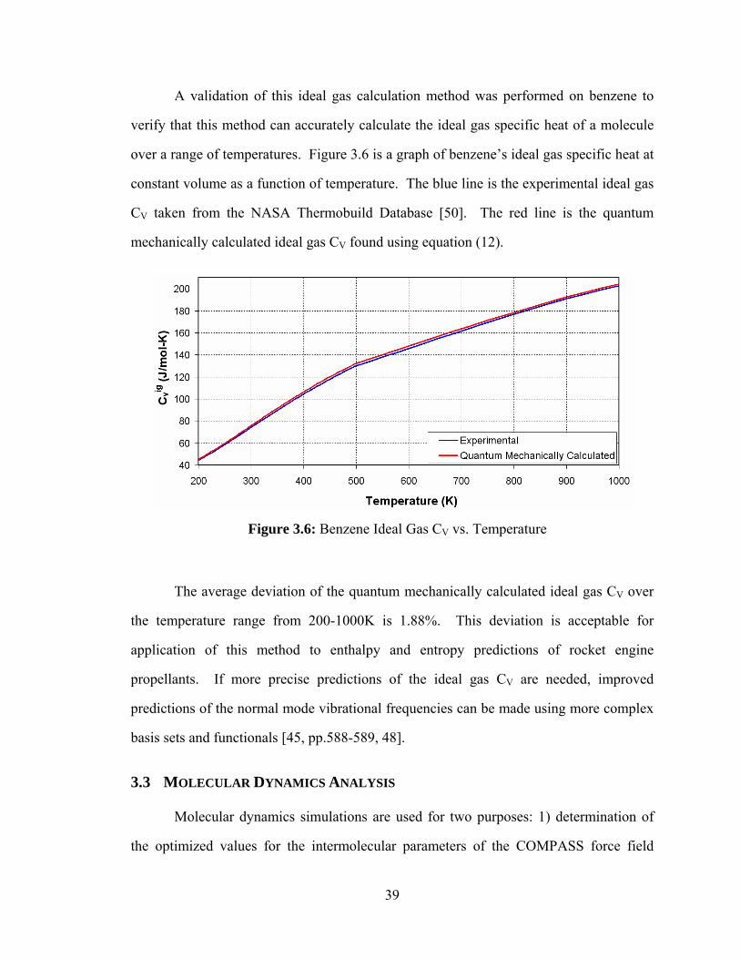
39
A validation of this ideal gas calculation method was performed on benzene to
verify that this method can accurately calculate the ideal gas specific heat of a molecule
over a range of temperatures. Figure 3.6 is a graph of benzene’s ideal gas specific heat at
constant volume as a function of temperature. The blue line is the experimental ideal gas
CV taken from the NASA Thermobuild Database [50]. The red line is the quantum
mechanically calculated ideal gas CV found using equation (12).
The average deviation of the quantum mechanically calculated ideal gas CV over
the temperature range from 200-1000K is 1.88%. This deviation is acceptable for
application of this method to enthalpy and entropy predictions of rocket engine
propellants. If more precise predictions of the ideal gas CV are needed, improved
predictions of the normal mode vibrational frequencies can be made using more complex
basis sets and functionals [45, pp.588-589, 48].
3.3 MOLECULAR DYNAMICS ANALYSIS
Molecular dynamics simulations are used for two purposes: 1) determination of
the optimized values for the intermolecular parameters of the COMPASS force field
Figure 3.6: Benzene Ideal Gas CV vs. Temperature

40
model (last two terms in equation (2)), and 2) calculation of the enthalpy, entropy, and
density of the HEDM molecule of interest over the entire range of temperature and
pressure experienced in a liquid rocket engine.. The COMPASS (Condensed-phase
Optimized Molecular Potentials for Atomistic Simulation Studies) model, as the name
implies, is a molecular force field model that is optimized for condensed-phases
[8,51,52,53]. This model is particularly useful for predicting thermophysical properties
for rocket propellants because the propellant is normally in a condensed phase for the
majority of the time it flows through the different engine components. Figure 3.7 shows
a snapshot of a molecular dynamics simulation of one such potential rocket propellant
and HEDM molecule, liquid DMAZ. The blue atoms are nitrogen, the cyan atoms are
carbon, and the white atoms are hydrogen.
Figure 3.7: Molecular Dynamics Snapshot of Liquid DMAZ

41
Molecular dynamics is used initially to determine the appropriate values for the
parameters used in the intermolecular terms of the COMPASS model. These terms
describe the intermolecular potential (potential between two atoms in different molecules
or two atoms in the same molecule not connected through a bond, angle, or dihedral).
Molecular dynamics is used in conjunction with experimental data to determine
these parameter values. Due to the fact that little or no experimental data is known for
the HEDM propellant of interest, a model compound is used in this step of the method.
A model compound should be chosen based on the following rules:
Rule 1: The model compound must have a “similar” molecular structure as
the corresponding HEDM compound.
In this rule, “similar” refers to a comparable molecular geometry and bond
structure. For quadricyclane, this means that the model compound must also be a
hydrocarbon with a bicyclic structure. For DMAZ, the model compound must have an
azide chain (three nitrogen atoms bonded together).
Rule 2: The model compound must have the same atom types as the HEDM
compound.
Atom types are defined in molecular dynamics as an element plus some
distinguishing bonding characteristics [8]. For instance, quadricyclane (see Figure 3.8) is
defined by three types: two carbon atom types and one hydrogen atom type. The
hydrogen atom type, denoted h1, is a nonpolar hydrogen. The first carbon atom type,
denoted c4, is a generic sp3 carbon. The top carbon atom in Figure 3.8 is a c4 carbon.
The second carbon atom type, denoted c43, is a sp3 carbon with three heavy atoms
attached. The remaining carbon atoms in Figure 3.8 are c43 carbons.

42
Rule 3: The model compound must have some density and enthalpy (or
specific heat) experimental data in the liquid phase.
This rule is necessary because the intermolecular parameters are optimized in
order to match the experimentally measured density and specific heat in the liquid phase.
Armed with a model compound chosen based upon these rules, molecular
dynamics simulations of the model compound are compared with the corresponding
experimental data.
Once the intermolecular parameters have been optimized, they are used for
molecular dynamics simulations of the HEDM compound at temperatures and pressures
experienced in a liquid rocket engine. Enthalpy change, entropy change, and density are
computed at each temperature and pressure combination. These results can be imported
into liquid rocket engine powerhead design codes and then used to perform conceptual
engine designs using these HEDM propellants.
A potential drawback of this technique of using the optimized intermolecular
parameters on a wide temperature and pressure range of molecular dynamics simulations
of HEDM compounds is that the parameter optimization is based upon DOE runs at a
single liquid temperature and pressure (typically 298 K and 1 atm). An assumption is
Figure 3.8: Ball and Cylinder Rendering of Quadricyclane (C7H8)

43
made that one can optimize the intermolecular parameters for a single temperature and
pressure combination, and then use those optimized parameters for molecular dynamics
simulations at significantly different temperature and pressure combinations.
Molecular dynamics simulations of benzene using the baseline COMPASS model
were performed over a wide range of pressures to examine the ability of the COMPASS
parameters, optimized for the prediction of properties of liquid compounds at 298 K and
1 atm., to accurately predict thermophysical properties at vastly different pressures. The
results of these simulations are provided in Figure 3.9 – Figure 3.11. The results indicate
that molecular dynamics can accurately predict the thermophysical properties of
substances even when the simulated pressure is significantly different than the one used
to optimize the intermolecular potential parameter values. Adding the enthalpy and
entropy of formation of liquid benzene to the sensible enthalpies and entropies calculated
from the molecular dynamics simulations, the average RMS deviations for density, total
enthalpy, and total entropy are provided in Table 3.1. The enthalpy and entropy of
formation of liquid benzene are 11.81 kcal/mol and 41.57 cal/mol-K respectively [39].
Figure 3.9: Benzene Density vs. Pressure (T = 298 K)

44
COMPASS Average RMS Deviation Density 0.18% Total Enthalpy 0.13% Total Entropy 0.12%
Figure 3.10: Benzene Sensible Enthalpy vs. Pressure (T = 298 K)
Figure 3.11: Benzene Sensible Entropy vs. Pressure (T = 298 K)
Table 3.1: Average RMS Deviations of MD Benzene Property Predictions

45
The results shown in Table 3.1 indicate that it is fair to assume that one can use
the intermolecular force field parameters optimized at one temperature and pressure for
molecular dynamics condensed phase simulations at significantly different pressures.
3.3.1 DESCRIPTION OF KEY MOLECULAR DYNAMICS ISSUES
There are several key issues that need to be understood when performing
molecular dynamics calculations. These include periodic boundary conditions, long-
range cutoffs and corrections terms, time-step sizes and number of time-steps, and the
different types of molecular dynamics simulations.
Periodic boundary conditions are a technique of surrounding the computational
domain with exact replicas of the computational domain. This technique is useful in
simulating thermodynamic properties that are based upon a continuum fluid [31]. Figure
3.12 is a schematic of this idea [10]. The central box is the computational domain and all
the surrounding boxes are exact replicas, or images, of the central box.
Long-range cutoffs allow the simulations to avoid detailed calculations of the
intermolecular potential between a pair of atoms that are far apart. Long-range cutoffs
are used in order to greatly speed up simulations, because all intermolecular potential
calculations between two atoms outside the cutoff distance are ignored [54, pp.64-65].
Cutoff distances can be used because the intermolecular potential rapidly approaches zero
at large distances (see Figure 2.4). Figure 3.13 is a schematic of the idea of a long-range
Figure 3.12: Schematic of Periodic Boundary Conditions in Two Dimensions

46
cutoff. The blue atom in the center has a long-range cutoff distance of rLRC for all
intermolecular potential calculations. The intermolecular potentials between the blue
atom and the green atoms within the dotted circle are calculated. The intermolecular
potentials between the blue atom and the red atoms outside of the dotted circle are not
calculated. In this simple case, this reduces the number of intermolecular calculations
between the blue atom and the rest of the atoms from seven (four red and three green) to
three.
Long-range energy and pressure corrections are used to account for the potential
not modeled outside the long-range cutoff distance [31]. For the van der Waals
intermolecular potential term (the last term in equation (2)), a simple analytically
determined correction is applied to the overall energy and pressure of the system. The
equations below are the long-range energy and pressure corrections to the van der Waals
potential energy [8].
(18)
(19)
Figure 3.13: Schematic of a Long-Range Cutoff in Two Dimensions
rLRC
∑ ∑ ∫= =
∞
=n
i
n
j rijjiLRC
LRC
drr)r(ENE1 1
2421 πρ
∑ ∑ ∫= =
∞
⎟⎟⎠
⎞⎜⎜⎝
⎛=
n
i
n
j r
ijjiLRC
LRC
drdr
)r(dErP
1 1
3461 πρρ

47
In the above equations, n is the number of different intermolecular atom types
(described earlier in section 3.3) interacting with an intermolecular pair potential Eij(r).
Ni is the number of atoms of atom type i and ρi is the density of atom type i. The variable
r is the distance between the two atoms whose intermolecular pair potential is being
calculated.
The long range Coulomb interactions are modeled using the particle-particle,
particle-mesh technique [10,55,38]. Coulomb interactions are a result of the charges
associated with two atoms i and j (term 11 of equation (2)). This technique for modeling
Coulomb interactions is an efficient means of modeling these interactions without
utilizing a cutoff distance. A cutoff distance was not used for modeling Coulomb
interactions due to the fact that these interactions extend a much larger distance than do
van der Waals interactions. As seen in term 11 of equation (2), the Coulomb potential is
proportional to r -1 as opposed to r -6 for van der Waals interactions (term 12 of equation
(2)).
Two different types of molecular dynamics simulations are utilized for this
research work. The first type is a constant number of particles (N), constant volume (V),
constant temperature (T) simulation. This type of simulation is known as an NVT
simulation [54, pp.40-41]. The second type is a constant number of particles, constant
pressure (P), constant temperature (NPT) simulation [54, pp.41-42].
For each molecular dynamics run performed for this research work, the following
steps were used.
1. An initial molecular configuration is input (typically a grid of 125 molecules
lined up along the three Cartesian axes).
A study of the prediction of density and intermolecular potential energy as a
function of the number of molecules simulated was performed in order to determine the
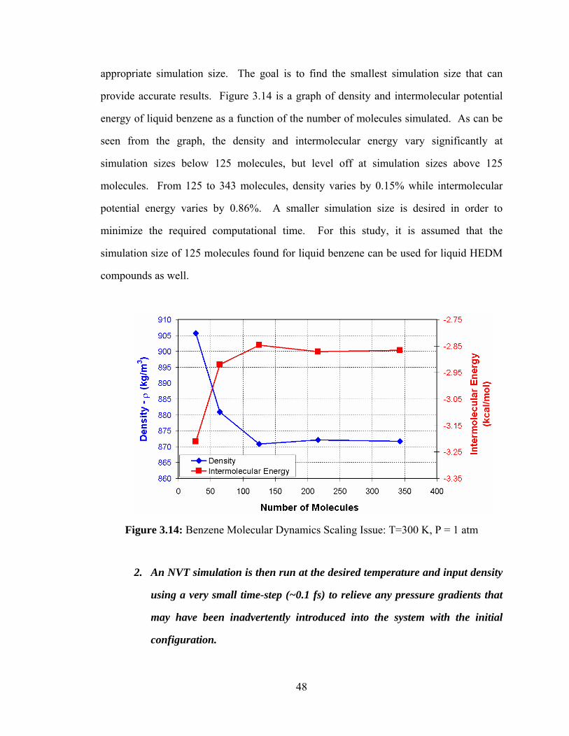
48
appropriate simulation size. The goal is to find the smallest simulation size that can
provide accurate results. Figure 3.14 is a graph of density and intermolecular potential
energy of liquid benzene as a function of the number of molecules simulated. As can be
seen from the graph, the density and intermolecular energy vary significantly at
simulation sizes below 125 molecules, but level off at simulation sizes above 125
molecules. From 125 to 343 molecules, density varies by 0.15% while intermolecular
potential energy varies by 0.86%. A smaller simulation size is desired in order to
minimize the required computational time. For this study, it is assumed that the
simulation size of 125 molecules found for liquid benzene can be used for liquid HEDM
compounds as well.
2. An NVT simulation is then run at the desired temperature and input density
using a very small time-step (~0.1 fs) to relieve any pressure gradients that
may have been inadvertently introduced into the system with the initial
configuration.
Figure 3.14: Benzene Molecular Dynamics Scaling Issue: T=300 K, P = 1 atm

49
NVT simulations typically require 100,000 time-steps to relieve any initial
pressure gradients.
3. An NPT simulation is then used to gather energy and density data at the
desired temperature and pressure. The time-step used for NPT simulations
is typically between 0.2 fs and 1.0 fs.
Pressure is not controlled during NVT simulations and is, therefore, generally not
the same pressure as that desired during NPT simulations. As a result, at the start of NPT
simulations the calculated pressure is substantially different from the desired pressure.
Therefore NPT simulations typically require 600,000 to 1 million time-steps to converge
to a stable pressure, temperature, and volume. Once convergence has been reached,
another 500,000 to 2 million time-steps are run in NPT mode and statistics are collected.
Figure 3.15 and Figure 3.16 are graphs showing the convergence history of the calculated
density and total enthalpy respectively of a liquid quadricyclane molecular dynamics
simulation.
As can be seen from these figures, approximately 600,000 time steps are required
for the calculated density to converge to its final solution. Total energy converges more
quickly (~500,000 time steps). Once convergence has been achieved, both high
frequency and low frequency fluctuations still occur. The average of over 1 million time
steps is used to compute the density for a particular molecular dynamics simulation. In
the case of Figure 3.15, the average is taken from time step 600,000 to time step 2.2
million. The temperature and energy are also averaged over this simulation period and
those results are the ones recorded for use in enthalpy, entropy, and density predictions.

50
Figure 3.15: Density vs. Time-Step for Quadricyclane
Figure 3.16: Total Energy vs. Time-Step for Quadricyclane

51
3.3.2 FITTING INTERMOLECULAR PARAMETERS
Molecular dynamics is used initially to fit the intermolecular parameters. This is
done by comparing the results of MD simulations with experimental data and adjusting
the intermolecular parameters of the force field function in order to better match
experimental data. For this work, the experimental data of interest is the density and
specific heat of the model compound as a function of temperature and pressure.
The intermolecular potential parameters are initially set using a 6th order
combination law for unlike atom pairs (two atoms of different atom types) shown in the
equations below. Parameter values for like atom pairs (two atoms of the same atom type)
are known from published results [8,9,18,19,51,53]. Parameter values for unlike atom
pairs can be computed very quickly using the equations below.
(20)
(21)
In the above equations, σi is the Lennard-Jones-9-6 parameter for atom i, σj is the
Lennard-Jones-9-6 parameter for atom j, εi is the energy potential well depth for atom i, εj
is the energy potential well depth for atom j, and σij and εij are combinations for a pair of
atoms i and j. The two combination parameters σij and εij are used in the last two terms
of the COMPASS model shown in equation (2). The term Lennard-Jones refers to the
potential upon which these parameters are used. The Lennard-Jones-9-6 potential, which
is the last term of the COMPASS model, can and has been used by itself as a potential
function. It is effective in modeling simple molecules and was originally used in the
1960’s for the modeling of liquid argon [10].
( ) ( ) 61
66
2 ⎥⎥⎦
⎤
⎢⎢⎣
⎡ += ji
ij
σσσ
( ) ( )( ) ( ) ⎥
⎥⎦
⎤
⎢⎢⎣
⎡
+= 66
33
2ji
jijiij σσ
σσεεε

52
3.3.3 DESIGN OF EXPERIMENTS
A design of experiments (DOE) is performed on the intermolecular parameters to
determine the sensitivity of density to changes in these parameters. DOE techniques are
a structured approach for changing design variable settings (in the case of this work, the
design variables are σij and εij) and observing the resulting response (in the case of this
work, the response is density) [56, pp.549-550]. The DOE used in this work is the central
composite design (CCD) [56, pp.645-650].
For a molecule with two atom types, there are four design variables (σ and ε for
each atom type). A four design variable CCD run list results in 27 runs (with three center
points) and is shown in Table 3.2 below. The ‘0’ settings in Table 3.2 represent the
baseline value for the particular design variable. The ‘+1’ settings represent the baseline
value plus some perturbation. In the case of this molecular dynamics work, this
perturbation typically was 10% of the baseline σ or ε value. The ‘-1’ settings represent
the baseline value minus the same perturbation.
The first 16 runs are a full factorial array. The number of runs in a full factorial
array is equal 2N where N equals the number of design variables. Runs 17-24 are the star
points. Star points are designs within a CCD which have only a single variable altered
from the baseline value. Runs 25-27 are the center points. The center points are designs
with all design variable settings set at the baseline values. Multiple center points are used
in general when the process or program being run has some variability. In the case of
molecular dynamics, the initial velocity vectors of the molecules are computed using a
random number generator with a random number seed. The three center points each have
a different random number seed and result in slightly different simulation results. The
JMP Statistical Discovery Software tool [57] was used to create all DOE run lists used
for this research work.
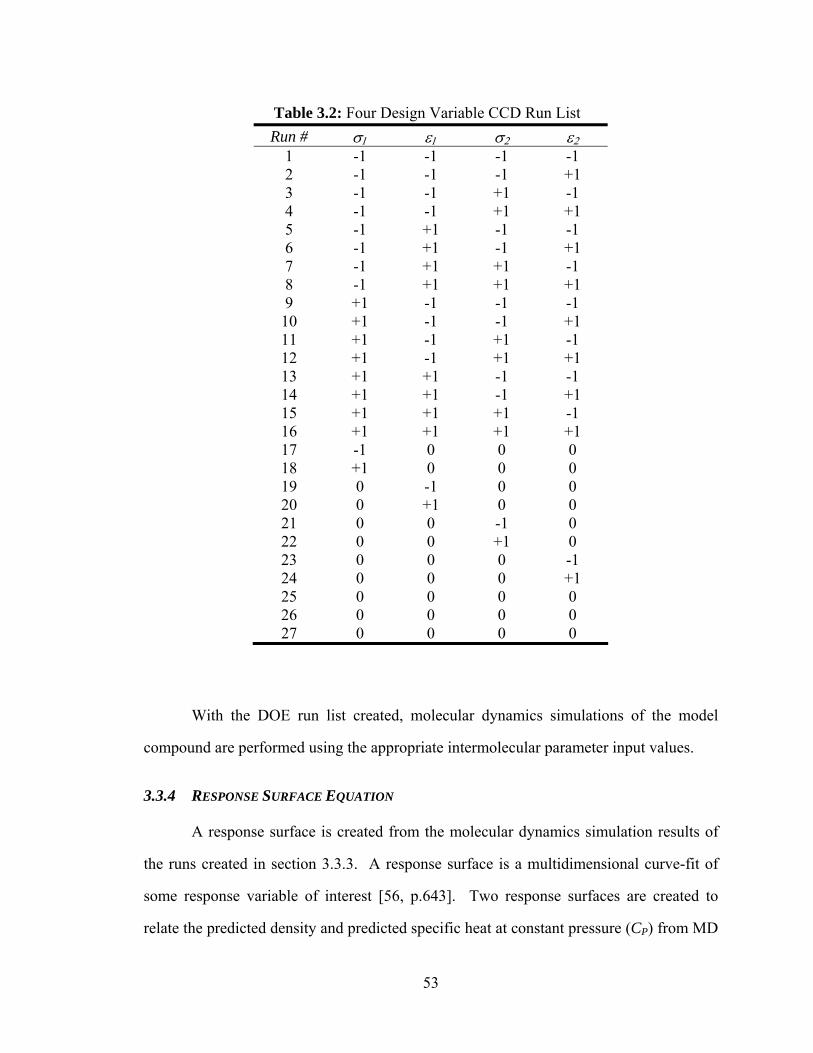
53
With the DOE run list created, molecular dynamics simulations of the model
compound are performed using the appropriate intermolecular parameter input values.
3.3.4 RESPONSE SURFACE EQUATION
A response surface is created from the molecular dynamics simulation results of
the runs created in section 3.3.3. A response surface is a multidimensional curve-fit of
some response variable of interest [56, p.643]. Two response surfaces are created to
relate the predicted density and predicted specific heat at constant pressure (CP) from MD
Table 3.2: Four Design Variable CCD Run List Run # σ1 ε1 σ2 ε2
1 -1 -1 -1 -1 2 -1 -1 -1 +1 3 -1 -1 +1 -1 4 -1 -1 +1 +1 5 -1 +1 -1 -1 6 -1 +1 -1 +1 7 -1 +1 +1 -1 8 -1 +1 +1 +1 9 +1 -1 -1 -1 10 +1 -1 -1 +1 11 +1 -1 +1 -1 12 +1 -1 +1 +1 13 +1 +1 -1 -1 14 +1 +1 -1 +1 15 +1 +1 +1 -1 16 +1 +1 +1 +1 17 -1 0 0 0 18 +1 0 0 0 19 0 -1 0 0 20 0 +1 0 0 21 0 0 -1 0 22 0 0 +1 0 23 0 0 0 -1 24 0 0 0 +1 25 0 0 0 0 26 0 0 0 0 27 0 0 0 0
54
simulations to the settings for the intermolecular parameters. The response surface
equation (RSE) used is a second order response surface which includes all first order
effects and all second order effects, including cross terms. For the four design variable
example discussed in 3.3.3, this results in the following RSE for density:
(22)
(23)
In equation (22), the σ and ε multipliers are normalized values based upon
equation (23). These values are normalized based upon the maximum and minimum
settings for each multiplier. In the example discussed in 3.3.3, the maximum and
minimum values are +1 and -1. This normalization is performed to help compensate for
severe differences in the magnitude of each design variable in the RSE. This enables the
user to quickly see the relative importance of a particular term in the RSE by looking at
the magnitude of the βi’s.
A similar RSE is created for the predicted specific heat at constant pressure from
MD simulation results. In the above equation, the βρi values are coefficients calculated
from the DOE simulation run results using a least squares fit. These coefficient values
are calculated using the JMP software. In this example, 14 coefficients are created using
a DOE with 27 runs. JMP also calculates the goodness of fit, or R2 value, for the RSE.
The R2 value is a measure of how well the RSE approximates the responses from the
DOE runs [56:323]. The equation for R2 is provided below:
(24)
22142113211221112110119
228
227
216
215242312110
εσβεεβσεβεσβσσβεσβ
εβσβεβσβεβσβεβσββρ
ρρρρρρ
ρρρρρρρρρ
+++++
+++++++++=
total
error
SSSSR −= 12
( )1
2−
−−
= mini
maxi
minii
i σσσσ
σ
55
In the above equation, SSerror is the sum of squares for error [58, p.542] and SStotal
is the total sum of squares [58, p.543]. The closer R2 is to a value of 1, the better the RSE
approximates the molecular dynamics results. The RSEs created for this research work
have R2 values between 0.90 and 0.99.
3.3.5 OPTIMIZATION AND VALIDATION
Once the RSEs for density and specific heat are created, the intermolecular
variable values are optimized. The goal of the optimization is to match the RSE
predicted density and specific heat values with experimental results. The objective
function for the optimizer is:
(25)
In equation (25), xi is the current value for the multiplier for the ith intermolecular
parameter and N is the number of intermolecular parameters. When the intermolecular
parameters are set to their baseline values, the xi’s are all equal to 1. This optimization is
subject to the following constraint:
(26)
In equation (26), M is the number of (T, P) combinations modeled, ρpredicted_i and
CPpredicted_i are the RSE predicted values for density and specific heat at the ith (T, P)
combination. The variables ρactual_i and CPactual_i are the experimentally measured values
for density and specific heat at the ith (T, P) combination. Wρ_i and Wcp_i are the
weighting factors for the density and specific heat terms respectively for the ith (T, P)
combination. One may want to optimize the intermolecular parameters so that the
( )∑=
−=N
iixS
1
21
0
1
22
≤−⎥⎥⎥
⎦
⎤
⎢⎢⎢
⎣
⎡
⎟⎟⎠
⎞⎜⎜⎝
⎛ −+⎟
⎟⎠
⎞⎜⎜⎝
⎛ −= ∑
=
max
M
i i_actualP
i_actualPi_predictedPi_cp
i_actual
i_actuali_predictedi_
E
CCC
WWgρ
ρρρ

56
density is predicted very accurately at the expense of a less accurate prediction of specific
heat or optimize the intermolecular parameters so that a particular temperature and
pressure combination is predicted more accurately than others. For the first case, one
would make the density weighting factor larger than the specific heat weighting factor.
For the second case, one would make the weighting factors for the particular temperature
and pressure combination of interest larger than for the other combinations. Emax is the
maximum allowable weighted error. Typically, the smaller Emax is, the larger the
deviation from the baseline intermolecular parameters is required.
The optimized values for the intermolecular parameters are then used in
molecular dynamics simulations to validate the new parameter values. This is done to
verify that the RSEs did an adequate job at approximating the molecular dynamics
results. If the validation runs produce results that do not match the RSE predicted results,
additional terms may need to be added to the RSE to improve its approximation of the
molecular dynamics results. In this research work, additional terms were not needed to
improve the RSE prediction, but may, in general, be needed in some propellant analyses.
3.3.6 MOLECULAR DYNAMICS THERMOPHYSICAL PROPERTY CALCULATIONS
Molecular dynamics is used to compute the equilibrium properties of both the
model compound and the HEDM compound at a range of temperatures and pressures
[31,10]. This is done by expressing these equilibrium properties as a function of the
positions and momenta of the particles in the system.
The first observable that we define is the kinetic energy per particle. For a system
of point masses, the average kinetic energy of the system is defined using equation (27).
(27)
( )∑=
⋅=N
iiiikin vvmE
121 vv

57
In the above equation, N is the number of particles in the system and mi and ivv
are the respective mass and velocity of particle i. In the case of polyatomic molecules, mi
is the mass of the molecule and ivv is the velocity of the center of mass of the molecule.
From this definition of kinetic energy the average translational temperature of the system
of particles (in three-dimensional space) can be defined using equation (28):
(28)
where kB is Boltzmann’s constant. With the translational temperature defined, the
pressure can then be defined using equation (29).
(29)
where V is the volume of the computational space, αβijfv
is the force vector of atom β of
molecule j on atom α of molecule i, and αβijrv is the position vector from atom β of
molecule j to atom α of molecule i. The first term of equation (29) is the ideal gas term
while the second term is the configurational or “virial” term that becomes prominent at
higher densities (farther away from the ideal gas assumption). Density is defined as:
(30)
With these fundamental properties defined as a function of the positions and
momenta of the particles, more complex equilibrium properties can also be defined. For
example, the definition of enthalpy begins by dividing it into three components: enthalpy
of formation and ideal gas sensible enthalpy and residual sensible enthalpy,
( ) ( )⎟⎠
⎞⎜⎝
⎛⋅=⋅== ∑∑
==
N
iiii
B
N
iiii
BB
kintrans vvm
Nkvvm
NkNkE
T11 2
13
23
132 vvvv
∑ ∑ ∑∑−
= += = =
⋅+=1
1 1 1 131 N
i
N
ij
n n
ijijtransB rf
VVTNkP
α β
αβαβ vv
∑=
=N
iim
VN
1ρ

58
(31)
(32)
(33)
In equation (31), the enthalpy of formation, ∆hf0, is typically defined as the
enthalpy of the substance at 298K and 1 atm. with respect to the arbitrary basis elements
that make up that particle at the same temperature and pressure [24]. The second and
third terms in equation (31) are defined using the method developed by Lagache [40] and
Cadena et al. [41,42] for calculating the enthalpy of a liquid substance using quantum
mechanics and molecular dynamics.
The second term, igsensh , is the ideal gas sensible enthalpy defined previously in
equation (17). The ideal gas sensible enthalpy is based upon the normal mode vibrational
frequencies found from quantum mechanical analysis. The third term in equation (31),
the residual sensible enthalpy, ressensh , represents the condensed phase influence on the
sensible enthalpy. This term, found from molecular dynamics simulations, is based upon
the intermolecular energy (van der Waals and Coulombic) and the pressure divided by
the density. This method for calculating enthalpy is different from that suggested by
others [10,54] that attempts to calculate enthalpy using solely molecular dynamics
simulations. In this research work, it was found that the method developed by Lagache
and Cadena resulted in a more accurate prediction of specific heat, enthalpy, and entropy
than the method using only molecular dynamics.
Due to the fact that the intramolecular potential energy calculation (calculated
from the quantum mechanical analysis) and the intermolecular potential energy
calculation (calculated from molecular dynamics) are performed separately, any influence
)P,T(h)T(hh)P,T(h ressens
igsensf ++∆= 0
⎥⎦
⎤⎢⎣
⎡+−⎥
⎦
⎤⎢⎣
⎡+=
0
000 ρρ
P)P,T(EP)P,T(E)P,T(h interinter
ressens
)P,T(E)P,T(E)P,T(E coulvdwlinter +=

59
of one potential on the other is not captured using this method [40,41,42]. As a result, a
study was performed in order to capture of the influence of the intermolecular potential
energy on the intramolecular potential energy.
A series of NVT (constant number of particles, constant volume or density,
constant temperature) molecular dynamics simulations of benzene were performed and
the computed intermolecular and intramolecular energies were studied. The COMPASS
potential model was used for both intermolecular and intramolecular energies. Figure
3.17 is a graph of van der Waals intermolecular energy and total intramolecular energy as
a function of density for molecular dynamics simulations of benzene.
The results indicate that the intermolecular potential has very little influence on
the intramolecular potential (the intramolecular potential energy line is fairly flat over a
wide range of densities while the intermolecular potential energy varies significantly).
Over the range of densities studied the intramolecular potential energy changes by 1.56%.
This insensitivity of intramolecular potential to changes in intermolecular potential
indicates that the calculations of the two potentials can be performed separately with
Figure 3.17: Benzene Potential Energy Interaction Issue

60
minimal error [59] and thus the method developed by Lagache et al. [40] and Cadena et
al. [41,42] can be used in the prediction of enthalpy and specific heat.
The second equilibrium property defined is entropy. Entropy can be defined
similar to enthalpy by breaking up entropy into its two major components: entropy of
formation and sensible entropy:
(34)
The entropy of formation, ∆sf1atm, is typically defined as the entropy of the
substance at 298K and 1 atm. The entropy of a substance is normally defined to be zero
at 0K. The second term, ssens, is known as the sensible entropy and is defined as the
difference in entropy between any given state and the state at which the formation
entropy is defined. The entropy of formation of the molecule of interest is taken from the
quantum mechanics energy calculation code GAMESS. The sensible entropy for a
simple compressible substance is defined with the following “T ds” relation [60, p.236]:
(35)
Dividing through by the temperature, we get:
(36)
Using the chain rule [61, p.944], ds can be broken up into temperature and pressure
differentials with the following equation:
(37)
)P,T(ss)P,T(s sensatm
f +∆= 1
ρdPdhdP*vdhds*T −=−=
TdP
Tdhds
ρ−=
dPTT
dTTT
dPT
dPT
dTds TP
hPT
hTP
hPT
h
⎥⎥⎦
⎤
⎢⎢⎣
⎡−+
⎥⎥⎦
⎤
⎢⎢⎣
⎡=−+= ∂
∂∂
∂∂
∂∂
∂
ρρ1

61
Due to the fact that the definition of the change in entropy from one state
(temperature and pressure point) to another is path independent [62, pp.33-36], we define
ssens(T1,P1) with the following equation:
(38)
where T0 and P0 are the temperature and pressure at which the entropy of formation is
defined (298 K and 1 atm) and s(T0, P0) is the entropy of formation, ∆sf1atm. Figure 3.18
is a graphical representation of the process used for calculating sensible enthalpy. With
enthalpy defined at T0 and P0, the entropy change is first calculated for a constant
pressure process from (T0, P0) to (T1, P0). The entropy change is then calculated for a
constant temperature process from (T1, P0) to (T1, P1), the desired temperature and
pressure.
Using equation (37), the constant pressure process from (T0, P0) to (T1, P0) is
defined as follows [63, p.534]:
Figure 3.18: Process of Calculating Entropy Change
( ) ( )[ ] ( ) ( )[ ]0111000111 P,TsP,TsP,TsP,Ts)P,T(ssens −+−=
Temperature, T
Pres
sure
, P
s(T0,P0) s(T1,P0)
s(T1,P1)
Constant P process
Constant T process

62
(39)
The constant temperature process from (T1, P0) to (T1, P1) is defined as follows:
(40)
These equations can be numerically integrated to calculate the total entropy as a function
of temperature and pressure in order to create property data tables for rocket engine
design codes.
3.3.7 ENTHALPY, ENTROPY, AND DENSITY DATA TABLE CREATION
Molecular dynamics runs of the HEDM compounds are performed using the
updated intermolecular parameters to populate the data tables needed for rocket engine
design codes. Molecular dynamics simulations are performed at appropriate temperature
and pressure combinations for rocket engine analysis. The temperature and pressure
combinations are chosen to cover the entire range of temperatures and pressures that the
HEDM propellant will experience while flowing through the different engine
components.
An example REDTOP-2 [64] propellant input file format is shown in Figure 3.19.
For REDTOP-2, the top of the input file defines the molecule (number of atoms of each
element and molecular weight). Also included are some data specification options, the
number of pressures and temperatures included in the data file, and whether or not
REDTOP-2 should calculate the gaseous density using the perfect gas equation. After
this top part of the input file is defined, the rest of the input file is a table of
thermophysical properties. The thermophysical properties calculated by molecular
dynamics simulations are placed in this part of the REDTOP-2 propellant input file.
( ) ( ) ( )∫ ∫ ∫=
⎥⎥⎦
⎤
⎢⎢⎣
⎡==− ∂
∂1
0
1
0
1
0
00001
T
T
T
T
T
T
PPTh
dTT
P,TcdT
TdsP,TsP,Ts
( ) ( ) ( )∫ ∫⎥⎥⎦
⎤
⎢⎢⎣
⎡−==− ∂
∂1
0
1
0 1110111
1P
P
P
P
TPh
dPTP,TT
dsP,TsP,Tsρ

63
Special attention must be paid to the units for each thermophysical property to avoid a
unit conversion error.
3.4 ADDITIVITY METHODS
The third and final part of the thermophysical property calculation method is the
use of additivity methods to determine the kinematic viscosity and thermal conductivity
of the compounds of interest. Additivity methods are used instead of molecular dynamics
for these two properties based upon the results of the sensitivity study discussed in
Chapter 1. In this sensitivity study, it was shown that Isp is fairly insensitive to changes
Figure 3.19: Sample REDTOP-2 Propellant Input File
Species_Name CH4 Number_Atoms 2 Atoms(1) C Atoms_Value(1) 1 Atoms(2) H Atoms_Value(2) 4 Molecular_Weight: 16.043 Data_Specification_Option 7 Number_Pressures 601 Number_Temperatures 25 Use_Perfect_Gas_Density No T(R) P(psi) ρ(lbm/ft3) h(BTU/lbm) s(BTU/lbm-R) k(BTU/ft-hr-R) µ(lbm/ft-s) 175 0 27.636 -2420.7 1.062 0.11752 0.00011301 175 25 27.643 -2420.6 1.0618 0.1176 0.00011321 175 50 27.651 -2420.5 1.0615 0.11769 0.00011345 175 75 27.659 -2420.3 1.0612 0.11779 0.00011369 175 100 27.666 -2420.2 1.0609 0.11788 0.00011393 175 125 27.674 -2420.1 1.0606 0.11798 0.00011416

64
in kinematic viscosity and thermal conductivity. As a result, the predictions of kinematic
viscosity and thermal conductivity do not need to be as accurate as the predictions of
enthalpy, entropy, and density.
While not the only parameter affected by these properties, Isp is the most
important. Kinematic viscosity and thermal conductivity are important parameters in the
calculation of pump efficiency and propellant feed line pressure losses [65]. These both
contribute to the weight estimation of engine components. However, these effects are
small compared to the effect of Isp when examining vehicle level metrics like gross
vehicle weight.
As discussed in Chapter 2, additivity methods make use of the observation that a
substance’s physical properties depend on that substance’s particular molecular structure
[26,28, p.24]. The additivity methods used in this work were developed by Chung et al.
[66]. Chung’s method is a general multiparameter correlation that can be used to predict
the viscosity and thermal conductivity of a wide range of hydrocarbons in the liquid,
supercritical, and gaseous states and are based upon an input temperature and density
[66]. Chung found the average absolute deviation for condensed phase shear viscosity to
be 4% and for condensed phase thermal conductivity to be 8.6% for the hydrocarbons
upon which Chung’s correlations are based [66].
The temperature range in which the additivity methods are used in this work is the
same temperature range used for the molecular dynamics simulations of the HEDM
compound. The densities used as input into the additivity method model come from the
computed densities from the molecular dynamics simulations at the desired temperature
and pressure.

65
3.4.1 DESCRIPTION AND IMPLEMENTATION OF CHUNG’S METHOD
Chung’s additivity methods extend the additivity work performed by Chapman
and Cowling [67] for dilute gas viscosity and thermal conductivity. Chung lists the
following equations for the calculation of the dilute gas shear viscosity:
(41)
In equation (41), η0 is the dilute gas shear viscosity in P, M is the molecular
weight in g/mol, T is the temperature in Kelvin, Vc is the critical volume in cm3/mol, Fc
and Ω* are empirical coefficients defined with the following equations:
(42)
(43)
The empirical coefficients in the W* equation are defined by Neufield et al. [68]
and equal defined as: A=1.16145, B=0.14874, C=0.52487, D=0.77320, E=2.16178,
F=2.43787, G=-6.435*10-4, H=7.27371, S=18.0323, and W=-0.76830. In the above
equations, ω is the acentric factor, T* is the dimensionless temperature defined with the
following equation:
(44)
where kB is Boltzmann’s constant and ε is the potential energy parameter, which is related
to the critical temperature, Tc (Kelvin), with the following equation:
( ) ( )c/
c
.
F*V
MT.Ω
×= −32
505
0 1007854η
( ) ( ) ( )H*STsin*GT*FTexp
E*DTexp
C*TA* WB
B −+++=Ω
ω275601 .Fc −=
εTk*T B=

66
(45)
The acentric factor, w, is defined by Pitzer [69] to equal:
(46)
where Pvap is the vapor pressure at T = 0.7*Tc, the critical temperature (Kelvin) and Pc is
the critical pressure. The above list of equations is based upon the critical point of the
substance of interest (critical density, temperature, and pressure). For this research work,
the critical point is taken from literature values if available. If these values are not
available in the literature, then the critical point is predicted using Joback’s group
contributions [70]. The equations used by Joback for computing the boiling temperature
and the critical point are provided below:
(47)
(48)
(49)
(50)
In the above equations, Tb is the boiling point temperature in K, Tc is the critical
temperature in K, Pc is the critical pressure in bar, Vc is the critical volume in liters/kmol,
25931.kT Bc=ε
⎟⎟⎠
⎞⎜⎜⎝
⎛−−=
c
vap
PP
log101ω
∑+= onscontributi_bb TT 198
( )296505840 ∑∑ −+=
onscontributi_conscontributi_c
bc
TT..
TT
∑−+=
onscontributi_cc Pn..
P003201130
1
∑+= onscontributi_cc V.V 517

67
n is the number of atoms in the molecule of interest, and the summations are all group
contributions of different atoms and groups in the molecule of interest. Table 3.3 lists the
group contributions developed by Joback [70].
Tc Pc Vc Tb Nonring Increments
-CH3 0.0141 -0.0012 65 23.58 -CH2- 0.0189 0.0000 56 22.88 >CH- 0.0164 0.0020 41 21.74 >C< 0.0067 0.0043 27 18.25 =CH2 0.0113 -0.0028 56 18.18 =CH- 0.0129 -0.0006 46 24.96 =C< 0.0117 0.0011 38 24.14 =C= 0.0026 0.0028 36 26.15 ≡CH 0.0027 -0.0008 46 9.20 ≡C- 0.0020 0.0016 37 27.38
Ring Increments -CH2- 0.0100 0.0025 48 27.15 >CH- 0.0122 0.0004 38 21.78 >C< 0.0042 0.0061 27 21.32
=CH- 0.0082 0.0011 41 26.73 =C< 0.0143 0.0008 32 31.01
Nitrogen Increments -NH2 0.0248 0.0109 36 73.23
>NH (nonring) 0.0295 0.0077 35 50.17 >NH (ring) 0.0130 0.0114 29 52.82
>N- (nonring) 0.0169 0.0074 9 11.74 -N= (nonring) 0.0255 -0.0099 0 74.60
-N= (ring) 0.0085 0.0076 34 57.55 -CN 0.0496 -0.0101 91 125.66 -NO2 0.0437 0.0064 91 152.54
The dilute gas thermal conductivity is defined based upon the dilute gas shear
viscosity using the following equations:
(51)
(52)
(53)
Table 3.3: Joback Group Contributions [70]
( )Ψ= M/. 00 4527 ηλ
αβββαα
061163660266650061128288021501
.Z.Z....
+++−+
+=Ψ
23 /Rcv −=α

68
(54)
(55)
In the above equations, λ0 is the dilute gas thermal conductivity in cal/cm-s-K, cv is the
ideal gas heat capacity at constant volume in cal/mol-K, and R is the ideal gas constant
(1.987 cal/mol-K).
The dilute gas shear viscosity and thermal conductivity are then used to compute
the condensed phase shear viscosity and thermal conductivity [66]. The following
relations are used to calculate the condensed phase shear viscosity:
(56)
(57)
(58)
(59)
(60)
(61)
In the above equations, η0 is the dilute gas viscosity. The constants A1 through A10 are
defined with the following equation and Table 3.4 below:
2316817109078620 ωωβ ... +−=
2
51002 ⎟⎟⎠
⎞⎜⎜⎝
⎛+=
cTT..Z
pk ηηη +=
( )YAG/k 620 1 += ηη
( ) ( )210982
2732
5051063443*T/A*T/AAexpGYA
VMT.
/c
.c
p ++⎥⎥⎦
⎤
⎢⎢⎣
⎡ ×=
−
η
6cV
Yρ
=
( )31 15001
YY..G
−−
=
( )[ ] ( )3241
13512412
1AAAA
GAYAexpGAY/YAexpAG
++++−−
=

69
(62)
i a0(i) a1(i) 1 6.32402 50.4119 2 1.21E-03 -1.15E-03 3 5.28346 254.209 4 6.62263 38.0957 5 19.7454 7.63034 6 -1.89992 -12.5367 7 24.2745 3.44945 8 0.79716 1.11764 9 -0.23816 6.77E-02
10 6.86E-02 0.34793
The condensed phase thermal conductivity is defined in a similar manner as the
condensed phase shear viscosity. The following equations are used to define the
condensed phase thermal conductivity:
(63)
(64)
(65)
(66)
In the above equations, λ0 is the dilute gas thermal conductivity. The constants B1
through B7 are defined with the following equation and Table 3.5 below:
(67)
Table 3.4: Constants Used for Condensed Phase Shear Viscosity Relation [66]
ω)i(a)i(aAi 10 +=
( )YBH/k 620 1 += λλ
( ) 50
22
732
504100393.
c/
c
.c
p TTHYB
VM/T.
⎟⎟⎠
⎞⎜⎜⎝
⎛
⎥⎥⎦
⎤
⎢⎢⎣
⎡ ×=
−
λ
( )[ ] ( )3241
13512412
1BBBB
GBYBexpGBY/YBexpBH
++++−−
=
pk λλλ +=
ω)i(b)i(bBi 10 +=
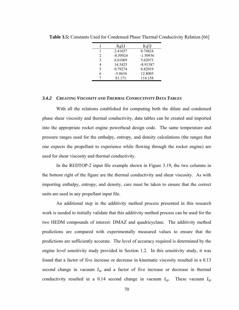
70
i b0(i) b1(i) 1 2.41657 0.74824 2 -0.50924 -1.50936 3 6.61069 5.62073 4 14.5425 -8.91387 5 0.79274 0.82019 6 -5.8634 12.8005 7 81.171 114.158
3.4.2 CREATING VISCOSITY AND THERMAL CONDUCTIVITY DATA TABLES
With all the relations established for computing both the dilute and condensed
phase shear viscosity and thermal conductivity, data tables can be created and imported
into the appropriate rocket engine powerhead design code. The same temperature and
pressure ranges used for the enthalpy, entropy, and density calculations (the ranges that
one expects the propellant to experience while flowing through the rocket engine) are
used for shear viscosity and thermal conductivity.
In the REDTOP-2 input file example shown in Figure 3.19, the two columns in
the bottom right of the figure are the thermal conductivity and shear viscosity. As with
importing enthalpy, entropy, and density, care must be taken to ensure that the correct
units are used in any propellant input file.
An additional step in the additivity method process presented in this research
work is needed to initially validate that this additivity method process can be used for the
two HEDM compounds of interest: DMAZ and quadricyclane. The additivity method
predictions are compared with experimentally measured values to ensure that the
predictions are sufficiently accurate. The level of accuracy required is determined by the
engine level sensitivity study provided in Section 1.2. In this sensitivity study, it was
found that a factor of five increase or decrease in kinematic viscosity resulted in a 0.13
second change in vacuum Isp and a factor of five increase or decrease in thermal
conductivity resulted in a 0.14 second change in vacuum Isp. These vacuum Isp
Table 3.5: Constants Used for Condensed Phase Thermal Conductivity Relation [66]
71
sensitivities are for a staged-combustion cycle rocket engine. It is expected that vacuum
Isp is more sensitive to changes in kinematic viscosity and thermal conductivity for
expander cycle engines, but not a great deal more.
As a result, in order to keep the error in vacuum Isp due to errors in kinematic
viscosity and thermal conductivity under 0.25 seconds (an acceptable error in predicted
vacuum Isp for conceptual vehicle design), a conservative error of 150% is deemed
acceptable in the additivity method predictions of kinematic viscosity and thermal
conductivity.
3.5 EXPERIMENTAL METHODS
In general application of the method developed in this thesis work, little or no
experimental testing is needed. This is because the method uses previously published
experimental data from model compounds to determine the appropriate settings for the
intermolecular potential parameters.
For this thesis research, however, validation of the computational results from the
quantum mechanical, molecular dynamics, and group additivity method analyses is
necessary. This validation is done by comparing the computational results with
experimentally measured thermophysical properties. Experimental data for
quadricyclane was previously published by Wucherer et al. [1]. However, very little
published experimental data exists for the other HEDM compound of interest, DMAZ.
As a result, experimental testing of DMAZ was performed as part of this thesis work. A
sample of DMAZ was obtained from MACH I, Inc. [71], a 3M distributor. The sample
had a quoted purity of 99.5% DMAZ.
Experimental data at relatively low temperatures (T<450 K) and pressures (P<20
atm) was obtained in laboratories in the School of Chemical and Biomolecular
Engineering and in the School of Materials Science and Engineering at Georgia Tech.
Laboratory measurements of density, kinematic viscosity, and thermal conductivity of

72
DMAZ were performed with the help of Dr. Tongfan Sun and Professor Amyn Teja in
the School of Chemical and Biomolecular Engineering at Georgia Tech. Laboratory
measurements of specific heat were performed with the help of Lex Nunnery, Jeremy
Walker, and Professor Naresh Thadhani in the School of Materials Science and
Engineering at Georgia Tech. ASTM standard testing procedures were followed in all
cases except for the measurement of thermal conductivity. Thermal conductivity was
measured using a testing procedure developed by Bleazard and Teja [72].
3.5.1 DENSITY
Density was measured using a high pressure pycnometer such as the one shown in
Figure 3.20. The ASTM standard D 1481-02 [73] was followed to obtain density
measurements. A detailed description of the procedure used to measure density can be
found in this ASTM standard. An overview of this procedure is provided here:
1. Measure the weight of a known volume of the sample fluid in the pycnometer (the
pycnometer has a very fine line cut with a diamond pencil below which the
volume is precisely known).
2. Calculate density of sample fluid with measured weight and known volume.
3. Repeat for each temperature – the temperature is set by submersing the
pycnometer into a bath of liquid water at a controlled temperature and allowing
the pycnometer to equilibrate its temperature with the bath.
P (atm) T (K) ρ (kg/m3) 1.00 293.25 933.5 1.00 313.00 913.5 1.00 333.10 892.6 1.00 353.05 872.1 1.00 368.05 857.5 1.00 387.35 836.4 8.00 404.55 816.5 11.00 418.55 796.2 19.00 435.95 776.6
Table 3.6: Measured Density of DMAZ (ρ)

73
3.5.2 VISCOSITY
The shear viscosity was measured using a high pressure Cannon-Fenske
viscometer such as the one shown in Figure 3.21. The ASTM standards D 445-04 [74]
and D 446-04 [75] were followed to obtain viscosity measurements. A detailed
description of the procedure used to measure viscosity can be found in these ASTM
standards. An overview of this procedure is provided here:
1. Fill the viscometer with the sample fluid.
2. Draw the sample fluid through the working capillary and bulb (location C in
Figure 3.21) so that the lower level of the fluid is above the timing mark (location
E), place rubber stoppers into the tubes to hold the test portion in place.
3. Insert the viscometer in the constant temperature bath.
4. Allow the viscometer to reach the bath temperature and remove the stoppers.
5. Measure how long the lower level of fluid takes to run from location E to location
F.
6. Calculate the kinematic viscosity based upon this measured time and the type of
viscometer used.
Figure 3.20: Cole-Farmer Pycnometer

74
P (atm) T (K) µ (cP) 1.00 293.25 0.721 1.00 313.00 0.564 1.00 333.10 0.456 1.00 353.05 0.379 1.00 368.05 0.335 1.00 387.35 0.284 1.00 406.05 0.255 8.00 406.35 0.249 15.00 421.55 0.235 19.00 438.95 0.209
3.5.3 THERMAL CONDUCTIVITY
The thermal conductivity was measured using a relative transient hot-wire method
with a Pyrex capillary filled with mercury (see Figure 3.22). A detailed description of the
procedure used to measure thermal conductivity can be found in reference 72. An
overview of this procedure is provided here:
1. Fill the hot-wire cell with sample fluid.
2. Close the control relay to apply a step voltage to the bridge.
3. The wire in the hot-wire cell is subjected to this voltage and allowed to heat. This
results in an increase in its resistance.
Table 3.7: Measured Shear Viscosity of DMAZ (µ)
Figure 3.21: Cannon-Fenske Routine Viscometer
D
CE
F

75
4. Adjust the decade resistor to balance the bridge and calculate the rise in the
resistance.
5. The thermal conductivity of the sample fluid is determined from this rise in
resistance.
P (atm) T (K) λ (W/m-K) 1.00 297.40 0.133 1.00 324.90 0.125 1.00 349.30 0.118 8.00 374.30 0.112 11.00 398.50 0.107 19.00 425.30 0.101
3.5.4 SPECIFIC HEAT
The specific heat was measured using a TA Instruments differential scanning
calorimeter (DSC) such as the one shown in Figure 3.23. The samples were weighed
using a TA Instruments thermogravimetric analyzer (TGA) such as the one shown in
Figure 3.24. The ASTM standard E 1269-04 [76] was followed to obtain specific heat
measurements. A detailed description of the procedure used to measure thermal
Table 3.8: Measured Thermal Conductivity of DMAZ
Figure 3.22: Transient Hot-Wire Cell
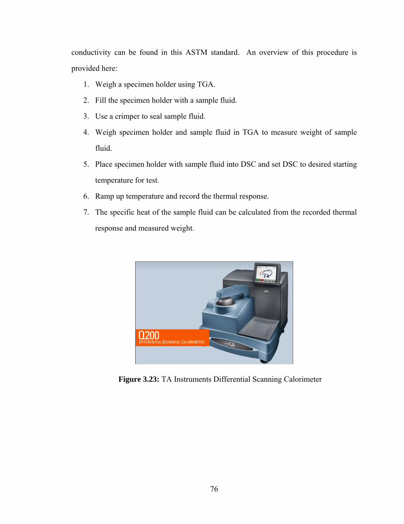
76
conductivity can be found in this ASTM standard. An overview of this procedure is
provided here:
1. Weigh a specimen holder using TGA.
2. Fill the specimen holder with a sample fluid.
3. Use a crimper to seal sample fluid.
4. Weigh specimen holder and sample fluid in TGA to measure weight of sample
fluid.
5. Place specimen holder with sample fluid into DSC and set DSC to desired starting
temperature for test.
6. Ramp up temperature and record the thermal response.
7. The specific heat of the sample fluid can be calculated from the recorded thermal
response and measured weight.
Figure 3.23: TA Instruments Differential Scanning Calorimeter

77
P (atm) T (K) CP (J/g-K) 1.00 320 1.782 1.00 325 1.812 1.00 330 1.817 1.00 335 1.819 1.00 340 1.820 1.00 345 1.823 1.00 350 1.823 1.00 355 1.825 1.00 360 1.825 1.00 365 1.825 1.00 370 1.830 1.00 375 1.850
Figure 3.24: TA Instruments Thermogravimetric Analyzer
Table 3.9: Measured Specific Heat of DMAZ (CP)

78
An application of the thermophysical property calculation method described in
this work was performed for two different HEDM compounds: Quadricyclane and
DMAZ. A model compound is identified for each HEDM compound and utilized in the
thermophysical property calculation method to determine the appropriate values for the
intermolecular parameters of the COMPASS model to be used for the corresponding
HEDM compound. This is done due to the fact that there is generally limited
experimental data for HEDM compounds, but more extensive data for their
corresponding model compounds. Model compounds are chosen based upon their having
a similar molecular structure to their corresponding HEDM compounds.
4.1 MODEL COMPOUNDS: NORBORNANE AND ETHYL AZIDE
The first step in calculating the thermophysical properties of DMAZ and
quadricyclane is to select a model compound for each HEDM compound. The rules
defined in Section 3.3 are used to select the appropriate model compounds. These rules
are repeated here:
Rule 1: The model compound must have a “similar” molecular structure as
the corresponding HEDM compound.
For DMAZ, this rule means that the model compound must have an azide chain
(near linear chain of three nitrogen atoms). For quadricyclane, this rule means that the
model compound must be a bicyclic compound (a molecule with two fused rings).
CHAPTER 4
FINAL APPLICATION

79
Rule 2: The model compound must have the same atom types as the HEDM
compound.
For DMAZ, this means that the molecule must have the three nitrogen atom types
in the azide chain, a carbon atom type attached to the end of the azide chain, and a
nonpolar hydrogen atom type. For quadricyclane, this means that the molecule must have
two carbon atom types: one with two heavy atoms attached and one with three heavy
atoms attached. The molecule must also have a nonpolar hydrogen atom type.
Rule 3: The model compound must have some density and enthalpy (or
specific heat) experimental data in the liquid phase.
The model compound that meets the requirements of the first two rules must also
have some density and enthalpy or specific heat experimental data. Extensive
experimental data is preferable, but will often times not exist due to the potentially strict
requirements set forth in rules 1 and 2.
Using these three rules, the model compounds chosen for DMAZ and
quadricyclane are ethyl azide and norbornane respectively. Figure 4.1 provides ball and
cylinder renderings of ethyl azide and DMAZ. As can be seen from the ball and cylinder
renderings, ethyl azide has the same azide chain found in DMAZ. Ethyl azide also has
the same three nitrogen atom types and the same carbon atom type attached to the end of
the azide chain. Ethyl azide also has a nonpolar hydrogen atom type like DMAZ. The
standard carbons and nitrogen found on the right side of the DMAZ molecule in Figure
4.1 were not required in the model compound, because their intermolecular parameters
are well defined in the COMPASS model (the baseline COMPASS values for these atom
types were used in the modeling of DMAZ) and they do not play a significant role in the

80
prediction of density. The outer atoms of the molecule are most important in the
prediction of the liquid density of a substance [59].
Figure 4.2 provides ball and cylinder renderings for norbornane and
quadricyclane. Norbornane is a bicyclic compound with the top three carbon atoms in
Figure 4.2a belonging to two different five-carbon rings. Like quadricyclane, norbornane
has two different carbon atom types: a carbon attached to two heavy atoms (the top
carbon atom and bottom four carbon atoms in Figure 4.2a are this atom type) and a
carbon atom attached to three heavy atoms (the middle two carbon atoms are this atom
type). Norbornane also has the same nonpolar hydrogen atom type as quadricyclane.
Figure 4.1: Ball and Cylinder Renderings of (a) Ethyl Azide and (b) DMAZ
Figure 4.2: Ball and Cylinder Renderings of (a) Norbornane and (b) Quadricyclane
(a) (b)
(a) (b)
81
4.1.1 QUANTUM MECHANICS
With the model compounds ethyl azide and norbornane chosen, quantum
mechanical techniques are performed for two main purposes:
1. Find the minimum energy configuration of each model compound in order
to perform vibrational normal mode quantum mechanical analyses and
molecular dynamics simulations.
2. Calculate the normal mode vibrational frequencies in order to calculate the
ideal gas sensible enthalpy.
Determination of Minimum Energy Configuration
The minimum energy configuration of each model compound is determined using
the GAMESS quantum mechanical software. An initial molecular configuration (initial
guess) is needed as input to GAMESS to start the optimization process. These initial
molecular configurations are provided to GAMESS from a molecular dynamics
conformational analysis performed using the LAMMPS molecular dynamics software
[38]. Table 4.1 and Table 4.2 provide the results of the LAMMPS conformational search
and GAMESS optimization for norbornane and ethyl azide respectively. As can be seen
in Table 4.1, the LAMMPS conformational search provides a very good starting point for
the norbornane geometry and only a small refinement by GAMESS is required. For ethyl
azide (Table 4.2), the LAMMPS conformational provides a poorer starting point that
requires more refinement from the GAMESS optimizer.
The minimum energy configurations found by GAMESS are used for quantum
mechanical vibrational analyses and for molecular dynamics simulations. As discussed
in section 3.2.1, a DFT energy calculation method with the B3LYP functional and the 6-
31G* basis set is used for all GAMESS energy calculations.

82
Conformational Search Results GAMESS Results Atom X (Ǻ) Y (Ǻ) Z (Ǻ) X (Ǻ) Y (Ǻ) Z (Ǻ)
C -0.194 0.078 2.109 -0.192 0.079 2.097 C -0.064 -1.061 1.065 -0.063 -1.058 1.059 C 0.081 1.208 1.083 0.084 1.205 1.075 C -1.094 -0.619 0.006 -1.109 -0.630 0.001 C 1.336 -0.780 0.486 1.351 -0.794 0.487 C 1.433 0.758 0.492 1.450 0.769 0.493 C -0.998 0.919 0.020 -1.012 0.933 0.016 H 0.575 0.023 2.909 0.558 0.025 2.897 H -1.206 0.140 2.561 -1.188 0.143 2.552 H -0.208 -2.090 1.444 -0.205 -2.076 1.437 H 0.073 2.241 1.479 0.075 2.227 1.468 H -2.119 -0.958 0.290 -2.113 -0.968 0.285 H -1.971 1.378 0.316 -1.965 1.382 0.319 H -0.852 -1.037 -0.999 -0.893 -1.057 -0.986 H -0.708 1.323 -0.977 -0.752 1.351 -0.963 H 1.445 -1.195 -0.542 1.475 -1.220 -0.515 H 2.125 -1.232 1.134 2.121 -1.240 1.128 H 2.277 1.104 1.136 2.272 1.110 1.133 H 1.585 1.164 -0.535 1.622 1.184 -0.506
Conformational Search Results GAMESS Results Atom X (Ǻ) Y (Ǻ) Z (Ǻ) X (Ǻ) Y (Ǻ) Z (Ǻ)
N -1.603 0.630 -3.827 -1.229 0.511 -3.933 N -1.258 -0.208 -3.156 -1.177 -0.275 -3.160 N -1.092 -1.231 -2.436 -1.215 -1.160 -2.311 C 0.199 -1.558 -1.811 0.112 -1.540 -1.797 C 0.697 -0.530 -0.793 0.661 -0.541 -0.785 H 0.987 -1.753 -2.577 0.813 -1.678 -2.616 H -0.027 -2.518 -1.313 -0.035 -2.503 -1.331 H 1.441 -1.014 -0.123 1.610 -0.889 -0.389 H -0.127 -0.184 -0.136 -0.031 -0.416 0.039 H 1.117 0.307 -1.35 0.826 0.432 -1.240
Calculation of Ideal Gas Sensible Enthalpy
With the minimum energy configurations of norbornane and ethyl azide
determined, a normal mode vibrational analysis can be performed using GAMESS in
order to calculate the normal mode vibrational frequencies. These vibrational frequencies
Table 4.1: Atomic Coordinates for Optimized Norbornane Geometry
Table 4.2: Atomic Coordinates for Optimized Ethyl Azide Geometry

83
are needed in order to calculate the ideal gas component of sensible enthalpy. Table 4.3
and Table 4.4 provide the results of the GAMESS normal mode vibrational analysis of
norbornane and ethyl azide respectively. There are 3N-6 vibrational modes in a non-
linear molecule where N is the number of atoms in the molecule. For norbornane this
translates into 51 vibrational modes (3*19-6=51), and for ethyl azide this translates into
24 vibrational modes (3*10-6=24). The 6 degrees of freedom subtracted from the 3N are
the 3 translational and 3 rotational (2 for a linear molecule) degrees of freedom. The
wave number (second column in both Table 4.3 and Table 4.4) is the value calculated and
outputted by GAMESS. The wave number is related to the vibrational frequency and
characteristic vibrational temperature with the following equations:
(68)
(69)
In the above equations, ν is the vibrational frequency, c is the speed of light in a
vacuum, k is the wave number, θvib is the characteristic vibrational temperature, h is
Planck’s constant, and kB is Boltzmann’s constant. The vibrational contribution to the
specific heat at constant volume from a particular vibrational mode is calculated with the
following equation:
(70)
where R is the universal gas constant and T is the temperature.
ck=ν
Bvib k
hνθ =
( )2
2
1−⎟⎠⎞
⎜⎝⎛=
T/
T/vibvib
Vvib
vib
e
eT
R)T(Cθ
θθ

84
Mode Wave #, k (1/cm) θvib (K) CVvib – 298.15 K (J/mol-K)
1 151 217 7.9562 2 330 475 6.7600 3 400 576 6.1473 4 461 663 5.5927 5 546 786 4.8051 6 761 1095 3.0019 7 764 1100 2.9752 8 810 1165 2.6540 9 822 1183 2.5718
10 825 1187 2.5543 11 887 1277 2.1647 12 899 1294 2.0951 13 930 1338 1.9244 14 959 1380 1.7759 15 967 1391 1.7356 16 971 1397 1.7151 17 975 1403 1.6941 18 1008 1450 1.5417 19 1048 1508 1.3704 20 1102 1586 1.1639 21 1135 1633 1.0521 22 1148 1652 1.0103 23 1173 1688 0.9333 24 1195 1720 0.8696 25 1245 1791 0.7415 26 1248 1796 0.7338 27 1282 1845 0.6564 28 1294 1862 0.6322 29 1302 1873 0.6163 30 1316 1894 0.5867 31 1341 1929 0.5403 32 1354 1948 0.5173 33 1363 1960 0.5026 34 1367 1967 0.4953 35 1508 2169 0.3051 36 1522 2189 0.2905 37 1528 2199 0.2839 38 1530 2202 0.2818 39 1556 2239 0.2571 40 3041 4376 0.0008 41 3047 4384 0.0007 42 3054 4394 0.0007 43 3057 4398 0.0007 44 3068 4415 0.0007 45 3081 4432 0.0006 46 3086 4440 0.0006 47 3092 4448 0.0006 48 3096 4455 0.0006 49 3105 4468 0.0006 50 3110 4475 0.0006 51 3113 4480 0.0006
Table 4.3: Normal Mode Vibrational Frequencies of Norbornane

85
Mode Wave #, k (1/cm) θvib (K) CVvib – 298.15 K (J/mol-K)
1 67 96 8.2430 2 196 283 7.7191 3 287 414 7.1004 4 400 576 6.1476 5 574 826 4.5501 6 662 952 3.7822 7 809 1165 2.6576 8 855 1230 2.3632 9 1003 1442 1.5666
10 1105 1591 1.1519 11 1168 1681 0.9472 12 1300 1870 0.6196 13 1342 1931 0.5385 14 1397 2011 0.4466 15 1441 2073 0.3850 16 1518 2184 0.2943 17 1522 2189 0.2904 18 1534 2207 0.2782 19 2252 3240 0.0187 20 3038 4371 0.0008 21 3040 4374 0.0008 22 3102 4463 0.0006 23 3122 4491 0.0005 24 3143 4522 0.0005
The total specific heat at constant volume of a molecule is the sum of each of
these vibrational contributions, the translational contribution, and the rotational
contribution. This equation for a non-linear molecule is provided below:
(71)
Table 4.5 and Table 4.6 provide the results of this calculation of the ideal gas
specific heat and sensible enthalpy as a function of temperature for norbornane and ethyl
azide respectively. The equation used to calculate the ideal gas sensible enthalpy (less
RT) is provided below:
(72)
Table 4.4: Normal Mode Vibrational Frequencies of Ethyl Azide
( )∑−
= −⎟⎟⎠
⎞⎜⎜⎝
⎛++=++=−=
63
12
2
23
23
1
N
iT/
T/vibvib
VrotV
trV
igP
igV
ivib
ivibi
e
eT
RRRCCCR)T(C)T(Cθ
θθ
∫=−T
K.
igV
igsens d)(CRTh
15298
ττ

86
Temperature (K)
CV_trans (J/mol-K)
CV_rot (J/mol-K)
CV_vib (J/mol-K)
CV (J/mol-K)
RThigsens − (kJ/mol)
298.15 12.4715 12.4715 73.5130 98.4563 0.0000 360.00 12.4715 12.4715 102.7500 127.6934 6.9937 365.00 12.4715 12.4715 105.1030 130.0463 7.6380 370.00 12.4715 12.4715 107.4480 132.3913 8.2941 375.00 12.4715 12.4715 109.7840 134.7274 8.9619 380.00 12.4715 12.4715 112.1110 137.0535 9.6414
Temperature (K)
CV_trans (J/mol-K)
CV_rot (J/mol-K)
CV_vib (J/mol-K)
CV (J/mol-K)
RThigsens − (kJ/mol)
273.15 12.4715 12.4715 44.5560 69.4987 -1.7942 283.15 12.4715 12.4715 46.3670 71.3100 -1.0902 293.15 12.4715 12.4715 48.1890 73.1321 -0.3679 298.15 12.4715 12.4715 49.1030 74.0464 0.0000 303.15 12.4715 12.4715 50.0190 74.9624 0.3725 313.15 12.4715 12.4715 51.8550 76.7980 1.1313 323.15 12.4715 12.4715 53.6930 78.6362 1.9085
4.1.2 MOLECULAR DYNAMICS
With the ideal gas sensible enthalpy calculated, molecular dynamics simulations
of the model compounds can be performed to determine the optimal values for the
intermolecular parameters of the COMPASS model (σ and ε in the last term of equation
(2)) for each atom type to most closely match experimental density and enthalpy data.
Design of Experiments
The creation of a DOE of molecular dynamics runs is performed with the goal of
creating a response surface equation to approximate the design space. The design space
being explored is of the density and specific heat as a function of the intermolecular
parameter multipliers. Table 4.11 and Table 4.12 are the DOE’s of molecular dynamics
Table 4.5: Ideal Gas Sensible Enthalpy Results for Norbornane
Table 4.6: Ideal Gas Sensible Enthalpy Results for Ethyl Azide

87
runs for norbornane and ethyl azide respectively in order to determine the sensitivity of
density to changes in the intermolecular parameters. The multiplier values in these tables
are multipliers of the baseline COMPASS intermolecular parameter values for each atom
type of interest. These DOE run tables are created using the JMP Statistical Discovery
software tool [57]. The baseline values are provided in Table 4.7 and Table 4.8 for
norbornane and ethyl azide respectively.
σc4 εc4 σc43 εc43 σh1 εh1 3.854 0.062 3.854 0.040 2.878 0.023
σn1z εn1z σn2t εn2t σn2z εn2z σc4z εc4z σh1 εh1 3.520 0.085 3.300 0.050 3.400 0.120 3.650 0.080 2.878 0.023
Table 4.9 and Table 4.10 provide the baseline COMPASS model charge bond
increments for each bond type for norbornane and ethyl azide respectively. The charge
bond increments are used to compute the charge associated with each atom in a molecule.
δc4-c43 δc4-c4 δc4-h1 δc43-h1 0.0000 0.0000 -0.0530 -0.0530
δn1z-n2t δn2t-n2z δn2z-c4z δc4z-c4 δc4z-h1 δc4-h1 -0.3860 0.2470 -0.3110 0.0000 -0.0530 -0.0530
Table 4.7: Norbornane Baseline COMPASS Intermolecular Parameter Values
Table 4.8: Ethyl Azide Baseline COMPASS Intermolecular Parameter Values
Table 4.9: Norbornane Baseline COMPASS Charge Bond Increments
Table 4.10: Ethyl Azide Baseline COMPASS Charge Bond Increments

88
Equation (73) describes how the charge associated with each atom is calculated
from the charge bond increments. In equation (73), the charge for the ith atom in the
molecule is calculated by summing the charge bond increments for the n atoms bonded to
atom i. For this research work, the charge bond increments were not adjusted in the
intermolecular parameter optimization process. Discussion on the potential benefits of
adjusting these parameters is provided in Chapter 6.
(73)
All runs in a particular DOE for density are performed at the same temperature
and pressure: 360 K and 1 atm for norbornane and 298.15 K and 1 atm for ethyl azide.
This is done because experimental density data exists for liquid norbornane and liquid
ethyl azide respectively at these temperatures and pressures.
∑=
=n
jijiq
1
δ
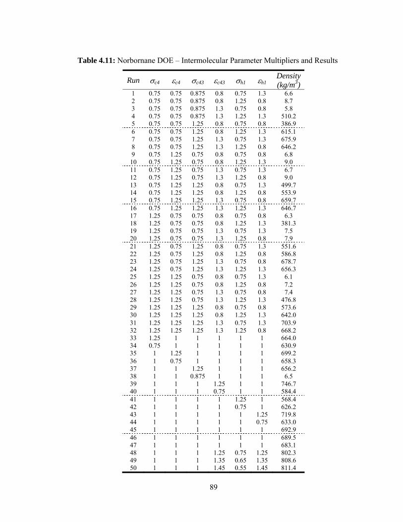
89
Run σc4 εc4 σc43 εc43 σh1 εh1 Density (kg/m3)
1 0.75 0.75 0.875 0.8 0.75 1.3 6.6 2 0.75 0.75 0.875 0.8 1.25 0.8 8.7 3 0.75 0.75 0.875 1.3 0.75 0.8 5.8 4 0.75 0.75 0.875 1.3 1.25 1.3 510.2 5 0.75 0.75 1.25 0.8 0.75 0.8 386.9 6 0.75 0.75 1.25 0.8 1.25 1.3 615.1 7 0.75 0.75 1.25 1.3 0.75 1.3 675.9 8 0.75 0.75 1.25 1.3 1.25 0.8 646.2 9 0.75 1.25 0.75 0.8 0.75 0.8 6.8
10 0.75 1.25 0.75 0.8 1.25 1.3 9.0 11 0.75 1.25 0.75 1.3 0.75 1.3 6.7 12 0.75 1.25 0.75 1.3 1.25 0.8 9.0 13 0.75 1.25 1.25 0.8 0.75 1.3 499.7 14 0.75 1.25 1.25 0.8 1.25 0.8 553.9 15 0.75 1.25 1.25 1.3 0.75 0.8 659.7 16 0.75 1.25 1.25 1.3 1.25 1.3 646.7 17 1.25 0.75 0.75 0.8 0.75 0.8 6.3 18 1.25 0.75 0.75 0.8 1.25 1.3 381.3 19 1.25 0.75 0.75 1.3 0.75 1.3 7.5 20 1.25 0.75 0.75 1.3 1.25 0.8 7.9 21 1.25 0.75 1.25 0.8 0.75 1.3 551.6 22 1.25 0.75 1.25 0.8 1.25 0.8 586.8 23 1.25 0.75 1.25 1.3 0.75 0.8 678.7 24 1.25 0.75 1.25 1.3 1.25 1.3 656.3 25 1.25 1.25 0.75 0.8 0.75 1.3 6.1 26 1.25 1.25 0.75 0.8 1.25 0.8 7.2 27 1.25 1.25 0.75 1.3 0.75 0.8 7.4 28 1.25 1.25 0.75 1.3 1.25 1.3 476.8 29 1.25 1.25 1.25 0.8 0.75 0.8 573.6 30 1.25 1.25 1.25 0.8 1.25 1.3 642.0 31 1.25 1.25 1.25 1.3 0.75 1.3 703.9 32 1.25 1.25 1.25 1.3 1.25 0.8 668.2 33 1.25 1 1 1 1 1 664.0 34 0.75 1 1 1 1 1 630.9 35 1 1.25 1 1 1 1 699.2 36 1 0.75 1 1 1 1 658.3 37 1 1 1.25 1 1 1 656.2 38 1 1 0.875 1 1 1 6.5 39 1 1 1 1.25 1 1 746.7 40 1 1 1 0.75 1 1 584.4 41 1 1 1 1 1.25 1 568.4 42 1 1 1 1 0.75 1 626.2 43 1 1 1 1 1 1.25 719.8 44 1 1 1 1 1 0.75 633.0 45 1 1 1 1 1 1 692.9 46 1 1 1 1 1 1 689.5 47 1 1 1 1 1 1 683.1 48 1 1 1 1.25 0.75 1.25 802.3 49 1 1 1 1.35 0.65 1.35 808.6 50 1 1 1 1.45 0.55 1.45 811.4
Table 4.11: Norbornane DOE – Intermolecular Parameter Multipliers and Results

90
Run σn1z εn1z σn2t εn2t σn2z εn2z σc4z εc4z σh1 εh1 Density (kg/m3)
1 0.8 0.8 0.8 0.8 0.8 0.8 0.8 0.8 1.2 1.2 762.3 2 0.8 0.8 0.8 0.8 0.8 0.8 1.2 1.2 1.2 0.8 799.1 3 0.8 0.8 0.8 0.8 0.8 1.2 0.8 1.2 0.8 1.2 1182.1 4 0.8 0.8 0.8 0.8 0.8 1.2 1.2 0.8 0.8 0.8 915.2 5 0.8 0.8 0.8 0.8 1.2 0.8 0.8 1.2 0.8 0.8 836.4 6 0.8 0.8 0.8 0.8 1.2 0.8 1.2 0.8 0.8 1.2 852.3 7 0.8 0.8 0.8 0.8 1.2 1.2 0.8 0.8 1.2 0.8 688.5 8 0.8 0.8 0.8 0.8 1.2 1.2 1.2 1.2 1.2 1.2 821.8 9 0.8 0.8 0.8 1.2 0.8 0.8 0.8 1.2 0.8 0.8 1127.8
10 0.8 0.8 0.8 1.2 0.8 0.8 1.2 0.8 0.8 1.2 966.3 11 0.8 0.8 0.8 1.2 0.8 1.2 0.8 0.8 1.2 0.8 713.8 12 0.8 0.8 0.8 1.2 0.8 1.2 1.2 1.2 1.2 1.2 863.1 13 0.8 0.8 0.8 1.2 1.2 0.8 0.8 0.8 1.2 1.2 720.0 14 0.8 0.8 0.8 1.2 1.2 0.8 1.2 1.2 1.2 0.8 778.5 15 0.8 0.8 0.8 1.2 1.2 1.2 0.8 1.2 0.8 1.2 909.9 16 0.8 0.8 0.8 1.2 1.2 1.2 1.2 0.8 0.8 0.8 871.5 17 0.8 0.8 1.2 0.8 0.8 0.8 0.8 1.2 0.8 0.8 870.5 18 0.8 0.8 1.2 0.8 0.8 0.8 1.2 0.8 0.8 1.2 845.2 19 0.8 0.8 1.2 0.8 0.8 1.2 0.8 0.8 1.2 0.8 661.5 20 0.8 0.8 1.2 0.8 0.8 1.2 1.2 1.2 1.2 1.2 805.6 21 0.8 0.8 1.2 0.8 1.2 0.8 0.8 0.8 1.2 1.2 714.6 22 0.8 0.8 1.2 0.8 1.2 0.8 1.2 1.2 1.2 0.8 781.4 23 0.8 0.8 1.2 0.8 1.2 1.2 0.8 1.2 0.8 1.2 885.0 24 0.8 0.8 1.2 0.8 1.2 1.2 1.2 0.8 0.8 0.8 872.0 25 0.8 0.8 1.2 1.2 0.8 0.8 0.8 0.8 1.2 1.2 704.7 26 0.8 0.8 1.2 1.2 0.8 0.8 1.2 1.2 1.2 0.8 781.7 27 0.8 0.8 1.2 1.2 0.8 1.2 0.8 1.2 0.8 1.2 958.4 28 0.8 0.8 1.2 1.2 0.8 1.2 1.2 0.8 0.8 0.8 860.6 29 0.8 0.8 1.2 1.2 1.2 0.8 0.8 1.2 0.8 0.8 856.8 30 0.8 0.8 1.2 1.2 1.2 0.8 1.2 0.8 0.8 1.2 877.5 31 0.8 0.8 1.2 1.2 1.2 1.2 0.8 0.8 1.2 0.8 728.3 32 0.8 0.8 1.2 1.2 1.2 1.2 1.2 1.2 1.2 1.2 826.2 33 0.8 1.2 0.8 0.8 0.8 0.8 0.8 1.2 0.8 0.8 1125.0 34 0.8 1.2 0.8 0.8 0.8 0.8 1.2 0.8 0.8 1.2 988.4 35 0.8 1.2 0.8 0.8 0.8 1.2 0.8 0.8 1.2 0.8 717.8 36 0.8 1.2 0.8 0.8 0.8 1.2 1.2 1.2 1.2 1.2 869.9 37 0.8 1.2 0.8 0.8 1.2 0.8 0.8 0.8 1.2 1.2 717.6 38 0.8 1.2 0.8 0.8 1.2 0.8 1.2 1.2 1.2 0.8 790.6 39 0.8 1.2 0.8 0.8 1.2 1.2 0.8 1.2 0.8 1.2 910.7 40 0.8 1.2 0.8 0.8 1.2 1.2 1.2 0.8 0.8 0.8 863.0 41 0.8 1.2 0.8 1.2 0.8 0.8 0.8 0.8 1.2 1.2 778.4 42 0.8 1.2 0.8 1.2 0.8 0.8 1.2 1.2 1.2 0.8 836.2 43 0.8 1.2 0.8 1.2 0.8 1.2 0.8 1.2 0.8 1.2 1186.4 44 0.8 1.2 0.8 1.2 0.8 1.2 1.2 0.8 0.8 0.8 968.0 45 0.8 1.2 0.8 1.2 1.2 0.8 0.8 1.2 0.8 0.8 850.6 46 0.8 1.2 0.8 1.2 1.2 0.8 1.2 0.8 0.8 1.2 853.6 47 0.8 1.2 0.8 1.2 1.2 1.2 0.8 0.8 1.2 0.8 704.7 48 0.8 1.2 0.8 1.2 1.2 1.2 1.2 1.2 1.2 1.2 834.4 49 0.8 1.2 1.2 0.8 0.8 0.8 0.8 0.8 1.2 1.2 703.5 50 0.8 1.2 1.2 0.8 0.8 0.8 1.2 1.2 1.2 0.8 773.9
Table 4.12: Ethyl Azide DOE – Intermolecular Parameter Multipliers and Density

91
51 0.8 1.2 1.2 0.8 0.8 1.2 0.8 1.2 0.8 1.2 969.6 52 0.8 1.2 1.2 0.8 0.8 1.2 1.2 0.8 0.8 0.8 851.7 53 0.8 1.2 1.2 0.8 1.2 0.8 0.8 1.2 0.8 0.8 843.8 54 0.8 1.2 1.2 0.8 1.2 0.8 1.2 0.8 0.8 1.2 839.8 55 0.8 1.2 1.2 0.8 1.2 1.2 0.8 0.8 1.2 0.8 724.5 56 0.8 1.2 1.2 0.8 1.2 1.2 1.2 1.2 1.2 1.2 821.9 57 0.8 1.2 1.2 1.2 0.8 0.8 0.8 1.2 0.8 0.8 925.7 58 0.8 1.2 1.2 1.2 0.8 0.8 1.2 0.8 0.8 1.2 881.0 59 0.8 1.2 1.2 1.2 0.8 1.2 0.8 0.8 1.2 0.8 685.2 60 0.8 1.2 1.2 1.2 0.8 1.2 1.2 1.2 1.2 1.2 824.2 61 0.8 1.2 1.2 1.2 1.2 0.8 0.8 0.8 1.2 1.2 729.9 62 0.8 1.2 1.2 1.2 1.2 0.8 1.2 1.2 1.2 0.8 798.8 63 0.8 1.2 1.2 1.2 1.2 1.2 0.8 1.2 0.8 1.2 917.8 64 0.8 1.2 1.2 1.2 1.2 1.2 1.2 0.8 0.8 0.8 894.3 65 1.2 0.8 0.8 0.8 0.8 0.8 0.8 1.2 0.8 0.8 344.5 66 1.2 0.8 0.8 0.8 0.8 0.8 1.2 0.8 0.8 1.2 589.2 67 1.2 0.8 0.8 0.8 0.8 1.2 0.8 0.8 1.2 0.8 428.8 68 1.2 0.8 0.8 0.8 0.8 1.2 1.2 1.2 1.2 1.2 660.2 69 1.2 0.8 0.8 0.8 1.2 0.8 0.8 0.8 1.2 1.2 568.8 70 1.2 0.8 0.8 0.8 1.2 0.8 1.2 1.2 1.2 0.8 643.7 71 1.2 0.8 0.8 0.8 1.2 1.2 0.8 1.2 0.8 1.2 628.1 72 1.2 0.8 0.8 0.8 1.2 1.2 1.2 0.8 0.8 0.8 667.4 73 1.2 0.8 0.8 1.2 0.8 0.8 0.8 0.8 1.2 1.2 520.2 74 1.2 0.8 0.8 1.2 0.8 0.8 1.2 1.2 1.2 0.8 622.3 75 1.2 0.8 0.8 1.2 0.8 1.2 0.8 1.2 0.8 1.2 638.9 76 1.2 0.8 0.8 1.2 0.8 1.2 1.2 0.8 0.8 0.8 552.7 77 1.2 0.8 0.8 1.2 1.2 0.8 0.8 1.2 0.8 0.8 523.6 78 1.2 0.8 0.8 1.2 1.2 0.8 1.2 0.8 0.8 1.2 635.6 79 1.2 0.8 0.8 1.2 1.2 1.2 0.8 0.8 1.2 0.8 550.4 80 1.2 0.8 0.8 1.2 1.2 1.2 1.2 1.2 1.2 1.2 688.1 81 1.2 0.8 1.2 0.8 0.8 0.8 0.8 0.8 1.2 1.2 586.7 82 1.2 0.8 1.2 0.8 0.8 0.8 1.2 1.2 1.2 0.8 656.9 83 1.2 0.8 1.2 0.8 0.8 1.2 0.8 1.2 0.8 1.2 660.7 84 1.2 0.8 1.2 0.8 0.8 1.2 1.2 0.8 0.8 0.8 660.0 85 1.2 0.8 1.2 0.8 1.2 0.8 0.8 1.2 0.8 0.8 648.5 86 1.2 0.8 1.2 0.8 1.2 0.8 1.2 0.8 0.8 1.2 711.8 87 1.2 0.8 1.2 0.8 1.2 1.2 0.8 0.8 1.2 0.8 615.0 88 1.2 0.8 1.2 0.8 1.2 1.2 1.2 1.2 1.2 1.2 717.2 89 1.2 0.8 1.2 1.2 0.8 0.8 0.8 1.2 0.8 0.8 662.8 90 1.2 0.8 1.2 1.2 0.8 0.8 1.2 0.8 0.8 1.2 685.4 91 1.2 0.8 1.2 1.2 0.8 1.2 0.8 0.8 1.2 0.8 581.3 92 1.2 0.8 1.2 1.2 0.8 1.2 1.2 1.2 1.2 1.2 693.7 93 1.2 0.8 1.2 1.2 1.2 0.8 0.8 0.8 1.2 1.2 638.7 94 1.2 0.8 1.2 1.2 1.2 0.8 1.2 1.2 1.2 0.8 697.7 95 1.2 0.8 1.2 1.2 1.2 1.2 0.8 1.2 0.8 1.2 733.9 96 1.2 0.8 1.2 1.2 1.2 1.2 1.2 0.8 0.8 0.8 745.9 97 1.2 1.2 0.8 0.8 0.8 0.8 0.8 0.8 1.2 1.2 545.4 98 1.2 1.2 0.8 0.8 0.8 0.8 1.2 1.2 1.2 0.8 632.1 99 1.2 1.2 0.8 0.8 0.8 1.2 0.8 1.2 0.8 1.2 646.7
100 1.2 1.2 0.8 0.8 0.8 1.2 1.2 0.8 0.8 0.8 611.0 101 1.2 1.2 0.8 0.8 1.2 0.8 0.8 1.2 0.8 0.8 522.1 102 1.2 1.2 0.8 0.8 1.2 0.8 1.2 0.8 0.8 1.2 647.0 103 1.2 1.2 0.8 0.8 1.2 1.2 0.8 0.8 1.2 0.8 587.9 104 1.2 1.2 0.8 0.8 1.2 1.2 1.2 1.2 1.2 1.2 688.6
Table 4.12 (continued)

92
105 1.2 1.2 0.8 1.2 0.8 0.8 0.8 1.2 0.8 0.8 572.2 106 1.2 1.2 0.8 1.2 0.8 0.8 1.2 0.8 0.8 1.2 665.9 107 1.2 1.2 0.8 1.2 0.8 1.2 0.8 0.8 1.2 0.8 517.0 108 1.2 1.2 0.8 1.2 0.8 1.2 1.2 1.2 1.2 1.2 688.4 109 1.2 1.2 0.8 1.2 1.2 0.8 0.8 0.8 1.2 1.2 582.3 110 1.2 1.2 0.8 1.2 1.2 0.8 1.2 1.2 1.2 0.8 663.1 111 1.2 1.2 0.8 1.2 1.2 1.2 0.8 1.2 0.8 1.2 647.5 112 1.2 1.2 0.8 1.2 1.2 1.2 1.2 0.8 0.8 0.8 695.6 113 1.2 1.2 1.2 0.8 0.8 0.8 0.8 1.2 0.8 0.8 657.6 114 1.2 1.2 1.2 0.8 0.8 0.8 1.2 0.8 0.8 1.2 694.9 115 1.2 1.2 1.2 0.8 0.8 1.2 0.8 0.8 1.2 0.8 581.3 116 1.2 1.2 1.2 0.8 0.8 1.2 1.2 1.2 1.2 1.2 699.9 117 1.2 1.2 1.2 0.8 1.2 0.8 0.8 0.8 1.2 1.2 622.8 118 1.2 1.2 1.2 0.8 1.2 0.8 1.2 1.2 1.2 0.8 692.6 119 1.2 1.2 1.2 0.8 1.2 1.2 0.8 1.2 0.8 1.2 726.4 120 1.2 1.2 1.2 0.8 1.2 1.2 1.2 0.8 0.8 0.8 742.1 121 1.2 1.2 1.2 1.2 0.8 0.8 0.8 0.8 1.2 1.2 608.0 122 1.2 1.2 1.2 1.2 0.8 0.8 1.2 1.2 1.2 0.8 686.5 123 1.2 1.2 1.2 1.2 0.8 1.2 0.8 1.2 0.8 1.2 736.9 124 1.2 1.2 1.2 1.2 0.8 1.2 1.2 0.8 0.8 0.8 742.0 125 1.2 1.2 1.2 1.2 1.2 0.8 0.8 1.2 0.8 0.8 703.5 126 1.2 1.2 1.2 1.2 1.2 0.8 1.2 0.8 0.8 1.2 739.9 127 1.2 1.2 1.2 1.2 1.2 1.2 0.8 0.8 1.2 0.8 643.5 128 1.2 1.2 1.2 1.2 1.2 1.2 1.2 1.2 1.2 1.2 733.8 129 0.8 1 1 1 1 1 1 1 1 1 988.0 130 1.2 1 1 1 1 1 1 1 1 1 728.8 131 1 0.8 1 1 1 1 1 1 1 1 875.8 132 1 1.2 1 1 1 1 1 1 1 1 900.3 133 1 1 0.8 1 1 1 1 1 1 1 874.6 134 1 1 1.2 1 1 1 1 1 1 1 870.0 135 1 1 1 0.8 1 1 1 1 1 1 882.1 136 1 1 1 1.2 1 1 1 1 1 1 910.2 137 1 1 1 1 0.8 1 1 1 1 1 891.0 138 1 1 1 1 1.2 1 1 1 1 1 840.6 139 1 1 1 1 1 0.8 1 1 1 1 883.5 140 1 1 1 1 1 1.2 1 1 1 1 909.9 141 1 1 1 1 1 1 0.8 1 1 1 845.5 142 1 1 1 1 1 1 1.2 1 1 1 868.5 143 1 1 1 1 1 1 1 0.8 1 1 871.7 144 1 1 1 1 1 1 1 1.2 1 1 907.2 145 1 1 1 1 1 1 1 1 0.8 1 929.2 146 1 1 1 1 1 1 1 1 1.2 1 782.6 147 1 1 1 1 1 1 1 1 1 0.8 886.1 148 1 1 1 1 1 1 1 1 1 1.2 898.6 149 1 1 1 1 1 1 1 1 1 1 891.7 150 1 1 1 1 1 1 1 1 1 1 885.7 151 1 1 1 1 1 1 1 1 1 1 901.4
Table 4.12 (continued)

93
In addition to the above DOE’s used to determine the sensitivity of density to
changes in intermolecular parameters, the DOE’s in Table 4.13 and Table 4.14 are used
to determine the sensitivity of specific heat to changes in intermolecular parameters.
These DOE’s are different from the density DOE’s because for a particular set of
intermolecular parameter settings, two runs are performed at different temperatures in
order to calculate the change in enthalpy as a function of temperature (to compute
specific heat). For norbornane, molecular dynamics runs are performed at 360 K and 380
K, both at 1 atm. For ethyl azide, molecular dynamics runs are performed at 273.15 K
and 323.15 K, both at 1 atm. These temperatures and pressures are chosen because there
is experimental liquid data available.
The combination of the density and specific heat DOE’s are used to create
response surface equations to determine the optimal settings for the intermolecular
parameters. In Table 4.13 and Table 4.14, the specific heat is calculated using equations
(11) – (14). These equations are repeated here for convenience:
(74)
(75)
(76)
(77)
)P,T(CR)T(C)P,T(C resP
igPP +−=
( )∑−
= −⎟⎟⎠
⎞⎜⎜⎝
⎛++=++=−
63
12
2
23
23
1
N
iT/
T/vibvib
VrotV
trV
igP
ivib
ivibi
e
eT
RRRCCCR)T(Cθ
θθ
P
erint
P
resresP )P,T(
P)P,T(PETT
)P,T(H)P,T(C ⎟⎟
⎠
⎞⎜⎜⎝
⎛+
∂∂
=⎟⎟
⎠
⎞
⎜⎜
⎝
⎛
∂
∂=
ρ
∫ −=−T
K.
igP
igsens RTd)(CRTh
15298
ττ

94
Run Τ (Κ) σc4 εc4 σc43 εc43 σh1 εh1 CP
(cal/mol-K) 1 360 1.1 1 1 1 1 1 2 380 1.1 1 1 1 1 1 46.7537
3 360 0.9 1 1 1 1 1 4 380 0.9 1 1 1 1 1 48.6133
5 360 1 1.1 1 1 1 1 6 380 1 1.1 1 1 1 1 41.7002
7 360 1 0.9 1 1 1 1 8 380 1 0.9 1 1 1 1 48.9731
9 360 1 1 1.1 1 1 1 10 380 1 1 1.1 1 1 1 39.1577
11 360 1 1 0.9 1 1 1 12 380 1 1 0.9 1 1 1 50.6061
13 360 1 1 1 1.1 1 1 14 380 1 1 1 1.1 1 1 42.6354
15 360 1 1 1 0.9 1 1 16 380 1 1 1 0.9 1 1 51.7772
17 360 1 1 1 1 1.1 1 18 380 1 1 1 1 1.1 1 50.2793
19 360 1 1 1 1 0.9 1 20 380 1 1 1 1 0.9 1 40.2156
21 360 1 1 1 1 1 1.1 22 380 1 1 1 1 1 1.1 38.4435
23 360 1 1 1 1 1 0.9 24 380 1 1 1 1 1 0.9 48.0030
25 360 1 1 1 1 1 1 26 380 1 1 1 1 1 1 47.0211
Table 4.13: Norbornane DOE – Intermolecular Parameter Multipliers and CP

95
Run Τ (Κ) σn1z εn1z σn2t εn2t σn2z εn2z σc4z εc4z σh1 εh1 CP
(cal/mol-K)1 273.15 1.2 1 1 1 1 1 1 1 1 1 2 323.15 1.2 1 1 1 1 1 1 1 1 1 32.5021
3 273.15 0.8 1 1 1 1 1 1 1 1 1 4 323.15 0.8 1 1 1 1 1 1 1 1 1 36.4428
5 273.15 1 1.2 1 1 1 1 1 1 1 1 6 323.15 1 1.2 1 1 1 1 1 1 1 1 35.8510
7 273.15 1 0.8 1 1 1 1 1 1 1 1 8 323.15 1 0.8 1 1 1 1 1 1 1 1 36.1449
9 273.15 1 1 1.2 1 1 1 1 1 1 1 10 323.15 1 1 1.2 1 1 1 1 1 1 1 34.9052
11 273.15 1 1 0.8 1 1 1 1 1 1 1 12 323.15 1 1 0.8 1 1 1 1 1 1 1 34.1106
13 273.15 1 1 1 1.2 1 1 1 1 1 1 14 323.15 1 1 1 1.2 1 1 1 1 1 1 36.4420
15 273.15 1 1 1 0.8 1 1 1 1 1 1 16 323.15 1 1 1 0.8 1 1 1 1 1 1 32.3643
17 273.15 1 1 1 1 1.2 1 1 1 1 1 18 323.15 1 1 1 1 1.2 1 1 1 1 1 30.4584
19 273.15 1 1 1 1 0.8 1 1 1 1 1 20 323.15 1 1 1 1 0.8 1 1 1 1 1 38.0530
21 273.15 1 1 1 1 1 1.2 1 1 1 1 22 323.15 1 1 1 1 1 1.2 1 1 1 1 33.5489
23 273.15 1 1 1 1 1 0.8 1 1 1 1 24 323.15 1 1 1 1 1 0.8 1 1 1 1 35.6740
25 273.15 1 1 1 1 1 1 1.2 1 1 1 26 323.15 1 1 1 1 1 1 1.2 1 1 1 33.9286
27 273.15 1 1 1 1 1 1 0.8 1 1 1 28 323.15 1 1 1 1 1 1 0.8 1 1 1 36.0946
29 273.15 1 1 1 1 1 1 1 1.2 1 1 30 323.15 1 1 1 1 1 1 1 1.2 1 1 36.2093
31 273.15 1 1 1 1 1 1 1 0.8 1 1 32 323.15 1 1 1 1 1 1 1 0.8 1 1 35.4663
33 273.15 1 1 1 1 1 1 1 1 1.2 1 34 323.15 1 1 1 1 1 1 1 1 1.2 1 32.5348
35 273.15 1 1 1 1 1 1 1 1 0.8 1 36 323.15 1 1 1 1 1 1 1 1 0.8 1 37.5660
37 273.15 1 1 1 1 1 1 1 1 1 1.2 38 323.15 1 1 1 1 1 1 1 1 1 1.2 35.0169
39 273.15 1 1 1 1 1 1 1 1 1 0.8 40 323.15 1 1 1 1 1 1 1 1 1 0.8 34.8177
41 273.15 1 1 1 1 1 1 1 1 1 1 42 323.15 1 1 1 1 1 1 1 1 1 1 36.8872
Table 4.14: Ethyl Azide DOE – Intermolecular Parameter Multipliers and CP

96
Response Surface Equations
With the DOE’s completed, a response surface equation (RSE) can be created for
both density and specific heat for each model compound. The RSE’s are simply
multidimensional polynomial curve fits of the relationship between density and specific
heat and the intermolecular parameter multiplier settings. The RSE’s are approximations
of the design space that are used by an optimizer to determine the most appropriate
settings for the intermolecular parameters to best match experimental density and specific
heat data for each model compound.
In order to produce an accurate RSE for the density of norbornane, the low
density gas phase DOE runs are first removed before fitting a RSE to the data. These
removed runs, whose common trait is a σc43 multiplier that is less than one, would
adversely affect the accuracy of a RSE if left in the DOE. This is because the RSE is a
simple quadratic approximation of the design space and the phase change from liquid to
gas would be approximated very poorly. Leaving out these runs is acceptable as the goal
of the RSE is to approximate the thermophysical properties in the condensed phase (the
HEDM propellants will only exist in the condensed phase while flowing through the
different engine components and break down into simpler hydrocarbons and other
compounds before any potential phase change would occur).
The JMP Statistical Discovery software tool [57] is used to fit a RSE to each of
the DOE tables. A separate RSE is fit for density and specific heat for each model
compound (a total of four RSE’s). Table 4.15 – Table 4.18 provide the RSE coefficients
for each of the four RSE’s. The form of each equation is slightly different as there are a
different number of terms for each RSE and some of the coefficients use normalized
values while others do not (specifically the σh1 and εh1 terms for ethyl azide do not use
normalized values for σh1 and εh1 due to RSE limitations in JMP). The exact form of
each RSE is provided after each table.

97
It is important to note that the fitting of RSE’s is a bit of an art. The choices made
for the fitting of RSE’s in this research project could be changed and a slightly different
RSE created. The point of the creation of RSE’s in this project is to create the best
possible approximation of the results from molecular dynamics simulations. A slightly
different RSE should not affect the overall process, other than possibly requiring a few
more (or less) molecular dynamics DOE runs.
i j xi xj βij 0 689.85516 1 σc4 34.061695 2 εc4 26.173528 3 σc43 31.771247 4 εc43 82.790442 5 σh1 -25.67215 6 εh1 42.493777 1 2 σc4 εc4 3.6072249 1 3 σc4 σc43 -7.612901 2 3 εc4 σc43 -14.38961 1 4 σc4 εc43 -14.76551 2 4 εc4 εc43 -5.904058 3 4 σc43 εc43 -5.939189 1 5 σc4 σh1 -10.60018 2 5 εc4 σh1 -7.648735 3 5 σc43 σh1 50.824863 4 5 εc43 σh1 -39.13925 1 6 σc4 εh1 -8.379117 2 6 εc4 εh1 -10.81184 3 6 σc43 εh1 -25.02224 4 6 εc43 εh1 -17.70281 5 6 σh1 εh1 -3.963299 1 1 σc4 σc4 -23.65182 2 2 εc4 εc4 7.7031104 3 3 σc43 σc43 -45.9505 4 4 εc43 εc43 -9.867059 5 5 σh1 σh1 -67.95598 6 6 εh1 εh1 11.233854
(78)
Table 4.15: Norbornane Density RSE Coefficients
∑ ∑∑= = =
++=6
1
6
1
6
10
i i jjiijiiNorbornane xxx βββρ

98
(79)
In equation (78), βi is the coefficient value found in the fifth column of Table 4.15
and ix is the normalized intermolecular multiplier value defined in equation (79). The
values ximax and ximin in equation (79) are the maximum and minimum settings for the ith
intermolecular multiplier. These maximum and minimum settings are the smallest and
largest values for a particular intermolecular multiplier found in Table 4.13.
i j xi xj βij 0 42.238433 1 σc4 -2.324575 2 εc4 -9.091162 3 σc43 -10.73292 4 εc43 -13.71269 5 σh1 12.579713 6 εh1 -14.33476 1 1 σc4 σc4 11.67144 6 6 εh1 εh1 -23.34893
(80)
Equation (80) is similar in form to equation (78) except all but two of the second
order terms are left out. Only two of the second order terms are kept because they are the
second order terms whose changes have the largest impact on CP-Norbornane (found from a
Pareto analysis).
Table 4.16: Norbornane Specific Heat RSE Coefficients
( ) 12
minmax
min −−
−=
ii
iii xx
xxx
6666
6
111110 xxxxxC
iiiNorbornaneP ββββ ∑
=− +++=

99
i j xi xj βij 0 1229.5746 1 σn1z -99.70213 2 εn1z 7.0746341 3 σn2t 4.0069674 4 εn2t 6.8752419 5 σn2z -7.847345 6 εn2z 13.156627 7 σc4z 11.578421 8 εc4z 17.775449 9 σh1 -368.9607
10 εh1 31.484708 1 2 σn1z εn1z 1.6563847 1 3 σn1z σn2t 28.97636 2 3 εn1z σn2t 0.3579746 1 4 σn1z εn2t 0.4073676 2 4 εn1z εn2t 0.7747843 3 4 σn2t εn2t 3.2870754 1 5 σn1z σn2z 20.290816 2 5 εn1z σn2z -2.31504 3 5 σn2t σn2z 15.873996 4 5 εn2t σn2z -0.834524 1 6 σn1z εn2z 1.6962967 2 6 εn1z εn2z 0.866964 3 6 σn2t εn2z -0.419556 4 6 εn2t εn2z 0.5934893 5 6 σn2z εn2z 4.6550237 1 7 σn1z σc4z 13.856638 2 7 εn1z σc4z 0.5957754 3 7 σn2t σc4z 1.0337681 4 7 εn2t σc4z 1.435135 5 7 σn2z σc4z 8.1702146 6 7 εn2z σc4z 0.2808496 1 8 σn1z εc4z -12.72267 2 8 εn1z εc4z -0.699664 3 8 σn2t εc4z -4.961784 4 8 εn2t εc4z -0.748892 5 8 σn2z εc4z -12.77332 6 8 εn2z εc4z 7.7261451 7 8 σc4z εc4z 25.028974 1 1 σn1z σn1z -33.56724 2 2 εn1z εn1z -3.919436 3 3 σn2t σn2t -19.6184 4 4 εn2t εn2t 4.1803872 5 5 σn2z σn2z -26.17988 6 6 εn2z εn2z 4.7082149 7 7 σc4z σc4z -34.9253 8 8 εc4z εc4z -2.513984 9 1 σh1 – 1.00135 σn1z 156.59829 9 2 σh1 – 1.00135 εn1z -3.604505
Table 4.17: Ethyl Azide Density RSE Coefficients

100
9 3 σh1 – 1.00135 σn2t 16.333168 9 4 σh1 – 1.00135 εn2t -12.24265 9 5 σh1 – 1.00135 σn2z 74.35384 9 6 σh1 – 1.00135 εn2z -32.39317 9 7 σh1 – 1.00135 σc4z 59.161797 9 8 σh1 – 1.00135 εc4z 42.71738 9 10 σh1 – 1.00135 εh1 – 1.00405 0
10 1 εh1 – 1.00405 σn1z -10.02733 10 2 εh1 – 1.00405 εn1z 0.0819719 10 3 εh1 – 1.00405 σn2t -17.85526 10 4 εh1 – 1.00405 εn2t -3.982509 10 5 εh1 – 1.00405 σn2z -14.00624 10 6 εh1 – 1.00405 εn2z 0 10 7 εh1 – 1.00405 σc4z 0 10 8 εh1 – 1.00405 εc4z -10.95187 9 9 σh1 – 1.00135 σh1 – 1.00135 -900.4714
10 10 εh1 – 1.00405 εh1 – 1.00405 10.100483
The RSE for the density (and specific heat) of ethyl azide differs from that for
norbornane because of a limitation in the software used to create the RSE (JMP). JMP
limits the number of design variables that can be used in a response surface analysis to 8
[57]. In order to get around this limitation, any additional design variables (in this case,
σh1 and εh1) are not normalized by the design variable normalization equation, equation
(79).
(81)
In equation (81), ix is the normalized intermolecular multiplier value defined in
equation (79) while xi is non-normalized intermolecular multiplier value. The terms xi0
and xj0 are the values shown subtracted from the σh1 and εh1 intermolecular multiplier
values in the second order terms found in the third and fourth columns of Table 4.17.
Table 4.17 (continued)
( ) ( )( )∑∑∑∑
∑ ∑∑∑
= == =
= = ==
−−+−
++++=
10
9
10
900
10
9
8
10
8
1
8
1
8
1
10
90
i jjjiiij
i jjiiij
i i jjiij
iiiiiAzideEthyl
xxxxxxx
xxxx
ββ
ββββρ

101
The summations in equation (81) are broken up into normalized (1-8) and non-
normalized (9-10) terms.
i j xi xj βij 0 47.361169 1 σn1z -1.97035 2 εn1z -0.14695 3 σn2t 0.3973 4 εn2t 2.03885 5 σn2z -3.7973 6 εn2z -1.06255 7 σc4z -1.083 8 εc4z 0.3715 9 σh1 -12.578
10 εh1 0.498 1 1 σn1z σn1z -0.808719 4 4 εn2t εn2t -0.878019 5 5 σn2z σn2z -1.025469 9 9 σh1 – 1 σh1 – 1 -5.769231
(82)
Equation (82) has a similar structure to equation (81) except only the most
influential second order terms (based upon a Pareto analysis) are kept in the RSE. This is
due to the same reasoning described previously for norbornane: it is believed the specific
heat design space is smoother (there are no large jumps in specific heat from run to run
like there are with density).
Table 4.19 provides the fit statistics for the four RSE’s created. Each RSE
predicts the molecular dynamics results fairly accurately with the largest RMS error
being 2.48%.
Table 4.18: Ethyl Azide Specific Heat RSE Coefficients
( )( )11 99995555
44441111
8
1
10
90
−−+
+++++= ∑ ∑= =
−
xxxx
xxxxxxCi i
iiiiAzideEthylP
ββ
βββββ

102
R2 RMS Error Norbornane Density 0.9885 1.19%
Norbornane Specific Heat 0.9688 1.34% Ethyl Azide Density 0.9625 2.48%
Ethyl Azide Specific Heat 0.9078 1.12%
Optimization and Validation
With the RSE’s created, the settings for the intermolecular parameters can be
optimized in order to best predict the experimental values for density and specific heat at
the temperature and pressure used in the DOE runs. The goal of the optimization is to
minimize the change in the intermolecular parameters from the baseline COMPASS
values subject to the constraint that the optimized solutions (predicted weighted
normalized density and specific heat) have a specified maximum error with respect to the
molecular dynamics predictions for these values. This optimization form is used in order
to avoid large changes to the baseline COMPASS model values while still satisfying the
constraint that the predicted values from the RSE must reasonably match the molecular
dynamics results.
Equations (25) and (26), repeated in equations (83) and (84) for convenience,
describe this optimization method in detail.
(83)
(84)
Table 4.19: RSE Fit Statistics
( )∑=
−=N
iixS
1
21
0
1
22
≤−
⎥⎥⎥
⎦
⎤
⎢⎢⎢
⎣
⎡
⎟⎟⎠
⎞⎜⎜⎝
⎛ −+⎟
⎟⎠
⎞⎜⎜⎝
⎛ −= ∑
=
max
M
i i_actualP
i_actualPi_predictedPi_cp
i_actual
i_actuali_predictedi_
E
CCC
WWgρ
ρρρ

103
The goal of the optimization is to minimize the objective function S, subject to the
constraint g less than or equal to zero. The value xi in equation (83) is the intermolecular
parameter multiplier for atom type i. The summation in equation (83) is over the number
of atom type intermolecular parameters changed for a given compound. The parameters
ρactual_i and CPactual_i in equation (84) are the experimental values for density and specific
heat respectively at the ith temperature and pressure. The parameters ρpredicted_i and
CPpredicted_i are the density and specific heat predicted by the RSE’s at the same
temperature and pressure. The parameters Wρ_i and Wcp_i in equation (84) are the
weighting values for density and specific heat respectively at the same temperature and
pressure. Only one temperature and pressure point is used for both norbornane and ethyl
azide due to a limited amount of experimental data for these model compounds. The
weighting values were each set to 0.5 based upon the results from the engine level
sensitivity study provided in section 1.2.2. These results showed a nearly equal
sensitivity of specific impulse to changes in density, enthalpy, or entropy. Emax, the
maximum allowable weighted error, is set to 0.01. This means that the sum of the two
weighted deviations between the RSE predicted value and the experimental value must be
less than 1.0%. This value was chosen in order to obtain a fairly close approximation of
experimental results at the temperature and pressure of interest. Table 4.20 and Table
4.21 are the results of this optimization for norbornane and ethyl azide respectively.
Intermolecular Parameter xi
Baseline COMPASS Value Optimized Value
σc4 1.0899 3.85400 Å 4.20031 Å εc4 1.4685 0.06200 kcal/mol 0.09105 kcal/mol σc43 0.9448 3.85400 Å 3.64123 Å εc43 1.4332 0.04000 kcal/mol 0.05733 kcal/mol σh1 0.7974 2.87800 Å 2.29484 Å εh1 1.1797 0.02300 kcal/mol 0.02713 kcal/mol
Table 4.20: Norbornane Optimized Intermolecular Parameters

104
Intermolecular Parameter xi
Baseline COMPASS Value Optimized Value
σn1z 0.9822 3.52000 Å 3.45717 Å εn1z 1.0125 0.08500 kcal/mol 0.08606 kcal/mol σn2t 1.0008 3.30000 Å 3.30264 Å εn2t 0.8542 0.05000 kcal/mol 0.04271 kcal/mol σn2z 1.1757 3.40000 Å 3.99723 Å εn2z 1.0753 0.12000 kcal/mol 0.12903 kcal/mol σc4z 1.0497 3.65000 Å 3.83136 Å εc4z 1.0087 0.08000 kcal/mol 0.08070 kcal/mol σh1 1.0184 2.87800 Å 2.93090 Å εh1 1.0019 0.02300 kcal/mol 0.02304 kcal/mol
Molecular dynamics validation simulations were performed using these optimized
intermolecular parameters to verify that the RSE predicted values for density and specific
heat matched the molecular dynamics results (Table 4.22).
RSE Prediction MD Validation ExperimentalNorbornane – 360.00 K, 1 atm
Density (kg/m3) 895.72 851.45 914.00 CP (cal/mol-K) 36.07 39.59 36.07
Ethyl Azide – 298.15 K, 1 atm Density (kg/m3) 876.47 864.56 876.50 CP (cal/mol-K) 29.25 30.96 28.00
The norbornane RSE prediction of density is 5.2% higher than the molecular
dynamics validation. The norbornane RSE prediction of specific heat is 8.9% lower than
the molecular dynamics validation. The ethyl azide RSE prediction of density is 1.1%
higher than the molecular dynamics validation. The ethyl azide RSE prediction of
specific heat is 8.0% lower than the molecular dynamics validation. These RSE property
Table 4.21: Ethyl Azide Optimized Intermolecular Parameters
Table 4.22: Molecular Dynamics Validation Results

105
predictions are sufficiently accurate with the density prediction errors under 5.2% and the
specific heat prediction errors under 9%.
The acceptable maximum error in specific heat prediction is higher than that for
density, because specific heat is used in only one of two components of the calculation of
the total enthalpy and total entropy (the other being the formation enthalpy and entropy
found from either literature or quantum mechanical calculations). The calculation for
total enthalpy is provided again in equation (85). The specific heat is used in the
calculation of the second two terms on the right hand side of equation (85).
(85)
The heat of formation of liquid norbornane at 298.15 K and 1 atm is -22.0
kcal/mol [77]. Assuming a constant CP, the sensible enthalpy of norbornane from 298.15
K to 380 K (both at 1 atm) is predicted to be 2.95 kcal/mol from the RSE prediction and
3.24 kcal/mol from the molecular dynamics simulations. This results in a total enthalpy
at 380 K of -19.05 kcal/mol from the RSE prediction and -18.76 kcal/mol from the
molecular dynamics simulations. This error in total enthalpy prediction by the RSE is
only 1.54%, significantly lower than the errors found in the prediction of specific heat. It
is this total enthalpy that is needed by rocket engine powerhead design codes.
4.2 HEDM COMPOUNDS: QUADRICYCLANE AND DMAZ
With the optimized values for the intermolecular parameters validated, these
values can then be used in the prediction of the thermophysical properties of each model
compound’s corresponding HEDM compound.
),()()(),( 00 PThThhThhPTh ressens
igsensfsensf ++∆=+∆=

106
4.2.1 QUANTUM MECHANICS
Like the model compounds, a quantum mechanical analysis must first be
completed. This quantum mechanical analysis is performed to optimize the molecular
configuration of the HEDM compound and determine the vibrational normal mode
frequencies to predict the ideal gas sensible enthalpy.
Using the same process described for the model compounds in section 4.1.1, the
following tables provide molecular geometries (Table 4.23 and Table 4.24), normal mode
frequencies (Table 4.25 and Table 4.26), and ideal gas sensible enthalpies (Table 4.27
and Table 4.28) for quadricyclane and DMAZ:

107
Conformational Search Results GAMESS Results Atom X (Ǻ) Y (Ǻ) Z (Ǻ) X (Ǻ) Y (Ǻ) Z (Ǻ)
C 0.080 0.060 2.350 0.078 0.060 2.370 C 0.044 -1.103 1.370 0.046 -1.086 1.373 C 0.191 1.232 1.387 0.188 1.215 1.390 C -0.648 -0.654 0.086 -0.635 -0.654 0.085 C 0.888 -0.751 0.147 0.875 -0.752 0.145 C 0.986 0.795 0.159 0.973 0.796 0.157 C -0.551 0.893 0.097 -0.537 0.893 0.096 H 0.962 -0.001 3.030 0.943 0.003 3.044 H -0.853 0.114 2.960 -0.835 0.110 2.977 H -0.036 -2.124 1.756 -0.034 -2.122 1.694 H 0.239 2.249 1.788 0.242 2.247 1.727 H -1.381 -1.211 -0.488 -1.347 -1.259 -0.467 H 1.589 -1.399 -0.368 1.547 -1.443 -0.353 H 1.763 1.357 -0.347 1.726 1.405 -0.330 H -1.208 1.545 -0.466 -1.167 1.589 -0.448
Conformational Search Results GAMESS Results Atom X (Ǻ) Y (Ǻ) Z (Ǻ) X (Ǻ) Y (Ǻ) Z (Ǻ)
N -1.706 0.481 -3.595 -1.753 0.567 -3.574 N -1.480 -0.240 -2.794 -1.459 -0.240 -2.820 N -1.355 -1.058 -1.886 -1.326 -1.152 -1.996 C 0.012 -1.562 -1.708 0.053 -1.595 -1.713 H 0.485 -1.751 -2.667 0.596 -1.791 -2.648 H -0.094 -2.515 -1.206 -0.053 -2.550 -1.191 C 0.855 -0.631 -0.842 0.819 -0.612 -0.820 H 1.782 -1.138 -0.558 1.749 -1.100 -0.465 N 1.107 0.642 -1.494 1.078 0.660 -1.489 C 2.241 0.604 -2.393 2.203 0.594 -2.413 H 2.130 -0.196 -3.115 2.046 -0.193 -3.157 H 3.191 0.456 -1.871 3.168 0.395 -1.906 H 2.301 1.535 -2.944 2.289 1.544 -2.952 C 1.198 1.750 -0.566 1.226 1.765 -0.550 H 0.286 1.821 0.014 0.327 1.848 0.069 H 1.314 2.676 -1.117 1.342 2.703 -1.105 H 2.040 1.663 0.127 2.101 1.659 0.122 H 0.299 -0.451 0.069 0.202 -0.417 0.063
Table 4.23: Atomic Coordinates for Optimized Quadricyclane Geometry
Table 4.24: Atomic Coordinates for Optimized DMAZ Geometry

108
Mode Wave #, k (1/cm) θvib (K) CV
vib – 298.15 K (J/mol-K)
1 321 462 6.8328 2 458 659 5.6193 3 590 848 4.4085 4 638 917 3.9874 5 642 923 3.9535 6 660 949 3.7998 7 689 991 3.5607 8 713 1026 3.3627 9 751 1080 3.0753
10 765 1101 2.9704 11 818 1177 2.5981 12 821 1181 2.5832 13 831 1195 2.5176 14 862 1241 2.3148 15 883 1271 2.1888 16 897 1291 2.1096 17 900 1294 2.0946 18 905 1302 2.0641 19 933 1342 1.9116 20 950 1367 1.8211 21 954 1373 1.8002 22 1003 1444 1.5625 23 1052 1514 1.3542 24 1075 1547 1.2621 25 1107 1592 1.1474 26 1137 1636 1.0456 27 1150 1655 1.0034 28 1163 1673 0.9648 29 1243 1789 0.7458 30 1272 1830 0.6787 31 1352 1945 0.5205 32 2799 4026 0.0021 33 2842 4088 0.0017 34 2915 4194 0.0013 35 2939 4228 0.0012 36 2945 4238 0.0011 37 2951 4246 0.0011 38 2952 4247 0.0011 39 2964 4264 0.0010
Table 4.25: Normal Mode Vibrational Frequencies of Quadricyclane

109
Mode Wave #, k (1/cm) θvib (K) CV
vib – 298.15 K (J/mol-K)
1 48 69 8.2772 2 62 89 8.2526 3 99 142 8.1579 4 217 312 7.5944 5 233 335 7.4911 6 251 361 7.3682 7 288 414 7.0960 8 342 492 6.6588 9 407 586 6.0876
10 428 616 5.8963 11 522 751 5.0260 12 557 801 4.7043 13 651 937 3.8737 14 782 1125 2.8487 15 849 1222 2.3989 16 962 1384 1.7602 17 985 1417 1.6482 18 1057 1521 1.3340 19 1067 1535 1.2946 20 1073 1544 1.2714 21 1116 1606 1.1153 22 1171 1685 0.9396 23 1206 1735 0.8408 24 1272 1830 0.6791 25 1304 1876 0.6112 26 1315 1892 0.5893 27 1342 1931 0.5386 28 1384 1991 0.4675 29 1405 2021 0.4352 30 1443 2076 0.3820 31 1466 2109 0.3528 32 1485 2137 0.3302 33 1486 2138 0.3291 34 1497 2154 0.3167 35 1500 2158 0.3134 36 1501 2160 0.3123 37 1512 2175 0.3005 38 2236 3217 0.0199 39 2896 4167 0.0014 40 2910 4187 0.0013 41 2920 4201 0.0013 42 3025 4352 0.0008 43 3059 4401 0.0007 44 3065 4410 0.0007 45 3073 4421 0.0007 46 3101 4462 0.0006 47 3103 4465 0.0006 48 3105 4467 0.0006
Table 4.26: Normal Mode Vibrational Frequencies of DMAZ

110
Temperature (K)
CV_trans (J/mol-K)
CV_rot (J/mol-K)
CV_vib (J/mol-K)
CV (J/mol-K)
RThigsens − (kJ/mol)
283.00 12.4715 12.4715 68.5056 93.4485 -1.4716 293.00 12.4715 12.4715 73.3760 98.3189 -0.5128 298.15 12.4715 12.4715 75.8699 100.8128 0.0000 303.00 12.4715 12.4715 78.2070 103.1499 0.4946 313.00 12.4715 12.4715 82.9839 107.9268 1.5500 323.00 12.4715 12.4715 87.6941 112.6370 2.6528 333.00 12.4715 12.4715 92.3272 117.2701 3.8023 343.00 12.4715 12.4715 96.8750 121.8179 4.9978
Temperature (K)
CV_trans (J/mol-K)
CV_rot (J/mol-K)
CV_vib (J/mol-K)
CV (J/mol-K)
RThigsens − (kJ/mol)
293.25 12.4715 12.4715 106.1922 131.1351 -0.6468 298.15 12.4715 12.4715 107.9224 132.8653 0.0000 313.00 12.4715 12.4715 113.1925 138.1354 2.0122 333.10 12.4715 12.4715 120.3644 145.3073 4.8608 353.05 12.4715 12.4715 127.4865 152.4294 7.8307 368.05 12.4715 12.4715 132.8183 157.7612 10.1571 387.35 12.4715 12.4715 139.6201 164.5630 13.2676 404.55 12.4715 12.4715 145.6038 170.5467 16.1495 418.55 12.4715 12.4715 150.4070 175.3499 18.5708 435.95 12.4715 12.4715 156.2798 181.2227 21.6730
4.2.2 MOLECULAR DYNAMICS
Using the validated optimized intermolecular parameters from the model
compounds and the calculated ideal gas sensible enthalpy for the HEDM compounds,
density, enthalpy, and entropy predictions can be made for the HEDM compounds.
Comparison with Experimental Data
Molecular dynamics simulations of the HEDM compounds are first performed at
temperature and pressure combinations for which experimental data exists. These runs
are performed to verify the accuracy of the molecular dynamics predictions of density,
Table 4.27: Ideal Gas Sensible Enthalpy Results for Quadricyclane
Table 4.28: Ideal Gas Sensible Enthalpy Results for DMAZ

111
enthalpy, and entropy using the optimized intermolecular parameters obtained from
analysis of each HEDM compound’s corresponding model compound. The results of
these molecular dynamics simulations are provided in Figure 4.3 – Figure 4.8. Both the
baseline COMPASS model simulations (those using the published baseline COMPASS
intermolecular parameter values) and the optimized intermolecular parameter simulations
(using the optimized intermolecular parameters as a result of this thesis research) are
provided. As a result of this thesis research, significant improvements in the predictive
accuracy of molecular dynamics simulations are achieved.
The experimental measurements and corresponding molecular dynamics
simulations for DMAZ are performed at a range of pressures. The experimental
measurements of DMAZ at the three highest temperatures were performed at elevated
pressures in order to suppress boiling. Minimum and maximum bars are provided for the
DMAZ experimental measurements. A published data point [3] for the density of DMAZ
at 298 K is provided in Figure 4.6 for reference.
Figure 4.3: Quadricyclane Density vs. Temperature (P = 1 atm)

112
Figure 4.4: Quadricyclane Sensible Enthalpy vs. Temperature (P = 1 atm)
Figure 4.5: Quadricyclane Sensible Entropy vs. Temperature (P = 1 atm)

113
Figure 4.6: DMAZ Density vs. Temperature
Figure 4.7: DMAZ Sensible Enthalpy vs. Temperature

114
The average RMS deviations of both the baseline COMPASS simulations and
optimized intermolecular parameter simulations are provided in Table 4.29. The
deviations in total enthalpy and total entropy provided in Table 4.29 are calculated by
adding the sensible components shown in the above figures to the enthalpy and entropy
of formation of each compound. The enthalpy and entropy of formation of each HEDM
compound is provided in Table 4.30.
COMPASS
Average RMS Deviation
Optimized Intermolecular Parameters Average
RMS Deviation Quadricyclane
Density 18.20% 1.12% Total Enthalpy 0.08% 0.08% Total Entropy 0.43% 0.46% Specific Heat (Cp) 11.39% 9.00%
DMAZ Density 15.95% 10.95% Total Enthalpy 1.80% 1.51% Total Entropy 6.73% 5.67% Specific Heat (Cp) 36.86% 32.45%
Figure 4.8: DMAZ Sensible Entropy vs. Temperature
Table 4.29: Average RMS Deviations of Molecular Dynamics Property Predictions

115
HEDM Compound 0fh∆ (kcal/mol) atm
fs1∆ (cal/mol-K) Quadricyclane 72.2 [78] 39.9 [78]
DMAZ 66.9 [79] 36.8 [79]
As can be seen from Table 4.29, the average RMS deviations in density for both
quadricyclane and DMAZ are reduced through the optimization of the molecular
dynamics intermolecular potential function parameters. A greater improvement is shown
with quadricyclane than with DMAZ. This is most likely due to three causes: (1) the lack
of changes made to the charge bond parameters (the charge bond parameters for the
nitrogen bonds in DMAZ are much larger than those for the carbon bonds in
quadricyclane), (2) choice of model compound, and (3) quality of model compound
density RSE. These causes are further discussed in section 6.2 with recommendations
made for improvement.
The average RMS deviations in total enthalpy and total entropy for quadricyclane
are very small for both the baseline COMPASS and optimized intermolecular
simulations. The deviations in specific heat for quadricyclane are reduced through the
optimization method developed in this research.
Specific heat is listed in addition to enthalpy and entropy, because it is a good
indication of the accuracy in predicting the changes in these thermodynamic properties as
a function of temperature and pressure. In rocket engine powerhead design, the total
enthalpy is used in the combustion analysis, but only the change in entropy is used. This
change in entropy is needed if one assumes that the propellant can exist as a product of
the reaction as well as a reactant. If one assumes that the propellant can only exist as a
reactant and not as a product, then entropy is not used in the combustion analysis.
The deviations for DMAZ are higher than those for quadricyclane. As a result,
there is greater room for improvement in the predictive accuracy of the molecular
Table 4.30: HEDM Compound Enthalpy and Entropy of Formation

116
dynamics simulations for DMAZ than for quadricyclane. Although improved accuracy is
achieved for DMAZ, there is still room for further improvement and the causes outlined
previously (charge bond parameters, choice of model compound, and quality of model
compound RSEs) should be studied for future work. Additionally, a study of the phase
change of compounds would be useful for future work, especially for applications other
than conceptual rocket engine powerhead design such as avoiding pump cavitation when
designing turbopumps.
Data Table Simulations
With the new intermolecular parameters validated for the two HEDM compounds,
molecular dynamics simulations are performed in order to populate propellant property
data tables to be used by rocket engine powerhead design codes. Table 4.31 and Table
4.32 are the results of these molecular dynamics simulations for quadricyclane and
DMAZ respectively.

117
Temperature (K)
Pressure (psi)
Density (kg/m3)
Sensible Enthalpy (kcal/mol)
Sensible Entropy
(cal/mol-K)
Total Enthalpy (kcal/mol)
Total Entropy
(cal/mol-K)298.15 14.7 1001.0 0.0000 0.0000 72.2000 39.9327
280 14.7 1020.3 -0.5422 -1.9363 71.6578 37.9964 280 500 1022.4 -0.4843 -1.9869 71.7157 37.9458 280 1000 1028.7 -0.4532 -2.1378 71.7468 37.7949 280 1500 1029.8 -0.3863 -2.1615 71.8137 37.7712 280 2000 1031.9 -0.3218 -2.1921 71.8782 37.7406 280 3000 1037.0 -0.2096 -2.3092 71.9904 37.6235 280 5000 1050.0 -0.0129 -2.6199 72.1871 37.3128 280 10000 1084.3 0.4267 -3.4685 72.6267 36.4642 300 14.7 996.8 0.0748 0.2493 72.2748 40.1820 300 500 999.5 0.1302 0.1883 72.3302 40.1210 300 1000 1007.0 0.1489 0.0012 72.3489 39.9339 300 1500 1009.9 0.2103 -0.0431 72.4103 39.8896 300 2000 1019.3 0.2047 -0.3030 72.4047 39.6297 300 3000 1028.0 0.2889 -0.5063 72.4889 39.4264 300 5000 1035.8 0.5434 -0.6239 72.7434 39.3088 300 10000 1065.8 1.0320 -1.3002 73.2320 38.6324 350 14.7 930.0 1.8520 5.2915 74.0520 45.2242 350 500 935.8 1.9032 5.2129 74.1032 45.1455 350 1000 939.4 1.9525 5.1237 74.1525 45.0564 350 1500 943.3 2.0171 5.0801 74.2171 45.0128 350 2000 948.0 2.0610 4.9805 74.2610 44.9132 350 3000 954.0 2.1812 4.8749 74.3812 44.8076 350 5000 973.5 2.3550 4.5075 74.5550 44.4402 350 10000 1008.2 2.8589 3.8728 75.0589 43.8054 400 14.7 850.4 3.9660 9.9149 76.1660 49.8476 400 500 857.1 4.0059 9.7998 76.2059 49.7325 400 1000 861.3 4.0765 9.7572 76.2765 49.6899 400 1500 863.3 4.1562 9.7375 76.3562 49.6702 400 2000 870.3 4.1865 9.6005 76.3865 49.5332 400 3000 889.1 4.2261 9.2911 76.4261 49.2238 400 5000 915.9 4.3650 8.8471 76.5650 48.7798 400 10000 954.8 4.8820 8.2365 77.0820 48.1691
Table 4.31: Quadricyclane Property Data Table Run Results

118
Temperature (K)
Pressure (psi)
Density (kg/m3)
Sensible Enthalpy (kcal/mol)
Sensible Entropy
(cal/mol-K)
Total Enthalpy (kcal/mol)
Total Entropy
(cal/mol-K)298.15 14.7 1013.9 0.0000 0.0000 66.9000 36.8284
290 14.7 1025.2 -0.6516 -2.2469 66.2484 34.5816 290 500 1027.0 -0.6095 -2.4080 66.2905 34.4205 290 1000 1030.3 -0.5741 -2.5995 66.3259 34.2290 290 1500 1033.0 -0.5336 -2.7719 66.3664 34.0565 290 2000 1034.9 -0.4513 -2.7997 66.4487 34.0288 290 3000 1038.0 -0.3284 -2.9967 66.5716 33.8318 290 5000 1042.8 0.0054 -3.0801 66.9054 33.7483 290 10000 1059.0 0.6495 -3.8725 67.5495 32.9559 340 14.7 974.5 2.7839 8.1880 69.6839 45.0165 340 500 977.4 2.7869 7.9222 69.6869 44.7506 340 1000 981.7 2.8173 7.7313 69.7173 44.5597 340 1500 986.5 2.7792 7.3416 69.6792 44.1700 340 2000 989.4 2.8024 7.1329 69.7024 43.9614 340 3000 992.1 2.9140 6.9068 69.8140 43.7352 340 5000 996.8 3.3561 7.1058 70.2561 43.9343 340 10000 1014.5 3.9543 6.1886 70.8543 43.0170 390 14.7 929.0 6.1075 15.6602 73.0075 52.4886 390 500 935.2 6.1553 15.5328 73.0553 52.3612 390 1000 936.4 6.1541 15.2726 73.0541 52.1011 390 1500 940.0 6.2517 15.2684 73.1517 52.0968 390 2000 944.7 6.2457 15.0017 73.1457 51.8302 390 3000 948.8 6.3814 14.8459 73.2814 51.6743 390 5000 952.2 6.7489 14.7814 73.6489 51.6098 390 10000 975.1 7.3588 13.9325 74.2588 50.7610 435 14.7 886.9 9.3077 21.3970 76.2077 58.2255 435 500 888.6 9.4200 21.4192 76.3200 58.2476 435 1000 891.5 9.4813 21.3186 76.3813 58.1470 435 1500 894.4 9.5386 21.2102 76.4386 58.0386 435 2000 899.4 9.5539 21.0091 76.4539 57.8376 435 3000 907.1 9.6767 20.8232 76.5767 57.6516 435 5000 916.0 9.9696 20.5667 76.8696 57.3952 435 10000 940.2 10.5278 19.6124 77.4278 56.4408
4.2.3 ADDITIVITY METHODS
Using the density predictions for the HEDM compounds and the definition of the
molecule (atoms, bonds, groups), additivity methods are used to predict the kinematic
viscosity and thermal conductivity of each HEDM compound as a function of
temperature and pressure.
Table 4.32: DMAZ Property Data Table Run Results

119
Comparison with Experimental Data
Additivity method calculations are first performed at the temperature and pressure
combinations at which experimental data exists. Similarly to the molecular dynamics
predictions of density, enthalpy, and entropy, these additivity method calculations are
performed in order to verify the accuracy of these methods with respect to experimental
results.
Figure 4.9: Quadricyclane Kinematic Viscosity vs. Temperature (P=1atm)
Figure 4.10: Quadricyclane Thermal Conductivity vs. Temperature (P=1atm)

120
Similarly to the DMAZ results for density, enthalpy, and entropy, experimental
measurements and corresponding additivity method calculations are performed at a range
of pressures. The experimental measurements of DMAZ at the three highest
Figure 4.11: DMAZ Kinematic Viscosity vs. Temperature
Figure 4.12: DMAZ Thermal Conductivity vs. Temperature

121
temperatures were performed at elevated pressures in order to suppress boiling.
Minimum and maximum bars are provided for the DMAZ experimental measurements.
The average RMS deviations of the additivity method calculations are provided in
Table 4.33. The average RMS deviations for these properties are much larger than for
density, enthalpy, and entropy. These higher RMS deviations for kinematic viscosity and
thermal conductivity are fine for the application of rocket engine powerhead design
because the sensitivity of Isp to changes/errors in these parameters is very small (as was
shown in section 1.3). Even an error of over 100%, like that seen in the thermal
conductivity of quadricyclane, has a minimal impact on Isp, as shown in Figure 1.6. If
greater accuracy is needed in the prediction of these properties, other calculation
techniques could potentially be employed. Potential improvements in calculating these
properties are discussed in Section 6.2.
Additivity Method Average RMS Deviation
Quadricyclane Kinematic Viscosity 45.64% Thermal Conductivity 129.73%
DMAZ Kinematic Viscosity 10.81% Thermal Conductivity 14.59%
Data Table Calculations
With the additivity method calculations validated for quadricyclane and DMAZ,
data tables are populated at the same temperature and pressure combinations used in the
data table population from molecular dynamics simulations. With the addition of
kinematic viscosity and thermal conductivity additivity method predictions to the density,
enthalpy, and entropy predictions from molecular dynamics simulations, all the necessary
Table 4.33: Additivity Method Average RMS Deviation

122
thermophysical properties will be predicted for use in rocket engine powerhead design
codes.
Temperature (K)
Pressure (psi)
Kinematic Viscosity
(cS)
Thermal Conductivity
(W/m-K) 298.15 14.7 1.7262 0.3632
280 14.7 2.3055 0.3830 280 500 2.3659 0.3866 280 1000 2.5580 0.3975 280 1500 2.5932 0.3994 280 2000 2.6626 0.4031 280 3000 2.8401 0.4123 280 5000 3.3705 0.4371 280 10000 5.4483 0.5109 300 14.7 1.6377 0.3578 300 500 1.6885 0.3621 300 1000 1.8393 0.3741 300 1500 1.9041 0.3789 300 2000 2.1304 0.3949 300 3000 2.3712 0.4103 300 5000 2.6171 0.4247 300 10000 3.9178 0.4861 350 14.7 0.7609 0.2914 350 500 0.7981 0.2984 350 1000 0.8238 0.3031 350 1500 0.8516 0.3080 350 2000 0.8887 0.3143 350 3000 0.9381 0.3222 350 5000 1.1344 0.3501 350 10000 1.6586 0.4067 400 14.7 0.4083 0.2253 400 500 0.4241 0.2314 400 1000 0.4346 0.2354 400 1500 0.4398 0.2373 400 2000 0.4587 0.2442 400 3000 0.5174 0.2635 400 5000 0.6282 0.2943 400 10000 0.8755 0.3462
Table 4.34: Quadricyclane Additivity Method Data Table Results

123
Temperature (K)
Pressure (psi)
Kinematic Viscosity
(cS)
Thermal Conductivity
(W/m-K) 298.15 14.7 0.60794 0.14252
290 14.7 0.66705 0.14522 290 500 0.67043 0.14598 290 1000 0.67669 0.14740 290 1500 0.68189 0.14858 290 2000 0.68559 0.14941 290 3000 0.69171 0.15077 290 5000 0.70136 0.15292 290 10000 0.73579 0.16037 340 14.7 0.42713 0.13603 340 500 0.43032 0.13719 340 1000 0.43512 0.13892 340 1500 0.44058 0.14088 340 2000 0.44394 0.14208 340 3000 0.44710 0.14320 340 5000 0.45269 0.14518 340 10000 0.47486 0.15288 390 14.7 0.31306 0.12810 390 500 0.31774 0.13043 390 1000 0.31866 0.13088 390 1500 0.32144 0.13226 390 2000 0.32513 0.13408 390 3000 0.32841 0.13569 390 5000 0.33117 0.13704 390 10000 0.35078 0.14647 435 14.7 0.25110 0.12017 435 500 0.25205 0.12076 435 1000 0.25369 0.12178 435 1500 0.25535 0.12281 435 2000 0.25826 0.12461 435 3000 0.26283 0.12742 435 5000 0.26830 0.13076 435 10000 0.28413 0.14026
Table 4.35: DMAZ Additivity Method Data Table Results

124
A conceptual vehicle design case study is performed using the resulting
thermophysical property values calculated from Chapter 4. The vehicle chosen for this
case study is the Lunar Surface Access Module (LSAM) used in the NASA Exploration
Systems Architecture Study (ESAS) [80]. This vehicle is chosen for study because the
propellant choice for the ascent stage of the LSAM is still undetermined. The current
baseline propellant combination for the ascent stage is NTO-MMH. A propellant trade
study is performed to compare the NTO-MMH baseline propellant combination with a
currently proposed alternative of LOX-Methane and two HEDM propellant
combinations: LOX-DMAZ and LOX-Quadricyclane. A rendering of this vehicle, taken
from the ESAS Final Report [80], is shown in Figure 5.1.
CHAPTER 5
CONCEPTUAL VEHICLE DESIGN CASE STUDY
Figure 5.1: ESAS Baseline LSAM [80] (a) Ascent stage (b) Ascent + Descent Stages
(a) (b)

125
The ESAS report details the mission requirements for a crew plus cargo lunar
mission [80]. An overview of the mission requirements is provided in Table 5.1. An
important item in this mission parameter list is the requirement that the LSAM be able to
orbit the Earth for up to 120 days before beginning the mission. This requirement is in
place in order to allow several opportunities for the crew launch vehicle to launch and
rendezvous with the previously launched orbiting cargo (including the LSAM).
Parameter Value Number of Crew 4 Payload to Lunar Surface 2395 kg Mission Time 7 days On-orbit Time 120 days Dry Weight Margin 20%
This requirement makes the LSAM propellant choices that much more important,
because cryogenic propellant boiloff can be significant over such an extended period of
time. Cryogenic propellants will boil off during long duration storage because of the
environmental heating of the propellant tanks. As a result, extra propellant is needed to
accommodate these losses. This extra propellant also requires larger propellant tanks
[81].
Two typical methods of minimizing propellant boiloff are insulation and
cryocoolers. Typical cryogenic propellant tank insulation is a multilayer insulation
(MLI) consisting of alternating layers of aluminized Mylar and Nomex [82, p.438, 83,
p.273]. This method is advantageous as it is a passive system requiring no power to
operate. However, this type of system typically only reduces propellant boiloff; it does
not completely eliminate it. Crycoolers are some sort of refrigeration system, often based
on a Stirling or Brayton cycle, used to reach cryogenic temperatures [82, p.442]. This
method of propellant cooling is advantageous because it has the ability to be a zero-
Table 5.1: ESAS Mission Parameters

126
boiloff system when used in combination with insulation. The main disadvantage of this
system is that it requires power to operate and can be fairly heavy. In this case study,
both methods of propellant boiloff minimization are examined for the different propellant
combinations.
5.1 DISCIPLINES
In a general conceptual space vehicle design, a variety of discipline analyses are
needed. These disciplines include configuration & CAD, aerodynamics, propulsion,
trajectory, weights & sizing, safety & reliability, operations, and cost & economics. For
this case study, only the propulsion, trajectory, and weights & sizing disciplines were
analyzed. The economics loop (safety & reliability, operations, and cost & economics)
was ignored as the goal of this case study is to show the performance benefits of a new
propellant combination. Configuration & CAD is ignored as the configuration is already
set and only small perturbations to the baseline are made. Aerodynamics is ignored as
there are no aerodynamic forces on the lunar lander.
Figure 5.2 is a design structure matrix (DSM) of the disciplines considered. A
DSM is useful in graphically displaying both the disciplines being analyzed and the
information that must be passed between disciplines. The black dots in Figure 5.2
represent data that must be transferred from one discipline to another. For instance, the
propulsion discipline transfers the specific impulse (Isp) determined through a powerhead
design analysis to the trajectory discipline. The trajectory discipline uses the Isp to
determine the propellant mass flow rate needed for a particular thrust level. The dots in
the upper-right represent feed-forward links of data while the dots in the lower-left
represent feedback links of data, which require iteration to converge to a solution.
The propulsion analysis is performed using REDTOP-2 [64], a powerhead design
and analysis code. This code uses a propellant data table text file for all thermophysical
propellant properties used by the code. In order to incorporate the propellant data for

127
quadricyclane and DMAZ, new data table text files were created for use in REDTOP-2.
The trajectory analysis is performed using the Program to Optimize Simulated
Trajectories – 3D (POST-3D) [84]. POST-3D is an industry-standard three degree-of-
freedom trajectory optimization code. The weights & sizing analysis is performed using
industry standard mass estimating relationships (MER) [85].
5.2 RESULTS
The results of the four different propellant combinations (1 – NTO-MMH, 2 –
LOX-Methane, 3 – LOX-DMAZ, and 4 – LOX-Quadricyclane) indicate that, from a
performance point of view, the three alternatives to the current NTO-MMH design all
hold potential for overall LSAM gross mass savings.
Table 5.2 provides a comparison of the design and performance characteristics of
the four different ascent stage engine alternatives. The same cycle type (Expander),
expansion ratio (84), and chamber pressure (610 psi) are used for each engine [86].
These choices are based upon the RL-10A-4 liquid rocket engine design. This engine is
Figure 5.2: Design Structure Matrix of Conceptual Space Vehicle Design
Propulsion
Trajectory
Weights & Sizing
Isp Isp, (T/W)eng,
Ptank, O/F
∆Vreq
Wgross, Treq Treq

128
chosen as a high performance alternative to pressure-fed engines in order to produce a
lighter weight LSAM vehicle allowing for a smaller cargo launch vehicle to be used to
launch the LSAM and its associated Earth-departure stage into low-Earth orbit (LEO).
Baseline Currently Proposed
Alternative
HEDM Alternative #1
HEDM Alternative #2
Oxidizer NTO LOX LOX LOX Fuel MMH Methane Quadricyclane DMAZ Mixture Ratio - O/F 1.6 3.1 2.0 1.4 Cycle Type Expander Expander Expander Expander Expansion Ratio (ε) 84 84 84 84 PChamber (psi) 610 610 610 610 ρOxidizer (kg/m3) 1450 1141 1141 1141 ρFuel (kg/m3) 880 420 1025 1030 ρBulk (kg/m3) 1231 965 1102 1095 TOxidizer (R) 536.67 163 163 163 TFuel (R) 536.67 250 536.67 536.67 Engine T/W 48.3 44.9 49.6 49.7 Isp (sec) 330.35 365.97 357.43 354.77
As can be seen from the last row in Table 5.2, the three alternative propellant
combinations all have a higher Isp than the NTO-MMH baseline. The mixture ratios
chosen for the three alternatives are the peak Isp mixture ratios for this engine
configuration.
Table 5.3 and Table 5.4 are the mass results for the baseline propellant
combination and the three possible propellant alternatives for the two propellant boiloff
minimization methods. In both cases (MLI and MLI + cryocooler), the alternative
propellant combinations have a lower overall LSAM gross mass than the NTO-MMH
baseline. In the case where only MLI is used, the two HEDM alternatives provide more
mass savings than the LOX-Methane alternative. When MLI + cryocoolers are used (a
more aggressive propellant boiloff minimization method), then the LOX-Methane
Table 5.2: Ascent Stage Engine Comparison

129
alternative becomes more attractive. This is because the LOX-Methane alternative has
both cryogenic fuel and oxidizer where as the two HEDM alternatives have only
cryogenic oxidizers. As a result, the LOX-Methane alternative is more sensitive to the
type of boiloff minimization method used.
NTO-MMH
LOX-Methane
LOX-Quadricyclane
LOX-DMAZ
Ascent Dry Mass (kg) 4,660 4,810 4,690 4,690 Ascent Takeoff Mass (kg) 9,580 9,460 9,330 9,350 Descent Dry Mass (kg) 5,690 5,670 5,630 5,630 Descent Gross Mass (kg) 27,920 27,700 27,430 27,470 Ascent Stage Takeoff Mass Savings Compared to Baseline 0.00% 1.27% 2.67% 2.41%
LOX-Methane
LOX-Quadricyclane
LOX-DMAZ
Ascent Dry Mass (kg) 4,730 4,650 4,650 Ascent Takeoff Mass (kg) 9,160 9,140 9,180 Descent Dry Mass (kg) 5,590 5,580 5,590 Descent Gross Mass (kg) 27,120 27,070 27,140 Ascent Stage Takeoff Mass Savings Compared to Baseline 4.38% 4.58% 4.17%
The LOX-Quadricyclane alternative has the lowest LSAM gross weight for both
boiloff minimization methods. This is due to a combination of high Isp and high bulk
density. Bulk density is defined using the following equation:
(86)
Table 5.3: LSAM Mass Results Comparison – MLI
Table 5.4: LSAM Mass Results Comparison – MLI + Cryocooler
11
1 ++
+=
FOFuel
FO
FO
OxidizerBulk ** ρρρ

130
In the above equation, ρOxidizer is the oxidizer density, ρFuel is the fuel density, and O/F is
the oxidizer-to-fuel mixture ratio (by mass).
The LOX-Quadricyclane Isp and bulk density are both higher than that of LOX-
DMAZ. The LOX-Quadricyclane Isp is lower than that of LOX-Methane, but the
significantly higher bulk density more than makes up for the slightly lower Isp. These
results indicate that the use of HEDM propellants may be an attractive option for the
LSAM ascent stage engine. Further analysis including cost, operations, reliability, and
safety should be done to further flush out the relative advantages and disadvantages of
HEDM propellant combinations over NTO-MMH and LOX-Methane.
5.3 COMPARISON WITH EXISTING METHODS
A comparison of the results from the previous section can be made with those
found using the current method of conceptual vehicle design using new propellants with
very little thermophysical data. To use the current method, the enthalpy of formation and
storage density for the new propellant must be known. This data is typically found from
published results.
With this information, a one-dimensional chemical equilibrium analysis code can
be used to get a prediction of the Isp. Analysis codes such as CEA [87] and REDTOP
[88] are examples of this type of analysis code. One-dimensional chemical equilibrium
analysis codes typically only calculate the ideal Isp with no losses. REDTOP is the rare
exception in which an efficiency multiplier can be applied to the ideal Isp to attempt to
account for these losses. This multiplier is based upon regressed existing engine
performance data and not on any engine component analysis. As a result of being
regressed from existing engine performance data, these efficiency multipliers, which
depend upon the propellant type among other factors, are not generally applicable to new
propellant combinations.

131
Another drawback of this type of analysis code is the inability to calculate the
engine weight directly by estimating individual component weights. The engine thrust-
to-weight is typically either an input or calculated from a technique developed by Way et
al. [89]. This technique calculated engine thrust-to-weight using the following equations:
(87)
(88)
(89)
In the above equations, (Tvac/WEng) is the vacuum thrust-to-weight; Tvac is the vacuum
thrust in units of lbf; propm& is the propellant mass flow rate through the nozzle in units of
lbm/s; hc and he are the combustor and exhaust plane enthalpies respectively in units of
BTU/lbm; k is a multiplication factor based upon regressed existing engine data used to
predict engine thrust-to-weight in units of BTU/lbf-s.
The LSAM was designed using this engine analysis technique, using REDTOP as
the chemical equilibrium analysis code in place of a rocket engine powerhead design
code. A comparison of engine results is provided for both the REDTOP and REDTOP-2
results in Table 5.5. As can be seen from Table 5.5, the estimations for engine thrust-to-
weight are significantly different between the two engine analysis codes. It is assumed
that the engine thrust-to-weights from REDTOP-2 are more accurate as the analysis is
based on an estimation of engine weight at the component level (turbopump, combustor,
valves, propellant feed lines, etc.). The Isp results from REDTOP are fairly close
(between 1-5 second difference) to those from REDTOP-2 for the LOX-Methane, LOX-
PowerTk
WT vac
Eng
vac ×=
( )ecprop hhmPower −×= &
slbfBTUk −= 520

132
Quadricyclane, and LOX-DMAZ engines. However, the Isp results are significantly
different for the NTO-MMH engine (15.5 second difference). This is likely due to the
fact that there is no expander cycle NTO-MMH data in the REDTOP database used to
calculate engine efficiencies. Assuming the results from REDTOP-2 are more accurate
as the engine losses are estimated at the component level instead of the REDTOP method
of simply applying an engine efficiency multiplier, then the REDTOP results indicate an
inaccurately large performance difference between the baseline NTO-MMH engine and
the other three engines.
Baseline Currently Proposed
Alternative
HEDM Alternative #1
HEDM Alternative #2
REDTOP-2 Powerhead Design Code Engine T/W 48.3 44.9 49.6 49.7 Isp (sec) 330.35 365.97 357.43 354.77
REDTOP Chemical Equilibrium Code Engine T/W 76.6 67.9 68.8 69.5 Isp (sec) 314.81 361.38 355.51 353.74
Table 5.6 and Table 5.7 provide a comparison of the vehicle weight predictions
using each engine analysis method. As expected from the previous analysis of engine Isp,
the baseline NTO-MMH combination has a larger weight difference compared with the
alternative propellant combinations for the REDTOP analysis case. This is interpreted as
an artificial penalization of the NTO-MMH combination due to a lower fidelity engine
analysis model. If one were making funding choices based upon a conceptual vehicle
design analysis, one may be more inclined to fund research into alternative propellant
combinations for the LSAM ascent stage engine based upon the REDTOP results than
upon the REDTOP-2 results.
Table 5.5: Comparison of Engine Analysis Code Results

133
NTO-MMH
LOX-Methane
LOX-Quadricyclane
LOX-DMAZ
REDTOP-2 Powerhead Design Code Ascent Takeoff Mass (kg) 9,580 9,460 9,330 9,350 Descent Gross Mass (kg) 27,920 27,700 27,430 27,470 Ascent Stage Takeoff Mass Savings Compared to Baseline
0.00% 1.27% 2.67% 2.41%
REDTOP Chemical Equilibrium Code Ascent Takeoff Mass (kg) 9,800 9,440 9,290 9,300 Descent Gross Mass (kg) 28,350 27,670 27,350 27,380 Ascent Stage Takeoff Mass Savings Compared to Baseline
0.00% 3.72% 5.24% 5.09%
LOX-Methane
LOX-Quadricyclane
LOX-DMAZ
REDTOP-2 Powerhead Design Code Ascent Takeoff Mass (kg) 9,160 9,140 9,180 Descent Gross Mass (kg) 27,120 27,070 27,140 Ascent Stage Takeoff Mass Savings Compared to Baseline
4.38% 4.58% 4.17%
REDTOP Chemical Equilibrium Code Ascent Takeoff Mass (kg) 9,130 9,100 9,130 Descent Gross Mass (kg) 27,060 26,980 27,040 Ascent Stage Takeoff Mass Savings Compared to Baseline
6.81% 7.14% 6.81%
Table 5.6: Comparison of Vehicle Results – MLI
Table 5.7: Comparison of Vehicle Results – MLI + Cryocooler

134
The goal of this research project was to develop a thermophysical property
calculation method which can be used to calculate the properties necessary for the
conceptual design of rocket engine powerheads. This goal was achieved through the use
of a variety of property prediction methods including quantum mechanical energy
calculations, molecular dynamics simulations, and group additivity calculation methods.
6.1 CONCLUSIONS
This goal had associated with it three specific objectives listed in section 1.5.
These objectives are repeated below along with a summary of how and to what degree
each one was achieved.
Objective 1: The process of predicting the thermophysical properties of
potential new liquid rocket propellants should primarily be analytical /
numerical. It should require little or no new experimental work.
This objective was included because this property calculation method must be
able to be incorporated into a conceptual design environment in which a limited amount
of time and resources are available. In conceptual design, where a turn around time on a
design is typically measured in days, experimental measurements are very difficult to
perform. As was the case with this research work, even simply obtaining a sample of
HEDM propellant can be quite time consuming. As a result, the property prediction
process requires no new experimental work. Model compounds with existing published
CHAPTER 6
CONCLUSIONS AND RECOMMENDATIONS

135
experimental data are used to determine the most appropriate values for the
intermolecular potential parameters used in molecular dynamics simulations. In this
thesis research work, experimental data for the two HEDM compounds was used to
validate the process and quantify its accuracy. However, in general application of this
property prediction process, no new experimental data is needed.
Objective 2: Predict the density of HEDM molecules to within 10% of the
experimentally measured value. Predict the total enthalpy and total entropy to
within 5% of the experimentally measured value. Predict the specific heat at
constant pressure to within 10% of the experimentally measured value. Do this
by improving the predictive capability of the COMPASS force field model.
A combination of quantum mechanical energy calculations and molecular
dynamics simulations was used to predict the density, enthalpy, and entropy of HEDM
molecules. Quantum mechanics was used to determine the minimum energy molecular
configuration and the normal mode vibrational frequencies of both a model compound
and its corresponding HEDM compound. The normal mode vibrational frequencies were
used to calculate the ideal gas component of the specific heat. Molecular dynamics was
used to predict the density and residual contribution (non-ideal gas or liquid contribution)
to specific heat.
Model compounds were used in this process in order to have some experimental
data against which to compare molecular dynamics simulation results, because in general
very little experimental data exists for HEDM compounds. A set of rules was developed
for choosing a particular model compound. These compounds have a similar molecular
structure to their corresponding HEDM compounds and some experimental density and
specific heat data.

136
Molecular dynamics was used initially to determine the appropriate values for the
parameters used in the intermolecular terms of the COMPASS model. These values were
determined by comparing the results of molecular dynamics simulations of the model
compounds with experimental data.
Response surface equations were created describing the relationship between
these intermolecular parameter values and both density and specific heat of the model
compounds. The intermolecular parameter values were then optimized using a gradient-
based optimizer in order to minimize the difference between the molecular dynamics
predicted values and experimental values.
Once validated, these updated intermolecular parameter values were then used in
molecular dynamics simulations of each model compound’s corresponding HEDM
compound. Predictions of density, enthalpy, and entropy were made over a range of
temperatures and pressures experienced in liquid rocket engines. The results were
compared against experimentally measured data for both quadricyclane and DMAZ. The
data for quadricyclane was found in the literature while the data for DMAZ was obtained
through experimental measurements performed as part of this research work.
Table 6.1 provides a summary of the average deviations in the prediction of
density, total enthalpy, and total entropy for the two HEDM compounds analyzed.
Results are provided for the baseline COMPASS model and for the optimized
intermolecular parameter model. As can be seen, the average deviations from the
optimized intermolecular parameter simulations are lower for quadricyclane than for
DMAZ. The average deviations for quadricyclane for all four thermophysical properties
are lower than the objective. However, for DMAZ, only the objective for total enthalpy
is met. The average deviation for the density and total entropy of DMAZ is slightly
above the objective in both cases. The average deviation for specific heat is significantly
above the objective.

137
COMPASS
Average RMS Deviation
Optimized Intermolecular Parameters Average RMS
Deviation† Objective
Quadricyclane Density 18.20% 1.12% <10% Total Enthalpy 0.08% 0.08% <5% Total Entropy 0.43% 0.46% <5% Specific Heat (Cp) 11.39% 9.00% <10%
DMAZ Density 15.95% 10.95% <10% Total Enthalpy 1.80% 1.51% <5% Total Entropy 6.73% 5.67% <5% Specific Heat (Cp) 36.86% 32.45% <10%
These results indicate that the process developed in this thesis research worked
very well for quadricyclane but not as well for DMAZ. While some improvements are
made in the prediction of density, total enthalpy, and total entropy of DMAZ, there is still
significant room for further improvement.
Some possible reasons for the lack of accuracy in the prediction of the
thermophysical properties of DMAZ are the choice of model compound and the fit of the
density and specific heat RSEs. These points are further discussed in the following
section along with suggestions for improvement.
Another interesting result is that the baseline COMPASS model performed fairly
well at predicting the total enthalpy and total entropy of both quadricyclane and DMAZ.
In the case of quadricyclane, the baseline COMPASS model satisfied the objectives
without any need for parameter optimization. This result is due to the fact that the values
for the formation enthalpy and formation entropy (obtained either from literature or from
Table 6.1: Molecular Dynamics Average Deviations
† - Calculations of total enthalpy use experimentally measured values for enthalpy of formation. Calculations for total entropy use a combination of quantum mechanically predicted values for gaseous entropy of formation and experimentally measured values for the enthalpy of vaporization to determine the liquid entropy of formation [78, 79].

138
quantum mechanical energy analysis), which play a significant role in the calculation of
total enthalpy and total entropy respectively, are the same for both the COMPASS-
predicted and optimized intermolecular parameter-predicted enthalpy and entropy.
Objective 3: Predict the kinematic viscosity and thermal conductivity of
HEDM molecules so that the predicted values fall within a multiplication range
of 40% to 250% of the experimental values.
This objective is much less stringent than the previous objective due to the fact
that Isp is much less sensitive to changes in kinematic viscosity and thermal conductivity
than it is to changes in density, enthalpy, and entropy. Despite this fact, a certain level of
accuracy is still needed in the prediction of these properties; we do not want to be off by
orders of magnitude, because errors of that magnitude can have an impact on the
prediction of Isp.
Group additivity method calculations are used to predict the values of kinematic
viscosity and thermal conductivity over a range of temperatures and pressures.
Additivity methods make use of the observation that a substance’s physical properties
depend on that substance’s particular molecular structure. As a result, experimental data
for a variety of compounds can be regressed in order to quantify the contributions to
certain thermodynamic and physical properties from individual bonds, atoms, and atom
groups. Table 6.2 provides a summary of the average deviations in the prediction of
kinematic viscosity and thermal conductivity of the two HEDM compounds analyzed.
This table also provides the multiplier required to go from the experimental value to the
predicted value. This multiplier must be within the range of 40% - 250% to satisfy
Objective 3.

139
Additivity Method Average RMS Deviation Multiplier Multiplier
Objective Quadricyclane
Kinematic Viscosity 45.64% 145.64% 40%-250% Thermal Conductivity 129.73% 229.73% 40%-250%
DMAZ Kinematic Viscosity 10.81% 89.19% 40%-250% Thermal Conductivity 14.59% 114.59% 40%-250%
As can be seen from Table 6.2, additivity methods do an adequate job of
predicting these physical properties for HEDM compounds and meet the objectives in all
cases. For liquid rocket engine applications, these deviations are sufficiently small.
However, for other applications in which the prediction of kinematic viscosity and
thermal conductivity require more accuracy, different prediction techniques would need
to be employed. A discussion of alternative prediction techniques is provided in section
6.2.
6.2 RECOMMENDATIONS FOR FUTURE WORK
Opportunities exist for future work to apply, modify, and improve the property
calculation method. The following is a list of seven potential opportunities for future
work (listed in order of importance).
1. Analyze other potential new rocket propellants.
While quadricyclane and DMAZ were examined as part of this thesis work, many
other potential new rocket propellants exist. Propellants with azide chains similar to
DMAZ, such as CPAZ (C5H10N4) and MMAZ (C3H8N4) [3], are two potential new
propellants that could provide improved performance over DMAZ. The Army Research
Table 6.2: Additivity Method Average Deviations

140
Laboratory has developed techniques for synthesizing these propellants and has interest
in determining their performance characteristics when burned with inhibited red fuming
nitric acid (IRFNA) [3]. As a result, these are the first two new propellants that should be
examined using the methods developed in this thesis work. Ball and cylinder renderings
of CPAZ and MMAZ are provided in Figure 6.1.
Cubane (C8H8) is a molecule that has been widely studied theoretically as a
potential new propellant (Figure 6.2) [30]. Quantum calculations of cubane indicate that
it has an extremely high energy content and may yield a potentially high Isp when used as
a rocket fuel. Difficulties synthesizing this compound [30] make it a more long-term
potential rocket fuel than fuels such as DMAZ, CPAZ, and MMAZ that have received
much more experimental and computational attention [3,4].
Figure 6.1: Ball and Cylinder Rendering of (a) CPAZ and (b) MMAZ
Figure 6.2: Ball and Cylinder Rendering of Cubane
(a) (b)

141
A class of compounds called silanes, are another potential set of new rocket
propellants [90]. These compounds are quasi-stable silicon hydrides with high heats of
formation. Preliminary equilibrium combustion calculations indicate a potentially high
Isp when burned with hydrogen peroxide [90]. An example silane, tetrapropynyl silane
(SiC12H12) is provided in Figure 6.3.
2. Do not use model compounds in the process of adjusting the intermolecular
potential parameters. Use quantum mechanics to determine these values.
As computing power increases, quantum mechanical calculations become a more
and more attractive alternative for determining the proper values for the intermolecular
potential parameters. Currently, quantum mechanical calculations are typically
performed on a single molecule. While a great deal of information can be gained from
these calculations (minimum energy molecular configurations, vibrational normal mode
frequencies, intramolecular potential energies), one cannot determine the values for the
intermolecular parameters as there is only one molecule. A quantum mechanical
Figure 6.3: Ball and Cylinder Rendering of Tetrapropynyl Silane

142
simulation with several molecules would be able to model the energy surface of the entire
system. An analysis of this energy surface could potentially yield predictions for the
intermolecular potential parameters used in molecular dynamics simulations.
Using quantum mechanics would eliminate the need to use model compounds to
determine the appropriate values for these intermolecular potential parameters. This
would remove many of the problems which occur when using model compounds
(choosing the correct model compound, performing time-consuming DOE runs, and
creating accurate RSEs of the DOE results).
3. Incorporate the adjustment of charge bond parameters into the
intermolecular parameter optimization.
In this research work, only the Lennard-Jones σ and ε potential parameters were
adjusted in order to improve the predictive accuracy of molecular dynamics simulations.
An additional set of parameters describing the electrostatic forces between atoms, the
charge bond increments, could also be adjusted in an attempt to improve the ability of
molecular dynamics simulations to accurately match experimental results. The
inaccuracy in the results for DMAZ may be due to poorly parameterized charge bond
increments for the nitrogen-containing bonds. As can be seen in Table 4.9 and Table
4.10, the charge bond increments for these nitrogen-containing bonds are much larger
than those for the carbon-containing bonds. These larger charge bond increments result
in a larger electrostatic force associated with the nitrogen atoms and a larger influence on
the simulated density and energy.
4. Provide additional guidelines for selecting model compounds.

143
While the previous future work suggestion is a long-term solution to improving
the calculation method, this suggestion and the next are more appropriate short-term
solutions. The predictions of density, enthalpy, and entropy for DMAZ could potentially
improve with a better choice of model compound. While ethyl azide, the model
compound of DMAZ used in this research work, satisfies the three rules listed in Chapter
3 for selecting a model compound, other potential model compounds exist (i.e. methyl
azide) and may prove to be more suitable in this property prediction process.
Perhaps a requirement that the size of the model compound (either determined by
molecular weight, number of atoms, or some length scale) be comparable to the
corresponding HEDM compound would help to better define the most appropriate model
compound. The reasoning behind using size as a factor is that in the liquid phase, the
volume taken up by the structure of each molecule (space between atoms in a given
molecule) is on the same scale as the volume between the molecules. The intermolecular
potential mainly affects the spacing between molecules, not the spacing between atoms
within a molecule. The space between atoms within a molecule is determined more by
the intramolecular potential.
5. Wrap an optimizer around the molecular dynamics simulation of the model
compounds instead of performing DOE runs, creating density and specific
heat RSE’s, and optimizing the intermolecular potential parameters from
the RSE’s.
Instead of creating RSE’s, the optimizer would adjust the intermolecular potential
parameter values directly in the molecular dynamics runs. This improvement would
eliminate problems with creating an accurate RSE of a potentially complex design space.
This new technique for determining the optimal settings of the intermolecular potential
parameters would become more appealing as computational power increases, because the

144
new technique would likely require more molecular dynamics simulations than the
current method.
6. Look into the problems molecular dynamics has with computing
intramolecular potential energies.
In this research work, quantum mechanical energy calculations were used to
compute this energy. This energy was then added to the intermolecular potential energy
results from molecular dynamics simulations in order to calculate the enthalpy and
entropy of the compound of interest at a given temperature and pressure. If molecular
dynamics could be used to accurately calculate the intramolecular potential energy, then
one would be able to get both the intramolecular and intermolecular potential energies
from the same simulation method. As discussed in section 3.3.6, this would allow one to
capture the influence of the intermolecular potential on the intramolecular potential and
vice versa. This influence, while shown to be small for benzene in section 3.3.6, could
potentially be more significant for other molecules and at other temperatures and
pressures.
7. Improve the accuracy in calculating kinematic viscosity and thermal
conductivity by using molecular dynamics to predict these values.
Improved accuracy may be needed for applications other than rocket engine
powerhead design. Using molecular dynamics to calculate these parameters will become
more practical as computing power increases due to the fact that simulations used to
predict kinematic viscosity and thermal conductivity generally require more iterations
(and more computational time) than those used to predict density and specific heat [54,
p.204].

145
REFERENCES
1. Wucherer, E.J. and A. Wilson. “Chemical, Physical and Hazards Properties of Quadricyclane.” U.S. Air Force Research Laboratory, Edwards Air Force Base, California. PL-TR-97-3053, March 1998.
2. Tishkoff, J.M. and M.R. Berman. “Air Force Basic Research in Propellants and Combustion.” U.S. Air Force Office of Scientific Research, Arlington, Virginia. AIAA Paper 2002-0901, January 2002.
3. McQuaid, M.J. “Computational Characterization of 2-Azidocycloalkanamines – Notional Variations on the Hypergol 2-Azido-N,N-Dimethylethanamine (DMAZ).” U.S. Army Research Lab. JANNAF 30th Propellant Development and Chracterization Subcommittee Meeting, pp. 45-57, March 2002.
4. McQuaid, M.J. “Structure of Secondary 2-Azidoethanamines: A Hypergolic Fuel vs. a Nonhypergolic Fuel.” U.S. Army Research Laboratory, Aberdeen Proving Ground, MD. ARL-TR-3176, April 2004.
5. Bai, S.D., Dumbacher, P., and J.W. Cole. “Development of Advanced Hydrocarbon Fuels at Marshall Space Flight Center.” NASA/TP – 2002-211729, May 2002.
6. Palaszewski, B. “Solid Hydrogen Experiments for Atomic Propellants: Particle Formation, Imaging, Observations, and Analyses.” NASA Glenn Research Center, Cleveland, Ohio. AIAA Paper 2003-4688, July 2003.
7. Palaszewski, B., Jurns, J., Breisacher, K., and K. Kearns. “Metallized Gelled Propellants Combustion Experiments in a Pulse Detonation Engine.” NASA Glenn Research Center, Cleveland, Ohio. AIAA 2004-4191, July 2004.
8. Sun, H., “COMPASS: An ab Initio Force-Field Optimized for Condensed-Phase Applications – Overview with Details on Alkane and Benzene Compounds,” Journal of Physical Chemistry B, 102: 7338-7364, 1998.
9. McQuaid, M.J., H. Sun, and D. Rigby, “Development and Validation of COMPASS Force Field Parameters for Molecules with Aliphatic Azide Chains,” Journal of Computational Chemistry, 25: 61-71, 2004.
10. Rapaport, D.C., The Art of Molecular Dynamics Simulation, Second Edition, Cambridge University Press. Cambridge, United Kingdom, 2004.
11. Allinger, N.L., “Conformational Analysis, 130. MM2, A Hydrocarbon Force Field Utilizing V1 and V2 Torsional Terms,” Journal of the American Chemical Society, Vol. 99, No. 25: 8127-8134, 1977.

146
12. Blaney, J.M., P.K. Weiner, A. Dearing, P.A. Kollman, E.C. Jorgensen, S.J. Oatley, J.M. Burridge, and C.F. Blake, “Molecular Mechanics Simulation of Protein-Ligand Interactions: Binding of Thyroid Hormone Analogues to Prealbumin,” Journal of the American Chemical Society, Vol. 104, No. 23: 6424-6434, 1982.
13. Wipff, G., A. Dearing, P.K. Weiner, J.M. Blaney, and P.A. Kollman, “Molecular Mechanics Studies of Enzyme-Substrate Interactions: The Interaction of L- and D-N-Acetyltryptophanamide with α-Chymotrypsin,” Journal of the American Chemical Society, Vol. 105, No. 4: 997-1005, 1983.
14. Weiner, S.J., P.A. Kollman, D.A. Case, U.C. Singh, C. Ghio, G. Alagona, S. Profeta, Jr., and P. Weiner, “A New Force Field for Molecular Mechanical Simulation of Nucleic Acids and Proteins,” Journal of the American Chemical Society, Vol. 106, No. 3: 765-784, 1984.
15. Weiner, S.J., P.A. Kollman, D.T. Nguyen, and D.A. Case, “An all atom force field for simulations of proteins and nucleic acids,” Journal of Computational Chemistry, Vol. 7, No. 2: 230-252, 1986.
16. Brooks, B.R., R.E. Bruccoleri, B.D. Olafson, D.J. States, S. Swaminathan, and M. Karplus, “CHARMM: A program for macromolecular energy, minimization, and dynamics calculations,” Journal of Computational Chemistry, Vol. 4, No. 2: 187-217, 1983.
17. Nilsson, L. and M. Karplus, “Empirical energy functions for energy minimization and dynamics of nucleic acids,” Journal of Computational Chemistry, Vol. 7, No. 5: 591-616, 1986.
18. Hwang, M.J., T.P. Stockfish, and A.T. Hagler, “Derivation of Class II Force Fields. 2. Derivation and Characterization of a Class II Force Field, CFF93, for the Alkyl Functional Group and Alkane Molecules,” Journal of the American Chemical Society, Vol. 116, No. 6: 2515-2525, 1994.
19. Sun, H., S.J. Mumby, J.R. Maple, and A.T. Hagler, “An ab Initio CFF93 All-Atom Force Field for Polycarbonates,” Journal of the American Chemical Society, Vol. 116, No. 7: 2978-2987, 1994.
20. Wilson, E.B., Decius, J.C. and P.C. Cross, Molecular Vibrations: The Theory of Infrared and Raman Vibrational Spectra, Dover Publications, Mineola, New York, 1980.
21. Maple, J.R., U. Dinur, and A.T. Hagler, “Derivation of Force Fields for Molecular Mechanics and Dynamics from ab initio Energy Surfaces,” Proceedings of the National Academy of Sciences of the United States of America, Vol. 85, No. 15: 5350-5354, 1988.

147
22. Seymour, D.C., “ROCETS User’s Manual,” Vehicle & Systems Development Department, Space Transportation Directorate, Marshall Space Flight Center, 1999.
23. REDTOP-2, Spaceworks Engineering, Inc., http://www.spaceworks.aero.
24. Van Wylen, G., R. Sonntag, and C. Borgnakke, Fundamentals of Classical Thermodynamics, John Wiley & Sons, Inc. New York, New York, 1994.
25. Castka, J.F., H.C. Metcalfe, R.E. Davis, J.E. Williams, Modern Chemistry, Holt, Rinehart, and Winston, Austin, Texas, 2002.
26. Joback, K.G., “Cranium: Component Software for Physical Property Estimation”, Molecular Knowledge Systems, Inc., Bedford, New Hampshire, 1998.
27. Moran, M.J. and H.N. Shapiro, Fundamentals of Engineering Thermodynamics, John Wiley & Sons, Inc. New York, New York, 2000.
28. Benson, S.W., Thermochemical Kinetics: Methods for the Estimation of Thermochemical Data and Rate Parameters, Second Edition, John Wiley & Sons, Inc. New York, New York, 1976.
29. Benson, S.W. and J.H. Buss, “Additivity Rules for the Estimation of Molecular Properties, Thermodynamic Properties,” Journal of Chemical Physics, Vol. 29, Issue 3: 546-572, 1958.
30. Schmitt, R.J., J.C. Bottaro, M. Petrie, P.E. Penwell, “Synthesis of New HEDM: Extra High Energy Oxidizers and Fuels,” AFRL-PR-ED-TR-1998-0023, September 2003.
31. Frenkel, D. and B. Smit, Understanding Molecular Simulation, From Algorithms to Applications, Academic Press. San Diego, California, 1996.
32. Loudon, G.M., Organic Chemistry, Fourth Edition, Oxford University Press. New York, New York, 2002.
33. Clark, J. “Intermolecular Bonding – van der Waals Forces,” Online. May 20, 2005. Available: http://www.chemguide.co.uk/atoms/bonding/vdw.html.
34. Johnson, J.K., J.A. Zollweg, and K.E. Gubbins, “The Lennard-Jones equation of state revisited,” Journal of Molecular Physics, Vol. 78, No. 3: 591-618, 1993.
35. Cornell, W.D., P. Cieplak, C.I. Bayly, I.R. Gould, K.M. Merz, Jr., D.M. Ferguson, D.C. Spellmeyer, T. Fox, J.W. Caldwell, and P.A. Kollman, “A Second Generation Force Field for the Simulation of Proteins, Nucleic Acids, and

148
Organic Molecules,” Journal of the American Chemical Society, Vol. 117, No. 17: 5179-5197, 1995.
36. MacKerell, Jr., A.D., J. Wiórkiewicz-Kuczera, and M. Karplus, “An All-Atom Empirical Energy Function for the Simulation of Nucleic Acids,” Journal of the American Chemical Society, Vol. 117, No. 48: 11946-11975, 1995.
37. Jorgensen, W.L, D.S. Maxwell, and J. Tirado-Rives, “Development and Testing of the OPLS All-Atom Force Field on Conformational Energetics and Properties of Organic Liquids,” Journal of the American Chemical Society, Vol. 118, No. 45: 11225-11236, 1996.
38. Plimpton, S.J., “Fast Parallel Algorithms for Short-Range Molecular Dynamics,” Journal of Computational Physics, Vol. 117: 1-19, 1995.
39. Huber, M.L., “NIST Thermophysical Properties of Hydrocarbon Mixtures Database (SUPERTRAPP) Version 3.1,” NIST Supercritical Fluid Property Consortium and Standard Reference Data, Physical and Chemical Properties Division, Boulder, Colorado.
40. Lagache, M., P. Ungerer, A. Bloutin, and A.H. Fuchs, “Prediction of thermodynamic derivative properties of fluids by Monte Carlo simulation,” Physical Chemistry Chemical Physics, Vol. 3: 4333-4339, 2001.
41. Cadena, C., Q. Zhao, R.Q. Snurr, and E.J. Maginn, “Molecular Modeling and Experimental Studies of the Thermodynamic and Transport Properties of Pyridinium-Based Ionic Liquids,” Journal of Physical Chemistry B, Vol. 110: 2821-2832, 2006.
42. Cadena, C. and E.J. Maginn, “Molecular Simulation Study of Some Thermophysical and Transport Properties of Triazolium-Based Ionic Liquids,” Journal of Physical Chemistry B, Vol. 110: 18026-18039, 2006.
43. Schmidt, M.W., K.K. Baldridge, J.A. Boatz, S.T. Elbert, M.S. Gordon, J.H. Jensen, S. Koseki, N. Matsunaga, K.A. Nguyen, S. Su, T.L. Windus, M. Dupuis, and J.A. Montgomery, “General Atomic and Molecular Electronic Structure System,” Journal of Computational Chemistry, Vol. 14: 1347-1363, 1993.
44. Hehre, W.J., R. Ditchfield, J.A. Pople, “Self-Consistent Molecular Orbital Methods. XII. Further Extensions of Gaussian-Type Basis Sets for Use in Molecular Orbital Studies of Organic Molecules,” Journal of Chemical Physics, Vol. 56, No. 5: 2257-2261, 1972.
45. Levine, I.N., Quantum Chemistry, Fifth Edition, Prentice Hall. Upper Saddle River, New Jersey, 2000.
149
46. Sun, H., J. Mumby, J.R. Maple, and A.T. Hagler, “Ab Initio Calculations on Small Molecule Analogues of Polycarbonates,” Journal of Physical Chemistry, Vol. 99: 5873-5882, 1995.
47. Sherrill, C.D., Associate Professor of Chemistry & Biochemistry, Georgia Tech School of Chemistry & Biochemistry, Atlanta, GA. Personal Interview. May 3, 2006.
48. Scott, A.P. and L. Radom, “Harmonic Vibrational Frequencies: An Evaluation of Hartree-Fock, Møller-Plesset, Quadratic Configuration Interaction, Density Functional Theory, and Semiempirical Scale Factors,” Journal of Physical Chemistry, Vol. 100: 16502-16513, 1996.
49. Hehre, W.J., Radom, L., Schleyer, P.v.R., and J.A. Pople, Ab Initio Molecular Orbital Theory, John Wiley & Sons, Inc., New York, New York, 1986.
50. McBride, B.J., Zehe, M.J., and S. Gordon, “NASA Glenn Coefficients for Calculating Thermodynamic Properties of Individual Species,” NASA-TP-2002-211556, 2002.
51. Sun, H. and D. Rigby, “Polysiloxanes: ab initio force field and structural, conformational and thermophysical properties,” Spectrochimica Acta Part A, 53: 1301-1323, 1997.
52. Rigby, D. and H. Sun, “Computer Simulations of Poly(ethylene oxide): Force Field, PVT Diagram and Cyclization Behaviour,” Polymer International, 44: 311-330, 1997.
53. Sun, H., Fried, J.R., and P. Ren, “The COMPASS force field: parameterization and validation for phosphazenes,” Computational and Theoretical Polymer Science, 8: 229-246, 1998.
54. Allen, M.P. and D.J. Tildesley, Computer Simulation of Liquids, Oxford Science Publications, Oxford University Press, Oxford, England, 1987.
55. Sadus, R.J., Molecular Simulation of Fluids: Theory, Algorithms and Object-Orientation, Elsevier Science B.V., Amsterdam, The Netherlands, 1999.
56. BreyFogle, F.W. III, Six Sigma, Second Edition – Implementing Six Sigma – Smarter Solutions Using Statistical Methods, John Wiley & Sons, Inc., Hoboken, New Jersey, 2003.
57. JMP – The Statistical Discovery Software, SAS Institute, http://www.jmp.com, October 2006.

150
58. Hayter, A.J., Probability and Statistics For Engineers and Scientists, 2nd Edition, Thompson Learning, Inc., Pacific Grove, California, 2002.
59. Ludovice, P.J., Associate Professor of Chemical & Biomolecular Engineering, Georgia Tech School of Chemical & Biomolecular Engineering, Atlanta, GA. Personal Interview. December 15, 2006.
60. van Wylen, G., R. Sonntag, and C. Borgnakke, Fundamentals of Classical Thermodynamics, John Wiley & Sons, Inc., New York, New York, 1994.
61. Thomas, G.B. Jr. and R.L. Finney, Calculus and Analytic Geometry, 9th Edition, Addison-Wesley Publishing Company, Reading, Massachusetts, 1996.
62. Denbigh, K., The Principles of Chemical Equilibrium, Fourth Edition, Cambridge University Press, Cambridge, England, 1981.
63. Black, W.Z. and J.G. Hartley, Thermodynamics, 3rd Edition, HarperCollins College Publishers, New York, New York, 1996.
64. REDTOP-2, SpaceWorks Engineering, Inc., http://www.spaceworks.aero, December 2006.
65. Humble, R.W., Henry, G.N., and W.J. Larson, Space Propulsion Analysis and Design, McGraw-Hill Companies, Inc., New York, New York, 1995.
66. Chung, T., Ajlan, M., Lee, L.L., and K.E. Starling, “Generalized Multiparameter Correlation for Nonpolar and Polar Fluid Transport Properties,” Industrial and Engineering Chemistry Research, Vol. 27: 671-679, 1988.
67. Chapman, S. and T.G. Cowling, The Mathematical Theory of Non-uniform Gases, Cambridge University Press, Cambridge, London, 1952.
68. Neufeld, P.D., Janzen, A.R., and R.A. Aziz, Journal of Chemical Physics, Vol. 57: 1100, 1972.
69. Pitzer, K.S., Journal of Chemical Physics, Vol. 7: 583-590, 1939.
70. Joback, K. G.; Reid, R. C. Estimation of Pure-Component Properties from Group-Contributions. Chem. Eng. Comm. Vol. 57: 233-243, 1987.
71. MACH I, Inc., www.machichemicals.com, February 13, 2007.
72. Bleazard, J.G., “The Thermal Conductivity of Aqueous Electrolyte Solutions and Polar Liquids,” Ph.D. Dissertation, Georgia Institute of Technology. Atlanta, Georgia, 1995.

151
73. “Standard Test Method for Density and Relative Density of Viscous Materials by Lipkin Bicapillary Pycnometer,” ASTM Standard D 1481-02, ASTM International, West Conshohocken, Pennsylvania, 2002.
74. “Standard Test Method for Kinematic Viscosity of Transparent and Opaque Liquids and the Calculation of Dynamic Viscosity,” ASTM Standard D 445-04, ASTM International, West Conshohocken, Pennsylvania, 2004.
75. “Standard Specifications and Operating Instructions for Glass Capillary Kinematic Viscometers,” ASTM Standard D 446-04, ASTM International, West Conshohocken, Pennsylvania, 2004.
76. “Standard Test Method for Determining Specific Heat Capacity by Differential Scanning Calorimetry,” ASTM Standard E 1269-04, ASTM International, West Conshohocken, Pennsylvania, 2004.
77. Boyd, R.H., Sanwal, S.N., Shary-Tehrany, S, and D. McNally, “The thermochemistry, thermodynamic functions, and molecular structures of some cyclic hydrocarbons,” Journal of Physical Chemistry, Vol. 75: 1264-1271, 1971.
78. Osmont, A and L. Catoire, "Evaluating Missile Fuels," Propellants, Explosives, Pyrotechnics, Vol 31, No. 5: 343-354, 2006.
79. McQuaid, M.J., “Computationally Based Design and Screening of Hydrazine-Alternative Hypergolic Fuels,” Proceeding of the 23th Army Science Conference, Orlando, FL, 2002.
80. “NASA Exploration Systems Architecture Study Final Report,” NASA-TM-2005-214062, November 2005.
81. “Zero Boiloff Storage of Cryogenic Propellants Achieved at Lewis’ Supplemental Multilayer Insulation Research Facility,” NASA Glenn Research Center, http://www.grc.nasa.gov/WWW/RT1998/5000/5870plachta.html, January 2007.
82. Wertz, J.R. and W.J. Larson, Space Mission Analysis and Design, Microcosm Press, El Segundo, CA, 1999.
83. Humble, R.W., Henry, G.N., and W.J. Larson, Space Propulsion Analysis and Design, McGraw-Hill Companies, Inc., New York, New York, 1995.
84. Brauer, G.L., Cornick, D.E., Habeger, A.R., Petersen, F.M., and R. Stevenson, “Program to Optimize Simulated Trajectories (POST),” Final Report Martin Marietta Corporation, Denver, CO, 1975.
85. Rohrschneider, R.R., “Development of a Mass Estimating Relationship Database for Launch Vehicle Conceptual Design,” Master’s Project, School of Aerospace

152
Engineering, Georgia Institute of Technology, 2002.
86. RL-10 Fact Sheet, Pratt & Whitney Corporation, P&W TS 9.01, 1999.
87. Gordon, S. and B.J. McBride, “Computer Program for Calculation of Complex Chemical Equilibrium Compositions and Applications I. Analysis,” NASA-RP-1311, 1994.
88. REDTOP, SpaceWorks Engineering, Inc., http://www.spaceworks.aero, January 2007.
89. Way, D. and J. Olds, “SCORES: Web-Based Rocket Propulsion Analysis for Space Transportation System Design,” Space Systems Design Lab, Georgia Institute of Technology, Atlanta, Georgia. AIAA Paper 1999-2353, June 1999.
90. Dobbins, T.A., “Novel Alkynylsilane Compounds as Rocket Propellant Candidates,” Organic Technologies, Coshocton, Ohio. AIAA Paper 2002-4347, July 2002.

153
VITA
Timothy Salim Kokan was born on February 16, 1978 in Woodbridge, Virginia.
He attended grade school at Elizabeth Vaughn Elementary, Woodbridge Middle, and
Gar-Field High School in Woodbridge, Virginia. After graduating from Gar-Field High
School in May of 1996, he enrolled at the University of Virginia. In May of 2000, he
graduated with honors from UVA with a Bachelor of Science in Aerospace Engineering
with a minor in Computer Science. The following fall he enrolled at the Georgia Institute
of Technology to pursue graduate studies in Aerospace Engineering. Tim received his
Master’s Degree in Aerospace Engineering from Georgia Tech in May of 2002 and
continued toward his Doctoral degree in the same field.
While at Georgia Tech, Tim spent his first year working with Dr. Amy Pritchett
as a member of the Georgia Tech Reconfigurable Flight Simulator Lab. Here he studied
modeling and simulation of aircraft and spacecraft. In August of 2001, Tim transferred to
work with Dr. John Olds as a member of the Space Systems Design Lab. Here he studied
reusable launch vehicle design with a concentration in propulsion and was a team leader
for several advanced vehicle concepts. He also performed extensive research into high-
energy-density matter propellants and their application to liquid rocket engines. During
his graduate studies, Tim worked summers at Pratt & Whitney Space Propulsion in West
Palm Beach, Florida and the NASA Marshall Space Flight Center Propulsion Research
Laboratory in Huntsville, Alabama.
Tim is a member of the American Institute of Aeronautics and Astronautics, and
is a member of the Sigma Gamma Tau National Aerospace Honor Society.