CHARACTERIZATION OF SOFT SOIL USING MULTI …eprints.uthm.edu.my/9872/1/Kasbi_Basri.pdf · vii...

CHARACTERIZATION OF SOFT SOIL USING MULTI-CHANNEL ANALYSIS OF

SURFACE WAVES (MASW) AND ELECTRICAL RESISTIVITY METHOD (ERM)

KASBI BIN BASRI

A thesis submitted in

fulfilment of the requirement for the award of the

Master of Civil Engineering

Faculty of Civil and Environmental Engineering

Universiti Tun Hussein Onn Malaysia

SEPTEMBER 2017

iii

For my beloved mother and father

iv

ACKNOWLEDGEMENT

First and foremost, praise to Allah SWT for the sustenance and guidance throughout my

thesis. Second, my sincerest gratitude to my supervisor, Assoc. Prof. Dr. Adnan Bin

Zainorabidin, who has supported me throughout my thesis with his patience and

knowledge whilst allowing me the room to work in my own way. I attribute the level of

my degree to his encouragement and effort and without him, this thesis would not have

been completed. One simply could not wish for a better and friendlier supervisor.

Next, I would like to forward my appreciation to Ministry of Education for

sponsoring my study through MyBrain 15.

Sincere thanks also to all my friends especially Mr Mohd Jazlan Bin Mad Said and

Mr Mohamad Niizar Abdurahman for their help and support throughout my thesis. They

have dedicated their time to give me further understanding regarding my thesis.

Finally, I thank my parents for supporting me financially and mentally, throughout

all my studies at University. With patience they fulfil all my requirements to ensure my

comfort in my studies. They are the core of my motivation to achieve success.

v

ABSTRACT

This thesis demonstrates the research on the soft soil characteristics using geophysical

methods. The need on non-intrusive, time efficient, economic and larger volume of

investigation had increased the demand of using geophysical methods for geotechnical

investigation. The research concentrates on the determination of soft soil shear-wave

velocity (Vs) profile using the multi-channel analysis of surface waves (MASW) and the

soil stratigraphy using Electrical Resistivity Method (ERM). The soft soil Vs and

stratigraphy were determined and correlated with the peat sampler and borehole data to

obtain more accurate data. The research was conducted at Parit Nipah and RECESS

UTHM. The Vs obtained for peat and soft clay at Parit Nipah was in the range of 29.7 to

34.9 m/s and 36.8 to 76.9 m/s respectively. While, the soft clay Vs obtained at RECESS

was in the range of 64.4 to 124.0 m/s. The lower Vs obtained on peat compared to soft

clay was due to the heterogeneity of peat. The soil strata obtained by ERM had good

agreement with the peat sampler and borehole data. The resistivity value of peat and soft

clay obtained at Parit Nipah was in the range of 47.2 to 127.7 ohm.m and 9.4 to 25.8

ohm.m correspondingly. While, at RECESS soft clay, the resistivity value was in the range

of 1.0 to 4.6 ohm.m. The lower resistivity value of soft clay was governed by the amount

of clay fraction which was related to cation exchange capacity (CEC). As higher CEC

results in higher conductivity. The relationship obtained between the 1-D Vs and 1-D

resistivity value shows that consistent value of peat Vs was followed by the slight decrease

in peat resistivity value. While, drastic increase in soft clay Vs results in a significant

decrease in soft clay resistivity value. This concluded that stiffness does not produce

significant effect on the soil resistivity. Overall, MASW and ERM produced high quality

data for subsurface investigation in larger volume with timely efficient manner and more

economic.

vi

ABSTRAK

Tesis ini menunjukkan kajian mengenai ciri-ciri tanah lembut menggunakan kaedah

geofizik. Keperluan terhadap kajian tidak intrusif, cekap masa, ekonomi dan isipadu

kajian yang lebih besar telah meningkatkan permintaan terhadap kaedah geofizik untuk

kajian geoteknik. Kajian ini difokuskan dalam mendapatkan ciri-ciri berkenaan halaju

gelombang ricih tanah lembut menggunakan kaedah Multichannel Analysis of Surface

Waves (MASW) dan mengenal pasti jenis strata tanah menggunakan Electrical Resistivity

Method (ERM). Halaju gelombang ricih tanah lembut dan strata tanah diwujudkan dan

dibandingkan dengan maklumat tanah yang diperoleh dari penyampel tanah gambut dan

lubang gerudi untuk memperoleh data yang lebih tepat. Kajian ini telah dijalankan di Parit

Nipah, dan RECESS UTHM. Halaju gelombang ricih yang diperolehi untuk tanah gambut

dan tanah liat lembut di Parit Nipah adalah masing-masing dalam lingkungan 29.7 ke 34.9

m/s dan 36.8 ke 76.9 m/s. Manakala, bagi tanah liat lembut yang diperoleh di RECESS

adalah dalam lingkungan 64.4 ke 124.0 m/s. Halaju gelombang ricih yang rendah

diperoleh di tanah gambut berbanding tanah liat lembut adalah kerana sifat kepelbagaian

yang terdapat pada tanah gambut. Lapisan strata tanah yang diperoleh menggunakan

kaedah ERM dipersetujui oleh data pensampel tanah gambut dan data lubang gerudi. Nilai

kerintangan tanah gambut dan tanah liat lembut yang diperoleh di Parit Nipah adalah

sejajar dalam lingkungan 47.2 ke 127.7 ohm.m dan 9.4 ke 25.8 ohm.m. Manakala, pada

tanah liat lembut RECESS, nilai kerintangan adalah dalam lingkungan 1.0 ke 4.6 ohm.m.

Nilai kerintangan pada tanah liat lembut yang rendah dipengaruhi oleh bilangan pecahan

tanah liat yang berkait rapat dengan kapasiti pertukaran kation. Kadar kapasiti pertukaran

kation yang tinggi menyumbang kepada kekonduksian yang tinggi. Hubungkait di antara

halaju gelombang ricih tanah satu dimensi dan nilai kerintangan satu dimensi

menunjukkan bahawa nilai konsisten halaju gelombang ricih tanah gambut diikuti dengan

vii

sedikit penurunan pada nilai kerintangan tanah gambut. Manakala, penurunan drastik pada

halaju gelombang ricih tanah menghasilkan sedikit penurunan pada nilai kerintangan

tanah liat lembut. Dapat disimpulkan bahawa kekakuan tidak menghasilkan kesan ketara

terhadap kerintangan tanah. Secara keseluruhan, MASW dan ERM menghasilkan data

berkualiti untuk kajian sub strata tanah untuk isipadu yang lebih besar dengan kaedah

lebih berkesan dan lebih ekonomi.

viii

TABLE OF CONTENT

ACKNOWLEDGEMENT iv

ABSTRACT v

ABSTRAK vi

TABLE OF CONTENT viii

LIST OF TABLES xiv

LIST OF FIGURES xvi

LIST OF SYMBOLS AND ABBREVIATIONS xxii

LIST OF APPENDIX xxiii

CHAPTER 1 INTRODUCTION 1

1.1 Research background 1

1.2 Problem statement 2

1.3 Aim 3

1.4 Objectives 3

1.5 Scope of research 4

1.6 Significance of research 4

1.7 Thesis layout 5

CHAPTER 2 LITERATURE REVIEW 6

2.1 Introduction 6

2.2 Soft soil 6

2.2.1 Peat soil 6

2.2.2 Clay soil 8

2.3 Dynamic behavior of soil 9

ix

2.3.1 Shear wave velocity (Vs) 10

2.3.2 Past research on shear-wave velocity (Vs) 11

2.4 Soil resistivity 13

2.5 Geophysics 14

2.6 Seismic 16

2.6.1 Seismic waves 17

2.6.1.1 Rayleigh wave 18

2.6.2 Seismograph 19

2.7 Multichannel analysis of surface waves (MASW) 20

2.7.1 Active MASW method 20

2.8 Factors influencing MASW data acquisition 23

2.8.1 Seismograph configuration 23

2.8.1.1 Acquisition setup 23

2.8.1.2 Receiver spread 24

2.8.1.3 Layout geometry 25

2.8.2 Equipment configuration 25

2.8.2.1 Receiver spacing 26

2.8.2.2 Source offset 26

2.8.2.3 Number of traces and total spread length 27

2.8.2.4 Type of source and receiver 28

2.8.3 Wave attenuation and amplitude 28

2.8.3.1 Spherical spreading 29

2.8.3.2 Absorption 29

2.8.3.3 Additional factors 30

2.8.4 Topography 30

2.8.5 Other related factors 31

2.9 Factors influencing MASW data processing 31

2.9.1 Dispersion curve plotting 31

2.9.1.1 Fundamental mode 33

2.9.1.2 Higher mode 33

2.9.2 Root mean square 33

x

2.9.3 Number of iterations 33

2.9.4 Stacking 34

2.10 Electrical Resistivity Method (ERM) 34

2.10.1 Type of array 37

2.10.1.1 Schlumberger array 37

2.10.1.2 Wenner array 38

2.10.1.3 Comparison of different arrays 39

2.10.2 Cation exchange capacity (CEC) 39

2.10.3 Factors affecting data acquisition 39

2.10.3.1 Type of setup 39

2.10.3.2 Electrode spacing 40

2.10.4 Factors affecting data processing 40

2.10.4.1 Apparent resistivity 40

2.10.4.2 Pseudosection data plotting method 41

2.10.4.3 Root mean square error 42

2.10.5 Electrical Resistivity Method software 42

2.10.5.1 RES2DMOD 42

2.10.5.2 RES2DINV 43

2.11 Chapter summary 43

CHAPTER 3 RESEARCH METHODOLGY 44

3.1 Introduction 44

3.2 Site location 46

3.2.1 Parit Nipah, Johore 46

3.2.2 RECESS UTHM, Johore 48

3.3 Geophysical method 50

3.4 Multi-channel analysis of surface waves (MASW) 50

3.4.1 Instruments preparation 51

3.4.2 In-situ data acquisition 52

3.4.3 ABEM Terraloc Mk8 operation setup 55

3.4.4 Data processing and analyzing 60

3.4.5 Generated 1-D shear-wave velocity profile 61

xi

3.5 Electrical Resistivity Method (ERM) 61

3.5.1 Instruments preparation 62

3.5.2 In-situ data acquisition 64

3.5.3 SAS 4000 terrameter configuration 66

3.5.4 Data processing and analyzing 69

3.5.5 Generated soil stratigraphy 73

3.6 Soil profile determination 73

3.7 Chapter summary 76

CHAPTER 4 RESULTS AND DISCUSSIONS 77

4.1 Introduction 77

4.2 Soil profile at Parit Nipah 77

4.3 Multichannel analysis of surface waves results 78

4.3.1 Dispersion curves obtained on peat 79

4.3.1.1 0.5 meter receiver spacing 79



4.3.2 Effect of receiver spacing on peat dispersion curves 86

4.3.3 Dispersion curves obtained on soft clay soil 88


4.3.3.2 1 meter receiver spacing 91


4.3.4 Effect of receiver spacing on soft clay dispersion

curves 95

4.3.5 Comparison between dispersion curves obtained on

peat and soft clay soil 96

4.3.6 Shear-wave velocity profile for peat 98




4.3.7 Effect of receiver spacing on peat shear-wave

velocity profiles 112

xii

4.3.8 Shear-wave velocity profile for soft clay 114




4.3.9 Effect of receiver spacing on soft clay shear-wave

velocity profile 126

4.4 Electrical Resistivity Method 129

4.4.1 Soil stratigraphy for peat 129

4.4.1.1 1 m electrode spacing at x-axis 129

4.4.1.2 1.5 m electrode spacing at x-axis 130

4.4.1.3 1 m electrode spacing at y-axis 131

4.4.1.4 1.5 m electrode spacing at y-axis 132

4.4.1.5 Comparison between soil profile obtained

using ERM and peat sampler 133

4.4.2 Soil stratigraphy for soft clay 134

4.4.2.1 1 m electrode spacing at x-axis 135

4.4.2.2 1.5 m electrode spacing at x-axis 136



4.4.2.5 Peat resistivity profile 140

4.4.3 Soft clay resistivity profile 148

4.5 Comparison between peat and soft clay shear-wave

velocity 155

4.6 Comparison between peat and soft clay resistivity value 156

4.7 Correlation between peat shear-wave velocity and

resistivity value 157

4.8 Correlation between soft clay shear-wave velocity and

resistivity value 158

CHAPTER 5 CONCLUSION 160

5.1 Introduction 160

xiii

5.2 Objective 1: To determine shear-wave velocity (Vs) profile

of soft soil using Multichannel Analysis of Surface Waves 160

5.3 Objective 2: To identify the effect of different receiver

spacing on MASW dispersion curve resolution 161

5.4 Objective 3: To determine the soft soil stratigraphy and

resistivity value using Electrical Resistivity Method with

complementary from peat sampler and borehole data. 161

5.5 Objective 4: To establish correlation between 1-D shear-

wave velocity profile and 1-D resistivity value 162

5.6 Knowledge contribution 162

5.7 Recommendations for future research 163

REFERENCES 164

xiv

LIST OF TABLES

2.1 Peat soil distribution in Malaysia 7

2.2 Characteristic of organic material according to their degree of

decomposition 8

2.3 The Von Post scale of humification 8

2.4 Field and laboratory test employed for dynamic investigation of soil 10

2.5 Site class definition 11

2.6 Summary of previous research regarding soil shear wave velocities 11

2.7 Resistivity of common geological materials 13

2.8 Summary of previous study on soil resistivity value 14

2.9 Summary of 12 commonly used geophysical surveying methods for

geotechnical investigations 15

2.10 Data acquisition parameters for active MASW survey (in meters) 22

2.11 Sample interval and record length used by previous researchers 23

2.12 Equipment setup used by previous researchers 25

3.1 Borehole data from site investigation on RECESS UTHM soft soil 49

3.2 Summary of MASW configuration 53

3.3 List of equipment used for Electrical Resistivity Method 63

4.1 Soil profile at Parit Nipah 78

4.2 Percentage difference of minimum and maximum frequency with

different receiver spacing at peat 87

4.3 Percentage difference of minimum and maximum frequency with

different receiver spacing at soft clay 95

4.4 Summary of shear-wave velocity value obtained using 0.5 m receiver

spacing 100

xv

4.5 Summary of shear-wave velocity value obtained using 1 m receiver

spacing 102

4.6 Summary of shear-wave velocity value obtained using 1.5 m receiver

spacing 109

4.7 Summary of shear-wave velocity value of soft clay obtained using

0.5 m receiver spacing 116


1 m receiver spacing 120


1.5 m receiver spacing 124

4.10 Percentage difference between Schlumberger 1.5 m, Schlumberger

1 m and peat sampler 134

4.11 Peat resistivity value using 1 m electrode spacing at x-axis 141

4.12 Peat resistivity value using 1.5 m electrode spacing at x-axis 142

4.13 Peat resistivity value using 1 m electrode spacing at y-axis 144

4.14 Peat resistivity value using 1.5 m electrode spacing at y-axis. 145

4.15 Soft clay resistivity value using 1 m electrode spacing at x-axis 148

4.16 Soft clay resistivity value using 1.5 m electrode spacing at x-axis. 150

4.17 Soft clay resistivity value using 0.3 m electrode spacing at y-axis. 151

4.18 Soft clay resistivity value using 0.6 m electrode spacing at y-axis. 152

xvi

LIST OF FIGURES

2.2 The particle motions when the seismic waves pass the medium 18

2.3 Seismic wave front and seismic ray 18

2.4 Seismic waves recorded by seismogram 19

2.5 An illustration of different types of waves in MASW method 21

2.6 Typical terrain conditions favorable and unfavorable for the MASW

survey 31

2.7 The three different models used in the interpretation of resistivity

measurement 34

2.8 A conventional four electrode array (C1 and C2 – two current

electrodes,P1 and P2 – resulting voltage difference at two potential

electrodes) to measure the surface resistivity 35

2.9 Common array used in resistivity surveys and their geometrical factors 36

2.10 A simple electrical circuit 37

2.11 Definition of resistivity 37

2.12 Schlumberger array 38

2.13 Wenner array 38

2.14 The pseudosection build up by the measurement sequence 41

2.15 Arrangement of the blocks used in a model together with the data

points in the pseudosection 42

3.1 Flowchart of methodology 45

3.2 Location of Parit Nipah 46

3.3 Geological map of Parit Raja 47

3.4 Site condition at Parit nipah 47

3.5 Location of RECESS, UTHM 48

xvii

3.6 Site condition at RECESS UTHM 49

3.7 Procedure of MASW 50

3.8 MASW instruments 51

3.9 Array line configuration 53

3.10 Active MASW instruments arrangement 54

3.11 ABEM Terraloc quick procedure 55

3.12 The quick menu 56

3.13 Acquisition setup menu 57

3.14 The trig setup menu 57

3.15 The noise monitor setup menu 58

3.16 The acquisition filter setup menu 58

3.17 Receiver spread dialog menu 59

3.18 Layout geometry dialog menu 59

3.19 Flowchart of SeisImager processes 60

3.20 Fundamental steps involved in ERM 62

3.21 Electrical Resistivity Method main equipment 63

3.22 Arrangement for short and long setup 64

3.23 Location of ERM array setup 65

3.24 Array line and pseudosection examples; (a) Wenner, (b) Schlumberger 65

3.25 The control knobs on the SAS 4000 66

3.26 Main dialog menu 66

3.27 Record manager menu 67

3.28 Record option 67

3.29 Example of VES with pre-defined protocols 68

3.30 Acquisition setting menu 68

3.31 Data acquisition interface 68

3.32 Power off selection 68

3.39 File option menu 69

3.40 Edit menu 70

3.41 Exterminate bad datum points option 70

3.42 Inversion menu 71

xviii

3.43 Save and read inversion file menu 72

3.44 Display sections submenu 72

3.45 2-D model 72

3.46 Print submenu 73

3.47 Sampling point layout 74

3.48 Peat sampler equipment 74

3.49 Peat sample obtain using peat sampler 75

3.50 General procedure to obtain sample using peat sampler 75

4.1 Dispersion curves obtained using 0.5 m receiver spacing with different

offset distance from x-axis; (a) 0 m, (b) 3 m and (c) 6 m; and from

y-axis; (d) 0 m, (e) 3 m and (f) 6 m 80



y-axis; (d) 0 m, (e) 3 m and (f) 6 m 82



y-axis; (d) 0 m, (e) 3 m and (f) 6 m 85


offset distance from x-axis; (a) 0 m, (b) 5.75 m and (c) 11.5 m; and

from y-axis; (d) 0 m, (e) 5.75 m and (f) 11.5 m 89


offset distance from x-axis; (a) 0 m, (b) 5.75 m and (c) 11.5 m;

and from y-axis; (d) 0 m, (e) 5.75 m and (f) 11.5 m 92


offset distance from x-axis; (a) 0 m, (b) 5.75 m and (c) 11.5 m 94

4.7 1-D shear-wave velocity profile of peat using 0.5 m receiver spacing 99

4.8 Vs for peat using 0.5 m receiver spacing at x-axis 100

4.9 Vs for peat using 0.5 m receiver spacing at y-axis 101

4.10 Average Vs for peat using 0.5 m receiver spacing with respect to x-axis

and y-axis 102

4.11 1-D shear-wave velocity profile of peat using 1 m receiver spacing 103

xix

4.12 Vs for peat using 1 m receiver spacing at x-axis 105

4.13 Vs for peat using 1 m receiver spacing at y-axis 106

4.14 Average Vs for peat using 1 m receiver spacing with respect to x-axis

and y-axis 106

4.15 1-D shear-wave velocity profile of peat using 1.5 m receiver spacing 107

4.16 Vs for peat using 1.5 m receiver spacing at x-axis 110

4.17 Vs for peat using 1.5 m receiver spacing at y-axis 111

4.18 Average Vs for peat using 1.5 m receiver spacing with respect to

x-axis and y-axis 111

4.19 Average Vs for peat using 0.5, 1 and 1.5 m receiver spacing at x-axis 113

4.20 Average Vs for peat using 0.5, 1 and 1.5 m receiver spacing at y-axis 113

4.21 Average Vs of peat with respect to x-axis and y-axis 114

4.22 1-D shear-wave velocity profile of soft clay using 0.5 m receiver

spacing 115

4.23 Vs of soft clay using 0.5 m receiver spacing at x-axis 117

4.24 Vs of soft clay using 0.5 m receiver spacing at y-axis 117

4.25 Average Vs of soft clay using 0.5 m receiver spacing at x-axis and

y-axis 118

4.26 1-D shear-wave velocity profile of soft clay using 1 m receiver spacing 119

4.27 Vs of soft clay using 1 m receiver spacing at x-axis 121

4.28 Vs of soft clay using 1 m receiver spacing at y-axis 122

4.29 Average Vs of soft clay using 1 m receiver spacing with respect to

x-axis and y-axis 122

4.30 1-D shear-wave velocity profile of soft clay using 1.5 m receiver

spacing 123

4.31 Vs of soft clay using 1.5 m receiver spacing at x-axis 125

4.32 Average Vs of soft clay using 1.5 m receiver spacing at x-axis 125

4.33 Average Vs of soft clay using 0.5 m, 1 m and 1.5 m receiver spacing

at x-axis 127

4.34 Average Vs of soft clay using 0.5 m, 1 m and 1.5 m reeiver spacing

at y-axis 128

xx

4.35 Average Vs of soft clay with respect to x-axis and y-axis 128

4.36 Peat stratigraphy using 1 m electrode spacing at x-axis;

(a) Schlumberger array, (b) Wenner array 130

4.37 Peat stratigraphy using 1.5 m electrode spacing at x-axis;


4.38 Peat stratigraphy using 1 m electrode spacing at y-axis;


4.39 Peat stratigraphy using 1.5 m electrode spacing at y-axis;


4.40 Soft clay stratigraphy using 1 m electrode spacing at x-axis;


4.41 Soft clay stratigraphy using 1.5 m electrode spacing at x-axis;


4.42 Soft clay stratigraphy using 0.3 m electrode spacing at y-axis;


4.43 Soft clay stratigraphy using 0.6 m electrode spacing at y-axis;


4.44 Peat resistivity value using 1 m electrode spacing at x-axis 141

4.45 Peat resistivity value using 1.5 m electrode spacing at x-axis 143

4.46 Peat resistivity value using 1 m electrode spacing at y-axis 144

4.47 Peat resistivity value using 1.5 m electrode spacing at y-axis 146

4.48 Peat resistivity value with different configuration 147

4.49 Resistivity value of soft clay using 1 m spacing at x-axis 149

4.50 Resistivity value of soft clay using 1.5 m spacing at x-axis 150

4.51 Resistivity value of soft clay using 0.3 m spacing at y-axis 151

4.52 Resistivity value of soft clay using 0.6 m spacing at y-axis 153

4.53 Comparison of resistivity value obtained using different array

configuration 154

4.54 Comparison between shear-wave velocity of peat and soft clay 156

4.55 Comparison between the resistivity value of peat and soft clay 157

4.56 Correlation between peat shear-wave velocity and resistivity value 158

xxi

4.57 Correlation between soft clay shear-wave velocity and resistivity value 159

xxii

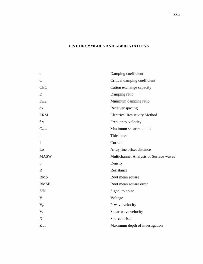
LIST OF SYMBOLS AND ABBREVIATIONS

c

cc

CEC

D

Dmin

dx

ERM

f-v

Gmax

h

I

Lo

MASW

Damping coefficient

Critical damping coefficient

Cation exchange capacity

Damping ratio

Minimum damping ratio

Receiver spacing

Electrical Resistivity Method

Frequency-velocity

Maximum shear modulus

Thickness

Current

Array line offset distance

Multichannel Analysis of Surface waves

ρ

R

Density

Resistance

RMS

RMSE

S/N

V

Vp

Vs

X1

Root mean square

Root mean square error

Signal to noise

Voltage

P-wave velocity

Shear-wave velocity

Source offset

Zmax Maximum depth of investigation

xxiii

LIST OF APPENDIX

APPENDIX TITLE PAGE

A

B

Borehole data for RECESS

Borehole data geotechnical investigation report

173

174

CHAPTER 1

INTRODUCTION

1.1 Research background

Nowadays, geophysical method had been widely used in geotechnical investigation. Some

of the methods which are commonly used are Multichannel Analysis of Surface Waves

(MASW) and Electrical Resistivity Method (ERM). The application of the geophysical

method in soil investigation, especially concerning soft soil is very limited. Hence, this

research focused on the application of geophysical method on the soft soil investigation.

Geophysics method, such as MASW is designed to map spatial variations in the

physical properties of soil. The main advantage of MASW is its ability to take into full

account the complicated nature of seismic waves that always contain noise such as

unwanted higher modes of surface waves, body waves, scattered waves, traffic waves,

etc., as well as fundamental-mode surface waves (Park et al., 2007). The MASW method

is divided into two, which are, active and passive. The active MASW method was

introduced in geophysics in 1999. It adopts the conventional mode of survey using an

active seismic source (e.g., a sledge hammer). It utilizes surface waves propagating

horizontally along the surface of the measurement directly from the impact point to

receivers. MASW also gives shear-wave velocity (Vs) information in either 1-D (depth)

or 2-D (depth and surface location) format at a cost effective and time-efficient manner.

The maximum depth of investigation (zmax) is usually less than 30 m, but this can vary

with the site and type of active source used (Park et al., 2007).

2

The ERM is a geophysical method used to determine the subsurface resistivity

distribution by injecting current into the ground through two current electrodes (C1 and

C2), and measuring the resulting voltage difference at two potential electrodes (P1 and

P2) (Loke, 1999). The Electrical Resistivity Method comprises of a 1-D sounding survey,

2-D imaging survey and 3-D surveys. The ability of 2-D Earth resistivity measurement to

map the electrical resistivity distribution in the Earth allows the estimation of the

subsurface heterogeneity (Slob, 2004).

Soft soil is considered as challenging soil especially due to its special features and

high degree of compressibility. Peat is a representative material of soft soils and classified

as highly organic with organic content more than 75% (Kolay et al., 2011). It is brownish

in color and is formed by decomposed organic matter that have accumulated over a

thousand years, with lack of oxygen and under waterlogged conditions. Peat is well

known to deform and fail under light surcharge load, and it is characterized with low shear

strength (5-20 kPa), high compressibility, high organic content (>75%) and high water

content (>200%) (Zainorabidin and Wijeyesekera, 2007). While, clay is a fine-grained

soil material that become plastic due to their water content and non-plastic when dried.

The clay soil material also combines one or more clay minerals with traces of metal oxides

and organic matter.

1.2 Problem statement

Geotechnical investigation is a critical pre-construction work especially concerning the

soft soil. Various parameters are determined and observed during the investigation which

include surface exploration and subsurface exploration. Dynamic soil properties and soil

stratigraphy are some important parameters in subsurface exploration. Dynamic soil

properties determination especially the shear-wave velocity is considered an important

parameter when dealing with super structure and large construction. As mentioned by

Ivanov et al. (2015), stiffness properties of near surface materials are important for

engineering applications and shear-wave velocity is directly related to stiffness. It is also

a critical parameters in geotechnical earthquake engineering problems. While, the soil

stratigraphy provides description of the soil physical characteristics.

3

The dynamic soil properties and soil stratigraphy are conventionally collected by

boring. This method is intrusive, takes longer time and higher cost before the data are

obtained. The advancement of geophysical method in the past few decades allowed the

investigation of subsurface exploration to be done in more time efficient manner and non-

intrusive way. MASW method and ERM are some example of geophysical method used

in subsurface exploration. The MASW method provides the shear-wave velocity profile

of soil. The shear-wave velocity is one of the important parameters in determining the

shear modulus which is one of the key factors to determine the soil stiffness. While, the

ERM generates the soil stratigraphy and provides the resistivity value of the soil. In this

research, the efficiencies of both methods were investigated to provide better alternatives

in geotechnical investigation in future works.

Several doubts also arises regarding the optimization of the MASW method and

ERM to provide reliable and high accuracy data. Hence, investigation of the data

acquisition configuration and data analyzing are included in this research. The main

purpose is to compare different configuration and data analyzing to achieve the best

results. Therefore, the application of MASW method and ERM with the optimum

configuration, will allow the subsurface exploration of the geotechnical investigation

being done in a more time efficient manner and non-intrusive. Thus, providing knowledge

to develop safer and more economic engineering design with efficient construction

technique.

1.3 Aim

The purpose of this research is to establish soft soil profile using MASW method and

ERM.

1.4 Objectives

This research embarks the following objectives:

i. To determine shear-wave velocity (Vs) profile of soft soil using Multichannel

Analysis of Surface Waves.

4

ii. To identify the effect of different receiver spacing on MASW dispersion curve

resolution.

iii. To determine the soft soil stratigraphy and resistivity value using Electrical

Resistivity Method with complementary from peat sampler and borehole data.

iv. To establish correlation between 1-D shear-wave velocity profile and 1-D

resistivity value.

1.5 Scope of research

This research focused on the establishment of soil profile at Parit Nipah and RECESS.

The active 1-D MASW method and 2-D ERM were used to obtain the shear wave velocity

and resistivity value (soil stratigraphy) respectively. Schlumberger and Wenner protocol

were used for the ERM. The depth of peat layer at Parit Nipah was determined using peat

sampler. While, the depth of soft clay at RECESS was determined from the borehole data

obtained from the previous study.

1.6 Significance of research

The research focused to establish soft soil profile by applying the MASW and ERM. The

data obtained from the analysis can be utilized for many useful applications. First of all,

the shear-wave velocity and shear modulus are critical engineering parameters which

concerned the stiffness of a soil layer. Therefore, good understanding regarding these

dynamic properties allowed the engineers to tackle problems encountered during

construction on soft soil. Next, the resistivity value allowed the determination of water

table and mapping of soil stratigraphy. The data will give further understanding regarding

soft soil, which will give benefit on how to deal with soft soil. These findings also will

help engineer to design sustainable construction on soft soil site. Other than that, the

results obtained may be used as preliminary studies for other soft soil experiments in the

future.

5

1.7 Thesis layout

This thesis comprises the following contents:

i. Chapter 1: This chapter explains the core of this research such as the purpose,

objectives and scope.

ii. Chapter 2: This chapter describes the soft soil characteristics and dynamic

behavior. Geophysical method namely MASW method and ERM also

described with all the necessary terms involved in this research. Previous

researches regarding the topic also included.

iii. Chapter 3: This chapter explains the method used in this research in details.

The method includes 1-D MASW method, 2-D and 1-D ERM and peat

sampler.

iv. Chapter 4: This chapter shows the results obtained from this research. The

results were also discussed and compared with the previous researcher.

v. Chapter 5: This chapter provides the conclusions and recommendation for

further study.

CHAPTER 2

LITERATURE REVIEW

2.1 Introduction

This chapter explained theoretically all the definitions, terms and keywords, related to this

research. It includes the definition of geophysics, seismic, Multichannel Analysis of

Surface Waves (MASW), the applications of seismic, Electrical Resistivity Method

(ERM), resistivity, the applications of resistivity and soft soil. The previous results with

similar interest from previous researchers were also listed.

2.2 Soft soil

The soft soil is considered as the most challenging soils compare to other type of soil.

According to Vermeer and Neher (1999), high degree of compressibility is the special

features of this type of soil. Near-normally consolidated clays, clayey silts and peat are

categorized as soft soil (Vermeer and Neher, 1999).

2.2.1 Peat soil

Peat is an accumulation of partially decayed vegetation or organic matter that is unique to

natural areas called peatlands or mires. In Malaysia, the natural vegetation of peatlands

are mostly peat swamp forest and others comprise of natural vegetation of sedges, grasses

7

and shrubs (International Wetlands, 2010).The peatland ecosystem is the most efficient

carbon sink as peatland plants capture the CO2 which is naturally released. Peat soil

usually dark brown or black in colour, often with distinctive smell (Whitlow, 2001). Peat

is classified as highly organic with organic content more than 75 percent and represent the

extreme form of soft soil (ASTM, 2002). Peat properties reflect the peat environment,

development process of peat and the types of peat-performing plant (Kolay et al., 2011).

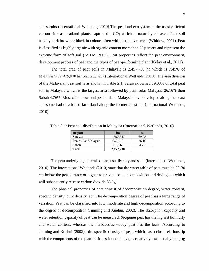
The total area of peat soils in Malaysia is 2,457,730 ha which is 7.45% of

Malaysia’s 32,975,800 ha total land area (International Wetlands, 2010). The area division

of the Malaysian peat soil is as shown in Table 2.1. Sarawak owned 69.08% of total peat

soil in Malaysia which is the largest area followed by peninsular Malaysia 26.16% then

Sabah 4.76%. Most of the lowland peatlands in Malaysia have developed along the coast

and some had developed far inland along the former coastline (International Wetlands,

2010).

Table 2.1: Peat soil distribution in Malaysia (International Wetlands, 2010)

Region ha %

Sarawak 1,697,847 69.08

Peninsular Malaysia 642,918 26.16

Sabah 116,965 4.76

Total 2,457,730

The peat underlying mineral soil are usually clay and sand (International Wetlands,

2010). The International Wetlands (2010) state that the water table of peat must be 20-30

cm below the peat surface or higher to prevent peat decomposition and drying out which

will subsequently release carbon dioxide (CO2).

The physical properties of peat consist of decomposition degree, water content,

specific density, bulk density, etc. The decomposition degree of peat has a large range of

variation. Peat can be classified into low, moderate and high decomposition according to

the degree of decomposition (Jinming and Xuehui, 2002). The absorption capacity and

water retention capacity of peat can be measured. Spagnum peat has the highest humidity

and water content, whereas the herbaceous-woody peat has the least. According to

Jinming and Xuehui (2002), the specific density of peat, which has a close relationship

with the components of the plant residues found in peat, is relatively low, usually ranging

8

from 1.0 to 1.6 Kg m-3. The bulk density of peat, depending upon the ash content,

decomposition degree and components of plant residues, is also low, usually ranging from

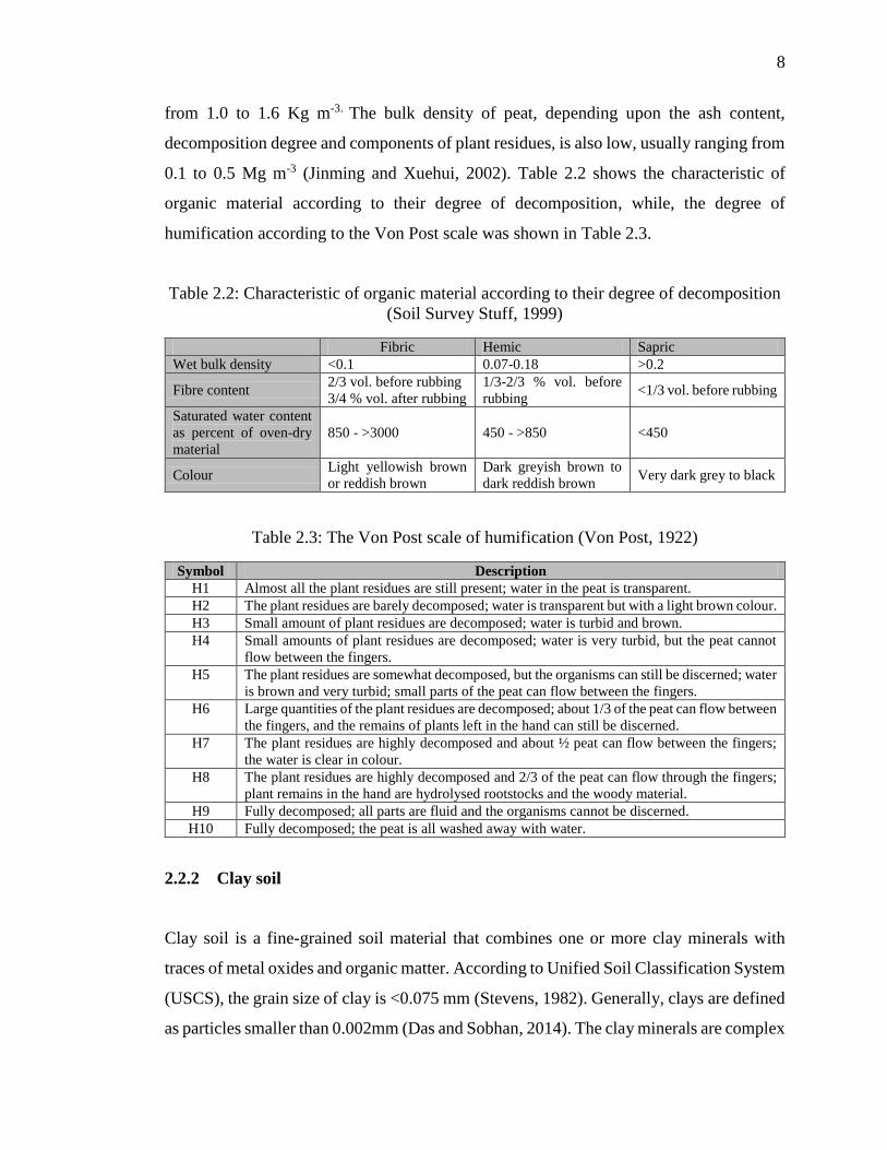
0.1 to 0.5 Mg m-3 (Jinming and Xuehui, 2002). Table 2.2 shows the characteristic of

organic material according to their degree of decomposition, while, the degree of

humification according to the Von Post scale was shown in Table 2.3.

Table 2.2: Characteristic of organic material according to their degree of decomposition

(Soil Survey Stuff, 1999)

Fibric Hemic Sapric

Wet bulk density <0.1 0.07-0.18 >0.2

Fibre content 2/3 vol. before rubbing

3/4 % vol. after rubbing

1/3-2/3 % vol. before

rubbing <1/3 vol. before rubbing

Saturated water content

as percent of oven-dry

material

850 - >3000 450 - >850 <450

Colour Light yellowish brown

or reddish brown

Dark greyish brown to

dark reddish brown Very dark grey to black

Table 2.3: The Von Post scale of humification (Von Post, 1922)

Symbol Description

H1 Almost all the plant residues are still present; water in the peat is transparent.

H2 The plant residues are barely decomposed; water is transparent but with a light brown colour.

H3 Small amount of plant residues are decomposed; water is turbid and brown.

H4 Small amounts of plant residues are decomposed; water is very turbid, but the peat cannot

flow between the fingers.

H5 The plant residues are somewhat decomposed, but the organisms can still be discerned; water

is brown and very turbid; small parts of the peat can flow between the fingers.

H6 Large quantities of the plant residues are decomposed; about 1/3 of the peat can flow between

the fingers, and the remains of plants left in the hand can still be discerned.

H7 The plant residues are highly decomposed and about ½ peat can flow between the fingers;

the water is clear in colour.

H8 The plant residues are highly decomposed and 2/3 of the peat can flow through the fingers;

plant remains in the hand are hydrolysed rootstocks and the woody material.

H9 Fully decomposed; all parts are fluid and the organisms cannot be discerned.

H10 Fully decomposed; the peat is all washed away with water.

2.2.2 Clay soil

Clay soil is a fine-grained soil material that combines one or more clay minerals with

traces of metal oxides and organic matter. According to Unified Soil Classification System

(USCS), the grain size of clay is <0.075 mm (Stevens, 1982). Generally, clays are defined

as particles smaller than 0.002mm (Das and Sobhan, 2014). The clay minerals are complex

9

aluminum silicates composed of two basic units: (1) silica tetrahedron and (2) alumina

octahedron (Das and Sobhan, 2014). Clays become plastic due to their water content and

non-plastic when dried.

The clay particles carry a net negative charge on their surface and in dry condition

the negative charge is balanced by exchangeable cations (Das and Sobhan, 2014).

Therefore, the presence of clay minerals provide cation exchange sites and has a great

influence on the soil conductivity (Huat et al., 2014). According to Long et al. (2012),

high clay content contribute to very low resistivity values.

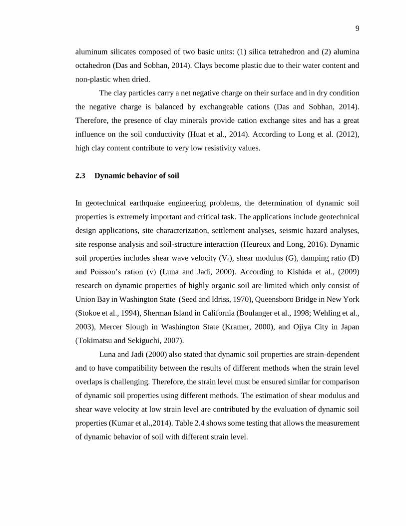
2.3 Dynamic behavior of soil

In geotechnical earthquake engineering problems, the determination of dynamic soil

properties is extremely important and critical task. The applications include geotechnical

design applications, site characterization, settlement analyses, seismic hazard analyses,

site response analysis and soil-structure interaction (Heureux and Long, 2016). Dynamic

soil properties includes shear wave velocity (Vs), shear modulus (G), damping ratio (D)

and Poisson’s ration (v) (Luna and Jadi, 2000). According to Kishida et al., (2009)

research on dynamic properties of highly organic soil are limited which only consist of

Union Bay in Washington State (Seed and Idriss, 1970), Queensboro Bridge in New York

(Stokoe et al., 1994), Sherman Island in California (Boulanger et al., 1998; Wehling et al.,

2003), Mercer Slough in Washington State (Kramer, 2000), and Ojiya City in Japan

(Tokimatsu and Sekiguchi, 2007).

Luna and Jadi (2000) also stated that dynamic soil properties are strain-dependent

and to have compatibility between the results of different methods when the strain level

overlaps is challenging. Therefore, the strain level must be ensured similar for comparison

of dynamic soil properties using different methods. The estimation of shear modulus and

shear wave velocity at low strain level are contributed by the evaluation of dynamic soil

properties (Kumar et al.,2014). Table 2.4 shows some testing that allows the measurement

of dynamic behavior of soil with different strain level.

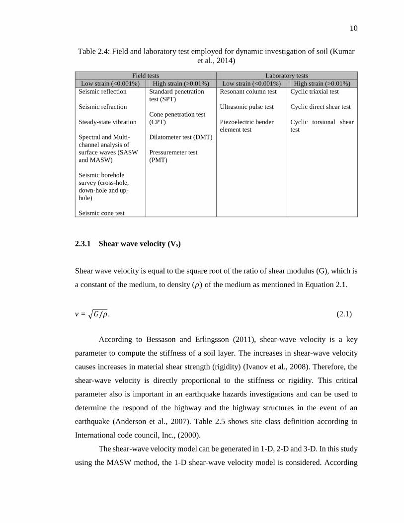
10

Table 2.4: Field and laboratory test employed for dynamic investigation of soil (Kumar

et al., 2014)

Field tests Laboratory tests

Low strain (<0.001%) High strain (>0.01%) Low strain (<0.001%) High strain (>0.01%)

Seismic reflection

Seismic refraction

Steady-state vibration

Spectral and Multi-

channel analysis of

surface waves (SASW

and MASW)

Seismic borehole

survey (cross-hole,

down-hole and up-

hole)

Seismic cone test

Standard penetration

test (SPT)

Cone penetration test

(CPT)

Dilatometer test (DMT)

Pressuremeter test

(PMT)

Resonant column test

Ultrasonic pulse test

Piezoelectric bender

element test

Cyclic triaxial test

Cyclic direct shear test

Cyclic torsional shear

test

2.3.1 Shear wave velocity (Vs)

Shear wave velocity is equal to the square root of the ratio of shear modulus (G), which is

a constant of the medium, to density (𝜌) of the medium as mentioned in Equation 2.1.

v = √𝐺/𝜌. (2.1)

According to Bessason and Erlingsson (2011), shear-wave velocity is a key

parameter to compute the stiffness of a soil layer. The increases in shear-wave velocity

causes increases in material shear strength (rigidity) (Ivanov et al., 2008). Therefore, the

shear-wave velocity is directly proportional to the stiffness or rigidity. This critical

parameter also is important in an earthquake hazards investigations and can be used to

determine the respond of the highway and the highway structures in the event of an

earthquake (Anderson et al., 2007). Table 2.5 shows site class definition according to

International code council, Inc., (2000).

The shear-wave velocity model can be generated in 1-D, 2-D and 3-D. In this study

using the MASW method, the 1-D shear-wave velocity model is considered. According

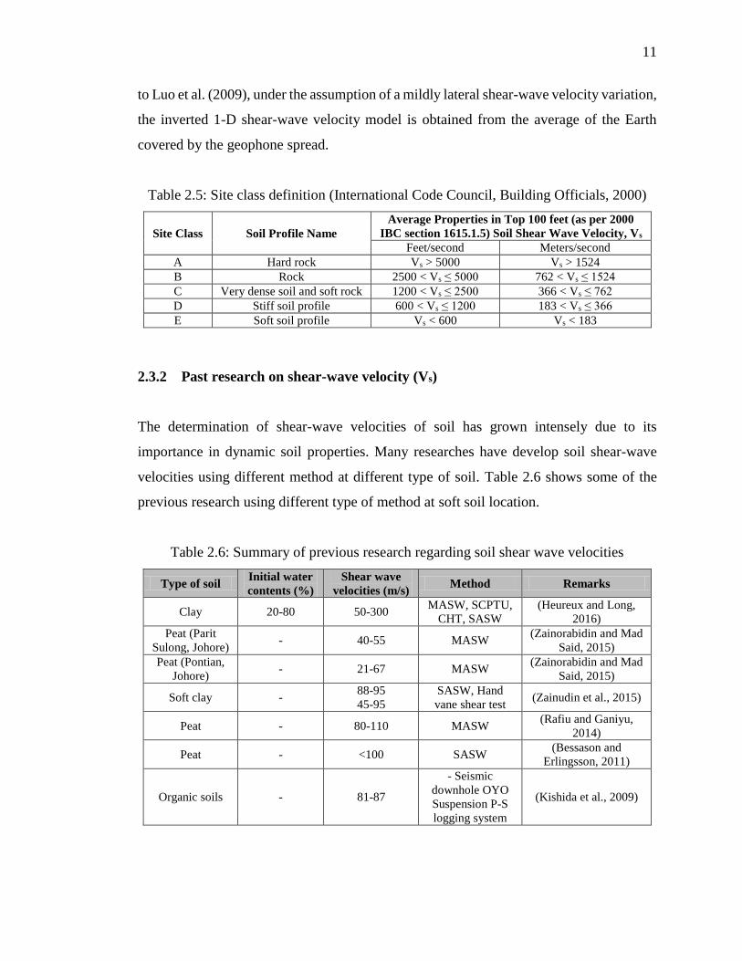
11

to Luo et al. (2009), under the assumption of a mildly lateral shear-wave velocity variation,

the inverted 1-D shear-wave velocity model is obtained from the average of the Earth

covered by the geophone spread.

Table 2.5: Site class definition (International Code Council, Building Officials, 2000)

Site Class Soil Profile Name

Average Properties in Top 100 feet (as per 2000

IBC section 1615.1.5) Soil Shear Wave Velocity, Vs

Feet/second Meters/second

A Hard rock Vs > 5000 Vs > 1524

B Rock 2500 < Vs ≤ 5000 762 < Vs ≤ 1524

C Very dense soil and soft rock 1200 < Vs ≤ 2500 366 < Vs ≤ 762

D Stiff soil profile 600 < Vs ≤ 1200 183 < Vs ≤ 366

E Soft soil profile Vs < 600 Vs < 183

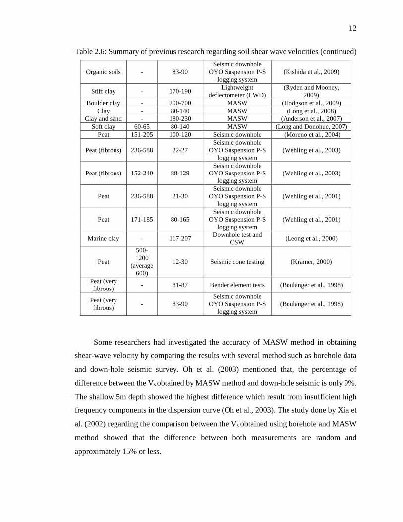
2.3.2 Past research on shear-wave velocity (Vs)

The determination of shear-wave velocities of soil has grown intensely due to its

importance in dynamic soil properties. Many researches have develop soil shear-wave

velocities using different method at different type of soil. Table 2.6 shows some of the

previous research using different type of method at soft soil location.

Table 2.6: Summary of previous research regarding soil shear wave velocities

Type of soil Initial water

contents (%)

Shear wave

velocities (m/s) Method Remarks

Clay 20-80 50-300 MASW, SCPTU,

CHT, SASW

(Heureux and Long,

2016)

Peat (Parit

Sulong, Johore) - 40-55 MASW

(Zainorabidin and Mad

Said, 2015)

Peat (Pontian,

Johore) - 21-67 MASW

(Zainorabidin and Mad

Said, 2015)

Soft clay - 88-95

45-95

SASW, Hand

vane shear test (Zainudin et al., 2015)

Peat - 80-110 MASW (Rafiu and Ganiyu,

2014)

Peat - <100 SASW (Bessason and

Erlingsson, 2011)

Organic soils - 81-87

- Seismic

downhole OYO

Suspension P-S

logging system

(Kishida et al., 2009)

12

Table 2.6: Summary of previous research regarding soil shear wave velocities (continued)

Organic soils - 83-90

Seismic downhole

OYO Suspension P-S

logging system

(Kishida et al., 2009)

Stiff clay - 170-190 Lightweight

deflectometer (LWD)

(Ryden and Mooney,

2009)

Boulder clay - 200-700 MASW (Hodgson et al., 2009)

Clay - 80-140 MASW (Long et al., 2008)

Clay and sand - 180-230 MASW (Anderson et al., 2007)

Soft clay 60-65 80-140 MASW (Long and Donohue, 2007)

Peat 151-205 100-120 Seismic downhole (Moreno et al., 2004)

Peat (fibrous) 236-588 22-27

Seismic downhole

OYO Suspension P-S

logging system

(Wehling et al., 2003)

Peat (fibrous) 152-240 88-129

Seismic downhole

OYO Suspension P-S

logging system


Peat 236-588 21-30

Seismic downhole

OYO Suspension P-S

logging system


Peat 171-185 80-165

Seismic downhole

OYO Suspension P-S

logging system


Marine clay - 117-207 Downhole test and

CSW (Leong et al., 2000)

Peat

500-

1200

(average

600)

12-30 Seismic cone testing (Kramer, 2000)

Peat (very

fibrous) - 81-87 Bender element tests (Boulanger et al., 1998)

Peat (very

fibrous) - 83-90

Seismic downhole

OYO Suspension P-S

logging system

(Boulanger et al., 1998)

Some researchers had investigated the accuracy of MASW method in obtaining

shear-wave velocity by comparing the results with several method such as borehole data

and down-hole seismic survey. Oh et al. (2003) mentioned that, the percentage of

difference between the Vs obtained by MASW method and down-hole seismic is only 9%.

The shallow 5m depth showed the highest difference which result from insufficient high

frequency components in the dispersion curve (Oh et al., 2003). The study done by Xia et

al. (2002) regarding the comparison between the Vs obtained using borehole and MASW

method showed that the difference between both measurements are random and

approximately 15% or less.

13

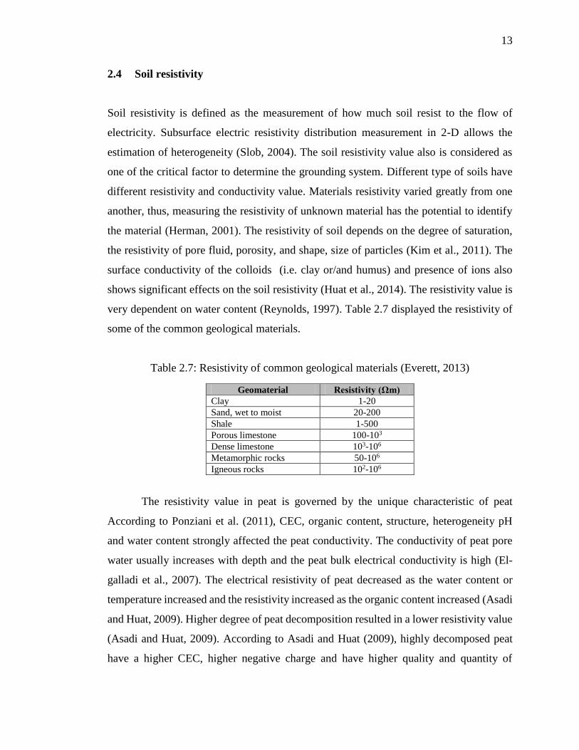
2.4 Soil resistivity

Soil resistivity is defined as the measurement of how much soil resist to the flow of

electricity. Subsurface electric resistivity distribution measurement in 2-D allows the

estimation of heterogeneity (Slob, 2004). The soil resistivity value also is considered as

one of the critical factor to determine the grounding system. Different type of soils have

different resistivity and conductivity value. Materials resistivity varied greatly from one

another, thus, measuring the resistivity of unknown material has the potential to identify

the material (Herman, 2001). The resistivity of soil depends on the degree of saturation,

the resistivity of pore fluid, porosity, and shape, size of particles (Kim et al., 2011). The

surface conductivity of the colloids (i.e. clay or/and humus) and presence of ions also

shows significant effects on the soil resistivity (Huat et al., 2014). The resistivity value is

very dependent on water content (Reynolds, 1997). Table 2.7 displayed the resistivity of

some of the common geological materials.

Table 2.7: Resistivity of common geological materials (Everett, 2013)

Geomaterial Resistivity (Ωm)

Clay 1-20

Sand, wet to moist 20-200

Shale 1-500

Porous limestone 100-103

Dense limestone 103-106

Metamorphic rocks 50-106

Igneous rocks 102-106

The resistivity value in peat is governed by the unique characteristic of peat

According to Ponziani et al. (2011), CEC, organic content, structure, heterogeneity pH

and water content strongly affected the peat conductivity. The conductivity of peat pore

water usually increases with depth and the peat bulk electrical conductivity is high (El-

galladi et al., 2007). The electrical resistivity of peat decreased as the water content or

temperature increased and the resistivity increased as the organic content increased (Asadi

and Huat, 2009). Higher degree of peat decomposition resulted in a lower resistivity value

(Asadi and Huat, 2009). According to Asadi and Huat (2009), highly decomposed peat

have a higher CEC, higher negative charge and have higher quality and quantity of

14

chargeable colloidal particles which resulted in a lower electrical resistivity. The CEC are

the main factor in determination of peat electrical conductivity in normal condition,

whereas at the more acidic site, organic matter and water content are more influential

(Walter et al., 2016).

The presence of clay or the clay layer often shows very low resistivity value. The

presence of clay fraction provide cation exchange sites, thus, contributes to lower

resistivity (Huat et al., 2014). Jakalia et al. (2015) measured the resistivity of saturated

clay and concluded that the presence of saturated clay contributed to very low resistivity

zone. The resistivity of clay is ranged from 1 – 100 ohm.m with 30 – 40 % water content

and 100 – 200 ohm.m for dry clay.

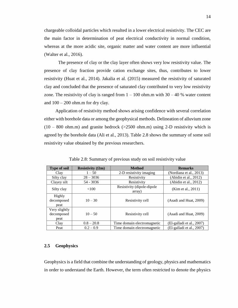
Application of resistivity method shows arising confidence with several correlation

either with borehole data or among the geophysical methods. Delineation of alluvium zone

(10 – 800 ohm.m) and granite bedrock (>2500 ohm.m) using 2-D resistivity which is

agreed by the borehole data (Ali et al., 2013). Table 2.8 shows the summary of some soil

resistivity value obtained by the previous researchers.

Table 2.8: Summary of previous study on soil resistivity value

Type of soil Resistivity (Ωm) Method Remarks

Clay 1 – 50 2-D resistivity imaging (Nordiana et al., 2013)

Silty clay 28 – 3036 Resistivity (Abidin et al., 2012)

Clayey silt 54 - 3036 Resistivity (Abidin et al., 2012)

Silty clay <100 Resistivity (dipole-dipole

array) (Kim et al., 2011)

Highly

decomposed

peat

10 – 30 Resistivity cell (Asadi and Huat, 2009)

Very slightly

decomposed

peat

10 – 50 Resistivity cell (Asadi and Huat, 2009)

Clay 0.8 – 20.8 Time domain electromagnetic (El-galladi et al., 2007)

Peat 0.2 – 0.9 Time domain electromagnetic (El-galladi et al., 2007)

2.5 Geophysics

Geophysics is a field that combine the understanding of geology, physics and mathematics

in order to understand the Earth. However, the term often restricted to denote the physics

15

applied to the ‘solid earth’ which by means, exclude the hydrosphere and atmosphere

(Sharma, 1997). The study of Earth processes includes the laboratory experiments,

computational and theoretical modelling, remote imaging, and direct observation.

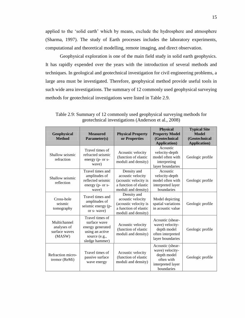
Geophysical exploration is one of the main field study in solid earth geophysics.

It has rapidly expended over the years with the introduction of several methods and

techniques. In geological and geotechnical investigation for civil engineering problems, a

large area must be investigated. Therefore, geophysical method provide useful tools in

such wide area investigations. The summary of 12 commonly used geophysical surveying

methods for geotechnical investigations were listed in Table 2.9.

Table 2.9: Summary of 12 commonly used geophysical surveying methods for

geotechnical investigations (Anderson et al., 2008)

Geophysical

Method

Measured

Parameter(s)

Physical Property

or Properties

Physical

Property Model

(Geotechnical

Application)

Typical Site

Model

(Geotechnical

Application)

Shallow seismic

refraction

Travel times of

refracted seismic

energy (p- or s-

wave)

Acoustic velocity

(function of elastic

moduli and density)

Acoustic

velocity-depth

model often with

interpreting

layer boundaries

Geologic profile

Shallow seismic

reflection

Travel times and

amplitudes of

reflected seismic

energy (p- or s-

wave)

Density and

acoustic velocity

(acoustic velocity is

a function of elastic

moduli and density)

Acoustic

velocity-depth

model often with

interpreted layer

boundaries

Geologic profile

Cross-hole

seismic

tomography

Travel times and

amplitudes of

seismic energy (p-

or s- wave)

Density and

acoustic velocity

(acoustic velocity is

a function of elastic

moduli and density)

Model depicting

spatial variations

in acoustic value

Geologic profile

Multichannel

analyses of

surface waves

(MASW)

Travel times of

surface wave

energy generated

using an active

source (e.g.,

sledge hammer)

Acoustic velocity


moduli and density)

Acoustic (shear-

wave) velocity-

depth model

often interpreted

layer boundaries

Geologic profile

Refraction micro-

tremor (ReMi)

Travel times of

passive surface

wave energy

Acoustic velocity


moduli and density)

Acoustic (shear-

wave) velocity-

depth model

often with

interpreted layer

boundaries

Geologic profile

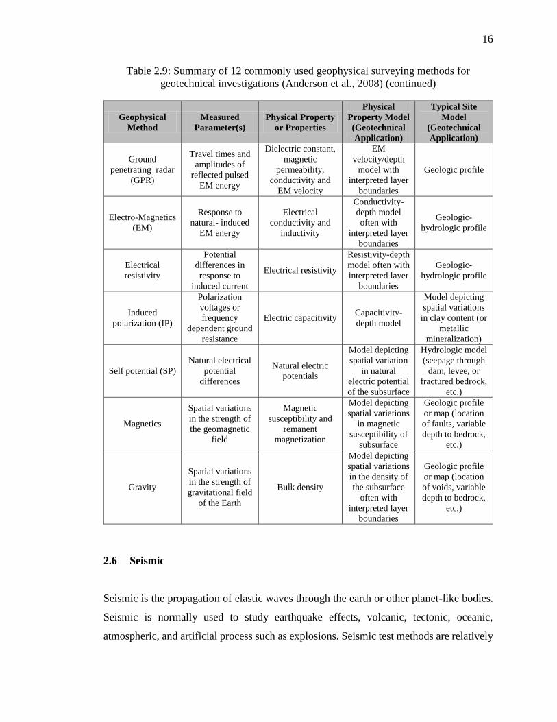
16

Table 2.9: Summary of 12 commonly used geophysical surveying methods for

geotechnical investigations (Anderson et al., 2008) (continued)

Geophysical

Method

Measured

Parameter(s)

Physical Property

or Properties

Physical

Property Model

(Geotechnical

Application)

Typical Site

Model

(Geotechnical

Application)

Ground

penetrating radar

(GPR)

Travel times and

amplitudes of

reflected pulsed

EM energy

Dielectric constant,

magnetic

permeability,

conductivity and

EM velocity

EM

velocity/depth

model with

interpreted layer

boundaries

Geologic profile

Electro-Magnetics

(EM)

Response to

natural- induced

EM energy

Electrical

conductivity and

inductivity

Conductivity-

depth model

often with

interpreted layer

boundaries

Geologic-

hydrologic profile

Electrical

resistivity

Potential

differences in

response to

induced current

Electrical resistivity

Resistivity-depth

model often with

interpreted layer

boundaries

Geologic-

hydrologic profile

Induced

polarization (IP)

Polarization

voltages or

frequency

dependent ground

resistance

Electric capacitivity Capacitivity-

depth model

Model depicting

spatial variations

in clay content (or

metallic

mineralization)

Self potential (SP)

Natural electrical

potential

differences

Natural electric

potentials

Model depicting

spatial variation

in natural

electric potential

of the subsurface

Hydrologic model

(seepage through

dam, levee, or

fractured bedrock,

etc.)

Magnetics

Spatial variations

in the strength of

the geomagnetic

field

Magnetic

susceptibility and

remanent

magnetization

Model depicting

spatial variations

in magnetic

susceptibility of

subsurface

Geologic profile

or map (location

of faults, variable

depth to bedrock,

etc.)

Gravity

Spatial variations

in the strength of

gravitational field

of the Earth

Bulk density

Model depicting

spatial variations

in the density of

the subsurface

often with

interpreted layer

boundaries

Geologic profile

or map (location

of voids, variable

depth to bedrock,

etc.)

2.6 Seismic

Seismic is the propagation of elastic waves through the earth or other planet-like bodies.

Seismic is normally used to study earthquake effects, volcanic, tectonic, oceanic,

atmospheric, and artificial process such as explosions. Seismic test methods are relatively

17

new for stabilizing soil, and most of the tests carried out have been exploratory nature.

The tests employ seismic wave, P-wave, S-wave, Love wave and Rayleigh waves.

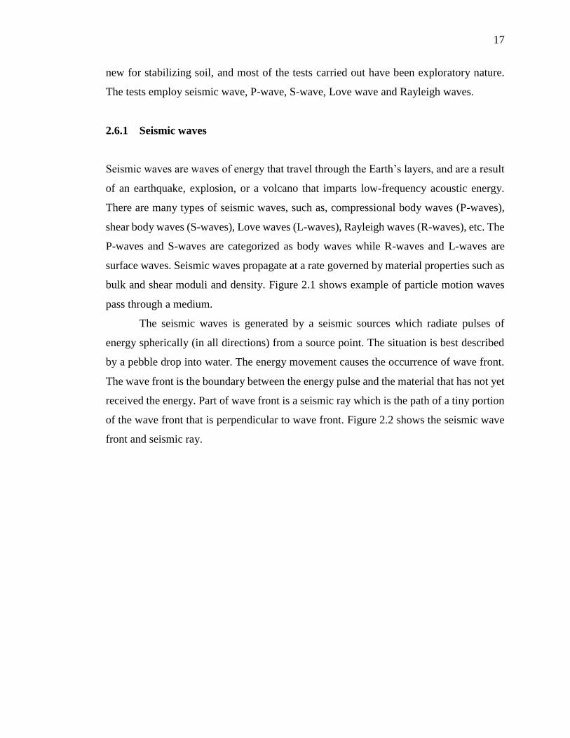
2.6.1 Seismic waves

Seismic waves are waves of energy that travel through the Earth’s layers, and are a result

of an earthquake, explosion, or a volcano that imparts low-frequency acoustic energy.

There are many types of seismic waves, such as, compressional body waves (P-waves),

shear body waves (S-waves), Love waves (L-waves), Rayleigh waves (R-waves), etc. The

P-waves and S-waves are categorized as body waves while R-waves and L-waves are

surface waves. Seismic waves propagate at a rate governed by material properties such as

bulk and shear moduli and density. Figure 2.1 shows example of particle motion waves

pass through a medium.

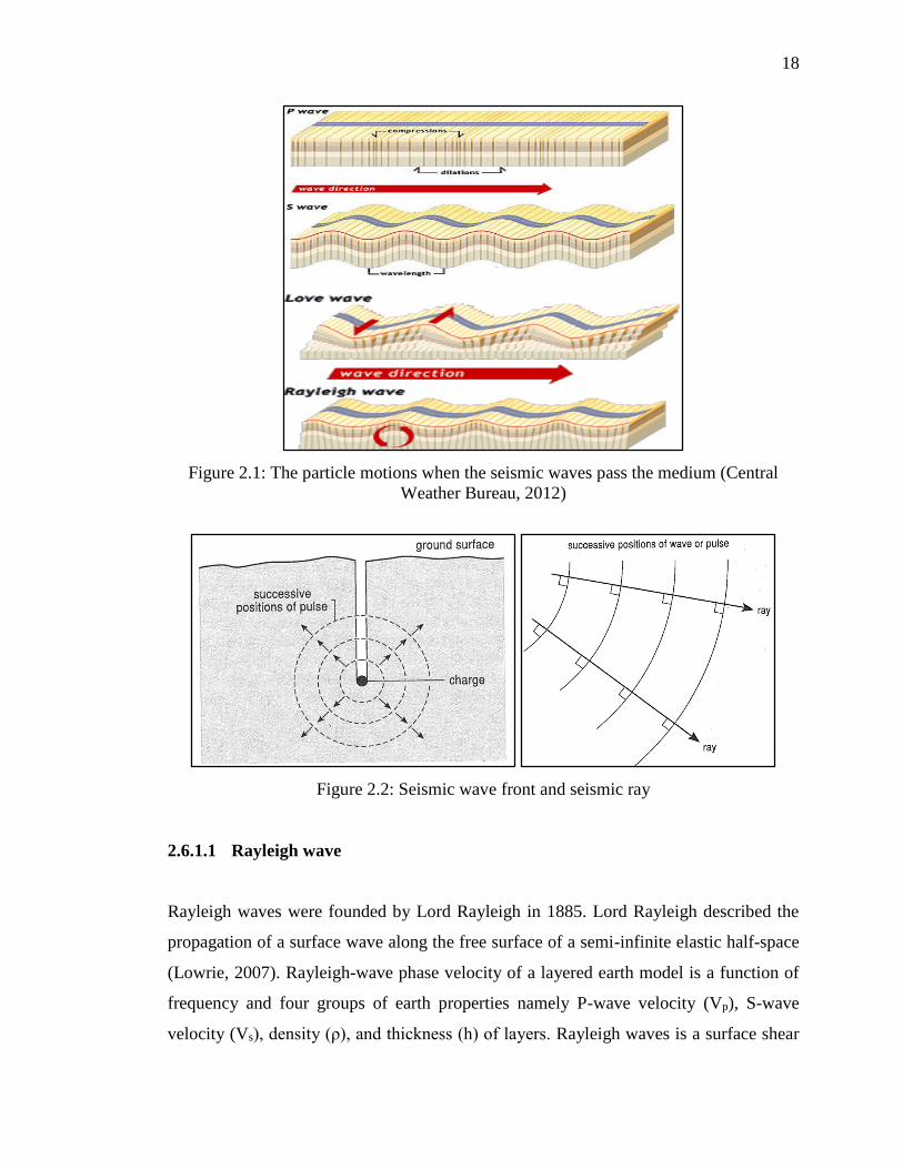
The seismic waves is generated by a seismic sources which radiate pulses of

energy spherically (in all directions) from a source point. The situation is best described

by a pebble drop into water. The energy movement causes the occurrence of wave front.

The wave front is the boundary between the energy pulse and the material that has not yet

received the energy. Part of wave front is a seismic ray which is the path of a tiny portion

of the wave front that is perpendicular to wave front. Figure 2.2 shows the seismic wave

front and seismic ray.

18

Figure 2.1: The particle motions when the seismic waves pass the medium (Central

Weather Bureau, 2012)

Figure 2.2: Seismic wave front and seismic ray

2.6.1.1 Rayleigh wave

Rayleigh waves were founded by Lord Rayleigh in 1885. Lord Rayleigh described the

propagation of a surface wave along the free surface of a semi-infinite elastic half-space

(Lowrie, 2007). Rayleigh-wave phase velocity of a layered earth model is a function of

frequency and four groups of earth properties namely P-wave velocity (Vp), S-wave

velocity (Vs), density (ρ), and thickness (h) of layers. Rayleigh waves is a surface shear

19

waves that makes the ground move up and down in a retrograde elliptical pattern as shown

in Figure 2.1. According to Xia et al. (1999), Rayleigh waves are the result of interfering

P and Sv waves. Particle motion is constrained to the vertical plane consistent with the

direction of wave propagation. In addition, Rayleigh wave has smaller attenuation, high

S/N ratio, stronger immunity of interference and shear wave velocity is the dominant

property (Luo et al., 2009). The longer wavelength surface waves penetrate deeper into

the earth compared to the shorter wavelength (Pei et al., 2006). The strong particle motion

close to the surface of Rayleigh wave is attenuated with depth (Bessason and Erlingsson,

2011). The inversion of the dispersive phase velocity of the surface (Rayleigh and/or

Love) wave will produce the S-wave velocity (Xia et al., 1999).

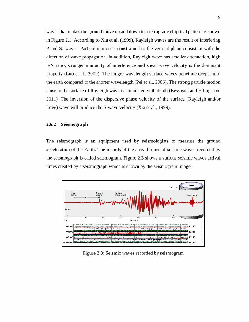
2.6.2 Seismograph

The seismograph is an equipment used by seismologists to measure the ground

acceleration of the Earth. The records of the arrival times of seismic waves recorded by

the seismograph is called seismogram. Figure 2.3 shows a various seismic waves arrival

times created by a seismograph which is shown by the seismogram image.

Figure 2.3: Seismic waves recorded by seismogram

20

2.7 Multichannel analysis of surface waves (MASW)

MASW is a seismic exploration method evaluating ground stiffness in 1-D, 2-D, and 3-D

formats for various types of Geotechnical engineering projects. Since its first introduction

in the late 1990s by the Kansas Geological Survey (Park et al., 1999), it has been utilized

by many practitioners and researched by many investigators worldwide. The MASW

exploits multichannel recording and processing techniques in order to solve the problem

associated with the Spectral Analysis of Surface Waves (SASW) (Huang and Mayne,

2008). According to Xia et al., (2002), MASW is an environmentally-friendly method for

estimation of shear-wave velocity with depth. It is also economically reliable compared

to several other method. This survey deals with surface waves in the lower frequencies

range 1-30 Hz and much shallower depth of investigation (Park et al., 2007). In the matter

of time for example, MASW method needed approximately a few minutes to obtain the

data.

2.7.1 Active MASW method

The active MASW method generates surface waves actively through an impact source

like a sledge hammer. This method is time efficient as the result can be obtained directly.

Figure 2.4 shows an illustration of different type of waves in MASW method. The

investigation depth is usually less than 30 m (Park et al., 2007). The data acquisition for

active MASW survey is related to several parameters. The list of the optimum parameters

for the data acquisition is as shown in Table 2.10. Although slight variation in any

parameter could happen at different site or condition.

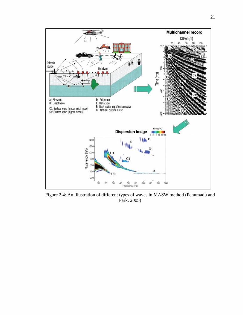
21

Figure 2.4: An illustration of different types of waves in MASW method (Penumadu and

Park, 2005)

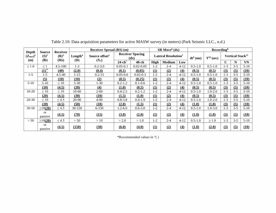
Table 2.10: Data acquisition parameters for active MASW survey (in meters) (Park Seismic LLC., n.d.)

Depth

(Zmax)1

(m)

Source

(S)2

(lb)

Receiver

(R)3

(Hz)

Receiver Spread (RS) (m) SR Move6 (dx) Recording8

Length4

(D)

Source offset5

(X1)

Receiver Spacing

(dx) Lateral Resolution7

dt9 (ms) T10 (sec) Vertical Stack11

24-ch* 48-ch High Medium Low C N VN

≤ 1.0 ≤ 1 4.5-100 1-3 0.2-3.0 0.05-0.1 0.02-0.05 1-2 2-4 4-12 0.5-1.0 0.5-1.0 1-3 3-5 5-10

(1)** (40) (2.0) (0.4) (0.1) (0.05) (1) (2) (4) (0.5) (0.5) (3) (5) (10)

1-5 1-5 4.5-40 1-15 0.2-15 0.05-0.6 0.02-0.3 1-2 2-4 4-12 0.5-1.0 0.5-1.0 1-3 3-5 5-10

(5) (10) (10) (2) (0.5) (0.25) (1) (2) (4) (0.5) (0.5) (3) (5) (10)

5-10 5-10 ≤ 10 5-30 1-30 0.2-1.2 0.1-0.6 1-2 2-4 4-12 0.5-1.0 0.5-1.0 1-3 3-5 5-10

(10) (4.5) (20) (4) (1.0) (0.5) (1) (2) (4) (0.5) (0.5) (3) (5) (10)

10-20 ≥ 10 ≤ 10 10-60 2-60 0.4-2.5 0.2-1.2 1-2 2-4 4-12 0.5-1.0 1.0-2.0 1-3 3-5 5-10

(20) (4.5) (30) (10) (1.5) (1.0) (1) (2) (4) (0.5) (0.5) (3) (5) (10)

20-30 ≥ 10 ≤ 4.5 20-90 4-90 0.8-3.8 0.4-1.9 1-2 2-4 4-12 0.5-1.0 1.0-2.0 1-3 3-5 5-10

(20) (4.5) (50) (10) (2.0) (1.5) (1) (2) (4) (1.0) (1.0) (3) (5) (10)

30-50 ≥10(20) ≤ 4.5 30-150 6-150 1.2-6.0 0.6-3.0 1-2 2-4 4-12 0.5-1.0 1.0-3.0 1-3 3-5 5-10

or

passive (4.5) (70) (15) (3.0) (2.0) (1) (2) (4) (1.0) (1.0) (3) (5) (10)

> 50 ≥10(20) ≤ 4.5 > 50 > 10 > 2.0 > 1.0 1-2 2-4 4-12 0.5-1.0 ≥ 1.0 1-3 3-5 5-10

or

passive (4.5) (150) (30) (6.0) (4.0) (1) (2) (4) (1.0) (2.0) (3) (5) (10)

*Recommended values in “( )

23

2.8 Factors influencing MASW data acquisition

In every research, there are always factors that affect the testing or result obtained. Careful

action need to be taken to minimize the error caused by these factors. In this subtopic,

several factors that related to MASW data acquisition are stated and discussed. Those

factors are seismograph setting, equipment configuration, topography, and dispersion

curve plotting.

2.8.1 Seismograph configuration

The seismograph is an equipment used to record the waves received by the sensor. In this

study, ABEM Terraloc MK8 is used to record the waves. The critical configuration for

the seismograph involved the acquisition setup, receiver spread and layout geometry.

2.8.1.1 Acquisition setup

The acquisition setup interface involves the configuration for the setup, trig, noise and

filters. For the setup, it involves the sampling interval, number of samples, pre-trig or

delay, number of stacks, stack mode and re-arm mode. The pre-trig or delay, stack mode

and re-arm mode, can be configured according to the needs during the data acquisition.

The sampling interval and number of sample are critical as it will determine the recording

time for each data set. Short recording time will cause incomplete data set recorded. While,

long recording time increase the possibility of recording ambient noise (Taipodia and Dey,

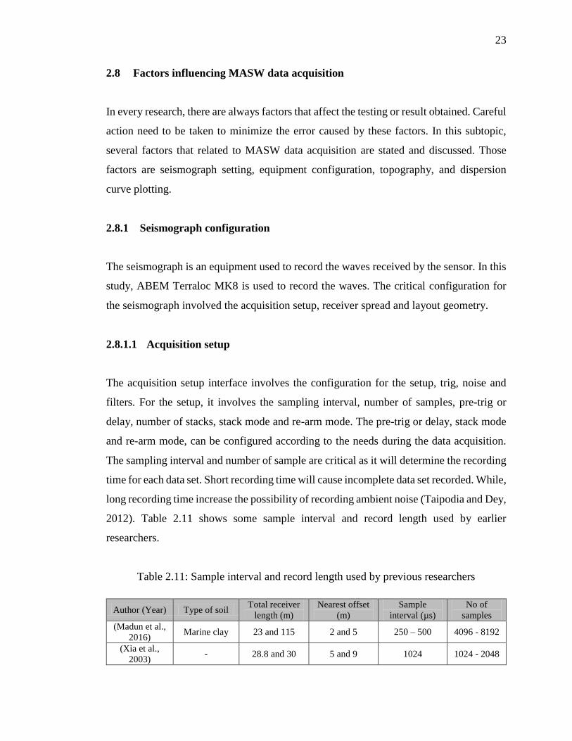
2012). Table 2.11 shows some sample interval and record length used by earlier

researchers.

Table 2.11: Sample interval and record length used by previous researchers

Author (Year) Type of soil Total receiver

length (m)

Nearest offset

(m)

Sample

interval (µs)

No of

samples

(Madun et al.,

2016) Marine clay 23 and 115 2 and 5 250 – 500 4096 - 8192

(Xia et al.,

2003) - 28.8 and 30 5 and 9 1024 1024 - 2048

24

The number of stacks is determined according to the environment and type of soil

involves. When the environment involves high noise due to traffic such as at urban

location, high number of stacking is needed to increase the signal-to-noise ratio. Limited

noise such as at rural area need less number of stacking as the signal-to-noise ratio is

already high. However, the type of soil also affect the determination of number of

stacking. Weak soil such as highly organic soil will interrupt the wave travel during data

acquisition which directly affect the S/N ratio. Therefore, by increasing the number of

stacking will improved the S/N ratio. As for the hard soil, the wave travel will be less

affected which provide high signal-to-noise ratio.

The trigger setup involved the configuration of trig input mode, trig input level,

external trig/arm out mode and verify timeout (ms). High value of input level increased

the sensitivity of the trigger which means lower signal level is needed to trig the terraloc

(“Seismic System Reference Manual for ABEM Terraloc ® Mk6 v2 and Mk8 with ABEM

SeisTW for Windows XP ® 2009-05-19,” 2009). The environment noise should also be

consider to prevent auto-trigger due to high sensitivity trigger. The noise monitor can be

set on or off. However, it is recommended to turn it on to allow noise monitoring before

and during data acquisition. The damping value define the sensitivity of the recorder.

Lower damping value will increase the sensitivity of source detection. But, with the

presence of high noise, it is recommended to set higher value to prevent auto-triggered by

the noise. The threshold level does not affect much in this study, therefore, it is set as zero.

The filter setting allows the data filtering during data acquisition. However, it is

best to turn of this setting to produce high quality data with minimum altering. This is to

provide engineer with the real in-situ data.

2.8.1.2 Receiver spread

The receiver spread interface is used to ensure the trace number and the channels are

synchronize accordingly to allow correct wave data set recorded. Wrong synchronization

will cause the recorded waves to be placed at different location. Although this action is

reversible during the data analysis, proper configuration will ease the process and save

time.

REFERENCES

Abdul-Nafiu, A. K., Mohd. Nordin, M. N., Abdullah, K., Saheed, I. K., & Abdullah, A.

(2013). Effects of electrode spacing and inversion techniques on the efficacy of 2D

resistivity imaging to delineate subsurface features. American Journal of Applied

Sciences, 10(1), 64–72.

Abem (2010). ABEM SAS 4000 Instruction Manual, (33), 148.

Abidin, M. H. Z., Saad, R., Ahmad, F., Wijeyesekera, D. C., & Baharuddin, M. F. T.

(2012). Integral Analysis of Geoelectrical (Resistivity) and Geotechnical (SPT) Data

in Slope Stability Assessment, 1(2), 305–316.

Agus, S., Ismail, B., & Amirkhan, S. (2010). The Performance Evaluation of Lightweight

Concrete Piles on UTHM’s Soft Soil under Static and Dynamic Loading Tests.

International Journal of Integrated Engineering, 53–65.

Aizebeokhai, A. P., Oyeyemi, K. D., & Kayode, O. T. (2015). Multiple-gradient array for

near-surface electrical resistivity tomography. Near-Surface Asia Pacific

Conference, 324–327.

Ali, N., Saad, R., & Mohd Muztaza, N. (2013). Integration of Seismic Refraction and 2D

Electrical Resistivity in Locating Geological Contact. Open Journal of Geology,

03(02), 7–12.

Anderson, N., Thitimakorn, T., Hoffman, D., Stephenson, R., & Luna, R. (2007). A

Comparison of Four Geophysical Methods for Determining the Shear Wave Velocity

of Soils. Engineering, XIII(1), 11–23.

Apostolopoulos, G. (2008). Combined Schlumberger and dipole-dipole array for

hydrogeologic applications. Geophysics, 73(5), 189–195.

Asadi, A., & Huat, B. B. K. (2009). Electrical resistivity of tropical peat. Electronic

Journal of Geotechnical Engineering, 14, 1–9.

165

ASTM (2002). ASTM D4427-02 Standard Classification of Peat Samples by Laboratory

Testing. American Society of Testings and Methods, ASTM, 92(Reapproved), 5–7.

Baines, D., Smith, D. G., Froese, D. G., Bauman, P., & Nimeck, G. (2002). Electrical

resistivity ground imaging (ERGI): A new tool for mapping the lithology and

geometry of channel-belts and valley-fills. Sedimentology, 49(3), 441–449.

Bessason, B., & Erlingsson, S. (2011). Shear wave velocity in surface sediments. Jokull,

51–64.

Boulanger, R. W., Arulnathan, R., Harder Jr., L. F., Torres, R. A., & Driller, M. W. (1998).

Dynamic Properties of Sherman Island Peat. Journal of Geotechnical and

Geoenvironmental Engineering, 124(1), 12–20.

Burger, H. R., Sheehan, A. F., & Jones, C. H. (2006). Introduction to Applied Geophysics.

New York: W.W. Norton & Company, Inc.

Das, B. M., & Sobhan, K. (2014). Principles of Geotechnical Engineering (Eighth).

United States of America: Cengage Learning.

Dey, T. and, Taipodia, J., & Dey, A. (2012). A Review of Active and Passive MASW

Techniques. Egceg.

Edwards, L. S. (1977). A Modified Pseudosection for Resistivity and Ip. Geophysics,

42(5), 1020–1036.

Eijkelkamp Agrisearch Equipment (2014). Peat Sampler Operating Instruction.

Netherlands: Eijkelkamp Agrisearch Equipment.

El-galladi, A., El-qady, G., & Metwaly, M. (2007). Mapping Peat Layer Using Surface

Geoelectrical Methods at Mansoura Environs, Nile Delta, Egypt, 34, 59–78.

Everett, M. E. (2013). Near-Surface Applied Geophysics (First edit). Cambridge:

Cambridge University Press.

Geo Services (2001). Geotechnical Investigation Report for "Cadangan Membina dan

Menyiapkan Sebuah Bangunan Pusat Mahasiswa di Kolej Universiti Teknologi Tun

Hussein Onn, Mukim Parit Raja, Daerah Batu Pahat, Johor Darul Takzim. Technical

Report.

Google Maps (n.d.-a). Jalan Kampung Parit Nipah Darat. Retrieved August 27, 2016, from

https://goo.gl/maps/ZX1kZEddfN42

Google Maps (n.d.-b). Recess UTHM. Retrieved August 30, 2016, from

166

https://goo.gl/maps/sHktvoENyNM2

Griffiths, D. H., & Barker, R. D. (1993). Two-dimensional resistivity imaging and

modelling in areas of complex geology. Journal of Applied Geophysics, 29(3-4),

211–226.

Hayashi, H., Yamazoe, N., Mitachi, T., Tanaka, H., & Nishimoto, S. (2012). Coefficient

of earth pressure at rest for normally and overconsolidated peat ground in Hokkaido

area. Soils and Foundations, 52(2), 299–311.

Herman, R. (2001). An introduction to electrical resistivity in geophysics. American

Journal of Physics, 69, 943.

Heureux, J. S. L., & Long, M. (2016). Correlations between shear wave velocity and

geotechnical parameters in Norwegian clays. Proceedings of the 17th Nordic

Geotechnical Meeting, 299–308.

Hodgson, J. A., Donohue, S., O’Connell, Y., Krahn, H., Reid, G., & Young, M. (2009).

A geophysical journey around Ireland. First Break, 27(8), 35–42.

Huat, B. B. K., Prasad, A., Asadi, A., & Kazemian, S. (2014). Geotechnical of Organic

Soils and Peat.

Huat, B., Prasad, A., Asadi, A., & Kazemian, S. (2014). Geotechnics of Organic Soils and

Peat. London: CRC Press.

International Code Council. (2000). International building code. Falls Church,

Va.:International Code Council.

International Wetlands. (2010). A Quick Scan of Peatlands in Malaysia, 86.

Ivanov, J., Miller, R. D., Morton, S., & Peterie, S. (2015). Dispersion-Curve Imaging

Considerations When Using Multichannel Analysis of Surface Wave (MASW)

Method. Symposium on the Application of Geophysics to Engineering and

Environmental Problems 2015, 556–566.

Ivanov, J., Miller, R. D., & Tsoflias, G. (2008). Some Practical Aspects of MASW

Analysis and Processing. Symposium on the Application of Geophysics to

Engineering and Environmental Problems 2008, 1186–1198.

Jabatan Mineral dan Geosains Malaysia (n.d.). Geological Map of Peninsular Malaysia.

Retrieved July 18, 2016, from http://www.jmg.gov.my/add_on/mt/smnjg/tiles/

Jakalia, I. S., Aning, A., Preko, K., Sackey, N., & K., D. S. (2015). Implications of Soil

167

Resistivity Measurements Using The Electrical Resistivity Method : A Case Study

of A Maize Farm Under Different Soil Preparation Modes At KNUST Agricultural

Research Station, Kumasi. International Journal of Scientific & Technology

Resesarch, 4(1), 9–18.

Jinming, H., & Xuehui, M. (2002). Physical and Chemical Properties of Peat.

Encyclopedia of Life Support Systems: Coal, Oil Shale, Natural Bitumen, Heavy Oil

and Peat, II.

Kim, M. Il, Kim, J. S., Kim, N. W., & Jeong, G. C. (2011). Surface geophysical

investigations of landslide at the Wiri area in Southeastern Korea. Environmental

Earth Sciences, 63(5), 999–1009.

Kishida, T., Wehling, T. M., Boulanger, R. W., Driller, M. W., & Stokoe, K. H. (2009).

Dynamic Properties of Highly Organic Soils from Montezuma Slough and Clifton

Court. Journal of Geotechnical and Geoenvironmental Engineering, 135(4), 525–

532.

Kolay, P. K., Sii, H. Y., & Taib, S. N. L. (2011). Tropical Peat Soil Stabilization using

Class F Pond Ash from Coal Fired Power Plant. International Journal of Civil and

Environmental Engineering, 3(2), 79–83.

Kramer, S. L. (2000). Dynamic Response of Mercer Slought Peat. Journal of

Geotechnical and Geoenvironmental Engineering, 90, 504–510.

Kumar, S. S., Murali Krishna, A., & Dey, A. (2014). Parameters Influencing Dynamic

Soil Properties: A Review Treatise. International Journal of Innovative Research in

Science, 3(4), 47–60.

Leong, E. C., Anand, S., Cheong, H. K., & Pan, T. C. (2000). In-situ measurement of

shear wave velocities at two soft soil sites in Singapore, (161).

Ling, F. N. L., Kassim, K. A., Tarmizi, A., Karim, A., Tiong, K., & Tan, C. K. (2013).

Geochemistry Properties of Southern Malaysian Organic Soil, 287, 1340–1344.

Loke, M. H. (2004). Tutorial : 2-D and 3-D electrical imaging surveys. Geotomo Software

Malaysia, 127.

Loke, M. H. (1999). Electrical imaging surveys for environmental and engineering

studies. Cangkat Minden Lorong, 6574525, 63.

Loke, M. H. (2010). Res2DInv ver 3.59.102. Geoelectrical Imaging 2D and 3D.

168

Instruction Manual. Geotomo Software.

Loke, M. H., Wilkinson, P. B., & Chambers, J. E. (2010). Fast computation of optimized

electrode arrays for 2D resistivity surveys. Computers and Geosciences, 36(11),

1414–1426.

Long, M., & Donohue, S. (2007). In situ shear wave velocity from multichannel analysis

of surface waves (MASW) tests at eight Norwegian research sites. Canadian

Geotechnical Journal, 44(5), 533–544.

Long, M., Donohue, S., L’Heureux, J. S., Solberg, I. L., Rønning, J. S., Limacher, R.,

Lecomte, I. (2012). Relationship between electrical resistivity and basic geotechnical

parameters for marine clays. Canadian Geotechnical Journal, 49(10), 1158–1168.

Long, M., Dublin, C., Connor, P. O., Geoservices, A., & Wexford, C. (2008). Rapid, cost-

effective and accurate determination of in-situ stiffness using MASW at Bothkennar.

Ground Engineering, 43–46.

Lowrie, W. (2007). Fundamentals of Geophysics (Second Ed.). Cambridge: Cambridge

University Press.

Luna, R., & Jadi, H. (2000). Determination of dynamic soil properties using geophysical

methods. First International Conference on the Application of Geophysical and NDT

Methodologies to Transportation Facilities and Infrastructure, 1–15.

Luo, Y., Xia, J., Liu, J., Xu, Y., & Liu, Q. (2009). Research on the middle-of-receiver-

spread assumption of the MASW method. Soil Dynamics and Earthquake

Engineering, 29(1), 71–79.

Madun, A., Ahmad Supa’at, M. E., Ahmad Tajudin, S. A., Zainalabidin, M. H., Sani, S.,

& Yusof, M. F. (2016). Soil investigation using Multichannel Analysis of Surface

Wave (MASW) and borehole. ARPN Journal of Engineering and Applied Sciences,

11(6), 3759–3763.

Mansor, H., & Zainorabidin, A. (2016). Stress-Strain Behavior of Parit Nipah Peat Stress-

Strain Behavior of Parit Nipah Peat.

Miele, M., Laymon, D., Gilkeson, R., & Michelotti, R. (1996). Rectangular Schlumberger

Resistivity Arrays for Delineating Vadose Zone Clay‐Lined Fractures in Shallow

Tuff. Symposium on the Application of Geophysics to Engineering and

Environmental Problems 1996, 397–408.

169

Mohamed, A. M. E., El, A. S. A. A., Azim, F. A., & Taha, M. A. (2013). Site-specific

shear wave velocity investigation for geotechnical engineering applications using

seismic refraction and 2D multi-channel analysis of surface waves. NRIAG Journal

of Astronomy and Geophysics, 2(1), 88–101.

Moreira, C. A., Lapola, M. M., & Carrara, A. (2016). Comparative analyzes among

electrical resistivity tomography arrays in the characterization of flow structure in

free aquifer. Geofisica Internacional, 55, 119–129.

Moreno, C. a, Rodriguez, E. E., & Characterization, P. (2004). Dynamic Behavior of

Bogota’s Subsoil Peat and It’s Effect in Seismic Wave Propagation. Stress: The

International Journal on the Biology of Stress, 1–15.

Morris, M., Ronning, J. S., & Lile, O. B. (1997). Detecting lateral resistivity

inhomogeneities with the Schlumberger array. Geophysical Prospecting, 45(3), 435–

448.

Neil, A., Neil, C., Rick, H., & Phil, S. (2008). Geophysical Methods Commonly Employed

for Geotechnical Site Characterization. Transportation.

Nordiana, M. M., Saad, R., Nawawi, M. N. M., Azwin, I. N., & Mohamad, E. T. (2013).

Case Study: Shallow Subsurface Geology Mapping Using 2-D Resistivity Imaging

with EHR Technique. APCBEE Procedia, 5, 134–140.

Oh, Y., Jeong, H., Lee, Y., & Shon, H. (2003). Safety Evaluation of Rock‐Fill Dam by

Seismic (MASW) and Resistivity Methods. Symposium on the Application of

Geophysics to Engineering and Environmental Problems 2003, 1377–1386.

Park Seismic LLC. (n.d.). MASW-Data Acquisition. Retrieved June 16, 2016, from

http://www.masw.com/DataAcquisition.html

Park, C. B., & Carnevale, M. (2010). Optimum MASW Survey — Revisit after a Decade

of Use. GeoFlorida 2010: Advances in Analysis, Modeling & Design, (Gsp 199),

1303–1312.

Park, C. B., Miller, R. D., & Xia, J. (2007). Multichannel analysis of surface waves. The

Leading Edge, 26(1), 60–64.

Park, C. B., Miller, R. D., & Xia, J. (2001). Offset and Resolution of Dispersion Curve in

Multichannel Analysis of Surface Waves (MASW). Symposium on the Application

of Geophysics to Engineering and Environmental Problems 2001, SSM4–SSM4.

170

Park, C. B., Miller, R.D., & Xia, J. (1999). Multichannel analysis of surface waves.

Geophysics, 64, 800–808.

Park, C. B., Miller, R., & Xia, J. (1997). Multi-Channel Analysis of Surface Waves

(MASW) - A summary report of technical aspects, experimental results and

perspective, 26.

Park, C. B., Miller, R. D., & Miura, H. (2002). Optimum field parameters of an MASW

survey. Society of Exploration Geophysicists of Japan, Tokyo.

Pei, D., John N. Louie, & Satish K. Pullammanappallil. (2006). Annual International

Meeting, SEG, Expanded Abstracts, 1172–1175.

Penumadu, D., & Park, C. B. (2005). Multichannel Analysis of Surface Wave (MASW)

Method for Geotechnical Site Characterization. Earthquake Engineering and Soil

Dynamics, 1–10.

Ponziani, M., Slob, E. C., & Vanhala, H. (2011). Influence of Water Content on the

Electrical Conductivity of Peat, I(1), 14–21.

Popescu, M., Șerban, R. D., Dea, P. U. R., & Onaca, A. (2016). Conventional Geophysical

Surveys for Landslide Investigations: Two Case Studies From Romania, 11(1), 281–

292.

Rafiu, B. A., & Ganiyu, O. B. (2014). Estimation of Shear Wave Velocity for Near-

surface Characterisation; Case Study: Ifako / Gbagada Area of Lagos State, S. W.

Nigeria, 4(5), 831–840.

Reynolds, J. M. (1997). An introduction to applied and environmental geophysics. New

York: Wiley.

Reynolds, J. M. (2011). Electrical resistivity sounding and tomography. Technical

Summary Sheet No. 2, (2), 1–2.

Ryden, N., & Mooney, M. A. (2009). Analysis of surface waves from the light weight

deflectometer. Soil Dynamics and Earthquake Engineering, 29(7), 1134–1142.

Seed, H. B., & Idriss, I. M. (1970). Analyses of ground motions at Union Bay, Seattle

during earthquakes and distant nuclear blasts. Bulletin of the Seismological Society

of America, 60(1), 125–136.

Seismic System Reference Manual for ABEM Terraloc ® Mk6 v2 and Mk8 with ABEM

SeisTW for Windows XP ® 2009-05-19. (2009).

171

Slob, E. (2004). Optimal acquisition and synthetic electrode arrays. 74th Ann. Internat.

Mtg. 1389–1392.

Soil Survey Stuff. (1999). Soil Taxonomy - A Basic System of Soil Classification for

Making and Interpeting Soil Surveys. United States Department of Agriculture,

Natural Resources Conservarion Service, (Second Edition), 1–871.

Stevens, J. (1982). Unified Soil Classification System. Civil Engineering-ASCE, 52(12),

61–62.

Stokoe, K. H., Wright, S. G., Bay, J. A., & Roesset, J. M. (1994). Characterization of

geotechnical sites by SASW method. Geophysical Characterization of Sites, 15–25.

Telford, W. M., Geldart, L. P., & Sheriff, R. E. (1990). Applied Geophysics (Second Ed.).

Cambridge: Cambridge University Press.

Tokimatsu, K., & Sekiguchi, T. (2007). Effects of dynamic properties of peat on strong

ground motions during 2004 mid Niigata prefecture earthquake. In Proc., 4th Int.

Conf. on Earthquake Geotechnical Engineering, Thessaloniki, (1531).

Vermeer, P., & Neher, H. (1999). A soft soil model that accounts for creep. Beyond 2000

in Computational Geotechnics, 249–261.

Von Post, L. (1922). Sveriges geologiska undersoknings torvinventering och nagre av dess

hittills vunna resultat. Sr. Mosskulturfor, Tidskr 1, 1–27.

Walter, J., Hamann, G., Lück, E., Klingenfuss, C., & Zeitz, J. (2016). Stratigraphy and

soil properties of fens: Geophysical case studies from northeastern Germany. Catena,

142, 112–125.

Wehling, T. M., Boulanger, R. W., Arulnathan, R., Harder, L. F., & Driller, M. W. (2003).

Nonlinear Dynamic Properties of a Fibrous Organic Soil. Journal of Geotechnical

and Geoenvironmental Engineering, 129(10), 929–939.

Wehling, T. M., Boulanger, R. W., Harder, L. F., & Driller, M. W. (2001). Dynamic

Properties of Sherman Island Peat: Phase II Study, (March 2001).

Whitlow, R. (2001). Basic Soil Mechanics (Fourth Ed.). England: Prentice Hall.

Xia, J. (2014). Estimation of near-surface shear-wave velocities and quality factors using

multichannel analysis of surface-wave methods. Journal of Applied Geophysics,

103, 140–151.

Xia, J., Miller, R. D., & Park, C. B. (1999). Estimation of near-surface shear-wave velocity

172

by inversion of Rayleigh waves. Geophysics, 64(3), 691.

Xia, J., Miller, R. D., Park, C. B., Hunter, J. A., Harris, J. B., & Ivanov, J. (2002).

Comparing shear-wave velocity profiles inverted from multichannel surface wave

with borehole measurements. Soil Dynamics and Earthquake Engineering, 22(3),

181–190.

Xia, J., Miller, R. D., Park, C. B., & Tian, G. (2003). Inversion of high frequency surface

waves with fundamental and higher modes, 52, 45–57.

Xu, Y., Xia, J., & Miller, R. D. (2006). Quantitative estimation of minimum offset for

multichannel surface-wave survey with actively exciting source. Journal of Applied

Geophysics, 59(2), 117–125.

Yordkayhun, S., Sujitapan, C., & Chalermyanont, T. (2014). Joint analysis of shear wave

velocity from SH-wave refraction and MASW techniques for SPT-N estimation,

36(3), 333–344.

Yusof, K. N. M., Guan, P. P., & Ridzuan, M. B. (2006). The Chemical Properties of Soft

Clay in KUiTTHO at Southern Peninsular Malaysia. FEIIC Seminar on Engineering

and Technology, 277–287.

Zainorabidin, A., & Mad Said, M. J. (2015). Determination of shear wave velocity using

multi-channel analysis of surface wave method and shear modulus estimation of peat

soil at Western Johore. Procedia Engineering, 125, 345–350.

Zainorabidin, A., & Wijeyesekera, D. C. (2007). Geotechnical Challeges with Malaysian

Peat. Proceeding Advances in Computing and Technology, 252–261.

Zainudin, S. Z., Madun, A., Joret, A., & Mohammad Faiz, L. a. (2015). Seismic Surface

Wave Testing for Investigating the Shallow Soil Profile. Applied Mechanics and

Materials, 773-774, 1565–1568.

Zeng, C., Xia, J., Miller, R. D., Tsoflias, G. P., & Wang, Z. (2012). Numerical

investigation of MASW applications in presence of surface topography. Journal of

Applied Geophysics, 84, 52–60.

Zhang, S. X., Chan, L. S., & Xia, J. (2004). The Selection of Field Acquisition Parameters

for Dispersion Images from Multichannel Surface Wave Data. Pure and Applied

Geophysics, 161, 185–201.

CHARACTERIZATION OF SOFT SOIL USING MULTI …eprints.uthm.edu.my/9872/1/Kasbi_Basri.pdf · vii...

Documents

Transcript of CHARACTERIZATION OF SOFT SOIL USING MULTI …eprints.uthm.edu.my/9872/1/Kasbi_Basri.pdf · vii...