Characterization of groundwater dynamics in response … · Characterization of groundwater...
134
POLITECNICO DI MILANO DEPARTMENT of Hydraulic Engineering DOCTORAL PROGRAMME IN Environmental Engineering and Infrastructures Characterization of groundwater dynamics in response to forcing terms under uncertainty Doctoral Dissertation of: Raul Perulero Serrano Supervisor: Prof. Alberto Guadagnini Tutor: Prof. Monica Riva The Chair of the Doctoral Program: Prof. Alberto Guadagnini 2014 – 26 th Cycle
-
Upload
dangnguyet -
Category
Documents
-
view
216 -
download
0
Transcript of Characterization of groundwater dynamics in response … · Characterization of groundwater...

POLITECNICO DI MILANO DEPARTMENT of Hydraulic Engineering
DOCTORAL PROGRAMME IN Environmental Engineering and Infrastructures
Characterization of groundwater dynamics in response to forcing terms under uncertainty
Doctoral Dissertation of: Raul Perulero Serrano
Supervisor: Prof. Alberto Guadagnini
Tutor: Prof. Monica Riva
The Chair of the Doctoral Program: Prof. Alberto Guadagnini
2014 – 26th Cycle

Para Elisa, que está en camino.

iii
ACKNOWLEDGEMENTS
I would like to kindly acknowledge Prof. Alberto Guadagnini for his wise words,
advice and trust, for his patience and comprehension. Without his support this dissertation
would not have seen the light. I would also like to acknowledge the support of Prof. Monica
Riva and her thorough scientific discussions carried out during the entire project.
I would like to thank the collaboration of Laura Guadagnini for giving a wider
geological perspective to our research work and Prof. Mauro Giudici for his constructive
discussions held during the early stages of this project.
A special thanks to everyone I met at the former DIIAR (and currently DICA)
Department: professors, fellows, administration staff and IT people. Also thank you to
everyone who helped me through the ocean of bureaucracy during these last years: especially
people at the H.H.R.R. and financial departments.
I would like to express my appreciation to Giovanna Venuti and Priscila Escobar Rojo
for their constructive and very interesting conversations related to work and beyond.
Financial support by Marie Curie Initial Training Network “Towards Improved
Groundwater Vulnerability Assessment (IMVUL)” is gratefully acknowledged.

iv
I would like to raise a special and big thank you to Dr. Noelle Odling, from the
University of Leeds, for her collaboration in a parallel project carried out during the last year
of my Ph.D. project, and for helping me in joining the LUWC. Moreover, for welcoming me
into the University of Leeds which in turn gave me the chance to apply for the position I am
currently performing there. Thank you also to Dr. William Murphy and Dr. Jared West, both
from University of Leeds, for offering me the position and their support throughout the
training that it involves.
I would like to say thank you to all my family and friends who supported me since I
left my hometown pursuing new scientific and life challenges, especially my parents for their
unconditional support in all these years and my wife for her patience, comprehension and
love. Vielen dank Dr. Lena Driehaus! I would not like to end this section without mentioning
who has been a good fellow, project companion, flat mate, comrade, adventure sharer and
above all a great friend. Огромное спасибо Dr. Сергею ЧайниковУ (Sergey V. Chaynikov).
v
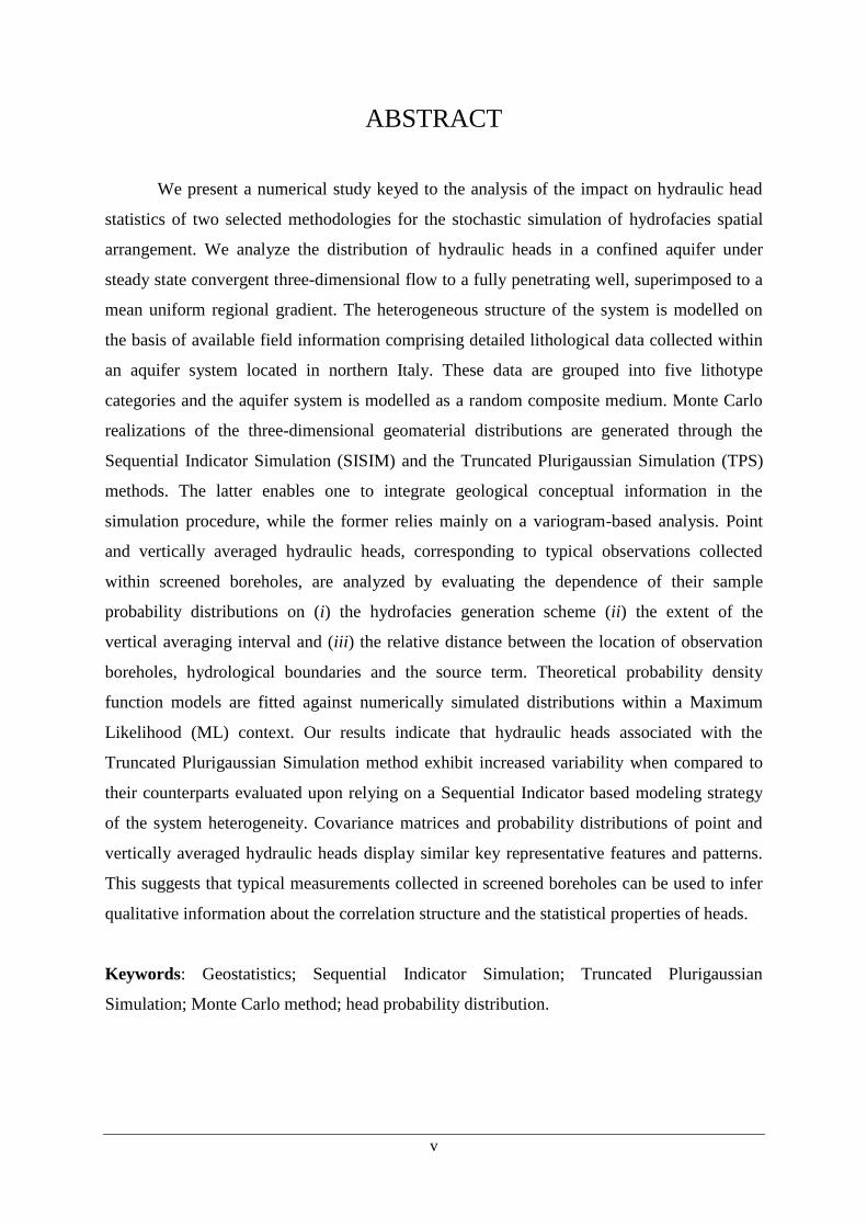
ABSTRACT
We present a numerical study keyed to the analysis of the impact on hydraulic head
statistics of two selected methodologies for the stochastic simulation of hydrofacies spatial
arrangement. We analyze the distribution of hydraulic heads in a confined aquifer under
steady state convergent three-dimensional flow to a fully penetrating well, superimposed to a
mean uniform regional gradient. The heterogeneous structure of the system is modelled on
the basis of available field information comprising detailed lithological data collected within
an aquifer system located in northern Italy. These data are grouped into five lithotype
categories and the aquifer system is modelled as a random composite medium. Monte Carlo
realizations of the three-dimensional geomaterial distributions are generated through the
Sequential Indicator Simulation (SISIM) and the Truncated Plurigaussian Simulation (TPS)
methods. The latter enables one to integrate geological conceptual information in the
simulation procedure, while the former relies mainly on a variogram-based analysis. Point
and vertically averaged hydraulic heads, corresponding to typical observations collected
within screened boreholes, are analyzed by evaluating the dependence of their sample
probability distributions on (i) the hydrofacies generation scheme (ii) the extent of the
vertical averaging interval and (iii) the relative distance between the location of observation
boreholes, hydrological boundaries and the source term. Theoretical probability density
function models are fitted against numerically simulated distributions within a Maximum
Likelihood (ML) context. Our results indicate that hydraulic heads associated with the
Truncated Plurigaussian Simulation method exhibit increased variability when compared to
their counterparts evaluated upon relying on a Sequential Indicator based modeling strategy
of the system heterogeneity. Covariance matrices and probability distributions of point and
vertically averaged hydraulic heads display similar key representative features and patterns.
This suggests that typical measurements collected in screened boreholes can be used to infer
qualitative information about the correlation structure and the statistical properties of heads.
Keywords: Geostatistics; Sequential Indicator Simulation; Truncated Plurigaussian
Simulation; Monte Carlo method; head probability distribution.
vi
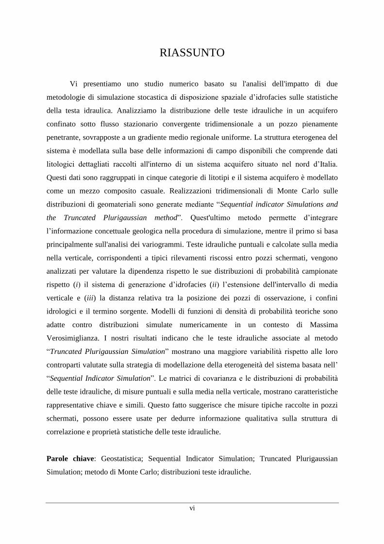
RIASSUNTO
Vi presentiamo uno studio numerico basato su l'analisi dell'impatto di due
metodologie di simulazione stocastica di disposizione spaziale d’idrofacies sulle statistiche
della testa idraulica. Analizziamo la distribuzione delle teste idrauliche in un acquifero
confinato sotto flusso stazionario convergente tridimensionale a un pozzo pienamente
penetrante, sovrapposte a un gradiente medio regionale uniforme. La struttura eterogenea del
sistema è modellata sulla base delle informazioni di campo disponibili che comprende dati
litologici dettagliati raccolti all'interno di un sistema acquifero situato nel nord d’Italia.
Questi dati sono raggruppati in cinque categorie di litotipi e il sistema acquifero è modellato
come un mezzo composito casuale. Realizzazioni tridimensionali di Monte Carlo sulle
distribuzioni di geomateriali sono generate mediante “Sequential indicator Simulations and
the Truncated Plurigaussian method”. Quest'ultimo metodo permette d’integrare
l’informazione concettuale geologica nella procedura di simulazione, mentre il primo si basa
principalmente sull'analisi dei variogrammi. Teste idrauliche puntuali e calcolate sulla media
nella verticale, corrispondenti a tipici rilevamenti riscossi entro pozzi schermati, vengono
analizzati per valutare la dipendenza rispetto le sue distribuzioni di probabilità campionate
rispetto (i) il sistema di generazione d’idrofacies (ii) l’estensione dell'intervallo di media
verticale e (iii) la distanza relativa tra la posizione dei pozzi di osservazione, i confini
idrologici e il termino sorgente. Modelli di funzioni di densità di probabilità teoriche sono
adatte contro distribuzioni simulate numericamente in un contesto di Massima
Verosimiglianza. I nostri risultati indicano che le teste idrauliche associate al metodo
“Truncated Plurigaussian Simulation” mostrano una maggiore variabilità rispetto alle loro
controparti valutate sulla strategia di modellazione della eterogeneità del sistema basata nell’
“Sequential Indicator Simulation”. Le matrici di covarianza e le distribuzioni di probabilità
delle teste idrauliche, di misure puntuali e sulla media nella verticale, mostrano caratteristiche
rappresentative chiave e simili. Questo fatto suggerisce che misure tipiche raccolte in pozzi
schermati, possono essere usate per dedurre informazione qualitativa sulla struttura di
correlazione e proprietà statistiche delle teste idrauliche.
Parole chiave: Geostatistica; Sequential Indicator Simulation; Truncated Plurigaussian
Simulation; metodo di Monte Carlo; distribuzioni teste idrauliche.

1
Index
1. INTRODUCTION ............................................................................................................ 4
1.1. Aims .......................................................................................................................................................... 4
1.2. Objectives ................................................................................................................................................. 5
1.3. Structure................................................................................................................................................... 6
1.4. Originality and principal outcome ......................................................................................................... 7
2. LITERATURE REVIEW ................................................................................................ 8
2.1. Geostatistical simulations...................................................................................................................... 11
2.2. Hydraulic head pdfs .............................................................................................................................. 13
3. CREMONA FIELD CASE STUDY .............................................................................. 16
3.1. Area under study ................................................................................................................................... 16
3.1.1. Location .......................................................................................................................................... 16
3.1.2. Previous studies .............................................................................................................................. 18
3.1.3. Hydrogeological structure ............................................................................................................... 19
3.1.4. Wells / piezometers ......................................................................................................................... 22
3.1.5. Springs ............................................................................................................................................ 24
3.2. Reference information database ........................................................................................................... 26
3.3. Regional vulnerabilities ......................................................................................................................... 30
3.4. Final remark .......................................................................................................................................... 30
4. METHODOLOGY ......................................................................................................... 31
4.1. Modifying the geological database ....................................................................................................... 31
4.2. Recalling geostatistical concepts ........................................................................................................... 33
4.3. Indicator variogram calculation ........................................................................................................... 34
4.4. SISIM vs TPS (and the geostatistical simulations) ............................................................................. 35
4.5. Flow field simulations using VMOD .................................................................................................... 39
4.6. Workflow for treating the output from the multi-realization scheme .............................................. 42
2
5. AQUIFER SYSTEM SIMULATIONS ......................................................................... 43
5.1. Modifying the geological database ....................................................................................................... 43
5.2. Variogram analysis and indicator variogram model fitting results .................................................. 46
5.3. Description of representative results ................................................................................................... 50
5.3.1. Qualitative analysis of heterogeneity’ reproduction for SISIM and TPS ....................................... 52
5.3.2. Statistical analysis of SISIM and TPS output volumetric proportions ............................................ 53
5.3.3. Variogram calculations from output simulations (SISIM and TPS) ............................................... 58
5.3.4. Sample LogK fields for mean (µ) and variance (σ2), from SISIM and TPS ................................... 60
6. FLOW FIELD SIMULATIONS ................................................................................... 63
6.1. Stating the problem: modeling details and procedure ....................................................................... 63
6.1.1. Numerical grid ................................................................................................................................ 64
6.1.2. Boundary conditions ....................................................................................................................... 66
6.2. N-S and W-E ensemble average drawdown maps .............................................................................. 67
6.3. Hydraulic heads’ variance and covariance maps for different degrees of vertical averaging ........ 71
6.4. Sample pdf estimation for point and vertically averaged hydraulic heads ...................................... 76
6.5. Sample pdf fitting procedure to Gaussian and α-stable models ........................................................ 80
7. DISCUSSION .................................................................................................................. 88
7.1. Practical applications ............................................................................................................................ 88
7.2. Objective and novelty ............................................................................................................................ 88
7.3. Indicator simulations ............................................................................................................................. 91
7.3.1. Comparison of SISIM and TPS results ........................................................................................... 92
7.3.2. Providing guidelines ....................................................................................................................... 93
7.3.3. Consequences of using SISIM and/or TPS ..................................................................................... 95
7.3.4. When should be used one or another? Both? .................................................................................. 97
7.4. Flow field simulations ............................................................................................................................ 99
7.4.1. Comparison of SISIM and TPS results ......................................................................................... 100
7.4.2. Providing guidelines ..................................................................................................................... 107
7.4.2.1. Vulnerability issues....................................................................................................................... 109
8. CONCLUSIONS ........................................................................................................... 110
8.1. Future work ......................................................................................................................................... 111
3
9. ANNEXES / APPENDIXES ........................................................................................ 114
9.1. Publications .......................................................................................................................................... 114
9.2. Dissemination activities ....................................................................................................................... 115
9.2.1. Conferences and workshops ......................................................................................................... 115
9.2.2. Posters at international conferences .............................................................................................. 115
9.2.3. Oral presentations ......................................................................................................................... 116
9.3. Appendix to Chapter 7 ........................................................................................................................ 117
10. REFERENCES .......................................................................................................... 121
Characterization of groundwater dynamics in response to forcing terms under uncertainty
4
1. Introduction
The current Ph.D. thesis has been developed under the umbrella of the European
Marie Curie ITN (Initial Training Network) IMVUL “Towards improved groundwater
vulnerability assessment”.
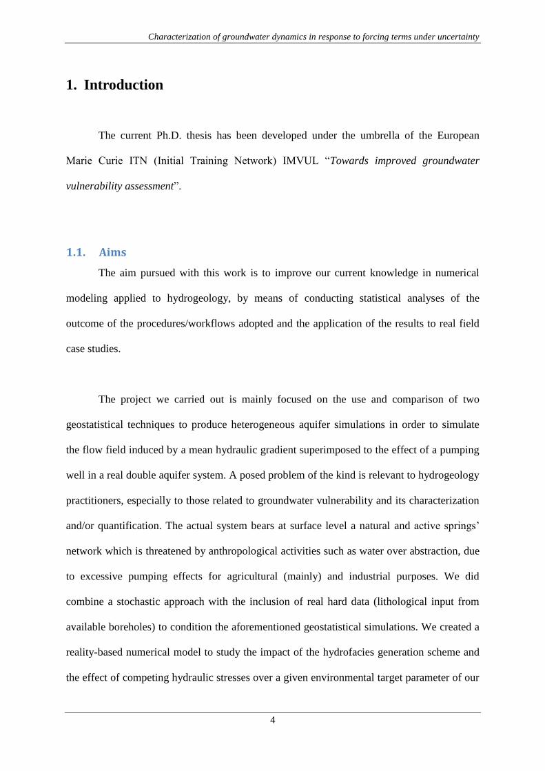
1.1. Aims
The aim pursued with this work is to improve our current knowledge in numerical
modeling applied to hydrogeology, by means of conducting statistical analyses of the
outcome of the procedures/workflows adopted and the application of the results to real field
case studies.
The project we carried out is mainly focused on the use and comparison of two
geostatistical techniques to produce heterogeneous aquifer simulations in order to simulate
the flow field induced by a mean hydraulic gradient superimposed to the effect of a pumping
well in a real double aquifer system. A posed problem of the kind is relevant to hydrogeology
practitioners, especially to those related to groundwater vulnerability and its characterization
and/or quantification. The actual system bears at surface level a natural and active springs’
network which is threatened by anthropological activities such as water over abstraction, due
to excessive pumping effects for agricultural (mainly) and industrial purposes. We did
combine a stochastic approach with the inclusion of real hard data (lithological input from
available boreholes) to condition the aforementioned geostatistical simulations. We created a
reality-based numerical model to study the impact of the hydrofacies generation scheme and
the effect of competing hydraulic stresses over a given environmental target parameter of our

Characterization of groundwater dynamics in response to forcing terms under uncertainty
5
choice: h (hydraulic heads). The output of a study of the kind we propose could be used to
guide setting thresholds or limits in water abstractions, in order to control hazardous
drawdowns that could lead to the drying up of a springs’ network fed by a confined aquifer.
1.2. Objectives
In this dissertation, we perform a numerical Monte Carlo (MC) study based on a
geological system whose heterogeneous structure mimics the one associated with an alluvial
aquifer system located in northern Italy (Cremona province, Regione Lombardia) where
abundant lithological and geological information are available. Our analysis considers a non-
uniform flow scenario due to the superimposition of a base uniform (in the mean) flow and
the action of a pumping well. Field-scale available lithological data are analyzed to
characterize prevalent lithotype categories and the associated geological contact rules. The
simulation domain is modeled as a composite medium with randomly distributed hydrofacies,
each associated with a given hydraulic conductivity. Collections of conditional Monte Carlo
realizations of the three-dimensional geomaterials distributions are generated by (i) a
classical indicator-based approach (Sequential Indicator simulations, SISIM) and (ii) the
Truncated Plurigaussian simulations (TPS) scheme, starting from available data which are
employed as conditioning information. Afterwards we performed a statistical analysis (in
terms of mean, variance, covariance function and probability distribution) of hydraulic heads
as a function of (i) location in the domain and (ii) methodology of geological reconstruction
of the system, highlighting the competing effect of the source term and boundary conditions.
Since typical head observations are collected within screened boreholes, we explore the
extent to which vertically averaging hydraulic heads can retain qualitative and quantitative
information on the statistical behavior of point-wise head values.

Characterization of groundwater dynamics in response to forcing terms under uncertainty
6
1.3. Structure
The dissertation is organized as follows. We do start framing our research revising the
previous scientific contributions by means of a review of the available literature in Chapter 2.
Chapter 3 is devoted to illustrate the reader with the current information database related to
the real field case study. There we describe the geological setup and present the previous
studies/surveys carried out in the area. We point out the relevance of the chosen area in terms
of groundwater vulnerability issues drawing the scenario where the numerical analysis is
meant to be applied for. A description of the available lithological database is performed.
Chapter 4 reports details about the methodology developed and employed. From modifying
the available borehole database in order to simplify the naturally high heterogeneity of the
hydrofacies system, through recalling some basic geostatistical concepts needed for our
study, we introduce the two widely used geostatistical approaches employed to conditionally
simulate (to hard data), in a MC framework, the large scale confined aquifer. We describe the
hydrofacies simulation stage and the flow field simulations performed by means of the
commonly used MODFLOW code. Finally we provide some guidelines on how we treated
the output at different stages to allow reproduction of the results, bringing light to the
procedure utilized to perform the posterior statistical analysis. Chapter 5 treats in detail the
hydrofacies simulations approach adopted in our study while Chapter 6 deals with the
description of the aquifer flow field simulations. A thorough discussion upon the obtained
results is performed in Chapter 7, both for the geostatistical reconstruction of the aquifer
system and the flow simulations. We end up with the major findings and conclusions, along
with future work and potential research tracks that can be pursued. Annexes / Appendixes
containing publications, dissemination activities and other extra material can be found at the
end of this work. Before its end we enclose a list with scientific references.
Characterization of groundwater dynamics in response to forcing terms under uncertainty
7
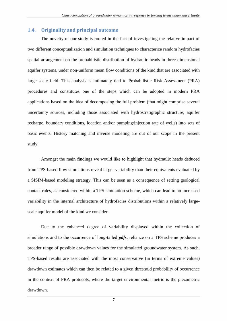
1.4. Originality and principal outcome
The novelty of our study is rooted in the fact of investigating the relative impact of
two different conceptualization and simulation techniques to characterize random hydrofacies
spatial arrangement on the probabilistic distribution of hydraulic heads in three-dimensional
aquifer systems, under non-uniform mean flow conditions of the kind that are associated with
large scale field. This analysis is intimately tied to Probabilistic Risk Assessment (PRA)
procedures and constitutes one of the steps which can be adopted in modern PRA
applications based on the idea of decomposing the full problem (that might comprise several
uncertainty sources, including those associated with hydrostratigraphic structure, aquifer
recharge, boundary conditions, location and/or pumping/injection rate of wells) into sets of
basic events. History matching and inverse modeling are out of our scope in the present
study.
Amongst the main findings we would like to highlight that hydraulic heads deduced
from TPS-based flow simulations reveal larger variability than their equivalents evaluated by
a SISIM-based modeling strategy. This can be seen as a consequence of setting geological
contact rules, as considered within a TPS simulation scheme, which can lead to an increased
variability in the internal architecture of hydrofacies distributions within a relatively large-
scale aquifer model of the kind we consider.
Due to the enhanced degree of variability displayed within the collection of
simulations and to the occurrence of long-tailed pdfs, reliance on a TPS scheme produces a
broader range of possible drawdown values for the simulated groundwater system. As such,
TPS-based results are associated with the most conservative (in terms of extreme values)
drawdown estimates which can then be related to a given threshold probability of occurrence
in the context of PRA protocols, where the target environmental metric is the piezometric
drawdown.

Characterization of groundwater dynamics in response to forcing terms under uncertainty
8
2. Literature review
Heterogeneity is embedded in practically all life systems at almost every scale. This
assumption also affects/includes geosciences and its related fields/disciplines. In particular
we are interested in characterizing the natural heterogeneity that exists in groundwater
systems, by means of Geostatistics and numerical simulations, specifically at a field scale.
This is one of our objectives in order to improve the current knowledge in numerical
modeling of water reservoirs and links to the more general aim of estimation and
quantification of groundwater vulnerability in real/natural systems.
We decided to employ widely used and well-known, both by academics and
practitioners, geostatistical and numerical tools to simulate a double aquifer system and its
associated flow field when a pumping well is acting as a sink/forcing term in the system. The
situation just described is compatible with actual field practices like water abstractions for
agricultural, industrial or drinking water purposes. These stresses are applied to natural
environments which react in turn, mostly having a negative impact on the available water
resources and the surrounding natural environments. Sometimes the aforementioned stresses
are pushed to certain limits that drive the system into a non-equilibrium state. Since these
activities cannot cease due to civil/industrial requirements, a compromise needs to be met in
order to protect the resources we are exploiting (and sometimes overexploiting).
What we propose is a stochastic approach conducted at a field scale, involving
geostatistical and numerical analyses, in order to compare two methodologies and the joint
information we can extract from their outcome. In other words, we compared two well-
established geostatistical methods that treat in a different way the heterogeneity embedded in
Characterization of groundwater dynamics in response to forcing terms under uncertainty
9
natural systems, and the impact of the geostatistical simulation on the posterior flow field
solution (and in particular, on the hydraulic heads). This allowed us estimating low order
moment statistics of calculated hydraulic heads in order to forecast which method introduces
more variability in the results and/or which method can be useful as a function of the context
under study (extreme values analysis, worst case scenario, etc.). From a practical point of
view, in stochastic hydrogeology, it is of great importance being able to put thresholds on
water abstractions that might lower local/regional hydraulic heads leading towards a real
menace to the available groundwater resources.
The present work is focused on the assessment of the impact on hydraulic head
statistics of two geostatistically-based methodologies for the stochastic simulation of the
spatial arrangement of hydrofacies in field scale aquifer systems. The relevance of an
appropriate characterization of the probability distribution of hydraulic heads is critical in the
context of Probabilistic Risk Assessment (PRA) procedures which are nowadays considered
as viable procedures to estimate the risk associated with catastrophic events in environmental
problems (Tartakovsky, 2013 and references therein). Application of PRA to actual settings
typically requires the estimate of the probability density function (pdf) of a target
Environmental Performance Metric (EPM, a terminology introduced by De Barros et al.,
2012).
The study of the relative impact of different conceptualization and simulation
techniques to represent random hydrofacies spatial arrangement on the probabilistic
distribution of hydraulic heads in three-dimensional aquifer systems under non-uniform mean
flow conditions of the kind that is associated with large scale field settings is still lacking. As
highlighted above, this analysis is tied to Probabilistic Risk Assessment procedures and
constitutes one of the steps which can be adopted in modern PRA applications based on the

Characterization of groundwater dynamics in response to forcing terms under uncertainty
10
idea of decomposing the full problem (that might comprise several uncertainty sources,
including those associated with hydrostratigraphic structure, aquifer recharge, boundary
conditions, location and/or pumping/injection rate of wells) into sets of basic events (e.g.,
Bolster et al., 2009; Jurado et al., 2012; Tartakovsky, 2013 and references therein).
Here we perform a numerical Monte Carlo study based on a geological system whose
heterogeneous structure mimics the one associated with an alluvial aquifer system located in
northern Italy, where abundant lithological and geological information are available. Our
analysis considers a non-uniform flow scenario due to the superimposition of a base uniform
(in the mean) flow and the action of a pumping well. Field-scale available lithological data
are analyzed to characterize prevalent lithotype categories and the associated geological
contact rules. The simulation domain is modeled as a composite medium with randomly
distributed hydrofacies, each associated with a given hydraulic conductivity. Collections of
conditional Monte Carlo realizations of the three-dimensional geomaterials distributions are
generated by (i) a classical indicator-based approach and (ii) the TPS scheme, starting from
available data which are employed as conditioning information. We present a statistical
analysis (in terms of mean, variance, covariance function and probability distribution) of
hydraulic heads as a function of (i) location in the domain and (ii) methodology of geological
reconstruction of the system, highlighting the competing effect of the source term and
boundary conditions. Since typical head observations are collected within screened boreholes,
we explore the extent to which vertically averaging hydraulic heads can retain qualitative and
quantitative information on the statistical behavior of point-wise head values.
Characterization of groundwater dynamics in response to forcing terms under uncertainty
11
2.1. Geostatistical simulations
Geostatistics can be roughly defined as the branch of Geology and/or Statistics that
deals with the study of phenomena that vary over the spatial dimension. It was developed
originally in the context of mining industry, to tackle problems that dealt with the spatial
prediction of mineral ore grades. Its general approach led afterwards to its vast application in
a wide range of settings across the geographical, geological, atmospheric, environmental, and
epidemiological sciences (among others). Geostatistics mainly provides a set of probabilistic
tools that help in understanding and modeling the spatial variability of a target variable of
interest, bearing in mind the main motivation of predicting unsampled values of the
aforementioned variable over areas/volumes where little/scarce information is provided. This
process is also (well-) known as interpolation. It is necessary to soar to the work of Daniel
Krige and other authors to find the origins of the discipline. They developed methods to
calculate/estimate gold and uranium reserves in the Witwatersrand, in South Africa, during
the decade of the 1950’s. Their ideas were extended and formalized during the 1960’s by the
French statistician Georges Matheron, who coined the term Geostatistics.
The selection of a model through which one can describe the natural heterogeneity of
a system is a key point in the analysis of the distribution of groundwater flow (and possibly
transport) variables. The model choice strongly depends on the scale of investigation. At the
large field scale, geological heterogeneity of sedimentary bodies can be represented and
modeled from information on depositional facies distributions. Statistical grid-based
sedimentary Facies Reconstruction and Modeling (FRM) methods can be employed to
provide consistent representations of facies distribution and are amenable to include
conditioning to hard and/or soft data. Falivene et al. (2007) provide an overview of the most
widely used deterministic and stochastic FRM methods, including pixel-based methods

Characterization of groundwater dynamics in response to forcing terms under uncertainty
12
termed as sequential indicator simulation (SISIM), transition probability schemes (e.g., T-
PROGS; Carle, 1999), multiple point simulation (Strebelle, 2002; Zhang et al., 2006; Wu et
al. 2008), truncated Gaussian simulation (TGS) and truncated plurigaussian simulation (TPS).
Sequential indicator algorithms are widespread geostatistical simulation techniques
that rely on indicator (co-) kriging. These have been applied to different datasets to study the
influence of the random distribution of aquifer sedimentological facies on target
environmental variables. In this context, Riva et al. (2006) present a synthetic numerical
Monte Carlo study aimed at analyzing the relative importance of uncertain facies architecture
and hydraulic attributes (hydraulic conductivity and porosity) on the probabilistic distribution
of three-dimensional well catchments and time-related capture zones. The authors base their
comparative study on a rich database comprising sedimentological and hydrogeological
information collected within a shallow alluvial aquifer system. Riva et al. (2008, 2010) adopt
the same methodology to interpret the results of a field tracer test performed in the same
setting. These authors consider different conceptual models to describe the system
heterogeneity, including scenarios where the facies distribution is random and modeled
through a SISIM-based technique and the hydraulic properties of each material are either
random or deterministically prescribed. Comparisons between the ability of different
geostatistical methods to reproduce key features of field-scale aquifer systems have been
published in the literature (e.g., Casar-González, 2001; Falivene et al., 2006; Scheibe and
Murray, 1998, Dell’Arciprete et al., 2012). Lee et al. (2007) performed a set of Monte Carlo
simulations to mimic a pumping test in an alluvial fan aquifer using the sequential Gaussian
simulation method and the transition probability indicator simulation. Emery (2004)
highlights limitations of SISIM upon examining the conditions under which a set of
realizations is consistent with the input parameters.
Characterization of groundwater dynamics in response to forcing terms under uncertainty
13
Truncated Gaussian simulation enables one to condition simulations on prior
information stemming from various sources while guaranteeing consistency between
variogram and cross-variogram of the variables considered. The possibility of using a
multiplicity of Gaussian functions to codify hydrofacies extends the potential of TGS and is
the cornerstone of TPS (Galli et al., 1994). Later on, Le Loc’h and Galli (1997) extended the
aforementioned reference. TPS allows taking into account complex transitions between
material types and simulating anisotropic distributions of lithotypes, whereas TGS explicitly
considers only sequentially ranked categories. The application of TPS usually aims at (i)
assessing the uncertainty associated with the location of the internal boundaries demarcating
geomaterials within the domain, and (ii) improving the geological constraints in the
characterization of quantitative attributes such as mineral ore grades. TPS is typically
employed to simulate geological domains in different contexts, including petroleum
reservoirs and mineral deposits, spatial arrangement of hydrofacies in aquifers, or soil types
at a catchment scale (e.g., Betzhold and Roth, 2000; Skvortsova et al., 2000; Fontaine and
Beucher, 2006; Galli et al., 2006; Emery et al., 2008; Dowd et al., 2007; Mariethoz et al.,
2009). More recently, a few publications brought open source codes/suites to use the TPS
workflow in standard personal computers (Dowd et al., 2003; Xu et al., 2006 and Emery,
2007). The routines are available as FORTRAN and MATLAB codes.
2.2. Hydraulic head pdfs
In the groundwater literature, the functional format of probability distributions of
solute travel/residence times, trajectories and concentrations has been extensively analyzed
during the last years (Fiorotto and Caroni, 2002; Bellin and Tonina, 2007; Riva et al., 2008,
2010; Schwede et al., 2008; Enzenhoefer et al., 2012 amongst others). On the other hand, less
attention has been devoted to study the probability distribution of hydraulic head (h) in
Characterization of groundwater dynamics in response to forcing terms under uncertainty
14
complex groundwater systems and under non-uniform (in the mean) flow conditions. These
settings are crucial for the study of the (negative) consequences arising from events
associated with the occurrence of h dropping below (or rising above) a given threshold.
These basic events are critical for various goal-oriented risk assessment practices including,
e.g., the protection of natural springs, ponds or the prevention of damages to underground
infrastructures. They all constitute core requirements in the planning of groundwater
abstraction procedures or during the designing of protection barriers. In this context,
estimates of first and second (conditional or unconditional) statistical moments of h have
been largely analyzed by means of analytical (e.g., Guadagnini et al., 2003; Riva and
Guadagnini, 2009 and references therein) or numerical (e.g., Guadagnini and Neuman,
1999b; Hernandez et al., 2006) methods for bounded randomly heterogeneous aquifers under
the action of pumping. Low-order (statistical) moments (i.e., mean and variance-covariance)
of hydraulic heads in unbounded and bounded domains under uniform (in the mean flow)
conditions have been investigated, amongst others, by: Dagan (1985), Rubin and Dagan
(1988, 1989), Ababou et al. (1989), Dagan (1989), Osnes (1995), Guadagnini and Neuman
(1999a, b). Even as these low-order moments have a considerable theoretical and practical
interest, they are not directly suitable to PRA protocols where the behavior of the tails of the
target variable distribution needs to be identified. This behavior can differ from the one
dictated by the classically assumed Gaussian or lognormal distributions and can be influenced
by the type of system heterogeneity, hydraulic boundaries and source/sink terms, as we
discuss in this work.
Jones (1990) observed the non-Gaussian shape of heads’ pdf close to pumping wells
in a two-dimensional confined aquifer where the transmissivity is lognormally distributed and
spatially correlated according to an exponential covariance model. Kunstmann and Kastens
Characterization of groundwater dynamics in response to forcing terms under uncertainty
15
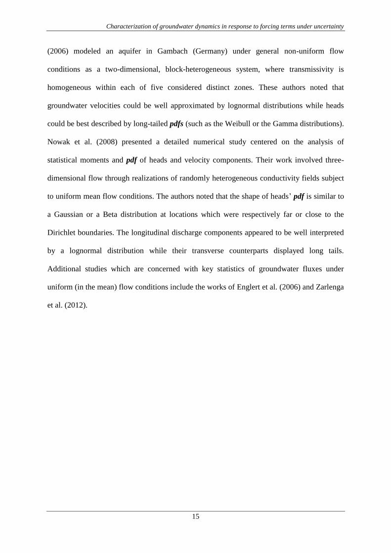
(2006) modeled an aquifer in Gambach (Germany) under general non-uniform flow
conditions as a two-dimensional, block-heterogeneous system, where transmissivity is
homogeneous within each of five considered distinct zones. These authors noted that
groundwater velocities could be well approximated by lognormal distributions while heads
could be best described by long-tailed pdfs (such as the Weibull or the Gamma distributions).
Nowak et al. (2008) presented a detailed numerical study centered on the analysis of
statistical moments and pdf of heads and velocity components. Their work involved three-
dimensional flow through realizations of randomly heterogeneous conductivity fields subject
to uniform mean flow conditions. The authors noted that the shape of heads’ pdf is similar to
a Gaussian or a Beta distribution at locations which were respectively far or close to the
Dirichlet boundaries. The longitudinal discharge components appeared to be well interpreted
by a lognormal distribution while their transverse counterparts displayed long tails.
Additional studies which are concerned with key statistics of groundwater fluxes under
uniform (in the mean) flow conditions include the works of Englert et al. (2006) and Zarlenga
et al. (2012).

Characterization of groundwater dynamics in response to forcing terms under uncertainty
16
3. Cremona field case study
In this section we describe the Cremona aquifer from a hydrogeological point of view.
3.1. Area under study
3.1.1. Location
The area subject of this study is the territory portion of the Pianura Padana valley
bounded to the west and south by the river Adda (which runs North-South) to Crotta d'Adda,
where it enters the river Po, and eastward from river Serio, which runs along the North-South
direction until Montodine, where it flows into the river Adda.
In the absence of a clear identification of a hydrogeological boundary, the
demarcation of the northern limit was evaluated in a manner consistent with other studies
conducted in the aforementioned region. In particular, it was adopted the same northern
boundary identified in a thesis project developed at the Politecnico di Milano by Rametta,
(2008). That is located along the northern boundary running parallel to the coordinate Gauss-
Boaga 5060000 North. The limits described above identify an area of approximately 785
km2. This system will be identified later in terms of “the large scale model”. Figure 3.1.1.1
displays a sketch with the area under study.
Characterization of groundwater dynamics in response to forcing terms under uncertainty
17
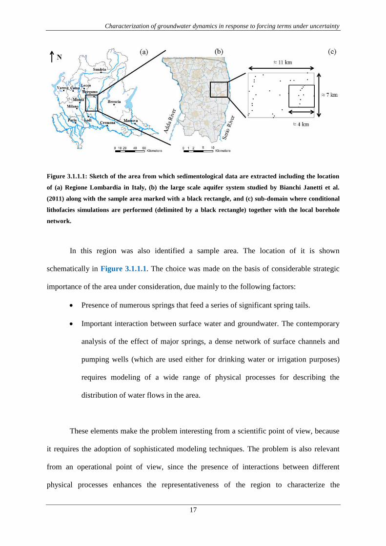
Figure 3.1.1.1: Sketch of the area from which sedimentological data are extracted including the location
of (a) Regione Lombardia in Italy, (b) the large scale aquifer system studied by Bianchi Janetti et al.
(2011) along with the sample area marked with a black rectangle, and (c) sub-domain where conditional
lithofacies simulations are performed (delimited by a black rectangle) together with the local borehole
network.
In this region was also identified a sample area. The location of it is shown
schematically in Figure 3.1.1.1. The choice was made on the basis of considerable strategic
importance of the area under consideration, due mainly to the following factors:
Presence of numerous springs that feed a series of significant spring tails.
Important interaction between surface water and groundwater. The contemporary
analysis of the effect of major springs, a dense network of surface channels and
pumping wells (which are used either for drinking water or irrigation purposes)
requires modeling of a wide range of physical processes for describing the
distribution of water flows in the area.
These elements make the problem interesting from a scientific point of view, because
it requires the adoption of sophisticated modeling techniques. The problem is also relevant
from an operational point of view, since the presence of interactions between different
physical processes enhances the representativeness of the region to characterize the
Characterization of groundwater dynamics in response to forcing terms under uncertainty
18
phenomena that takes place in the whole range of fountains that develops in the West (eastern
Pianura Padana).
3.1.2. Previous studies
Hydrogeological studies conducted by Maione et al. (1991) and Gandolfi et al. (2007)
investigated, respectively, the portion of the province of Bergamo in the south of the Alps
Orobie and the entire province of Cremona. These studies have provided an important source
of data and a valuable source of prior knowledge of the area investigated.
The area surveyed by Maione et al. (1991) is located between the rivers Adda and
Serio and bounded by the Alps and the northern outcrop line of fountains. The authors
proposed a geological model which identifies two distinct aquifers: a shallow phreatic aquifer
and a deep artesian aquifer, which flows beneath the surface without significant interaction
with the former.
The model proposed by Gandolfi et al. (2007) which covers the entire province of
Cremona, is bordered in the West by the river Adda, on the East by the Oglio river and in the
South by the river Po. In the North, since there is a lack of natural water boundary that can be
adopted as a closure model, was chosen the northern boundary along a line joining the rivers
Adda and Oglio at a distance of several kilometers North of the administrative boundary of
the province of Cremona. The conceptual model of the aquifer system shows a double system
of groundwater flow with:
A surface portion characterized generally by high transmissivity and large flow
values supported by the surface trade with the hydrographical network. Recharge
is due to infiltration from rainfall and water used for irrigation.

Characterization of groundwater dynamics in response to forcing terms under uncertainty
19
A deeper portion characterized by a complex succession of geological bodies with
different conductivities, which are essentially governed by the flow of water
withdrawals for drinking water supply. Its flow values are well below the ones
transiting the upper portion.
3.1.3. Hydrogeological structure
The available literature research and the collection of stratigraphic data were initially
extended to the provinces of Bergamo and Cremona. At a later stage, attention was focused
on the portion of land bounded by the paths of the rivers Adda and Serio.
The preliminary conceptual geological model of the area under investigation was
constructed on the basis of the following information and documents:
Maione et al. (1991): drawn from the study were 218 stratigraphic columns
located in the provinces of Bergamo and Cremona and 15 reconstructed
lithostratigraphic sections.
Provincia di Cremona – Atlante Ambientale: in the study were used 464
stratigraphic columns located within the province of Cremona.
Consorzio della Media Pianura Bergamasca (CMPB): we used 14 stratigraphic
columns.
Beretta et al. (1992): the study contains 29 reconstructed lithostratigraphic
sections from the province of Cremona.
The analysis of the sections can schematically identify, within the territory examined,
the presence of two overlapping aquifers within the Quaternary alluvial sequence of the
Padano sedimentary basin filling. This fact allows considering two different aquifers.
Characterization of groundwater dynamics in response to forcing terms under uncertainty
20
Phreatic aquifer. It is located in the coarse clastic deposits ranging between the
ground level and a clay level that is characterized by certain continuity at the investigation
scale. The roof of the body with low hydraulic conductivity, named by Maione et al. (1991)
“A horizon”, coincides with the clay level in the high plain which is present in the most
superficial fluvio-glacial Valtellina complex (which separates the polygenic strain from the
underlying calcareous strain). In the lowlands the delineation of the A horizon is more
uncertain. In general it is represented by a clay layer being within the same alluvial deposit,
following the criteria of Maione et al. (1991).
The superficial thickness consists of thick clastic continental deposits belonging to
different sedimentary cycles that appertain to diverse geological periods. Nevertheless, they
display a lateral continuity between them in terms of the hydraulic conductivity parameter.
Within these, stand out the following:
Polygenic conglomerate (fluvio-glacial Mindel) in the high plains.
Fluvio-glacial gravels and sands (RISS-Wurm) that form the lowlands and the
filling of the erosion furrows in the polygenic conglomerate.
Recent alluvial gravels and sands deposited by rivers that cross the plain.
In the northern line of Canonica d'Adda - Ghisalba prevail the conglomeratic deposits,
while in the southern portion dominate loose gravel and sand deposits. Within the aquifer
thickness are intercalated layers of clay with variable planar/lateral continuity. Due to this
fact, the aquifer may shift from ground conditions to local conditions of semi-confinement.
The thickness of this aquifer ranges from 40 m to 80 m, along the main anisotropic direction
of the system (North-South).
Characterization of groundwater dynamics in response to forcing terms under uncertainty
21
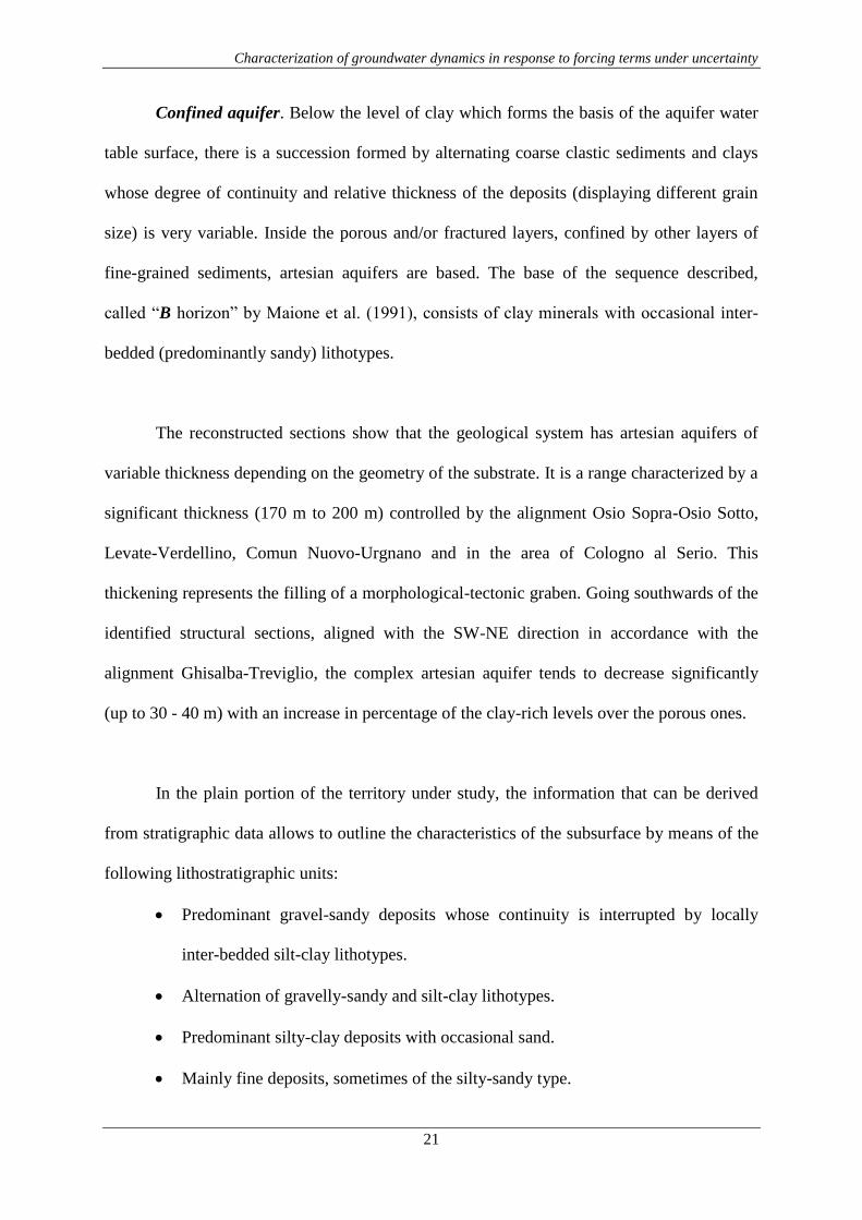
Confined aquifer. Below the level of clay which forms the basis of the aquifer water
table surface, there is a succession formed by alternating coarse clastic sediments and clays
whose degree of continuity and relative thickness of the deposits (displaying different grain
size) is very variable. Inside the porous and/or fractured layers, confined by other layers of
fine-grained sediments, artesian aquifers are based. The base of the sequence described,
called “B horizon” by Maione et al. (1991), consists of clay minerals with occasional inter-
bedded (predominantly sandy) lithotypes.
The reconstructed sections show that the geological system has artesian aquifers of
variable thickness depending on the geometry of the substrate. It is a range characterized by a
significant thickness (170 m to 200 m) controlled by the alignment Osio Sopra-Osio Sotto,
Levate-Verdellino, Comun Nuovo-Urgnano and in the area of Cologno al Serio. This
thickening represents the filling of a morphological-tectonic graben. Going southwards of the
identified structural sections, aligned with the SW-NE direction in accordance with the
alignment Ghisalba-Treviglio, the complex artesian aquifer tends to decrease significantly
(up to 30 - 40 m) with an increase in percentage of the clay-rich levels over the porous ones.
In the plain portion of the territory under study, the information that can be derived
from stratigraphic data allows to outline the characteristics of the subsurface by means of the
following lithostratigraphic units:
Predominant gravel-sandy deposits whose continuity is interrupted by locally
inter-bedded silt-clay lithotypes.
Alternation of gravelly-sandy and silt-clay lithotypes.
Predominant silty-clay deposits with occasional sand.
Mainly fine deposits, sometimes of the silty-sandy type.

Characterization of groundwater dynamics in response to forcing terms under uncertainty
22
3.1.4. Wells / piezometers
Information concerning the presence of wells/piezometers comes from the following
sources:
Regione Lombardia: Programma di Tutela e Uso delle Acque – PTUA.
Agenzia Regionale per la Protezione dell’Ambiente Lombardia - ARPA
Lombardia.
Consorzio di Bonifica della Media Pianura Bergamasca – CMPB.
Piezometric monitoring of the aquifer system in the region under consideration, can
be done using information from a set of 761 observation wells. It is worthy to point out that a
number of wells outside the large-scale model area were taken into account. This choice aims
at achieving greater consistency in order to track the reference piezometric maps, particularly
on the rivers which shape the limits of the superficial area influenced by the groundwater
flow model.
Information on the measurements of the land surface at the individual wells is
associated by means of using heterogeneous techniques. Among them, are included:
GPS measurements.
Interpolation from the base of the Regional Technical Cartography.
Topographic lines.
Unfortunately, it was not possible to trace the detailed description of the origin of
these values for each well. A first empirical test of the reliability of the allowances provided,
was determined by estimating the values of the land surface at the wells of interest from the
Digital Elevation Model DTM40.

Characterization of groundwater dynamics in response to forcing terms under uncertainty
23
The reliability of the data reported is of fundamental importance for a proper
definition of the piezometric level in the region. In fact, the measure monitored at all points
of observation is not the piezometric level, but rather the depth to the water table with respect
to the ground level. The piezometric level has been rebuilt, for each well/piezometer, as the
difference between the values of water table depth and the land surface.
The water table depth data from ARPA, registered monthly or bimonthly, covers a
time span between 1999 and 2006, while the database provided by the CMPB covers a longer
period which goes from 1989 to 2007. The measurement campaigns conducted by CMPB are
carried monthly or every two months. The water table depth data recorded by the Politecnico
di Milano (and reported within the PTUA) refers to three different surveys conducted in April
1994, November 1996 and March 2003.
Figure 3.1.4.1: Location of the wells in which the piezometric level is currently monitored (Guadagnini, L.
et al., 2008).
Characterization of groundwater dynamics in response to forcing terms under uncertainty
24
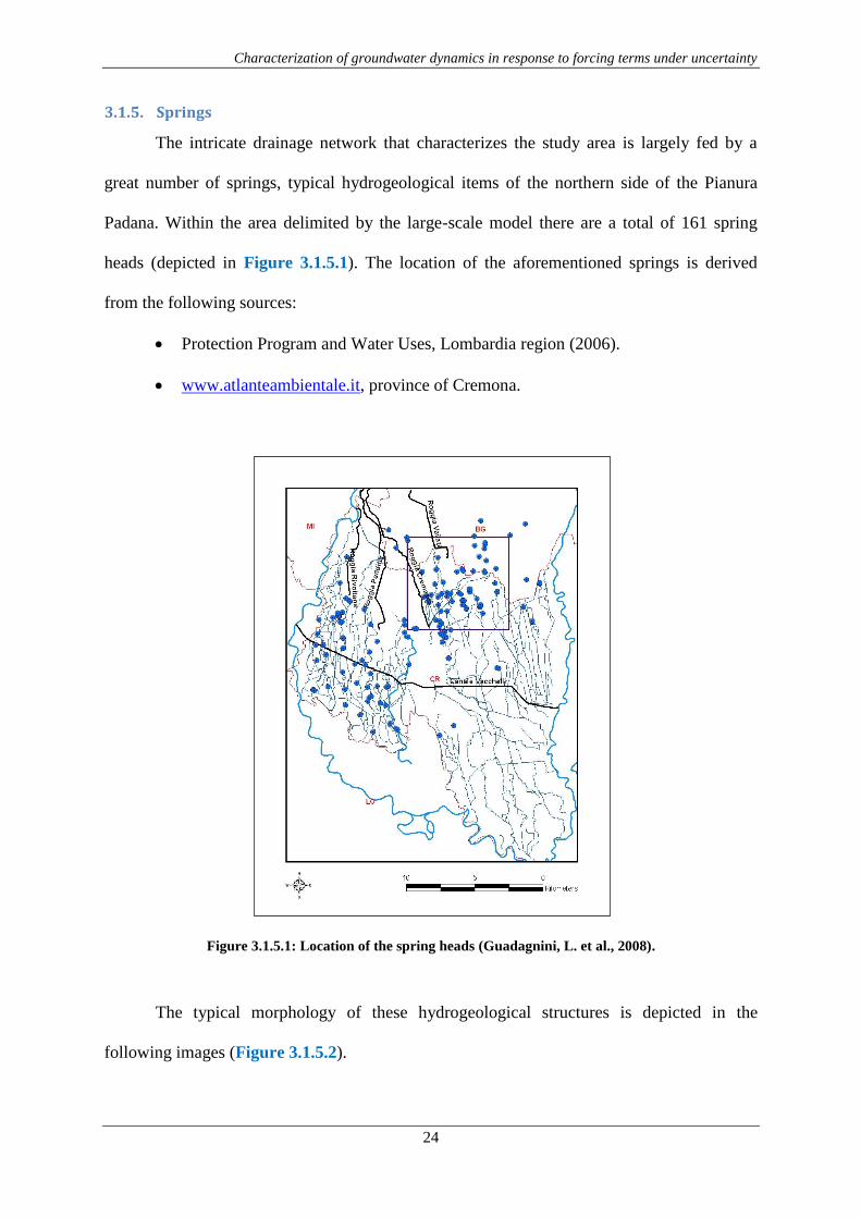
3.1.5. Springs
The intricate drainage network that characterizes the study area is largely fed by a
great number of springs, typical hydrogeological items of the northern side of the Pianura
Padana. Within the area delimited by the large-scale model there are a total of 161 spring
heads (depicted in Figure 3.1.5.1). The location of the aforementioned springs is derived
from the following sources:
Protection Program and Water Uses, Lombardia region (2006).
www.atlanteambientale.it, province of Cremona.
Figure 3.1.5.1: Location of the spring heads (Guadagnini, L. et al., 2008).
The typical morphology of these hydrogeological structures is depicted in the
following images (Figure 3.1.5.2).

Characterization of groundwater dynamics in response to forcing terms under uncertainty
25
While the two top pictures represent the typical planar section (top left) and vertical
cross-section (top right) of a spring, the bottom diagram illustrates the Pianura Padana system
from the highest area located in the North (Alps) to its distal zones. It can be noted here that,
as it is observable through our borehole database, exists a transition from coarser materials in
the northern boundary towards finer materials (when we approach the distal parts of the
alluvial system).
Figure 3.1.5.2 : Source: http://www.comune.capralba.gov.it/parco/territorio/fascia/index.aspx#/-1/,
http://www.cooperativadelsole.it/?p=446.

Characterization of groundwater dynamics in response to forcing terms under uncertainty
26
3.2. Reference information database
Implementing a flow model within a real aquifer system requires the structuring of an
information database that should contain a complete set of data necessary to understand, with
the greatest degree of detail possible, the geological architecture of the porous medium and
the hydrological processes that govern the flow field in the area under study. This database
should be structured in an organic and functional way, to:
Allow rapid access to the information of interest.
Ensure the ability to update quickly and effectively the data collection.
Guarantee the ability to interact with the mathematically formulated model.
A rough outline that could describe how the reference information database was
implemented can be divided into the following stages:
Collection of raw data from the different agencies responsible for monitoring the
quantities of interest.
Data selection for the region studied.
Analysis and processing of data in order to evaluate its significance at different
temporal and spatial scales.
Structuring the reference information base.
In Table 3.2.1 we present an extract of the already re-worked lithological database.
The information contained in the table below is compartmented in columns displaying,
amongst other fields: the well code (corresponding to the original database and map vertical
cross-sections); the three-dimensional UTM coordinates; identified strata thickness; its
relative depth expressed in m.a.s.l (meters above sea level); the detailed lithological
description and its indicator category.

Characterization of groundwater dynamics in response to forcing terms under uncertainty
27
Table 3.2.1: This database sample displays the rich geological data record build up aiming to obtain the necessary hard data for our simulation phase process, i.e.
the variogram analysis and the a posteriori geostatistical (conditional) simulations.
Codice X (m) Y (m) Z (m) Quota
(m.s.l.m)
Livello
stratigrafico
Spessore
(m)
Profondita
(m) Descrizione Dettagliata L1 L2 L3 Categoria
min 1534718.60 5036420.00 105.00 -123.69 --- 0.30 0.50 --- --- --- --- ---
max 1557725.54 5064758.56 270.00 270.00 --- 145.51 305.22 --- --- --- --- ---
37 1539941.32 5054573.75 222.00 222.00 1 2.7 2.7 Argilla e Limo A L --- 1
37 1539941.32 5054573.75 222.00 191.50 2 30.5 33.2 Ghiaia G --- --- 3
37 1539941.32 5054573.75 222.00 159.30 3 32.2 65.4 Conglomerato (Ghiaia Cementata) C --- --- 4
37 1539941.32 5054573.75 222.00 157.70 4 1.6 67 Ghiaia G --- --- 3
37 1539941.32 5054573.75 222.00 152.20 5 5.5 72.5 Conglomerato (Ghiaia Cementata) c fess. --- --- 5
37 1539941.32 5054573.75 222.00 150.90 6 1.3 73.8 Argilla e Limo A L --- 1
37 1539941.32 5054573.75 222.00 145.90 7 5 78.8 Conglomerato (Ghiaia Cementata) C --- --- 4
37 1539941.32 5054573.75 222.00 144.40 8 1.5 80.3 Argilla e Limo A L --- 1
37 1539941.32 5054573.75 222.00 137.40 9 7 87.3 Conglomerato (Ghiaia Cementata) C --- --- 4
37 1539941.32 5054573.75 222.00 132.90 10 4.5 91.8 Ghiaia G --- --- 3
37 1539941.32 5054573.75 222.00 125.30 11 7.6 99.4 Conglomerato (Ghiaia Cementata) c fess. --- --- 5
37 1539941.32 5054573.75 222.00 121.00 12 4.3 103.7 Argilla e Limo A L --- 1
37 1539941.32 5054573.75 222.00 118.90 13 2.1 105.8 Ghiaia G --- --- 3
37 1539941.32 5054573.75 222.00 113.90 14 5 110.8 Argilla e Limo A L --- 1

Characterization of groundwater dynamics in response to forcing terms under uncertainty
28
The total drilled depth information used in the area under study is slightly over 13.5
km (data belongs to the CMPB). For our purpose of quantifying the existing volumetric
proportions of the five re-classified lithotypes, and therefore finding a hint to establish the
final indicator values, we used the information coming from a bulk set of 144 wells. We
chose to keep constant the indicator volumetric proportions across the three-dimensional
space. We know that it is not a 100% realistic assumption but it helps to keep simpler, yet
valid, the problem under analysis.
We did carry a statistical analysis over some key features including the ones presented
in Table 3.2.2, in order to bring light to the modeling problem and be able to find proper
constraints for solving the geostatistical and the flow field simulations. For instance, knowing
the minimum well depth, its maximum and the mean, allowed us to set the boundaries in the
vertical direction for our numerical domain. We used, for our numerical simulations, the
vertical geological cross-sections along the N-S direction (namely S3, S4 and S5) as detailed
in the study from Guadagnini, L. et al. (2008). Along the W-E direction we used the S10 and
S11. The total borehole depth used as conditioning data adds up to almost 3.6 km, i.e. a
whole set of 35 wells. The minimum thickness recorded in the borehole dataset is 0.5 meters.
We did use this information to further discretize our remaining hard data.
Well depth [m] F1 vol.
(%)
F2 vol.
(%)
F3 vol.
(%)
F4 vol.
(%)
F5 vol.
(%)
TOTAL
(%)
3557.30 43.62 1.75 22.31 21.23 11.08 100.00
F1 F2 F3 F4 F5
min thickness [m] 0.50 1.53 0.50 0.50 1.00
MAX thickness [m] 59.03 19.98 39.11 46.77 128.83
Table 3.2.2: The top table displays the total drilled depth used to condition the numerical simulations and
estimate the volumetric facies proportions (kept constant across the full domain). The bottom table shows
the minimum and maximum thicknesses for every hydrofacies expressed in meters [m].

Characterization of groundwater dynamics in response to forcing terms under uncertainty
29
Table 3.2.3: The top left table represent the main lithotype classes found in the sample area under study, while the bottom left table displays the re-categorized
hydrofacies and the original categories that were included in each one. The top right table is presented to show a key finding that helped to establish the lithotype
rule for the Truncated Plurigaussian simulations. There we illustrate (in percentage values) the existing 456 transitions between the different geomaterials. This has
nothing to do with probability transitions. We wanted to investigate qualitatively and quantify the amount of times a facies appears next to the other remaining
facies.
LEGEND A+G argilla + ghiaia
A+L argilla + limo
A+F argilla + fossili
Asup. argilla superficiale
A+Lt argilla + limo + turba
C Conglomerate
Cf Conglomerate fessurato
G ghiaia
G+A ghiaia + argilla
S sabbia
Sc sabbia cementata
AR arenaria
T terreno
TOTAL
F1-F1 F1-F2 F1-F3 F1-F4 F1-F5
Transitions
10.53 1.97 22.37 26.10 11.62
456.00
F2-F2 F2-F3 F2-F4 F2-F5
Check (%)
0.00 1.10 0.66 0.00
100.00
F3-F3 F3-F4 F3-F5
1.32 14.91 3.51
F4-F4 F4-F5
2.19 3.51
F5-F5
0.22
F1 A+G, G+A, A+L, A+F, A+Lt, Asup, T
F2 S
F3 G
F4 C, AR, Sc
F5 Cf
Characterization of groundwater dynamics in response to forcing terms under uncertainty
30
3.3. Regional vulnerabilities
In the Cremona region the pollutants are not only the most worrying issue. Thanks to
the springs’ existence, a rich environment is developed on the ground surface. All the
activities that take place surrounding the springs’ area commit an overexploitation of the
aquifers in the zone under study. We refer mainly to agricultural practices, water pumping for
drinking purposes and industrial use, etc. Those actions produce non-equilibrium in the
system, provoking the decrease in the water level in the springs and their influence zone.
3.4. Final remark
We would like to point out some choices that we made at this stage and that affect the
latter steps of our research.
The restructured geological database containing the borehole information from
different sources allowed us to estimate the volumetric proportions of the final five regrouped
hydrofacies. Not only that, we could infer the crucial lithotype rule needed to run the
Truncated Plurigaussian simulations scheme. In addition, we determined (after consulting
surface lithological maps corresponding to the area under study) the main anisotropy
directions (along the N-S, W-E and vertical) and characteristic lengths of the geological
structures. As in the vast majority of studies of this kind, our available vertical hard data
resolution is much higher than its horizontal counterpart.
We decided to reduce the complex heterogeneity embedded in our natural
groundwater system by means of reclassifying the existent lithotypes into five
hydrogeologically meaningful hydrofacies. We chose to keep the problem simple by setting
stationary hydraulic conductivity values in the aforementioned indicator lithotypes.
Characterization of groundwater dynamics in response to forcing terms under uncertainty
31
4. Methodology
In the following we focus on the workflow we employed to pursue the goals stated in
the introduction of this dissertation.
4.1. Modifying the geological database
We introduced the actual geological database in Chapter 3, in order to show where the
conditioning data for our geostatistical simulations comes from. As previously stated we got a
few tenths of borehole records that gave us a hint of the inherent highly heterogeneous nature
of the geological materials found in the area under study. To be able to tackle this extra
(natural) complexity in an efficient computational way, and in order to get results in a limited
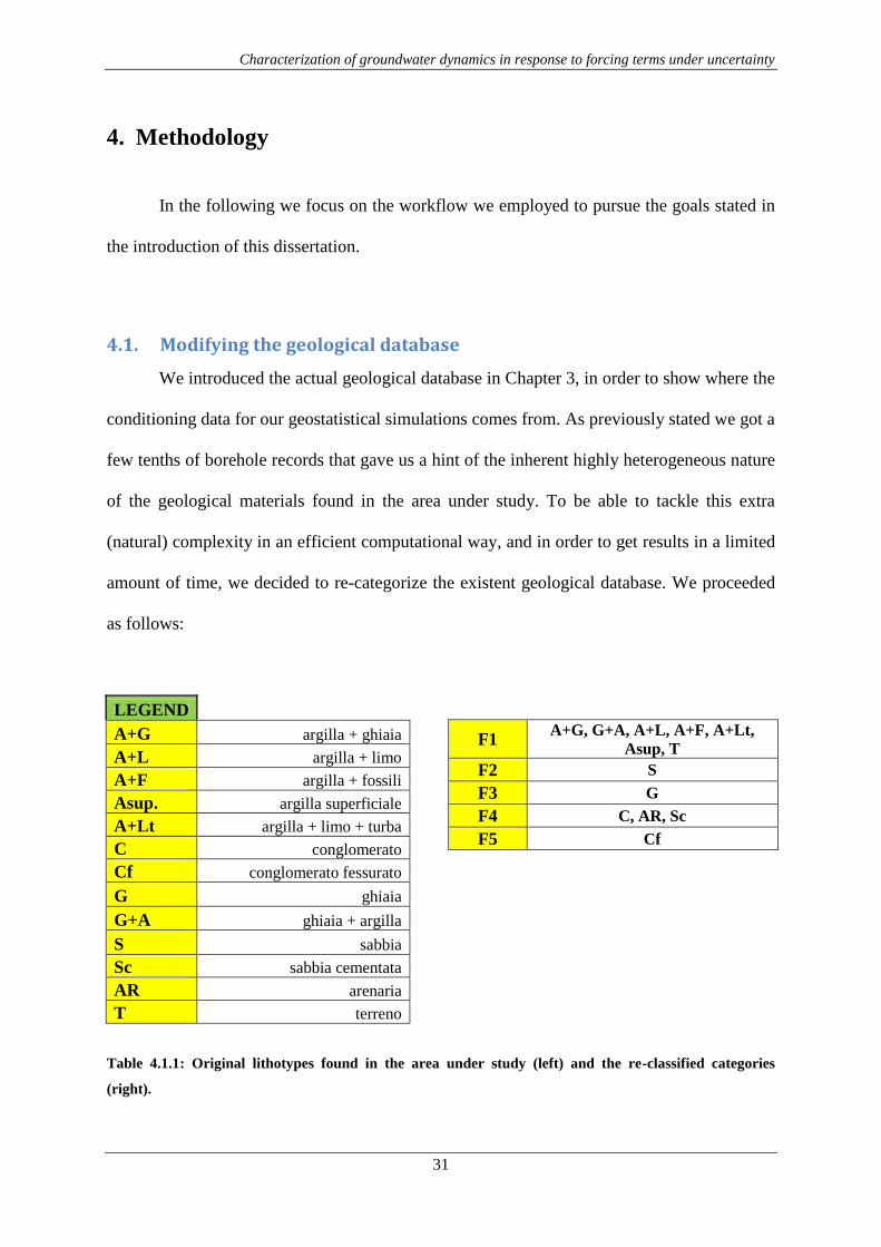
amount of time, we decided to re-categorize the existent geological database. We proceeded
as follows:
LEGEND A+G argilla + ghiaia
A+L argilla + limo
A+F argilla + fossili
Asup. argilla superficiale
A+Lt argilla + limo + turba
C conglomerato
Cf conglomerato fessurato
G ghiaia
G+A ghiaia + argilla
S sabbia
Sc sabbia cementata
AR arenaria
T terreno
Table 4.1.1: Original lithotypes found in the area under study (left) and the re-classified categories
(right).
F1 A+G, G+A, A+L, A+F, A+Lt,
Asup, T
F2 S
F3 G
F4 C, AR, Sc
F5 Cf

Characterization of groundwater dynamics in response to forcing terms under uncertainty
32
Therefore, by reducing the original lithological classes resulting from previous
surveys, we simplified the original problem and improved its computational tractability (in
terms of computing effort and time). The new categories or indicators were described as:
F1: fine materials.
F2: sands.
F3: gravels.
F4: conglomerates.
F5: fractured conglomerates.
As a way of computing the final volumetric proportions for each indicator, to be used
as an input in the geostatistical simulations, we took the newly reclassified values for the
different vertical (N-S and W-E) cross-sections and computed the corresponding percentages.
The results were the following:
Well depth [m] F1 [%] F2 [%] F3 [%] F4 [%] F5 [%] TOTAL [%]
3557.30 43.62 1.75 22.31 21.23 11.08 100.00
Table 4.1.2: Total borehole depth and estimated volumetric proportions from hard data source.
Initially we were tempted to remove the geomaterial indicator F2 (corresponding to
the sandy materials found in the system) due to its low contribution to the final volumetric
proportions percentage. Finally we decided to keep it as it was and analyze the impact on the
final geostatistical simulations. By keeping the hydrofacies class F2 not only we preserved in
a better way the original heterogeneity inherent to the double aquifer groundwater system, but
we were able to study the impact on the flow field simulations of a less representative facies.
This was possible because we decided to embed into every geomaterial category a steady
value of the hydraulic conductivity (K) for each indicator class, i.e. a constant (in time) value
of K.
Characterization of groundwater dynamics in response to forcing terms under uncertainty
33
We do contemplate the possibility of carrying on with the idea of suppressing the F2
hydrofacies in future studies, derived from the current research project.
4.2. Recalling geostatistical concepts
There exist various basic manuals about Geostatistics either for beginners and
practitioners in industry not familiar with the field (Clark, 1979), being mainly focused on the
mining industry. Kitanidis (1997) presents an introduction to Geostatistics along with some
applications in hydrogeology. “An introduction to applied Geostatistics” is probably the most
complete of those references (Isaaks and Srivastava, 1990).
Here we are not interested in delivering a complete geostatistical introduction, since
they already exist, but we would rather make explicit which concepts derived/coming from
Geostatistics we used for our research work. We used the term Geostatistics in the European
sense of the “Theory of the Regionalized Variables” developed by G. Matheron and co-
workers at Fontainebleau (1970’s). We made use of the simplest function that characterizes
any geostatistical study: the semivariogram. The definition of a semivariogram (γ) arises out
of the notion of continuity and relationship due to position. It is a graph (and/or formula)
describing the expected difference in value between pairs of samples (bearing a target
property of interest) with a given relative orientation. In the following we present its
mathematical expression:
γ
Where n are the sample pairs, g are the functions (properties under study) and h is the
fixed distance between the sampled positions. In our study we mostly dealt with vertical and
horizontal (omni-directional) indicator semivariograms computed from the available
conditioning indicator data.
Characterization of groundwater dynamics in response to forcing terms under uncertainty
34
4.3. Indicator variogram calculation
Before going through calculating the indicator variograms, we did need to generate
further conditioning data by refining (along the vertical direction) the available indicator
values. The information contained in the geological database spreadsheet, as usual in
borehole/core interpretation, made explicit where the appearance of a given lithotype
started/ended. We performed that a priori step in seeking an improvement of the subsequent
semivariogram analysis by introducing further more points in the variogram estimation. In
order to achieve this, we used an existing in-house built FORTRAN routine (named STRAT).
The aforementioned routine performed a data refinement along the vertical by, namely,
replicating the available data points every 0.5 meters (when necessary). That generated quite
a decent amount of conditioning data, sufficient to accept as valid the posterior results. In any
case it is worthy to note that as in almost geostatistical study, the information/resolution
obtained along the vertical direction was much higher than that along the horizontal plane.
This fact will inevitably condition our results but it is unavoidable from a technical point of
view, since it depends on the available data that we have used from previous field
studies/surveys. This is a common drawback faced by practitioners of all kind, but does not
invalidate the results obtained as long as it is recognized and accepted as a limitation of the
approach. In fact, this might lead to inaccurate results, introducing further uncertainty on the
final outcome.
For the statistical analysis that we wanted to carry out we needed to compute the
vertical and horizontal indicator semivariograms. That was made with the purpose of
estimating the ranges (and correlation lengths) of the hydrofacies semivariogram functions.
The resulting variogram ranges estimated at this step will act as input information for the
geostatistical simulations along with the volumetric proportions estimated previously. We
Characterization of groundwater dynamics in response to forcing terms under uncertainty
35
departed from our modified (extended) indicator conditioning dataset. We did use the
available computational tools provided for this purpose by the GSLIB manual (program
gamv, Deutsch and Journel, 1997). We did perform various types of variogram estimations
(mainly omni-directional and along the main anisotropy directions). Those calculations were
supported by the available geological information coming from previous studies and
superficial lithological maps. We found and determined that the main anisotropy directions
were along the N-S, W-E and the vertical direction. Finally we only considered, for posterior
fitting with an exponential variogram model, horizontal omni-directional and vertical
variograms.
An exponential semivariogram model was chosen (after performing a RSME analysis)
for fitting the directional semivariograms. For the purpose of this rather simple data treatment
(even though the dataset was pretty vast) and its statistical analysis, we employed common
available software packages (such as text and spreadsheet editors).
4.4. SISIM vs TPS (and the geostatistical simulations)
Among the vast range of FRM methods, following the classification in Falivene et al.
(2007), we decided to employ 2 different well-known and widely-spread geostatistical
indicator pixel-based methods. Those allowed us to compare the effect of the embedded
geological heterogeneity in the simulations and the posterior effect on the hydraulic head
pdfs, after solving the flow field problem in a multi-realization context. Pixel-based methods
work assigning a facies to grid cells according to the facies occurrence pdf, which is
computed for each grid cell. These methods allow direct conditioning by hard and/or soft
data. Categorical or indicator methods are based on transforming each facies category to a
new property, defined as the occurrence probability of the facies, and building the pdf at each
Characterization of groundwater dynamics in response to forcing terms under uncertainty
36
grid cell as the combination of the reconstruction or modeling of these new properties (e.g.
Journel and Alabert, 1989).
A number N = 1000 of three-dimensional realizations of hydrofacies distributions
were generated with TPS and SISIM schemes. Indicator-based conditional simulations are
performed via the software SISIM (Deutsch and Journel, 1997). TPS simulations are based
on the algorithms and codes presented by Xu et al. (2006) and Emery (2007). This number
has been found sufficient to support the validity/correctness of our analyses/work (results
regarding this can be found in Chapter 5). For the purpose of our analysis and for reason
related to computational costs, the numerical simulations are performed within a model
domain whose extent corresponds to the sub-domain identified in Figure 3.1.1.1. The
estimated computational effort, in terms of time has been approximately 2 weeks.
At this point we would like to emphasize that we carried out our simulations at a field
scale, since the available borehole database allowed for this kind of analysis. The lithological
and geological information available in this region were employed as conditioning data for
our aquifer system model. The Cartesian grid adopted for the hydrofacies simulations
comprises 74 × 86 elements, respectively along the N–S (y) and W–E (x) directions. The grid
spacing is set to Δx Δy = 50 m, resulting in a simulation domain with a planar extent of
3700 × 4300 m2. Since one of the objectives of this study is to analyze the way the vertical
variability of hydraulic heads is impacted by facies distribution, boundary conditions and/or
source terms without considering the effect of the particular geometry of the bottom of the
aquifer, we adopt in the following a constant thickness B = 100 m which is representative of
an average width of the system in the area. We discretize B into 50 layers of uniform
thickness Δz = 2 m for the purpose of our computations. Therefore the total amount of nodes
was 74 × 86 × 51, adding up to a total of 324,564 cells.

Characterization of groundwater dynamics in response to forcing terms under uncertainty
37
We decided to use SISIM (in its SGeMS implemented version) in first instance since
it is a common geostatistical tool among practitioners and academics, due to its:
Reliability and robustness.
Easy implementation.
Low computing requirements in terms of time and equipment.
We did use 5 categories with its computed volumetric proportions obtained from the
available conditioning hard data (see point 4.1 for further details). We opted for using a Full
IK option since we had information and estimated indicator variograms for every single
facies (horizontal omni-directional and vertical). Details of the estimated empirical
semivariograms can be found in Chapter 5.
We then chose to use the TPS approach. As stated previously, this is an extended
version of the Truncated Gaussian method. The main difference with respect to SISIM lies in
the lithotype rule. By means of this tool we are given the chance of including further
geological information from our area under study, constraining which contacts are allowed
between the different hydrofacies. This restriction implies a higher degree of realism at the
geostatistical simulation stage. We did use the borehole database as conditioning data for
both SISIM and TPS. In addition we used surface lithological maps to work out the main
anisotropy directions. We found that the system was developed following the actual rivers
course, along the N-S direction. We identified elongated geological bodies along that
direction, and spreading along the W-E. The third main direction is set along the vertical
direction. We took characteristic measures of those outcropping geological units along with
information coming from previous surveys carried out in that specific area. Last but not least,
we performed a counting check in percentage of contacts among the different identified

Characterization of groundwater dynamics in response to forcing terms under uncertainty
38
hydrofacies. This gave us an expected hint about the actual system that we kept and
accounted for during the simulations stage: the fine materials were spread everywhere and
were in contact with all the geomaterials. On the other hand, the coarser hydrofacies were in
touch one to another following a grain size hierarchical relationship, i.e. sands in touch with
gravels, gravels with conglomerates and conglomerates with fractured conglomerates. Details
on the resulting lithotype rule can be found in Chapter 5.
In the following, we describe the procedure used to perform the TPS simulations. We
did use the online available MATLAB routines enclosed in Emery (2007).
We initially worked out the thresholds for the 2 underlying Gaussian random fields,
linked to the lithotype rule. Then we used another MATLAB routine to calculate the indicator
simple and cross-variograms associated with the proposed truncation rule, the estimated
volumetric facies proportions and the Gaussian variograms. The calculation is based on
expansions of the indicator function into Hermite polynomials (see Emery, 2007; Eqs. (3) –
(7)). A graphical comparison between the resulting indicator variograms and the empirical
ones (derived from the available hard data) allowed us determining the variogram models of
the Gaussian random fields.
We employed two different methodologies that will allow us to fully compare (since
both methodologies are variogram-based) the impact on the actual flow field simulations
influenced by the way that the heterogeneity of the real aquifer system has been embedded in
each of them. In the SISIM case due to the variographic analysis only, and in the TPS-based
simulations by means of the variogram analysis and the lithotype rule.
Characterization of groundwater dynamics in response to forcing terms under uncertainty
39
4.5. Flow field simulations using VMOD
The numerical solution of the grid associated with flow (and eventually transport) can
and in some cases should be finer than the one adopted for the generation of the hydrofacies.
In particular, accurate numerical solution of flow requires a fine grid close to source/sink
terms such as wells.
We did use the output hydrofacies indicator realizations from both geostatistical
simulation methods as a base grid to perform the flow field simulations. We decided at this
stage to refine the actual grid in the planar direction. As a result the new lateral cell extent
was set to Δx’ Δy’ 25 m. The discretization in the vertical direction was kept as it was
with Δz’ Δz = 2 m. Finally, the total amount of nodes in the grid is 1,298,256.
This is not associated with downscaling. We generated values of a property that are
representative of a given volume (or block) and, as such, are constant within the volume
itself, even if this volume (cell) is subdivided for an accurate solution of the flow problem.
The assignment of the data (which in our case is just hydrofacies category) to the finer grid
employed for flow, has been accomplished by subdividing into 4 columns that replicate the
original data. A similar strategy for the setting of the numerical grid associated with the flow
problem has been adopted in previous works (e.g., Riva et al., 2006, 2008, 2010).
This straightforward way of extrapolating data into the refined grid is shown in
Figure 4.5.1. We used the new grid to populate the various indicator categories with constant
hydraulic conductivity values. We took this option in order to simplify the numerical
modeling process. We did not have availability of hard hydraulic conductivity data with a
level of discretization which was nearly comparable with that of the lithological information
we employed in the simulations. There is typically conceptual uncertainty associated with the

Characterization of groundwater dynamics in response to forcing terms under uncertainty
40
selection of a model which can represent the heterogeneity of an aquifer at different scales of
observation. Here, we are interested in an observation window which encompasses horizontal
and vertical scale lengths of the order of 4000 m and 100 m, respectively. At these scales the
distribution of lithotypes in the system is a key driver for the distribution of groundwater flow
quantities. On the other hand, the spatial heterogeneity of hydraulic parameters within a given
lithotype is relevant at smaller scales of observations as seen, for example, in the works of
Winter et al. (2003), and Riva et al. (2006, 2008, 2010). Treating both sources of uncertainty
(i.e., uncertainty in the location of the boundaries between different materials and in the
distribution of attributes within each material) can be performed, e.g., in a composite medium
framework, along the lines of the references cited above. Here, we are indeed adopting a
composite medium approach where facies distribution is uncertain and hydraulic attributes
are deterministically known.
Figure 4.5.1: Extrapolation model for the flow field simulations.
Firstly we created the basic numerical scenario in Visual MODFLOW (VMOD;
McDonald and Harbaugh, 1988). We generated the new (refined) numerical grid and loaded
it into VMOD with its stationary and isotropic hydraulic conductivity “K” (see Table 4.5.1)
field values for each hydrofacies category. We then included a sink term and located it
approximately in the middle of the domain, i.e. a fully penetrating pumping well acting at
1
3
2
1
1
1
1
1
2
2
2
2
3
3
3
3
1
1
1
1

Characterization of groundwater dynamics in response to forcing terms under uncertainty
41
-3,000 m3/day. This can be seen as a simplification of the real problem in which one or
various pumping wells (water abstractions) exist and work close to each other. The pumping
rate was distributed along the vertical direction among the different cut materials. That was
possible by means of an in-house FORTRAN routine that worked editing the pumping well
input file for VMOD, distributing the total pumping rate among the different materials and
proportionally to the K value of each intersected geomaterial class. Therefore, higher
pumping rates were acting over the most conductive materials. That helped in avoiding high
gradients in the numerical model that may end up leading to numerical problems/instabilities
in the final solution. We performed steady state simulations.
We then used as constant head boundary conditions in the northern and southern
edges, mean values of real hydraulic head recordings in the area under study, i.e. a fix value
of 172.5 meters and a fix value of 145 meters respectively. On the western and eastern edges
in addition to the bottom of the model, we set no-flow boundaries. Results of the flow field
simulations for both SISIM and TPS methods are enclosed in Chapter 5.
Table 4.5.1: K values for the flow simulations, based on the values used by Bianchi Janetti et al. 2011.
Class K [m/d]
F1 1.120e-007
F2 1.790e-005
F3 7.160e-004
F4 9.090e-005
F5 6.050e-003

Characterization of groundwater dynamics in response to forcing terms under uncertainty
42
4.6. Workflow for treating the output from the multi-realization scheme
Results (statistical analysis)
Post-processing the hydraulic heads
Flow field simulations
Indicators --> K field
Geostatistical simulations
Variogram analysis
Reclassifying into indicators and data pre-
processing
Original geological information
Hard data (boreholes' database)
Volumetric Proportions'
estimates
Further vertical
refinement of data
Semi-variogram
analysis (RMSE)
Indicator semivariograms
(parameter estimation)
Input indicator semivariograms
Run the SISIM and
TPS routines
Changing the indicator filed into constant K
field
Run MODFLOW simulations
Hydraulic heads (h)
Creation of routines to post-process the output
data
Averaged along
vertical (h) analysis
Point-wise analysis of
h values
h pdf calculati
ons
α-stable distributions
fit
Vertical Proportion
Curves
Re-classifying
into indicators

Characterization of groundwater dynamics in response to forcing terms under uncertainty
43
5. Aquifer system simulations
In this section we deal with the details of the subchapters that we covered in the
methodology or Chapter 4.
5.1. Modifying the geological database
Initially we performed some statistical analyses regarding the frequency of appearance
of a given lithotype, or the expected amount of lithotypes found in each well, for the different
geological vertical cross-sections studied in the area of interest. In the following Table (5.1.1)
we gathered the amount of lithotypes found in each well, classified per geological vertical
cross-sections (along the N-S and the W-E directions).
Well Lithotypes (nº) A+G A+L C Cf G G+A Sc S AR T A+F
S3 348 5 0.05 0.35 0.20 0.20 0.20 --- --- --- --- --- ---
349 6 0.05 0.30 0.20 0.05 0.30 --- 0.10 --- --- --- ---
350 5 0.10 0.30 0.05 0.25 0.30 --- --- --- --- --- ---
111 7 0.14 0.36 0.07 0.07 0.21 0.07 --- 0.07 --- --- ---
7 5 0.09 0.41 0.14 --- 0.23 0.14 --- --- --- --- ---
6 4 --- 0.40 0.10 --- 0.40 --- --- --- 0.10 --- ---
8 4 0.10 0.40 --- --- 0.40 --- 0.10 --- --- --- ---
331 4 --- 0.33 --- --- 0.33 0.17 --- --- --- 0.17 ---
332 3 --- 0.25 0.25 0.50 --- --- --- --- --- --- ---
328 5 --- 0.29 0.14 --- 0.29 0.14 --- --- --- --- 0.14
333 4 --- 0.25 0.25 --- 0.25 --- --- --- 0.25 --- ---
Well Lithotypes (nº) A+G A+L C Cf G G+A Sc S AR T Asup.
S4 340 6 --- 0.23 0.29 0.13 0.29 --- 0.03 --- 0.03 --- ---
304 5 --- 0.20 0.40 --- 0.10 0.20 --- 0.10 --- --- ---
54 3 --- 0.40 0.20 --- 0.40 --- --- --- --- --- ---
50 3 0.33 0.33 0.33 --- --- --- --- --- --- --- ---
51 6 --- 0.18 0.18 --- 0.35 --- 0.06 0.18 --- --- 0.06
52 6 0.11 0.11 0.22 --- 0.22 0.22 --- --- --- 0.11 ---
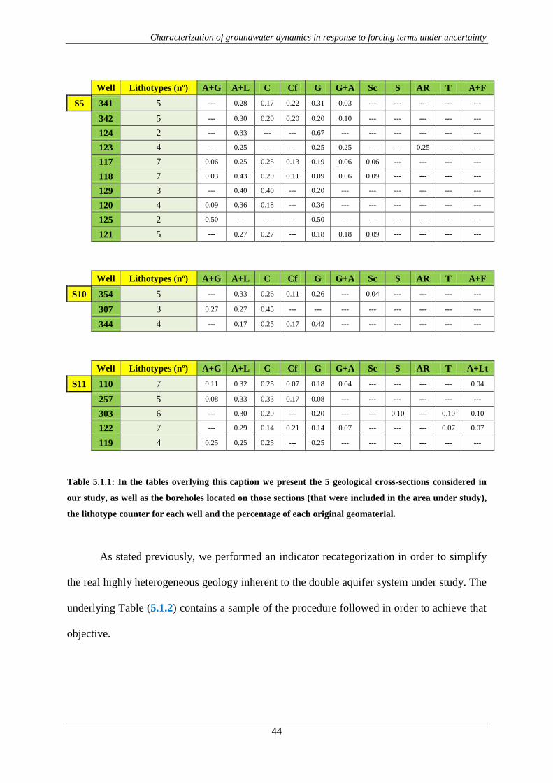
Characterization of groundwater dynamics in response to forcing terms under uncertainty
44
Well Lithotypes (nº) A+G A+L C Cf G G+A Sc S AR T A+F
S5 341 5 --- 0.28 0.17 0.22 0.31 0.03 --- --- --- --- ---
342 5 --- 0.30 0.20 0.20 0.20 0.10 --- --- --- --- ---
124 2 --- 0.33 --- --- 0.67 --- --- --- --- --- ---
123 4 --- 0.25 --- --- 0.25 0.25 --- --- 0.25 --- ---
117 7 0.06 0.25 0.25 0.13 0.19 0.06 0.06 --- --- --- ---
118 7 0.03 0.43 0.20 0.11 0.09 0.06 0.09 --- --- --- ---
129 3 --- 0.40 0.40 --- 0.20 --- --- --- --- --- ---
120 4 0.09 0.36 0.18 --- 0.36 --- --- --- --- --- ---
125 2 0.50 --- --- --- 0.50 --- --- --- --- --- ---
121 5 --- 0.27 0.27 --- 0.18 0.18 0.09 --- --- --- ---
Well Lithotypes (nº) A+G A+L C Cf G G+A Sc S AR T A+F
S10 354 5 --- 0.33 0.26 0.11 0.26 --- 0.04 --- --- --- ---
307 3 0.27 0.27 0.45 --- --- --- --- --- --- --- ---
344 4 --- 0.17 0.25 0.17 0.42 --- --- --- --- --- ---
Well Lithotypes (nº) A+G A+L C Cf G G+A Sc S AR T A+Lt
S11 110 7 0.11 0.32 0.25 0.07 0.18 0.04 --- --- --- --- 0.04
257 5 0.08 0.33 0.33 0.17 0.08 --- --- --- --- --- ---
303 6 --- 0.30 0.20 --- 0.20 --- --- 0.10 --- 0.10 0.10
122 7 --- 0.29 0.14 0.21 0.14 0.07 --- --- --- 0.07 0.07
119 4 0.25 0.25 0.25 --- 0.25 --- --- --- --- --- ---
Table 5.1.1: In the tables overlying this caption we present the 5 geological cross-sections considered in
our study, as well as the boreholes located on those sections (that were included in the area under study),
the lithotype counter for each well and the percentage of each original geomaterial.
As stated previously, we performed an indicator recategorization in order to simplify
the real highly heterogeneous geology inherent to the double aquifer system under study. The
underlying Table (5.1.2) contains a sample of the procedure followed in order to achieve that
objective.

Characterization of groundwater dynamics in response to forcing terms under uncertainty
45
Well Re-classified categories Depth [m]
at 167 (m.a.s.l.) L1 L2 Indicators
349 Argilla e Limo 4.97 A L 1
349 Argilla con Ghiaia 9.54 A G 1
349 Ghiaia 11.68 G --- 3
349 Sabbia Cementata 14.96 S --- 4
349 Conglomerato (Ghiaia Cementata) 23.56 C --- 4
349 Ghiaia 25.12 G --- 3
349 Argilla e Limo 27.17 A L 1
349 Sabbia Cementata 31.16 S --- 4
349 Conglomerato (Ghiaia Cementata) 36.92 C --- 4
349 Argilla e Limo 44.05 A L 1
349 Ghiaia 49.27 G --- 3
349 Argilla e Limo 51.70 A L 1
349 Ghiaia 58.69 G --- 3
349 Argilla e Limo 62.35 A L 1
349 Conglomerato (Ghiaia Cementata) 65.11 C --- 4
349 Ghiaia 66.25 G --- 3
349 Conglomerato (Ghiaia Cementata) 67.34 c fess. --- 5
349 Ghiaia 72.75 G --- 3
349 Argilla e Limo 76.70 A L 1
349 Conglomerato (Ghiaia Cementata) 81.04 C --- 4
Table 5.1.2: We did use the conversion established in Table 4.1.1, to obtain the final indicator values (last
column on the right). Here we also show the main lithologies identified at different depths, from a
reference topographic height of 167 meters above sea level (m.a.s.l.).

Characterization of groundwater dynamics in response to forcing terms under uncertainty
46
5.2. Variogram analysis and indicator variogram model fitting results
A detailed geospatial analysis of the indicator-based variables is performed and three
principal anisotropy directions are identified (North-South, N-S; West-East, W-E; and
vertical). This finding is consistent with field observations and lithological interpretations for
the area where, e.g. the river network (and therefore the depositional trends) is aligned along
the N-S direction. Table 5.2.1 summarizes the parameters of the exponential indicator
variograms which are estimated on the basis of their empirical counterparts and are adopted
for the SISIM simulations. The selection of the exponential model has been based on the least
square criterion and standard analysis of cross-validation errors (details not reported).
Lithology
class Sill
Ranges [m] – SISIM
(N-S / W-E / Vertical)
F1 0.246 1830 / 1280 / 37
F2 0.017 700 / 470 / 20
F3 0.173 1240 / 910 / 34
F4 0.167 860 / 670 / 20
F5 0.098 1220 / 900 / 36
Table 5.2.1: Indicator variogram model parameters estimated for the five hydrofacies and for the SISIM
technique. A zero nugget is estimated for all models.
An exponential model is also selected to characterize the structure of the spatial
dependence of the two underlying Gaussian fields employed in the TPS method. The
parameters of the variograms of these fields are estimated through the iterative procedure
presented by Emery (2007).
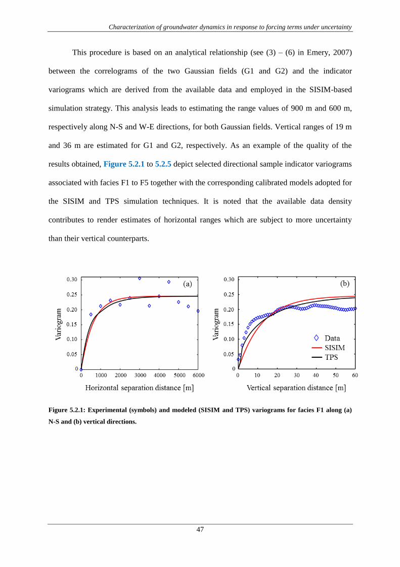
Characterization of groundwater dynamics in response to forcing terms under uncertainty
47
This procedure is based on an analytical relationship (see (3) – (6) in Emery, 2007)
between the correlograms of the two Gaussian fields (G1 and G2) and the indicator
variograms which are derived from the available data and employed in the SISIM-based
simulation strategy. This analysis leads to estimating the range values of 900 m and 600 m,
respectively along N-S and W-E directions, for both Gaussian fields. Vertical ranges of 19 m
and 36 m are estimated for G1 and G2, respectively. As an example of the quality of the
results obtained, Figure 5.2.1 to 5.2.5 depict selected directional sample indicator variograms
associated with facies F1 to F5 together with the corresponding calibrated models adopted for
the SISIM and TPS simulation techniques. It is noted that the available data density
contributes to render estimates of horizontal ranges which are subject to more uncertainty
than their vertical counterparts.
Figure 5.2.1: Experimental (symbols) and modeled (SISIM and TPS) variograms for facies F1 along (a)
N-S and (b) vertical directions.
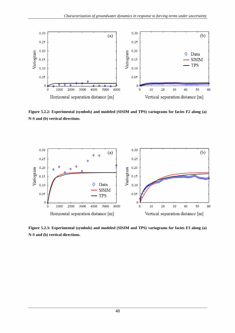
Characterization of groundwater dynamics in response to forcing terms under uncertainty
48
Figure 5.2.2: Experimental (symbols) and modeled (SISIM and TPS) variograms for facies F2 along (a)
N-S and (b) vertical directions.
Figure 5.2.3: Experimental (symbols) and modeled (SISIM and TPS) variograms for facies F3 along (a)
N-S and (b) vertical directions.

Characterization of groundwater dynamics in response to forcing terms under uncertainty
49
Figure 5.2.4: Experimental (symbols) and modeled (SISIM and TPS) variograms for facies F4 along (a)
N-S and (b) vertical directions.
Figure 5.2.5: Experimental (symbols) and modeled (SISIM and TPS) variograms for facies F5 along (a)
N-S and (b) vertical directions.
The shape of the variograms near the origin is linked to the regularity of the
boundaries between mineralogical domains (Emery, 2007). In particular, the exponential
variogram model is smoother than the spherical at the origin and is associated with more
regular boundaries. In contrast, the spherical model increases linearly (close to the origin) and
entails a more erratic boundary between the simulated domains.
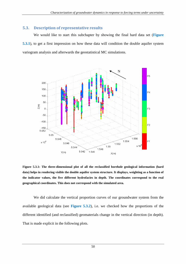
Characterization of groundwater dynamics in response to forcing terms under uncertainty
50
5.3. Description of representative results
We would like to start this subchapter by showing the final hard data set (Figure
5.3.1), to get a first impression on how these data will condition the double aquifer system
variogram analysis and afterwards the geostatistical MC simulations.
Figure 5.3.1: The three-dimensional plot of all the reclassified borehole geological information (hard
data) helps in rendering visible the double aquifer system structure. It displays, weighting as a function of
the indicator values, the five different hydrofacies in depth. The coordinates correspond to the real
geographical coordinates. This does not correspond with the simulated area.
We did calculate the vertical proportion curves of our groundwater system from the
available geological data (see Figure 5.3.2), i.e. we checked how the proportions of the
different identified (and reclassified) geomaterials change in the vertical direction (in depth).
That is made explicit in the following plots.
N

Characterization of groundwater dynamics in response to forcing terms under uncertainty
51
Figure 5.3.2: The left plot displays the raw proportion curves calculated in depth whereas the right plot
shows the smoother proportion curves along the vertical direction (smoothing factor = 2). Elevation is
expressed in meters. These proportions are assumed to be stationary across the full area under study,
including the final smaller simulated domain.
The hard data coordinates, the corresponding indicator values, the bench height and
the smoothing factor were used as input. The bench height corresponds to the actual vertical
discretization length in order to calculate the vertical proportions. The smoothing factor is a
set value (input) that allows calculating a moving average over the benches located above and
below the bench under consideration.
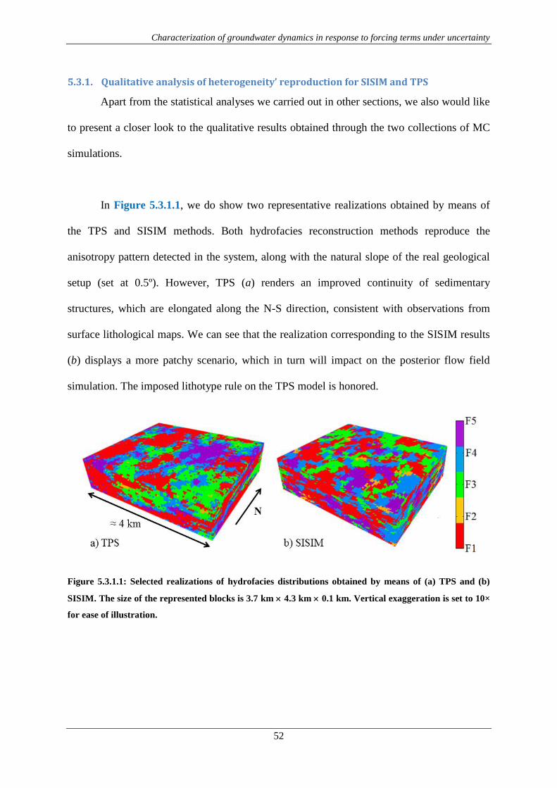
Characterization of groundwater dynamics in response to forcing terms under uncertainty
52
5.3.1. Qualitative analysis of heterogeneity’ reproduction for SISIM and TPS
Apart from the statistical analyses we carried out in other sections, we also would like
to present a closer look to the qualitative results obtained through the two collections of MC
simulations.
In Figure 5.3.1.1, we do show two representative realizations obtained by means of
the TPS and SISIM methods. Both hydrofacies reconstruction methods reproduce the
anisotropy pattern detected in the system, along with the natural slope of the real geological
setup (set at 0.5º). However, TPS (a) renders an improved continuity of sedimentary
structures, which are elongated along the N-S direction, consistent with observations from
surface lithological maps. We can see that the realization corresponding to the SISIM results
(b) displays a more patchy scenario, which in turn will impact on the posterior flow field
simulation. The imposed lithotype rule on the TPS model is honored.
Figure 5.3.1.1: Selected realizations of hydrofacies distributions obtained by means of (a) TPS and (b)
SISIM. The size of the represented blocks is 3.7 km 4.3 km 0.1 km. Vertical exaggeration is set to 10×
for ease of illustration.

Characterization of groundwater dynamics in response to forcing terms under uncertainty
53
5.3.2. Statistical analysis of SISIM and TPS output volumetric proportions
This subchapter is devoted to illustrate some of the statistical results obtained from the
analysis of the raw geostatiscal simulations, corresponding to the two employed
methodologies.
We firstly studied the range/spread of values, realization per realization, and for each
hydrofacies. The wider range of output values that TPS introduced, which will impact on the
following stages of this work, is possible to be identified in Figure 5.3.2.1. However, SISIM
shows more compact behavior around its input volumetric proportion although its distribution
of possible outcomes is not centered at that value. Contrarily, TPS results do show a bigger
spread, but centered on the input volumetric proportion value.
Figure 5.3.2.1: On the X axis we plot the (%) obtained for each realization (series of colored dots), as a
function of each indicator class (Y axis). We plot the results corresponding to the SISIM (a) and the TPS
(b) methods. Star symbols mark the expected input volumetric proportion, imposed by the real geological
database.
a) b)
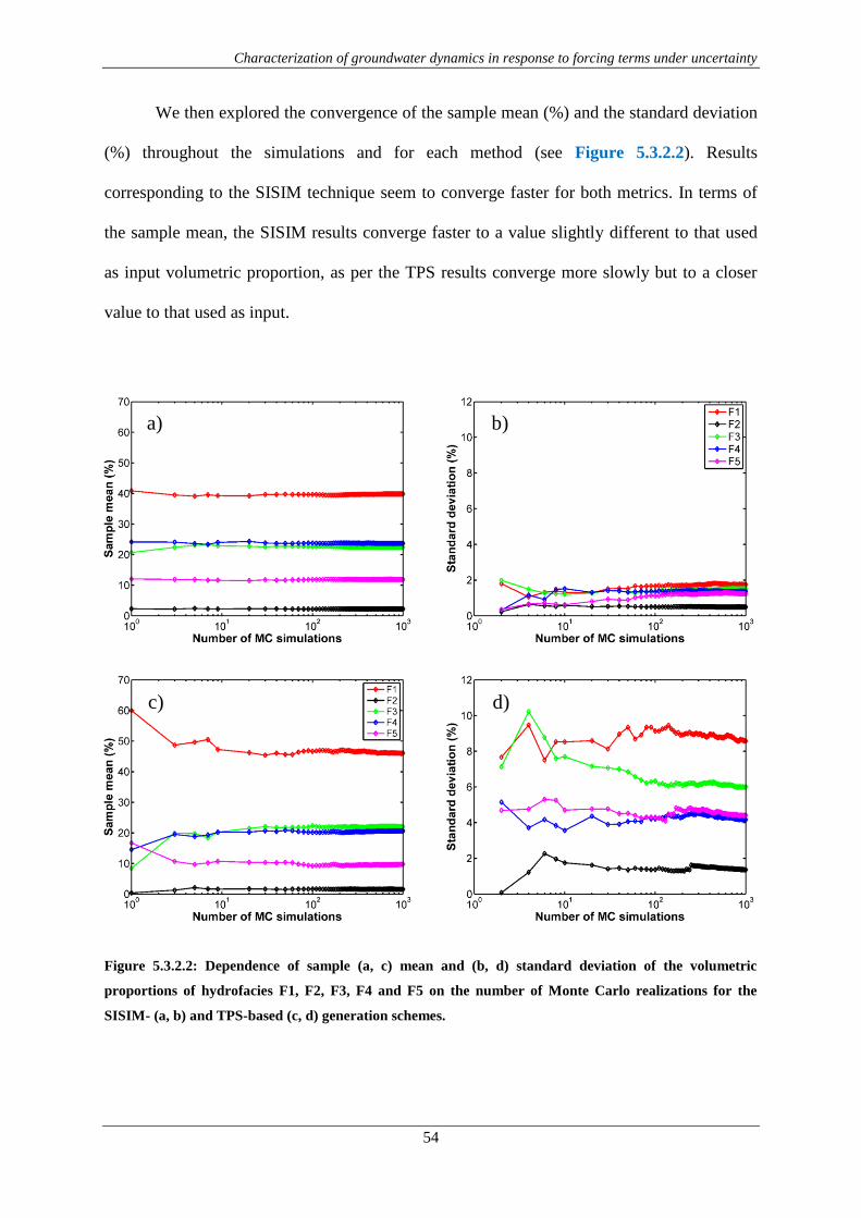
Characterization of groundwater dynamics in response to forcing terms under uncertainty
54
We then explored the convergence of the sample mean (%) and the standard deviation
(%) throughout the simulations and for each method (see Figure 5.3.2.2). Results
corresponding to the SISIM technique seem to converge faster for both metrics. In terms of
the sample mean, the SISIM results converge faster to a value slightly different to that used
as input volumetric proportion, as per the TPS results converge more slowly but to a closer
value to that used as input.
Figure 5.3.2.2: Dependence of sample (a, c) mean and (b, d) standard deviation of the volumetric
proportions of hydrofacies F1, F2, F3, F4 and F5 on the number of Monte Carlo realizations for the
SISIM- (a, b) and TPS-based (c, d) generation schemes.
a) b)
c) d)

Characterization of groundwater dynamics in response to forcing terms under uncertainty
55
We plot the following Figures (5.3.2.3 and 5.3.2.4) in order to better visualize and
further understand the spread of volumetric proportions (%) throughout the simulation
process. The bin classes used to build up the histograms have been calculated as follows: the
minimum and maximum values for each hydrofacies histogram correspond to those imposed
by the set composed of the 1000 simulations, for both SISIM and TPS. Then, each bin differs
from the next in one full point of (%).
Figure 5.3.2.3: Histograms depicting the volumetric proportions obtained from the full set of 1000 SISIM
simulations. The vertical lines do show the position of the input volumetric proportion calculated from
the geological database.
The histograms show typical Gaussian distributions of the output volumetric
proportion (%) values although SISIM fails to reproduce (in the mean) the input volumetric
proportions for 3 of the hydrofacies. The less abundant lithotype (F2) seems to be the best
reproduced.

Characterization of groundwater dynamics in response to forcing terms under uncertainty
56
Figure 5.3.2.4: Histograms depicting the volumetric proportions obtained from the full set of 1000 TPS
simulations. The vertical lines do show the position of the input volumetric proportion calculated from
the geological database.
The histograms show typical Gaussian distributions of the output volumetric
proportion (%) values, rather flat compared to the SISIM counterparts. That higher variability
of the output has a direct impact on the flow field simulations and the resulting hydraulic
head distributions (which will be analyzed later on).
TPS results, conversely to SISIM, reproduce (in the mean) quite accurately the input
volumetric proportions for 4 of the hydrofacies. Only F5, the fractured conglomerates
(second less abundant indicator after F2, the sands), show a slightly skewed behavior towards
the left in the (%) distribution.

Characterization of groundwater dynamics in response to forcing terms under uncertainty
57
We found that introducing a tolerance respect the original input volumetric
proportions, we could gain information respect its over and underestimation as a function of
the generation scheme (Figure 5.3.2.5). We set a tolerance of ±10% for the most abundant
hydrofacies F1, followed by a ±5% for F3 and F4, whereas a ±2.5% and a ±0.5% were set for
F5 and F2 respectively.
Figure 5.3.2.5: Charts showing the amount of MC simulations that whether over (a, c) and/or
underestimated (b, d) the input volumetric proportions, for both SISIM (a, b) and TPS (c, d).
SISIM tends to overestimate the input volumetric proportions when the indicator is
less abundant, but almost no underestimation (for those tolerances) is found in our results. On
the other hand, TPS tends to overestimate evenly throughout the different indicator classes
while tends to underestimate more the input volumetric proportions of those less abundant
simulated geomaterials (i.e. F2 and F5).
a) b)
c) d)

Characterization of groundwater dynamics in response to forcing terms under uncertainty
58
5.3.3. Variogram calculations from output simulations (SISIM and TPS) checking input
parameters honoring
We employed well established software(s) (Deutsch and Journel (1997) for SISIM;
algorithms and codes presented by Xu et al. (2006) and Emery (2007) for TPS). We
performed tests on the ability of those codes to properly generate multiple system
realizations. Table 5.3.3.1 lists the material volumetric proportions inferred from the
available data and employed in the simulation process together with the sample average and
standard deviation of the volumetric proportions calculated for each facies and for both
simulation methods.
Hydrofacies Input hydrofacies
proportions SISIM SISIM TPS TPS
F1 43.6% 39.8% 1.7% 46.1% 8.6%
F2 1.8% 2.2% 0.5% 1.6% 1.4%
F3 22.3% 22.4% 1.5% 22.0% 6.0%
F4 21.2% 23.7% 1.4% 20.6% 4.3%
F5 11.1% 11.9% 1.2% 9.7% 4.4%
Table 5.3.3.1: Input and simulated volumetric proportions for the five hydrofacies. Average (i; i =
SISIM, TPS) and standard deviation (i) of the volumetric proportions are calculated for each facies on
the basis of N = 1000 realizations.
On these bases, we judge our results to be of acceptable quality. A corresponding
check has been performed on the variogram along the vertical direction calculated from
selected realizations.
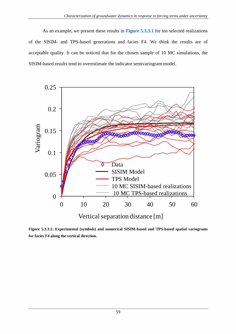
Characterization of groundwater dynamics in response to forcing terms under uncertainty
59
As an example, we present these results in Figure 5.3.3.1 for ten selected realizations
of the SISIM- and TPS-based generations and facies F4. We think the results are of
acceptable quality. It can be noticed that for the chosen sample of 10 MC simulations, the
SISIM-based results tend to overestimate the indicator semivariogram model.
Figure 5.3.3.1: Experimental (symbols) and numerical SISIM-based and TPS-based spatial variograms
for facies F4 along the vertical direction.
0
0.05
0.1
0.15
0.2
0.25
0 10 20 30 40 50 60
Var
iog
ram
Vertical separation distance [m]
Data
SISIM Model
TPS Model
10 MC SISIM-based realizations
10 MC TPS-based realizations

Characterization of groundwater dynamics in response to forcing terms under uncertainty
60
5.3.4. Sample LogK fields for mean (µ) and variance (σ2), from SISIM and TPS
Finally, we present in this subchapter a collection of results regarding the sample
mean and variance of the LogK fields obtained from the performed geostatistical simulations.
As mentioned in previous chapters, we imposed for each simulated indicator class a constant
K value.
We wanted to study the impact of the reconstruction method, including the effect of
the conditioning data, on the average LogK field. What the following plots tell us is valuable
information to better understand the results of the flow field simulations (see Figures 5.3.4.1
and 5.3.4.2).
These plots show vertical cross-sections along the N-S and the W-E directions, with
the sample mean and variance of the corresponding LogK fields obtained from the 1000
realizations and acquired with each simulation method. The vertical scale has been
exaggerated 25 times in order to improve the visualization of the outcome, though distortion
of the geological structures is introduced (unavoidable). It is important to remark at this point,
that any of these vertical cross-sections intersects any actual conditioning borehole data.
Regarding the SISIM results, we can see that persistent clusters of the equivalent to
fine materials (F1) are found at the northern and southern subdomains. That suggests that we
are close to some of the actual conditioning boreholes and that SISIM embeds this influence
in its final outcome.
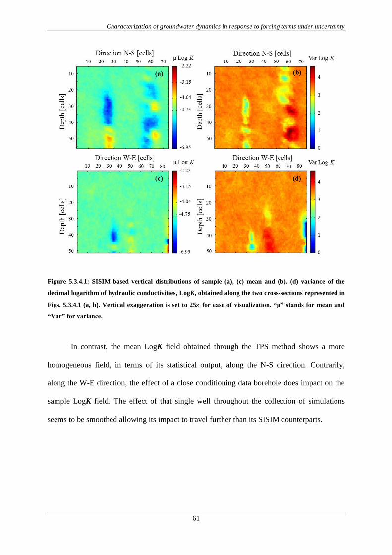
Characterization of groundwater dynamics in response to forcing terms under uncertainty
61
Figure 5.3.4.1: SISIM-based vertical distributions of sample (a), (c) mean and (b), (d) variance of the
decimal logarithm of hydraulic conductivities, LogK, obtained along the two cross-sections represented in
Figs. 5.3.4.1 (a, b). Vertical exaggeration is set to 25 for ease of visualization. “μ” stands for mean and
“Var” for variance.
In contrast, the mean LogK field obtained through the TPS method shows a more
homogeneous field, in terms of its statistical output, along the N-S direction. Contrarily,
along the W-E direction, the effect of a close conditioning data borehole does impact on the
sample LogK field. The effect of that single well throughout the collection of simulations
seems to be smoothed allowing its impact to travel further than its SISIM counterparts.
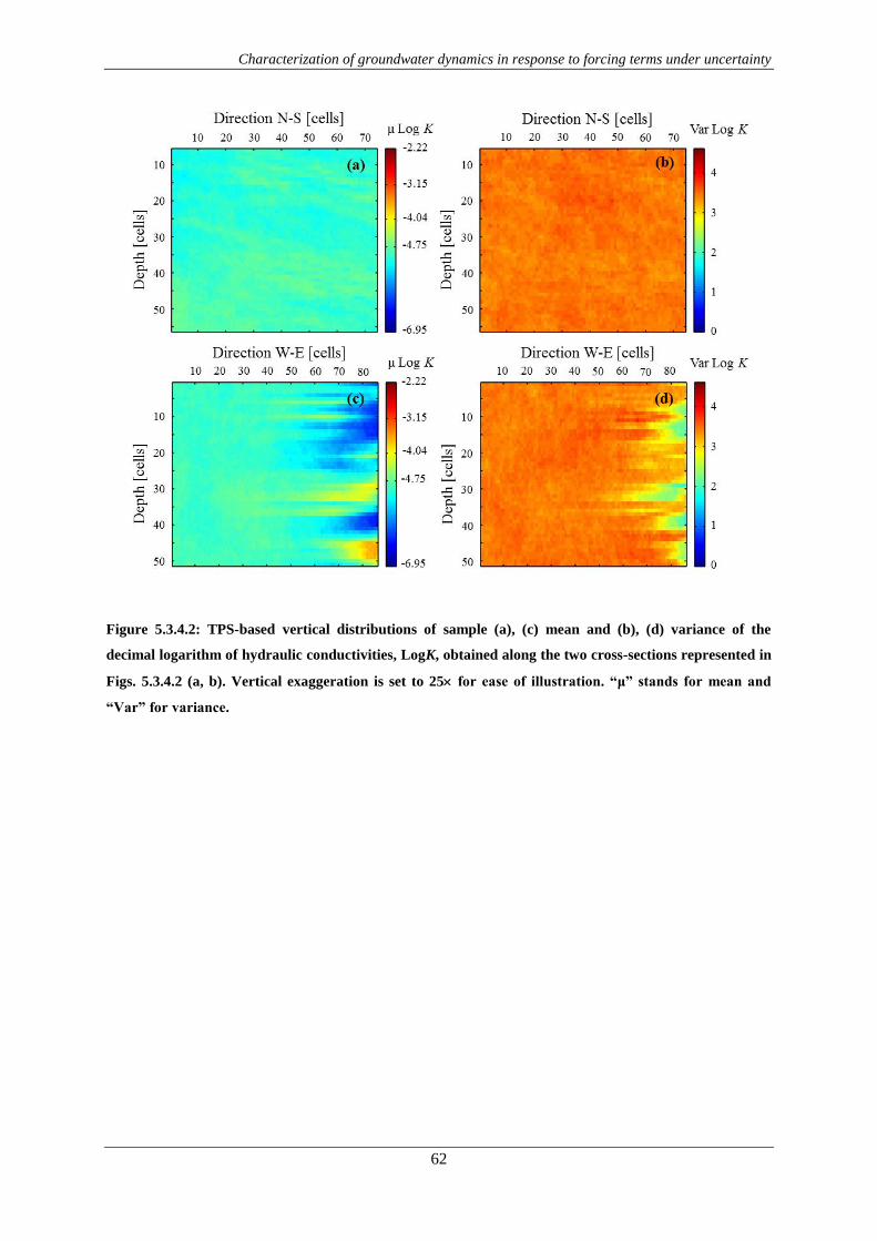
Characterization of groundwater dynamics in response to forcing terms under uncertainty
62
Figure 5.3.4.2: TPS-based vertical distributions of sample (a), (c) mean and (b), (d) variance of the
decimal logarithm of hydraulic conductivities, LogK, obtained along the two cross-sections represented in
Figs. 5.3.4.2 (a, b). Vertical exaggeration is set to 25 for ease of illustration. “μ” stands for mean and
“Var” for variance.

Characterization of groundwater dynamics in response to forcing terms under uncertainty
63
6. Flow field simulations
In this chapter we describe the most relevant results regarding the flow simulations
performed by means of MODFLOW, over the two sets of 1000 of geostatistical MC
realizations obtained with SISIM and TPS schemes.
6.1. Stating the problem: modeling details and procedure
The generated sample of stochastic realizations of (conditional) three-dimensional
hydrofacies distributions are employed to simulate a steady-state convergent flow scenario
due to pumping. The flow problem is solved through the code MODFLOW (McDonald et al.,
1988). Noting that at the large field scale of investigation the spatial arrangement of
lithotypes is a key driver for the distribution of groundwater flow quantities, we adopt here a
composite medium approach (Winter et. al., 2003) where the spatial location of facies is
uncertain and their hydraulic attributes are deterministically known.
In Table 6.1.1 we set the values for hydraulic conductivity KFi associated with facies
Fi (i = 1, ..., 5). These values are inferred from the results of geostatistical inverse modeling
of the large scale groundwater system studied by Bianchi Janetti et al. (2011) and are used
here for consistency. Values have been kept isotropic in the three-dimensional space and do
not vary inside each indicator, i.e. K only changes from Fi to Fj but not in the same
hydrofacies class or indicator.

Characterization of groundwater dynamics in response to forcing terms under uncertainty
64
Kx / Ky / Kz [m/s]
F1 (Fine materials) 1.1210-7
F2 (Sands) 1.7910-5
F3 (Gravels) 7.1610-4
F4 (Conglomerates) 9.0910-5
F5 (Fractured conglomerates) 6.0510-3
Table 6.1.1: Hydraulic conductivity values inferred from the results of the numerical inverse modeling
carried out by Bianchi Janetti et al. (2011). The values have been kept isotropic for the current numerical
study.
Statistical analysis of calculated hydraulic heads is performed in terms of low-order
moments (mean and co-variance) and probability density functions (pdfs) by considering
point and vertically averaged values. The latter are evaluated along segments of thickness B
= 10 m, 20 m and 100 m (i.e., corresponding to 1/10 B, 1/5 B, and B, the complete thickness
of the domain), to simulate completely and partially screened borehole readings.
6.1.1. Numerical grid
The numerical mesh employed for the flow simulations (Figure 6.1.1.1) is built by
further refinement of the hydrofacies generation grid along the horizontal directions, resulting
in a regular horizontal grid spacing of x' = y' = x / 2 = 25 m. The vertical discretization
grid adopted for the flow simulations coincides with the one adopted for the hydrofacies
generation procedure, i.e. z' = z = 2 m. A fully penetrating pumping well is located
approximately at the center of the domain. We enclose Figure 6.1.1.2 to aid in visualization
of the full area under study, the numerically simulated domain and the hard data.
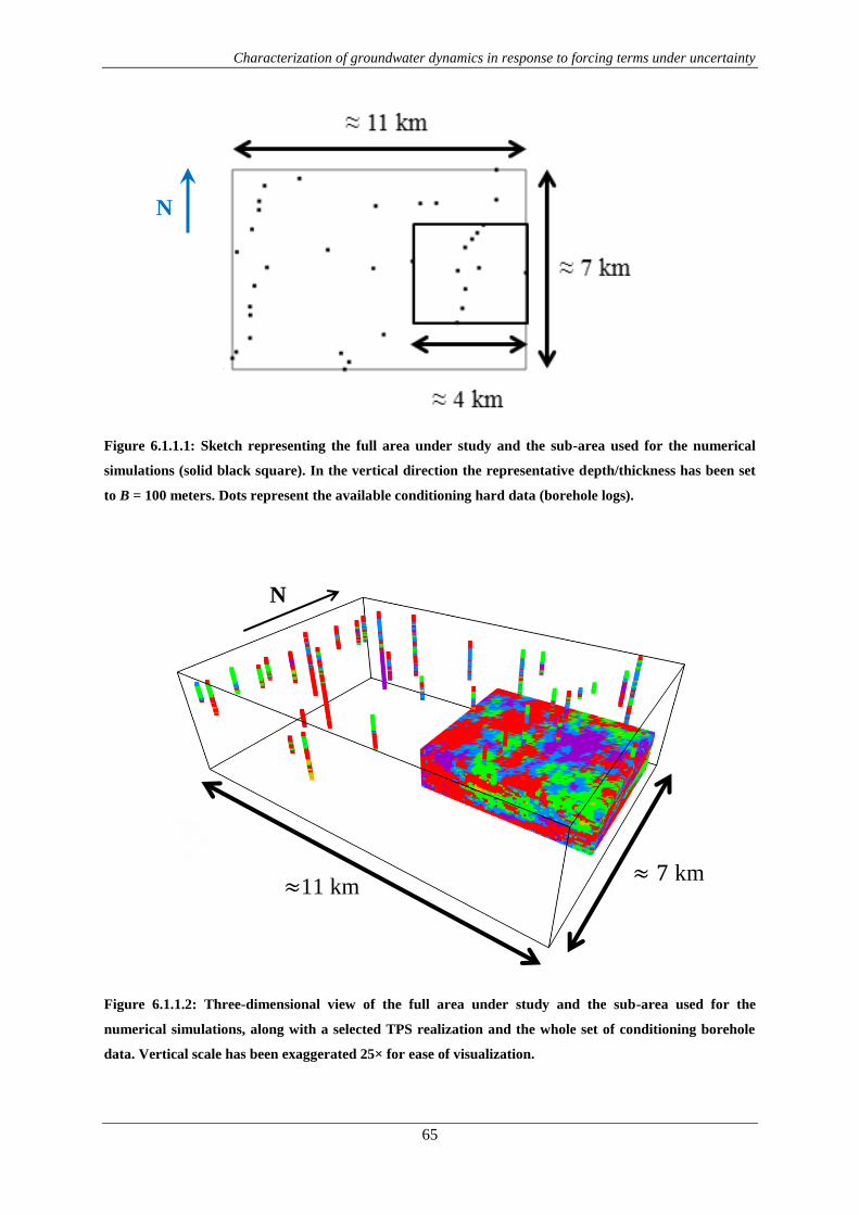
Characterization of groundwater dynamics in response to forcing terms under uncertainty
65
Figure 6.1.1.1: Sketch representing the full area under study and the sub-area used for the numerical
simulations (solid black square). In the vertical direction the representative depth/thickness has been set
to B = 100 meters. Dots represent the available conditioning hard data (borehole logs).
Figure 6.1.1.2: Three-dimensional view of the full area under study and the sub-area used for the
numerical simulations, along with a selected TPS realization and the whole set of conditioning borehole
data. Vertical scale has been exaggerated 25× for ease of visualization.
N
N
11 km km

Characterization of groundwater dynamics in response to forcing terms under uncertainty
66
6.1.2. Boundary conditions
A total pumping rate of 3,000 m3/day is imposed and subdivided among the well
blocks, proportionally to the hydraulic conductivity of each block. Uniform heads of 172.5 m
and 145 m are respectively imposed on the northern and southern edges of the domain to
mimic typical average values of regional hydraulic gradients observed in the area ( 0.7%).
No-flow conditions are imposed along the eastern, western, top and bottom boundaries. The
results of the three-dimensional flow modeling are taken to simulate sets of drawdown
responses monitored at a set of vertical observation boreholes. These enable one to compare
the effect of the stochastic simulation schemes on the response of the system, in terms of
hydraulic head statistics.
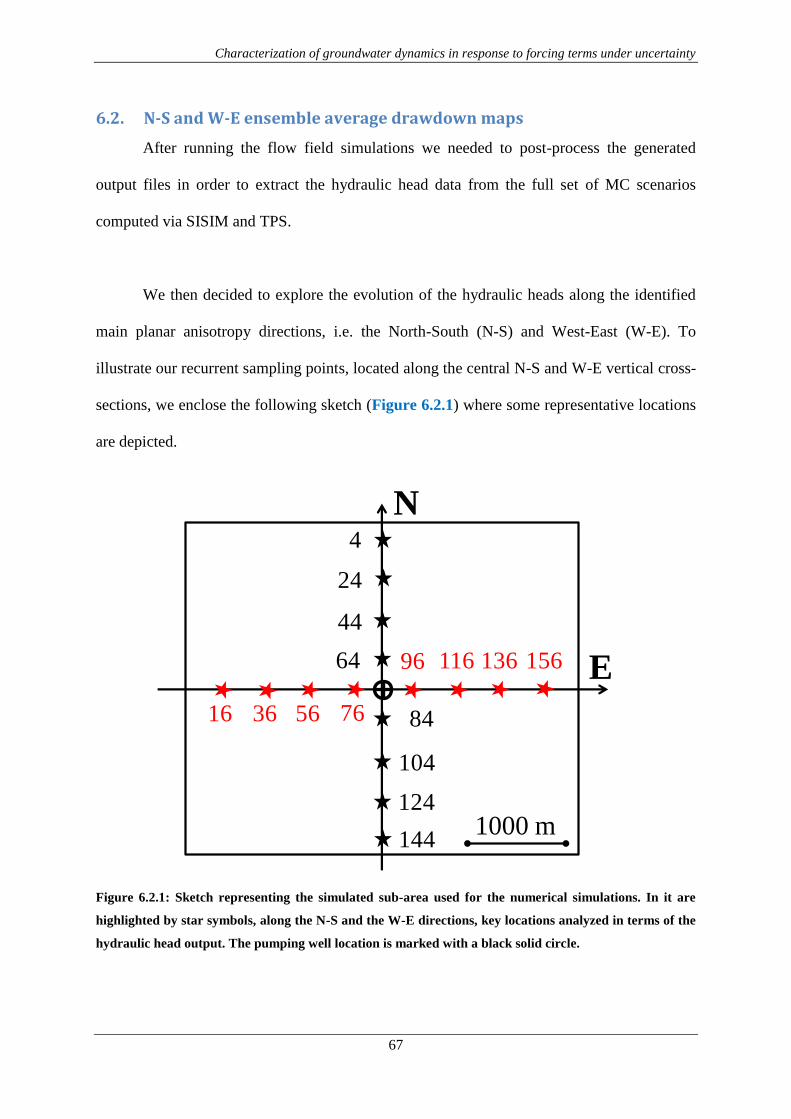
Characterization of groundwater dynamics in response to forcing terms under uncertainty
67
6.2. N-S and W-E ensemble average drawdown maps
After running the flow field simulations we needed to post-process the generated
output files in order to extract the hydraulic head data from the full set of MC scenarios
computed via SISIM and TPS.
We then decided to explore the evolution of the hydraulic heads along the identified
main planar anisotropy directions, i.e. the North-South (N-S) and West-East (W-E). To
illustrate our recurrent sampling points, located along the central N-S and W-E vertical cross-
sections, we enclose the following sketch (Figure 6.2.1) where some representative locations
are depicted.
Figure 6.2.1: Sketch representing the simulated sub-area used for the numerical simulations. In it are
highlighted by star symbols, along the N-S and the W-E directions, key locations analyzed in terms of the
hydraulic head output. The pumping well location is marked with a black solid circle.
64
124
136
76
E
N
1000 m
16 56
4
44
24
144
104
84
156
36
11696
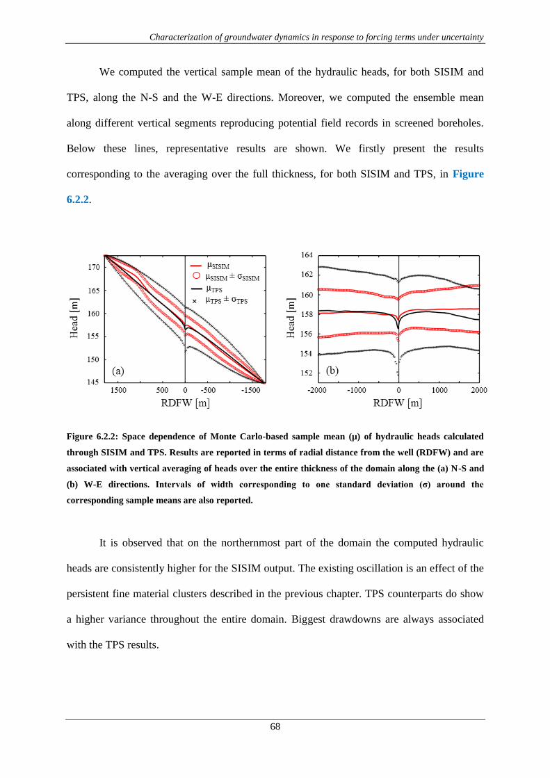
Characterization of groundwater dynamics in response to forcing terms under uncertainty
68
We computed the vertical sample mean of the hydraulic heads, for both SISIM and
TPS, along the N-S and the W-E directions. Moreover, we computed the ensemble mean
along different vertical segments reproducing potential field records in screened boreholes.
Below these lines, representative results are shown. We firstly present the results
corresponding to the averaging over the full thickness, for both SISIM and TPS, in Figure
6.2.2.
Figure 6.2.2: Space dependence of Monte Carlo-based sample mean (µ) of hydraulic heads calculated
through SISIM and TPS. Results are reported in terms of radial distance from the well (RDFW) and are
associated with vertical averaging of heads over the entire thickness of the domain along the (a) N-S and
(b) W-E directions. Intervals of width corresponding to one standard deviation (σ) around the
corresponding sample means are also reported.
It is observed that on the northernmost part of the domain the computed hydraulic
heads are consistently higher for the SISIM output. The existing oscillation is an effect of the
persistent fine material clusters described in the previous chapter. TPS counterparts do show
a higher variance throughout the entire domain. Biggest drawdowns are always associated
with the TPS results.

Characterization of groundwater dynamics in response to forcing terms under uncertainty
69
Figure 6.2.2 illustrates the spatial distribution along selected cross-sections of the
sample mean hydraulic heads calculated for both simulation methods. Results are reported in
terms of radial distance from the well (RDFW; positive for points located North or East of the
pumping well and negative otherwise) and are obtained by vertical averaging point heads
over the complete domain thickness (Figs. 6.2.2.a, b). In Figure 6.2.3 we present the same
results for the upper (Fig. 6.2.3.a, c) and lower (Fig. 6.2.3.b, d) 20 m screened segments.
Intervals of width corresponding to one standard deviation are reported to provide an
indication of the extent of the sample variability induced by the generation method.
Regardless the width of the selected vertical integration segment, it is noted that
hydraulic head values are highest for SISIM in the northern and eastern subregions of the
simulation domain. On the other hand, TPS renders largest average values in the southern and
western parts of the system.
The largest drawdown at the well is always obtained from the TPS method. TPS
yields the largest sample standard deviation of hydraulic heads, consistent with the results
illustrated in Table 5.3.3.1. The observed behavior can be related to the differences in the
internal structure of the hydrofacies and hydraulic conductivity distributions generated with
the two selected methodologies.

Characterization of groundwater dynamics in response to forcing terms under uncertainty
70
Figure 6.2.3: Space dependence of Monte Carlo-based sample mean (µ) of hydraulic heads calculated
through SISIM and TPS. Results are reported in terms of radial distance from the well (RDFW) and are
associated with vertical averaging of heads over the upper 20 m screened segments along the (a) N-S and
(c) W-E directions and with averaging over the lower 20 m screened segments along the (b) N-S and (d)
W-E directions. Intervals of width corresponding to one standard deviation (σ) around the corresponding
sample means are also reported.
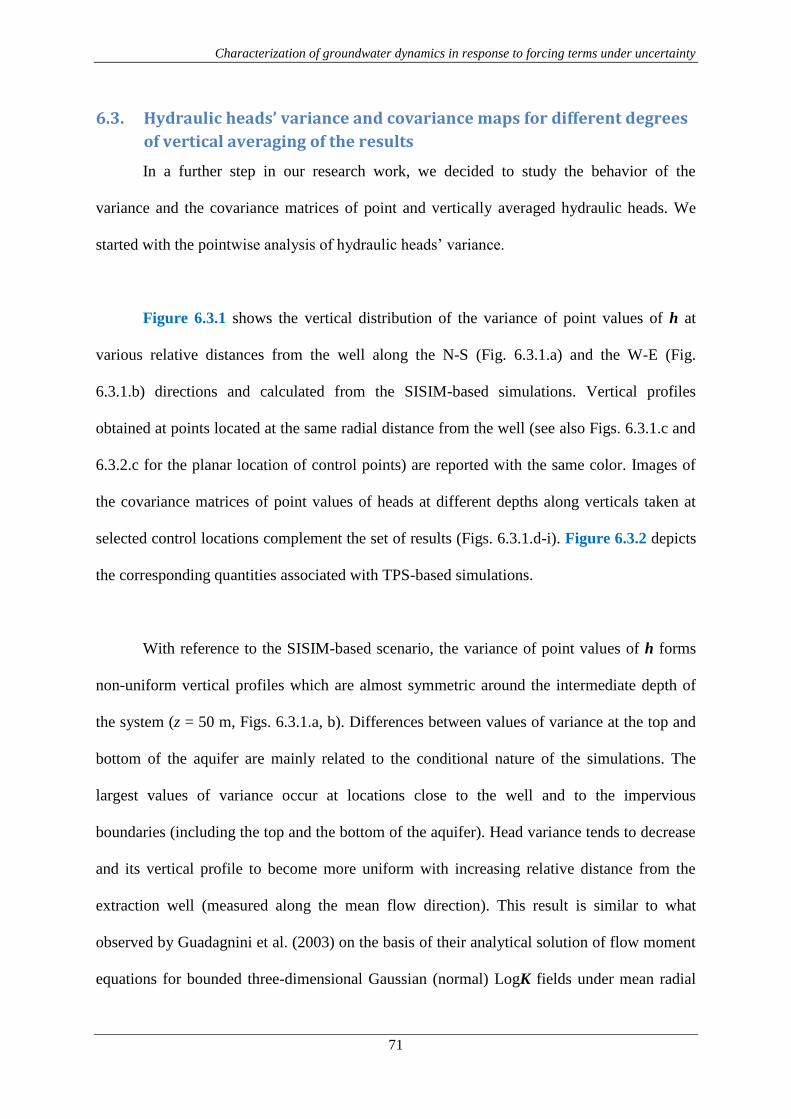
Characterization of groundwater dynamics in response to forcing terms under uncertainty
71
6.3. Hydraulic heads’ variance and covariance maps for different degrees
of vertical averaging of the results
In a further step in our research work, we decided to study the behavior of the
variance and the covariance matrices of point and vertically averaged hydraulic heads. We
started with the pointwise analysis of hydraulic heads’ variance.
Figure 6.3.1 shows the vertical distribution of the variance of point values of h at
various relative distances from the well along the N-S (Fig. 6.3.1.a) and the W-E (Fig.
6.3.1.b) directions and calculated from the SISIM-based simulations. Vertical profiles
obtained at points located at the same radial distance from the well (see also Figs. 6.3.1.c and
6.3.2.c for the planar location of control points) are reported with the same color. Images of
the covariance matrices of point values of heads at different depths along verticals taken at
selected control locations complement the set of results (Figs. 6.3.1.d-i). Figure 6.3.2 depicts
the corresponding quantities associated with TPS-based simulations.
With reference to the SISIM-based scenario, the variance of point values of h forms
non-uniform vertical profiles which are almost symmetric around the intermediate depth of
the system (z = 50 m, Figs. 6.3.1.a, b). Differences between values of variance at the top and
bottom of the aquifer are mainly related to the conditional nature of the simulations. The
largest values of variance occur at locations close to the well and to the impervious
boundaries (including the top and the bottom of the aquifer). Head variance tends to decrease
and its vertical profile to become more uniform with increasing relative distance from the
extraction well (measured along the mean flow direction). This result is similar to what
observed by Guadagnini et al. (2003) on the basis of their analytical solution of flow moment
equations for bounded three-dimensional Gaussian (normal) LogK fields under mean radial
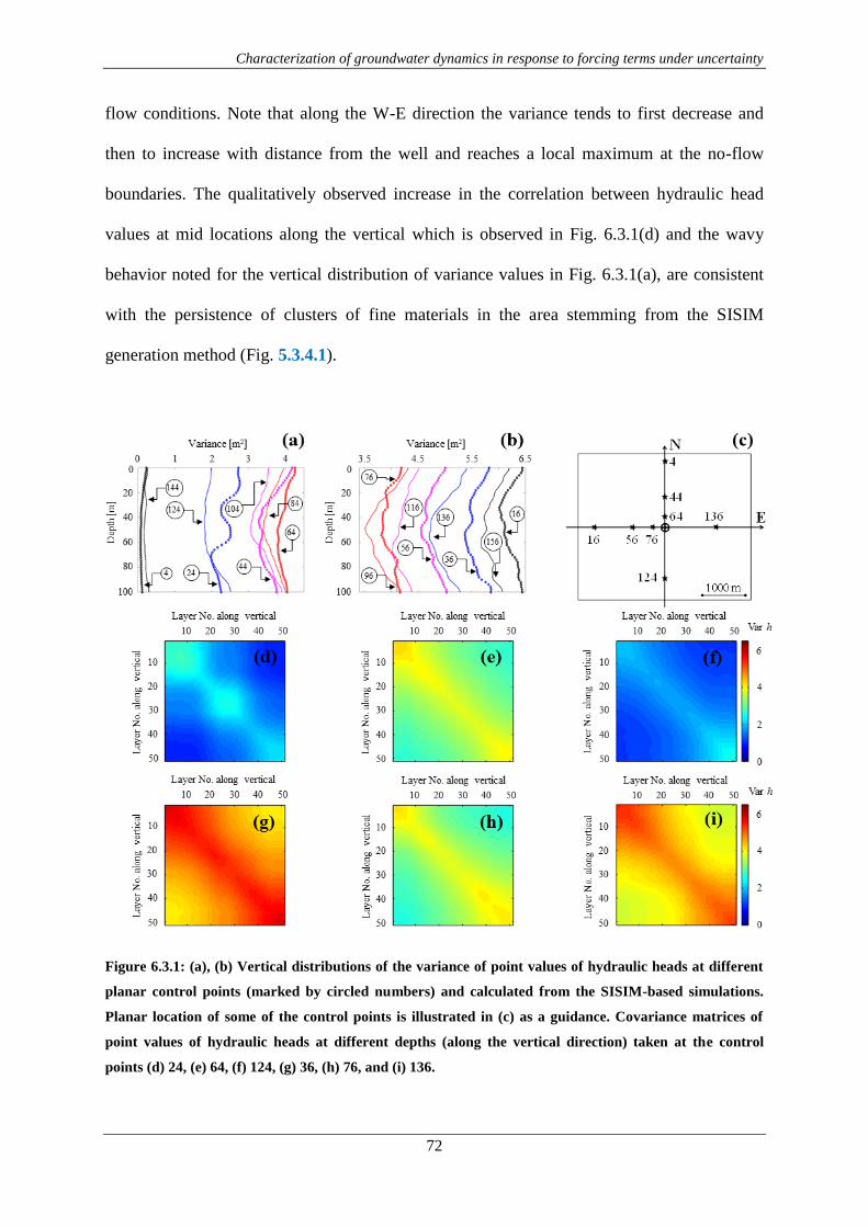
Characterization of groundwater dynamics in response to forcing terms under uncertainty
72
flow conditions. Note that along the W-E direction the variance tends to first decrease and
then to increase with distance from the well and reaches a local maximum at the no-flow
boundaries. The qualitatively observed increase in the correlation between hydraulic head
values at mid locations along the vertical which is observed in Fig. 6.3.1(d) and the wavy
behavior noted for the vertical distribution of variance values in Fig. 6.3.1(a), are consistent
with the persistence of clusters of fine materials in the area stemming from the SISIM
generation method (Fig. 5.3.4.1).
Figure 6.3.1: (a), (b) Vertical distributions of the variance of point values of hydraulic heads at different
planar control points (marked by circled numbers) and calculated from the SISIM-based simulations.
Planar location of some of the control points is illustrated in (c) as a guidance. Covariance matrices of
point values of hydraulic heads at different depths (along the vertical direction) taken at the control
points (d) 24, (e) 64, (f) 124, (g) 36, (h) 76, and (i) 136.

Characterization of groundwater dynamics in response to forcing terms under uncertainty
73
The variance distributions associated with the TPS method are typically characterized
by a reduced vertical variability at locations along the N-S direction (see Fig. 6.3.2.a) and
generally display larger values than those associated with SISIM-based results (compare Figs.
6.3.1.a and 6.3.2.a). Moving along the W-E direction (see Fig. 6.3.2.b), it is noted that the
variance associated with locations at the bottom of the system is consistently larger than that
related to points close to the top. These effects are due to the imposed contact rules between
hydrofacies. These rules tend to reproduce the natural dip of the geological structures in the
system and increase the possibility of occurrence of vertical fluxes.
Figure 6.3.2: (a), (b) Vertical distributions of the variance of point values of hydraulic heads at different
planar control points (marked by circled numbers) and calculated from the TPS-based simulations.
Planar location of some of the control points is illustrated in (c) as a guidance. Covariance matrices of
point values of hydraulic heads at different depths (along the vertical direction) taken at the control
points (d) 24, (e) 64, (f) 124, (g) 36, (h) 76, and (i) 136.

Characterization of groundwater dynamics in response to forcing terms under uncertainty
74
Examples of quantitative results on the effect that vertical averaging of hydraulic
heads along different depth intervals can have on the vertical correlation structure are
reported in Figure 6.3.3. The figure displays SISIM-based covariance matrices of hydraulic
heads at different depths (along verticals) taken at three selected control points along the N-S
and W-E directions and corresponding to two different degrees of refinement of the vertical
averaging thickness, i.e. B = 20 m (Figs. 6.3.3.a-c, g-i) and 10 m (Figs. 6.3.3.d-f, j-l).
Despite the loss of resolution and information along the vertical direction due to spatial
averaging, the main representative features and patterns observed for point values based
covariances (see Figs. 6.3.1.d-f) remain visible. The same observation can be made for TPS-
based simulations, see Figure 6.3.4.
Figure 6.3.3: SISIM-based covariance matrices of hydraulic heads at different depths along verticals
taken at selected control points (a, d) 24, (b, e) 64, (c, f) 124, (g, j) 36, (h, k) 76 and (i, l) 136 (see Figure
6.2.1 for location of control points). Results correspond to two different degrees of refinement of the
vertical averaging thickness, i.e., B = 10 m (Figs. 6.3.3.d-f, j-l) and B = 20 m (Figs. 6.3.3.a-c, g-i).
Horizontal and vertical axes represent the layer numbering associated with each averaging interval.

Characterization of groundwater dynamics in response to forcing terms under uncertainty
75
Figure 6.3.4: TPS-based covariance matrices of hydraulic heads at different depths along verticals taken
at selected control points (a, d) 24, (b, e) 64, (c, f) 124, (g, j) 36, (h, k) 76 and (i, l) 136 (see Figure 6.2.1 for
location of control points). Results correspond to two different degrees of refinement of the vertical
averaging thickness, i.e., B = 10 m (Figs. 6.3.4.d-f, j-l) and B = 20 m (Figs. 6.3.4.a-c, g-i). Horizontal and
vertical axes represent the layer numbering associated with each averaging interval.
Characterization of groundwater dynamics in response to forcing terms under uncertainty
76
6.4. Sample pdf estimation for point and vertically averaged hydraulic
heads
Figure 6.4.1 depicts the N-S and W-E spatial dependence of the sample pdf of
hydraulic heads averaged over the whole aquifer thickness and calculated through the SISIM-
and TPS-based reconstruction methods. The SISIM-based setting appears to be associated
with the largest peakedness of the empirical distributions. Visual inspection of sample pdfs
suggests that a Gaussian model might not always be appropriate to characterize the observed
behavior. These pdfs are sometimes characterized by heavy tails, for which, e.g. an -stable
distribution might be an appropriate interpretive model. On this basis, hydraulic head values
calculated at different locations in the system and averaged along vertical segments of
various thicknesses are examined by (a) assuming that they derive from an -stable
distribution, (b) estimating the parameters of these distributions and (c) analyzing the degree
to which the calibrated distributions fit the numerical results.
Figure 6.4.1: Spatial distribution of the sample pdf of vertically integrated hydraulic heads calculated
through the (a), (c) SISIM- and (b), (d) TPS-based reconstruction methods along the N-S and W-E
directions. RDFW stands for Relative Distance From Well (in meters). White stars mark the location of
the pumping well.

Characterization of groundwater dynamics in response to forcing terms under uncertainty
77
In Figure 6.4.2 we report the results obtained for the top 20 meters averaged vertical
segment, both for SISIM and TPS methods. Qualitatively we observe that the shapes of the
pdfs does not change substantially, remaining more or less Gaussian along the W-E direction
and close to the pumping well, while close to the imposed head boundary conditions the
peakedness of the hydraulic head distributions increases towards its limit value.
Figure 6.4.2: Spatial distribution of the sample pdf of vertically integrated hydraulic heads over the top
20 meters and calculated through the (a), (c) SISIM- and (b), (d) TPS-based reconstruction methods
along the N-S and W-E directions. RDFW stands for Relative Distance From Well (in meters). White
stars mark the location of the pumping well.
A statistical analysis is performed at selected locations, to test the influence of the
averaging procedure along the vertical direction on the simulation results. As an example,
Figure 6.4.3 illustrates the variability along the vertical of SISIM-based hydraulic head
sample pdfs calculated on the basis of the MC simulations at control point 24 (located in the
northern part of the domain, at about 600 m from the prescribed hydraulic head boundary and
1250 m from the well) and for the different averaging intervals considered, i.e. point values
(Fig. 6.4.3.a), B = 10 m (Fig. 6.4.3.b) and B = 20 m (Fig. 6.4.3.c).

Characterization of groundwater dynamics in response to forcing terms under uncertainty
78
The influence of the northern (prescribed head) boundary condition is notable on the
skewness and on the (left) heavy tail of the distributions. The pointwise and vertically
averaged values of h share some notable statistical properties. All sample distributions appear
to be reasonably fitted by an -stable model which is negatively skewed (i.e., 1.0) and
with values ranging between 1.6 and 1.8. The same analysis performed at points lying in
the southern part of the system provides qualitatively similar results, with sample pdfs being
fitted by positively skewed ( 1.0) -stable distributions.
Figure 6.4.3: Vertical distribution of SISIM-based hydraulic head sample pdfs calculated at control point
24 (see Figure 6.2.1) and for the different averaging intervals considered, i.e. (a) point hydraulic head
values, and head values vertically averaged along coordinate z with (b) B = 10 m and (c) B = 20 m.
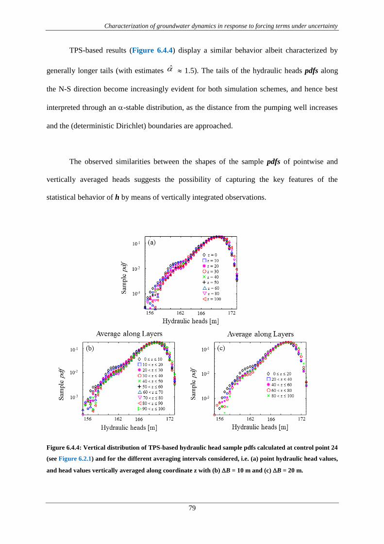
Characterization of groundwater dynamics in response to forcing terms under uncertainty
79
TPS-based results (Figure 6.4.4) display a similar behavior albeit characterized by
generally longer tails (with estimates 1.5). The tails of the hydraulic heads pdfs along
the N-S direction become increasingly evident for both simulation schemes, and hence best
interpreted through an -stable distribution, as the distance from the pumping well increases
and the (deterministic Dirichlet) boundaries are approached.
The observed similarities between the shapes of the sample pdfs of pointwise and
vertically averaged heads suggests the possibility of capturing the key features of the
statistical behavior of h by means of vertically integrated observations.
Figure 6.4.4: Vertical distribution of TPS-based hydraulic head sample pdfs calculated at control point 24
(see Figure 6.2.1) and for the different averaging intervals considered, i.e. (a) point hydraulic head values,
and head values vertically averaged along coordinate z with (b) B = 10 m and (c) B = 20 m.
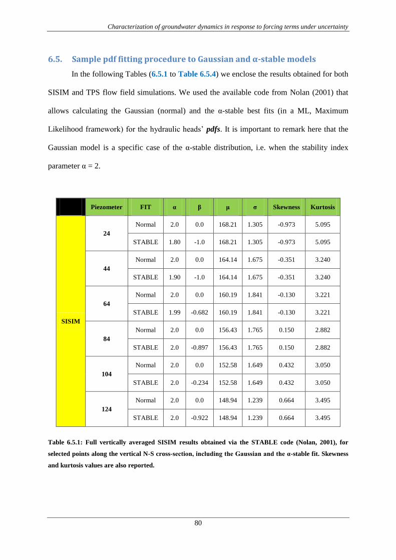
Characterization of groundwater dynamics in response to forcing terms under uncertainty
80
6.5. Sample pdf fitting procedure to Gaussian and α-stable models
In the following Tables (6.5.1 to Table 6.5.4) we enclose the results obtained for both
SISIM and TPS flow field simulations. We used the available code from Nolan (2001) that
allows calculating the Gaussian (normal) and the α-stable best fits (in a ML, Maximum
Likelihood framework) for the hydraulic heads’ pdfs. It is important to remark here that the
Gaussian model is a specific case of the α-stable distribution, i.e. when the stability index
parameter α = 2.
Piezometer FIT α β μ σ
Skewness Kurtosis
SISIM
24
Normal 2.0 0.0 168.21 1.305 -0.973 5.095
STABLE 1.80 -1.0 168.21 1.305 -0.973 5.095
44
Normal 2.0 0.0 164.14 1.675 -0.351 3.240
STABLE 1.90 -1.0 164.14 1.675 -0.351 3.240
64
Normal 2.0 0.0 160.19 1.841 -0.130 3.221
STABLE 1.99 -0.682 160.19 1.841 -0.130 3.221
84
Normal 2.0 0.0 156.43 1.765 0.150 2.882
STABLE 2.0 -0.897 156.43 1.765 0.150 2.882
104
Normal 2.0 0.0 152.58 1.649 0.432 3.050
STABLE 2.0 -0.234 152.58 1.649 0.432 3.050
124
Normal 2.0 0.0 148.94 1.239 0.664 3.495
STABLE 2.0 -0.922 148.94 1.239 0.664 3.495
Table 6.5.1: Full vertically averaged SISIM results obtained via the STABLE code (Nolan, 2001), for
selected points along the vertical N-S cross-section, including the Gaussian and the α-stable fit. Skewness
and kurtosis values are also reported.
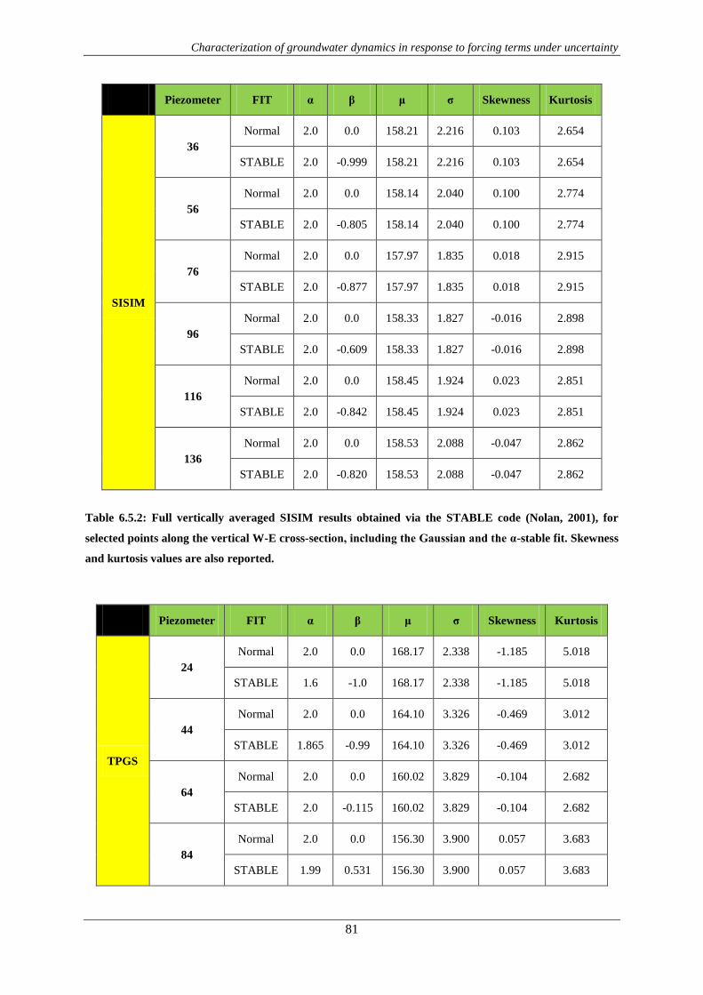
Characterization of groundwater dynamics in response to forcing terms under uncertainty
81
Piezometer FIT α β μ σ
Skewness Kurtosis
SISIM
36
Normal 2.0 0.0 158.21 2.216 0.103 2.654
STABLE 2.0 -0.999 158.21 2.216 0.103 2.654
56
Normal 2.0 0.0 158.14 2.040 0.100 2.774
STABLE 2.0 -0.805 158.14 2.040 0.100 2.774
76
Normal 2.0 0.0 157.97 1.835 0.018 2.915
STABLE 2.0 -0.877 157.97 1.835 0.018 2.915
96
Normal 2.0 0.0 158.33 1.827 -0.016 2.898
STABLE 2.0 -0.609 158.33 1.827 -0.016 2.898
116
Normal 2.0 0.0 158.45 1.924 0.023 2.851
STABLE 2.0 -0.842 158.45 1.924 0.023 2.851
136
Normal 2.0 0.0 158.53 2.088 -0.047 2.862
STABLE 2.0 -0.820 158.53 2.088 -0.047 2.862
Table 6.5.2: Full vertically averaged SISIM results obtained via the STABLE code (Nolan, 2001), for
selected points along the vertical W-E cross-section, including the Gaussian and the α-stable fit. Skewness
and kurtosis values are also reported.
Piezometer FIT α β μ σ
Skewness Kurtosis
TPGS
24
Normal 2.0 0.0 168.17 2.338 -1.185 5.018
STABLE 1.6 -1.0 168.17 2.338 -1.185 5.018
44
Normal 2.0 0.0 164.10 3.326 -0.469 3.012
STABLE 1.865 -0.99 164.10 3.326 -0.469 3.012
64
Normal 2.0 0.0 160.02 3.829 -0.104 2.682
STABLE 2.0 -0.115 160.02 3.829 -0.104 2.682
84
Normal 2.0 0.0 156.30 3.900 0.057 3.683
STABLE 1.99 0.531 156.30 3.900 0.057 3.683

Characterization of groundwater dynamics in response to forcing terms under uncertainty
82
104
Normal 2.0 0.0 152.98 3.405 0.739 3.757
STABLE 1.80 1.0 152.98 3.405 0.739 3.757
124
Normal 2.0 0.0 149.29 2.410 1.496 6.692
STABLE 1.60 1.0 149.29 2.410 1.496 6.692
Table 6.5.3: Full vertically averaged SISIM results obtained via the STABLE code (Nolan, 2001), for
selected points along the vertical N-S cross-section, including the Gaussian and the α-stable fit. Skewness
and kurtosis values are also reported.
Piezometer FIT α β μ σ
Skewness Kurtosis
TPGS
36
Normal 2.0 0.0 158.31 4.131 0.140 2.635
STABLE 2.0 -0.001 158.31 4.131 0.140 2.635
56
Normal 2.0 0.0 158.29 3.947 0.126 2.625
STABLE 2.0 0.0 158.29 3.947 0.126 2.625
76
Normal 2.0 0.0 158.00 3.839 0.067 2.590
STABLE 2.0 -0.010 158.00 3.839 0.067 2.590
96
Normal 2.0 0.0 158.00 3.818 0.108 2.706
STABLE 2.0 0.690 158.00 3.818 0.108 2.706
116
Normal 2.0 0.0 158.28 3.681 0.131 2.755
STABLE 2.0 0.695 158.28 3.681 0.131 2.755
136
Normal 2.0 0.0 158.15 3.431 0.080 2.745
STABLE 2.0 -0.410 158.15 3.431 0.080 2.745
Table 6.5.4: Full vertically averaged TPS results obtained via the STABLE code (Nolan, 2001), for
selected points along the vertical W-E cross-section, including the Gaussian and the α-stable fit. Skewness
and kurtosis values are also reported.

Characterization of groundwater dynamics in response to forcing terms under uncertainty
83
Figures 6.5.1 and 6.5.2 respectively show the N-S and W-E spatial evolution of the
pdf of hydraulic heads obtained after averaging heads along the whole aquifer thickness
(Figures 6.5.1.a-c) or over the top 25 m segment (Figures 6.5.1.d-f) and on the basis of the
SISIM methodology. Empirical hydraulic head pdfs are interpreted by considering the
Gaussian and the -stable models. Each plot in Figures 6.5.1 and 6.5.2 reports the Monte
Carlo sample distribution and corresponding ML fits for the Gaussian and -stable
distributions. The corresponding results associated with the TPS method are depicted in
Figures 6.5.3 and 6.5.4.
The tails of the hydraulic heads’ pdfs along the N-S direction become increasingly
evident for both simulation schemes, and hence best interpreted through an -stable
distribution, as the distance from the pumping well increases. At locations close to the fixed
head boundaries, the distribution is skewed towards values which are representative of the
inner portion of the domain. This behavior is observed for both types of vertically averaged
information.
Conversely, the pdfs of vertically averaged heads along the W-E direction appear to
be well interpreted by a symmetric distribution such as the Gaussian model, regardless the
thickness of the vertical averaging segment and the generation model adopted. These features
could be related to the prescribed boundary conditions which introduce fewer constraints
(through the Monte Carlo realizations) to the heads computed along the W-E direction.

Characterization of groundwater dynamics in response to forcing terms under uncertainty
84
Figure 6.5.1: SISIM-based pdfs of vertically averaged (over the full thickness of the domain) hydraulic
heads at control points (a) 24, (b) 64, and (c) 124 (see Figure 6.2.1). Corresponding results related to
hydraulic heads vertically averaged along the top 25 meters of the domain are also reported for control
points (d) 24, (e) 64, and (f) 124. ML fits for the Gaussian and -stable distributions are also reported.
Figure 6.5.2: SISIM-based pdfs of vertically averaged (over the full thickness of the domain) hydraulic
heads at control points (a) 36, (b) 76, and (c) 136 (see Figure 6.2.1). Corresponding results related to
hydraulic heads vertically averaged along the top 25 meters of the domain are also reported for control
points (d) 36, (e) 76, and (f) 136. ML fits for the Gaussian and -stable distributions are also reported.

Characterization of groundwater dynamics in response to forcing terms under uncertainty
85
Figure 6.5.3: TPS-based pdfs of vertically averaged (over the full thickness of the domain) hydraulic
heads at control points (a) 24, (b) 64, and (c) 124 (see Figure 6.2.1). Corresponding results related to
hydraulic heads vertically averaged along the top 25 meters of the domain are also reported for control
points (d) 24, (e) 64, and (f) 124. ML fits for the Gaussian and -stable distributions are also reported.
Figure 6.5.4: TPS-based pdfs of vertically averaged (over the full thickness of the domain) hydraulic
heads at control points (a) 36, (b) 76, and (c) 136 (see Figure 6.2.1). Corresponding results related to
hydraulic heads vertically averaged along the top 25 meters of the domain are also reported for control
points (d) 36, (e) 76, and (f) 136. ML fits for the Gaussian and -stable distributions are also reported.
Characterization of groundwater dynamics in response to forcing terms under uncertainty
86
Figure 6.5.5.a reports the N-S spatial dependence of estimates associated with the
sample distributions of vertically averaged (over the complete thickness of the domain)
hydraulic heads for both the SISIM- and TPS-based results. In general, we note that the tails
of the head distributions are longer (i.e., is smaller) for TPS- than for SISIM-based
simulations and decrease as the distance from the prescribed (deterministic) head boundaries
increases. For large distances from these boundaries or close to the pumping well the
distributions tend to become Gaussian (i.e., = 2.0). At locations close to the fixed head
boundaries, the distribution is skewed towards values which are representative of the inner
portion of the domain.
Conversely, the pdfs of vertically averaged heads along the W-E direction appear to
be well interpreted by the Gaussian model (i.e., 2.0), regardless the thickness of the
vertical averaging segment and the generation model adopted. The prescribed flux boundary
conditions introduce less constraints (through the Monte Carlo realizations) to the heads
computed along the W-E direction and the shape of the sample head distributions is not
significantly modified when approaching the boundaries.
Figure 6.5.5.b reports the N-S spatial dependence of estimates obtained for the
distribution of vertically averaged hydraulic heads for both the SISIM- and TPS-based
results. Since the scale parameter is linked to the (ensemble) variability of the variable (in
particular its square value is equal to half the variance when α = 2.0), we observe an increase
of with the distance from the fixed head boundaries. Consistent with the analysis
presented above, is significantly larger for the TPS-based results than for their SISIM
counterparts.

Characterization of groundwater dynamics in response to forcing terms under uncertainty
87
Figure 6.5.5: Estimates of (a) stability index ( ) and (b) scale parameter ( ) of hydraulic heads
integrated along the full aquifer thickness versus RDFW (Relative Distance From Well) along the N-S
direction.
0
0.5
1
1.5
2
2.5
3
3.5
-2000-1000010002000
1
1.2
1.4
1.6
1.8
2
2.2
-2000-1000010002000
RDFW[m]
SISIM
TPS
(a) (b)
RDFW[m]
Characterization of groundwater dynamics in response to forcing terms under uncertainty
88
7. Discussion
In this section we present the discussion of the results of the two previous chapters,
regarding the geostatistical and the flow field simulations. We do this in order to come up
with some conclusions and a better insight of the combined information acquired from the
joint analysis of both methodologies’ output.
7.1. Practical applications
Our results provide a basic component which can be employed to quantify a hydraulic
head threshold that might be dangerous for a given location (for instance, an overabstraction
that leads to a pronounced lowering of piezometric head). Probability distributions of
hydraulic heads calculated through different stochastic reconstruction methodologies, provide
a way of comparing and quantifying the uncertainty stemming from competing conceptual
system models and associated with the estimation of the hydraulic head thresholds that might
endanger the equilibrium of protected natural areas.
7.2. Objective and novelty
We aim at analyzing the way hydraulic heads probability distributions (in terms of
functional form and parameters) are affected by the two reconstruction methods adopted for
the aquifer system, i.e. embedding or not a conceptual model of facies contact. We do so by
considering a convergent flow which, to the best of our knowledge, has not been analyzed in
this context and is of critical importance in environmental applications of the kind described
above.

Characterization of groundwater dynamics in response to forcing terms under uncertainty
89
Low-order (statistical) moments (i.e., mean and variance-covariance) of hydraulic
heads in unbounded and bounded domains under uniform (in the mean flow) conditions have
been investigated, amongst others, by: Dagan (1985), Rubin and Dagan (1988, 1989), Osnes
(1995), Ababou et al. (1989), Dagan (1989), Guadagnini and Neuman (1999a, b). Our intent,
in the bibliographic research, was to provide a review of the works dealing with the analysis
of the probability density of hydraulic heads, with specific reference to the non-uniform (in
the mean) flow configuration we analyzed. There are not too many works dealing with this
specific issue. Indeed, this is a strong point of our study and it confirms the novelty of our
analysis.
The target Environmental Performance Metrics (EPMs) we consider are (a) point and
(b) vertically integrated hydraulic heads. The latter are the quantities which can be typically
observed under field conditions, e.g. through screened boreholes, and for instance can be
linked to water levels in natural springs which are fed by confined aquifers. The joint impact
of heterogeneity model and vertical averaging under the combination of natural and forced
flow regimes has not been addressed previously. We have approached this work by taking the
point of view that the basic question is not which model is best, but how the models compare
and what they tell us jointly about the physical quantities and process of interest, i.e. the
probability distribution of hydraulic heads. This is the most that can be done in the absence of
independent physical data or, possibly, in the presence of a very limited set of observations
on the state variable. Of course, model identification is a very relevant and delicate subject,
but goes beyond the scope of the present study. For a deeper insight to this specific issue we
redirect the reader to the works published by Riva et al. (2010, 2011), Panzeri et al. (2013)
and Bianchi Janetti et al. (2012).

Characterization of groundwater dynamics in response to forcing terms under uncertainty
90
We reiterate that we are interested in the comparison between outcomes associated
with two competing models and we do think this to be a relevant aspect. Thorough
understanding and quantification of the influence of a model on the variability of a system
response can also be considered as a first step in a detailed model identification analysis. We
think that such a comparison is of relevance, especially in the presence of (statistically) non-
stationary hydraulic parameter distributions and non-uniform flow conditions of the kind we
analyze here. The study we perform can be framed in the context of probabilistic risk
assessment (PRA) of hydrogeological scenarios, thus facilitating uncertainty quantification
associated with incomplete knowledge of the geological architecture of the system.
Albeit model calibration studies in the context of a truncated plurigaussian framework
have been presented in the past (e.g., Mariethoz et al., 2009) our objective here is different, as
we pose ourselves the question: "How does the adoption of two simulation strategies
embedding different system conceptualizations impact the statistics of the state variable field
in a representative field scale aquifer model?". The outcome of such a study is potentially
relevant in intrinsic vulnerability studies, where one is interested in quantifying the
probability associated with given hydraulic head values at target locations in the system as a
function of the conceptual uncertainty associated with the geological model. This is more
than a sensitivity study on the effect of facies distribution because it includes the effect of
different modeling choices, based on the expertise of the groundwater flow modeler and field
geologist.
Characterization of groundwater dynamics in response to forcing terms under uncertainty
91
7.3. Indicator simulations
When assessing model reliability against controlled synthetic test cases under
different conditions, studies presented in the literature are mainly based on realistic images
where the level of realism is difficult to quantify, as it can be assessed only in qualitative
way. Therefore, given the purpose of our analysis, we preferred considering an actual set of
lithological information which is associated with an observation window which is
representative of a field scale setting. In our specific case, we think we have at our disposal a
reasonably abundant data set, as compared to typically available information content of this
kind for the investigated scale. We further note that we employed the available data not only
for estimation of volumetric proportions or variogram assessment, but also to analyze the
actual hierarchy of the system architecture in the area and, therefore, for the selection of the
reconstruction methodology. When model performance needs to be assessed, then we agree
that the best option is always to start from hypothetical settings, where a ground truth is
clearly defined.
However, we are not aware of a comparative study of the kind we propose in the
manuscript in presence of a non-uniform flow field. Indeed, this is an environmentally
relevant scenario and we decided to analyze the (random) variability of the response of the
system with two relatively simple and well-known techniques which are commonly
employed for aquifer simulation. As such, we decided to compare the effects of the two
techniques by observing the impact of the system conceptualization, as embedded in the
lithotype rule, when all other inputs are kept constant.

Characterization of groundwater dynamics in response to forcing terms under uncertainty
92
7.3.1. Comparison of SISIM and TPS results
From a qualitative point of view it can be noted that TPS renders an improved
continuity of sedimentary structures, which are elongated along the N-S direction,
consistently with observations from surface lithological maps. Both methods reproduce the
anisotropy pattern detected in the system.
Along the N-S direction the SISIM method yields persistent clusters characterized by
small ( 10-7
m/s) and large ( 10-4
m/s) conductivity values while the TPS-based results are
associated with a relatively uniform ( 10-5
m/s) K distribution and a large LogK variance.
A key difference between the fields of LogK sample variance, obtained with the two
methods, lies in the relatively uniform distribution of persistently large values which is
visible in the TPS results. This is opposed to the outcome of SISIM simulations, which are
associated with a spatially heterogeneous pattern (alternating low and large variance values).
The effect of the conditioning data on the spatial persistence of variance values is different
for the two methodologies, due to the geological constraints imposed in the TPS procedure
through the adopted contact rules. These results are consistent with the spatial pattern which
can be detected for single realizations of hydrofacies distributions.
Both simulation methods are conditional on the same dataset. Both techniques are
variogram-based and are directly comparable. Comments about the merits of the truncated
plurigaussian generation technique as opposed to a sequential indicator simulation are
available in, for instance, Mariethoz et al. (2009) and in the Introduction of this manuscript.
This points out the worth and value of numerical studies of the kind we perform, to
understand the type of variability which is imprinted to the system response (in terms of key

Characterization of groundwater dynamics in response to forcing terms under uncertainty
93
statistics of hydraulic heads) by adopting or neglecting conceptual knowledge about the
geological setup of an aquifer.
7.3.2. Providing guidelines
GEOLOGICAL SETUP AND AQUIFER SIMULATIONS
The thickness of the aquifer system is not constant across the area under study where
the borehole network associated with the lithological data is set. The domain we adopt in our
simulations is extracted from the real aquifer system and its thickness was selected to include
its key features observed in the field. In other words, since one of the objectives of this study
is to analyze the way the vertical variability of hydraulic heads is impacted by facies
distribution, boundary conditions and/or source terms (without considering the effect of the
particular geometry of the bottom of the aquifer), we adopt in the following a constant
thickness B = 100 m which is representative of an average thickness of the system in the area.
We start by noting that we did not have availability of hard hydraulic conductivity
data with a level of discretization which was nearly comparable with that of the lithological
information we employed in our study. There is typically conceptual uncertainty associated
with the selection of a model which can represent the heterogeneity of an aquifer at different
scales of observation. Here, we are interested in an observation window which encompasses
horizontal and vertical scale lengths of the order of 4000 m and 100 m, respectively. At these
scales the distribution of lithotypes in the system is a key driver for the distribution of
groundwater flow quantities. On the other hand, the spatial heterogeneity of hydraulic
parameters within a given lithotype is relevant at smaller scales of observations as seen, for
example, in the works of Winter et al. (2003) and Riva et al. (2006, 2008, 2010). Treating
both sources of uncertainty (i.e., uncertainty in the location of the boundaries between

Characterization of groundwater dynamics in response to forcing terms under uncertainty
94
different materials and in the distribution of attributes within each material) can be
performed, e.g., in a composite medium framework, along the lines of the references cited
above. Indeed, we are adopting a composite medium approach where facies distribution is
uncertain and hydraulic attributes are deterministically known.
VERTICAL PROPORTION CURVES
To simplify the problem under study we decided to keep invariant the hydrofacies
distribution along the vertical direction. We did generate our indicator fields by imposing that
the global proportion of a given facies does not vary among realizations. The pattern of the
vertical distribution of facies proportions varies across realizations, as an effect of the
conditioning on the available data. We estimated the vertical distribution of facies
proportions from the complete available dataset. The material proportions are not uniform
along the vertical. Therefore, albeit not specifically set in the generation procedure, there is a
vertical variability of facies proportions due to the conditioning effect. We further note that
the introduction of spatially variable material proportions can be accomplished, for example,
along the lines of Mariethoz et al. (2009) or Yarus et al. (2012) and the references therein.
VARIOGRAM ANALYSIS
With reference to the functional format of the variogram structure, we start from the
premise that nature is heterogeneous and physical properties are correlated in space. This has
been abundantly recognized in the literature (e.g., De Marsily, 1986; Dagan and Neuman,
1997; Zhang, 2002). Unfortunately in most cases, available data are not good enough to
discern the variogram underlying a correlated random field, especially along the horizontal
direction (for scales of the kind we investigate). Then the variogram provides information
about the sill and (with more difficulty and uncertainty) the range. Interpretation of this
Characterization of groundwater dynamics in response to forcing terms under uncertainty
95
information is the task of the modeler. While one could (in principle) fit a pure nugget to
available data, it is very common to adopt models that incorporate spatial correlations (either
finite or distributed on a hierarchy of scales) and small scale variability (i.e., a nugget effect).
Therefore, we feel that the choice of a purely random distribution of categories (i.e.,
geomaterials) is not properly representative of actual fields, which should not (in general) be
considered as a purely random process, due to the nature of depositional processes. Since this
is known in the literature, we prefer not to add further particular comments on this aspect in
the manuscript.
For the SISIM approach we computed the experimental indicator variograms with a
GSLIB routine. Then, we performed an RMSE analysis to make a decision upon the best
semivariogram model to use as input in the geostatistical simulations, for every lithotype. On
the other hand, we adopted an iterative procedure to infer the variograms for the truncated
plurigaussian simulations procedure, which is based on the work (and routines) presented by
Emery (2007). This allowed us to infer the parameters of the variograms of the two Gaussian
fields (G1 and G2) that ensure compatibility with the indicator variograms describing the
geostatistical structure of the facies, as derived by the available field data. As such, SISIM
and TPS methodologies are directly comparable.
7.3.3. Consequences of using SISIM and/or TPS
HONORING THE INPUT VOLUMETRIC PROPORTIONS
The apparent inability of the two methods to reproduce exactly the target volumetric
proportions of hydrofacies for each realization of the collection, might be related to the low
relative proportion (which is < 2.3%) between the conditioning data ( 7.5 103) and the
high number of simulated values ( 3.25 105). This is specifically critical for the horizontal

Characterization of groundwater dynamics in response to forcing terms under uncertainty
96
direction where, as typically observed in practical applications, the spacing between data
locations is larger than that associated with the vertical direction. However, the results listed
in Table 5.3.3.1 (Chapter 5) can be considered satisfactory for the purposes of our synthetic
study. A significant relative error ( 20%) can be observed only for the SISIM-based
reconstruction of the less abundant hydrofacies (F2). In general, the average volumetric
proportions based on TPS results are closer to the input values than the SISIM-based
counterparts.
Here we are referring to the reproduction of the material proportion in an ensemble (or
multi-realization) sense. Considering the results listed in Table 5.3.3.1 (Chapter 5), we find
that our simulated fields satisfactorily represent the overall observed facies proportions in the
multi-realization context, albeit not exactly for each realization. We wanted to point out that
the ratio between conditioning-to-simulation points is among the important factors that
control the simulated facies proportions. We based this observation on the work by
Dell’Arciprete et al. (2012), who noted that (sic): “a critical parameter in conditional
simulations is the ratio between the number of conditioning data and the number of simulated
cells”. These authors tested the effect of three different densities of conditioning points for
the same case study. They observed that the facies proportions were correctly reproduced for
conditioning-to-simulation points’ ratio of about 10% whereas some discrepancies were
observed if this ratio is lowered by about one order of magnitude (e.g., 1.7%).
HARD DATA CONDITIONING
Figures 5.3.4.1 and 5.3.4.2 (Chapter 5) aim at depicting the way the spatial
heterogeneity of hydraulic conductivity is represented by the two simulation methods, in
terms of spatial distribution of mean and variance of LogK.
Characterization of groundwater dynamics in response to forcing terms under uncertainty
97
Hard data are accounted for when performing the geostatistical simulations. Note that
no data are available in the vertical cross-sections displayed in the aforementioned figures.
We selected these types of cross-sections to show the way the impact of conditioning points
propagates in space for the two generation methodologies we employed. The SISIM-based
scenario is associated with a more pronounced impact of the nearby conditioning points than
TPS-based results are. This is explained by the different treatment of the heterogeneity that
both methodologies embed. SISIM renders more “salt and pepper” features than TPS does.
TPS displays a more correlated structure of the heterogeneity. This is also reflected by the
different values of the variogram ranges which are estimated for the two methods.
7.3.4. When should be used one or another? Both?
There is no a more valid or unique answer to this “ill-posed” question. A fairly neutral
answer would be, “depends on the purpose of your own study”. What is invariant, a priori, is
the initial amount of hard data. This situation can change if more data is added during the
development of the research project. Assuming that one has very scarce (or any) conditioning
hard data to start with, choosing SISIM would be more appropriate since it does not need as
input a lithotype rule. If a TPS approach is pursuit even in the absence of conditioning hard
data, maybe the best way to proceed would be trying several lithotype rules and assessing
qualitatively the output simulations in contrast with the available regional/local geological
information coming from different sources (e.g., surface lithological maps, outcrop
information, previous studies/surveys in the same area or its premises/vicinities, etc.). The
problem in this case would be coming up with a rather sensible facies configuration in the
absence of conditioning hard data. Therefore, when enough conditioning hard data is
available, TPS might be an appropriate choice since it allows a more complex treatment of
the heterogeneity embedded in the actual groundwater system.

Characterization of groundwater dynamics in response to forcing terms under uncertainty
98
In terms of implementation and computational cost, once the input parameters are
assessed for the two employed methodologies, both are comparable. The same applies in
terms of post-processing of the data. As a whole, we spent less than a week (per method) for
computing the geostatistical simulations using a regular PC. It took about a week to run each
of the two sets of 1000 MC flow simulations, for both SISIM and TPS, with the same
computer. Finally, the post-processing and analysis of the output data took several months
due to the big amount of information stored and the various statistical analyses that were
performed.
We are conscious that for actual practitioners this kind of analysis might sound a bit
cumbersome, but could be used as a preliminary step in the context of groundwater
vulnerability assessments related to excessive drawdowns (due to different existing forcing
terms, for instance water overabstractions) that could represent a real menace to water
resources or protected areas such as springs networks or wetlands. Choosing one or another
model, or both, would be a selection made from the experienced modeler. When pursuing a
worst case scenario analysis, TPS would be the best choice (among the proposed two) since it
gives a better scan (due to its higher variability of its output) of the possible drawdown
values.
Characterization of groundwater dynamics in response to forcing terms under uncertainty
99
7.4. Flow field simulations
We are considering superimposition of three-dimensional natural and forced flows
which, to the best of our knowledge, has not been addressed previously with respect to the
specific problem we analyze (i.e., assessment of the pdf of hydraulic heads). In addition to
this, the effect of vertical averaging of hydraulic heads might also be influenced by the
conceptual model adopted for the system and has not been analyzed in the available
literature. Our results show that spatial correlation and probability distributions of point and
vertically averaged values of hydraulic heads, display similar key representative features and
patterns. Therefore, typical measurements taken in screened boreholes can be used to infer
qualitative information about the correlation structure and the statistical properties of heads.
The latter could then be employed within typical Probabilistic Risk Assessment procedures.
With reference to the effect of boundary conditions, we always have to deal with
boundaries. This is the reason why analytical (or numerical) solutions extracted only in the
central part of the system, where the boundary effects are minimized, are seldom applicable
in practice. In the scenario we consider, we have a competition between the effect of the
source term and the boundaries. One of the points we addressed is the way the empirical pdf
of hydraulic heads (both point and vertically averaged) is deformed with relative distance
from the well and boundaries and the way the position of a monitoring point is influenced by
these competitive effects. Note that the extent of our domain is just a few correlation scales
so that, technically all points are influenced by the boundaries under a uniform in the mean
flow condition such as the one studied, for example, by Nowak et al. (2008).
Characterization of groundwater dynamics in response to forcing terms under uncertainty
100
7.4.1. Comparison of SISIM and TPS results
Figures Figure 6.2.2 and Figure 6.2.3 allowed us to illustrate the spatial distribution
along selected cross-sections of the sample mean hydraulic heads calculated for both
simulation methods. We pointed that, regardless the width of the selected vertical integration
segment, the hydraulic head values are highest for SISIM in the northern and eastern
subregions of the simulation domain. On the other hand, TPS renders largest average values
in the southern and western parts of the system. The largest drawdown at the well is always
obtained from the TPS method. TPS yields the largest sample standard deviation of hydraulic
heads, consistent with the results illustrated in Table 5.3.3.1. The observed behavior can be
related to the differences in the internal structure of the hydrofacies and hydraulic
conductivity distributions generated with the two selected methodologies. To illustrate this,
we used Figures 5.3.4.1 and 5.3.4.2 where we depicted vertical distributions of SISIM-based
sample mean and variance of the decimal logarithm of hydraulic conductivities, LogK,
obtained along the two cross-sections represented in Figure 6.2.2. Figure 6.2.3 shows
corresponding results obtained from the TPS-based simulations. The cross-sections depicted
in Figs. 6.2.2 and 6.2.3 do not contain conditioning data and show the way information about
conditioning propagates in space for the two methods considered. In particular, it is noted that
the SISIM-based scenario is associated with a more pronounced impact of the conditioning
points than TPS-based results are, where the effect of the selected lithotype contact rule is
superimposed to the impact of the conditioning points. This is also reflected by the different
values of the variogram ranges which are estimated for the two methods (see Chapter 5).
Along the N-S direction the SISIM method yields persistent clusters characterized by
small ( 10-7
m/s) and large ( 10-4
m/s) conductivity values while the TPS-based results are
associated with a relatively uniform ( 10-5
m/s) K distribution and a large LogK variance.
Characterization of groundwater dynamics in response to forcing terms under uncertainty
101
This observation is consistent with the quite regular behavior displayed in Fig. 6.2.2.a by the
TPS-based mean head (TPS) and its large associated variance, when compared to the
corresponding moments estimated on the basis of SISIM results. A different behavior is noted
along the W-E direction where a relatively uniform mean LogK distribution associated with
SISIM output is replaced by a series of elongated structures honoring jointly the conditioning
data and the imposed contact rule adopted for the TPS simulation scheme. As a consequence,
while the mean head profile based on SISIM results is approximately symmetric around the
well in Fig. 6.2.2.b, the TPS results are characterized by large drawdowns in the eastern part
of the domain where there is the occurrence of elongated structures associated with small
LogK (Fig. 5.3.4.2.c).
In Chapter 6 we presented figures showing the vertical distribution of the variance of
point values of h at various relative distances from the pumping well along the N-S and the
W-E directions and calculated from the SISIM- and the TPS-based simulations.
Regarding the SISIM-based scenario:
The variance of point values of h, forms non-uniform vertical profiles which
are almost symmetric around the intermediate depth of the system.
Differences between values of variance at the top and bottom of the aquifer are
mainly related to the conditional nature of the simulations.
The largest values of variance occur at locations close to the well and to the
impervious boundaries.
Characterization of groundwater dynamics in response to forcing terms under uncertainty
102
Hydraulic head variance tends to decrease and its vertical profile to become
more uniform with increasing relative distance from the extraction well
measured along the mean flow direction. This result is similar to what
observed by Guadagnini et al. (2003).
Along the W-E direction the variance tends to first decrease and then to
increase with distance from the well and reaches a local maximum at the no-
flow boundaries.
The qualitatively observed increase in the correlation between hydraulic head
values at mid locations along the vertical and the wavy behavior noted for the
vertical distribution of variance values are consistent with the persistence of
clusters of fine materials in the area stemming from the SISIM generation
method.
The variance distributions associated with the TPS method:
They are typically characterized by a reduced vertical variability at locations
along the N-S direction and generally display larger values than those
associated with SISIM-based results.
Along the W-E direction, it is noted that the variance associated with locations
at the bottom of the system is consistently larger than that related to points
close to the top. These effects are due to the imposed contact rules between
hydrofacies, which tend to reproduce the natural dip of the geological
structures in the system and increase the possibility of occurrence of vertical
fluxes.

Characterization of groundwater dynamics in response to forcing terms under uncertainty
103
The imposed contact rules tend to increase the internal variability of the system and
result in a negative impact on the predictability of hydraulic heads which tend to be
characterized by large variances. The general behavior of the covariance matrix calculated
between point values of hydraulic heads is qualitatively similar for the two simulation
methods (see Figs. 6.3.1.d-i and 6.3.2.d-i). A strong non-stationary behavior and
heterogeneous distribution of typical scales of head correlation can be qualitatively inferred
from Figs. 6.3.1 and 6.3.2. Regardless of the generation scheme, along the mean flow
direction (N-S) the rate of decrease of the vertical covariance of h appears to increase (thus
suggesting a decrease of vertical correlation scales) with increasing distance from the
pumping well (see Fig. 6.3.1.d-f and Fig. 6.3.2.d-f). On the other hand, along the W-E
direction (perpendicular to the mean base flow), the generation scheme strongly influences
the correlation structure of h. SISIM-based results suggest a degree of vertical correlation of
h that tends to increase with the distance from the pumping well (see Figs. 6.3.1.g-i). TPS-
based outcomes are not prone to an immediate interpretation. The degree of vertical
correlation of hydraulic heads appear to be higher at locations in the western than in the
eastern region, consistent with the occurrence of elongated structures in the latter region and
the almost uniform distribution of LogK along the western area (Fig. 5.3.4.2.c). A
corresponding analysis (details included in the Appendix to Chapter 7) revealed that
(integrated and point-wise) hydraulic head values display an increased degree of horizontal
correlation along the direction perpendicular to mean flow and when an SISIM rather than a
TPS approach is used. It is also noted that the horizontal head covariance tends to display the
slowest rates of decay (thus suggesting relatively large horizontal correlation scales) for
reference points located close to the impervious (horizontal and vertical) boundaries. These
types of results can be useful during typical statistical analyses of monitored h values, which
are often performed assuming that variables are uncorrelated in space. Our study shows that
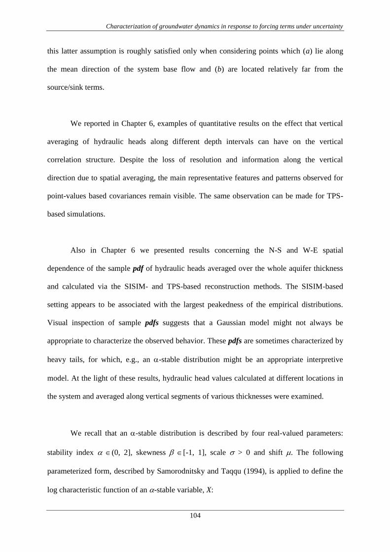
Characterization of groundwater dynamics in response to forcing terms under uncertainty
104
this latter assumption is roughly satisfied only when considering points which (a) lie along
the mean direction of the system base flow and (b) are located relatively far from the
source/sink terms.
We reported in Chapter 6, examples of quantitative results on the effect that vertical
averaging of hydraulic heads along different depth intervals can have on the vertical
correlation structure. Despite the loss of resolution and information along the vertical
direction due to spatial averaging, the main representative features and patterns observed for
point-values based covariances remain visible. The same observation can be made for TPS-
based simulations.
Also in Chapter 6 we presented results concerning the N-S and W-E spatial
dependence of the sample pdf of hydraulic heads averaged over the whole aquifer thickness
and calculated via the SISIM- and TPS-based reconstruction methods. The SISIM-based
setting appears to be associated with the largest peakedness of the empirical distributions.
Visual inspection of sample pdfs suggests that a Gaussian model might not always be
appropriate to characterize the observed behavior. These pdfs are sometimes characterized by
heavy tails, for which, e.g., an -stable distribution might be an appropriate interpretive
model. At the light of these results, hydraulic head values calculated at different locations in
the system and averaged along vertical segments of various thicknesses were examined.
We recall that an -stable distribution is described by four real-valued parameters:
stability index (0, 2], skewness [-1, 1], scale > 0 and shift . The following
parameterized form, described by Samorodnitsky and Taqqu (1994), is applied to define the
log characteristic function of an -stable variable, X:
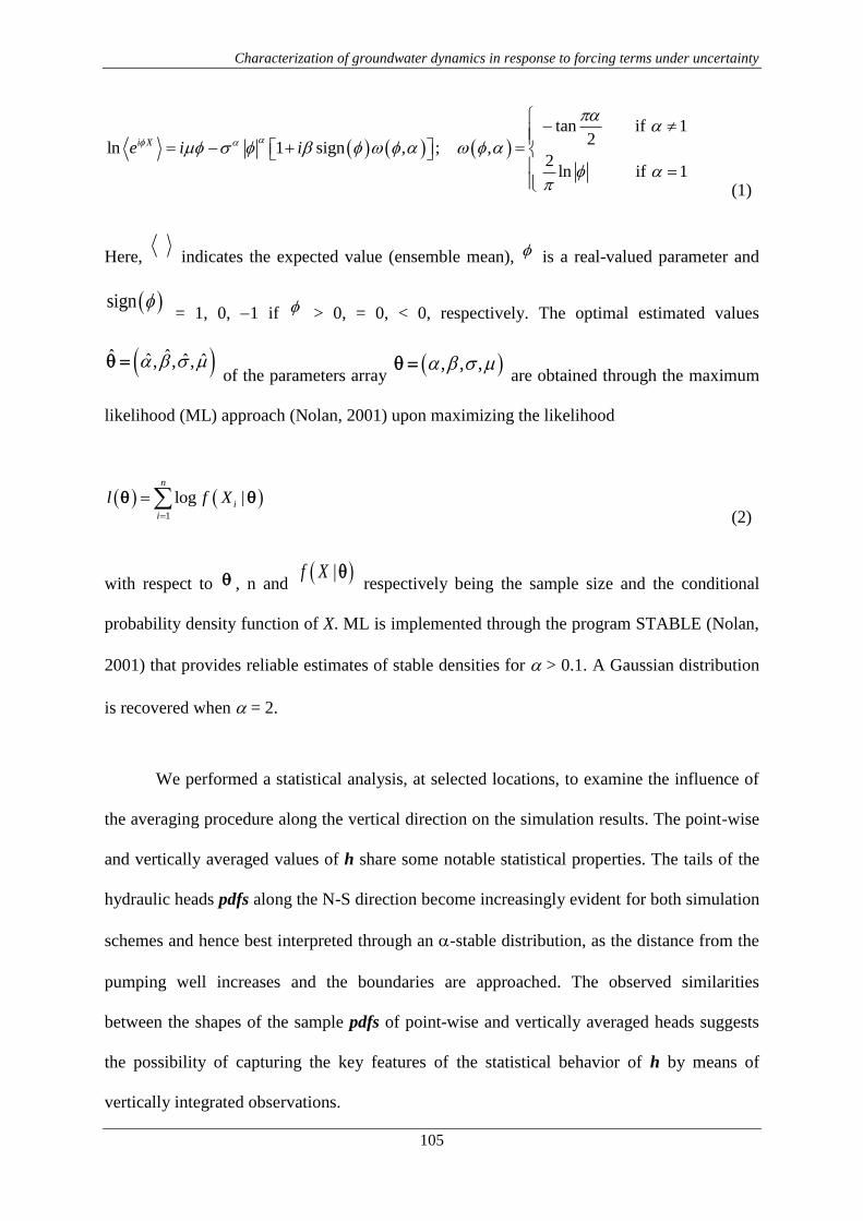
Characterization of groundwater dynamics in response to forcing terms under uncertainty
105
tan if 1
2ln 1 sign , ; ,
2ln if 1
i Xe i i
(1)
Here, indicates the expected value (ensemble mean), is a real-valued parameter and
sign = 1, 0, 1 if > 0, = 0, < 0, respectively. The optimal estimated values
ˆ ˆˆ ˆ ˆ, , , of the parameters array
, , , are obtained through the maximum
likelihood (ML) approach (Nolan, 2001) upon maximizing the likelihood
1
log |n
i
i
l f X
(2)
with respect to , n and |f X
respectively being the sample size and the conditional
probability density function of X. ML is implemented through the program STABLE (Nolan,
2001) that provides reliable estimates of stable densities for > 0.1. A Gaussian distribution
is recovered when = 2.
We performed a statistical analysis, at selected locations, to examine the influence of
the averaging procedure along the vertical direction on the simulation results. The point-wise
and vertically averaged values of h share some notable statistical properties. The tails of the
hydraulic heads pdfs along the N-S direction become increasingly evident for both simulation
schemes and hence best interpreted through an -stable distribution, as the distance from the
pumping well increases and the boundaries are approached. The observed similarities
between the shapes of the sample pdfs of point-wise and vertically averaged heads suggests
the possibility of capturing the key features of the statistical behavior of h by means of
vertically integrated observations.

Characterization of groundwater dynamics in response to forcing terms under uncertainty
106
The results introduced by Figure 6.5.5.a show that in general:
The tails of the head distributions are longer for TPS- than for SISIM- based
simulations and that they decrease as the distance from the prescribed
(deterministic) head boundaries increases.
For large distances from the prescribed flow boundaries or close to the
pumping well the distributions tends to become Gaussian (i.e., = 2.0).
At locations close to the fixed head boundaries, the distribution is skewed
towards values which are representative of the inner portion of the domain.
The pdfs of vertically averaged heads along the W-E direction appear to be
well interpreted by the Gaussian model (i.e., 2.0), regardless the
thickness of the vertical averaging segment and the generation model adopted.
The prescribed flux boundary conditions introduce less constraints (through
the Monte Carlo realizations) to the heads computed along the W-E direction
and the shape of the sample head distributions is not significantly modified
when approaching the boundaries.
Figure 6.5.5.b reports the N-S spatial dependence of estimates obtained for the
distribution of vertically averaged hydraulic heads for both methodologies. Since the scale
parameter is linked to the (ensemble) variability of the variable, we observe an increase of
with the distance from the fixed head boundaries. Consistently, is significantly larger
for the TPS-based results than for their SISIM counterparts.
Characterization of groundwater dynamics in response to forcing terms under uncertainty
107
7.4.2. Providing guidelines
NUMERICAL GRID
The numerical solution of the grid associated with flow (and eventually transport) can
and in some cases should be finer than the one adopted for the generation of the hydrofacies.
In particular, accurate numerical solution of flow requires a fine grid close to source/sink
terms such as wells. This is not associated with downscaling. We are stating that a generated
value of a property is representative of a given volume (or block) and, as such, is constant
within the volume itself (even if this volume cell is subdivided for an accurate solution of the
flow problem). Assignment of hard data (which in our case is just hydrofacies category) to
the finer grid employed for flow, has been accomplished the way described in Chapter 4. A
similar strategy for the setting of the numerical grid associated with the flow problem has
been adopted in previous works (e.g., Riva et al., 2006, 2008 and 2010).
SISIM vs TPS
The difference between the TPS and the SISIM reconstruction of facies and associated
LogK distribution is not only localized along the boundaries, but is distributed across the
simulated domain. An example of quantitative comparison between the two LogK
reconstructions (in terms of ensemble mean and variance) is offered in Chapter 5. Therefore,
the pdf of hydraulic heads obtained via SISIM- or TPS-based simulation are different not
only close to the boundaries.
MOMENTS’ CONVERGENCE
We think that this is related to the more structured heterogeneity which is embedded
in the conceptual model underlying the TPS scheme. Each realization in the TPS method is
constrained by the lithotype contact rule. This implies that the occurrence of a given facies at
Characterization of groundwater dynamics in response to forcing terms under uncertainty
108
a location is accompanied by the appearance of other facies in the surrounding blocks in
compliance with the contact rule selected. This would enhance the variability of proportions
across realizations, thus lowering the speed of convergence of moments. We note that this
effect is not dramatic in the setting considered, probably due to the contact rule selected,
where all facies are in contact with F1 (the most abundant, fine materials).
With reference to the stabilization of second order moments, the work of Ballio and
Guadagnini (2004) points out the need to increase by at least an order of magnitude the
number of simulations to discern some significant effects. We anticipate the computational
demand to be more severe for the stabilization of the complete pdf. Nevertheless, on the basis
of our experience, we think that the number of realizations performed allows to capture the
key points and shape (albeit not all the details) of the distributions. We further note that the
hydraulic head is a regular function, in the sense that it smoothes the high wave-number
components of hydraulic conductivity (K) spatial distribution which (in our setting) is in turn
related to facies proportion.
PDF TAIL OSCILLATIONS
It is likely that these oscillations are an artifact of the number of Monte Carlo
iterations performed. We adopted different binning strategies for the representation of the
simulation results and oscillations at the tails were always present to some extent. On the
basis of our experience, it is always difficult to stabilize all moments of a probability
distribution and there is not a universally recognized criterion to assess stability of all nodal
pdfs of state variables of interest (e.g., hydraulic heads). The problem is exacerbated for long-
tailed pdf distributions, where oscillations in the tails are visible even with a very large
number of data (such as 100,000 data as shown for example by Guadagnini et al., 2012).
Characterization of groundwater dynamics in response to forcing terms under uncertainty
109
7.4.2.1. Vulnerability issues
Probabilistic risk assessment (PRA) is a key application of stochastic hydrogeology
and relies on the characterization of the probability distribution of target state variables of
groundwater flow and transport. To the best of our knowledge, the characterization of the
probability distribution of point and vertically averaged hydraulic heads in large scale
randomly heterogeneous aquifers subject to pumping (and described by different hydrofacies
generation schemes of the kind we consider) is still lacking in the literature.
For the purpose of our work we think that a qualitative assessment based on visual
inspection of generated fields and a discussion grounded on low order-moments enables one
to grasp the key elements controlling the probabilistic distribution of the hydraulic heads.
Concerning the conclusions of our study, and the way they can inform how a given
application is approached, we highlight that a TPS-based approach can be considered as more
conservative than its SISIM-based counterpart because it renders an increased range of
variability in the collection of realizations of hydraulic heads.

Characterization of groundwater dynamics in response to forcing terms under uncertainty
110
8. Conclusions
Our work leads to the following major conclusions.
Hydraulic heads deduced from TPS-based flow simulations exhibit larger
variability than their counterparts evaluated by an SISIM-based modeling strategy.
This is a consequence of the fact that setting geological contact rules, as
considered within a TPS simulation scheme, can lead to an increased variability in
the internal architecture of hydrofacies distributions within a relatively large-scale
aquifer model of the kind we consider.
Covariance matrices and probability distributions of point and vertically averaged
values of hydraulic heads, display similar key representative features and patterns.
Therefore, typical measurements taken in screened boreholes can be used to infer
qualitative information about the correlation structure and the statistical properties
of heads. The latter can then be employed within typical Probabilistic Risk
Assessment procedures.
Probability distributions of heads close to prescribed head boundaries are skewed,
show a long tailing behavior and are accurately fitted by -stable distributions.
The tails of the distributions are longer for TPS- than for SISIM- based results.
Probability distributions of heads close to impervious boundaries or to source
terms (such as pumping wells) appear to be almost symmetric and reasonably well
interpreted by Gaussian models.
Characterization of groundwater dynamics in response to forcing terms under uncertainty
111
Due to the enhanced degree of variability displayed within the collection of
simulations and to the occurrence of long-tailed pdfs, reliance on a TPS scheme
yields a broader range of possible drawdown values for the simulated groundwater
system. As such, TPS-based results are associated with the most conservative (in
terms of extreme values) drawdown estimates which can then be related to a given
threshold probability of occurrence in the context of PRA protocols where the
target environmental metric is the piezometric drawdown.
8.1. Future work
Intuitively a further step towards enriching the current stage of research would be
exploring the effect of other commonly used geostatistical algorithms/techniques/procedures
on the hydraulic heads pdfs. Ideally they should treat natural heterogeneity in a similar way
(pixel-based methods) likewise the two explored models, allowing to condition the stochastic
simulations by means of hard and/or soft data of the kind presented in our study (i.e.
lithological information, extracted from a borehole network). Among the interesting available
schemes, Transition Probabilities would be an appropriate choice.
Choosing to simulate a bigger area, and a thicker groundwater system, would improve
the aim of characterizing aquifer vulnerability. Especially relevant is the cell size (that should
be decreased in the three space dimensions), as well as the interesting effect of introducing
more wells in the simulation domain. In the real double aquifer system, the existing aquitard
plays a crucial role. The aforementioned structure separates the shallow aquifer, polluted
from agricultural fertilizers, from the deeper almost pristine aquifer (preventing a fatal link)
used mainly for irrigation and drinking purposes. In other words, the aquitard protects the
confined aquifer while feeding the overlying natural springs’ network. So it appears to be of

Characterization of groundwater dynamics in response to forcing terms under uncertainty
112
paramount importance to characterize the spatial variability of the aquitard, in terms of
lateral/vertical continuity and thickness. Capturing potential discontinuities in the aquitard
would be useful to predict vulnerable locations where would be recommended to avoid
further drilling of boreholes that might end polluting the confined water body by means of
connecting vertically both water reservoirs.
Another limitation of our model is the use of stationary facies volumetric proportions
across the full domain. Vertical and lateral variability of a given hydrofacies needs to be
studied in detail by the modeler. Special attention and care are required, since vertical and
lateral resolution of our conditioning data are not the same, being the former higher than the
latter. Having built a simpler model does not subtract validity to our results. The model could
be improved by subdividing the simulated volume into regions with vertically variable
lithotype proportions (we do refer the reader to works carried out by Deraisme and Farrow,
2004; Riquelme et al., 2008 and Emery et al., 2008) and/or varying locally the truncation or
lithotype rules (Fontaine and Beucher, 2006). Even a more realistic approach would require
varying laterally the hydrofacies volumetric proportions. The hard data is out there and the
implementation of the aforesaid procedure is feasible and therefore doable.
There is typically conceptual uncertainty associated with the selection of a model
which can represent the heterogeneity of an aquifer at different scales of observation. Here,
we are interested in an observation window which encompasses horizontal and vertical length
scales of the order of 4000 and 100 m, respectively. At these scales the distribution of
lithotypes in the system is a key driver for the distribution of groundwater flow quantities. On
the other hand, the spatial heterogeneity of hydraulic parameters within a given lithotype is
relevant at smaller scales of observation as seen, for example, in the works of Winter et al.

Characterization of groundwater dynamics in response to forcing terms under uncertainty
113
(2003), and Riva et al. (2006, 2008, 2010). Treating both sources of uncertainty (i.e.,
uncertainty in the location of the boundaries between different materials and in the
distribution of attributes within each material) can be performed, e.g., in a composite medium
framework, along the lines of the references cited above. Here, we are indeed adopting a
composite medium approach where facies distribution is uncertain and hydraulic attributes
are deterministically known. Therefore, working at a smaller scale, additional realism and
consequently more complexity can be added to the model by embedding non-stationary
hydraulic conductivity (K) values for each simulated lithofacies. A set of tools and techniques
exist and could be applied in order to achieve the suggested enhancement (see works cited
above).
Last but not least a study on hydrofacies connectivity, of the kind conducted by
Knudby and Carrera (2005), would be an option to extend the work to characterize the
aquitard in the real aquifer system. We think that such a study should be aimed at providing
quantitative assessment of the relationship between such indicators and the shape and
parameters of the probability distribution of groundwater flow state variables, e.g. hydraulic
heads. The result of such an analysis on fields which are conditional on data, including
geological information which is embodied in the contact rules required for the application of
the TPS approach, would depend on the amount and location of the abovementioned data. As
a consequence, we do think that this type of quantitative analysis and exploration would
deserve a separate work, most likely to be performed on the basis of synthetic scenarios
associated with different variogram parameters and types of contact rules.

Characterization of groundwater dynamics in response to forcing terms under uncertainty
114
9. Annexes / Appendixes
In the following we present a list of published material as a direct and/or indirect
outcome of the current Ph.D. thesis and a set of dissemination activities carried out to spread
the word of the current research activity.
9.1. Publications
Perulero Serrano, R.; Guadagnini, L.; Riva, M.; Giudici, M. and Guadagnini,
A. “Impact of two geostatistical hydrofacies simulation strategies on head statistics
under non-uniform groundwater flow”. Journal of Hydrology, Volume 508, 16
January 2014, Pages 343-355.
http://dx.doi.org/10.1016/j.jhydrol.2013.11.009
Perulero Serrano, R.; Guadagnini, L.; Giudici, M., Guadagnini, A. And Riva,
M. “Application of the Truncated Plurigaussian method to delineate hydrofacies
distribution in heterogeneous aquifers”. Included in the Proceedings of the XIXth
International Conference, “Computational Methods in Water Resources” (17th
– 21st
June 2012, Champaign-Urbana; Illinois, USA).
http://cmwr2012.cee.illinois.edu/Papers/Special%20Sessions/Optimization%20an
d%20Uncertainty%20Analysis%20of%20Water%20Resources%20from%20a
%20Systems%20Perspective/Perulero%20Serrano.Raul.pdf

Characterization of groundwater dynamics in response to forcing terms under uncertainty
115
9.2. Dissemination activities
9.2.1. Conferences and workshops
IMVUL 2nd
Annual Meeting; Barcelona, SPAIN; 2010
Summer School in Flow and transport in porous media; Cargèse, Corsica,
FRANCE; 2010.
IMVUL 3rd Annual Meeting; Trondheim, Norway; 2011,
IMVUL Network Conference hosted by UPMC-Sisyphe; Groundwater
Vulnerability – Emerging Issues and New Approaches; 9th
– 12th
July, 2012;
Paris, France.
XIXth
International Conference on Computational Methods in Water
Resources; 17th
– 21st June, 2012; University of Illinois, Champaign-Urbana,
USA.
9.2.2. Posters at international conferences
Perulero Serrano, R.; Riva, M. and Guadagnini, A. “Delineation of geologic
facies in heterogeneous aquifers by the Truncated Plurigaussian Method”. It was
presented at the International Conference EGU 2011 (Vienna, Austria), in the Poster
Programme HS8.2.1. (“Stochastic Groundwater Hydrology”).
Perulero Serrano, R.; Guadagnini, L.; Giudici, M., Guadagnini, A. and Riva,
M. “Delineation of geologic facies in heterogeneous aquifers using the Truncated
Plurigaussian method: a real case study in northern Italy”. Presented at XIXth
International Conference, “Computational Methods in Water Resources” (17th
– 21st
June 2012, Champaign-Urbana; Illinois, USA).

Characterization of groundwater dynamics in response to forcing terms under uncertainty
116
9.2.3. Oral presentations
Perulero Serrano, R.; Guadagnini, A. and Riva, M. “Probability distributions
of vertically-integrated heads during a pumping test in three-dimensional
heterogeneous porous media”. Presented at IMVUL Network Conference hosted by
UPMC-Sisyphe; Groundwater Vulnerability – Emerging Issues and New Approaches;
9th
– 12th
July, 2012; Paris, France.
Perulero Serrano, R. “Probability distributions of vertically-integrated heads
during a pumping test in three-dimensional heterogeneous porous media”. Invited
presentation at “Séminaire de l'équipe hydro”, OSUR, University of Rennes 1 (8th
November 2012; Rennes, France).

Characterization of groundwater dynamics in response to forcing terms under uncertainty
117
9.3. Appendix to Chapter 7
We include in this appendix the additional material referred in Chapter 7. We did
calculate the horizontal covariance matrices of h at several lines (i.e. rows/columns along the
N-S and W-E directions) across the simulation domain. We performed point-wise (at three
different depths, namely: top, middle and bottom layers) and full vertically averaged
calculations. We repeated this procedure along various straight lines, both parallel and
perpendicular to the main flow direction, as well as at different distances from the pumping
well (which is placed, approximately, in the middle of the domain).
Moreover, to assess the impact of the correlation scale, we performed the same
covariance calculation and afterwards we divided it by the variance of the reference point.
This was done only for the full vertically averaged case.
Here we present the results corresponding to the lines that pass through the pumping
well location, along the N-S and the W-E directions. The aforementioned analyses revealed
that (integrated and point-wise) hydraulic head values display an increased degree of
horizontal correlation along the direction perpendicular to mean flow and when an SISIM
rather than a TPS approach is used.

Characterization of groundwater dynamics in response to forcing terms under uncertainty
118
Figure 9.3.1: Covariance matrices calculated along the horizontal direction, of point values of hydraulic heads at different depths (a-c and e-g) and full vertically
averaged (d, h) taken along the N-S line passing through the pumping well (see Figure 6.2.1). Namely: top layer (a, e), middle layer (b, f) and bottom layer (c, g).
Results (a-d) correspond to the SISIM-based results whereas the plots (e-h) correspond to the TPS counterparts. “Var” stands for variance.
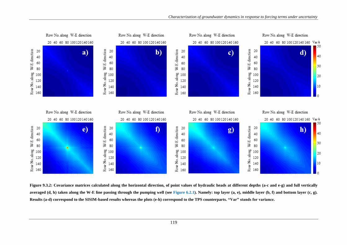
Characterization of groundwater dynamics in response to forcing terms under uncertainty
119
Figure 9.3.2: Covariance matrices calculated along the horizontal direction, of point values of hydraulic heads at different depths (a-c and e-g) and full vertically
averaged (d, h) taken along the W-E line passing through the pumping well (see Figure 6.2.1). Namely: top layer (a, e), middle layer (b, f) and bottom layer (c, g).
Results (a-d) correspond to the SISIM-based results whereas the plots (e-h) correspond to the TPS counterparts. “Var” stands for variance.
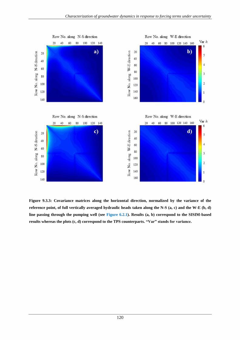
Characterization of groundwater dynamics in response to forcing terms under uncertainty
120
Figure 9.3.3: Covariance matrices along the horizontal direction, normalized by the variance of the
reference point, of full vertically averaged hydraulic heads taken along the N-S (a, c) and the W-E (b, d)
line passing through the pumping well (see Figure 6.2.1). Results (a, b) correspond to the SISIM-based
results whereas the plots (c, d) correspond to the TPS counterparts. “Var” stands for variance.
Characterization of groundwater dynamics in response to forcing terms under uncertainty
121
10. References
Ababou, R., McLaughlin, D., Gelhar, L.W. and Tompson, A. F. B., 1989. Numerical
simulation of three-dimensional saturated flow in randomly heterogeneous porous
media. Transport Porous Med. 4, 6, 549-565.
Ballio, F., and Guadagnini, A., 2004. Convergence assessment of numerical Monte Carlo
simulations in groundwater hydrology. Water Resour. Res. 40, W04603,
doi:10.1029/2003WR002876.
Bellin, A., Tonina, D., 2007. Probability density function of non-reactive solute concentration
in heterogeneous porous formations. J. Contam. Hydrol. 94, 1-2, 109-125, doi:
10.1016/j.jconhyd.2007.05.005.
Betzhold, J., Roth, C., 2000. Characterizing the mineralogical variability of a Chilean copper
deposit using plurigaussian simulations. J. S. Afr. Inst. Min. Metall. 100, 2, 111-119.
Bianchi Janetti, E., Guadagnini, L., Riva, M., Larcan, E., Guadagnini, A., 2011. Geostatistical
characterization of a regional scale sedimentary aquifer, in: F. Ubertini, E. Viola, S.
de Miranda and G. Castellazzi (Eds.), Prof. of XX Congresso dell’Associazione
Italiana di Meccanica Teorica e Applicata, Bologna 12-15 September 2011; ISBN
978-88-906340-1-7 (online), pp. 1-10.
Bolster, D., Barahona, M., Dentz, M., Fernández-García, D., Sánchez-Vila, X., Trinchero, P.,
Valhondo, C., Tartakovsky, D. M., 2009. Probabilistic risk analysis of groundwater
remediation strategies. Water Resour. Res. 45, doi: 10.1029/2008WR007551
Carle, S. F., 1999. T-PROGS: transition probability geostatistical software version 2.1.
University of California, Davis, CA.
Casar-González, R., 2001. Two procedures for stochastic simulation of vuggy formations.
SPE Paper 69663, SPE, Richardson, TX.

Characterization of groundwater dynamics in response to forcing terms under uncertainty
122
Clark, I., 1979. Practical Geostatistics. Applied Science Publishers, Barking, Essex. 129p.
Dagan, G., 1985. A note on higher-order corrections of the head covariances in steady aquifer
flow. Water Resour. Res. 21, 4, 573-578.
Dagan, G., 1989. Flow and Transport in Porous Formations. Springer-Verlag, New York.
De Barros, F. P. J., Ezzedine, S. and Rubin, Y., 2012. Impact of hydrogeological data on
measures of uncertainty, site characterization and environmental performance metrics.
Adv. Water Resour. 36, 51-64. doi: 10.1016/j.advwatres.2011.05.004.
Dell’Arciprete, D., Bersezio, R., Felletti, F., Giudici, M., Comunian, A., Renard, P., 2012.
Comparison of three geostatistical methods for hydrofacies simulation: a test on
alluvial sediments. Hydrogeol. J. 20, 299-311, doi: 10.1007/s10040-011-0808-0.
Deraisme, J. and Farrow, D., Geostatistical Simulation Techniques applied to kimberlite
orebodies and risk assessment of sampling strategies. 7th
Geostatistics Congress,
Banff, 2004.
Deutsch, C. V., Journel, A. G., 1997. GSLIB: Geostatistical software library and user’s guide,
second ed. Oxford University Press, UK.
Dowd, P., Xu, C., Mardia, K. V., Fowell, R. J., 2007. A comparison of methods for the
stochastic simulation of rock fractures. Math. Geol. 39, 7, 697-714.
Emery, X., 2004. Properties and limitations of sequential indicator simulation. Stoch. Env.
Res. Risk. A. 18, 414-424.
Emery, X., 2007. Simulation of geological domains using the plurigaussian model: New
developments and computer programs. Comput. Geosci. 33, 1189-1201.
Emery, X., Ortiz, J. M., and Cáceres, A. M., 2008. Geostatistical modeling of rock type
domains with spatially varying proportions: Application to a porphyry copper deposit.
Journal of the South African Institute of Mining and Metallurgy, vol. 108, n. 5, pp.
285-292.
Characterization of groundwater dynamics in response to forcing terms under uncertainty
123
Englert, A., Vanderborght, J. & Vereecken, H., 2006. Prediction of velocity statistics in three-
dimensional multi-Gaussian hydraulic conductivity fields. Water Resour. Res. 42, 3,
W03418, doi: 10.1029/2005WR004014.
Enzenhoefer, R., Nowak, W., Helmig, R., 2012. Probabilistic exposure risk assessment with
advective dispersive well vulnerability criteria. Adv. Water Resour. 36, 121-132, doi:
10.1016/j.advwatres.2011.04.018.
Falivene, O., Arbués, P., Gardiner, A., Pickup, G., Muñoz, J.A., Cabrera, L., 2006. Best
practice stochastic facies modeling from a channel-fill turbidite sandstone analog (the
Quarry outcrop, Eocene Ainsa basin, northeast Spain). AAPG Bull., 90, 1003-1029.
Falivene, O., Cabrera, L., Muñoz, J. A., Arbués, P., Fernández, O., Sáez, A., 2007. Statistical
grid-based facies reconstruction and modeling for sedimentary bodies. Alluvial-
palustrine and turbiditic examples. Geol. Acta. 5, 199-230.
Fiorotto, V., Caroni, E., 2002. Solute concentration statistics in heterogeneous aquifers for
finite Peclet values. Transport Porous Med. 48, 3, 331-351, doi:
10.1023/A:1015744421033.
Fontaine, L. and Beucher, H. 2006. Simulation of the Muyumkum uranium roll front deposit
by using truncated plurigaussian method. In 6th international mining geology
conference, Darwin.
Galli, A. G., Beucher, H., Le Loc’h, G., Doligez, B., Heresim group, 1994. The Pros and
Cons of the truncated Gaussian method, in: Armstrong, M., Dowd, P. A., (Eds.),
Geostatistical Simulations. Kluwer Academic Publishers, Netherlands, pp. 217-233.
Gandolfi, C., Ponzini, G. and Giudici, M., 2007. Realizzazione di un modello preliminare del
flusso idrico nel sistema acquifero della Provincia di Cremona.
Characterization of groundwater dynamics in response to forcing terms under uncertainty
124
Guadagnini, A., Neuman, S. P., 1999a. Nonlocal and localized analyses of conditional mean
steady state flow in bounded, randomly nonuniform domains 2. Computational
examples. Water Resour. Res. 35, 10, 2999-3018, doi: 10.1029/1999WR900159.
Guadagnini, A., Neuman, S. P., 1999b. Nonlocal and localized analyses of conditional mean
steady state flow in bounded, randomly nonuniform domains 1. Theory and
computational approach. Water Resour. Res. 35, 10, 2999-3018, doi:
10.1029/1999WR900160.
Guadagnini, A., Riva, M., Neuman, S. P., 2003. Three-dimensional Steady State Flow to a
Well in a Randomly Heterogeneous Bounded Aquifer. Water Resour. Res. 39(3)
1048, doi: 10.1029/2002WR001443.
Guadagnini, A., Neuman, S. P., Riva, M., 2012. Numerical Investigation of Apparent
Multifractality of Samples from Processes Subordinated to Truncated fBm. Hydrol.
Process. 26, 19, 2894-2908, doi: 10.1002/hyp.8358.
Guadagnini, L. et al. “Modello quali-quantitativo per la tutela della ‘Fascia dei Fontanili’
nella fase di pianificazione della risorsa acqua”. Relazione tecnica; January 2007–
December 2008.
Hernández, A. F.,. Neuman, S. P., Guadagnini, A., Carrera, J., 2006. Inverse stochastic
moment analysis of steady state flow in randomly heterogeneous media. Water
Resour. Res. 42, W05425, doi:10.1029/2005WR004449.
Isaaks, E. H., Srivastava, R. M., 1989. An Introduction to Applied Geostatistics. N.Y.: OUP.
561p.
Jones, L., 1990. Explicit Monte Carlo Simulation Head Moment Estimates for Stochastic
Confined Groundwater Flow. Water Resour. Res. 26, 6, 1145-1153, doi:
10.1029/WR026i006p01145.
Characterization of groundwater dynamics in response to forcing terms under uncertainty
125
Journel, A. G., Alabert, F. G., 1989. Non-Gaussian data expansion in the earth sciences. Terra
Nova, 1, 123-134.
Jurado, A., De Gaspari, F., Vilarrasa, V., Bolster, D., Sánchez-Vila, X., Fernández-García,
D., Tartakovsky, D. M., 2012. Probabilistic analysis of groundwater-related risks at
subsurface excavation sites. Eng. Geol.. 125, 35-44, doi:
10.1016/j.enggeo.2011.10.015.
Kitanidis, P. K., 1997. Introduction to Geostatistics. Applications in Hydrogeology.
Cambridge, New York, Port Chester, Melbourne, Sydney: Cambridge University
Press. 249 pp.
Kunstmann, H., Kastens, M., 2006. Determination of stochastic well head protection zones
by direct propagation of uncertainties of particle tracks. J. Hydrol. 323, 1-4, 215-229,
doi: 10.1016/j.jhydrol.2005.09.003.
Lee, S-Y., Carle, S. F., Fogg, G. E., 2007. Geologic heterogeneity and a comparison of two
geostatistical models: sequential Gaussian and transition probability-based
geostatistical simulation. Adv. Water Resour. 30, 1914-1932.
Maione, U., Paoletti, A., Grezzi, G., 1991. Studio di gestione coordinata delle acque di
superficie e di falda nel territorio compreso fra i fiumi Adda e Oglio e delimitato dalle
Prealpi e dalla linea settentrionale di affioramento dei fontanili
Mariethoz, G., Renard, Ph., Cornaton, F., Jaquet, O., 2009. Truncated Plurigaussian
Simulations to Characterize Aquifer Heterogeneity. Ground Water. 47, 13-24.
McDonald, M.G., Harbaugh, A.W., 1988. A modular three-dimensional finite-difference
ground-water flow model. Techniques of Water-Resources Investigations of the
United States Geological Survey, Book 6, Chapter A1.

Characterization of groundwater dynamics in response to forcing terms under uncertainty
126
Nolan, J. P., 2001. Maximum likelihood estimation of stable parameters. In: O. E. Barndorff-
Nielsen, T. Mikosch, and S. I. Resnick (Eds.), Levy Processes:Theory and
Applications, Boston: Birkhäuser, pp 379-400.
Nowak, W., Schwede, R. L., Cirpka, O. A., Neuweiler, I., 2008. Probability density functions
of hydraulic head and velocity in three-dimensional heterogeneous porous media.
Water Resour. Res. 44, W08452, doi: 10.1029/2007WR006383.
Osnes, H., 1995. Stochastic analysis of head spatial variability in bounded rectangular
heterogeneous aquifers. Water Resour. Res. 31, 12, 2981-2990.
Rametta, D. (2008). Interazione tra reticolo idrografico superficiale e acquifero sotterraneo
nella modellistica idrologica distribuita, Politecnico di Milano, Milano.
Remy, N., Alexandre, B., Jianbing, W., 2009. Applied Geostatistics with SGeMS: A user’s
guide. 1st ed. Cambridge University Press; doi: 10.1017/CBO9781139150019.
Riquelme Tapia, R., Le Loc'H G., Carrasco Castelli, P., 2008. Truncated gaussian and
plurigaussian simulations of lithological units in Mansa Mina deposit. VIII
International Geostatistics Congress, GEOSTATS 2008, Santiago: Chile (2008).
Riva, M., Guadagnini, L., Guadagnini, A., Ptak, T., Martac, E., 2006. Probabilistic study of
well capture zones distribution at the Lauswiesen field site. J. of Cont. Hydrol. 88, 92-
118.
Riva, M., Guadagnini, A., Fernández-García, D., Sánchez-Vila, X., Ptak, T., 2008. Relative
importance of geostatistical and transport models in describing heavily tailed
breakthrough curves at the Lauswiesen site. J. Contam. Hydrol. 101, 1-13.
Riva, M., Guadagnini, A., 2009. Effects of evolving scales of heterogeneity on hydraulic
head predictions under convergent flow conditions. Hydrogeol. J., 17, 817-825,
doi:10.1007/s10040-008-0396-9.
Characterization of groundwater dynamics in response to forcing terms under uncertainty
127
Riva, M., Guadagnini, L., Guadagnini, A., 2010. Effects of uncertainty of litho-facies,
conductivity and porosity distributions on stochastic interpretations of a field-scale
tracer test. Stoch. Env. Res. Risk. A. 24, 955-970, doi: 10.1007/s00477-010-0399-7.
Rubin, Y., and Dagan, G., 1988. Stochastic analysis of boundaries effects on head spatial
variability in heterogeneous aquifers: 1. Constant head boundary. Water Resour. Res.
24, 10. 1689-1697.
Rubin, Y., and Dagan, G., 1989. Stochastic analysis of boundaries effects on head spatial
variability in heterogeneous aquifers: 2. Impervious boundary. Water Resour. Res. 25,
4, 707-712.
Samorodnitsky, G., Taqqu, M., 1994. Stable Non-Gaussian Random Processes. New York:
Chapman and Hall.
Scheibe, T.D., Murray, C.J., 1998. Simulation of geologic patterns: a comparison of
stochastic simulation techniques for groundwater transport modelling. In: Fraser GS,
Davis JM (eds) Special publication of the SEPM (Society for Sedimentary Geology),
Tulsa, OK, 107-118.
Schwede, R. L., Cirpka, O. A., Nowak, W., Neuweiler, I., 2008. Impact of sampling volume
on the probability density function of steady state concentration. Water Resour. Res.
44, 12, doi: 10.1029/2007WR006668.
Strebelle, S., 2002. Conditional simulation of complex geological structures using multiple
point statistics. Math. Geosci. 34, 1-22.
Tartakovsky, D. M., 2013. Assessment and management of risk in subsurface hydrology: A
review and perspective. Adv. Water Resour., 51, 247-260, doi:
10.1016/j.advwatres.2012.04.007.

Characterization of groundwater dynamics in response to forcing terms under uncertainty
128
Vassena, C., Rienzner, M., Ponzini, G., Giudici, M., Gandolfi, C., Durante, C., Agostani, D.,
2012. Modeling water resources of a highly irrigated alluvial plain (Italy): calibrating
soil and groundwater models. Hydrogeol. J. 20, 3, 449-467, doi: 10.1007/s10040-011-
0822-2.
Xu, C., Dowd, P. A., Mardia, K. V., Fowell, R. J., 2006. A flexible true plurigaussian code
for spatial facies simulations. Comput. Geosci. 32, 1629-1645.
Winter, C. L, Tartakovsky, D. M., Guadagnini, A., 2003. Moment differential equations for
flow in highly heterogeneous porous media. Surveys in Geophysics, 24(1), 81-106.
Wu, J., Boucher, A., Zhang, T., 2008. SGeMS code for pattern simulation of continuous and
categorical variables: FILTERSIM. Computers & Geosciences. 34, 728, 1863-1876.
Zarlenga, A., Fiori, A., Soffia, C., and Jankovic, I., 2012. Flow velocity statistics for uniform
flow through 3D anisotropic formations. Adv. Water Resour. 40, 37-45.
Zhang, T., Switzer, P., Journel, A. G., 2006. Filter-based classification of training image
patterns for spatial simulation Math. Geosci. 38, 63-80.