Characterization and optimization of CERN Secondary ...

CONSEIL EUROPEEN POUR LA RECHERCHE NUCLEAIRE

UNIVERSITAT POLITECNICA DE CATALUNYA

Characterization and optimization of CERN

Secondary Emission Monitors (SEM) used for

beam diagnostics.

BACHELOR DEGREE IN PHYSICS ENGINEERINGFINAL DEGREE PROJECT

by

Araceli Navarro Fernandez

Supervisors:Dr. Federico Roncarolo CERN, GeneveDr. Jordi Llorca UPC, Barcelona

May 2017

Abstract

The European Organization for Nuclear Research, more commonly known as CERN, isone of the world’s most influential particle physics center. The organization is based in anorthwest suburb of Geneva, on the Franco-Swiss border and has 22 member states. AtCERN, people with different backgrounds from all around the world work together in orderto understand, among other things, the fundamental structure of the universe. To do that,particles have to be accelerated up to extremely high energies in a controlled and safe way.

This work has been carried out within the BE-BI-PM section, responsible of the beamdiagnostics instruments that allow the observation of the transverse profiles of particle beams.Different instruments and techniques are used for this purpose but in the following pagesonly the monitors based on Secondary Electron Emission (SEE) phenomena will be tackled.After introducing the physics behind Secondary Emission Monitors (SEM), their performanceand limitations will be discussed. This will be based on simulations and beam experimentsperformed during the thesis work, mostly related to the LINAC4 , a new linear acceleratorjust completed at CERN.

The first part of this document contains an introduction to the CERN accelerator chain,with particular emphasis on LINAC4 .

Chapter 2 focuses on various aspects of the particles interaction with matter, which areused to define the theory behind SEE, the main process behind the SEM’s signal generation.

Chapter 3 starts presenting some examples of SEM detectors, focusing on SEM grids andWire Scanners. This is followed with a practical example in which SEM grids were used inorder to understand the flawed Beam Current Transformers (BCT) measurement of the beamtransmission along the linac.

Chapter 4 explains the theory defining the thermal impact of particles interacting withmatter. Such a theory was used to simulate the heating of SEMs during their operation.

Chapter 5 introduces the concept of beam emittance and how SE detectors can be usedfor its estimation. This explanation is again presented with a practical example of emittancemeasurement in the LINAC4 3 MeV Test Stand. Chapter 6 gives some insights on the physicsbehind electron stripping and CFI injection, followed with the description of the strippingsystem that will be installed at the exit of LINAC4 in order to inject protons into the ProtonSynchrotron Booster (PSB). The main part of this chapter will present the experimentalresults of a series of experiments performed at the LINAC4 Half Sector Test (HST) facilityby means of the H0/H− monitors.

1

Contents

Abstract . . . . . . . . . . . . . . . . . . . . . . . . . . . . . . . . . . . . . . . . . . 1

Introduction 3CERN Accelerator Complex . . . . . . . . . . . . . . . . . . . . . . . . . . . . . . . 3LINAC4 Project . . . . . . . . . . . . . . . . . . . . . . . . . . . . . . . . . . . . . 4

Interaction of particles with matter 5Energy loss by interaction with electrons . . . . . . . . . . . . . . . . . . . . . . . . 5The Bethe-Bloch theory and Range . . . . . . . . . . . . . . . . . . . . . . . . . . . 6Secondary Electron Theory . . . . . . . . . . . . . . . . . . . . . . . . . . . . . . . 8SEY Dependence with angle of incidence . . . . . . . . . . . . . . . . . . . . . . . . 10Delta Rays . . . . . . . . . . . . . . . . . . . . . . . . . . . . . . . . . . . . . . . . 10Backscattering . . . . . . . . . . . . . . . . . . . . . . . . . . . . . . . . . . . . . . 11Multiple Coulomb Scattering . . . . . . . . . . . . . . . . . . . . . . . . . . . . . . 11

Secondary Emission Monitors (SEM) 13Wire Grids . . . . . . . . . . . . . . . . . . . . . . . . . . . . . . . . . . . . . . . . 13Wire Scanners . . . . . . . . . . . . . . . . . . . . . . . . . . . . . . . . . . . . . . 14Other Secondary Emission Monitors . . . . . . . . . . . . . . . . . . . . . . . . . . 15Signal Generation in SEM. . . . . . . . . . . . . . . . . . . . . . . . . . . . . . . . 15Profile monitoring with SEM grids . . . . . . . . . . . . . . . . . . . . . . . . . . . 16Emittance growth due to Multiple Coulomb Scattering . . . . . . . . . . . . . . . . 18

Study of the beam induced wire heating 20Wire Heating . . . . . . . . . . . . . . . . . . . . . . . . . . . . . . . . . . . . . . . 20Radiative Cooling . . . . . . . . . . . . . . . . . . . . . . . . . . . . . . . . . . . . 20Thermoionic Cooling . . . . . . . . . . . . . . . . . . . . . . . . . . . . . . . . . . . 21Thermal Conduction . . . . . . . . . . . . . . . . . . . . . . . . . . . . . . . . . . . 22Temperature simulations . . . . . . . . . . . . . . . . . . . . . . . . . . . . . . . . . 23

Transverse beam emittance and Slit-Grid system measurements 25Basics of Beam Dynamics and Phase Space . . . . . . . . . . . . . . . . . . . . . . 25Emittance measurement with Slit-Grid system . . . . . . . . . . . . . . . . . . . . 27Emittance measurements at 3MeV Test Stand . . . . . . . . . . . . . . . . . . . . . 27Emittance measurements accuracy . . . . . . . . . . . . . . . . . . . . . . . . . . . 29

LINAC4 ’s H0H− Monitors 33Charge Exchange Injection (CEI) . . . . . . . . . . . . . . . . . . . . . . . . . . . . 33Stripping Foil . . . . . . . . . . . . . . . . . . . . . . . . . . . . . . . . . . . . . . . 34H0H− Monitors in PSB HST . . . . . . . . . . . . . . . . . . . . . . . . . . . . . . 35Electronics conceptual design and available signals. . . . . . . . . . . . . . . . . . . 37Measurements procedure. . . . . . . . . . . . . . . . . . . . . . . . . . . . . . . . . 38Oasis Signals and first conclusions. . . . . . . . . . . . . . . . . . . . . . . . . . . . 39Digitized signals and calibration factor. . . . . . . . . . . . . . . . . . . . . . . . . 41Reliability of k factor for H0 signals. . . . . . . . . . . . . . . . . . . . . . . . . . . 42

Conclusions 46

2

Chapter 1

Introduction

CERN Accelerator Complex

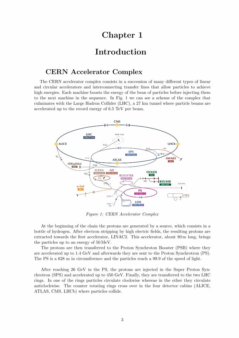
The CERN accelerator complex consists in a succession of many different types of linearand circular accelerators and interconnecting transfer lines that allow particles to achievehigh energies. Each machine boosts the energy of the bean of particles before injecting themto the next machine in the sequence. In Fig. 1 we can see a scheme of the complex thatculminates with the Large Hadron Collider (LHC), a 27 km tunnel where particle beams areaccelerated up to the record energy of 6.5 TeV per beam.

Figure 1: CERN Accelerator Complex

At the beginning of the chain the protons are generated by a source, which consists in abottle of hydrogen. After electron stripping by high electric fields, the resulting protons areextracted towards the first accelerator, LINAC2. This accelerator, about 80 m long, bringsthe particles up to an energy of 50 MeV.

The protons are then transferred to the Proton Synchroton Booster (PSB) where theyare accelerated up to 1.4 GeV and afterwards they are sent to the Proton Synchrotron (PS).The PS is a 628 m in circumference and the particles reach a 99.9 of the speed of light.

After reaching 26 GeV in the PS, the protons are injected in the Super Proton Syn-chrotron (SPS) and accelerated up to 450 GeV. Finally, they are transferred to the two LHCrings. In one of the rings particles circulate clockwise whereas in the other they circulateanticlockwise. The counter rotating rings cross over in the four detector cabins (ALICE,ATLAS, CMS, LHCb) where particles collide.

3

The complex of the CERN accelerator is very versatile and far from being just the in-jectors of the LHC. Some of the machines have their own dedicated experimental areas toexplore a wide range of physics phenomena. The complexity of these machines and experi-mental areas makes it impossible to explain all of them.

In the following section we are going to give some insights of LINAC4 , which has been thecontext of all our simulations and measurements. LINAC4 was conceived to replace the oldLINAC2. Its construction and commissioning up to its to energy of 160 MeV were completedat the beginning of 2017 and its connection to the PSB is foreseen for 2019.

LINAC4 Project

The source and the linac are essential for determining the LHC beams quality, since theydetermine the maximum beam brilliance, which can be seen as the maximum density ofparticles that can be brought into collision in a collider. Such a brilliance, that after the linaccan only be deteriorated and not increased, is achieved by find the right compromise betweenmaximum beam intensity and minimum transverse/longitudinal beam dimensions.More than 10 years ago, in order to address the LINAC2 ageing and to improve the beambrilliance, it was decided to design and build L4, an H− linear accelerator, able to acceleratepulses of up to 1014 particles to 160 MeV.

Figure 2: LINAC4 schematic layout

The LINAC4 layout is shown in Fig. 2. The chosen sequence of accelerating sections isquite standard for modern pulsed linac designs. The particles are produced in the ions sourcewhich is followed by a Low Energy Beam Transport (LEBT), needed to match the beam withthe Radio Frequency Quadruple (RFQ) cavitiy. The RFQ is followed by a chopping line anda sequence of three accelerating structures. These three structures bring the energy up to 160MeV and they are a Drift Tube Linac (DTL), a Cell-Coupled Drift Tube Linac (CCDTL)and a Pi-Mode Structure (PIMS). They increase the particles’ energy up to 50 MeV, 100MeV and 160 MeV respectively. More details can be found in [1].

Along the 86 m of the new linear accelerator, a considerable amount of detectors areinstalled in order to monitor and control the beam. In the following pages we will focuson the transverse beam profile and emittance monitors, giving special attention to the SEMgrids and Wire scanners (Chapter 3) and slit-grid system (Chapter 5). More details aboutall the other LINAC4 beam diagnostics can be found in [1].

4

Chapter 2

Interaction of particles with matter

When a particle propagates through matter, it will have certain probability to interact withthe nuclei or with the electrons present in that material. The probability that the particleshave of interacting with the medium, either with the electrons or the nucleus, is representedby what is called the cross sections. The total interaction cross section will be the sum ofthe cross sections of the individual possible interactions. As we can see in Fig. 3, when acharged particle travels through matter it predominantly interacts with the electrons of themedium, either by Coulomb force interactions or collision interactions. Interactions with thecore of the nucleus are also possible (i.e. Rutherford scattering) but much less frequent. Inthe following chapter we shall focus our analysis on non-relativistic or near relativistic ionsinteracting with solid targets. Due to the range of energy we will be working on, we are goingto focus in the interactions that an incident ion has with the electrons in the medium.

Figure 3: Nuclear and electronic stopping power for protons in aluminium versus particleenergy per nucleon. From [2]

Energy loss by interaction with electrons

The incident particle or ion will transfer energy to the electrons in the solid when travelingthrough it. These electrons can be either excited to higher energy levels or gain enoughenergy to escape from the solid. As this happens, the incident particle will lose energy, mostfrequently the energy losses are small and this is usually described by the mean differentialenergy loss dE/dx (or by the stopping power S=-dE/dx). For a given incident particle andtarget, this energy loss has been found to be very dependent with the velocity of the incidentparticle. Unfortunately there is no single theorem that can describe the energy loss at allrange of energy. Depending on the energy range of the incident particle, some propertiesfrom the particle and the target become relevant. The energy loss of a muon in copper is

5

illustrated in Fig. 4. The pattern is rather complicated but allows defining three major energyranges [3]:

Energy[MeV/amu]

Gamma factorγ

Normalised momentumβγ

Framework

<10 <1.01 <0.15 Lindhard10− 106 1.01 - 1000 0.15 - 1000 Bethe - Bloch>106 >1000 >1000 Radiative Losses

Table 1: Energy range of the incident particle and its corresponding framework

In the mid-energy range the electrostatic stopping power is well defined by the Bethe-Bloch theory, which treats the exchange of energy between the incident particle and theatoms as the scattering of a charged particle from an isolated atom. At lower energies thevelocity of the incident particle becomes comparable or even lower than the target electrons’and it is required to take into account interactions between atoms as it is done with Lindhardtheory. In ultra-relativistic energy range, radiative processes such as bremsstrahlung becomethe dominant contribution to the energy loss.

Figure 4: Electronic stopping power for positive muons on copper as function of the particlekinetic energy. The solid curve represents the total stopping power From [4]

The Bethe-Bloch theory and Range

The Bethe-Boch theory describes the mean rate of energy loss (stopping power of thematerial) for energies of the incident particle from 10− 106MeV/amu and can be describedas [5]:

−dEdx

= Kz2Z

A

1

β2

[1

2ln

2mec2β2γ2TmaxI2

− β2 − δ (βγ)

2

](1)

Where Z and A are the atomic and mass number of the material. Ze is the charge ofthe particle, K/A is 0.307 MeV g−1cm2 and the δ(βγ) is a predetermined density correctionnecessary for high energetic particles, units are MeV cm2g−1. I is the mean excitation energyfor the given material, and varies from a few eV for materials with low Z to hundreds of eVfor materials with high Z and can be calculated with the empirical formula:

6

I = 16Z0.9 (2)

Tmax represents the maximum energy that can be transferred to a particle in an elasticcollision. It can be calculated as:

Tmax =2mec

2β2γ2

1 + γmec2

Mc2+(mec2

Mc2

)2 (3)

Where γ and β are the relativistic parameters, M is the mass of the projectile and me isthe electron mass.

Figure 5: Bragg peak of 100 MeV protons in Tungsten. Energy deposition increases withdistance, reaching a maximum at around 0.8 cm.

The energy deposition is not constant, it has a peak because interaction cross sectionincreases as the charged particle energy decreases. In Fig. 5, we can see an example of theBragg curve that plots the energy loss of ionizing radiation during is travel through matter.If we can just take into account the particle loses because of ionization and atomic excitationwe can define the range as the distance traveled by particles in matter until their energy is(almost) zero. The range depends on the type of particle, on its initial energy and on thematerial it goes through. For heavy particles it can be calculated integrating the Bethe-Blochformula [6]. After integration, the relation between the range and energy for particles abovefew Mev is:

R (E) ∝ E2 (4)

Therefore, the range will be greater as the energy of the particle increases. For electrons,the effect of multiple scattering induces chaotic trajectories and the range is very difficultto estimate. An excellent review of all electron range-energy was recollected by Katz andPenfold who proposed the following empirical relationship for energies from 0.01 MeV to 3MeV [6] :

R (E) = 41213

27

A

ZEn (5)

With n = 1.265 − 0.0954ln (E), E the energy of the electron, A and Z, respectively thenumber of nucleons and the atomic number of the material. R is given in mgcm2.

7

Secondary Electron Theory

When a particle passes through the interface of a material, it will transfer energy to theelectrons in the medium. Depending on the energy these electrons get, they can be excitedto a higher energy level or gain enough energy to be emitted from the material, this emissionprocess is known as Secondary Electron Emission (SEE). This is a surface effect so we canfind this effect when the particle either enters or exits the material. Usually the electrons inthe outer shells are the ones to be ionized but ionization of the inner shell is also possiblealthough less probable. The SEE process can be provided in three steps [7]:

Figure 6: Ion induced secondary electron spectra for a variety of materials. In this caseincident ions are protons at 500 keV. The integral of each curve in energy gives the totalsecondary electron yield. From [8]

The first step is the creation of the secondary electron in the bulk of the material. Theminimum energy you need for creating a SE is the one required to excite the electrons abovethe Fermi level to the conduction band. If the projectile is an ion containing electrons theseelectrons can be stripped off and also produce further ionization, but if the electrons fromthe ion are scattered off the material, they cannot be counted as secondary electrons. Thesecond step in the SEE process could be the diffusion in the material. When the secondaryelectrons travel through the material, they lose their energy. The greater the energy lose thesmaller the distance they will travel.

Finally, the last step would be the emission process. In order to be emitted the secondaryelectrons have to have enough energy to overcome the surface potential, which is characterizedwith the work function eφ, so the barrier height would be W = EF+φe, with Ef the fermi leveland φ the surface potential. The emission process is a directive phenomenon, as a consequenceapart from having enough energy the electrons must have a velocity vector laying inside aescape cone with a maximum angle θmax normal to the surface:

8

θmax = arcos

(√W

Ei

)Ei ≥W (6)

The theoretical treatment of the SEE was formulated in 1957 by E.J. Sternglass. Themain parameter describing these phenomena is the Secondary Electron Yield (SEY) whichgives an average number of electrons emitted per incident particle. It can be described bythe following numerical relation [7]:

SEY = 0.01LsdE

dx|el[1 +

1

1 + (5.4× 10−6E/Ap)

](7)

Ls =(

3.68× 10−17NZ1/3)−1

[cm] (8)

N is the number of atoms per unit volume, Z is the atomic mass of the material’s atomwhile E and Ap are the kinetic energy and the mass of the projectile. Notice that the elec-tronic energy loss, dE/dx, should be in [eV/cm] and the projectiles kinetic energy in eV.

In Fig. 6, we can find the energy distribution of the secondary electrons emitted from dif-ferent targets. N (E) is related to the total secondary electron yield through

∫N (E) dE = γ,

where γ is the total secondary electron yield. As a general trend, we can see that the sec-ondary electrons generated have an energy much smaller than the ion that has producedthem. Although the exact values of these spectra are dependent on the projectile-targetcombination, in general it is found a sharp increase at low energies followed by a maximumat several eV and a decrease towards higher energies. Simulations of this low energy electronsare more complicated due to the limiting low energy barrier of some simulation programs suchas FLUKA [9].

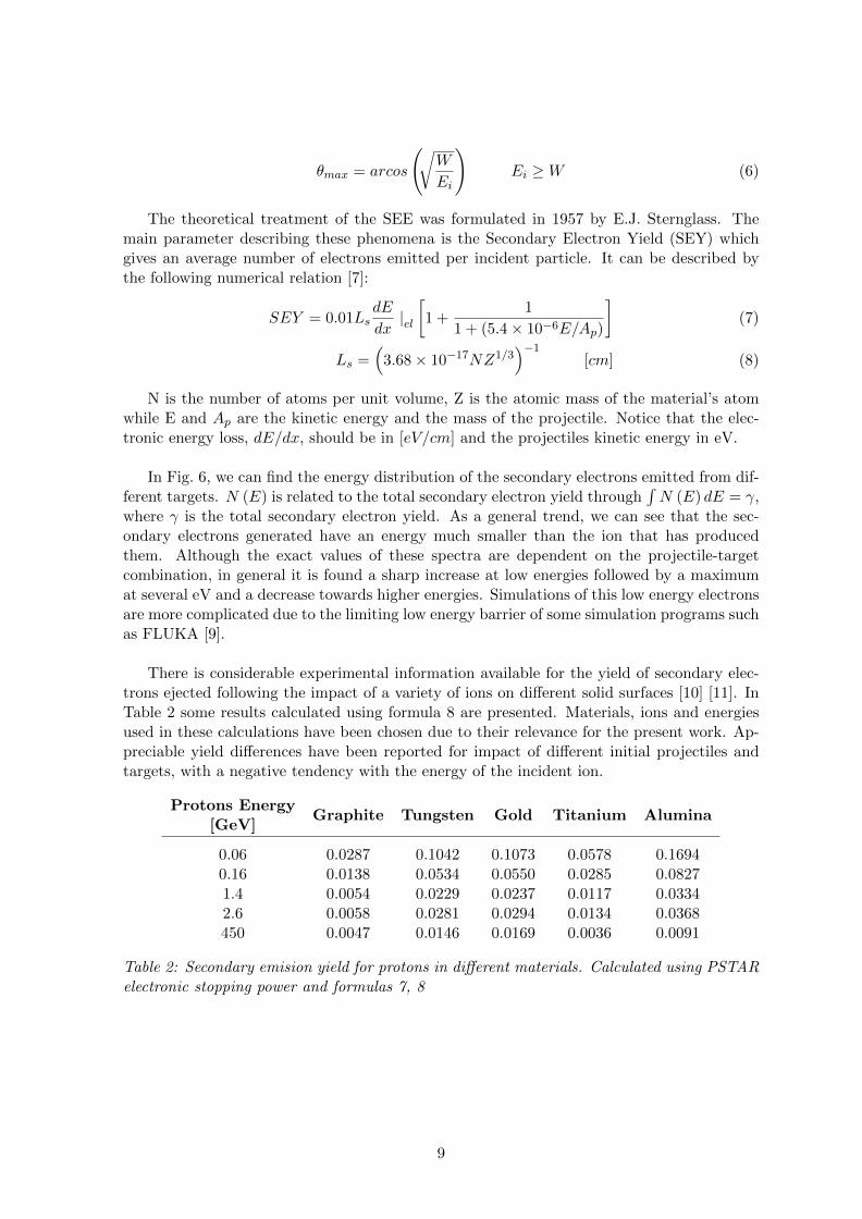
There is considerable experimental information available for the yield of secondary elec-trons ejected following the impact of a variety of ions on different solid surfaces [10] [11]. InTable 2 some results calculated using formula 8 are presented. Materials, ions and energiesused in these calculations have been chosen due to their relevance for the present work. Ap-preciable yield differences have been reported for impact of different initial projectiles andtargets, with a negative tendency with the energy of the incident ion.

Protons Energy[GeV]

Graphite Tungsten Gold Titanium Alumina

0.06 0.0287 0.1042 0.1073 0.0578 0.16940.16 0.0138 0.0534 0.0550 0.0285 0.08271.4 0.0054 0.0229 0.0237 0.0117 0.03342.6 0.0058 0.0281 0.0294 0.0134 0.0368450 0.0047 0.0146 0.0169 0.0036 0.0091

Table 2: Secondary emision yield for protons in different materials. Calculated using PSTARelectronic stopping power and formulas 7, 8

9

SEY Dependence with angle of incidence

As we mentioned before the emission process in the secondary electron generation is limitedwith the potential barrier and the need of lying inside the escape cone. We can call Ls to thethickness of the material from which the low energy electrons can escape. If the projectile hasan angle of incidence θ with respect to a perpendicular incidence to the surface, the lengthof the particle track increases by a factor 1/cos (θ). So if we just take this into account theresulting SEY would be:

SEY (θ) = SEY (θ) cos (θ)−1 (9)

Being SEY (0) the secondary emission yield for a perpendicular incidence. This formulawould be quite difficult to implement because the resulting value for grazing angles tendsto infinite. Experimental data has shown that for angles bigger than 70 deg the cosinedependence is no longer valid. Deviations are also encountered for heavier ions giving anangular dependence that can be parametrized as [12]:

SEY (θ) = SEY (θ) cos (θ)−f (10)

Equation 10 is purely empirical and for angles close to 90 deg data deviate even from thisbehavior. Realize that the bigger the angle of incidence the bigger Ls becomes, therefore themean value dE/dx cannot be considered constant. At the same time, the longer the distancethe particle goes through, the bigger the deviation from a straight line due to multiple coulombscattering.

Delta Rays

Most frequently the electrons generated by secondary emission have small energy, but ifthe energy transferred to the electron is above few hundred eV (up to Tmax) they may beable to generate secondary ionization. This high energy electrons are called delta-rays. Thenumber of delta rays generated by an incident ion which speed is β = v/c in 1 cm, inside amedium of electronic density N, can be calculated with the following formula [13]:

n (T ) =2πNe4Z2

mec2β2

(1

T− 1

Tmax

)(11)

With Z corresponding to the effective charge of the incident ion, e is the charge of theelectron and me its mass. T corresponds to the energy of the incident particle whereas Tmaxis the maximum possible kinetic energy transferred to an electron, that is formula 3. In orderto calculate the total number of delta rays, formula 11 can be integrated from some arbitrarilylower energy limit to the maximum energy delta rays can get. Our main concern in this paperis the effect of delta rays in the generation of extra secondary electron emission. In orderto have an idea of how relevant is this effect, some simulations where done. In Table 3 wepresent as an example the case of a 160 MeV proton beam. In order to calculate the numberof delta rays we had to consider a minimum threshold energy, in this case we’ve consideredas delta rays all the secondary electrons with an energy bigger than 100eV.

10

Energy160 [MeV]

delta ray perincident proton

Total SE perpulse due to proton

Total SE per pulsedue to delta rays

Carbon 0.0098 1.37e+12 2.9e+9Tungsten 0.0202 5.34e+12 4.03e+9

Table 3: Importance of delta rays in SE phenomena. Results calculated using FLUKA soft-ware for a 160 MeV proton beam filled with 1 · 1014 Protons.

Backscattering

When particles enter a material its path can be deflected from the initial direction becauseof the interactions with the material. Usually the effect results in changing the forward direc-tion of the incident particle by a few degrees, but occasionally the particle can be deflectedthrough a value of around 180 resulting in it exiting the material from the same side as itentered, these phenomena is what is known as back scattering. The back scattering probabil-ity is proportional to the Z of the material and it is also higher if the incident particle massis low. In general terms, an increase in the incident particle energy is accompanied with adecrease in the back scattering probability [14].

Considering from now on the case of 160 MeV H− , this phenomena is relevant becauseback scattered particles contribute to the wire signal both as missing deposited charge and assource of secondary electrons emission. Stripped protons back scattering probability is quitelow and we are going to consider its effect negligible. For detached electrons, the probabilityof back scattering is not negligible. The electrons energy ranges from 87 keV (kinetic energyin case of stripping and elastic scattering from 160 MeV H− ) to much lower levels if theyloose energy in the material in between the stripping and their backward exit point. InTable 4 we summarized some results to give the reader an idea of the contribution of backscattered electrons on the expected SEY.

Energy160 [MeV]

BS perincident proton

Total SE perpulse due to proton

Total SE per pulsedue to BS electrons

Carbon 0.05 1.37e+12 1.17e+11Tungsten 0.48 4.34e+12 6.29e+11

Table 4: Importance of delta rays in SE phenomena. Results calculated using FLUKA soft-ware for a 160 MeV H− beam, (electron’s energy 87keV) filled with 1e+14 H− particles.

Multiple Coulomb Scattering

When a particle beam goes through matter an emittance growth is inevitable. The changeon the original particle’s path can be described by the Coulomb scattering theory.This theoryassumes that the incoming charged particles undergo many small deflections and the finalscattering angle is equal to the sum of all the small deflections. The variance of the scatteringangle can be described by formula 12, suggested by Highland in 1975 [15]:

⟨θ2⟩

=

(Espv

)2 d

Lrad

[1 + δln

(d

Lrad

)]2(12)

11

The value of δ = 0.038 and was calculated by Lynch and Dahl in 1990 [16] with anerror smaller that 11% for 10−3 < d

Lrad< 100. They also provided an estimation of the

quantity Es = 19.2MeV . It is common to work in units of the radiation lenght, Lrad, definedas the mean distance over which a high energy electron looses all but 1/e of its energy bybremsstrahlung. It is generally measured in g/cm2 and is rigourosly expressed as:

1

Lrad= 2α

NA

AρZ2r2e ln

a

R(13)

Where α ≈ 1/137 is the fine structure constant, d being the material thickness of amaterial with density ρ, atomic mass A and Z the atomic number. re = e2/

(4πε0mec

2)

theclassical radius of the electron. a is the atomic radius and R the nuclear radius. Formula 12was the variance through solid angles. The variance of the scattering in the transversedirection can be defined as:

⟨θ2x⟩

=

(13.6MeV

pv

)2 d

Lrad

[1 + 0.038ln

(d

Lrad

)]2(14)

It has to be remarked that the logarithmic correction tends to diverge when d/Lrad << 1.The accuracy of the method therefore is arguable for small material thickness. In the samepublication Lynch and Dahl also formulated an estimation of the variance that is not directlydependent on the materials’ radiation length and it is what the program named GEANTuses.Where ρ, A and Z are the material density, atomic weight and charge number. Even ifthis program has not been mentioned in these pages, it is a large well known particle physicssimulator.

χ2cc =

(0.3961 · 10−3

)2Zρ

A

[GeV 2cm−1

](15)⟨

θ2⟩

= 6.538χ2cc

d

(pcβ2)2(16)

12

Chapter 3

Secondary Emission Monitors (SEM)

SEMs represent a class of diagnostics based on the monitoring of secondary emissionelectrons generated by the primary beam passing through the detector. Different detectordesigns are optimize to reconstruct the transverse beam profile (e.g. wire gids and wirescanners), the beam intensity (e.g. thin foils) or other parameters like beam halo.

At CERN, SEMs are used in various accelerators, from low energy linacs to the SuperProton Synchrotron 450 GeV extraction lines towards fixed target experiments. In thischapter we will give some details about wire grids and wire scanners and only list otherdetector types.

Wire Grids

A SEM grid consists of thin ribbons or wires [17], which interact with the beam. Each wireexperiences secondary electron emission as described in the previous chapter and therefore acharge will be generated on the wires. Each wire is connected to an individual channel, andthe signal produced by each of them is proportional to the number of particles reaching thewire. Reading the current in each wire allows us to reconstruct a transverse profile of thebeam with a resolution that depends on the number of wires covering the distribution andthe distance between them. The minimum wire spacing available is around 300 um.

Figure 7: Example of a SEM grid installed in one of the CERN accelerators.

13

An example of CERN wire grid is shown in Fig. 7. The four wires at 45 degrees w.r.t.the wire grid are fixed on frames before and after the grid itself and are normally biasesat few hundreds volts. When the grid is used to monitor protons, the polarity of such avoltage is positive in order to enhance the electrons secondary emission. When the gridis used to monitor negative ions (such as H− ) and the wire signal is dominated by thestripped electrons deposited charge, the voltage polarity is set to negative in order to suppresssecondary emission.

SEM grids are intercepting devices, which means they can have an effect on the beam,mostly at lower energies. Therefore, they cannot be operated continuosly without affectingthe beam parameters and usually they are mounted on an in/out mechanism driven by apneumatic system. The cost of such detectors is dominated by the number of electronicchannels needed, so a compromise between resolution and affordability has to be achieved.

Wire Scanners

Instead of a grid of wires, a wire scanner consists in a single wire that is moved throughthe beam. We are able to make a profile of the beam measuring the position of the wire andthe signal induced on it at each position. Wire scanners are often two wires assembled as across or L-shape (see Fig. 8) and are mounted at 45o with respect to the vertical. This allowssimultaneous measurements of both transverse planes. The maximum spatial resolution isnow of the order of the wire diameter 30− 40µm.

Figure 8: Example of a wire scanner used in the CERN linacs

These scanners are interesting because they only need a single electronic chain per mea-surement plane. They are low cost and have ultra high resolution. The problem they presentis due to the time required to make a profile which can take several minutes. When used inlinacs, for example, that implies that a beam scanner can only measure one profile point perlinac pulse while a SEM grid can make a profile of the beam in each pulse.

Both wire grids and the type of wire scanners described here do not move during the signalrecording and their use is limited to a relatively low maximum beam power, e.g. a LINAC4

14

pulse of 100µs pulse length and 40 mA peak intensity. Above this limit the wires heatingcan end up in wire melting or sublimation. For the same reason, these devices cannot benormally used in accelerator rings where the particles circulated for multiturns consecutively.Another class of scanners, normally labeled as Fast Wire Scanners are used in the CERNsynchrotrons (form the PSB to the LHC). They consists of fast moving mechanisms (up to20 m/s) sweeping into the beam in few milliseconds. The beam profile amplitude signal is inthis case normally extracted not by secondary emission on the wire, but from the monitoringof the secondary showers of high energy particles generated by the beam-wire interaction.

Other Secondary Emission Monitors

Apart from wire grids and scanners, other SEMs are used at CERN. In particular, theSuper Proton Synchrotron (SPS), the second largest ring after the LHC, is equipped with anumber of detectors dedicated to quantify and characterize the beams that are extracted tothe SPS North Area facility for fixed target esxperiments:

- BSPV/BSPH or BSMV/BSMH, used to calculate the beam position

- BSPV/BSPH, which are plates split in two halves, used to measure the beam position

- BSI, which are plates used to measure the beam intensity.

- BSH or BSHS/BSVS, which are plates with a circular or rectangular hole int he middle,used to measure the beam halo.

Signal Generation in SEM.

All the phenomena discussed in the previous chapter, can be used to estimate the electricsignal that is generated by a particle beam on a wire, which is part of detectors like wire gridsor wire scanners, designed to sample and reconstruct the transverse beam profile. A generalexpression for the charge generation in the material per incident ion projectile is [18]:

Q (e/Proj) = −Nelec · (1−BS) ·µ+2 ·SEYp ·η+2Nelec ·SEYe ·µ+Nelec ·SEYBS +YD (17)

with Nelec number of electrons, η the proportion of incident projectiles exiting the mate-rial, µ the number of incident electrons that do not cross the material and BS the fractionof back scattered electrons. The first term quantifies the negative charge left on the materialdue to the incident projectile’s electrons, that is the number of electrons from the projectiledeposited in the material. The second and third terms correspond to the charge generateddue to the SE phenomena due to the electrons and nucleus of the incident projectile. Thesetwo terms come along with a factor two because SEE is a surface phenomenon, happening atboth the incident and exiting surfaces.

The third term accounts for the SE generated due to the back scattered electrons. Inthis case there is no factor two because only the incident surface contributes to the chargegeneration. Finally, YD is the charge created by secondary electrons generated due to deltarays. In most of the cases we have considered BS,SEYBS and YD zero because of the smallnessof these terms in comparison with the remaining ones. To give some numbers, consider theLINAC4 H− ions as incident projectiles, for which Eq. 17 becomes:

Q(e/H−

)= −2 · µ+ 2 · SEYP · η + 4 · SEYeµ (18)

15

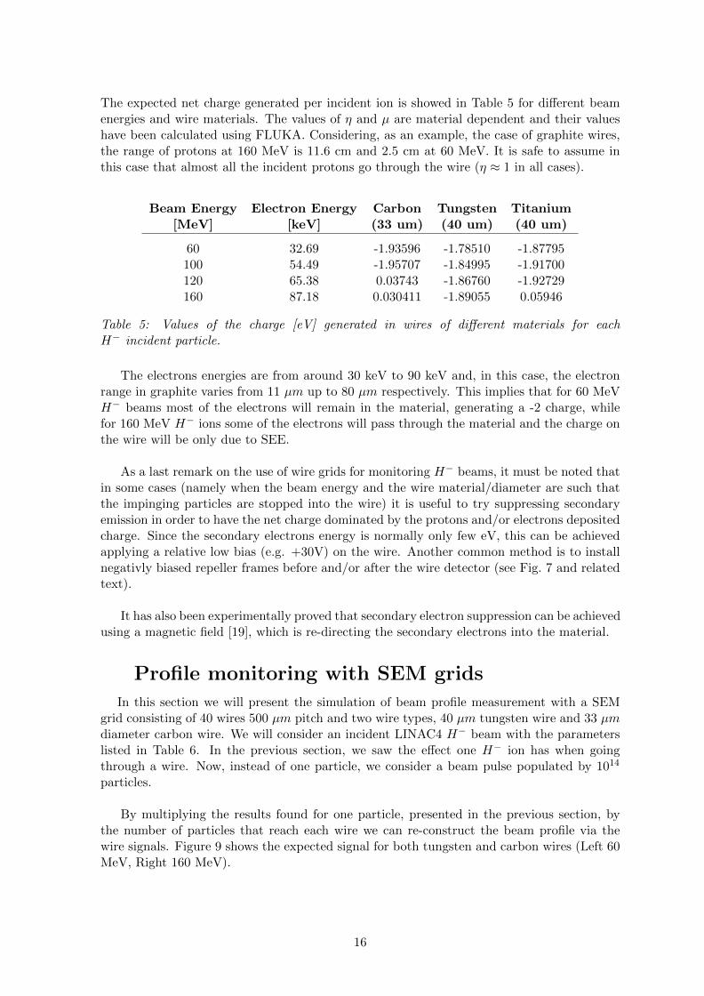
The expected net charge generated per incident ion is showed in Table 5 for different beamenergies and wire materials. The values of η and µ are material dependent and their valueshave been calculated using FLUKA. Considering, as an example, the case of graphite wires,the range of protons at 160 MeV is 11.6 cm and 2.5 cm at 60 MeV. It is safe to assume inthis case that almost all the incident protons go through the wire (η ≈ 1 in all cases).

Beam Energy[MeV]

Electron Energy[keV]

Carbon(33 um)

Tungsten(40 um)

Titanium(40 um)

60 32.69 -1.93596 -1.78510 -1.87795100 54.49 -1.95707 -1.84995 -1.91700120 65.38 0.03743 -1.86760 -1.92729160 87.18 0.030411 -1.89055 0.05946

Table 5: Values of the charge [eV] generated in wires of different materials for eachH− incident particle.

The electrons energies are from around 30 keV to 90 keV and, in this case, the electronrange in graphite varies from 11 µm up to 80 µm respectively. This implies that for 60 MeVH− beams most of the electrons will remain in the material, generating a -2 charge, whilefor 160 MeV H− ions some of the electrons will pass through the material and the charge onthe wire will be only due to SEE.

As a last remark on the use of wire grids for monitoring H− beams, it must be noted thatin some cases (namely when the beam energy and the wire material/diameter are such thatthe impinging particles are stopped into the wire) it is useful to try suppressing secondaryemission in order to have the net charge dominated by the protons and/or electrons depositedcharge. Since the secondary electrons energy is normally only few eV, this can be achievedapplying a relative low bias (e.g. +30V) on the wire. Another common method is to installnegativly biased repeller frames before and/or after the wire detector (see Fig. 7 and relatedtext).

It has also been experimentally proved that secondary electron suppression can be achievedusing a magnetic field [19], which is re-directing the secondary electrons into the material.

Profile monitoring with SEM grids

In this section we will present the simulation of beam profile measurement with a SEMgrid consisting of 40 wires 500 µm pitch and two wire types, 40 µm tungsten wire and 33 µmdiameter carbon wire. We will consider an incident LINAC4 H− beam with the parameterslisted in Table 6. In the previous section, we saw the effect one H− ion has when goingthrough a wire. Now, instead of one particle, we consider a beam pulse populated by 1014

particles.

By multiplying the results found for one particle, presented in the previous section, bythe number of particles that reach each wire we can re-construct the beam profile via thewire signals. Figure 9 shows the expected signal for both tungsten and carbon wires (Left 60MeV, Right 160 MeV).

16

Parameter Value Units

Top Beam energy 160 MeVBeam Pulse length 400 usRepetition rate 1.2 HzAverage pulse current 40 mASigma x * 2 mmSigma y * 1 mmAngular dispersion 0.49 mrad

Table 6: Main LINAC4 beam parameters. *These two values have been selected for thepurpose of this example

For 60 MeV H− ions we can see that the signal produced by a carbon wire, in absolutevalue, is bigger than the signal on the tungsten wire. In both cases the H− electrons aredeposited on the wire and SEE occurs. In the case of tungsten more secondary emission isexpected and therefore the positive charge left behind due to this phenomenon is expectedto be bigger than in the case of carbon.On the other hand, for 160 MeV the signal in carbon wires is positive because most of theH− electrons are able to exit the material. That leads to a positive signal which in absolutevalue is smaller than the one in the tungsten wire, which is still generated mainly by theincident H− electrons.

Figure 9: Expected current for Tungsten and Graphite SEM grids. Left, 60 MeV incidentH− ions. Right, 160 MeV incident H− ions. Both cases calculated with the parameters ofTable 6.

17

Emittance growth due to SEM

The aforementioned detectors are intercepting devices which means that have an effect onthe beam. As already discussed in Chapter 2, each time a particle traverses the detector’smaterial, it experiences Multiple Coulomb Scattering. Considering the particle ensamble, thisresults in an emittance increase at the monitor exit and, in case of large scattering angles,to beam losses. Such an effect is well know in literature, here we just present the result ofFLUKA simulations characterizing the scattering angle.

As an example, we considered a SEM grid which consists of 11 tungsten wires of 40 µmdiameter spaced 500µm, used to monitor a beam with initial σx = 2 mm and σy = 1 mm.FLUKA does not include the possibility of easily simulating H− ions so we have studiedindependently the effects of the detector on electrons and protons.

Figure 10: Histogram of protons’ angular distribution with respect to the beam direction 10cm after a SEM grid (11 tungsten wires, 40 µm thick, 500 µm pitch). Red line being theGaussian fit of the angular distribution. For 60 MeV protons.

Figure 11: Histogram of protons’ angular distribution with respect to the beam direction 10cm after a SEM grid (11 tungsten wires, 40 µm thick, 500 µm pitch). Red line being theGaussian fit of the angular distribution. For 160 MeV protons.

18

Figure 10 and 11 are a representation of the angular distribution with respect to thebeam direction 10 cm after the SEM grid. We can clearly observe how the angular spreadis bigger for 60 MeV protons (10) than for 160 MeV protons (11). This is not surprisingas the probability of interactions for low energetic particles is higher than the one for highenergetic particles. In this range of energies the electrons of an H− ion would be stopped inthe tungsten wires, so an study of the scattering angle is not easy in this case. If we considermore energetic ions it’s observed that changes in electrons’ trajectories are more drastic thanchanges in protons’ trajectories.

19

Chapter 4

Study of the beam induced wire heating

During the operation of the intercepting devices as wire grids and scanners, the energydeposited by the beam into the wire material translated into a temperature increase. Thiscan generate the loss of electrons by thermionic emission (thus affecting the wire signal) andpermanently damage the wires. Accounting for the various cooling mechanisms occurringduring and after the beam passage, this results in thermal cycles that are important to ad-dress in order to design the detectors and set limits for their operation.

In other words, the selection of the wire material and the the beam range of work (beamsize, intensity, duration) are limited, by thermal reasons. A good understanding of thevariation of the temperature and its consequences is therefore necessary [20]. The wirethermal behavior can be written as:

∆TTotal = ∆THeating −∆TRadadiative + ∆TThermoionic + ∆TConductive (19)

The beam pulse causes the temperature increase in the material of the detector andit is followed by three cooling effects, radiative cooling, thermionic cooling and conductioncooling. The equations used to describe these effects are nonlinear due to the dependence ofthe specific heat with temperature and due to the nature thermionic cooling. As a result, inorder to follow the thermal evolution, such equations have to be solved numerically.

Wire Heating

Given a beam pulse populated with NTot paritcles distributed in the horizontal and verticalcoordinates according to a Gaussian shape of width σxσy, the temperature variations of amaterial sample with surface ∆S and volume ∆V can be written as:

∆THeating =Ni

∆V · Cp (T ) · ρ· dEdx

(20)

where Cp(T) is the specific heat capacity of the material, ρ is the density, dE/dx the

stopping power of the particles in the material in units of[

Jm2g

]and

Ni = ∆S · NTot

2π · σx · σy· e

(− 1

2·((

xσx

)2+(yσy

)2))

(21)

refers to the fraction of NTot particles hitting the volume ∆V .

Radiative Cooling

In first approximation black body radiation is the dominant cooling effect and it is de-scribed by Stephan Boltzmann’s law. The heat radiated from the material surface is pro-portional to the forth power of the temperature and it is differentiated with the black bodyradiation by a factor called emissivity ε, that in most cases depend on the temperature.Discretized to our interests the model can be represented as:

20

∆TRadiative =∆S · σSB · ε (T ) ·

(T 4 − T 4

0

)Cp (T ) ·∆V · ρ

·∆t (22)

where, in addition to the variables defined above, ε (T ) is the emissivity, and σSB Stefan-Boltzmann’s constant (5.6704 · 10−8

[J/sm2K4

]).

Figure 12: Left, maximum temperature evolution on a carbon wire for a SEM grid. Right,maximum temperature evolution on a Tungsten wire for a wire scanner at three differentvelocities. All cases for a 3 MeV, 40 mA, 100 us pulse.

Thermoionic Cooling

With the increase of temperature, thermal energy is transferred to the electrons of thematerial. When the energy transferred to the charge carriers overcomes the work functionthey escape the material, leaving a charge equal in magnitude and opposite in sign. Thecurrent density emitted by the material is described by Richardson-Dushman [21]:

Jth = A · T 2 · e−φ(T )KT (23)

where φ is the binding potential (or work function) and A is Richardson’s constant,theoretically equal to:

A =4πmek

2qeh3

≈ 1.20173

[A

m2K2

](24)

with me the electron mass, k Boltzmann’s constant, qe the electron charge and h Plank’sconstant. This effect, called Thermionic emission, thus generates a net positive charge thatadds to SEE. In order to see how this effect can affect our SEE measurements, the thermioniccurrent for different materials and temperatures was calculated as shown in Table 7). In mostof the cases the estimated maximum temperature is below 1500 K and thermionic emission

21

Temperature Carbon Tungsten Titanium Alumina

300 0 0 0 01000 0 0 0 2.24e-141700 1.99e-9 1.59e-9 4.21e-9 4.64e-82600 1.94e-4 1.54e-4 2.73e-4 4.02e-33100 7.02e-3 5.62e-3 8.76e-3 1.38e-23500 6.14e-2 4.91e-2 7.11e-2 1.08e-14000 5.17e-1 4.14e-1 5.59e-1 8.31e-1

Table 7: Current due to Thermoionic emission in several materials. The numbers in redcorrespond to cases where the material is already melted. Melting points being 3773 K, 3695K, 1941 K and 2345 K for Carbon, Tungsten, Titanium and Alumina respectively.

can be neglected. Above this temperature the current density increases quickly but thecurrent due to secondary emission is still several orders of magnitude higher (for Tungstenwith a LINAC4 beam it was around 1 mA). For temperatures of the order of 2500-3000 Kthe thermionic emission and SEE magnitudes become comparable. Since these temperaturelevels are dangerously close to the material melting point, both Tungsten and Carbon wiresare not suitable for such high beam powers and thermionic emission will not be consideredin the signal calculations discussed later.

On the other hand, we will consider the material cooling due to the thermionic emission,which can be expressed as:

∆TThermionic = ∆S · (φ+ 2σBT ) · JthCp (T ) ·∆V · ρ

·∆t (25)

Thermal Conduction

Due to microscopic collisions of particles and movement of electrons within a body, heatflows from hotter to colder parts of the material. In our case the part of the materialthat is heated by the beam core reaches a higher temperature than the rest of the materialand therefore thermal conduction helps reducing the temperature in the hottest spots bytransferring the heat to the colder ones. This phenomenon can be described by the Fourierformulation detailed in [20]. Nevertheless, the contribution of conduction in the coolingeffects is very small compared with the radiative cooling. Because of this small contributionand the considerable increase on the simulation time, all the examples presented in thisdocument do not consider conduction effects as a cooling effect.

22

Temperature simulations

To estimate the heating and cooling of the detectors we assumed that the energy depositionis constant in the direction of the beam propagation. This approximation is not accurate forcases in which the Bragg peak occurs within the material thickness, because of low particleenergy and/or particular dense (or thick) materials. On the other end, the approximationholds for the cases considered below.

Table 8 shows the maximum temperatures reached in SEM grid detectors due to severalincident beam types. The results show that materials with higher density are not well suitedfor some beam characteristics. Gold has a relatively low melting point (1437 K), which isreached in the first two cases. The rest of the materials do not reach their melting pointtemperature but Titanium and Tungsten are close to it in the second case. Even thoughGraphite has a lower SEY compared with the rest of the materials, its thermal propertiesmake it one of the most common materials for this type of detectors. As we can see inFig. 12 right and Fig. 13, the equilibrium is reached after few pulses. Obviously, this kindof calculations are of primary importance at the moment of designing and specifying thefunctional specifications of a wire detector, which must feature an equilibrium temperaturesafely lower than any damage threshold.

Protons 60 MeV, I = 40 mA, Pulse length = 400 µs

Material TmaxBragg peak depth

[cm]Energy Deposition[

MeV cm2/g] Density[

gcm−3]

Graphite 755 2.03 9.642 1.7Titanium 956 0.94 7.510 5.506

Gold 2051 0.35 5.185 19.30Tungsten 2155 0.35 5.275 19.35




MeV cm2/g] Density[

gcm−3]


Gold 3943 0.35 5.185 19.30Tungsten 3374 0.35 5.275 19.35




MeV cm2/g] Density[

gcm−3]


Gold 1379 1.85 2.657 19.30Tungsten 1567 1.85 2.706 19.35

Table 8: Maximum temperature reached by SEM grids of different materials and for differentbeam types. Energy deposition and Bragg peak depth calculated using PSTAR

Even though we only discussed thermal issues, there are other processes that can lead toa wire damage, such as brittle failure, plastic failure or thermal fatigue. More details can befound in [22].

23

Figure 13: Temperature evolution of a tungsten wire due to 160 MeV proton beam, 100 µs

24

Chapter 5

Transverse beam emittance and slit-gridsystem measurement

This chapter contains a short introduction to the motion of particles in an acceleratorand the concept of emittance. Then, it will present the slit and grid emittance measurementtechnique, focusing on the system used for the LINAC4 LEBT emittance characterization.The chapter ends with the review of measurements performed during this thesis work andwill give some ideas for improving the monitor accuracy.

Basics of Beam Dynamics and Phase Space

The scope of the accelerator design is to guide the beam of particles along a referencepath and accelerate it into the desired energy. Charged particles are accelerated and focusedby magnetic and electrical fields. The reference system used to describe the movement ofthe particles is represented in Fig. 14. S defines the longitudinal coordinate and is alwaystangent to the reference path. X and Y define the transverse plane (orthogonal to the particletrajectory). x(s) and y(s) describe the particle’s deviations from the reference path at eachpoint, being x(s) = 0 and y(s) = 0 the reference path. Locally, the reference orbit has acurvature radius ρ (s).

Figure 14: Coordinates system used in beam dynamics

For the purpose of this document we are going to assume that the longitudinal and trans-verse planes are not coupled, i.e. the motion of the horizontal plane is not affected by theone in the vertical plane and the other way round. The reference orbit is a possible particletrajectory, particles with a nominal momentum p0 that start at some point with zero dis-placement will move along the designed orbit. In an accelerator facility the particle motion inthe machine is usually disturbed by field errors. In addition, we do not have single particlesbut particles ensembles in which each particle moves in a slightly different direction but the

25

center of gravity moves following the ideal orbit.

The principal elements of particle accelerators are those that provide the beam acceler-ation, guidance and focusing. The particles are accelerated by longitudinal electrical fieldsand the bending and focusing is provided by magnetic fields. The equation of motion of eachof those particles can be derived from Lorentz’s law and leads to the following expressionsfor the two transverse planes:

x′′ +

[1

ρ (s)2+

1

(Bρ)

∂By (s)

∂x

]x = 0 (26)

y′′ +1

(Bρ)

∂By (s)

∂xy = 0 (27)

where Bρ is equal to the ratio of momentum to charge, also called magnetic rigidity. Thedetailed solution of those equations can be found in [23]. Each particle is going to have at eachinstant of time a position and momentum. The x, y space only contains spatial informationof the particle distribution in a beam and merges both x(s) and y(s) in a single chart, seeFig. 15 left. Neglecting mutual interactions and coupling between the three coordinates wecan define the phase space of each degree of freedom of the system (see Fig. 15 right). Thephase space contains the whole description of the particles ensemble state for that particularplane.This information is required for calculating the subsequent motion of the particles inthe electromagnetic fields of the accelerator.

Figure 15: Left, example of x,y space. Right, example of phase space. Both images are purelyillustratives

The transverse beam emittances εx, εy are usually defined as the area (optionally dividedby π) of the phase space ellipse containing 95 % of all the particles. In a transfer line or ina storage ring (i.e. no acceleration) and assuming no energy losses due to radiation, eventhough the shape of the emittance ellipse can change, Liouville’s theorem establishes that theemittance is conserved [24]. In linear or circular accelerators (i.e. for particles experiencingenergy change) the emittance is not invariant but we can define the so called normalizedemmitance:

εN = βγε (28)

26

Where ε is quoted as geometric emittance and εN is the normalized emittance, which isconserved during acceleration.

Emittance measurement with a Slit-Grid system

For low energy linear accelerators, a typical method for measuring the transverse emit-tance consists in a slit-grid system, as schematically shown in Fig. 16. The system consistsin a movable slit with a small aperture that moves perpendicular to the beam direction. TheSEM grid is placed at a distance L. For each slit position the narrow aperture allows the pas-sage of a beamlet populated by particles that have almost an equal position x and a certainangular distribution. Thanks to the relative intensity read in each wire we are able to knowthe angular distribution of the particles at each grid position (X). Therefore, by scanning heslit across the beam the whole phase-space can be reconstructed.

In order to sample both transverse planes two slits and two grids are needed. The angularresolution of the monitor is determined by the profile monitor resolution (wire separation)and the drift space between the slit and the SEM grid. The geometry and material alsoeffects the measurement accuracy [25].

Figure 16: Schematic representation of a slit grid system

Emittance measuremets at 3MeV Test Stand

In order to obtain a stable source for LINAC4 , systematic simulations of hydrogen plasma andbeam formation are ongoing. Accurate measurements of the source emittance were needed tocheck the reliability of these simulations and the behavior of two different geometries of theplasma chamber extraction. The following pages will discuss the emittance measurements inthe 3 MeV Test Stand, the possible sources of uncertainty and propose some improvements.No further details about the source are given. If the reader is interested, more details aboutLINAC4 ’s source can be found in [26].

As mentioned in Chapter 1, between the source exit and the entrance of the first ac-celerator element, a Low Energy Beam Transport (LEBT) is needed to match the beam tothe RFQ requirements. The LEBT is equipped with diagnostics devices to control the beamquality and to supervise the performance of the source. The following measurements were

27

taken in the 3 MeV Test Stand which consists in a LEBT whose layout is similar to the oneinstalled in LINAC4 . A picture of the emittance meter installed in the 3MeV test Stand isshown in Fig. 17.

Figure 17: Scheme of 3 MeV Test Stand Emittance Meter

The system consists in two SEM grids and a stainless steel blade inclined 45 degrees rela-tive to the vertical axis. The blade is 1 mm thick and two 100 µm gaps have been machined,one parallel to the horizontal axis and the other parallel to the vertical axis. The SEM gridsare positioned 20 cm downstream the slit and consist of 40 Tungsten wires of 40µm of di-ameter, separated by 0.75 mm. Both the blade and the SEM grid are moved using steppingmotors and are mounted in 2 separate vacuum chambers. For each slit position, the corre-sponding grid can be moved with steps of 50µm in order to improve the overall resolution.

As a first approach some measurements of the beam emittance for different initial condi-tions were done. In these measurements we did a fast scan, that is, for each slit position theSEM grid stayed still. In this way the measurement time was reduced considerably but themeasurement angular resolution was limited. The motion of the emittance meter are limited,±35 mm for the slit, and ±70 mm for the SEM grid, defining a spatial scan range of ±35 mm.For each slit position the electronics is digitizing the each wire signal with a sampling periodof 4µs. By scanning the slit over all 75 mm, the phase space can be reconstructed (see Fig. 18).

After this first check of the system and of the beam emittance with a coarse scan, moreaccurate measurements imply displacing the grid in small steps for each slit position (toovercome the wire distance limitation). In addition, one has to properly setup the controland acquisition systems (e.g. wire signal gain) and be aware of possible misinterpretation ofthe results. In the following we will focus on the interpretation of the various SE sources andtheir effect on emittance measurement accuracy.

28

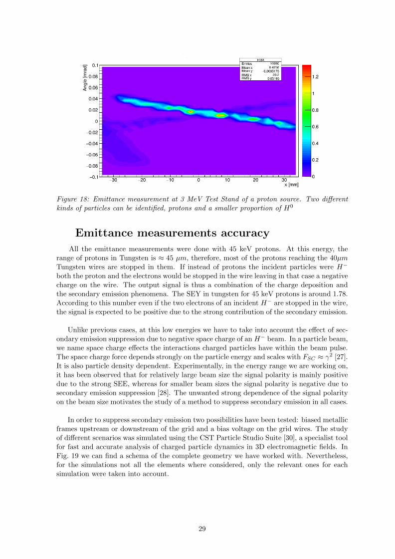
Figure 18: Emittance measurement at 3 MeV Test Stand of a proton source. Two differentkinds of particles can be identified, protons and a smaller proportion of H0

Emittance measurements accuracy

All the emittance measurements were done with 45 keV protons. At this energy, therange of protons in Tungsten is ≈ 45 µm, therefore, most of the protons reaching the 40µmTungsten wires are stopped in them. If instead of protons the incident particles were H−

both the proton and the electrons would be stopped in the wire leaving in that case a negativecharge on the wire. The output signal is thus a combination of the charge deposition andthe secondary emission phenomena. The SEY in tungsten for 45 keV protons is around 1.78.According to this number even if the two electrons of an incident H− are stopped in the wire,the signal is expected to be positive due to the strong contribution of the secondary emission.

Unlike previous cases, at this low energies we have to take into account the effect of sec-ondary emission suppression due to negative space charge of an H− beam. In a particle beam,we name space charge effects the interactions charged particles have within the beam pulse.The space charge force depends strongly on the particle energy and scales with FSC ≈ γ2 [27].It is also particle density dependent. Experimentally, in the energy range we are working on,it has been observed that for relatively large beam size the signal polarity is mainly positivedue to the strong SEE, whereas for smaller beam sizes the signal polarity is negative due tosecondary emission suppression [28]. The unwanted strong dependence of the signal polarityon the beam size motivates the study of a method to suppress secondary emission in all cases.

In order to suppress secondary emission two possibilities have been tested: biased metallicframes upstream or downstream of the grid and a bias voltage on the grid wires. The studyof different scenarios was simulated using the CST Particle Studio Suite [30], a specialist toolfor fast and accurate analysis of charged particle dynamics in 3D electromagnetic fields. InFig. 19 we can find a schema of the complete geometry we have worked with. Nevertheless,for the simulations not all the elements where considered, only the relevant ones for eachsimulation were taken into account.

29

Figure 19: Scheme of the geometry used. Blue: SEM grid Orange: polarization ring 1.Yellow, polarization ring 2

Lets begin with the suppression of secondary electrons using two polarized rings. In thiscase we are trying to suppress the secondary emission produced on the incident and exitingfaces on the wire. In order to simulate secondary electron production we considered thewires to be constant source of electrons. A typical beam size would be around 2 mm, thatis σx = σy = 2mm. The SEM grid is made of 40µm tungsten wires with a separation of500µm between each other. This tells us that the most affected wires are going to be the7 central wires. Therefore, we considered this seven wires as a source of 10eV ±10eV electrons.

Secondary electrons are negative charges therefore if we bias the rings with a negativevoltage, the electrons will be repelled and thus go back inside the wires. Furthermore, if thesecond ring is polarized with a bigger potential (in absolute value) than the first ring, anelectric field between them is going to be generated, making the electrons accelerate back tothe wire. This electric field can be made bigger if the first ring is biased with a positive signal(e.g. +1200 and -1200 V), but in that case the positive ring could attract some undesirednegative charges. Several configurations were tested, finally the polarization Ring 1 = -600V and Ring2 = -1200 V was selected, See Fig. 20.

The reason why we are trying to suppress SE with this two polarized rings is becausethey are currently installed in the LEBT. In reality these rings are placed downstream thebeam direction at a distance of around 63 mm from the SEM grid and their purpose was tosuppress the secondary electrons coming from a Faraday cup. Previously this Faraday cupwas placed 8 cm downstream the SEM grid affecting considerably the SEM grid measure-ments [31]. Currently this Faraday cup is palaced ≈ 1m downstream the SEM grid so SEemitted from the cup are not able to reach the SEM grid and affect its measurements. Atthe moment these rings are no longer useful for this purpose and as they are already installedthey could be used to cover other problems. Although the rings are placed downstream theSEM grid, in our simulations we’ve considered them to be before the SEM grid in order tosuppress the secondary electrons generated on the incident surface.

30

Figure 20: CST Particle Studio simulation of the effect of polarized rings on secondary emis-sion surpression. Left, no polarization on the rings. Right, Ring 1 = -600 V, Ring 2: -1200V

Now lets go back to our second objective, that is, trying to suppress secondary electronsemitted at angles around 90 and 270 degrees with respect to the angle of the particle’sincidence. These electrons are going to collaborate with the SE problem and also generatesome cross talk with the neighbor wires [32]. In this case both positive and negative biascan be used to suppress SEE. If we use a positive bias in a wire we are actually increasingthe work function and making it harder for secondary electrons to escape from the material.The problem with this method is that wires can also attract some undesired backgroundelectrons. The other option is to use negative bias in nonconsecutive wires. That allows usto repel background electrons and at the same time surprises secondary emission on the nonpolarized wire.

Figure 21: CST Particle Studio simulation of the effect of secondary emission supressionwith polarized wires. In this case the wires on the extremes are polarized at -10 V. The scaleis aplicable in all the previous cases.

31

In Fig. 21 we can see an example of 40µm Tungsten wires with the central wire as anelectron source and the neighboring wires polarized at -10 V. The main problem with thismethod is that negative polarized wires cannot be used afterwards as a source of informationto reconstruct the beam profile, so the accuracy of the measurement is affected. It is neces-sary to mention that all the results aforementioned have not been experimentally tested yet,they are only simulation results. So before concluding in their possible utility, further testsare necessary.

32

Chapter 6

LINAC4 ’s H0H− Monitors

At the moment, Linac2 is the first in the proton acceleration chain. The protons are acceler-ated form the few keV source to the 50 MeV LINAC2 top energy. As already discussed above,the LINAC2 will be replaced in 2019 by the new LINAC4 , which will bring H− particles upto 160 MeV. The injection into the PSB (4 rings, one on top of each other) will be performedby means of a H− charge exchange injection system, through a Carbon stripping foil (oneper ring), converting ≈ 99% of the beam to protons. In this chapter we will talk about thecharge exchange injection, what a stripping foil is and we will explain the arrangement ofthe H0/H− dump in the injection system. The core part of the chapter will focus on thenew H0/H− monitors, their setup and the detailed explanation of their calibration procedure.

Charge exchange injection (CEI)

Among other upgrades, it is foreseen to increase the LHC luminosity by providing thecollider with more bright (high density) beams form the injectors. At the moment, the firstof the brightness limitations is represented by space charge effects in the PSB, which will bestrongly reduced increasing the PSB injection energy from 50 MeV to 160 MeV. A furtherbrightness improvement is expected from the charge exchange injection (CEI) [33]. The pro-cess consists in the stripping of electrons from H− ions, followed by the capture of the newgenerated protons by the circular accelerator. Having the injected and circulating beam withopposite charge polarity, will allow increasing the density of particles in the beam.

The 160 MeV H− beam from the LINAC4 needs to be distributed to the 4 superposedsynchrotron rings of the PSB. After the beam is deflected to the four appropriate apertures,it will be injected into the PSB by means of an CEI system. Figure 22 shows the layout of

Figure 22: LINAC4 PSBooster injection Layout

33

the injection system. At each ring a set of 4 dipole magnets (BSW) will create the requiredinjection bump and a stripping foil will convert the H− beam to H+. Four internal H0 H−

beam dumps will be installed downstream each stripping foil in order to absorb any residualpartially stripped H0 and unstripped H− .

As already mentioned, the fundamental adventage of this technique is that due to theopposite charge of the injected and circulating beams the CEI can be designed for injectionof succesive turns into the same phase space, increasing in this way the brightness of thebeam [34].

Stripping Foil

In between the two BSWs we can find a foil. This foil is in charge of stripping the elec-trons from the H− ions, thus generating the protons to be injected into the PSB. Commonly,Carbon stripping foils are used. Carbon foils have the advantage of being the material withthe lowest Z that can be fabricated into a very thin foil, it is stable in vacuum at high tem-peratures and has good electrical and thermal properties [35].

After the H− beam goes through the stripping foil we can find three types of particlesremaining, H+ (protons), if two electrons were stripped, H0 if only one electron was strippedand H− if neither of the electrons were stripped. There could also remain other types ofparticles due to the possibility of electron pick up. However, for energies above 100 keV thecross sections for electron pick up can be neglected. The ratio of H+ after the stripping foilis given by [36]:

fH+ = 1− 1

σ−1,0 + σ−1,1 − σ0,1

[σ−1,0e

−σ0,1x − (σ0,1 − σ−1,1) e−(σ−1,0+σ−1,1)x]

(29)

where σ−10, σ01, σ−11 are the cross sections of the reactions H− → H0+e−, H0 → H++e−

and H− → H+ + e− + e−, respectively. x = N0τ/A, where A is the atomic number of theCarbon foil and τ is the area density. The stripping inefficiency can be expressed as:

fH− = e−σ−1,0x (30)

Therefore, the yielding of H0 can be expressed as:

fH0 = 1− fH+ − fH− (31)

Table 9 shows a summary of the cross sections at different energies. For a given foil thick-ness the stripping efficiency is higher if the energy is lower. Also, a relation between strippedelectrons and foil thickness can be found. The proportion of H+ and therefore the proportionof stripped electrons increases as the foil thickness increases, whereas the proportion of H0

has a maximum for a given thickness. The proportion of H− decreases with the foil thickness.

Even if the efficiency is bigger for smaller energies and thicker foils, we have to pay at-tention to the temperature evolution of the foil and the effect it has on the beam emittance.In the charge exchange injection, both H+ and H− cross the foil and deposits energy on it.The thicker the foil and the lower the energy, the greater the energy deposition and the beam

34

80 MeV 250 MeV

σ−1,0 3.17 1.35σ0,1 1.24 0.53σ−1,1 0.056 0.024

Table 9: Cross sections of the reactions H− → H0 + e−, H0 → H+ + e− and H− →H+ + e− + e−. Units 10−18cm2 . From [36]

emittance blow up.

In the case of LINAC4 , several foil types are being tested. The foil will need to beabout 20 mm high and 20 mm wide, with a thickness between 100 and 200 µm/cm2. Duringinjection, it is expected to find a current of H0 around 2% of the LINAC4 beam pulse currentcorresponding to an stripping efficiency of 98%. The level of H− coming from the strippingfoil would be even lower, around 10−6%, although the current of H− can be higher becauseof the halo particles of the beam that miss the stripping foil.

H0H− Monitors in PSB HST

As discussed above, the future injection of LINAC4 ’s beam into the PSB will be basedon the CEI technique. The PSB comprises 4 rings and one of this injection structures willbe installed in each ring. The magnetic field of the BSWs is such that the protons reachthe circulating beam, see Fig. 22. H0 and H− are not going to be affected by the magneticfield on the same way as protons. H0 are neutral and will not be affected, whereas H−

are going to be bent in the opposite direction. These unwanted H0/H− particles will bestopped by a dump, see Fig. 23. H0/H− monitors will be installed in front of each dump inorder to monitor the stripping efficiendy and so to assure a good injection. The system wastested for the first time in the PSB Half Sector Test (HST) where all the measurements ex-plained in the following sections were taken. Other measurements results can be found in [37].

Figure 23: Mechanical representation of the H0H− dump and monitors on the beam pipe.

These H0H− monitors consists in two Titanium plates of 1 mm of thickness. Each plateis divided in two halves with a cut placed on the center. This additional feature adds beamposition information to the intensity measurements. The monitors were placed inside theBSW4’s magnetic field at a distance of 4 cm from the dump’s face. This distance is enough

35

to avoid the secondary electrons coming from the dump to affect the monitors’ signal. Thesemonitors are connected to an interlock circuit, that is, if the intensity measured surpassesa safety limit, now set to 10% of the LINAC4 ’s peack intensity, the interlock circuit willstop the beam. So far this feature is not yet implemented as the monitors are still beingtested. Before reaching that point, the monitors and the electronics behind them have to becalibrated and cover all their required features.

Figure 24: Production drawing of the H0H− plates with dimensions and tolerances.

During normal operation, the current in the H0 plates is expected to be up to 2% ofthe nominal LINAC4 ’s current, which corresponds to around 0.5mA. Stripping degradationcan be tolerated until 10% of the nominal intensity which would correspond to a signal of≈ 4mA. This should be the threshold at which the interlock circuit stops the beam. In avery first approximation the expected signal per impinging H− would be 2 electron chargesand 1 electron charge for H0 plates. A more precise determination of the net charge left perincident particle can be found in Table 10.

BS SEY BS δH [e/H−] H

[e/H0

]w S.E w.o. SE w SE w.o SE

Titanium 0.23 0.0114 0.025 -1.42 -1.49 -0.61 -0.7336

Table 10: Expected net charges per impinging 160 MeVH0 andH− particle in 1mm Titaniumplate.

The electronics readout is designed for integrating the charge in each plate between 50ns and 1 µs. So the total number of charges read at each plate will depend on the beamintensity, beam pulse leangth and integration time. The injection time can vary between 50ns to 150 ns. The 50 ns lower limit has been specified to be consistent with the minimumdetectable signal.

36

Electronics conceptual design and available signals.

The electronics after the monitors are designed to ensure a continuous measurement ofthe H0H− particles, to function as an interlock system to protect the dump and thereforeto assure an efficient injection. Only a conceptual explanation is going to be given in thissection, for more detailed description the reader may check [18]. Several versions of the elec-tronics where tested during the measurements but all of them shared the same basic structure.

Figure 25: Schematic layout for the continuous monitoring system.

The system is divided in two main subsystems, the interlock circuit and the continuousmonitoring system. One of the requirements is that the signal does not saturate even in thecase of foil breakage. For this reason the continuous monitoring system has been split intotwo sub-circuits, high gain electronics and low gain electronics. With the high gain elec-tronics the pulse length can go down to 50 ns but requires a long time for discharging theintegrators. The low gain electronics allows the pulse to be longer than 70 ns, it includes twoalternating fast integrators connected to a fast ADC that converts the integrated charge intodigital samples spaced 1 µs. In this continuous monitoring circuit, shown in Fig. 25, alsoan unprocessed signal is at our disposal. This signal is connected to an oscilloscope channel(named OASIS) after passing through a fast amplifier. The interlock circuits on the board,see Fig. 26, comprises a slow and low gain amplifier fed with the outputs of each plate. Theintegrator will be connected to a comparator (or two consecutive comparators depending onthe version of the circuit) that has as a second input a predefined reference.

In the following sections we are going to talk about the analysis of the signals coming

37

from the OASIS scope, the ADC converter. Not a lot of details concerning the interlocksignal will be given.

Figure 26: Schematics of the interlock circuit.

Measurements procedure.

The main goal of these measurements was to obtain a calibration factor which, indepen-dently of the intensity or type of beam, was able to relate the signal on the plates with thenumber of particles reaching the dump. For that, several measurements with different beamlengths and intensities were taken. The procedure of the measurements was always the same.The beam was scanned along the four plates from left to right giving special attention to thepoints where the beam was between two plates and when it was at the center of one plate. Thesequence of the measurements was the one indicated in Fig. 27. In the following pages we willrefer to those points as H0L, H0LH0R, H0R, H0RHML, HML, HMLHMR, HMR respectively.

Figure 27: Schema of the order followed during the measurements.

In order to find the calibration factor the measurements were done with an H− beamimpinging directly to the plates rather than first going through the stripping foil. This ap-

38

proach was chosen in order to reach all the plates with a beam of the same characteristics. Ifthe beam goes through the stripping foil, the particles reaching the monitors are going to bemostly H0 , in a quantity dependent on the foil’s efficiency. At the same time, if the incidentparticles were H− it was possible to reach all the plates by choosing an appropriate magneticfield value for the BSW3 and BSW4 magnets. On the contrary, if the particles were H0 ,only the first two plates were reachable.

Oasis Signals and first conclusions

When referring to OASIS signals, we are actually referring to the analytical signals com-ing from the plates. Only a fast amplification is applied to these signals before going to thescope. Image 28 shows an example of the type of signal read out by the plates. Two differentprocedures were followed in order to analyze these signals. The first consisted in calculatingthe signal integral in time. This allow us to obtain the total number of charges detectedby the plate in one beam pulse. Afterwards, this value was normalized by the total numberof charges detected by the closest Beam Current Transformer (BCT). The second methodconsisted in calculating the mean value of the signal along the pulse and normalizing it by thecurrent measured by the BCT. Both types of analysis seemed to give pretty similar results.The integral method was finally chosen for practical reasons.

Figure 28: Example of OASIS scope traces of a 4 mA,5 µs H− beam. In this case the beamwas placed on the center of the HMR plate.

Figure 29 summarizes the response of the plates to different intensity beams. In thisparticular set of measurements, we were interested in understanding, qualitatively, how theplates responded to different beam intensities and also to see, if a different response was ap-preciated between the different plates. In order to appreciate this relative difference, Fig. 29is also normalized by the value of signal measured in H0L plate. From this graph we can seethe effect of the plate’s gaps (1 mm). In the majority of the measurements it is also evidentthat the H− plates provided a slightly higher signal than the H0 ones.

As mentioned in Chapter 2, it has been experimentally demonstrated that secondaryemission can be suppressed by using magnetic fields. In our scenario, we scan the beam alongthe plates thanks to BSW3 and BSW4’s magnetic fields. Particularly, for the beam to reach

39

Figure 29: OASIS measurements for different beam intensities. Beam scanned using bothBSW3 and BSW4. X axis, position of the beam at the moment of the data extraction. Yaxis, each point represents the sum of all the signals of the plates for that particular intensityand position normalized by the number of charges measured by an upstream BCT and alsodivided by the signal on the H0L plate.

H0R plate, no magnetic field was needed. In order to reach H0L a very small magnetic fieldwas necessary whereas if we wanted to reach the H− plates it had to be higher. In the platesthe signals are mostly negative due to the charge deposition of the incident H− ions. Due toSE, electrons are emitted from the surface making the signal to become less negative. If SE issuppressed by magnetic fields it would explain why signals on the H− plates are higher thanthe H0 plates’ signals. In order to check this theory, several measurements were done scanningthe beam only with BSW3 and keeping BSW4 to a constant value. The monitors are placedinside BSW4’s magnetic field so keeping BSW4 at a constant value of around 0.12 Tm wouldmake SE the same for all the measurements. Figure 30 shows the summary of these measure-ments. In this figure it is clearly appreciated how the signal difference between the H− andH0 plates is no longer existent, thus confirming the SE suppression by the BSW4 field theory.

Figure 30: OASIS measurements for different beam intensities. Beam scanned with BSW4’smagnetic field constant.

40

Digitized signals and calibration factor.

The procedure followed to analyze OASIS signals was also followed in order to analyzethe signal of the plates after the electronics. The effects of the holes and the tendency up forthe H− plates was, as expected, also observed with the digitized signals. In order to studythe response of all the plates under the same conditions, all the following measurements weretaken with BSW4’s magnetic field at a constant value. In this analysis we were interestednot only in a qualitative result but also in quantifying a calibration factor able to relate thesignal read out by the plates with the total number of particles reaching the dump. A linearbehavior with the intensity was expected. The higher the intensity the higher the read outsignal.

In Fig. 31 a summary of the digitalized signals is presented. Each point of the graph cor-responds to the signal read out of the respective plate normalized by the number of chargesdetected by the last upstream BCT. We can clearly differentiate two different families ofgroups. Group 1, points around 0.6 · 10−6. Group 2, points around 0.3 · 10−6. Each groupcorresponding at each one of the versions of the electronics that were tested during the mea-surements. Several uncertanities were observed with the latest version of the electronics(Group 2), so espetial attention will be given to the Group number 1.

Figure 31: Signal read out by the different plates and for different intensity values. Normalizedby BCT.1043’s intensity . Each color corresponds to each one of the plates. Two groups ofpoints are sighted, Group 1, points around 0.6 ·10−6, measurement done 3rd and 4th of April.Group 2, points around 0.3 ·10−6, measurement done 6th of April. Each group correspondingon a version of the electronics behind the detectors.

In Fig. 31, due to the normalization by the BCT’s measured charges, instead of obtainingan straight line with a constant slope, the points on the graph are distributed along this slopevalue. A more accurate approach to this slope value is shown in Fig. 32. On the top part ofthe image we can find an histogram of the different registered values, the mean value being6.807 · 10−7 . In Fig. 32 bottom, we can find the relative errors from the measurements withrespect to this mean value. Some variations are found between plates and beam intensities,but all the values are around 6.807 · 10−7 with a relative error smaller than ±2%.

41

Figure 32: Top, histogram of the callibration factor (Digital signal / BCT signal) for differentintensities and plates. Bottom, Relative error in % of the callibration factors for differentplates and intensities. Both graphs corresponding to the version of electronics tested the 3rdand 4th of April.

Reliability of k factor for H0 signals.

A second set of measurements was carried out while testing different stripping foils. Asin the previous measurements, several beam intensities were used. Figure 33 summarizes theresponse of the plates to different beam intensities while using hybrid Boron Carbon foils [38].In this graph only the case with BSE3 and BSW4 at nominal current (3092 A) is represented.From the image we can appreciate that in all the cases the signal is mainly on the H0R plate.A non negligible signal can also be found in the HMR plate. In order to certify which kind ofparticle was reaching each plate some of these measurements were also taken with a differentvalue of the BSWs’ current. The only difference found between the measurements was thesignal measured by the HMR plate. This means the signals on the H0L, H0R and HML platesare generated by H0 whereas the signal on the HMR plate is generated due to H− particles.

42

Once again, we can find two different families of measurements corresponding to the twodifferent models of the electronics tested. To be consistent with the calibration factor cal-culated on the previous section, the rest of the results will only include the data from thecorresponding version of the electronics (points around 0.8 · 10−9).

Figure 33: Signal read out by different plates normalized by number of charges measured withBCT.1043. Each color correspond to each one of the plates. Measurements taken using ahybrind Boron-Carbon Foil.

k = 6.807 · 10−7 was the value of the calibration factor found on the previous section.This value relates the signal coming from each plate, in ADC units, with the total number ofparticles reaching each plate. Using this value we can calculate the total number of incidentparticles. This value can be compared with the number of charges measured by the BCT be-fore the stripping foil. The ratio between these two values will give the stripping inefficiencyof the corresponding stripping foil. For doing those calculations, an important detail has tobe taken into account. k was calculated with an incident H− beam. In order to be able touse this calibration factor we have to take into account the differences on the signal producedby an H0 or an H− particle.

If we go back a couple of pages, Table 10 shows the relative difference between signalsdue to H0 and H− particles. This difference being 2.328 with secondary emission and 2.031without secondary emission. In our case a relative high magnetic field was present duringthe measurements so we can assume SEE was suppressed. If we want to use the k factorfor a signal produced by H0 particles, it should be divided by a factor 2.031 as the signalproduced by H− is twice the one produced by H0. Formula 32 summarizes how the strippinginefficiency is calculated using the signal measured by the plates and the calibration factor.

SI =1k · (2 ·ADCH0L + 2 ·ADCH0R + 2 ·ADCHML +ADCHMR)

#ChargesBCT.1043(32)

If we follow the procedure explained on the previous paragraphs we obtain a strippinginefficeincy of 0.234% for stripping foil 6 and 0.369% for stripping foil 5, see Table 11. An-other method to measure the stripping inefficiency is also available. Along these pages we’vebeen talking about BCT.1043 which allowed to measure the number of particles before the

43

stripping foil. Another BCT is placed downstream the stripping foil, that is BCT.1073. Di-viding the number of charges measured by the BCT downstream and the BCT upstreamthe stripping foil, we are able to calculate the stripping efficiency. On the previous case wecalculated a stripping efficiency of 98.61% for SF 5 and 98.75% for SF6, or what is the same,a stripping inefficiency of 1.389% for SF5 and 1.243% for SF6.

A non negligible difference appears when measuring the stripping inefficiency by thesetwo different methods. The reason for this discrepancy can be explained if we include in ouranalysis the possible lost of protons between the two BCTs. Let’s give this a little more ofcontext.

DescriptionFoil

NumberSize[mm]

XCF-200, arc evaporated amphous Carbon, collodion caoated 1-4 32 x 68DLC-23-1000-S, Diamond-like Carbon, boron doped 10% 2-3 32 x 68HBC, Hybrid type Boron mized Carbon 5-6 21 x 68

Table 11: Characteristics of the different foil types used. From [38]

6 different stripping foils were tested. In Table 11 we can find a summary of the character-istics of these different stripping foils. For the first 4 stripping foils no signal was appreciatedon the plates, or the signal was too small to clearly differentiate it from noise. Nevertheless,in those cases also a stripping inefficiency of ≈ 1% is measured by the BCTs. This could beexplained if some protons were lost before reaching the BCT downstream the stripping foil.If that was the case the missing particles could not be counted as stripping inefficiency asthey have been correctly stripped. If in all the cases we consider that 1% of the particles aregoing to be protons lost between the two BCTs, the stripping inefficiency calculated with theBCTs would be ≈ 0.389% for SF 5 and ≈ 0.243% for SF 6.

Figure 34: Distribution of the stripping inefficiency as measured by the H0H− monitor and bythe BCTs over about 700 LINAC4 pulses, with two different Hybrid Boron Carbon strippingfoils.

44

Figure 34 is a quantification of the previous explanation. The red and black lines cor-respond to the histograms of the stripping inefficiency calculated with the plates for SF 6and SF 5 respectively. Alike, the green and blue curves are the histograms of the strippinginefficiency calculated using the BCTs. All these histograms have been normalized by thetotal number of entries so measurements with both stripping foils can be compared.

All the results presented in this chapter where calculated using the signal from the contin-uous monitoring system. The interlock signal was also available. A clear linear dependencewith beam intensity was observed over a large intensity range [39]. Nevertheless, no furthertests were done to study in detail the interlock functionality.

The Half Sector Test stopped activities on the 6th of April 2017 after around 3 monthsof operation. This period was very useful to verify the performance of the H0H− beamcurrent monitors. Nevertheless, this period was not enough to fully establish the absoluteaccuracy of the device, study in detail the interlock functionality or test the final version ofthe electronics. Ways to complete these studies are now being investigated.

45

Conclusions

The first month of the work at CERN was dedicated to understand the particle interactionwith matter, with emphasis on Secondary Electron Emission phenomena. Afterwards it waspossible to learn how Secondary Emission Monitors (SEM) use this effect for transverse beammonitoring (Chapter 2). SEM comprehend an assortment of different types of detectors. Inthis thesis SEM grids and Wire Scanners are the ones presented with more detail even thougha bunch of other types of detectors also exist (Chapter 3).

Due to their intercepting nature, SEM detectors have an effect on the beam (emittanceblow up). At the same time the beam has an effect of them (Signal generation, thermalfluctuations, etc.). Several python routines were implemented in order to simulate, amongothers, the previous phenomena, that is, emittance growth, signal generation and tempera-ture evolution of the monitors (Chapter 4). If not indicated otherwise, the results presentedin this thesis have been calculated with the aforementioned routines. It is foreseen that userfriendly versions of these programs will be available after August 2017 if no other prioritiescome up.

Even if it was not with a lot of detail, softwares like Fluka and CST Particle studio werelearned and used. Some results calculated with these programs can be found along the pages.

Beam profile measurements where taken with SEM grids and Wire scanners although fi-nally these measurements where not included on this document. Neither emittance measure-ments (Chapter 5) nor H0H− calibration (Chapter 6) were included on the initial planningof the work. Nevertheless, the need for these measurements and its relevance were reasonsenough to include them.

Special attention should be given to references [37], [38] and [39]. These three articles werepublished during May 2017 for IPAC conference in Copenhagen, Denmark. Concretely, [37]includes general information about the Half Sector Test and the measurements performedsince it firstly received beam on October 2016. [38] presents detailed information about thestripping foil units tested in the HST as well as their operational experience. Finally, [39]includes a summary of the beam instrumentation available in LINAC4 and PSB HST as wellas a summary of the results presented in Chapter 6.

46

References

[1] L. Arnaudon, et al. Linac4 Technical Design Report. CARE-Note-6006-22-HIPPI, CERN,Switzerland.

[2] NIST, National Institute of Standars and Technology. Physical Meas. Laboratory.

[3] A. Missimiliano Schiavi, Study of Laser produced Plasmas by X-Ray and Proton Radiog-raphy, Plasma Physics Group, PhD, London,2003.

[4] D.E. Groom, et al., Muon Stopping Power and range Tables 10 MeV- 100TeV, AtomicData and Nuclear Data Tables, Vol 76., No, 2, July 2001.

[5] K. Nakamura et al. (PDG), Passage of particles through matter, February 16, 2012, JPG 37 075021.

[6] W. Frass,Passage of particles through matter, Oxford physics 2009.

[7] D. Krammer, Design and Implementation of a Detector for High Flux Mixed RadiationFields, Department of physics, University of Livec, Phd, Czech Republic, 2008.

[8] D. Hasselkamps, et al. Ion induced secondary electron spectra from clean metal surfaces,Nuc. Instrum. and Methods Phys. Res. B 18 (1987) 561.

[9] http://www.fluka.org/fluka.php

[10] G.Lakits, et al., Statistics of ion-induced electron emission from a clean metal surface,American Institute of physics, 22 June 1989.

[11] E. Borokovsky, et Al. The secondary-electron yield measured for 5-24 MeV protons onaluminium-oxide and gold targets, Nuclear Instr. and Methods in Physics Research, 1988.

[12] P.Thieberger, et al. Secondary-electron yield and their dependence on the angle of inci-dence on stainless-steel surfaces for three energetic beams, Physicak Review, Volume 61,04291

[13] http://www.cloudylabs.fr/wp/nombre-de-delta-ray/

[14] Allan J. et al. Backscattering and secondary electron emission from metal targets ofvarious thiknesses, Washinton, D.C., April 1965.

[15] V.L. Highland. Some practical remarks in multiple scattering, Nucl. instr. and meth,Vol.129 p.497, 1975.

[16] G.R. Lynch and O.I. Dahl. Approximation to multiple Coulom scattering, Nucl. instr.and meth, Vol. B58, p.6, 1990.

[17] U.Raich, Beam Diagnostics, CERN, Geneva, Switzerland.

[18] F.Roncarolo, et al. H− and H0 beam current monitor electronics., PSB-BC-ES-0001,CERN, Geneva, Switzerland.

[19] L.Wang, et al. , Suppression of secondary emission in a magnetc field using a swatoothand isosceles triangle surface, SLAC, Menlo Park, CA, USA.

47

[20] M. Sapinski, Model of Carbon Wire Heating in Accelerator Beam, CERN, Geneva,Switzerland, 2008.

[21] Gorazd Planinsic, Thermionic Emission,University of Ljubljana, Department of physics,April, 2008.

[22] M. Moser, Fractography with the SEM (Failure Analysis), 2007.

[23] F. Roncarolo, Accuracy of Transverse Emittance Measurements of the CERN LargeHadron Collider, Ecole Polytechnique federale de Lausanne, PhD Lausanne, 2005

[24] J. Buon, Beam Phase space and Emittance, LAL, 91405 Orsay, France

[25] F.Roncarolo, et al., Accuracy determination of the CERN LINAC4 emittance measure-ments at the test bench for 3 and 12 MeV. CERN Geneva Switzerland. 2010.

[26] J. Lettry, et al. , LINAC4 H* ion sources, Review of scientific instruments 87,02B139,2016.

[27] M. Lutz, CERN LINAC4 - The Space Charge Challenge, University of Berlin, PhD,2013.

[28] U. Raich, et al., Commisioning of the CERN LINAC4 wire scanner, wire grid and slit-grid monitors at 3 and 12 MeV, Proceedings of Linac, 2014, Geneva, Switzerland.

[29] B. Cheymol, et al., Scattering of H− Stripped Electrons from sem grids and wire scanersat CERN LINAC4 , Proceedings of LINAX2012, Tel-Aviv, Israel.

[30] https://www.cst.com/products/cstps

[31] B. Cheymol, et al. , Comissioning of the LINAC4 ion source transverse emittance meter,CERN-BE-2010-014 BI.

[32] F. Roncarolo, et al., Effect of H− stripped electrons on the LINAC4 profile measurements,CERN-ACC-NOTE-2014-008 TECH

[33] C.Hojvat, et al., The multiturn charge exchange injection system for the fermilab boosteraccelerator, IEE Transactions on Nuclear Science, Vol. NS-26, No 3, June 1979.

[34] T. Kawakubo, et al., The H− exchange injection system in the booster of the KEK 12GeV proton Synchrootron, National laboratory for high energy Physics, Japan.

[35] V. Lienchtenstein, Carbon Stripper Foils- Preparation and quality, Kurchatov Institute,123182 Moscow, Russia.

[36] Huang Ming-Yang, et al., The effects of injection beam parameters and foil scatteringfor CSNS/RCS, institute of high energy physics, China, 2012.

[37] B. Mikulec, et al. Commissioning and results of the half-sector test installation with 160MeV H− Beam from LINAC4 , CERN, Geneva Switzerland. .

[38] C. Bracco, et al. Commissioning of the stripping foil units for the upgrade of the PSBH− injection system, CERN, Geneva, Switzerland.

[39] F. Roncarolo, et al. ,Beam instrumentation for the CERN LINAC4 and PSB Half SectorTest, CERN, Geneva, Switzerland

48

Characterization and optimization of CERN Secondary ...

Documents

Transcript of Characterization and optimization of CERN Secondary ...