CHARACTERIZATION AND MODELING OF CREEP BEHAVIOR IN …

The Pennsylvania State University

The Graduate School

Department of Engineering Science and Mechanics

CHARACTERIZATION AND MODELING OF CREEP BEHAVIOR IN AMBIENT

TEMPERATURE CURED THERMOSET RESIN

A Thesis in

Engineering Mechanics

by

Anurag Jaipuriar

2011 Anurag Jaipuriar

Submitted in Partial Fulfillment

of the Requirements

for the Degree of

Master of Science

August 2011

ii

The thesis of Anurag Jaipuriar was reviewed and approved* by the following:

Charles E. Bakis

Distinguished Professor of Engineering Science and Mechanics

Thesis Advisor

Maria Lopez de Murphy

Associate Professor of Civil Engineering

Renata S. Engel

Professor of Engineering Science and Mechanics

Associate Dean for Academic Programs

Judith A. Todd

P.B. Breneman Department Head Chair

Professor of Engineering Science and Mechanics

*Signatures are on file in the Graduate School

iii

ABSTRACT

Externally bonding fiber reinforced polymer (FRP) composites to existing structures as a method

of increasing strength is a quick and convenient retrofitting technique for structurally deficient

structures. FRP strengthening systems typically utilize an ambient cured epoxy resin as matrix as

well as adhesive. Ambient cured epoxies may have a glass transition temperature (Tg) close to the

service temperature. The Tg being close to service temperature results in increased rate of

physical aging which in turn results in the evolution of material properties. At temperatures close

to Tg, creep deformation in the epoxy resin is also magnified. Hence it is important to characterize

the Tg and creep behavior in the constantly evolving ambient cured epoxy resin. Dynamic

mechanical analysis (DMA) and differential scanning calorimetry (DSC) were utilized to study

the Tg evolution with age of epoxy. For a 7-day-old epoxy the onset of glass transition was around

40°C. An increase in Tg of almost 15°C was observed between a 7-day-old resin specimen and a

specimen aged 100 days at room temperature, based on the dynamic storage modulus. The

differences in various methods of assigning Tg mechanical and thermal testing was also observed.

To gain understanding of the increase in Tg with material age, cure kinetics and physical aging

kinetics models for the epoxy resin were developed. Physical aging at ambient temperature was

identified as the reason for the increase in Tg of the resin. An “extent of aging” parameter was

proposed to parameterize the evolution of epoxy resin towards equilibrium at the aging

temperature. To characterize the creep response, tensile tests of plain epoxy coupons were done at

ages of 7, 30 and 100 days at three different temperatures—22°C, 30°C and 35°C. As the

specimen aged, it became stiffer and creep compliance and creep rate decreased dramatically for

given testing temperatures. The knowledge of physical aging kinetics was utilized to link the

mechanically observed creep behavior to “extent of aging” parameter. The novelty of this

technique is in the ease with which aging can be characterized for a complex thermal history of

polymer which governs its creep behavior. The advantage of using this technique over preceding

iv

work to model non-isothermal aging is that creep response is not derived from parameters of a

structural recovery model but a more tangible experimentally measured quantity. A MATLAB

based code was developed based on this technique to predict the creep behavior of resin aged at

22°C for a variable time and then subjected to creep loading at different temperatures. The

predictions of the analytical model were in good agreement with the experimentally observed

creep behavior for most of the cases, particularly in terms of creep rate at times greater than 50

hours.

.

v

TABLE OF CONTENTS LIST OF FIGURES……………………………………………………………...………………………….……………………vii

LIST OF TABLES……………………………………………………………………………………………………………………x

ACKNOWLEDGEMENTS……………...…………………………………………………..xi

Chapter 1 Introduction ............................................................................................................. 1

1.1 Externally Bonded FRP reinforcement ...................................................................... 1

1.2 Effect of Elevated Temperature and Sustained Loading ............................................ 4

1.3 Motivation and Research Objectives ......................................................................... 7

Chapter 2 Characterization of Glass Transition Temperature.................................................. 8

2.1 Introduction ................................................................................................................ 8

2.1.1 Assignment of Tg using DMA ................................................................................. 10

2.1.2 Assignment of Tg using DSC .................................................................................. 11

2.2 Experiments ............................................................................................................... 14

2.2.1 DMA Characterization of Tg ........................................................................... 14

2.2.2 DSC Characterization of Tg ............................................................................. 19

2.3 Results and Discussion ............................................................................................... 20

2.3.1 DMA Results ................................................................................................... 20

2.3.2 DSC Results .................................................................................................... 28

2.4 Conclusion ................................................................................................................. 30

Chapter 3 Investigation of Cure Kinetics and Physical Aging Kinetics in Epoxy Resin ......... 32

3.1 Introduction ................................................................................................................ 32

3.1.1 Literature Review on Cure Kinetics of Epoxy Resin ...................................... 32

3.1.2 Literature Review on Physical Aging Kinetics of Epoxy Resin ..................... 34

3.2 Experimental Program ............................................................................................... 40

3.2.1 Chemical Cure Kinetics .................................................................................. 40

3.2.2 Physical Aging Kinetics .................................................................................. 41

3.3 Results and Discussion ............................................................................................... 41

3.3.1 Model for Prediction of Degree of Cure (α) .................................................... 41

3.3.2 Physical Aging Evolution Model .................................................................... 48

Chapter 4 Prediction of Tensile Creep Behavior in Epoxy Resin ............................................ 53

4.1 Introduction ................................................................................................................ 53

4.2 Objectives................................................................................................................... 54

4.3 Literature Review ....................................................................................................... 54

4.4 Experiment ................................................................................................................. 62

4.4.1 Tensile Creep Test Specimen Preparation ....................................................... 62

4.4.2 Creep Test Set-up ............................................................................................ 63

4.3.3 Creep Test Program ......................................................................................... 66

4.4 Creep Test Results ..................................................................................................... 68

vi

4.5 Modeling Creep Response in Epoxy Resin ................................................................ 77

4.6 Conclusion ................................................................................................................. 91

Chapter 5 Conclusions and Recommendations for Future Work ............................................. 92

5.1 Conclusions ................................................................................................................ 92

5.2 Recommendations and Scope for Future Work ......................................................... 93

References ............................................................................................................................... 96

Appendix A Detailed Experimental Results………………………………………………….100

Appendix B Validation of Time-Aging Time Superposition…………………..……………..127

Appendix C Matlab Code Creepmodeling…………………….…………………………………….129

Appendix D Thermoreversiblity of Physical Aging…………………….…………………….133

vii

LIST OF FIGURES

Figure 1-1: Installation of flexural FRP reinforcement using hand layup technique ............... 2

Figure 1-2: Structure of DGEBA resin and isophorone diamine hardener .............................. 3

Figure 1-3: Schematic of load transfer in externally bonded FRP ........................................... 4

Figure 1-4: Sustained loading setup (a) and debonding failure mode (b) for plain concrete

beams with externally bonded CFRP reinforcement [9] .................................................. 6

Figure 2-1: Relationship between storage E’, E” and E* ........................................................ 11

Figure 2-2: Typical DSC scan .................................................................................................. 12

Figure 2-3: Schematic representation of heat flux DSC .......................................................... 13

Figure 2-4: Schematic representation of a power compensated DSC ...................................... 13

Figure 2-5: Steel mold for thin film specimen ......................................................................... 15

Figure 2-6: Schematic diagram of Teflon mold for film specimen ......................................... 16

Figure 2-7: DMA equipment and thin film resin specimen gripped in the tension film

clamp ................................................................................................................................ 18

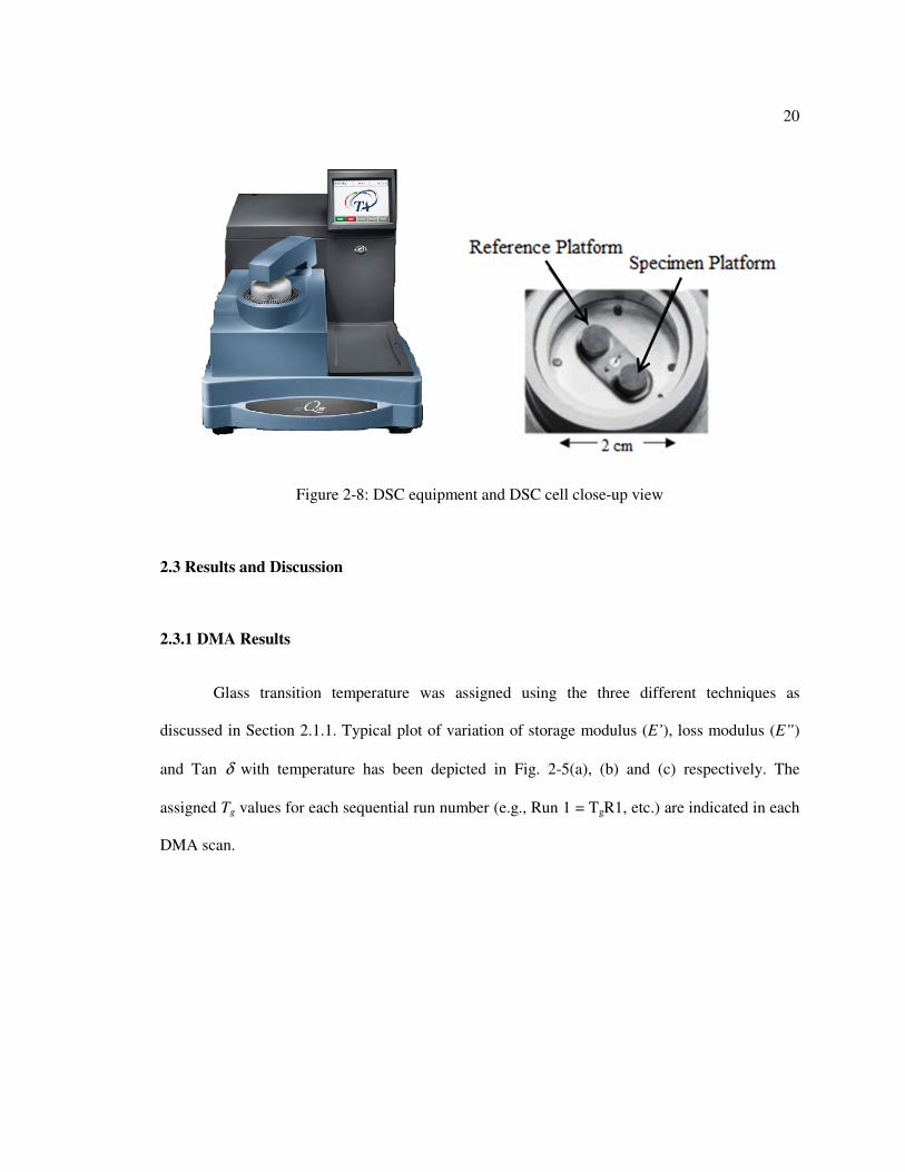
Figure 2-8: DSC equipment and DSC cell close-up view........................................................ 20

Figure 2-9: Typical repeated scans of (a) storage modulus, (b) loss modulus and Tan δ

for a 7-day-old resin specimen ......................................................................................... 21

Figure 2-10: Summary of first run DMA Tg data for epoxy cured for 7, 30 and 100 days

at room temperature, from batches A, B, and C. .............................................................. 22

Figure 2-11: Comparison of Tg for soaked and unhydrated specimens at different ages

using storage modulus (SM), loss modulus (LM) and Tan δ (TD) .................................. 26

Figure 2-12: Raw DMA data for a typical specimen soaked for 93 days ................................ 28

Figure 2-13: Two consecutive DSC scans on a 7-day-old specimen from Batch B’ ............... 29

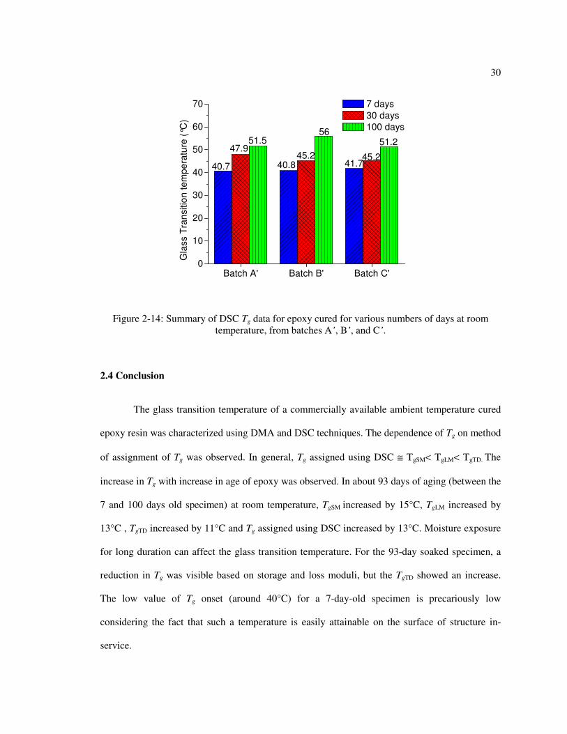
Figure 2-14: Summary of DSC Tg data for epoxy cured for various numbers of days at

room temperature, from batches A’, B’, and C’............................................................... 30

Figure 2-15: Enhancement in Tg using DMP 30 accelerator with generic resin mixture: (a)

EPON 862/IPDA; (b) EPON 862/IPDA/DMP 30. .......................................................... 31

Figure 3-1: (a) Specific volume variation with temperature and the deviation of specific

volume from equilibrium below Tg. (b) Variation of molecular mobility with specific

volume .............................................................................................................................. 35

viii

Figure 3-2: Evolution of enthalpy towards equilibrium (Stage A: Un-aged specimen,

Stage B: Partially aged specimen) and heat capacity curves at the two stages of

aging [26]. ........................................................................................................................ 37

Figure 3-3: Endothermic DSC peaks for fully cured Epon 828/MDA samples physically

aged at 130°C for aging times up to 648 hours (reproduced from [22]) .......................... 38

Figure 3-4: Graphical assignment of fictive temperature (Tf) (reproduced from [26]) ............ 39

Figure 3-5: DSC scans and heat of reaction value of freshly mixed resin at (a) 3°C/min

(b) 5°C/min (c) 8°C/min and (d) 10°C/min. .................................................................... 42

Figure 3-6: Degree of cure versus time at different heating rates ............................................ 43

Figure 3-7: Isoconversion curves of curing time and heating rate from DSC experimental

data ................................................................................................................................... 44

Figure 3-8: Dependence of fit parameters, P and Q, on degree of cure (α) ............................. 45

Figure3-9: Isoconversion map for MBrace saturant resin........................................................ 46

Figure 3-10 Residual enthalpy of a 7-day-old epoxy sample cured at 22°C temperature. ...... 47

Figure 3-11: Effect of 40°C exposure on Tg and residual cure enthalpy for resin aged for

10 days at room temperature. ........................................................................................... 48

Figure 3-12: Evolution of relaxation enthalpy for resin cured and .......................................... 49

Figure 3-13: Tg evolution with aging at different temperatures ............................................... 50

Figure 4-1: Typical creep response of viscoelastic material .................................................... 55

Figure 4-2: Time-temperature superposition to construct creep master curve......................... 58

Figure 4-3: Time aging time superposition to construct creep master creep compliance

curve [24] ......................................................................................................................... 60

Figure 4-4 Schematic showing temperature up-jump before creep testing of specimen to

simulate nonisothermal aging (reproduced from [39]) .................................................... 61

Figure 4-5 Sheet mold assembly .............................................................................................. 63

Figure 4-6 Lever arm creep frame ........................................................................................... 64

Figure 4-7: Wedge grip assembly with extensometers mounted specimen (left) and

custom-made clamp grip assembly (right). ...................................................................... 66

Figure 4-8: Summary of creep compliance versus time at 22°C ............................................. 69

Figure 4-9: Summary of creep compliance versus time at 30°C ............................................. 70

ix

Figure 4-10: Summary of creep compliance versus time at 35°C ........................................... 70

Figure 4-11: Representative creep compliance curves for 7-day-old specimens tested at

22°C, 30°C and 35°C. ...................................................................................................... 74


22°C, 30°C and 35°C ....................................................................................................... 75


22°C, 30°C and 35°C ....................................................................................................... 75

Figure 4-14: Best-fit functions for elastic modulus of epoxy resin at various ages and

temperatures ..................................................................................................................... 77

Figure 4-15: Tg evolution at different aging temperatures. ...................................................... 79

Figure 4-16: Piecewise power law fitted to average representative creep compliance

curve for 7-day-old specimen tested at 30°C ................................................................... 80

Figure 4-17 Creep compliance curves of 7-day-old epoxy resin tested at different

temperatures with points of β=0.965 marked .................................................................. 83

Figure 4-18: Graph for determination of activation energy at various β. ................................ 84

Figure 4-19: Variation of (Q/R) with “extent of aging” parameter β ...................................... 85

Figure 4-20: Creep prediction flowchart .................................................................................. 87

Figure 4-21: Model prediction for creep of 30D-22°C specimen ............................................ 88



Figure 4-24: Model prediction for creep of 100D-22°C specimen .......................................... 90



Figure B-1: Master creep curve for 7D-22°C-2 specimen. ...................................................... 127

Figure B-2: Logarithm of aging time and horizontal shift showing the constant rate of

increase of shift factor ...................................................................................................... 128

Figure D-1: First DSC scan showing the presence of physical aging in resin ......................... 134

Figure D-2: Second DSC scan after exposing the specimen to temperature above its

Tg..............................................................................................................................................134

x

LIST OF TABLES

Table 2-1: Dimensions of individual DMA specimens ........................................................... 17

Table 2-2: Tg assigned using storage modulus (TgSM) .............................................................. 23

Table 2-3: Tg assigned using loss modulus (TgLM) ................................................................... 23

Table 2-4: Tg assigned using Tan δ (TgTD) .............................................................................. 24

Table 2-5: Moisture content and first-run Tg for saturated specimens ..................................... 26

Table 4-1: Phenomenological models for modeling creep behavior ....................................... 56

Table 4-2: Number of specimens tested for each combination of age (prior to test) and

temperature during test ..................................................................................................... 67

Table 4-3: Summary of creep specimen dimensions and test stress levels .............................. 68

Table 4-4: Average representative creep compliance functions for various test conditions .... 72

Table 4-5: Elastic modulus of epoxy resin at different ages and test temperatures. ................ 76

Table 4-6: Fitted creep law parameters A and b for different ranges of creep time and

corresponding “extent of aging” parameter at 30°C ........................................................ 81

xi

ACKNOWLEDGEMENTS

I would like to express my sincere thanks to my advisor, Dr. C.E. Bakis for giving me an

opportunity to work on this thesis topic. As an individual, I have learnt a lot about discipline,

work ethics and passion for scientific research from him. I would also like to thank Dr. Lopez for

her constant guidance and encouragement during the research work. Being an interdisciplinary

research topic, her inputs were very valuable in completion of this thesis. I would like to

acknowledge the financial support of the National Science Foundation (grant CMMI-0826461),

the Penn State College of Engineering and the Department of Engineering Science and

Mechanics. The help and guidance of Dr. Brown and Dr. Hamilton by providing access to testing

facilities in their laboratory deserves to be acknowledged.

I would like to thank my friends and colleagues in my research group for their help and

support especially Jeff Flood, Yoseok Jeong and Ye Zhu. I would also like to thank my parents

and family members for their love and blessings during my stay at Penn State.

I am thankful to the faculty and staff members of the Engineering Science and Mechanics

Department, especially Mr. Ardell W. Hosterman and Mr. Scott Kralik, for helping me trouble-

shoot any technical problem in the laboratory.

1

Chapter 1

Introduction

Traditionally, civil infrastructures have been made out of masonry, concrete, timber, and

steel. With continuous research and development in the application of fiber reinforced polymer

(FRP) as a construction material, FRP has gained acceptance as a viable alternative. FRP material

is known for its high strength-to-weight ratio, high stiffness and good corrosion resistance. Thus,

the use of FRP enables reduction of dead weight of the structure and extends the life of the

structure. One of the applications of FRP is as externally bonded reinforcement to masonry,

concrete, timber, and steel structures. This application is becoming increasingly popular to repair

and strengthen a structure already in-service.

1.1 Externally Bonded FRP Reinforcement

The application of FRP as externally bonded reinforcement can be dated back to early

1980s. A good survey of the developments in the use of FRP reinforcement for civil infrastructure

can be found in literature [1-3]. Adhesively bonded precured FRP laminates were the first kind of

FRP strengthening system for concrete structures studied by Urs Meier and his team at the Swiss

Federal Lab for Material Testing and Research (EMPA). The use of FRP is advantageous as it

requires less installation time and labor in comparison to conventional methods like use of steel

plates or jackets for strengthening a structure. The externally bonded reinforcement is installed

either by adhering or mechanically fastening pre-cured FRP laminate or by actually applying and

curing the fabric and resin system in-situ by the hand layup technique. Hand lay-up technique

involves applying a thin layer of resin on the substrate and then installing layers of fabric,

2

saturated with resin on the substrate as shown in Figure 1-1. After curing, the fabric adheres to

the substrate, taking the form of the substrate on which it is laid. Externally bonded reinforcement

can be used for increasing load carrying capacity of structures in flexure, shear and also

compression when used to confine the structure.

Figure 1-1: Installation of flexural FRP reinforcement using hand layup technique

Near surface mounting (NSM) is a relatively new strengthening technique in which

precured FRP bars or strips is adhesively bonded to grooves cut into the concrete substrate. This

technique helps in protecting the bonded FRP from collision, high temperature and UV

degradation damage. The debonding strength is higher in comparison to externally bonded FRP

due to increased bonded area per unit length of reinforcement. However the NSM strengthening

technique requires preparation time and cutting of concrete cover may not always be feasible.

FRP consists of continuous fibers and polymeric resin matrix. The fiber used can be glass

carbon, aramid or high strength steel fiber. For externally bonded repair the fibers are woven or

stitched together to produce “fabric” which is saturated by the resin. The resin used can be an

3

epoxy resin, polyester resin or vinyl ester resin. Epoxy resins have better mechanical properties

than other two and are most commonly used. Fiber reinforced cementitious grout has also been

utilized as externally bonded strengthening system [4-5]. The use of cementitious grout as matrix

improves fire resistance of structure and resolves the problem of induced thermal stress between

FRP and concrete substrate.

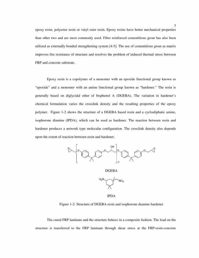
Epoxy resin is a copolymer of a monomer with an epoxide functional group known as

“epoxide” and a monomer with an amine functional group known as “hardener.” The resin is

generally based on diglycidal ether of bisphenol A (DGEBA). The variation in hardener’s

chemical formulation varies the crosslink density and the resulting properties of the epoxy

polymer. Figure 1-2 shows the structure of a DGEBA based resin and a cycloaliphatic amine,

isophorone diamine (IPDA), which can be used as hardener. The reaction between resin and

hardener produces a network type molecular configuration. The crosslink density also depends

upon the extent of reaction between resin and hardener.

DGEBA

IPDA

Figure 1-2: Structure of DGEBA resin and isophorone diamine hardener

The cured FRP laminate and the structure behave in a composite fashion. The load on the

structure is transferred to the FRP laminate through shear stress at the FRP-resin-concrete

4

interface. The shear stress at discontinuities in the substrate (e.g., concrete crack) or FRP (e.g.,

termination point) is relatively high due to stress concentration and decreases almost

exponentially away from the discontinuity, as shown in Figure 1-3 for the FRP termination point.

This high shear stress can result in debonding of FRP from the substrate, which is the most

common mode of failure of externally bonded FRP systems [2].

Figure 1-3: Schematic of load transfer in externally bonded FRP

1.2 Effect of Elevated Temperature and Sustained Loading

The FRP external strengthening system consists of glass or carbon fiber and, typically,

epoxy resin as the matrix and adhesive. The system is most often installed and cured at an

ambient temperature, although heating systems such as electrical heaters, infrared heaters and

heat blankets have been attempted with much higher installation cost. Heating devices which

utilizes electrical conductivity of carbon fibers to heat cure the CFRP laminate by passing electric

current have also been developed but are not commonly used [6]. Cooler temperatures slow the

curing process, while warmer temperatures accelerate it. The desired result of curing is a polymer

with rigid, or glassy, characteristics throughout the expected service temperature range. At

5

sufficiently high temperatures, polymers lose their desired glassy characteristic and behave as

rubbery materials [7]. This phenomenon is known as the glassy-rubbery transition. The transition

takes place over a range of 5-10°C. A particular temperature in this range is assigned as the glass

transition temperature (Tg). As epoxy resins used in FRP external strengthening applications are

typically cured at room temperature the extent of chemical cure is less than 100% [8]. The glass

transition temperature, which is dependent of the extent of chemical cure and the crosslink

density in the resin system, is generally close to the service temperature when the service

temperature is the only source of thermal energy for curing. At temperatures close to the Tg,

polymeric materials also exhibit considerable time dependent deformation under sustained

loading, also known as creep deformation. Hence to predict the effect of creep in FRP

strengthened concrete structures it is important to understand the combined effect of temperature

and sustained mechanical loading on the polymeric resin system.

The effect of elevated temperature on the bond properties of FRP externally bonded on

concrete structures has been reported in only a few publications [9][10][11]. Bakis [9] discussed

the importance of Tg in relation to elevated temperature capability and safety of structures. He

also discussed the various methods of assigning Tg and the variability in the assigned value of

glass transition temperature. Leone et al. [10] describe an experimental investigation carried out

on FRP strengthened concrete double-lap shear specimens tested at temperatures near and above

Tg. The maximum bond strength at the FRP-concrete interface decreased with increasing test

temperature. In specimens tested for bond strength at a temperature of Tg+20°C, loss of adhesion

at the FRP epoxy concrete interface and debonding of FRP from the substrate was observed.

Klamer et al. [11] also evaluated strength of double-lap shear specimens and reported an increase

in failure strength with increase in test temperature below Tg. At elevated temperature below Tg

6

the failure took place in the concrete near the interface. For temperatures above Tg, a decrease in

ultimate load was observed and failure took place exactly at the FRP-concrete interface.

The importance of combined sustained load and elevated temperature is underlined

considering results reported by Bakis [9]. Notched, plain concrete beams with externally bonded

carbon FRP (CFRP) tensile reinforcement were placed under a constant flexural load using

springs, as shown in Figure 1-4a, so that the fibers were under a tensile stress of about 50% of

ultimate. Following 1 to 6 days of exposure in the ambient summer weather (~40°C surface

temperature and ~80% relative humidity), the CFRP reinforcement catastrophically debonded at

the epoxy/concrete interface, as seen in Figure 1-4b. The reduction in physical properties of

epoxy resins over a temperature range associated with glass transition temperature, Tg, was

suspected to be the cause of the loss of bond strength. It is therefore critical to understand the

bond behavior FRP bonded to concrete at elevated temperatures and sustained loads.

(a) (b)

Figure 1-4: Sustained loading setup (a) and debonding failure mode (b) for plain concrete beams

with externally bonded CFRP reinforcement [9]

7

1.3 Motivation and Research Objectives

Detailed design guidelines for design of new and repair of old concrete structures with

externally bonded FRP have been developed. American Concrete Institute’s ACI 440.2R [12] and

European task group fib (International Federation for Structural Concrete) 9.3’s Bulletin 14 [6]

are two of the most widely used design guidelines for externally bonded FRP reinforcement. The

design guidelines lack substantial coverage of long term durability and effect of creep and

elevated temperature on FRP external strengthening systems.

The major objective of this investigation is to develop a model to predict creep in epoxy

resin used in FRP strengthening systems for a given mechanical and thermal loading history of

the epoxy resin. Such a model, when incorporated in a numerical code, can be used to predict the

long term response of structure subjected to sustained loading. It will be helpful in studying the

effect of creep at elevated temperature on the residual strength of FRP strengthened structures.

The investigation is focused on a commercially available epoxy resin system marketed to be used

as a fiber saturant and adhesive for installing externally bonded FRP systems onto concrete,

masonry, and timber. As the temperature capability of the composite repair system is dependent

on the glass transition temperature of the resin system used, the Tg of the resin is characterized at

ages of 7, 30 and 100 days. The Tg is characterized using two techniques—dynamic mechanical

analysis (DMA) and differential scanning calorimetry (DSC). DSC is used to further study the

evolution of Tg and physical and chemical aging kinetics in the epoxy resin used in the

investigation. Tensile creep behavior of the plain resin is studied at different temperatures and

ages. The observed creep behavior along with the knowledge of aging kinetics is used to develop

a predictive model for evaluating creep behavior in the resin.

8

Chapter 2

Characterization of Glass Transition Temperature

2.1 Introduction

Glass transition is an important phenomenon associated with viscoelastic materials like

polymeric resins. According to ASTM E1142 [13]—standard terminology relating to thermo-

physical properties—it is defined as “the reversible change in an amorphous material or in

amorphous regions of a partially crystalline material, from (or to) a viscous or rubbery condition

to (or from) a hard and relatively brittle one.” The glass transition is thermodynamically classified

as a second order transition or alpha transition in which there is no abrupt change in volume of

the material undergoing transition, unlike a melting point. As a material is heated through the

glass transition temperature, it exhibits large scale segmental motion of polymeric chains. At

temperatures lower than glass transition temperature polymers can exhibit localized motion of

polymer chains or side groups and are classified as sub-Tg transitions (beta and gamma

transition). The glass transition temperature of an epoxy polymer depends on the chemical

reactivity of the epoxide amine reaction at the temperature of cure. It is also dependent on the

time for cure. Increased cure time and temperature both increase the degree of cure, which in-turn

increases the glass transition temperature of epoxy. The present investigation focuses on ambient

temperature cured epoxy resin. As the epoxide (resin) and amine (hardener) are mixed, the

chemical reaction initiates and degree of cure starts to advance. When the degree of cure

advances to a stage where Tg starts exceeding the cure temperature, the epoxy resin vitrifies.

9

Vitrification of epoxy resin reduces the mobility of chains and reduces the rate of chemical

reaction which effects further advance of degree of cure and increasing of the Tg. Thus, with

ambient temperature cure it is difficult to achieve the maximum achievable Tg of the resin system.

For epoxy cured at ambient temperature, the Tg is also affected by the phenomenon of physical

aging or structural relaxation.

The glass transition occurs in a narrow temperature range. In general, a temperature

point within the narrow temperature range is used to specify the glass transition temperature. But,

since the glass transition phenomenon may itself occur over a range of several degrees, assigning

a singular temperature as Tg results in ambiguity. The glass transition phenomenon is observed by

measuring electrical, mechanical, thermal, or other physical properties which change significantly

over the transition temperature range. For example DSC (differential scanning calorimetry)

assigns Tg based on changes in specific heat capacity, TMA (thermo-mechanical analysis) assigns

Tg based on changes in coefficient of thermal expansion, and DMA (dynamic mechanical

analysis) assigns Tg by measuring changes in the dynamic stress-strain behavior. The Tg values

assigned using these different methods often differ from each other significantly and are

furthermore dependent on the procedural details within any one method.

The objective of the portion of the investigation described in this chapter is to assign

glass transition temperature to the resin and also study the evolution of Tg with age of resin. The

investigation also compares different methods of assignment of Tg. Another objective of this part

of the investigation is to study the effect of moisture on the Tg.

10

2.1.1 Assignment of Tg using DMA

As discussed above, DMA is one of the well-known experimental techniques for

determining the Tg of polymeric materials. DMA involves applying a stress (or strain) varying

sinusoidally in time and measuring the corresponding sinusoidal strain (or stress) magnitude and

phase shift. Time, temperature and loading frequency are the test parameters that can be varied

during DMA testing. ASTM E1640 [13] describes a standard test method for the assignment of

Tg by DMA for thermoplastic and thermosetting polymers and partially crystalline materials. In

the present investigation, fixed strain amplitude and frequency were applied as the temperature

was varied through the Tg. Due to the viscoelastic nature of the material, a phase difference exists

between the strain and stress in the specimen. The steady-state stress to strain ratio, E*, is

therefore a complex quantity having in-phase and out-of-phase components,

�∗ = �’ + ��” (2-1)

where E’ is the ratio of stress to in-phase strain and E” is the ratio of stress to 90° out-of-phase

strain. E’ is also known as the storage modulus as it relates to mechanical energy stored in the

material, whereas E” relates to viscous energy dissipated and is therefore known as the loss

modulus. The schematic depicted in Figure 2-1 shows the phasor relationships among E’, E” and

E*.

11

Figure 2-1: Relationship between storage E’, E” and E*

The Tg of a material can be assigned by the onset of the rapid loss of storage modulus

with increased temperature and by the peaking of the loss modulus over the glass transition

temperature range. The loss modulus can be determined by Equation 2-2, where Tan δ is known

as the loss factor and δ is the phase angle between the stress and strain.

�” = �’Tanδ (2-2)

The peak of a plot of Tan δ versus temperature can also be used to assign Tg. Thus, using a DMA

apparatus, one can assign the Tg based on a plot of the storage modulus, loss modulus, or Tan δ

versus temperature.

2.1.2 Assignment of Tg using DSC

Differential scanning calorimetry is a thermoanalytical technique which accurately

measures the heat inflow or outflow from a specimen when exposed to a controlled thermal

12

condition [14]. DSC is typically used to measure transition temperatures and heat of transition.

When a polymer undergoes a glass transition, the heat capacity of the specimen undergoes a step

change which is used to assign Tg. Figure 2-2 shows a typical DSC scan showing the step change

in heat flow as the experimental sample undergoes glass transition.

Figure 2-2: Typical DSC scan

Differential scanning calorimeters can be classified into two classes depending on their

working principle: power compensated DSC and heat flux DSC. The heat flux DSC consists of

sample and reference pan in the same furnace (as shown in Figure 2-3). The sample pan holds the

sample to be tested whereas the reference pan is empty. The sample and reference pan are

identical in all other respects. As the furnace is heated, the temperature difference between the

two pans is measured by thermocouples attached to the bases below each pan. The temperature

difference is converted into heat flow in or out of the sample pan using thermal equivalent

resistance of the base plate.

Glass Transition

Exothermic reaction

Endothermic reaction

He

at

Flo

w (

W)

E

xo u

p

Temperature (°C)

Baseline

13

Figure 2-3: Schematic representation of heat flux DSC

The power compensated DSC consists of two separate furnaces, each with its individual

heater and temperature sensor (as shown in Figure 2-4). The basic principle of operation of a

power compensated DSC is maintaining a “thermal null” system. As both the pans are heated at

the same rate, the amount of heat absorbed or released by the sample is reflected in the difference

in energy provided to the two pans.

Figure 2-4: Schematic representation of a power compensated DSC

DSC equipment should be calibrated using high purity substance with known thermal

properties. The procedures and guidelines for calibration have been discussed in-detail elsewhere

[14]. Two types of calibration are done on the DSC equipment—temperature calibration and

Sample Reference

Individual Heater

Temperature Sensor

14

caloric calibration. In the present investigation, high purity indium was used to check both

temperature and caloric calibration.

2.2 Experiments

A commercially available resin system used for saturating FRP strengthening system was

chosen for characterizing glass transition temperature using DMA and DSC. The product is

marketed by BASF chemicals (www.basf.com) and is sold under the brand name “MBrace

Saturant.” The resin is a two part epoxy resin with Bisphenol-A epoxy as the major constituent of

the “resin part” and isophoronediamine as the major constituent of the “hardener” part. The

application of this resin involves curing it at ambient temperature. Hence it is of interest to assign

the Tg and investigate the evolution of Tg for the resin system with age.

2.2.1 DMA Characterization of Tg

DMA testing was done on a TA Instruments Q800 dynamic mechanical analyzer in the

tensile mode. The Tg test sequence was determined according to ASTM E1640 (2004). The glass

transition temperature was assigned using each of the three methods as discussed earlier:

− Onset of decrease of the storage modulus, E’, versus temperature plot—i.e., the midpoint of

the temperature range over which the rate of decrease of E’ with increasing temperature

dramatically increases;

− Peak of the loss modulus, E”, versus temperature plot;

− Peak of the Tan δ versus temperature plot.

15

The resin was mixed in the proportion mentioned in manufacturer’s technical data sheet.

Upon completing the mixing procedure, the material was immediately placed in a vacuum

chamber and degassed in order to minimize the presence of air voids in the material. Degassing of

resin was an important aspect in specimen preparation since the specimen thickness was only

~0.3 mm and any air voids could change the specimen cross-sectional properties significantly.

The resin was molded between two steel plates held together by three layers of 0.1-mm-thick

double sided tape (Figure 2-5). These plates were submerged inside a Teflon container filled with

the material (Figure 2- 6) and then degassed in a vacuum chamber at ambient temperature for at

least 15 minutes. Silicone based mold release agent manufactured by Huron technologies was

used to prevent epoxy from adhering to the aluminum surface and to aid in easy removal of cured

sheets from the mold.

Figure 2-5: Steel mold for thin film specimen

16

Figure 2-6: Schematic diagram of Teflon mold for film specimen

To ensure some degree of assessment of batch-to-batch variability, three different batches

of resin were mixed and molded into thin films. One specimen was tested from each batch at each

target age. Films were allowed to cure for 7 days in the air-conditioned laboratory environment

before demolding them. Demolded films were cut into specimens of approximately 30 mm in

length, 5 mm in width, and 0.3 mm in thickness using a utility knife. The specimens and the

unused sheet of resin were stored in a desiccator with anhydrous calcium sulfate based desiccant.

Dimensions of individual specimens are tabulated in Table 2-1. The number in the specimen

nomenclature indicates the age of the specimen in days and the letter indicates the batch

identifier. For example, for the specimen named 30B, 30 represent age in days and B indicates the

batch name. Specimens were tested at the ages of 7, 30 and 100 days (130 days in one of the

batches).

Epoxy Resin

Steel plates sprayed

with release agent

Double sided tape

Teflon Container

17

Table 2-1: Dimensions of individual DMA specimens

Specimen Name Width (mm) Thickness (mm)

7A 5.35 0.28

7B 4.79 0.27

7C 5.98 0.35

30A 4.3 0.24

30A 4.68 0.33

100A 5.92 0.28

100B 5.1 0.26

130C 5.03 0.29

Specimen size is very important in testing material properties in the temperature-

controlled furnace used in the DMA. The temperature of a thick specimen may lag behind the

furnace temperature resulting in inaccurate measurement of mechanical properties with varying

temperature. Thinner specimens allow for less temperature variation between the specimen and

the point in the furnace where the feedback thermocouple is located.

The TA Instruments Q800 dynamic mechanical analyzer used in the present investigation

is a non-contact, linear drive motor device with optical encoding for strain detection. The DMA is

designed to take precise stress/strain measurements in a broad range of temperatures (-150 –

600°C). The device, as shown in Figure 2-7, has a furnace which allows the user to control

environmental conditions and has various clamp types for different testing needs. The present

tests have been done using tension clamps (Figure 2-7) and laboratory air environment inside the

test chamber. Heating elements and liquid nitrogen were used to carry out rapid temperature

changes. Due to the precision of the instrument, routine calibration needed to be performed before

each test.

18

Figure 2-7: DMA equipment and thin film resin specimen gripped in the tension film clamp

The Tg test sequence was determined according to ASTM E1640 (2004) [13]. The tests

were run using a constant maximum strain excursion of 0.05% and a frequency of 5 Hz. After

DMA calibration, the following test sequence was followed.

Upon closing the furnace, temperature was equilibrated at -50°C and then held at constant

temperature for 10 minutes. Temperature decreases were done at uncontrolled rates. No data

was collected during this time period. Data storage then began and the temperature was ramped

up at a rate of 3°C per minute until 120°C was reached. Data storage was then turned off. This

cycle was repeated for three or six cycles per specimen.

A limited investigation of the effect of moisture on Tg of epoxy was also carried out. Thin

film specimens of average thickness 0.2-0.3 mm were molded and cured at room temperature for

7 days. After 7 days of curing, DMA specimens were immersed in de-ionized water at room

temperature. Three batches of resin, namely Ah, Bh, Ch were mixed and molded into film

19

specimen. A saturation moisture content of approximately 2.5% by weight was attained after 3

days in water. DMA scans, following the same test sequence as mentioned above, were done at

ages of 30 days (23 days in water) and 100 days (93 days in water). Specimens were removed

from the water and then wiped with paper towel to remove excess water from surface before

gripping them in the DMA apparatus.

2.2.2 DSC Characterization of Tg

DSC tests were utilized to study the glass transition temperature. A TA Instruments Q100

DSC—a heat flux type DSC—was used in the present investigation. ASTM D3418-08 [15] was

followed to assign the Tg. A sample mass of about 5 mg was used in each scan. Large volume

stainless steel pans of 60 µL capacity manufactured by Perkin Elmer with a lid and rubber seal

capable of sustaining high internal pressure were used in the scans to prevent any leakage of

volatiles. The steel pans are placed over two circular raised pedestals as shown in Figure 2-8.

Scans were done at 3°C/min from 0°C to 250°C after equilibrating the samples at 0°C in a

nitrogen gas environment. In a few cases, the specimen was exposed to two consecutive heat-cool

cycles. Heating was done at 3°C/min from 0° to 250°C and cooling was done at 10°C/min from

250°C back to 0°C. To account for asymmetry in the measuring system, DSC scans with

two empty pans were run to obtain what is known as the “zero line.” The zero line was

subtracted from the scan data to obtain the actual heat flow to and from the test sample.

DSC scans were done for three different batches (A’, B’, and C’) at age of 7, 30 and 100 days.

These batches primed since they are not the same batches used in the DMA tests.

20

Figure 2-8: DSC equipment and DSC cell close-up view

2.3 Results and Discussion

2.3.1 DMA Results

Glass transition temperature was assigned using the three different techniques as

discussed in Section 2.1.1. Typical plot of variation of storage modulus (E’), loss modulus (E”)

and Tan δ with temperature has been depicted in Fig. 2-5(a), (b) and (c) respectively. The

assigned Tg values for each sequential run number (e.g., Run 1 = TgR1, etc.) are indicated in each

DMA scan.

21

(a) (b)

(c)

Figure 2-9: Typical repeated scans of (a) storage modulus, (b) loss modulus and Tan δ

for a 7-day-old resin specimen

It can be seen that Tg increases with each thermal sweep cycle. This could be due to

“post-curing” of the resin. As the specimen is heated above Tg molecular chains regain their

mobility and unreacted epoxide and amine can undergo chemical reaction improving the crosslink

density and hence increasing the Tg in next run. This also supports the argument that ambient

temperature cured epoxy is not 100% chemically cured. For few of the DMA scans six

consecutive scans were done quantify the maximum attainable Tg. The storage modulus, loss

-50 -30 -10 10 30 50 70 90 110 130

0

1

2

3

4

5

TgR3=59°C

Run 1

Run 2

Run 3

TgR2=50°CS

tora

ge M

odulu

s (

GP

a)

Temperature (°C)

TgR1=43°C

-50 -30 -10 10 30 50 70 90 110 130

0.00

0.05

0.10

0.15

0.20

0.25

0.30

0.35

0.40

0.45 Run 1

Run 2

Run 3 TgR3=76°C

TgR2=67°C

Lo

ss M

od

ulu

s (

GP

a)

Temperature (°C)

TgR1=49°C

-40 -20 0 20 40 60 80 100 120 140

0.0

0.2

0.4

0.6

0.8

1.0

1.2

1.4

1.6 Run 1

Run 2

Run 3

TgR3=92°C

TgR2=85°C

Ta

n δ

Temperature (°C)

TgR1=60°C

22

modulus and Tan δ for all DMA scans have been included in Appendix A. The summary of glass

transition temperature assigned using three different methods at different ages—7, 30 and 100

days for the first run has been shown in Figure 2-10. For one particular batch specimen were

tested at age of 130 days. The Tg value assigned for all specimens in different runs using storage

modulus, loss modulus and Tan δ have been tabulated in Tables 2-2, 2-3 and 2-4. Also included

in the tables are the actual ages of the specimens when tested (as part of the specimen name).

Figure 2-10: Summary of first run DMA Tg data for epoxy cured for 7, 30 and 100 days

at room temperature, from batches A, B, and C.

7 days 30 days 100 days

10

20

30

40

50

60

70

80

A B C A B CA B C

Storage Modulus

Loss Modulus

Tan δ

Gla

ss T

ransitio

n T

em

pe

ratu

re (

°C)

Age of Specimen

23

Table 2-2: Tg assigned using storage modulus (TgSM)

Specimen TgSM (°C)

R1 R2 R3 R4 R5 R6

7A 42 50 61 * * *

7B 43 50 59 62 63 64

7C 36 46 57 58 65 65

Average

at 7days 40 49 59 60 64 64

30A 51 66 63 * * *

30B 48 51 59 60 65 66

30C 48 53 59 63 64 65

Average

at 30 days 49 57 60 61 64 65

100A 59 57 62 64 67 67

100B 52 55 60 64 65 66

Average at

100 days 55 56 61 64 66 66

130C 50 54 59 63 65 66

Table 2-3: Tg assigned using loss modulus (TgLM)

Specimen TgLM (°C)

R1 R2 R3 R4 R5 R6

7A 47 65 74 * * *

7B 49 67 76 79 82 83

7C 44 66 74 78 79 80

Average at

7days 47 66 75 78 80 81

30A 56 71 77 * * *

30B 51 69 75 79 80 81

30C 53 69 75 78 79 80

Average at

30 days 53 70 76 78 79 80

100A 64 72 78 80 81 82

100B 56 70 76 78 80 81

Average at

100 days 60 71 77 79 80 81

130C 56 70 77 79 79 80

24

Table 2-4: Tg assigned using Tan δ (TgTD)

Specimen TgTD (°C)

R1 R2 R3 R4 R5 R6

7A 59 86 93 * * *

7B 60 85 92 95 96 96

7C 57 84 91 93 94 95

Average at

7 days 59 85 92 94 95 95

30A 65 85 92 * * *

30B 63 86 92 94 95 95

30C 64 85 91 93 95 95

Average at

30 days 64 85 92 93 95 95

100A 73 88 93 95 96 97

100B 66 85 91 93 94 94

Average at

100 days 69.5 86 92 94 95 95

130C 67 85 92 94 95 95

It can be seen that Tg assigned using storage modulus (TgSM), loss modulus (TgLM) and Tan

δ (TgTD) follow the trend TgSM < TgLM < TgTD. Assignment of Tg using Tan δ and loss modulus

peaks are the more prevalent methods reported in the literature as they are relatively easier to pick

and more consistent. Finding Tg from the storage modulus is relatively operator-dependent

because of the need to manually fit tangents to the regions below and through the Tg range.

ASTM E1640 [13] recommends assigning Tg based on the point of intersection of these tangents,

which represents the center of the range of temperatures corresponding to the onset of transition.

On the other hand, the loss modulus and Tan δ peaks generally represent the midpoint

temperature of the temperature range over which transition takes place [7], at which point the

storage modulus may have lost half or more of its value just below Tg. From a structural

engineer’s point of view, a temperature which marks the onset of loss in storage modulus may be

25

the more appropriate upper use temperature, rather than the one at which the storage modulus has

been diminished substantially.

Referring to Figure 2-10, an increase in first-run Tg with age of epoxy was observed. In

about 93 days of aging (the number of days between the 7- and 100-days-old specimens) at room

temperature, TgSM increased by 15°C, TgLM increased by 13°C and TgTD increased by 11°C. The

reason for the increase in Tg of the ambient temperature cured epoxy aging at ambient

temperature will be discussed in Chapter 3. The first-run average Tg of a 7-day-old specimen

based on storage modulus was 40°C. It is precariously low, since a temperature near 40°C is

easily attainable on the surface of structure in-service. According to the ACI 440.2R-08

guidelines [12], the anticipated service temperature of an FRP system is recommended to not

exceed (Tg – 15)°C”. It should be noted that ACI 440.2R-08 defines Tg based on the loss modulus

method, although the guide is silent on the age of the material at the time of testing. The dry Tg is

used for dry conditions, and the wet Tg is used for wet conditions. For the test method employed

in the present investigation, the average dry TgTD value is 59°C for a 7-day-old specimen. Thus,

the service temperature limit for the subject resin system according to ACI is 44°C if the Tg is to

be based on 7-day-old material. The fib Bulletin 14 has a similar guideline for Tg of resin in

relation to the service temperature of the structure. The fib Bulletin 14 recommends assigning Tg

using the DSC technique but has no guidelines with respect to the age of testing or conditioning

of specimen prior to testing. According to the guideline, the service temperature should not

exceed (Tg – 20)°C and a minimum absolute value of 45°C. Hence owing to the low Tg value, use

of a 7-day-old cured resin could severely limit the upper use temperature of the structure.

The effect of moisture on the Tg was also evaluated. The average Tg for three batches of

epoxy tested at ages of 30 days (23 days in water) and 100 days (93 days in water) are reported in

26

Figure 2-11 alongside results for dry (unhydrated) epoxy specimens of similar total age. The Tg

assigned for individual specimens using the first DMA scan with respective saturation moisture

contents has been tabulated in Table 2-5.

Figure 2-11: Comparison of Tg for soaked and unhydrated specimens at different ages

using storage modulus (SM), loss modulus (LM) and Tan δ (TD)

Table 2-5: Moisture content and first-run Tg for saturated specimens

Specimen Saturation Moisture

Content (% by weight) TgSM (°C) TgLM (°C) TgTD (°C)

30Ah 3.0 47 53 78

30Bh 2.4 46 52 77

30Ch 2.8 52 59 85

Average 30

days 2.7 48 55 80

100Ah 2.5 49 55 81

100Bh 2.6 51 55 82

100Ch 2.4 49 54 80

Average 100

days 2.5 50 55 81

SM LM TD

40

50

60

70

80

90

23 days exposure

Tg (

°C)

SM LM TD

40

50

60

70

80

Unhydrated specimen

Soaked in deionized H2O

Tg (

°C)

93 days exposure

27

Referring to Figure 2-11, it can be seen that the Tg of 23-day soaked specimens is

comparable to the equivalently aged unhydrated specimens based on storage modulus, whereas it

is higher than the unhydrated specimens based on loss modulus and Tan δ. An increase in Tg with

moisture content has been reported previously. According to Wu et al. [17], the presence of water

(up to 2 weight %) accelerates the curing rate and the evolution of Tg in epoxy resins. Further

studies need to be done to check if the increase in Tg is actually due to the progress of a chemical

reaction or some other mechanism in the current epoxy resin. For the 93-day soaked specimen, a

reduction in Tg was visible based on storage and loss moduli, but the TgTD indicated an increase.

The Tan δ curve had an obscured peak at around 65°C (Figure 2-12). Yang et al. [18]

have also reported the splitting of Tan δ peaks in aqueous solution. The splitting can be attributed

to plasticization of epoxy in water or non-uniform drying during DMA testing, with the obscured

peak associated with the Tg of a “wetter” phase and the higher peak being Tg of a “drier” phase. It

is also interesting to note that the Tg assigned according to the Tan δ peak can be deceptive, as the

storage modulus of the material decreases considerably at 25°C below the TgTD.

28

Figure 2-12: Raw DMA data for a typical specimen soaked for 93 days

2.3.2 DSC Results

A typical DSC scan (after subtracting the zero line) of a 30-day-old resin sample is

shown in Fig. 2-13. The base lines before and after the transition are marked. These extended

baselines intersected the line of greatest slope in the transition region at two points. The

temperature at the point on the curve corresponding to average of heat flow at these two points

was assigned as the glass transition temperature. Figure 2-13 shows a typical DSC scan on a 7-

day-old epoxy specimen. The specimen was exposed to two consecutive heat-cool cycles (as

discussed in Section 2-2-2). During the first thermal cycle, the specimen undergoes a glass

transition at around 40°C. An endothermic peak was also recorded in the thermogram as the

specimen undergoes glass transition. This peak is most probably a structural relaxation peak

generally associated with epoxy resin aged at a temperature below the Tg. As the specimen is

heated further (during the first cycle) two exothermic peaks were observed. Exothermic peaks

0 20 40 60 80 100 1200.0

0.1

0.2

0.3

0.4

0.5

0.6

0.7

0.8 Storage Modulus

Loss Modulus

Tan δ

(Sto

rag

e M

odu

lus (

GP

a))

/10

Loss M

odu

lus (

GP

a)

Temperature (°C)

Tan δ

Hidden Peak

0.0

0.1

0.2

0.3

0.4

0.5

0.6

0.7

0.8

29

indicate chemical reaction of epoxy and amine chemical groups. During the second cycle, no

structural relaxation peak was observed as the heating of specimen above Tg during the first cycle

erases the effect of physical aging. The increase in Tg (from 41°C to 69°C) due to post curing of

resin during heating of specimen can also be seen.

Figure 2-13: Two consecutive DSC scans on a 7-day-old specimen from Batch B’

Figure 2-14 shows a comparison of Tg of three different batches of resin (A’, B’ and C’)

tested at ages of 7, 30, and 100 days. The assigned Tg increases with age of the epoxy, as was

observed using the DMA technique. The average Tg increased from 40°C to 53°C with the

increase in age from 7 days to 100 days. The Tg assigned using DSC was close to the TgSM

assigned using DMA. The low value of Tg at the age of 7 days (approximately 40°C) is especially

of concern for structural strengthening.

0 50 100 150 200 250

-2

-1

0

1

2

3

4

Run 2

TgRun2'=63°C

TgRun2=69°C

TgRun1'=55°CH

ea

t F

low

(m

W)

Temperature (°C)

TgRun1=40.8°C

Exo

Up

Run 1

Structural relaxation peak

Specimen

Mass=4.6 mg

30

Figure 2-14: Summary of DSC Tg data for epoxy cured for various numbers of days at room

temperature, from batches A’, B’, and C’.

2.4 Conclusion

The glass transition temperature of a commercially available ambient temperature cured

epoxy resin was characterized using DMA and DSC techniques. The dependence of Tg on method

of assignment of Tg was observed. In general, Tg assigned using DSC ≅ TgSM< TgLM< TgTD. The

increase in Tg with increase in age of epoxy was observed. In about 93 days of aging (between the

7 and 100 days old specimen) at room temperature, TgSM increased by 15°C, TgLM increased by

13°C , TgTD increased by 11°C and Tg assigned using DSC increased by 13°C. Moisture exposure

for long duration can affect the glass transition temperature. For the 93-day soaked specimen, a

reduction in Tg was visible based on storage and loss moduli, but the TgTD showed an increase.

The low value of Tg onset (around 40°C) for a 7-day-old specimen is precariously low

considering the fact that such a temperature is easily attainable on the surface of structure in-

service.

Batch A' Batch B' Batch C'0

10

20

30

40

50

60

70

51.2

45.241.7

56

45.240.8

51.547.9

Gla

ss T

ran

sitio

n t

em

pe

ratu

re (

°C)

7 days

30 days

100 days

40.7

31

A limited investigation to enhance the Tg of a generic epoxy resin system was made in the

present investigation. For this purpose, a commercially available accelerator for epoxy-amine

reactions known as DMP 30 (2,4,6-tris (dimethylaminomethyl) phenol) was used. The

formulation ratio for EPON 862 epoxide and isophorone diamine (IPDA) was worked out to be

25.19 grams of IPDA per 100 grams of EPON 862 epoxide. To accelerate the cure and generate

an increased temperature due to the exothermic conditions, 1.5% by volume of DMP 30 was

added to this generic resin formulation. A significant increase of in DSC Tg for a 7-day-old

specimen was observed, as shown in Figure 2-15. But there was a trade-off in the toughness of

the resin. The resin specimen molded using the mixture of EPON862/IPDA/ DMP 30 accelerator

was actually susceptible to cracking when attempts were made to machine specimens using the

as-cast plate.

(a) (b)

Figure 2-15: Enhancement in Tg using DMP 30 accelerator with generic resin mixture: (a)

EPON 862/IPDA; (b) EPON 862/IPDA/DMP 30.

Although the increase in Tg looked promising, better results may have been obtained if

additional time was spent on toughening the system with modifiers. Further exploration of this

approach for increasing the Tg of ambient-cured epoxy is left for future work.

0 40 80 120 160 200-1.00

-0.75

-0.50

-0.25

0.00

0.25

0.50

He

at

Flo

w (

W/g

)

Temperature (°C)

Exo

Up

Tg=40°C

0 40 80 120 160 200-1.0

-0.5

0.0

0.5

1.0

1.5

He

at

Flo

w (

mW

)

Temperature (°C)

Exo

Up

Tg=53.4°C

32

Chapter 3

Investigation of Cure Kinetics and Physical Aging Kinetics in Epoxy Resin

3.1 Introduction

The importance of Tg in relation to service temperature has been emphasized in Chapter

2. The Tg can be enhanced by post curing the resin or by physical aging of resin below its Tg.

Chemical curing improves the cross link density in the network polymers and hence effects the

polymer’s properties. Physical aging also affects the physical properties of the resin. The

chemical cure kinetics and physical aging kinetics can impact the Tg evolution and creep

properties of epoxy resin. Hence, it is important to understand and model the phenomena of

chemical cure and physical aging in the resin system under study.

3.1.1 Literature Review on Cure Kinetics of Epoxy Resin

The kinetics of polymerization reactions in epoxy resins has been studied by several

authors [19-23]. For this purpose, several techniques such as differential scanning calorimetry

(DSC), infrared spectroscopy, dielectric spectroscopy and dielectric thermal analysis have been

used. Isothermal and non-isothermal DSC are the most commonly used techniques to model the

epoxy cure kinetics. The degree of cure (α) of epoxy is the extent of completion of the

polymerization reaction. It is expressed in terms of the heat released during the reaction as

� = ∆��

∆�� (3-1)

33

where ∆�� is the maximum possible heat of reaction of the epoxy-amine reaction and

∆�� ! is the actual amount of heat released by the epoxy-amine system. The value of

∆�� is dependent on the stoichiometry of the reactants. A stoichiometric ratio of reactants,

such that all the reactants are converted into products will give the maximum value of ∆��.

Hence a freshly mixed resin has a degree of cure value of 0 and a fully cured resin has a degree of

cure value as high as 1. Cure kinetics are often mathematically expressed in terms of rate of

change of degree of cure with time (# � #$)⁄ , also known as the “rate of conversion.” Several

phenomenological models have been developed and used to model cure kinetics. The nth order

reaction model is the simplest model which expresses rate of conversion as in Equation 3-2,

'('�

= )(1 − �)! (3-2)

where K is a rate constant with an Arrhenius-type dependence on temperature [21]. Epoxy-amine

reactions have also been modeled using the Kamal and Sourour model, which assumes the

reaction to be autocatalytic in nature,

'('�

= (,- + ,.�/)(1 − �)! (3-3)

where k1 and k2 are empirically determined rate constants [19][21].

Ruiz et al. [23] describe the “isoconversion map” technique which uses DSC

measurements to graphically predict the degree of cure in thermosetting polymers for varied

thermal histories. This technique overcomes the complication of fitting a multi-parameter kinetics

model to experimentally obtained data since it requires no model fit whatsoever. In the present

investigation, this technique has been adopted to model the cure kinetic behavior for the epoxy

34

resin system under investigation. Detailed treatment of experimental data to develop iso-

conversion maps is discussed in a subsequent section.

3.1.2 Literature Review on Physical Aging Kinetics of Epoxy Resin

The phenomenon of physical aging has been comprehensively reviewed and discussed by

several authors [24-26]. The term physical aging was first used by Struik [24] to describe the

gradual evolution of glassy polymer towards equilibrium. Struik [24] explains the phenomenon of

physical aging based on the concept of free volume and molecular mobility. Molecular mobility

is defined as the rate at which the molecular chain configuration changes. Free volume refers to

the empty spaces in the molecular arrangement. As the polymer is stored at a temperature below

its Tg , the free volume starts decreasing towards the equilibrium value as depicted from the plot

of specific volume versus temperature (Figure 3-1a). In-turn, the reduction of free volume

decreases the mobility of the molecular chain (Figure 3-1b) which decreases the rate of change of

free volume with time. This cyclic process goes on until an equilibrium molecular configuration

is achieved asymptotically. Physical aging affects several experimentally measurable properties

such as specific volume, enthalpy, elastic modulus, creep response, and dielectric properties of

the polymer.

35

(a) (b)

Figure 3-1: (a) Specific volume variation with temperature and the deviation of specific volume

from equilibrium below Tg. (b) Variation of molecular mobility with specific volume

Struik [24] also explained the importance of taking physical aging into consideration in

the testing of plastics and studying of long term performance of polymeric materials. Hutchinson

[26] has reviewed dilatometry and DSC techniques to characterize physical aging. Dilatometry or

volume relaxation measurement, which involves measuring change in length or volume of the

polymer, was one of the earliest techniques used to characterize physical aging. Based on

dilatometric studies, the non-linearity of isothermal aging with respect to departure from

equilibrium has been observed. Another important characteristic of physical aging is its

thermoreversiblity [24]. Heating a polymeric material to above its Tg brings it in equilibrium (as

shown in Figure 3-1) and erases any prior physical aging history of the material. Further storing

the material at temperature below Tg initiates the phenomenon of physical aging once again. In

this respect physical aging is different from chemical aging which is not thermoreversible.

Differential scanning calorimetry has become a popular technique to characterize and

study the phenomenon of physical aging. As the polymer is aged at temperature below Tg , the

36

enthalpy of the polymer starts decreasing towards the equilibrium enthalpy value. Figure 3-2

(reproduced from Hutchinson [26]) shows the specimen being aged at temperature Ta and the

decrease in enthalpy from Ho (point A) to Ht (point B) in time t. The decrease in enthalpy (Ht - Ho)

is equal to the difference of area under the endothermic relaxation peak on the DSC curves

corresponding to specimen at point A and point B. As the enthalpy of polymer decreases towards

the equilibrium value, the area under the endothermic relaxation peak of DSC curve also known

as the relaxation enthalpy (∆H) increases. Relaxation enthalpy has been used to study physical

aging kinetics of epoxy resin [28-30]. Plazek and Frund [30] showed the variation of relaxation

enthalpy with increase in aging time for a fully cured Epon 828/MDA epoxy resin samples

physically aged at 130°C (Figure 3-3). The paper also discusses the linearity of endothermic peak

areas with the logarithm of aging time. The temperatures corresponding to the peak of relaxation

enthalpy and onset of glass transition temperature have also been reported to evolve linearly with

the logarithm of aging time [29][30]. Hence, the onset of Tg can also be used as a measure of

physical aging.

37

Figure 3-2: Evolution of enthalpy towards equilibrium (Stage A: Un-aged specimen,

Stage B: Partially aged specimen) and heat capacity curves at the two stages of aging [26].

38

Figure 3-3: Endothermic DSC peaks for fully cured Epon 828/MDA samples physically

aged at 130°C for aging times up to 648 hours (reproduced from [22])

To explain the kinetics of physical aging, Tool [27] conducted dilatometric experiments

on inorganic glasses. The concept of fictive temperature (Tf) was introduced to explain the

dependence of aging kinetics on aging temperature, Ta, and the instantaneous state or structure of

the glass. Fictive temperature is defined as the temperature at which the aging material has the

same structure as the material in equilibrium if it was instantaneously cooled to equilibrium. It is

an artificial temperature which is equal to the glass transition temperature when aging time is zero

and equal to aging temperature at infinite aging time. Figure 3-4 (reproduced from [27) shows

how Tf is assigned for an aging material where l0 is the initial length, lt is the length after aging

time t, and l∞ is the equilibrium length at aging temperature Ta.

En

do

Up

39

Figure 3-4: Graphical assignment of fictive temperature (Tf) (reproduced from [26])

Structural relaxation kinetics is studied by variation of physically measurable quantities

such as enthalpy, specific volume or length from initial value to the equilibrium value. The

process of structural relaxation is characterized by a single relaxation time τ or a distribution of

relaxation times. Tool’s concept of fictive temperature was further developed by Moynihan et al.

[31] to give an expression for structural relaxation time which is known as the Tool,

Narayanaswamy, and Moynihan model or the TNM model. The TNM model expresses relaxation

time as a function of aging temperature, Ta, and fictive temperature, Tf, according to Equation (3-

4)

τ01, 134 = τ5 exp9:∆;∗<= + (->:)∆;∗

<=?@ (3-4)

The parameter x defines the relative contribution of temperature and structure on the relaxation

time. Parameter τ5is the relaxation time in equilibrium at infinitely high temperature, and∆A∗is

the apparent activation energy. The deviation of the measured property from its value at

40

equilibrium is denoted by δ. For example, if the measured property is enthalpy (H), δ is given

according to Equation (3-5)

δ = (�� − �B)/�B (3-5)

where �B is the equilibrium value of enthalpy. The relation between the deviation from

equilibrium,δ($), and relaxation time, τ, is given according to a stretched exponential function

also known as Kohlarausch-Williams-Watts function, where δ5is the initial value of δ($)

δ($) = δ5 exp[−(D #$

τ)

�

5

E@

(3-6)

The TNM parameters (x,β,∆A∗,τ5) are dependent on material being studied and are obtained by

an appropriate analysis of the experimental data.

3.2 Experimental Program

The experiments for studying kinetics of chemical cure and physical aging were done

using differential scanning calorimetry on MBrace Saturant

(BASF Corporation) epoxy resin.

The experimental procedures are discussed in the following sections.

3.2.1 Chemical Cure Kinetics

The investigation on cure kinetics was done by using differential scanning calorimetry to

study the progress of chemical cure by heating freshly mixed epoxy resin at different heating

rates. The enthalpy of reaction between epoxide and amine group was measured using DSC scans

done at different heating rates. By studying the progress of the chemical reaction at different

41

heating rates, a model to predict the degree of cure (α) after a given thermal exposure can be

developed. In the present study, Perkin Elmer’s DSC 8500—a power compensated DSC—was

used. Large volume stainless steel pans (Perkin Elmer) of 60 µL capacity with a lid and rubber

seal capable of sustaining high internal pressure was used in the scans. Thermal scans were done

at 3°C/min, 5°C/min, 8°C/min and 10°C/min from 0°C to 200°C. Specimen mass of around 5 mg

was used in every scan.

3.2.2 Physical Aging Kinetics

To study physical aging kinetics, differential scanning calorimetry was utilized. The DSC

scans were done at 3°C/min from 0°C to 80°C as the interest was in studying the phenomena of

glass transition and endothermic relaxation peak near Tg to characterize physical aging. A

separate investigation to check the thermoreversiblity of physical aging was done which has been

included in Appendix D.

3.3 Results and Discussion

This section presents the results of the investigation on chemical cure kinetics and

physical aging kinetics for the epoxy resin under study.

3.3.1 Model for Prediction of Degree of Cure (α)

The results for the DSC scan on freshly mixed epoxy at different scanning rates of

3°C/min, 5°C/min, 8°C/min and 10°C/min are shown in Figure 3-5. The DSC scans have their

baselines tilted as baselines were not subtracted in the data shown. Figure 3-5 shows a double

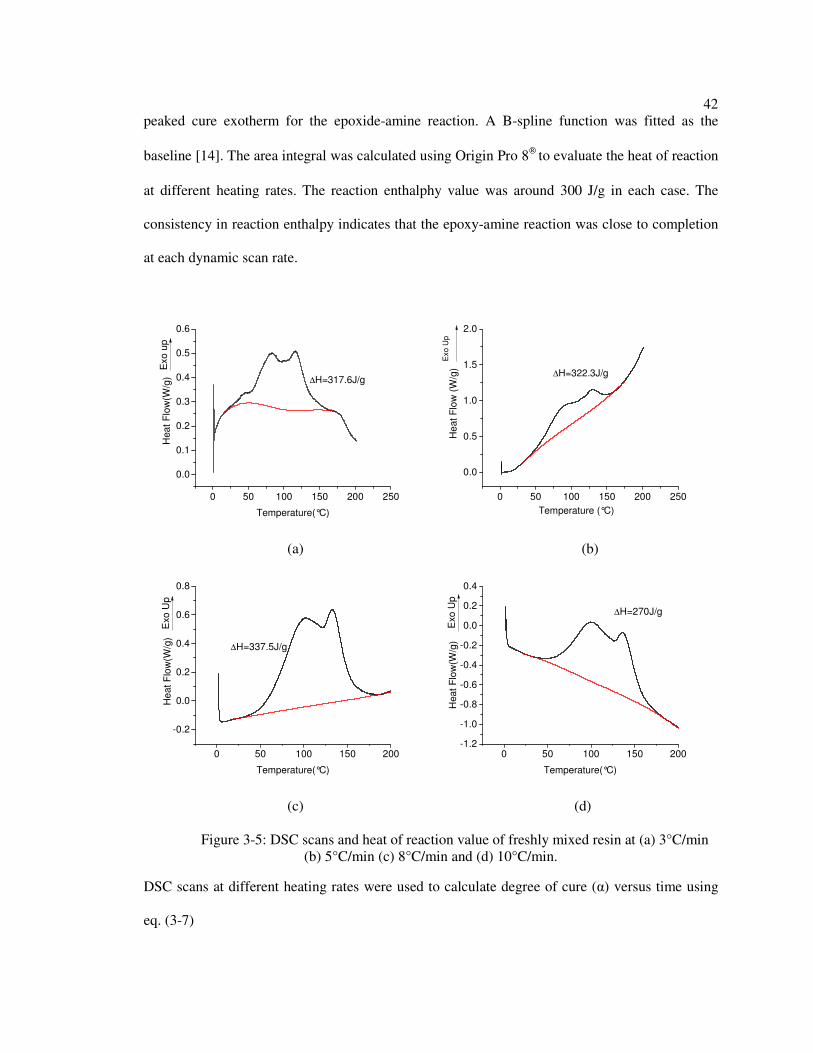
42

peaked cure exotherm for the epoxide-amine reaction. A B-spline function was fitted as the

baseline [14]. The area integral was calculated using Origin Pro 8

to evaluate the heat of reaction

at different heating rates. The reaction enthalphy value was around 300 J/g in each case. The

consistency in reaction enthalpy indicates that the epoxy-amine reaction was close to completion

at each dynamic scan rate.

(a) (b)

(c) (d)

Figure 3-5: DSC scans and heat of reaction value of freshly mixed resin at (a) 3°C/min

(b) 5°C/min (c) 8°C/min and (d) 10°C/min.

DSC scans at different heating rates were used to calculate degree of cure (α) versus time using

eq. (3-7)

0 50 100 150 200 250

0.0

0.1

0.2

0.3

0.4

0.5

0.6

Hea

t F

low

(W/g

)

Temperature(°C)

∆H=317.6J/g

Exo

up

0 50 100 150 200 250

0.0

0.5

1.0

1.5

2.0

∆H=322.3J/g

He

at

Flo

w (

W/g

)

Temperature (°C)

Exo U

p

0 50 100 150 200

-0.2

0.0

0.2

0.4

0.6

0.8

He

at

Flo

w(W

/g)

Temperature(°C)

∆H=337.5J/g

Exo

Up

0 50 100 150 200-1.2

-1.0

-0.8

-0.6

-0.4

-0.2

0.0

0.2

0.4

Hea

t F

low

(W/g

)

Temperature(°C)

∆H=270J/g

Exo

Up

43

�($) = F�F��

(3-7)

where G�� corresponds to the total area under DSC curve and G� is the partial area under DSC

curve up to time t. Figure 3-6 shows the degree of cure versus time plot for different heating rates.

Figure 3-6: Degree of cure versus time at different heating rates

The isoconversion modeling technique as reported by Ruiz et al. [23] was followed to

develop the prediction model for degree of cure. The method is called “iso-conversion technique”

because it evaluates the point with same degree of cure on DSC curves but at different time and

temperatures and then uses it to predict the time-dependent variation of degree of cure at different

heating rates or at different isothermal conditions. The time-heating rate function for constant

degree of cure (α) can be expressed as

0.0

0.2

0.4

0.6

0.8

1.0

1.2

0 10 20 30 40 50 60

3°C/min

5°C/min

8°C/min

10°C/min

Time (Minutes)

De

gre

e o

f C

ure

(α

)

44

log-5($) = K log-5 φL (3-8)

where t is time, φ is the heating rate in °C/min, and P and Q are two constants dependent on

degree of cure, α. From the degree of cure versus time plot (Figure 3-6), curing time values

corresponding to constant degrees of cure for different heating rates were picked. For example,

Figure 3-6 shows the method for picking curing time values at different heating rates for degree

of cure value of 0.4. In a similar manner points corresponding to degree of cure values from 0.02

to 0.95 were picked and plotted as shown in Figure 3-7. Equation (3-9), which is obtained by

rearranging Equation 3-8 was used to fit the experimentally obtained discrete points (also shown

in Figure 3-7.

$ = 10N(φL) (3-9)

Figure 3-7: Isoconversion curves of curing time and heating rate from DSC experimental data

2 3 4 5 6 7 8 9 10 11 120

10

20

30

40

50

60 0.95

0.9

0.8

0.7

0.6

0.5

0.4

0.3

0.2

0.1

0.05

0.02

Cu

rin

g T

ime (

Min

ute

s)

Heating Rate (°C/min)

Degree of Cure (α)

45

The dependence of parameters P and Q, which were obtained by fitting the Equation 3-9,

on degree of cure (α) was studied. Figure 3-8 shows the dependence of fit parameter P and Q on

degree of cure. Equations of the form (3-10a) and (3-10b) provided good fits to the data.

K = 0.08915 + �5.-STU + V(5.5-.WX((>-.SW.)) (3-10a)

Y = −0.8729V(5.5UW() + 0.235V(>.].]T() (3-10b)

Figure 3-8: Dependence of fit parameters, P and Q, on degree of cure (α)

Since the thermal scans were done at a constant temperature ramp rate, the temperature

(T) and heating rate (φ) can be related according to Equation 3-11.

1 = φ$ + 1 (3-11)

where 1 is the initial temperature, which in the current case is 0°C. Also, using Equation 3-9 to

eliminate φ from Equation 3-11, cure temperature T (°C) can be expressed in terms of curing time

t (minutes).

1 = ($^_`` )/(10N/L) (3-12)

0.0 0.2 0.4 0.6 0.8 1.0

1.4

1.5

1.6

1.7

1.8

1.9

2.0

2.1

2.2

Pa

ram

ete

r P

Degree of Cure (α)

0.0 0.2 0.4 0.6 0.8 1.0

-0.90

-0.85

-0.80

-0.75

-0.70

Pa

ram

ete

r Q

Degree of Cure (α)

46

Equations (3-9) and (3-10) can be used to generate a series of curves corresponding to values of

degree of cure relating heating rate and time. Similarly, Equations 3-12 and 3-10 can be used to

generate a series of curves corresponding to values of degree of cure relating cure time and cure

temperature. These two set of curves together constitute the isoconversion map which can be used

to predict the degree of cure of epoxy for a given sequential combination of heat ramp and

isothermal cure condition. The isoconversion map developed using the technique discussed above

is shown in Figure 3-9. For a given duration of time, the degree of cure can be predicted for a

certain temperature ramp rate using the isoconversion curves shown in red. Likewise, for a given

time, the degree of cure can be predicted for a selected isothermal temperature using the

isoconversion curves shown in black.

Figure3-9: Isoconversion map for MBrace saturant resin

0 100 200 300 400

0.0

0.5

1.0

1.5

2.0

2.5

3.0

3.5

4.0

4.5

5.0

He

ating

Ra

te (

°C/m

in)

Time (Minutes)

0 1000 2000 3000 4000

20

40

60

80

100

120

140

α=0.8

α=0.7

α=0.9α=0.6

α=0.5

α=0.7

α=0.8α=0.9 α=0.6

Time (Minutes)

Iso

the

rma

l T

em

pe

ratu

re (

°C)

α=0.5

47

To draw conclusions regarding the progress of chemical cure of MBrace saturant resin

cured and aged at ambient temperature, a 7-day-old sample was studied using the DSC technique.

As seen in Figure 3-11, the residual enthalpy of reaction was calculated to be 64 J/g. Hence, the

degree of cure of the sample calculated using Equation 3-7 is (300-64)/300 or 0.78.

Figure 3-10: Residual enthalpy of a 7-day-old epoxy sample cured at 22°C temperature.

From the isoconversion map shown in Figure 3-9 it can be seen that practically no change

in degree of cure of a material with degree of cure of 0.78 can take place by aging it isothermally

below a temperature of around 70°C. So it can be concluded that, for a 7-day-old epoxy resin,

cured and stored at 22°C, no progress in chemical cure takes place at around room temperature.

Hence the experimentally observed increase in Tg with the age of this ambient temperature cured

resin cannot be attributed to progress in chemical cure. The usefulness of the isoconversion map

can be in developing a post-curing thermal scheme to advance the degree of cure. Consider a case

where the degree of cure of resin is to be enhanced from 0.8 to 0.9 by maintaining it isothermally

at a temperature for some duration of time. Using Figure 3-9, if this resin sample is subjected to a

temperature of 80°C for 2000 minutes (1.38 days), as shown by blue colored horizontal line on

Figure 3-9, degree of cure can be enhanced from 0.8 to 0.9.

0 50 100 150 200 250-1.4

-1.2

-1.0

-0.8

-0.6

-0.4

-0.2

0.0

0.2H

ea

t F

low

(W

/g)

Temperature (°C)

∆H=64J/g

Exo

Up

48

3.3.2 Physical Aging Evolution Model

An investigation of physical aging was done on MBrace saturant resin cast and aged at

22°C for 10 days and then subjected to 40°C for variable amounts of time. As can be seen from

Figure 3-11, the Tg monotonically increases from an initial value of 44°C to a maximum value of

64°C with aging times of up to 240 hours at 40°C. Meanwhile, the residual heat of enthalpy

ranges between 66 and 72 J/g over the same exposure period. The non-monotonic variation in

heat of enthalpy is believed to be due to material variability or uncertainty in fitting the baseline

to the DSC data. It is therefore concluded that exposure to 40°C did not advance the chemical

cure. It can also be concluded by logical extension that no progress in chemical cure takes place

for a 10 days old epoxy resin if stored at 22°C. This fact is also supported by isoconversion map

predictions.

Figure 3-11: Effect of 40°C exposure on Tg and residual cure enthalpy for resin aged for

10 days at room temperature.

0 40 80 120 160 200-2.4

-1.8

-1.2

-0.6

0.0

0.6

1.2

1.8

2.4

Init+240 hrs @ 40°

Init+120 hrs @ 40°C

Init+96 hrs @ 40°C

Init

Tg=61°C

Tg=62°C

75 J/g

64 J/g

Norm

aliz

ed H

eat

Flo

w (

J/g

)

Temperature (°C)

66 J/gTg=44°C

72J/gTg=64°C

Exo

Up

49

Since Figure 3-11 supports the argument that the increase in Tg is due to physical aging and not

advancement of cure, a measure of physical again was sought. Typically, variation in relaxation

enthalpy is used to characterize the extent of physical aging. The increase in enthalpy relaxation,

due to physical aging, for one particular batch of resin (Batch A’) cured and aged at 22°C is

shown in Figure 3-12. However, inconsistent trends in enthalpy relaxation and high batch-to-

batch scatter led to the use of Tg as the physical aging parameter rather than enthalpy relaxation.

Figure 3-12: Evolution of relaxation enthalpy for resin cured and

aged at 22°C for 7, 30, and 100 days

The evolution of Tg according to DSC tests at three different aging temperatures is

summarized in Figure 3-13. The experimental data for the Tg evolution at 22°C were the average

of three different batches tested at the ages of 7, 30, and 100 days as discussed in Section 2.2.2. In

Figure 3-13, aging time of 0 days corresponds to 7 days of aging at 22°C and the age refers to the

0 10 20 30 40 50 60 70 80 90 100

-0.4

-0.3

-0.2

-0.1

0.0

0.1

0.2

0.3

∆H=12.68 J/g∆H=11.95 J/g

7D-22°C

30D-22°C

100D-22°C

He

at

Flo

w (

W/g

)

Temperature (°C)

∆H=10.07 J/g

Exo

Up

50

time of exposure to the aging temperature beyond the first 7 days of curing at 22°C. For the

purpose of comparison, all experimental data points were slightly shifted vertically (±2°C) so that

the Tg value at the common starting point (age of 0 days) was equal to the average of

experimental data at that age. Curve fitting was utilized to fit the experimental data at the three

different aging temperatures. The fit functions were used to develop an “extent of aging”

parameter, as explained later. The rate of Tg change in the first week was very low at 22°C in

comparison to that at 30°C and 35°C. At temperatures of 30°C and 35°C, the evolution of Tg

slowed down markedly after first 14 days of aging as the epoxy reached closer to equilibrium at

the aging temperature, hence slowing down the structural relaxation process considerably.

Figure 3-13: Tg evolution with aging at different temperatures

An “extent of aging” parameter (β), according to eq. (3-13), was defined as the ratio of Tg

at the instantaneous time at temperature T to the Tg at infinite aging time at temperature T.

51

a = =b( !c)=bd( !c) (3-13)

The “extent of aging” value of 1 means that the aging polymer has reached its equilibrium at the

particular temperature. Smaller fractional values of β of an aging polymer imply that the polymer

is farther away from equilibrium. The mathematical functions for evolution of β depending on the

aging temperature T are expressed by Equations 3-14a, b and c.

β..°f = 40.46 + 11.54($.)

40.76. + $.52 + 273

(3-14a)

βW5°f = 55.58V(..SXW)(-5)ij� − 15.56V>5..U.-� + 27356 + 273

(3-14b)

βWk°f = 59.9V(T.T-X)(-5)il� − 19.77V>5.UXTS� + 27360 + 273

(3-14c)

From these functions, it can be seen that the projected Tg at infinite time at aging temperatures of

22°C, 30°C, and 35°C are 52°C, 56°C, and 60°C, respectively.

3.4 Conclusion

The cure kinetics of the epoxy resin was studied using DSC scans on freshly mixed resin

at different heating rates. The “isoconversion map” technique was followed to develop a map to

predict degree of cure (α) for a given temperature profile. The isoconversion map was used to

conclude that no progress in chemical cure occurs in epoxy resin cured and aged at 22°C beyond

the first 7 days of curing. For a 7-day-old resin a minimum temperature of 70°C is required to

initiate the chemical reaction and to advance the degree of cure. The map is useful in developing

a thermal program to post cure the epoxy resin to desired value of degree of cure.

52

DSC scans on a 10-day-old resin sample, cured at 22°C and aged at 40°C beyond the first

10 days, showed an evolution of Tg without any change in residual reaction enthalpy, which

provides evidence of physical aging. To study the kinetics of physical aging, specimens were

aged at 22°C, 30°C, and 35°C beyond the first 7 days of cure at 22°C. The Tg evolution at

different temperatures was measured using DSC. An “extent of aging” parameter (β) was defined

to parameterize the evolution of epoxy resin towards equilibrium at the aging temperature.

53

Chapter 4

Prediction of Tensile Creep Behavior in Epoxy Resin

4.1 Introduction

Externally bonded FRP materials are being increasingly used repair and strengthening of

concrete, masonry, steel and timber structures in civil infrastructure. The system relies on a

polymer material—typically epoxy resin—to transfer load from the superstructure to the fibers.

Under sustained loading the epoxy adhesive layer and the FRP laminate can exhibit time

dependent deformation. Among these two components, the epoxy layer is most susceptible to

creep deformation. Hence, it is imperative to primarily understand and predict creep in epoxy

resin itself to make long term behavior predictions of FRP strengthening systems.

As explained in Chapter 1, the externally bonded FRP system is generally hand laid up on

the structure. The system is cured at ambient temperature. The ambient temperature cured epoxy

resin, in general, is not 100% chemically cured. In practice, epoxy resin manufacturers blend the

resin system with accelerant to increase the rate of chemical cure reaction. The partially cured

epoxy resin exhibits magnified creep at temperature close to Tg. As emphasized in Chapter 2, the

Tg of ambient temperature cured resin can be close to the service temperature of the structure and

creep of the epoxy can therefore influence the long term performance of the structure under load.

Glassy polymers such as ambient cured epoxy resin tend to evolve from a non-

equilibrium state towards equilibrium resulting in changes in physical properties. This

phenomenon is called physical aging. It is also known as structural relaxation, annealing or

stabilization. As the material undergoes physical aging, it becomes more glass-like in terms of its

54

mechanical properties. Aging results in an increased stiffness, brittleness and decreased creep rate

of the material. Hence creep in an ambient temperature cured epoxy resin is dependent upon the

extent of physical aging of the resin.

4.2 Objectives

The objective of this portion of the investigation is to characterize the creep behavior in

plain epoxy as a function of aging time (ta) and test temperature (T). Furthermore, an

experimentally measurable quantity to characterize the extent of aging at various aging times and

temperatures, as developed in Section 3.3.2, is utilized to relate effect of physical aging on

experimentally observed creep in epoxy resin. Finally, a model to predict creep in the evolving

epoxy resin based on the aging parameter is developed.

4.3 Literature Review

Polymeric materials such as epoxy resin are viscoelastic in nature and exhibit time

dependent deformation. A typical creep response in a viscoelastic material has been depicted in

Figure 4-1 [32, 33]. In the early stage of creep test, the strain rate is high and slowly decreases as

the test progresses. This initial part of creep curve is known as primary creep region. Beyond a

certain time into the test, the creep rate becomes steady. This region of the creep curve is known

as secondary creep. Depending upon the stress level and ductility of the material, a tertiary region

in the creep curve is observed where strain rate increases with time before eventual creep rupture

of the material.

55

Figure 4-1: Typical creep response of viscoelastic material

Mathematical models to depict the creep behavior have been extensively reported in the

literature [32]. The simplest and the easiest to visualize are the spring and dashpot models. Some

of the common spring dashpot models along with the mathematical representation are provided in

Table 4-1. Maxwell’s model is the simplest and represents creep in a very crude sense. It works

well for modeling secondary creep when the strain rate is steady. The Kelvin-Voigt model has an

asymptotic time response which is closer to experimentally observed creep characteristics but it

cannot model the instantaneous elastic response to a given stress. Burger’s model works well in

this regard. It has been used by Majda et al. [34] to model the creep response of ambient

temperature cured epoxy resin. The instantaneous elastic response and gradual decrease in strain

rate of the material under sustained loading is captured well by Burger’s model. Characterizing

the four elements of Burger’s model is complicated in comparison to the two element Maxwell

and Kelvin-Voigt models but less complicated than Maxwell-Wiechert model.

Str

ain

εtime

Primary

Secondary

Tertiary

56

Table 4-1: Phenomenological models for modeling creep behavior

Viscoelastic Model Mathematical Relation

Maxwell Model:

For step stress response

m�n = $

� + 1/η

Kelvin-Voigt Model


m�

n�

1�

"1 + V>o�η %

Burger’s Model


m�

n�

1�1

�$η1

�1

�2"1 + V

+�2$η2 %

Maxwell–Wiechert Model

Governing differential equation

σ � ∑σp

#m�

#$�σp

τq�

1)q

#σp

#$

Findley’s power law model for modeling creep has been used in many studies [35-36].

For a single step stress loading, it is mathematically represented as

57

ɛ� � ɛ5 � σsG$t (4-1)

Where ɛ� is instantaneous strain, ɛ5 is the initial elastic strain, σ is the applied stress, t is the creep

duration and A, b and k are empirically determined constants. Typically, k=1 for polymers.

Therefore Equation 4-1 can be divided by stress, σ, so that both sides of the equality are in units

of compliance [32]. The phenomenon of creep is also dependent on the test temperature, T. The

effect of temperature can be incorporated in the power law by assuming creep activation energy,

Q. The creep law is modified as shown in Equation 4-2.

ɛ� � ɛ5 � σsG$tV>L/<= (4-2)

In the present investigation a modified form of the Findley creep power law (Equation 4-2) is

used to model the creep deformation of epoxy resin.

The time-temperature superposition principle is used to account for the effect of

temperature on the creep of polymeric materials. Temperature affects the chain mobility and

deformation in polymers. At higher temperatures, molecular mobility is high and hence the creep

compliance is also high [41]. According to the time temperature superposition principle,

momentary creep compliance, D = ε/σ, at two different temperatures, 1- and 1., are related as

u"$, 1.% � u"v=.$, 1-%. (4-3)

The parameter v=. is called the temperature shift factor. The time-temperature superposition

principle enables the accelerated creep testing of polymeric materials. Short duration creep

compliance values are measured at two or three different temperatures and then shifted on the

time scale to construct the master creep compliance curve at the selected reference temperature.

The procedure is illustrated in Figure 4-2, where the creep response at temperature T1 and T2 are

used to create a master creep curve for creep compliance at temperature T1.

58

Figure 4-2: Time-temperature superposition to construct creep master curve

Barbero et al. [37] report that the time-temperature superposition principle does not work

for modeling a material undergoing physical aging during a creep test. Time-temperature

superposition, as traditionally used, works only for modeling a material being crept at a

temperature well below Tg, where relaxation time scale is much greater than the test duration.

The time-aging time superposition principal was developed to address the previously

mentioned shortcomings of the time-temperature superposition by Struik [24]. A master creep

curve for polymeric material of particular age can be generated by horizontally shifting

momentary creep curves of the material at different ages. The time aging time superposition can

be mathematically expressed as

u"$�% � u"v��$��3% (4-4)

D(t,T1)

log (t)

Co

mp

lia

nce

D(t

)

D(t,T2)

log at2

59

where $� is the aging time, D($�) is the compliance at aging time $� , tref is the reference age

relative to which other creep curves are shifted, and v�� is the aging time shift factor. The creep

compliance curves are horizontally shifted by a magnitude of log(v��% towards the reference

curve on the creep compliance and log (time) plot to generate the master curve. The logarithm of

v�� varies linearly with aging time and the slope of the curve is known as the shift rate, µ. The

shift rate is indicative of the aging intensity of the specimen and is mathematically expressed

using Equation (4-5)

w � x"��b"��%%x"��b"��%%

(4-5)

Struik [24] suggested the use of momentary creep responses of a polymer at different

aging times to construct the master curve. The momentary creep curves include the creep

response of the material with no effect of aging included in it. In general, the creep response for

time duration one tenth of the age of material is considered untainted by the effect of aging.

Figure 4-3 shows multiple short duration creep tests done on polyvinyl chloride. The specimens

were quenched from a temperature above Tg to erase the aging history and then stored at 40°C for

time up to four years. The creep curves at different ages (0.03 days to 1000 days) were shifted to

close coincidence with the 1000-day-aged material to produce the master creep curve for material

aged for 1000 days. In this manner, the creep behavior of 1000-day-old material is characterized

to test times longer than any one individual test on similar-aged material.

60

Figure 4-3: Time aging time superposition to construct creep master creep compliance

curve [24]

Beckman et al. [38] utilized the time-aging time superposition to investigate the creep

behavior of syndiotactic polystyrene. The aging shift factor, v��, was utilized to study the aging

kinetics in the material. The study also reports the usage of only vertical shifts of momentary

creep curves to construct a master curve at temperatures above Tg.

The creep response prediction for a material being aged isothermally can be modeled

using time-aging time superposition discussed above. However, only few models exist on

predicting creep response of material undergoing physical aging under non-isothermal conditions.

Bradshaw and Brinson [39] studied the creep response of carbon fiber laminates with polyimide

resin matrix after a temperature up-jump and down-jump during aging. The material under study

was aged at temperature T0 and then after some time temperature was step increased or decreased

to T1 and material was tested at various times after the temperature jump to T1. Figure 4-4

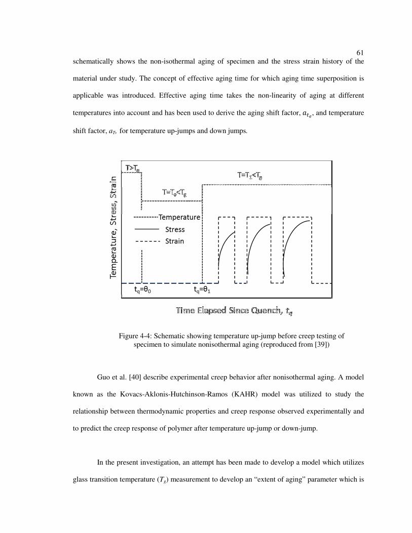
61

schematically shows the non-isothermal aging of specimen and the stress strain history of the

material under study. The concept of effective aging time for which aging time superposition is

applicable was introduced. Effective aging time takes the non-linearity of aging at different

temperatures into account and has been used to derive the aging shift factor, v��, and temperature

shift factor, aT, for temperature up-jumps and down jumps.

Guo et al. [40] describe experimental creep behavior after nonisothermal aging. A model

known as the Kovacs-Aklonis-Hutchinson-Ramos (KAHR) model was utilized to study the

relationship between thermodynamic properties and creep response observed experimentally and

to predict the creep response of polymer after temperature up-jump or down-jump.

In the present investigation, an attempt has been made to develop a model which utilizes

glass transition temperature (Tg) measurement to develop an “extent of aging” parameter which is

Figure 4-4: Schematic showing temperature up-jump before creep testing of

specimen to simulate nonisothermal aging (reproduced from [39])

62

linked to the creep response of the polymer. The novelty of this technique is in the ease with

which aging can be characterized for a complex thermal history of the polymer, which governs its

creep behavior. The advantage of using this technique over preceding work to model non-

isothermal aging is that creep response is not derived from parameters of a structural recovery

model but a more tangible experimentally measured quantity.

4.4 Experiment

4.4.1 Tensile Creep Test Specimen Preparation

To study the creep behavior of plain epoxy resin, tensile coupons of plane resin of

approximately 152.4 mm (6 inch) length, 12.7 mm (0.5 inch) width and 6.35 mm (0.25 inch)

thickness were tested under constant loading. The specimen was made by first molding 6.35 mm

(0.25 inch) thick resin sheet and then cutting it to suitable dimensions. For making the resin sheet,

MBrace

saturant resin (BASF Corporation) was mixed according to the manufacturer’s

recommendation. The resin was degassed in a vacuum chamber and then poured into a mold

(Figure 4-5). The mold was assembled over a polytetraflouroethylene (PTFE) block. An

aluminum frame was placed on the PTFE block with caulking all around the periphery. Two 6.35

mm (0.25 inch) steel rods of equal length were placed at appropriate distance inside the frame to

control the thickness of the cast sheet. A top PTFE plate rested over the steel rods to make a

closed mold assembly. The frame and steel rods were sprayed with release agent before pouring

the mixed, degassed resin.

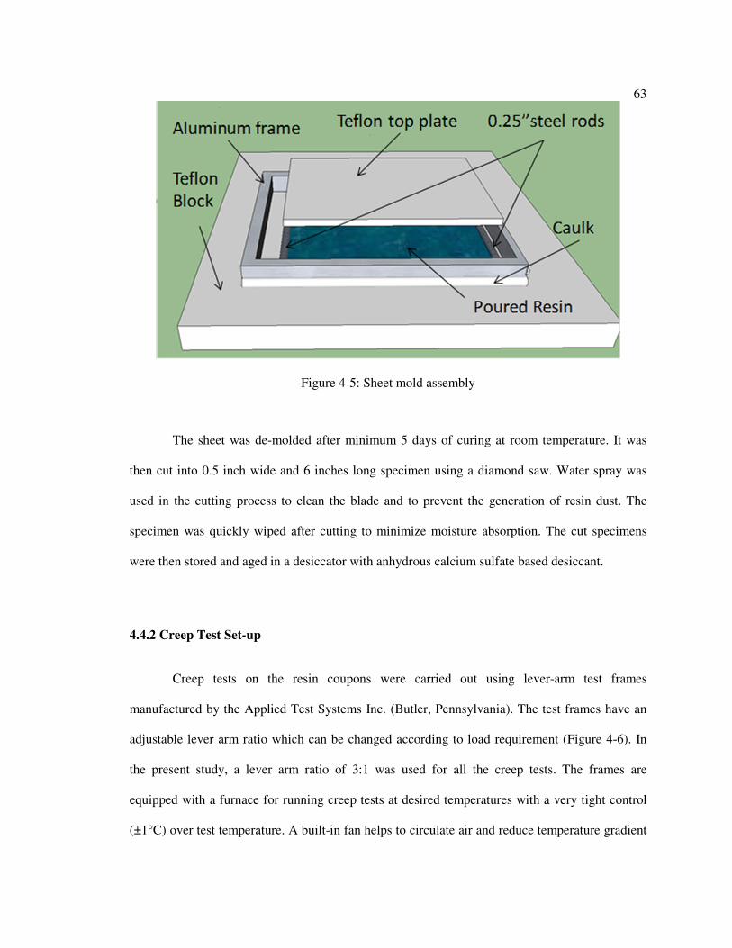
63

Figure 4-5: Sheet mold assembly

The sheet was de-molded after minimum 5 days of curing at room temperature. It was

then cut into 0.5 inch wide and 6 inches long specimen using a diamond saw. Water spray was

used in the cutting process to clean the blade and to prevent the generation of resin dust. The

specimen was quickly wiped after cutting to minimize moisture absorption. The cut specimens

were then stored and aged in a desiccator with anhydrous calcium sulfate based desiccant.

4.4.2 Creep Test Set-up

Creep tests on the resin coupons were carried out using lever-arm test frames

manufactured by the Applied Test Systems Inc. (Butler, Pennsylvania). The test frames have an

adjustable lever arm ratio which can be changed according to load requirement (Figure 4-6). In

the present study, a lever arm ratio of 3:1 was used for all the creep tests. The frames are

equipped with a furnace for running creep tests at desired temperatures with a very tight control

(±1°C) over test temperature. A built-in fan helps to circulate air and reduce temperature gradient

64

in the furnace. An external temperature controller is used to control the temperature of the creep

oven. The room temperature creep tests were done with the furnace open in a room with good

control over temperature fluctuations (22±2°C). A temperature logger was used to record the test

temperature during the creep tests. Weight plates are loaded on a motorized movable platform

which is used for slow and smooth loading and unloading of the specimen. A position sensor

attached on the lever arm triggers the vertical movement of the load train to ensure that the lever

arm remains horizontal even after considerable deformation of the specimen.

Figure 4-6: Lever arm creep frame

To minimize bending due to machine misalignment, double knife edge alignment

couplings were used in the load train. Two different types of grip were used on the two creep

65

frames. One was a modified wedge grip assembly and the other was a custom-made clamp grip

assembly (shown in Figure 4-7). Figure 4-7 also shows the extensometers mounted on opposite

faces of the specimen to measure average tensile strain and also to evaluate the bending in the

specimen. Strain gage based extensometers were preferred over strain gages mounted directly to

the specimen because polymeric resins used to attach strain gages at ambient temperature are also

susceptible to creep. The strain gages inside the extensometers are bonded using high-temperature

resins and were rated for use in temperatures exceeding the highest test temperature in the current

investigation. The extensometers used were all 0.5 inch in gage length and were manufactured by

MTS Systems Corp. (Model no. 632.31E-24) and Epsilon Technology Corp. (Model no. 3442).

During the initial setup of the load frames the machine alignment was verified by testing and

evaluating the expected strain and elastic modulus of a rectangular cross-section aluminum

coupon. During the test, specimen was loaded and the oven heat was turned on at the same time.

Elevated temperature could not be equilibrated prior to the application of load because too much

deformation was induced on the specimen by the grips and extensometers,

Average creep compliance (D) is calculated as shown in Equation 4-1, where mF and my

are the total strains measured by the two extensometers on the opposite faces of specimen and mF5

and my� are the instantaneous elastic strains measured by two extensometers.

u � z{|z}

.~+ z{�|z}�

.~ (4-1)

Instantaneous elastic strain ( mF5 and my� ) in the case of test done at 22°C was the strain

corresponding to the instant the specimen was loaded. For tests done at 30°C and 35°C, the strain

at the instant of 10 minutes into the test (after equilibrium temperature was reached) was assigned

as the instantaneous elastic strain.

66

Figure 4-7: Wedge grip assembly with extensometers mounted specimen (left) and

custom-made clamp grip assembly (right).

4.3.3 Creep Test Program

The creep test program was designed to study the effect of temperature and aging on the

creep response of plain epoxy resin. Epoxy coupons were tested at three different ages of 7, 30

and 100 days and temperatures of 22°C, 30°C and 35°C. The specimens were all aged at room

temperature—approximately 22°C. The rationale for choosing the test temperatures was to

evaluate the creep behavior at different temperatures below the Tg which are practically

achievable for structures in service. Creep tests were carried out for a duration of approximately

5000 minutes. Table 4-2 summarizes the creep test matrix.

67

Table 4-2: Number of specimens tested for each combination of age (prior to test) and

temperature during test

Temperature-22°C Temperature-30°C Temperature-35°C

Age-7 Days 3 5 3

Age-30 Days 3 3 3

Age-100 Days 3 3 3

According to the test matrix, a minimum of three specimens were tested for 9 different

testing conditions. Specimens were named as XXD-YY°C-Z where XX represents the age in

days, YY represents the test temperature in °C and Z represents the batch name. For example,

30D-35°C-1 represents a 30 days aged specimen tested at 35°C belonging to Batch 1. The

specimens tested at 22°C were tested at a stress level close to 10 MPa whereas the specimens at

30°C and 35°C were tested at stress level close to 2 MPa (except one, 100D-35°C-17, which was

tested at 10.29 MPa). The linearity of creep response with stress at higher creep temperatures was

checked by testing one particular specimen at stress level of 10.29 MPa.

Specimen 7D-22°C-2 was crept for shorter duration of time (approximately 1000

minutes). The results of this test, along with momentary creep results for specimens from the

same batch of resin at the age of 3 and 5 days, were used to study the validity of time-aging time

superposition principle and create a master curve for 7D-22°C-2 creep response. The details of

this investigation has been included in Appendix B. Table 4-3 summarizes the individual

specimen dimensions and stress levels for the creep test.

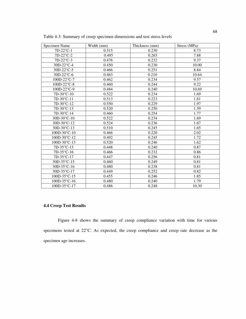
68

Table 4-3: Summary of creep specimen dimensions and test stress levels

Specimen Name Width (mm) Thickness (mm) Stress (MPa)

7D-22°C-1 0.515 0.230 8.73

7D-22°C-2 0.495 0.265 7.88

7D-22°C-3 0.476 0.232 9.37

30D-22°C-4 0.450 0.230 10.00

30D-22°C-5 0.466 0.251 8.84

30D-22°C-6 0.463 0.210 10.64

100D-22°C-7 0.462 0.234 9.57

100D-22°C-8 0.460 0.244 9.22

100D-22°C-9 0.484 0.240 10.69

7D-30°C-10 0.522 0.234 1.69

7D-30°C-11 0.513 0.223 1.81

7D-30°C-12 0.550 0.229 1.97

7D-30°C-13 0.520 0.250 1.59

7D-30°C-14 0.460 0.254 1.77

30D-30°C-10 0.522 0.234 1.69

30D-30°C-12 0.524 0.236 1.67

30D-30°C-13 0.510 0.245 1.65

100D-30°C-10 0.466 0.220 2.02

100D-30°C-12 0.492 0.245 1.72

100D-30°C-13 0.520 0.246 1.62

7D-35°C-15 0.448 0.240 0.87

7D-35°C-16 0.466 0.232 0.86

7D-35°C-17 0.447 0.256 0.81

30D-35°C-15 0.460 0.249 0.81

30D-35°C-16 0.480 0.238 0.81

30D-35°C-17 0.449 0.252 0.82

100D-35°C-15 0.455 0.246 1.85

100D-35°C-16 0.480 0.240 1.79

100D-35°C-17 0.486 0.248 10.30

4.4 Creep Test Results

Figure 4-8 shows the summary of creep compliance variation with time for various

specimens tested at 22°C. As expected, the creep compliance and creep rate decrease as the

specimen age increases.

69

Figure 4-8: Summary of creep compliance versus time at 22°C

Figures 4-9 and 4-10 show the creep test results for specimens tested at 30°C and 35°C at

different ages. Compared to 22°C creep tests, the batch scatter for 7-day-old specimens is

magnified as the test temperature is increased. The batch variability is most probably due to

variation in the curing conditions as the experimental program was spread over a year, resulting

in variation in temperature and humidity conditions under which the specimen were cured.

0 1000 2000 3000 4000 5000 6000 7000

0.0000

0.0001

0.0002

0.0003

0.0004

0.0005

0.0006

0.0007

7D-22°C-1

7D-22°C-2

7D-22°C-3

30D-22°C-4

30D-22°C-5

30D-22°C-6

100D-22°C-7

100D-22°C-8

100D-22°C-9

Cre

ep

Co

mp

liance

(1

/MP

a)

Time (Minutes)

70



0 1000 2000 3000 4000 5000 6000

0.00

0.01

0.02

0.03

7D-30°C-10

7D-30°C-11

7D-30°C-12

7D-30°C-13

7D-30°C-14

30D-30°C-10

30D-30°C-12

30D-30°C-13

100D-30°C-10

100D-30°C-12

100D-30°C-13

Cre

ep C

om

plia

nce

(1

/MP

a)

Time (Minutes)

0 1000 2000 3000 4000 5000 6000 7000

0.00

0.01

0.02

0.03

0.04

7D-35°C-15

7D-35°C-16

7D-35°C-17

30D-35°C-15

30D-35°C-16

30D-35°C-17

100D-35°C-15

100D-35°C-16

100D-35°C-17

Cre

ep C

om

plia

nce (

1/M

Pa

)

Time (Minutes)

71

A sum of exponential functions as expressed in Equation 4-2 gave a good fit to the variation of

creep compliance, D, with time (t) for individual creep tests done at 30°C and 35°C.

u � ,-Vs�� ,WVs�� (4-2)

The creep compliance of individual specimens at 22°C could be fitted using a power law in time,

as expressed in Equation 4-3.

u � �-$�� (4-3)

The experimentally obtained results from three (five in one case) different batches were averaged

out to obtain a single representative creep behavior for each test condition which is used for

comparisons and for modeling the creep behavior. The testing conditions and corresponding

representative creep functions are listed in Table 4-4.

72

Table 4-4: Average representative creep compliance functions for various test conditions Test

Condition Average Representative Function

7D-22°C

["2.009%"10+5%"t0.3885% � "1.973%"10+5%"t0.4262% � "2.441%"10+5%"t0.3899%]/3

7D-30°C

["0.01696VW.XWX"-5il%� + 0.01621V>5.55.-kT�%

�00.01034V-.-]k"-5ij%� + 0.008943V>5.55.W-]�4

�00.02766VU.X5U"-5il%� + 0.02757V>5.55.UU-�4

�"0.004397V..W5k"-5ij%� + 0.003774V>5.55-.k�%

�"0.01242VT.WSU"-5il%� + 0.01177V>5.55-X.S�%]/5

7D-35°C

["0.007038V-..5X"-5ij%� + 0.007496V>5.55..]X�%

�"0.01738VW.US-"-5il%� + 0.01951V>5.55WXXk�%

�"0.03526V..SW"-5il%� + 0.03791V>5.55UU5T�%]/3

30D-22°C

["5.234%"10+6%t0.4107 � "3.461%"10+6%t0.3894 � "1.799%"10+6%t0.5449]/3

30D-30°C

["0.001142VX.kkS"-5ij%� + 0.0005226V>5.555S-WW�%

�"0.003151VW.XU]"-5i�%� + 0.002276V>5.555UXW]�%

�"0.0009454V5.555-5].� + 0.0004154V>5.555TW-U�%]/3

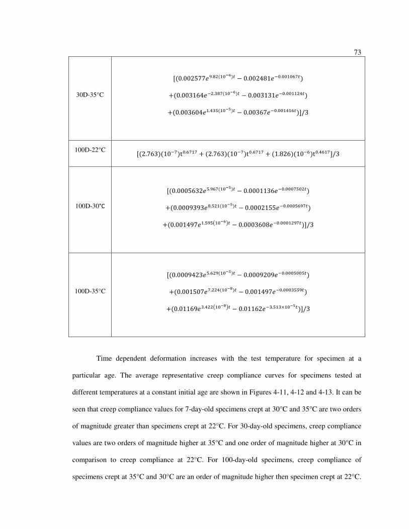
73

30D-35°C

["0.002577VS.T."-5il%� + 0.002481V>5.55-5X]�%

�"0.003164V>..WT]"-5il%� + 0.003131V>5.55--.U�%

�"0.003604V-.UWk"-5ij%� + 0.00367V>5.55-U-X�%]/3

100D-22°C

["2.763%"10>]%t5.X]-] � "2.763%"10>]%t5.X]-] � "1.826%"10>X%t5.UX-]]/3

100D-30°C

["0.0005632Vk.SX]"-5ij%� + 0.0001136V>5.555]k5.�%

�"0.0009393VT.k.-"-5ij%� + 0.0002155V>5.555kXS]�%

�"0.001497V-.kSk0-5il4� + 0.0003608V>5.555-.S]�%]/3

100D-35°C

["0.0009423Vk.X.S"-5ij%� + 0.0009209V>5.555k55k�%

�"0.001507V]...U"-5i�%� + 0.001497V>5.555WkkS�%

�"0.01169VW.U..0-5i�4� + 0.01162V>W.k-W×-5ij�%]/3

Time dependent deformation increases with the test temperature for specimen at a

particular age. The average representative creep compliance curves for specimens tested at

different temperatures at a constant initial age are shown in Figures 4-11, 4-12 and 4-13. It can be

seen that creep compliance values for 7-day-old specimens crept at 30°C and 35°C are two orders

of magnitude greater than specimens crept at 22°C. For 30-day-old specimens, creep compliance

values are two orders of magnitude higher at 35°C and one order of magnitude higher at 30°C in

comparison to creep compliance at 22°C. For 100-day-old specimens, creep compliance of

specimens crept at 35°C and 30°C are an order of magnitude higher then specimen crept at 22°C.

74

It should be noted that the specimen is evolving while it is being tested owing to physical aging

phenomena. At temperatures close to Tg, the rate of aging is high and the specimen is evolving at

a faster rate. Hence, at a particular instant of time during the creep test, a specimen at a higher

temperature would have evolved farther towards equilibrium as compared to a specimen tested at

a lower temperature.


22°C, 30°C and 35°C.

0 1000 2000 3000 4000 5000 6000

0.000

0.005

0.010

0.015

0.020

0.025

7D-22°C

7D-30°C

7D-35°C

Cre

ep

Com

plia

nce (

1/M

Pa

)

Time (Minutes)

75


22°C, 30°C and 35°C


22°C, 30°C and 35°C

As was mentioned in the description of the creep test procedure, elastic compliances were

recorded 10 minutes from the start of the creep test, once the temperature reached equilibrium.

Upon inversion of the elastic compliance, the elastic modulus is obtained. Thus, the recorded

0 1000 2000 3000 4000 5000

0.0000

0.0005

0.0010

0.0015

0.0020

0.0025

0.0030

0.0035

30D-22°C

30D-30°C

30D-35°CC

reep

Com

plia

nce (

1/M

Pa

)

Time (Minutes)

0 1000 2000 3000 4000 5000

0.0000

0.0002

0.0004

0.0006

0.0008

0.0010

0.0012

0.0014

0.0016

100D-22°C

100D-30°C

100D-35°C

Cre

ep

Com

plia

nce (

1/M

Pa

)

Time (Minutes)

76

elastic moduli may be artificially low versus true instantaneous elastic moduli. Table 4-5

summarizes the elastic modulus of epoxy resin characterized at various ages and test

temperatures. Figure 4-14 shows age-dependent functions to predict the elastic modulus of epoxy

resin at different test temperatures.

Table 4-: Elastic modulus of epoxy resin at different ages and test temperatures.

Test

condition

Trial 1

Elastic

Modulus

(MPa)

Trial 2

Elastic

Modulus

(MPa)

Trial 3

Elastic

Modulus

(MPa)

Trial 4

Elastic

Modulus

(MPa)

Trial 5

Elastic

Modulus

(MPa)

Average

Elastic

Modulus

(MPa)

Coefficient

of Variation

(%)

7D-22°C 3130 3130 3070 * * 3106 1.1

30D-22°C 3200 3200 4600 * * 3669 22

100D-

22°C 3860 3840 3990 * * 3897 2.13

7D-30°C 905 769 846 1587 1204 1062 31.68

30D-30°C 1786 1205 2222 * * 1737 29

100D-

30°C 2222 2656 2475 * * 2451 8.8

7D-35°C 719 775 971 * * 821 16

30D-35°C 1050 1110 1120 * * 1093 3.8

100D-

35°C 1430 1770 2330 * * 1841 24

77

Figure 4-14: Best-fit functions for elastic modulus of epoxy resin at various ages and

temperatures

4.5 Modeling Creep Response in Epoxy Resin

To model the creep response of the aging epoxy resin at different temperature a modified

Findley’s power law as expressed in Equation 4-4 is used.

u"$% � G"�$%tV>L/<= (4-4)

In Equation 4-4, D is the creep compliance corresponding to creep time t, A and b are the power

law parameters, Q is the creep activation energy, R is the universal gas constant (8.314 J/K/mole)

and T is temperature of creep test in Kelvin. The creep response is dependent on age of the

specimen and test temperature. The effect of age is incorporated into the model by means of the

“extent of aging” parameter (β). The parameters A and b are assumed to be functions of

0 20 40 60 80 100 1200

500

1000

1500

2000

2500

3000

3500

4000

E35°C=471.67(age)0.26178

E30°C=597.88(age)0.30756

22°C

30°C

35°C

Ela

stic M

od

ulu

s (

MP

a)

Age (Days)

E22°C=2682.97(age)0.08385

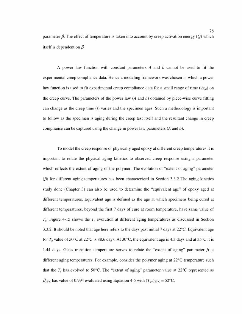
78

parameter β. The effect of temperature is taken into account by creep activation energy (Q) which

itself is dependent on β.

A power law function with constant parameters A and b cannot be used to fit the

experimental creep compliance data. Hence a modeling framework was chosen in which a power

law function is used to fit experimental creep compliance data for a small range of time (∆tfit) on

the creep curve. The parameters of the power law (A and b) obtained by piece-wise curve fitting

can change as the creep time (t) varies and the specimen ages. Such a methodology is important

to follow as the specimen is aging during the creep test itself and the resultant change in creep

compliance can be captured using the change in power law parameters (A and b).

To model the creep response of physically aged epoxy at different creep temperatures it is

important to relate the physical aging kinetics to observed creep response using a parameter

which reflects the extent of aging of the polymer. The evolution of “extent of aging” parameter

(β) for different aging temperatures has been characterized in Section 3.3.2 The aging kinetics

study done (Chapter 3) can also be used to determine the “equivalent age” of epoxy aged at

different temperatures. Equivalent age is defined as the age at which specimens being cured at

different temperatures, beyond the first 7 days of cure at room temperature, have same value of

Tg. Figure 4-15 shows the Tg evolution at different aging temperatures as discussed in Section

3.3.2. It should be noted that age here refers to the days past initial 7 days at 22°C. Equivalent age

for Tg value of 50°C at 22°C is 88.6 days. At 30°C, the equivalent age is 4.3 days and at 35°C it is

1.44 days. Glass transition temperature serves to relate the “extent of aging” parameter β at

different aging temperatures. For example, consider the polymer aging at 22°C temperature such

that the Tg has evolved to 50°C. The “extent of aging” parameter value at 22°C represented as

β22°C has value of 0.994 evaluated using Equation 4-5 with (Tg∞)22°C = 52°C.

79

β..°f � "1� � 273%/""1�B%..°f � 273% (4-5)

If this specimen is instantaneously exposed to 30°C, β30°C calculated using Equation 4-6 will have

the value 0.982, with (Tg∞)30°C = 56°C.

βW5°f � "1� � 273%/""1�B%W5°f � 273% (4-6)

In this manner, equivalent values of “extent of aging” parameter can be evaluated at different

temperatures.

Figure 4-15: Tg evolution at different aging temperatures.

The creep prediction model is trained on the average experimental result for 7D-30°C

creep compliance data. The test case 7D-30°C was chosen for training the model as it enabled

prediction of creep during up-jump (35°C) and down-jump (22°C) temperature changes based on

the available data for evaluating activation energy during aging. Also, the largest number of

experimental creep tests was run at this temperature, providing the most confidence in the time

80

dependence of deformation. Power law functions for creep compliance in the form of Equation 4-

7 are fitted to various time slices (∆tfit) as shown in Figure 4-16. Time slices (∆tfit) was selected to

be small enough to get a good fit for Equation 4-7 but large enough to keep the modeling

computationally simple.

u � G"$%t (4-7)

The variation of β30°C with aging time at 30°C is also known from results of Section 3.3.2 and has

been plotted on the same plot in Figure 4-16. The fitted parameters A and b for different ranges of

time and corresponding “extent of aging” parameter, β30°C are tabulated in Table 4-6.

Figure 4-16: Piecewise power law fitted to average representative creep compliance

curve for 7-day-old specimen tested at 30°C

0 1000 2000 3000 4000 5000 6000 7000

0.000

0.002

0.004

0.006

0.008

0.010

0.012

0.014

0.016 Experimental Average

Cre

ep

Co

mp

liance

(1

/MP

a)

Time (Minutes)

Exte

nt

of

Ag

ing P

ara

me

ter

(β3

0°C

)

0.94

0.95

0.96

0.97

0.98

0.99

1.00

∆tfit

81

Table 4-: Fitted creep law parameters A and b for different ranges of creep time and

corresponding “extent of aging” parameter at 30°C

Creep Time, t

(Minutes)

Extent of aging

parameter, β30°C

A b

0-480 0.951367-0.955097 8.21E-05 0.7583

480-840 0.955097-0.957661 0.000507 0.4601

840-1200 0.957661-0.960074 0.001606 0.2884

1200-1560 0.960074-0.962345 0.003462 0.1798

1560-1920 0.962345-0.964483 0.005604 0.1142

1920-2280 0.964483-0.966496 0.007478 0.07596

2280-2640 0.966496-0.96839 0.008548 0.0586

2640-3000 0.96839-0.970173 0.009494 0.04522

3000-3360 0.970173-0.971852 0.01002 0.03850

3360-3720 0.971852-0.973432 0.01025 0.03568

3720-4080 0.973432-0.974919 0.01029 0.03514

4080-4440 0.974919-0.976319 0.01022 0.03594

4440-4800 0.976319-0.977637 0.01009 0.03754

4800-5160 0.977637-0.978878 0.009912 0.03963

5160-5520 0.978878-0.980046 0.009712 0.04201

5520-5880 0.980046-0.981145 0.0095 0.04458

5880-6240 0.981145-0.98218 0.009281 0.04727

t > 6240 0.98218-1 0.00906 0.05003

The creep compliance prediction at 30°C, D30°C can be transformed to creep compliance

prediction at another temperature T via the creep activation energy Q, as expressed in Equation

(4-8).

u= = uW5°f (�(i`/(�(�_��))�i`/(�(��_��) ) (4-8)

82

The creep activation energy is assumed to depend on the “extent of aging” parameter and is

modeled accordingly.

To determine Q, the logarithm of the creep law (Equation 4-4) is taken.

ln(u=) = ln(G) + �ln($) − ( L<=) (4-9)

The value of (-Q/R) can be found by plotting ln(DT) against (1/T) and choosing creep compliance

values at a constant value of β from creep tests done at 7 days age at different temperatures—

i.e., 22°C, 30°C and 35°C. By choosing DT values at a constant value of β , parameters A and b

are fixed. The percentage change in the term ln(t) for the same value of β at different

temperatures is small enough to make the term [ln(A)+bln(t)] nearly constant and the variation of

ln(u=) with (1/T) a linear relation. Using creep compliance values at constant β also facilitates

the evaluation of Q as a function of β. Figure 4-17 shows an example of points picked at the same

value of β (β=0.965) at different temperatures. From these points, the values of ln(t) at

temperatures of 22°C, 30°C and 35°C are 7.4, 7.7 and 8.8, respectively. Using Table 4-6, the

values of [ln(A)+bln(t)] are -4.22,-4.31 and -4.33 at temperatures of 22°C, 30°C and 35°C,

respectively. Therefore the change in the value of [ln(A)+bln(t)] is approximately 0.1 while the

changes in ln(DT) and (Q/RT) are approximately 3, which allows the assumption that

[ln(A)+bln(t)] is a constant with varying temperature for a given value of β.

83

Figure 4-17: Creep compliance curves of 7-day-old epoxy resin tested at different temperatures

with points of β=0.965 marked

Since the Tg and resulting value of β change very slowly with time at 22°C, the 7D-22°C

representative creep compliance curve had to be extrapolated using the corresponding equation

from Table 4-4 to determine creep compliances at similar values of β as used in the higher two

temperatures. Figure 4-18 shows the plot of ln(DT) against (1/T) made by picking points at same

value of β at different temperatures, as discussed above. The figure also shows the linear

functions fitted to the three temperatures corresponding to a particular value ofβ. The slope of

each plot represents the value of Q/R corresponding to selected values ofβ.

0 2000 4000 6000 8000

0.000

0.005

0.010

0.015

0.020

0.025

7D-35°C

7D-30°C

7D-22°C

Cre

ep

Co

mp

lian

ce

(1

/MP

a)

Time (Minutes)

84

Figure 4-18: Graph for determination of activation energy at various β.

The variation of Q/R with values of “extent of aging” parameter β is shown in Figure 4-

19. A few fictitious points (encircled), with assignment based on the observed trend, were added

at very low and high values of β to cover the entire range of β observed during all the creep tests.

A power law expressed in Equation 4-10 was used to fit this data.

L< = 14826a>-U (4-10)

where the units of Q/R are Kelvin.

0.00325 0.00330 0.00335 0.00340

-8.0

-7.5

-7.0

-6.5

-6.0

-5.5

-5.0

-4.5

-4.0

-3.5

β=0.9633

β=0.965

β=0.97

β=0.972

β=0.98

β=0.9825β=0.985

ln(C

ree

p C

om

plia

nce)

1/T (Kelvin-1

)

β=0.99

85

Figure 4-19: Variation of (Q/R) with “extent of aging” parameter β

Equipped with the knowledge of evolution of β at three different temperatures, the

dependence of creep power law parameters A and b on β30°C and the transformation of creep

compliance at 30°C to creep compliance at other temperatures using the β-dependent thermal

activation energy, an attempt to model creep behavior in epoxy at different ages and creep

temperatures was made. A MATLAB

based computer code Creepmodeling (Appendix C) was

developed for this purpose. The modeling frame work has been shown in form of a flowchart in

Figure 4-20. The user inputs the creep temperature (T), aging time at 22°C (ta) and creep duration

(t). Although the initial β could be evaluated for various initial aging temperatures prior to creep,

the model is currently written for initial aging at 22°C.

0.95 0.96 0.97 0.98 0.99 1.00 1.01

15000

20000

25000

30000

35000 Power Law fit

Q/R

(K

elv

in)

Extent of Aging Parameter (β)

86

Using the methodology discussed above, before the start of a creep test, the equivalent

age at 30°C (ta30°C) and equivalent β at 30°C (βi30°C) are calculated for aging time at 22°C (ta). For

the creep duration (t), the code iteratively evaluates the “extent of aging” parameter (β30°C) based

on the aging map at 30°C and corresponding values of creep power law parameters A and b

(using Table 4-6). The evolution of β30°C starts with the initial value of βi30°C and evolves as the Tg

evolves at 30°C (Figure 4-15). The creep compliance (D30°C) at time t, for ta greater than 7 days is

calculated as expressed in Equation (4-11).

u30°�($) = G($ + $v30°�)� − G�($v30°�)�� (4-11)

where Ai and mi are values of A and m corresponding to initial value of aging parameter(β W5°f).

It can be seen that the creep compliance function depends on the instantaneous value of “extent of

aging” parameter (β30°C), initial age ($�W5°f) and “extent of aging” parameter of the material prior

to creep loading (β W5°f).

Depending upon the creep temperature (T), creep compliance at 30°C (D30°C) can be

transformed to creep compliance at temperature T (DT) using Equation 4-8. The values of β are

evaluated iteratively depending on creep temperature T using the aging map at different

temperatures from Figure 4-15. Then, the creep activation energy (Q), which depends on β, is

evaluated. Thus, the temperature-dependent time evolution in creep activation energy is evaluated

by Equation 4-10, which is in turn used in Equation 4-8 to evaluate DT.

87

Figure 4-20: Creep prediction flowchart

If ti<t

Evaluate β30°C

(t) and A(β30°C

) and m(β30°C

)

Evaluate D30°C

(t)

If T=30°C

Initialize t’=0

Plot DT vs time (t)

DT(t)= D

30°C(t)

If t’<t

Evaluate β(t’), Q(t’), and DT

Yes

Yes

No

No

No Yes

Evaluate $�W5°f and βi30°C

Input creep duration (t) in minutes

Initialize ti=0

Input aging time at 22°C (ta), creep temperature

(T) and creep duration (t)

$ = $ + 1

$′ = $′ + 1

88

The results for creep compliance prediction in epoxy specimen at age of 30 and 100

days and creep temperatures of 22°C, 30°C and 35°C have been summarized in Figures 4-21

to 4-26 along with corresponding bands of experimental scatter. The creep model predicts

the creep compliance behavior within the experimental scatter for most of the cases. The

model prediction for 30D-35°C was not realistic as a slight decrease in creep compliance

was observed in between 1000 to 3000 minutes. At greater times, however, the correct creep

compliance rate is captured.

Figure 4-21: Model prediction for creep of 30D-22°C specimen

0 1000 2000 3000 4000 5000 6000

0.00000

0.00005

0.00010

0.00015

0.00020

0.00025 Experimental Scatter

Model Prediction

Cre

ep

Co

mp

lian

ce

(1

/MP

a)

Time (Minutes)

89



0 1000 2000 3000 4000 5000 6000

0.0000

0.0005

0.0010

0.0015

0.0020


Model Prediction

Cre

ep

Co

mp

lian

ce

(1/M

Pa

)

Time (Minutes)

0 1000 2000 3000 4000 5000

0.000

0.001

0.002

0.003

0.004


Model prediction

Cre

ep C

om

plia

nce (

1/M

Pa)

Time (Minutes)

90



0 1000 2000 3000 4000 5000 6000

0.00000

0.00002

0.00004

0.00006

0.00008

0.00010


Model prediction

Cre

ep

Com

plia

nce

(1

/MP

a)

Time (Minutes)

0 1000 2000 3000 4000 5000 6000

0.0000

0.0002

0.0004

0.0006

0.0008

0.0010

Experimental Scatter

Model Prediction

Cre

ep

Com

plia

nce (

1/M

Pa

)

Time (Minutes)

91


4.6 Conclusion

Tensile creep characteristics of epoxy resin coupons were studied at the ages of 7, 30 and

100 days and creep temperatures of 22°C, 30°C and 35°C. As material aged, it became stiffer and

its creep compliance and creep rate decreased. The knowledge of physical aging kinetics was

utilized to link the mechanically observed creep behavior to a the newly proposed “extent of

aging” parameter (β). The novelty of this technique is in the ease with which aging can be

characterized for a complex thermal history of polymer which governs its creep behavior. The

advantage of using this technique over preceding techniques to model non-isothermal aging is

that creep response is not derived from parameters of a structural recovery model but a more

tangible experimentally measured quantity (glass transition temperature). A MATLAB code was

developed based on this technique to predict the creep behavior of resin aged at 22°C for a

variable time and then subjected to creep loading at different temperatures. The predictions of the

analytical model were mostly in good agreement with the experimentally observed creep behavior,

especially in capturing creep rate trends at creep times greater than 3000 minutes (50 hours).

0 1000 2000 3000 4000 5000 6000-0.0002

0.0000

0.0002

0.0004

0.0006

0.0008

0.0010

0.0012


Model Prediction

Cre

ep

Com

plia

nce (

1/M

Pa)

Time (Minutes)

92

Chapter 5 Conclusions and Recommendations for Future Work

5.1 Conclusions

The present investigation introduces a methodology for experimentally and theoretically

characterizing age- and temperature-dependent creep behavior in a representative epoxy resin that

is used for strengthening civil structures and which cures in ambient temperature conditions.

In the first phase of the investigation, the glass transition temperature (Tg) of the resin

cured and aged at 22°C was characterized using dynamic mechanical analysis (DMA) and

differential scanning calorimetry (DSC) at ages of 7, 30 and 100 days. The results showed a

dependence of Tg on the method used to assign Tg. Based on DMA scans, Tg was assigned using

the variation of storage modulus, loss modulus and Tan δ with temperature. DSC thermograms

were used to assign Tg at the onset of glass transition. The results showed a precariously low

value of Tg around 40°C at the age of 7 days which can limit the elevated temperature capability

of the structure. An increase in Tg of almost 15°C was observed between a 7-day-old resin

specimen and a specimen aged 100 days at room temperature, based on the dynamic storage

modulus.

In the second phase of the investigation, the kinetics of chemical cure and physical aging

of the selected epoxy were studied using the DSC technique. An isoconversion map to predict

evolution of degree of cure (α) was developed. This map was used to conclude that no evolution

in degree of cure (α) takes place at aging temperatures up to 70°C following 7 days of curing at

93

22°C. Further, DSC experiments established that physical aging (structural relaxation) towards

material equilibrium was the cause for the increase in Tg observed at 22°C. To systematically

study the kinetics of physical aging, resin was aged at 30°C and 35°C and the evolution of Tg with

aging time was measured. An aging map, based on evolution of Tg with age at three different

temperatures—22°C, 30°C and 35°C—was constructed for use in modeling the kinetics of

physical aging. An “extent of aging” parameter (β) was defined in terms of the easily-measured

Tg to parametrize the evolution of material toward equilibrium.

The third phase of the investigation involved experimental creep measurements and

analytical modeling of the creep behavior based on specimen age and creep conditions. Tensile

creep compliance was measured in the resin at the ages of 7, 30 and 100 days at three different

temperatures—22°C, 30°C and 35°C. Creep compliance and the creep rate decreased with

increasing age of the material. The observed mechanical creep behavior was linked to the “extent

of aging” parameter (β) developed earlier and to the creep test temperature via a creep activation

energy (Q). The analytical model was used to predict creep in resin specimen undergoing non-

isothermal aging. The modeling approach adopted was successful in capturing the evolution in

material behavior during the creep test. The modeling results were in good agreement with

experimental results for most of the experimental test cases, particularly in capturing the creep

rate beyond 50 hours.

5.1 Recommendations and Scope for Future Work

− One of the keys to consistent material behavior of ambient temperature cured resin is to

maintain very tight control over temperature and humidity during molding and aging of

94

the resin. The scatter in the experimental creep results can be reduced if a climate control

chamber is used.

− Owing to time constraints, the development of the aging map was based on DSC scans on

only one batch of resin. DSC scans on multiple batches of resin following the same test

procedure will make the aging map more reliable and possibly improve the results of

creep prediction model.

− Creep behavior was assumed to be linear in stress in the modeling effort. This

assumption should be checked by running additional experiments at different stress

levels.

− The shear creep in fiber-reinforced composite laminates should also be investigated. This

type of creep could be an important contributor to the total creep deformation of a

structure strengthened with FRP laminate.

− There is a need to develop an ambient temperature cured resin system with improved

elevated temperature behavior—i.e., high Tg and low creep rate at elevated temperature.

Nanoscale reinforcements such as nanosilica, polyhedral oligomeric silsesqiuoxanes

(POSS), carbon nanofibers and nanotubes may be used to enhance the Tg and mechanical

properties at elevated temperatures.

95

− The civil infrastructure design guidelines for repair and strengthening using FRP

externally bonded reinforcements (such as ACI 440-2R-08 [12] and fib Bulletin 14 [6])

need to be amended in terms of guidelines for characterizing the Tg of the employed

resins and the elevated temperature capability of strengthened structures. There is a need

to define a standard test method for assigning Tg with specific details on curing

conditions of the resin and test parameters, as the Tg assigned is highly dependent on

them. Research is needed to characterize the residual strength of structures strengthened

with FRP and subjected to various sustained loads and various elevated temperatures.

Based on these amendments and research findings, improved guidelines for the safe

design of strengthened structures can be realized.

− The effect of humidity on the aging kinetics of epoxy resin and creep behavior of epoxy

resin should be studied and modeled. Design guidelines for structures subjected to wet

conditions should reflect these findings.

96

References

[1] Bank L.C. (2006), Composites for Construction: Structural Design with FRP Materials, 1st

edition, John Wiley & Sons Inc.

[2] Teng J.G., Chen J.F., Smith S.T., and Lam L. (2002), FRP Strengthened RC Structures, 1st

edition, John Wiley & Sons Inc.

[3] Bakis C.E., Bank L.C., Brown V.L., Cosenza E., Davalos J.F., Lesko J.J., Machida A.,

Rizkalla S.H., and Triantafillou T.C. (2002), Fiber-Reinforced Polymer Composites for

Construction—State-of-the-Art Review, Journal of Composites for Construction, Vol. 6,

pp.73-87.

[4] Matana M., Nanni A., Dharani L., Silva P., and Tunis G. (2005), Bond Performance of Steel

Reinforced Polymer and Steel Reinforced Grout, Proc. International Symposium on Bond

Behaviour of FRP in Structures (BBFS 2005), International Inst. for FRP in Construction,

pp.125-132.

[5] Huang X., Birman V., Nanni A., and Tunis G. (2003), Properties and Potential for

Application of Steel Reinforced Polymer and Steel Reinforced Grout Composites,

Composites Part B: Engineering, pp. 73-82.

[6] CEB-FIB fib Bulletin 14 (2001), Externally Bonded FRP Reinforcement for RC Structures,

International Federation for Structural Concrete (fib), Lausanne, Switzerland, 130 p.

[7] Kroschwitz J.L. (1987), Polymers: An Encyclopedic Sourcebook of Engineering Properties,

1st edition, John Wiley & Sons Inc.

[8] Chin J., Forster A. ,Ocel J., Hartmann J., Fuchs

P., and Hunston D. (2010),

Thermoviscoelastic Analysis and Creep Testing of Ambient Temperature Cure Epoxies Used

in Adhesive Anchor Applications, Journal of Materials in Civil Engineering, Vol. 22, pp.

1039-1046

[9] Bakis C.E. (2008), Elevated Temperature Capability of Epoxy Resins: Issues and

Developments, Proc. US-South America Workshop on Innovative Materials for Civil

Infrastructure, Research and Education, M.M. Lopez, Ed., National Science Foundation, 13-

15 Oct. 2008, Chile, 4 p. (CDROM).

[10] Leone M., Matthys S., and Aiello M.A. (2008), Effect of Elevated Temperature on Bond

Between FRP EBR Systems and Concrete, Composites: Part B, Vol. 40, pp. 85-93.

97

[11] Klamer E. L., Hordijk D. A., and Hermes M.C.J. (2008), The Influence of Temperature on

RC Beams Strengthened with Externally Bonded CFRP Reinforcement, HERON, pp. 157-

185.

[12] ACI Committee 440 (2008), Guide for the Design and Construction of Externally Bonded

FRP Systems for Strengthening Concrete Structures, ACI 440.2R-08, American Concrete

Institute, Farmington Hills, MI, 76 p.

[13] ASTM Standard E1640 (2004), Standard Test Method for Assignment of the Glass

Transition Temperature by Dynamic Mechanical Analysis, ASTM International, West

Conshohocken, PA.

[14] Höhne G.W.H., Hemminger W.F., and Flammersheim H.J., Differential Scanning

Calorimetry, 2nd

edition, Springer (2003).

[15] ASTM Standard D3418 (2010), Standard Test Method for Transition Temperatures and

Enthalpies of Fusion and Crystallization of Polymers by Differential Scanning Calorimetry,

Annual Book of ASTM Standards, ASTM International.

[16] Chartoff R.P., Weissman P.T., and Sircar A. (1994), The Application of Dynamic

Mechanical Methods to Tg Determination in Polymers: An Overview, Assignment of the

Glass Transition, ASTM STP 1249, R.J. Seyler, Ed., American Society for Testing and

Materials, Philadelphia, pp. 88-107.

[17] Wu L., Hoa S.V., and Ton-That M. (2004), Effects of Water on the Curing and Properties of

Epoxy Adhesive used for Bonding FRP Composite Sheet to Concrete, Journal of Applied

Polymer Science, Vol. 92, pp. 2261–2268

[18] Yang Q., Xian G., and Karbhari V. (2008), Hygrothermal Ageing of an Epoxy Adhesive

used in FRP Strengthening of Concrete, Journal of Applied Polymer Science, Vol.107, pp.

2607-2617.

[19] Zhang D., Jia D., and Chen S. (2009), Kinetics of Curing and Thermal Degradation of

Hyperbranched Epoxy (HDTE)/Diglycidyl Ether of Bisphenol-A Epoxy Hybrid Resin,

Journal of Thermal Analysis and Calorimetry, Vol. 98, pp. 819-824.

[20] Yoo M.J., Kim S.H., Park S.D., Lee W.S., Sun J., Choi J., and Nahm S. (2009),

Investigation of Cure Kinetics of Various Cycloaliphatic Epoxy Resins using Dynamic

Thermal Analysis, European Polymer Journal, Vol. 46, pp. 1158-1162.

[21] Liang G., and Chandrashekhara K. (2006), Cure Kinetics and Rheology Characterization of

Soy Based Epoxy Resin System, Journal of Applied Polymer Science, Vol. 102, pp. 3168-

3180.

98

[22] Ghaemy M., Rostami A.A., and Omrani A. (2006), Isothermal Cure Kinetics and

Thermodynamics of an Epoxy-Nickel-Diamine system, Polymer International, Vol. 55, pp.

279-284.

[23] Ruiz E. and Billotte C. (2009), Predicting the Cure of Thermosetting Polymers: The

Isoconversion Map, Polymer Composites, Vol. 30, pp. 1450-1457.

[24] Struik L.C.E. (1977), Physical Aging in Plastics and Other Glassy Materials, Polymer

Science and Engineering, Vol. 17, No. 3, pp. 165-173.

[25] Hodge I.M. (1995), Physical Aging in Polymer Glasses, Science, Vol. 267, No. 5206, pp.

1945-1947.

[26] Hutchinson J.M. (1995), Physical Aging of Polymers, Progress in Polymer Science, Vol. 20,

No. 4, pp. 703-760.

[27] Tool A.Q. (1946), Viscosity and the Extraordinary Heat Effects in Glass, Journal of

Research of the National Bureau of Standards, Vol. 37, pp. 73-90.

[28] Montserrat S. (1994), Physical Aging Studies in Epoxy Resins. Kinetics of the Enthalpy

Relaxation Process in a Fully Cured Epoxy Resin, Journal of Polymer Science, Part B:

Polymer Physics, Vol. 32, pp. 509-522.

[29] Larmagnac J.P., Grenet J., and Michon P. (1981), Glass Transition Temperature

Dependence on Heating Rate and on Ageing for Amorphous Selenium Films, Journal of

Non-Crystalline Solids, Vol. 45, Issue 2, pp. 157-168.

[30] Plazek D.J. and Frund Z.N. (1990), Epoxy Resin (DGEBA): The Curing and Physical

Aging Process, Journal of Polymer Science: Part B:Polymer Physics, Vol. 28, pp. 431-448.

[31] Moynihan C.T., Easteal A.J., DeBolt M.A., and Tucker J. (1976), Dependence of the Fictive

Temperature of Glass on Cooling Rate, Journal of the American Ceramic Society, Vol. 59,

pp. 12-16.

[32] Betten J. (2002), Creep Mechanics, Springer.

[33] Lakes R. (2009), Viscoelastic Materials, Cambridge University Press.

[34] Majda P. and Skrodzewicz J. (2009), A Modified Creep Model of Epoxy Adhesive at

Ambient Temperature, International Journal of Adhesion and Adhesives, Vol. 29, pp. 396-

404.

99

[35] Plaseied A. and Fatemi A. (2009), Tensile Creep and Deformation Modeling of Vinyl Ester

Polymer and its Nanocomposite, Journal of Reinforced Plastics and Composites, Vol. 28,

pp.1775-1788.

[36] Bakis C.E. and Temple-Boyer C.F. (2003), Tensile Creep Behavior of Carbon Nanotube

Reinforced Epoxy, Proc. 14th International Conference on Composite Materials, Society for

Manufacturing Engineers, Paper No. 2019 (CD ROM).

[37] Barbero E.J. and Ford K.J. (2004), Equivalent Time Temperature Model for Physical Aging

and Temperature Effects on Polymer Creep and Relaxation, Journal of Engineering

Material and Technology, Vol. 126, pp. 413-419.

[38] Beckmann J. and McKenna G.B. (1997), Physical Aging Kinetics of Syndiotactic

Polystyrene as Determined from Creep Behavior, Polymer Engineering and Science, Vol.

37, pp. 1459-146.

[39] Bradshaw R.D. and Brinson L.C. (1997), Recovering Nonisothermal Physical Aging Shift

Factors via Continuous Test Data: Theory and Experimental Results, Journal of Engineering

Materials and Technology, Vol. 119, pp. 233-241.

[40] Guo Y., Wang N., Bradshaw R.D., and Brinson L.C. (2008), Modeling Mechanical Aging

Shift Factors in Glassy Polymers during Nonisothermal Physical Aging.I. Experiments and

KAHR-ate model prediction, Journal of Polymer Science: Part B: Polymer Physics, Vol. 47,

pp. 340-352.

[41] Dean G. (2006), Modelling Non-Linear Creep Behavior in an Epoxy Adhesive,

International Journal of Adhesion and Adhesives, Vol. 27, pp. 636-646.

100

Appendix A

Detailed Experimental Results

DMA Results: 7-Day-Old-Storage Modulus

7A: Storage Modulus vs. Temperature

7B: Storage Modulus vs. Temperature

7C: Storage Modulus vs. Temperature

-60 -40 -20 0 20 40 60 80 100 120 140

0.0

0.5

1.0

1.5

2.0

2.5

3.0

3.5

4.0

4.5

TgR3=65 °C

TgR2=58°C

Run 1

Run 2

Run 3

Sto

rage

Modu

lus (

GP

a)

Temperature (°C)

TgR1=47°C

-50 -30 -10 10 30 50 70 90 110 130

0

1

2

3

4

5

TgR3=59°C

Run 1

Run 2

Run 3

TgR2=50°C

Sto

rage

Mo

dulu

s (

GP

a)

Temperature (°C)

TgR1=43°C

-60 -40 -20 0 20 40 60 80 100 120 140

0.0

0.5

1.0

1.5

2.0

2.5

3.0

3.5

Run 1

Run 2

Run 3

Run 4

Run 5

Run 6

TgR6=65°C

TgR5=65°C

TgR4=58°C

TgR2=46°C

TgR3=57°C

Sto

rage M

odulu

s (

GP

a)

Temperature (°C)

TgR1=36°C

101

DMA Results: 7-Day-Old-Loss Modulus

7A: Loss Modulus vs. Temperature

7B: Loss Modulus vs. Temperature

7C: Loss Modulus vs. Temperature

-60 -40 -20 0 20 40 60 80 100 120 140

0.00

0.05

0.10

0.15

0.20

0.25

0.30

0.35

0.40 TgR3=75°C

TgR2=67°C

Run 1

Run 2

Run 3

Loss M

odulu

s (

GP

a)

Temperature (°C)

TgR1=50°C

-50 -30 -10 10 30 50 70 90 110 130

0.00

0.05

0.10

0.15

0.20

0.25

0.30

0.35

0.40

0.45 Run 1

Run 2

Run 3 TgR3=76°C

TgR2=67°C

Lo

ss M

od

ulu

s (

GP

a)

Temperature (°C)

TgR1=49°C

-60 -40 -20 0 20 40 60 80 100 120 140

0.00

0.05

0.10

0.15

0.20

0.25

0.30

0.35

TgR6=80°C

TgR5=79°C

TgR4=78°CTgR3=74°C

TgR2=66°C

TgR1=44°C

Loss M

odulu

s (

GP

a)

Temperature (°C)

Run 1

Run 2

Run 3

Run 4

Run 5

Run 6

102

DMA Results: 7-Day-Old-Tan δδδδ

7A: Tan δ vs. Temperature

7B: Tan δ vs. Temperature

7C: Tan δ vs. Temperature

-60 -40 -20 0 20 40 60 80 100 120 140

0.0

0.2

0.4

0.6

0.8

1.0

1.2

1.4

1.6

1.8TgR1=59°C

TgR3=82°C

TR2=75°C

Run 1

Run 2

Run 3

Tan

δ

Temperature (°C)-40 -20 0 20 40 60 80 100 120 140

0.0

0.2

0.4

0.6

0.8

1.0

1.2

1.4

1.6 Run 1

Run 2

Run 3

TgR3=92°C

TgR2=85°C

Ta

n δ

Temperature (°C)

TgR1=60°C

-60 -40 -20 0 20 40 60 80 100 120 140

0.0

0.2

0.4

0.6

0.8

1.0

1.2

1.4

1.6

1.8 Run 1

Run 2

Run 3

Run 4

Run 5

Run 6

TgR6=95°C

TgR5=94°C

TgR4=93°C


TgR1=57°C

Tan δ

Temperature (°C)

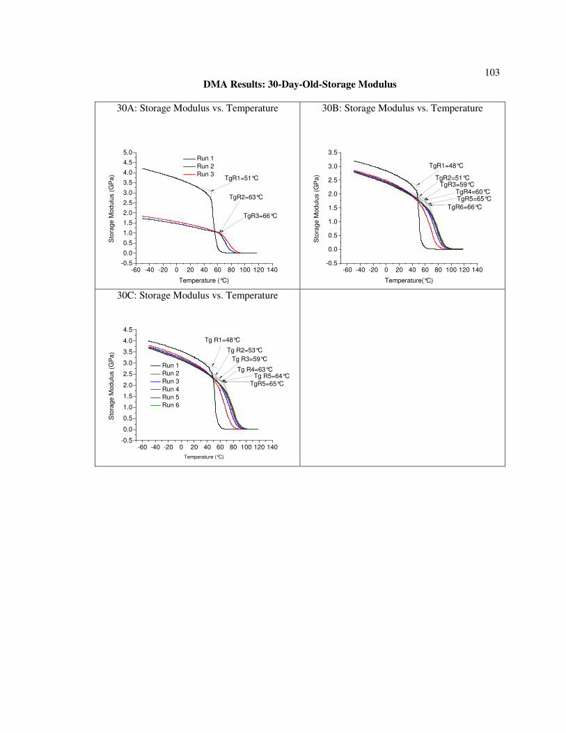
103

DMA Results: 30-Day-Old-Storage Modulus

30A: Storage Modulus vs. Temperature 30B: Storage Modulus vs. Temperature

30C: Storage Modulus vs. Temperature

-60 -40 -20 0 20 40 60 80 100 120 140-0.5

0.0

0.5

1.0

1.5

2.0

2.5

3.0

3.5

4.0

4.5

5.0 Run 1

Run 2

Run 3

TgR3=66°C

TgR2=63°C

Sto

rage M

od

ulu

s (

GP

a)

Temperature (°C)

TgR1=51°C

-60 -40 -20 0 20 40 60 80 100 120 140-0.5

0.0

0.5

1.0

1.5

2.0

2.5

3.0

3.5

TgR6=66°C



Sto

rage M

od

ulu

s (

GP

a)

Temperature(°C)

TgR1=48°C

-60 -40 -20 0 20 40 60 80 100 120 140-0.5

0.0

0.5

1.0

1.5

2.0

2.5

3.0

3.5

4.0

4.5

Run 1

Run 2

Run 3

Run 4

Run 5

Run 6

TgR5=65°CTg R5=64°C

Tg R4=63°C

Tg R3=59°C

Tg R2=53°C

Sto

rage M

od

ulu

s (

GP

a)

Temperature (°C)

Tg R1=48°C

104

DMA Results: 30-Day-Old-Loss Modulus

30A: Loss Modulus vs. Temperature 30B: Loss Modulus vs. Temperature

30C: Loss Modulus vs. Temperature

-60 -40 -20 0 20 40 60 80 100 120 140-0.05

0.00

0.05

0.10

0.15

0.20

0.25

0.30

0.35

0.40

0.45

Run 1

Run 2

Run 3

TgRun3=77°C

TgRun2=71°C

Loss M

odulu

s (

GP

a)

Temperature(°C)

TgRun1=56°C

-60 -40 -20 0 20 40 60 80 100 120 140

0.00

0.05

0.10

0.15

0.20

0.25

0.30

0.35


TgR3=75°C

TgR2=69°C

TgR6=81°C

Loss M

odu

lus (

GP

a)

Temperature (°C)

TgR1=51°C

-60 -40 -20 0 20 40 60 80 100 120 140

0.00

0.05

0.10

0.15

0.20

0.25

0.30

0.35

Run 1

Run 2

Run 3

Run 4

Run 5

Run 6

TgR6=80°C



Loss m

odu

lus (

GP

a)

Temperature (°C)

TgR1=53°C

105

DMA Results: 30-Day-Old-Tan δδδδ

30A: Tan δ vs. Temperature

30B: Tan δ vs. Temperature


-60 -40 -20 0 20 40 60 80 100 120 140

0.0

0.2

0.4

0.6

0.8

1.0

1.2

1.4

Run 1

Run 2

Run 3

TgR3=92°C

TgR2=85°C

TgR1=65°C

Tan δ

Temperature (°C)

-40 -20 0 20 40 60 80 100 120 140

0.0

0.2

0.4

0.6

0.8

1.0

1.2

1.4

1.6

Run1

Run 2

Run 3

Run 4

Run 5

Run 6TgR6=95°C

TgR5=95°C

TgR4=94°C

TgR3=92°C

TgR2=86°C

Tan

δ

Temperature (°C)

TgR1=63°C

-60 -40 -20 0 20 40 60 80 100 120 140

0.00.10.20.30.40.50.60.70.80.91.01.11.21.31.4

Run 1

Run 2

Run 3

Run 4

Run 5

Run 6R6Tg=95°C

R5Tg=95°C

R4Tg=93°CR3Tg=91°C

Run2Tg=85°C

Tan

δ

Temperature(°C)

R1Tg=64°C

106

DMA Results: 100/130-Day-Old-Storage Modulus


100B: Storage Modulus vs. Temperature


-60 -40 -20 0 20 40 60 80 100 120 140-0.5

0.0

0.5

1.0

1.5

2.0

2.5

3.0

3.5

TgR5=67°C


TgR2=57°C

Run 1

Run 2

Run 3

Run 4

Run 5

Run 6

Sto

rage M

odulu

s (

GP

a)

Temperature (°C)

TgR1=59°C

-60 -40 -20 0 20 40 60 80 100 120 140-0.5

0.0

0.5

1.0

1.5

2.0

2.5

3.0

3.5

4.0

Run 1

Run 2

Run 3

Run 4

Run 5

Run 6

Tg R6=66°C

Tg R5=65°C

Tg R4=64°C

Tg R3=60°C

Tg R2=55°C

Sto

rage M

odulu

s (

MP

a)

Temperature (°C)

Tg R1=52°C

-60 -40 -20 0 20 40 60 80 100 120 140

0.0

0.5

1.0

1.5

2.0

2.5

3.0

3.5

TgR6=66°C

TgR5=65°C

TgR4=63°C


Sto

rag

e M

od

ulu

s (

GP

a)

Temperature (°C)

TgR1=50°C

107

DMA Results: 100/130-Day-Old-Loss Modulus

100A: Loss Modulus vs. Temperature 100B: Loss Modulus vs. Temperature

130A: Loss Modulus vs. Temperature

-60 -40 -20 0 20 40 60 80 100 120 140

0.00

0.05

0.10

0.15

0.20

0.25

0.30

TgR6=82°C

TgR5=81°C


TgR2=72°C

Loss M

odulu

s (

GP

a)

Temperature (°C)

TgR1=64°C

-60 -40 -20 0 20 40 60 80 100 120 140-0.05

0.00

0.05

0.10

0.15

0.20

0.25

0.30

0.35 Run 1

Run 2

Run 3

Run 4

Run 5

Run 6

Tg Run5=81°C

Tg Run4=78°CTg Run4=80°C

Tg Run3=76°CTg Run2=70°C

Loss M

odulu

s (

MP

a)

Temperature (°C)

Tg R1=56°C

-60 -40 -20 0 20 40 60 80 100 120 140

0.00

0.05

0.10

0.15

0.20

0.25

0.30

0.35


TgR5=79°C

TgR2=70°C

TgR6=80°C

Lo

ss M

odu

lus (

GP

a)

Temperature (°C)

TgR1=56°C

108

DMA Results: 100/130-Day-Old-Tan δδδδ

100A: Tan δ vs. Temperature 100B: Tan δ vs. Temperature


-60 -40 -20 0 20 40 60 80 100 120 140

0.0

0.2

0.4

0.6

0.8

1.0

1.2

TgR6=97°C

TgR5=96°C

TgR4=95°C

TgR1=73°C

TgR3=93°C

Run 1

Run 2

Run 3

Run 4

Run 5

Run 6Tan

δ

Temperature (°C)

TgR2=88°C

-60 -40 -20 0 20 40 60 80 100 120 140

0.0

0.2

0.4

0.6

0.8

1.0

1.2

1.4

Run 1

Run 2

Run 3

Run 4

Run 5

Run 6

TgR6=94°C

TgR5=94°C

TgR4=93°C

TgR3=91°C

TgR2=85°C

Tan

δ

Temperature (°C)

TgRun1=66°C

-60 -40 -20 0 20 40 60 80 100 120 140

0.0

0.2

0.4

0.6

0.8

1.0

1.2

TgRun6=95°CTgRun5=95°CTgRun4=94°C

TgRun3=92°C

Tan

δ

Temperature (°C)

TgRun1=67°C

TgRun2=85°C

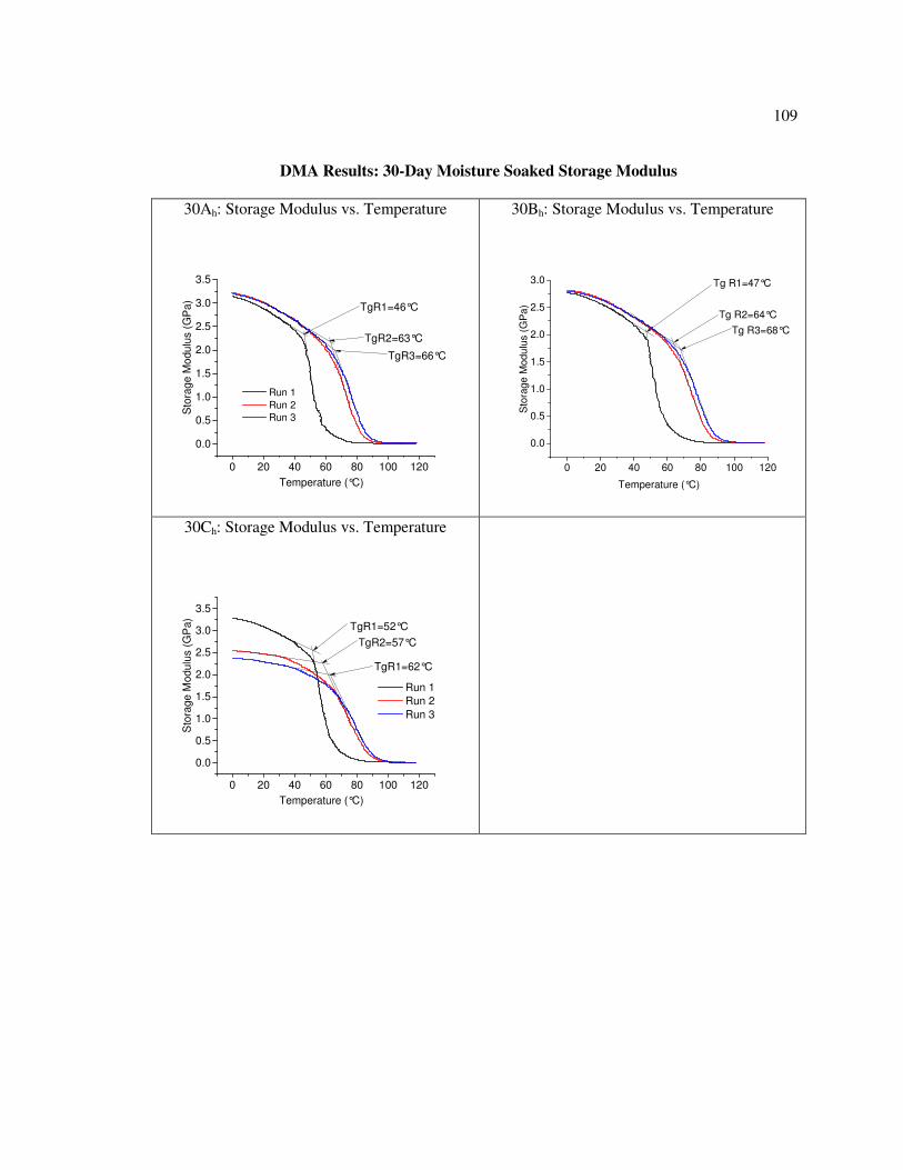
109

DMA Results: 30-Day Moisture Soaked Storage Modulus

30Ah: Storage Modulus vs. Temperature 30Bh: Storage Modulus vs. Temperature

30Ch: Storage Modulus vs. Temperature

0 20 40 60 80 100 120

0.0

0.5

1.0

1.5

2.0

2.5

3.0

3.5

Run 1

Run 2

Run 3

TgR3=66°C

TgR2=63°C

Sto

rage M

odulu

s (

GP

a)

Temperature (°C)

TgR1=46°C

0 20 40 60 80 100 120

0.0

0.5

1.0

1.5

2.0

2.5

3.0

Tg R3=68°C

Tg R2=64°C

Sto

rage M

odu

lus (

GP

a)

Temperature (°C)

Tg R1=47°C

0 20 40 60 80 100 120

0.0

0.5

1.0

1.5

2.0

2.5

3.0

3.5

TgR2=57°C

TgR1=62°C

Run 1

Run 2

Run 3

Sto

rage M

odulu

s (

GP

a)

Temperature (°C)

TgR1=52°C

110

DMA Results: 30-Day Moisture Soaked Loss Modulus

30Ah: Loss Modulus vs. Temperature

30Bh: Loss Modulus vs. Temperature

30Ch: Loss Modulus vs. Temperature

0 20 40 60 80 100 120 140

0.00

0.05

0.10

0.15

0.20

0.25

0.30

0.35

Run 1

Run 2

Run 3

TgR3=75°C

TgR2=72°C

Lo

ss M

od

ulu

s (

GP

a)

Temperature (°C)

TgR1=52°C

0 20 40 60 80 100 120

0.00

0.05

0.10

0.15

0.20

0.25

0.30

0.35

Tg R3=79°C

Tg R2=76°C

Lo

ss M

od

ulu

s (

GP

a)

Temperature(°C)

Tg R1=53°C

0 20 40 60 80 100 120

0.00

0.05

0.10

0.15

0.20

0.25

0.30

TgR3=81°C

TgR2=78°C

Run1

Run 2

Run 3

Loss M

odulu

s (

GP

a)

Temperature (°C)

TgR1=59°C

111

DMA Results: 30-Day Moisture Soaked Tan δδδδ

30Ah: Tan δ vs. Temperature 30Bh: Tan δ vs. Temperature

30Ch: Tan δ vs. Temperature

0 20 40 60 80 100 120

0.0

0.1

0.2

0.3

0.4

0.5

0.6

0.7

0.8

0.9

1.0

Run 1

Run 2

Run 3

TgR3=93°C

TgR2=89°C

Tan δ

Temperature (°C)

TgR1=77°C

0 20 40 60 80 100 120

0.0

0.1

0.2

0.3

0.4

0.5

0.6

0.7

0.8

0.9

1.0Tg R3=93°C

Tg R2=91°C

Ta

n δ

Temperature (°C)

Tg R1=78°C

0 20 40 60 80 100 120

0.0

0.2

0.4

0.6

0.8

1.0

1.2

TgR3=96°C

TgR2=94°C

Run 1

Run 2

Run 3

Ta

n δ

Temperature (°C)

TgR1=85°C

112

DMA Results: 100-Day Moisture Soaked Storage Modulus

100Ah: Storage Modulus vs. Temperature

100Bh: Storage Modulus vs. Temperature

100Ch: Storage Modulus vs. Temperature

-40 -20 0 20 40 60 80 100 120-0.5

0.0

0.5

1.0

1.5

2.0

2.5

3.0

3.5

TgR3=67°C

TgR2=64°C

Run 1

Run 2

Run 3Sto

rag

e M

od

ulu

s (

GP

a)

Temperature (°C)

TgR1=49°C

-20 0 20 40 60 80 100 120-0.5

0.0

0.5

1.0

1.5

2.0

2.5

3.0

3.5

4.0

4.5

Run 1

Run 2

Run 3

TgR2=62°C

TgR3=65°C

Sto

rag

e M

od

ulu

s (

GP

a)

Temperature(°C)

TgR1=51°C

-40 -20 0 20 40 60 80 100 120-0.5

0.0

0.5

1.0

1.5

2.0

2.5

3.0

3.5

4.0

Run 1

Run 2

Run 3

TgR3=63°C

TgR2=60°C

Sto

rag

e M

odu

lus (

Gp

a)

Temperature (°C)

TgR1=49°C

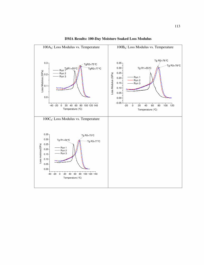
113

DMA Results: 100-Day Moisture Soaked Loss Modulus

100Ah: Loss Modulus vs. Temperature 100Bh: Loss Modulus vs. Temperature

100Ch: Loss Modulus vs. Temperature

-40 -20 0 20 40 60 80 100 120 140

0.0

0.1

0.2

0.3

TgR2=77°C Run 1

Run 2

Run 3

Lo

ss M

od

ulu

s (

GP

a)

Temperature (°C)

TgR1=55°C

TgR2=75°C

-20 0 20 40 60 80 100 120-0.05

0.00

0.05

0.10

0.15

0.20

0.25

0.30

0.35

Run 1

Run 2

Run 3

Tg R3=78°C

Tg R2=76°C

Lo

ss M

od

ulu

s (

GP

a)

Temperature (°C)

Tg R1=55°C

-40 -20 0 20 40 60 80 100 120 140

0.00

0.05

0.10

0.15

0.20

0.25

0.30

0.35

Run 1

Run 2

Run 3

Tg R3=77°C

Tg R2=75°C

Lo

ss m

od

ulu

s(G

Pa

)

Temperature (°C)

Tg R1=54°C

114

DMA Results: 100-Day Moisture Soaked Tan δδδδ

100Ah: Tan δ vs. Temperature 100Bh: Tan δ vs. Temperature

100Ch: Tan δ vs. Temperature

-40 -20 0 20 40 60 80 100 120

0.0

0.1

0.2

0.3

0.4

0.5

0.6

0.7

0.8

0.9

1.0

TgR3=91°C

TgR2=89°C

Run 1

Run 2

Run 3

Ta

n δ

Temperature (°C)

TgR1=81°C

-20 0 20 40 60 80 100 120

0.0

0.1

0.2

0.3

0.4

0.5

0.6

0.7

0.8

0.9

1.0

Run 1

Run 2

Run 3

TgR3=93°C

TgR2=90°C

Ta

n δ

Temperature (°C)

TgR1=82°C

-40 -20 0 20 40 60 80 100 120 140

0.0

0.1

0.2

0.3

0.4

0.5

0.6

0.7

0.8

0.9

1.0

Run 1

Run 2

Run 3

TgR3=91°C

TgR2=88°C

Tan

δ

Temperature (°C)

TgR1=80°C

115

DSC Results: 7-Day-Old

DSC scan 7A’

DSC scan 7B’

DSC scan 7C’

0 50 100 150 200 250

-2

-1

0

1

2

3

4

Tg' Run1=58oC

TgRun2=65oC

Hea

t F

low

(m

W)

Temperature (oC)

TgRun1=40oC

Tg' Run2=61oC

0 50 100 150 200 250

-2

-1

0

1

2

3

4

Run 2

TgRun2'=63°C

TgRun2=69°C

TgRun1'=55°C

Hea

t F

low

(m

W)

Temperature (°C)

TgRun1=40.8°C

Exo U

p

Run 1

-20 0 20 40 60 80 100 120 140 160 180

0.0

0.2

0.4

0.6

0.8

1.0

1.2

1.4

1.6

1.8

He

at

Flo

w (

mW

)

Temperature (°C)

TgRun1=40.03°C

Exo

Up

116


DSC scan 30A’

DSC scan 30B’

DSC scan 30C’

-25 0 25 50 75 100 125 150 175 200 225 250 275

-2.0

-1.5

-1.0

-0.5

0.0

0.5

1.0

1.5

2.0

2.5

3.0

3.5

TgRun2'=64οC

TgRun2=68οCH

eat F

low

(m

W)

Temperature (οC)

TgRun1=48οC

TgRun1'=58οC

0 40 80 120 160 200

-1.0

-0.5

0.0

0.5

1.0

He

at

Flo

w (

mW

)

Temperature (°C)

Tg=45.3°C

Exo

Up

0 50 100 150 200 250-1.5

-1.0

-0.5

0.0

0.5

1.0

1.5

2.0

2.5

Tg'Run1=58°C

Tg'Run2=61°C

TgRun2=66°CHe

at

Flo

w (

mW

)

Temperature (°C)

TgRun1=45.2°C

Exo U

p

117


DSC scan 100A’ DSC scan 100B’

DSC scan 100 C’

0 50 100 150 200

-1.5

-1.0

-0.5

0.0

0.5

1.0

1.5

He

at

Flo

w (

mW

)

Temperature (°C)

TgRun1=51.5°C

Exo

Up

0 50 100 150 200

-1.5

-1.0

-0.5

0.0

0.5

1.0

Hea

t F

low

(m

W)

Temperature (°C)

Exo u

p

TgRun1=56°C

0 20 40 60 80 100 120 140 160

-2.0

-1.5

-1.0

-0.5

0.0

0.5

1.0

1.5

He

at F

low

(mW

)

Temperature (°C)

Exo U

p

Tg Run1=51°C

118

Creep Test: 7D-35°C

7D-35°C-15

7D-35°C-16

7D-35°C-17

0 2000 4000 6000 80000.000

0.001

0.002

0.003

0.004

0.005

0.006

0.007

0.008

0.009

Strain A

Strain B

Average

Str

ain

Time (Minutes)

0 2000 4000 6000 8000

0.000

0.005

0.010

0.015

0.020

Strain A

Strain B

Average Strain

Str

ain

Time (Minutes)

0 1000 2000 3000 4000 5000

0.000

0.005

0.010

0.015

0.020

0.025

0.030

0.035

0.040

Strain A

Strain B

Average

Str

ain

Time (Minutes)

119


30D-35°C-15

30D-35°C-16

30D-35°C-17

0 1000 2000 3000 4000 5000

0.0000

0.0005

0.0010

0.0015

0.0020

0.0025

0.0030

0.0035

0.0040

Strain A

Strain B

Average Strain

Str

ain

Time (Minutes)0 1000 2000 3000 4000 5000

0.0000

0.0005

0.0010

0.0015

0.0020

0.0025

0.0030

0.0035

Strain A

Strain B

Average Strain

Str

ain

Time (Minutes)

0 2000 4000 6000 8000

0.000

0.001

0.002

0.003

0.004

0.005

Strain A

Strain B

Average Strain

Str

ain

Time (Minutes)

120


100D-35°C-15 100D-35°C-16

100D-35°C-17

0 1000 2000 3000 4000 5000 6000-0.0005

0.0000

0.0005

0.0010

0.0015

0.0020

0.0025

0.0030

0.0035

0.0040

Strain A

Strain B

Average Strain

Str

ain

Time (Minutes)

0 1000 2000 3000 4000 5000-0.0005

0.0000

0.0005

0.0010

0.0015

0.0020

0.0025

0.0030

0.0035

0.0040

Strain A

Strain B

Average Strain

Str

ain

Time (Minutes)

0 1000 2000 3000 4000 5000 6000

0.000

0.005

0.010

0.015

0.020

0.025

0.030

Strain A

Strain B

Average Strain

Str

ain

Time (Minutes)

121


7D-30°C-10 7D-30°C-11

7D-30°C-12 7D-30°C-13

7D-30°C-14

0 1000 2000 3000 4000 5000 6000

0.00

0.01

0.02

0.03

0.04

0.05

0.06

Average Strain

Strain A

Strain B

Str

ain

Time (Minutes)

0 1000 2000 3000 4000 5000 6000

0.000

0.002

0.004

0.006

0.008

0.010

0.012

Str

ain

Time (Minutes)

Extensometer A

Extensometer B

Average

0 1000 2000 3000 4000 5000 6000

0.000

0.005

0.010

0.015

0.020

0.025

0.030

Average Strain

Strain A

Strain B

Str

ain

Time (Minutes)

0 2000 4000 6000 8000

0.000

0.002

0.004

0.006

0.008

0.010

0.012

0.014

0.016

0.018

0.020

Strain A

Strain B

Average Strain

Str

ain

Time (Minutes)

0 2000 4000 6000 8000

0.000

0.005

0.010

0.015

0.020

0.025

0.030

0.035

0.040

Str

ain

Time (Minutes)

122


30D-30°C-10 30D-30°C-12

30D-30°C-13

0 1000 2000 3000 4000 5000 6000

0.0005

0.0010

0.0015

0.0020

0.0025

0.0030

Strain A

Str

ain

Time (Minutes)

0 1000 2000 3000 4000 5000 60000.000

0.001

0.002

0.003

0.004

0.005

0.006

0.007

Strain A

Strain B

Average Strain

Str

ain

Time (Minutes)

0 1000 2000 3000 4000-0.0005

0.0000

0.0005

0.0010

0.0015

0.0020

0.0025

0.0030

0.0035

Strain A

Strain B

Average Strain

Str

ain

Time (Minutes)

123


100D-30°C-10 100D-30°C-12

100D-30°C-13

0 1000 2000 3000 4000 5000 6000

0.0000

0.0005

0.0010

0.0015

0.0020

Strain A

Strain B

Average Strain

Str

ain

Time (Minutes)

0 1000 2000 3000 4000 5000 6000

0.0000

0.0005

0.0010

0.0015

0.0020

0.0025

0.0030

0.0035

Strain A

Strain B

Average Strain

Str

ain

Time (Minutes)

0 2000 4000 6000

0.0000

0.0005

0.0010

0.0015

0.0020

0.0025

Strain AStr

ain

Time (Minutes)

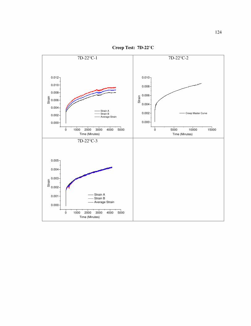
124


7D-22°C-1 7D-22°C-2

7D-22°C-3

0 1000 2000 3000 4000 5000

0.000

0.002

0.004

0.006

0.008

0.010

0.012

Strain A

Strain B

Average Strain

Str

ain

Time (Minutes)

0 5000 10000 15000

0.000

0.002

0.004

0.006

0.008

0.010

Creep Master Curve

Str

ain

Time (Minutes)

0 1000 2000 3000 4000 5000

0.000

0.001

0.002

0.003

0.004

0.005

Strain A

Strain B

Average Strain

Str

ain

Time (Minutes)

125


30D-22°C-4 30D-22°C-5

30D-22°C-6

0 1000 2000 3000 4000

0.000

0.001

0.002

0.003

0.004 Strain A

Str

ain

Time (Minutes)

0 2000 4000 6000 8000

0.000

0.001

0.002

0.003

0.004

0.005

0.006

Strain A

Strain B

Average Strain

Str

ain

Time (Minutes)

0 2000 4000 6000-0.001

0.000

0.001

0.002

0.003

0.004

0.005

0.006

Strain A

Strain B

Average Strain

Str

ain

Time (Minutes)

126


100D-22°C-7 100D-22°C-8

100D-22°C-9

0 1000 2000 3000 4000

0.0000

0.0005

0.0010

0.0015

0.0020

0.0025

0.0030

0.0035

0.0040

Strain A

Strain B

Average Strain

Str

ain

Time (Minutes) 0 1000 2000 3000 4000 5000

0.000

0.001

0.002

0.003

0.004

0.005

Strain A

Strain B

Average Strain

Str

ain

Time (Minutes)

0 500 1000 1500 2000 2500 3000-0.0005

0.0000

0.0005

0.0010

0.0015

0.0020

0.0025

0.0030

0.0035

0.0040

0.0045

Strain A

Strain B

Average Strain

Str

ain

Time (Minutes)

127

Appendix B

Validation of Time-Aging Time Superposition

Specimens from Batch 3 were tested at ages of 3, 5 and 7 days to verify the time-aging time

superposition as explained by Struik (1977) [24]. The momentary creep response for the

specimen tested at the age of 3, 5 and 7 days— i.e., the creep response for the duration of one-

tenth of the aging time (ta/10)—was utilized to create a master curve for a 7-day-old epoxy

specimen. The momentary creep response for epoxy at the age of 3 and 5 days were horizontally

shifted on the log(t) scale to superimpose the momentary creep response of 7-day-old epoxy

specimen as shown in Figure (B1).

Figure B1: Master creep curve for 7D-22°C-2 specimen.

The plot of horizontal shift factor (log a) and ageing time (log ta) also follows the

observation of Struik (1977) that creep curves shift at a constant rate with aging time as shown in

Figure (B2).

-1 0 1 2 3 4

0.0003

0.0006

0.0009

0.0012 7D-22°C-2

5D-22°C-2

3D-22°C-2

Com

plia

nce (

1/M

Pa)

log time (minutes)

128

Figure B2: Logarithm of aging time and horizontal shift showing the constant rate of increase of

shift factor.

0.0 0.2 0.4 0.6 0.8 1.0 1.2 1.4 1.63.55

3.60

3.65

3.70

3.75

3.80

3.85

3.90

3.95

4.00

4.05

Horizontal shift (log a)

log t

ime (

min

ute

s)

(ta)

R2=0.993

129

Appendix C

Matlab Code Creepmodeling

clear all; close all; clc;

syms t %user input ta & T ta=7; T=22;

%Evaluation of eqage_30 & eqbeta_30

Tg_rt=40.46+(52-40.4606)*(((ta-7)^2)/(40.7625^2+(ta-7)^2)) f=55.58*exp(2.963*10^-5*t)-15.56*exp(-0.2421*t)-Tg_rt; g=59.9*exp(8.816*10^-6*t)-19.77*exp(-0.4689*t)-Tg_rt;

eqage_30=double(solve(f)) eqage_35=double(solve(g))

eqbeta_30=double((55.58*exp(2.963*10^-5*eqage_30)-15.56*exp(-

0.2421*eqage_30)+273)/(56+273)) i=1; if ta==7 eqage_30=0 end

%evaluate creep parameter using eqbeta_30 for ct=1:10:5000

beta(ct)=double(((55.58*exp(2.963*10^-5*(eqage_30+(ct/60/24)))-

15.56*exp(-0.2421*(eqage_30+(ct/60/24)))+273))/(56+273));

if double(beta(ct))<0.955097

a(ct)=8.21*10^-5; b(ct)=0.7583; end if double(beta(ct))>0.955097 && double(beta(ct))<=0.957661 a(ct)=0.000507; b(ct)=0.4601; end if double(beta(ct))>0.957661 && double(beta(ct))<=0.960074 a(ct)=0.001606; b(ct)=0.2884; end if double(beta(ct))>0.960074 && double(beta(ct))<=0.962345 a(ct)=0.003462; b(ct)=0.1798;

130

end if double(beta(ct))>0.962345 && double(beta(ct))<=0.964483 a(ct)=0.005604; b(ct)=0.1142; end if double(beta(ct))>0.964483 && double(beta(ct))<=0.966496 a(ct)=0.007478; b(ct)=0.07596; end if double(beta(ct))>0.966496 && double(beta(ct))<=0.96839 a(ct)=0.008548; b(ct)=0.0586; end if double(beta(ct))>0.96839 && double(beta(ct))<=0.970173 a(ct)=0.009494; b(ct)=0.04522; end if double(beta(ct))>0.970173 && double(beta(ct))<=0.971852 a(ct)=0.01002; b(ct)=0.0385; end if double(beta(ct))>0.971852 && double(beta(ct))<=0.973432 a(ct)=0.01025; b(ct)=0.03568; end if double(beta(ct))>0.973432 && double(beta(ct))<=0.974919 a(ct)=0.01029; b(ct)=0.03514; end if double(beta(ct))>0.974919 && double(beta(ct))<=0.976319 a(ct)=0.01022; b(ct)=0.03594; end if double(beta(ct))>0.976319 && double(beta(ct))<=0.977637 a(ct)=0.01009; b(ct)=0.03754; end if double(beta(ct))>0.977637 && double(beta(ct))<=0.978878 a(ct)=0.009912; b(ct)=0.03963; end if double(beta(ct))>0.978878 && double(beta(ct))<=0.980046 a(ct)=0.009712; b(ct)=0.04201; end if double(beta(ct))>0.980046 && double(beta(ct))<=0.981145 a(ct)=0.0095; b(ct)=0.04458; end if double(beta(ct))>0.981145 && double(beta(ct))<=0.98218 a(ct)=0.009281; b(ct)=0.04727; end if double(beta(ct))>0.98218 && double(beta(ct))<1 a(ct)=0.00906; b(ct)=0.05003;

131

end

time(i)=ct; betatest(i)=beta(ct); %atest(i)=a(ct); %btest(i)=b(ct);

cc(i)=a(ct)*(ct+(eqage_30*24*60))^b(ct)-(a(1)*(eqage_30*24*60)^b(1)); %cc(i)=a(ct)*(ct+(eqage_30*24*60))^b(ct);

if T==30 alpha(ct)=double(((55.58*exp(2.963*10^-5*(eqage_30+(ct/60/24)))-

15.56*exp(-0.2421*(eqage_30+(ct/60/24)))+273))/(56+273)); end if T==22 alpha(ct)=((40.46+(52-40.4606)*(((ta-7+(ct/60/24))^2)/(40.7625^2+((ta-

7+(ct/60/24)))^2)))+273)/(52+273);

end if T==35 alpha(ct)=double(((59.9*exp(8.816*10^-6*(eqage_35+(ct/60/24))))-

19.77*exp(-0.4689*((eqage_35+(ct/60/24))))+273)/(60+273)); end

%Evaluation of creep activation energy

q(i)=5903*(double(alpha(ct)))^-24.9+10310;

cc(i)=cc(i)*exp(-1*q(i)/(T+273))/exp(-1*(q(i)/(30+273)));

i=i+1; end

s=transpose(cc); %p=transpose(atest); %q=transpose(btest); %r=transpose(betatest); x=1:10:5000; %plot(x,r) %plot(r,p) %plot(r,q)

plot(x,cc) hold on %plot(t_30_7,cc_30_7) %plot(t_30_30,cc_30_30)

132

%plot(t_35_30,cc_35_30) %plot(t_30_100,cc_30_100) %plot(t_RT_30,cc_RT_30) plot(t_RT_7,cc_RT_7) %plot(t_RT_100,cc_RT_100) %plot(t_35_100,cc_35_100) %plot(t_35_7,cc_35_7)

133

Appendix D

Thermoreversiblity of Physical Aging

Physical aging is a thermoreversible process. The effects of physical aging can be erased

by exposing a specimen to a temperature above its glass transition temperature. To check the

thermoreversiblity of physical aging in the epoxy resin under study, a DSC test program was

devised. A resin sample cured at 22°C for 7 days was used in this investigation. The resin sample

was subjected to temperature slightly above its Tg by heating it upto 50°C at 3°C/min from 0°C to

50°C and then quickly cooling it to 0°C in an uncontrolled manner. Another scan at the rate of

3°C/min was done on the resin sample to check if the endothermic relaxation peak, which is

present due to physical aging, was erased. As seen in Figure D1, during the first scan an

endothermic relaxation peak indicating physical aging in 7-day-old sample was observed. The Tg

of sample was 42°C. During the second scan (Figure D2) no endothermic relaxation peak was

observed but the glass transition temperature was 43°C, close to Tg value during the first scan.

Thus, it was observed (Figure D1 and Figure D2) that after exposing the resin to temperature

above its Tg, the effect of physical aging was erased but the glass transition was approximately the

same. It is expected that with the erasure of physical aging the Tg should decrease. But as the

specimen tested were only 7-day-old, the effect of physical aging was not significant enough to

influence the Tg of the resin.

134

.

Figure D1: First DSC scan showing the presence of physical aging in resin

Figure D2: Second DSC scan after exposing the specimen to temperature above its Tg

0 10 20 30 40 50 60-0.5

-0.4

-0.3

-0.2

-0.1

0.0

Heat

Flo

w (

J/g

)

Temperature (°C)

Exo

Up

Endothermic

relaxation peak

TgR1=42°C

0 10 20 30 40 50 60 70 80-0.6

-0.5

-0.4

-0.3

-0.2

-0.1

0.0

Exo U

pH

eat

Flo

w (

J/g

)

Temperature (°C)

TgR2=43°C

CHARACTERIZATION AND MODELING OF CREEP BEHAVIOR IN …

Documents

Transcript of CHARACTERIZATION AND MODELING OF CREEP BEHAVIOR IN …