CHARACTERIZATION AND COMPARISON OF PLATFORM …
84
CHARACTERIZATION AND COMPARISON OF PLATFORM REEF COMMUNITIES OFF THE TEXAS COAST by Q. R. Dokken, K. Withers, S. Childs, and T. Riggs Center for Coastal Studies Texas A&M University-Corpus Christi 6300 Ocean Drive Corpus Christi, Texas Prepared for Texas Parks and Wildlife Department Artificial Reef Program 17629 East Camino Real, Suite 175 Houston, Texas 77058 August 2000 TAMU-CC-0007-CCS
Transcript of CHARACTERIZATION AND COMPARISON OF PLATFORM …
CHARACTERIZATION AND COMPARISON OF PLATFORM REEF COMMUNITIES OFF THE TEXAS COAST
by
Q. R. Dokken, K. Withers, S. Childs, and T. Riggs
Center for Coastal Studies Texas A&M University-Corpus Christi
6300 Ocean Drive Corpus Christi, Texas
Prepared for Texas Parks and Wildlife Department
Artificial Reef Program 17629 East Camino Real, Suite 175
Houston, Texas 77058
August 2000
TAMU-CC-0007-CCS
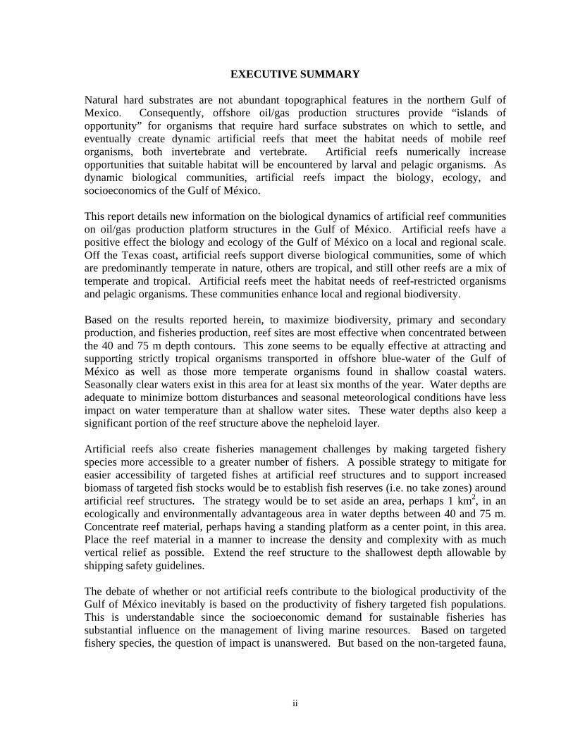
EXECUTIVE SUMMARY Natural hard substrates are not abundant topographical features in the northern Gulf of Mexico. Consequently, offshore oil/gas production structures provide “islands of opportunity” for organisms that require hard surface substrates on which to settle, and eventually create dynamic artificial reefs that meet the habitat needs of mobile reef organisms, both invertebrate and vertebrate. Artificial reefs numerically increase opportunities that suitable habitat will be encountered by larval and pelagic organisms. As dynamic biological communities, artificial reefs impact the biology, ecology, and socioeconomics of the Gulf of México. This report details new information on the biological dynamics of artificial reef communities on oil/gas production platform structures in the Gulf of México. Artificial reefs have a positive effect the biology and ecology of the Gulf of México on a local and regional scale. Off the Texas coast, artificial reefs support diverse biological communities, some of which are predominantly temperate in nature, others are tropical, and still other reefs are a mix of temperate and tropical. Artificial reefs meet the habitat needs of reef-restricted organisms and pelagic organisms. These communities enhance local and regional biodiversity. Based on the results reported herein, to maximize biodiversity, primary and secondary production, and fisheries production, reef sites are most effective when concentrated between the 40 and 75 m depth contours. This zone seems to be equally effective at attracting and supporting strictly tropical organisms transported in offshore blue-water of the Gulf of México as well as those more temperate organisms found in shallow coastal waters. Seasonally clear waters exist in this area for at least six months of the year. Water depths are adequate to minimize bottom disturbances and seasonal meteorological conditions have less impact on water temperature than at shallow water sites. These water depths also keep a significant portion of the reef structure above the nepheloid layer. Artificial reefs also create fisheries management challenges by making targeted fishery species more accessible to a greater number of fishers. A possible strategy to mitigate for easier accessibility of targeted fishes at artificial reef structures and to support increased biomass of targeted fish stocks would be to establish fish reserves (i.e. no take zones) around artificial reef structures. The strategy would be to set aside an area, perhaps 1 km2, in an ecologically and environmentally advantageous area in water depths between 40 and 75 m. Concentrate reef material, perhaps having a standing platform as a center point, in this area. Place the reef material in a manner to increase the density and complexity with as much vertical relief as possible. Extend the reef structure to the shallowest depth allowable by shipping safety guidelines. The debate of whether or not artificial reefs contribute to the biological productivity of the Gulf of México inevitably is based on the productivity of fishery targeted fish populations. This is understandable since the socioeconomic demand for sustainable fisheries has substantial influence on the management of living marine resources. Based on targeted fishery species, the question of impact is unanswered. But based on the non-targeted fauna,
ii

particularly the sessile community, the answer is unequivocally yes – artificial reefs do contribute to the biological productivity of the Gulf of México ecosystem. This report along with other reports just released and some research in progress significantly advances our understanding of the dynamics of artificial reefs. Yet, there remains a great deal of research to be done to fully understand the impact of artificial reefs upon the ecology and productivity of the Gulf of México.
iii
TABLE OF CONTENTS
PageEXECUTIVE SUMMARY ………………………………………………… iiLIST OF FIGURES…………………………………………………………. vLIST OF TABLES…………………………………………………………... viiiLIST OF APPENDICES …………………………………………………… INTRODUCTION…………………………………………………………… 1STUDY AREA……………………………………………………………….. 1
Area Description………………………………………………….…. 1Study Sites……………………………………………………………. 3
MATERIALS & METHODS…………………………………………….…. 5Water Temperature and Insolation………………………………... 5Biofouling Community……………………………………………… 7
Rugosity………………………………………………………. 7Data Analysis…………………………………………………. 7
Fish Community……………………………………………………... 8Data Analysis…………………………………………………. 8
RESULTS……………………………………………………………………. 9Abiotic Parameters……………………………………………….…. 9
Water Temperature………………………………………….... 9Insolation……………………………………………………... 10
Biofouling Community……………………………………………… 10Community Composition…………………………………….... 10Rugosity………………………………………………….…… 18Vertical Zonation……………………………………………... 18
Fish Community…………………………………………………….. 32Overall Community Composition and Structure……………… 32Comparisons of NPI 72A with Other Platforms…………….... 37
DISCUSSION………………………………………………………………... 39Biofouling Community ……………………………………………... 43Fish Community ……………………………………………………. 44Insolation and Temperature ……………………………………….. 45NPI 72A – Pre and Post-cut Communities ………………………... 46
CONCLUSION ……………………………………………………………... 47LITERATURE CITED……………………………………………………... 50APPENDICES ...…………………………………………………………….. 53
iv
LIST OF FIGURES
Figure Page
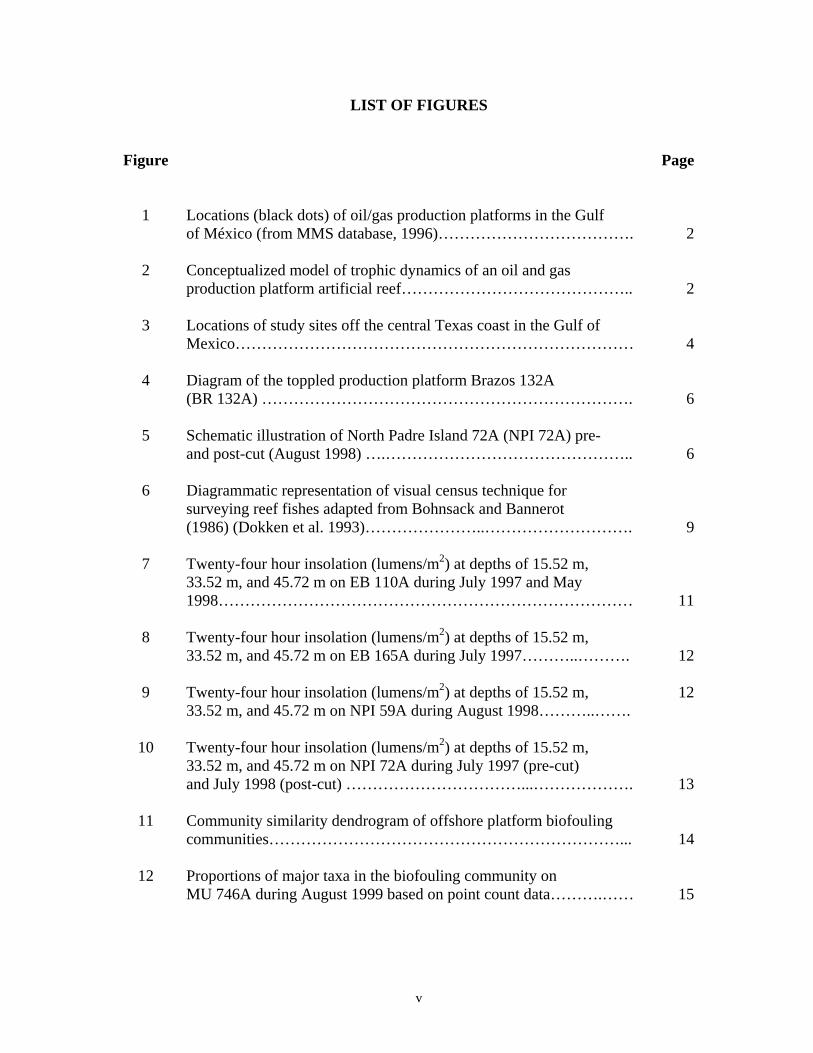
1 Locations (black dots) of oil/gas production platforms in the Gulf
of México (from MMS database, 1996)………………………………. 2 2 Conceptualized model of trophic dynamics of an oil and gas
production platform artificial reef…………………………………….. 2 3 Locations of study sites off the central Texas coast in the Gulf of
Mexico………………………………………………………………… 4 4 Diagram of the toppled production platform Brazos 132A
(BR 132A) ……………………………………………………………. 6 5 Schematic illustration of North Padre Island 72A (NPI 72A) pre-
and post-cut (August 1998) ….……………………………………….. 6 6 Diagrammatic representation of visual census technique for
surveying reef fishes adapted from Bohnsack and Bannerot (1986) (Dokken et al. 1993)…………………..………………………. 9
7 Twenty-four hour insolation (lumens/m2) at depths of 15.52 m,
33.52 m, and 45.72 m on EB 110A during July 1997 and May 1998…………………………………………………………………… 11
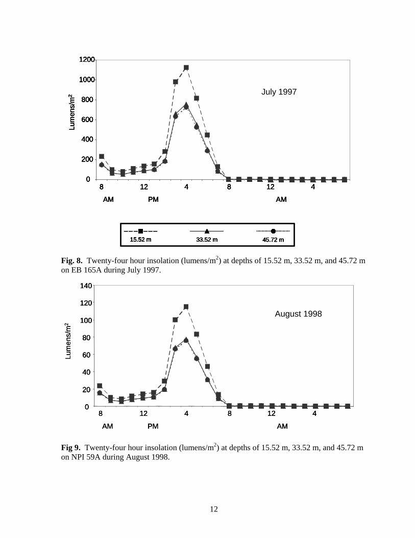
8 Twenty-four hour insolation (lumens/m2) at depths of 15.52 m,
33.52 m, and 45.72 m on EB 165A during July 1997………..………. 12 9 Twenty-four hour insolation (lumens/m2) at depths of 15.52 m,
33.52 m, and 45.72 m on NPI 59A during August 1998………..……. 12
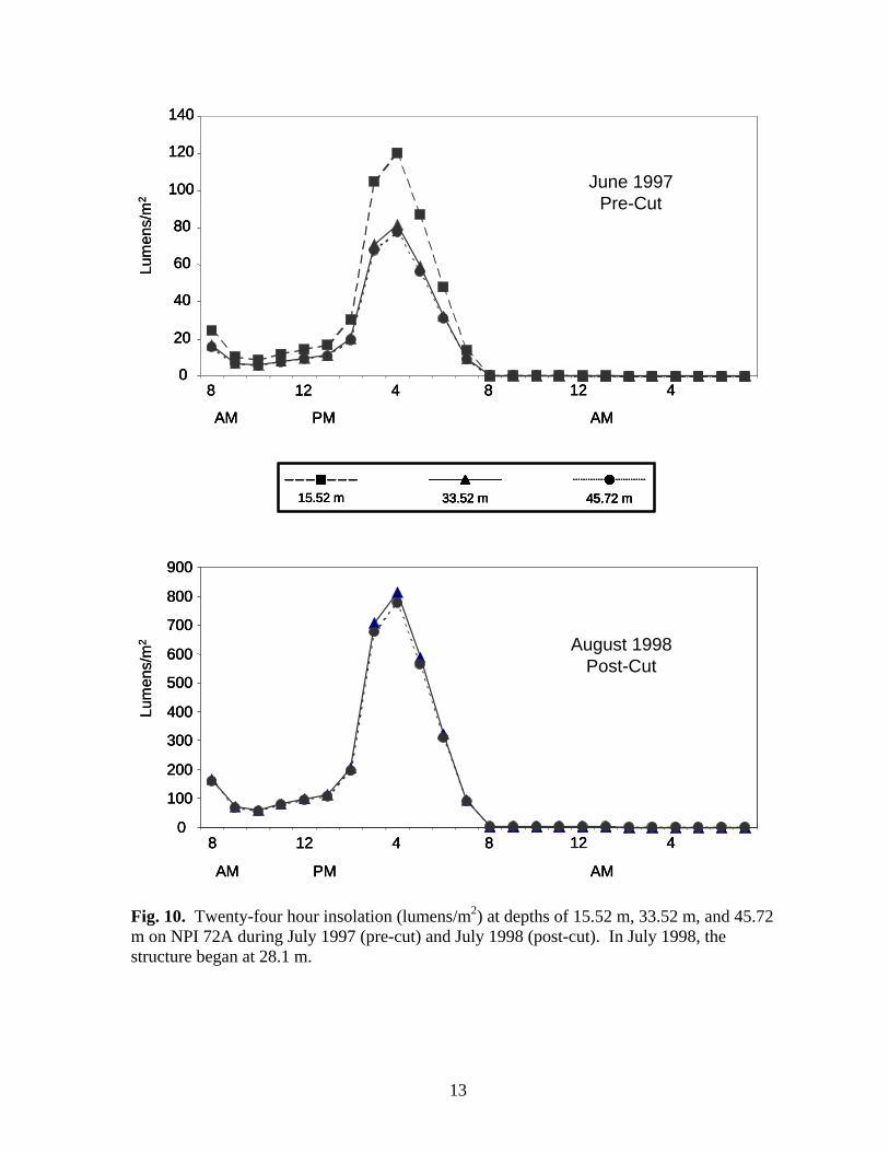
10 Twenty-four hour insolation (lumens/m2) at depths of 15.52 m,
33.52 m, and 45.72 m on NPI 72A during July 1997 (pre-cut) and July 1998 (post-cut) ……………………………...………………. 13
11 Community similarity dendrogram of offshore platform biofouling
communities…………………………………………………………... 14
12 Proportions of major taxa in the biofouling community on MU 746A during August 1999 based on point count data……….…… 15
v
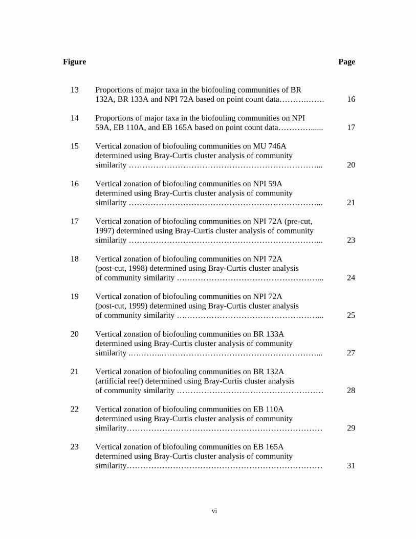
Figure Page
13 Proportions of major taxa in the biofouling communities of BR
132A, BR 133A and NPI 72A based on point count data……….……. 16
14 Proportions of major taxa in the biofouling communities on NPI 59A, EB 110A, and EB 165A based on point count data…………...... 17
15 Vertical zonation of biofouling communities on MU 746A
determined using Bray-Curtis cluster analysis of community similarity ……………………………………………………………... 20
16 Vertical zonation of biofouling communities on NPI 59A
determined using Bray-Curtis cluster analysis of community similarity ……………………………………………………………... 21
17 Vertical zonation of biofouling communities on NPI 72A (pre-cut,
1997) determined using Bray-Curtis cluster analysis of community similarity ……………………………………………………………... 23
18 Vertical zonation of biofouling communities on NPI 72A
(post-cut, 1998) determined using Bray-Curtis cluster analysis of community similarity ….…………………………………………... 24
19 Vertical zonation of biofouling communities on NPI 72A
(post-cut, 1999) determined using Bray-Curtis cluster analysis of community similarity ….…………………………………………... 25
20 Vertical zonation of biofouling communities on BR 133A
determined using Bray-Curtis cluster analysis of community similarity .….……..…………………………………………………... 27
21 Vertical zonation of biofouling communities on BR 132A
(artificial reef) determined using Bray-Curtis cluster analysis of community similarity ……………………………………………… 28
22 Vertical zonation of biofouling communities on EB 110A
determined using Bray-Curtis cluster analysis of community similarity……………………………………………………………… 29
23 Vertical zonation of biofouling communities on EB 165A
determined using Bray-Curtis cluster analysis of community similarity……………………………………………………………… 31
vi
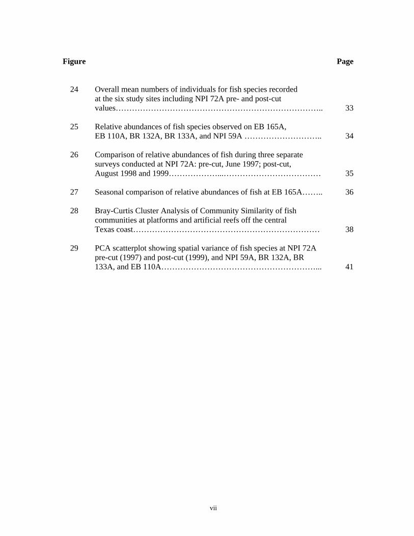
Figure Page
24 Overall mean numbers of individuals for fish species recorded
at the six study sites including NPI 72A pre- and post-cut values………………………………………………………………….. 33
25 Relative abundances of fish species observed on EB 165A,
EB 110A, BR 132A, BR 133A, and NPI 59A ……………………….. 34
26 Comparison of relative abundances of fish during three separate surveys conducted at NPI 72A: pre-cut, June 1997; post-cut, August 1998 and 1999………………...……………………………… 35
27 Seasonal comparison of relative abundances of fish at EB 165A…….. 36
28 Bray-Curtis Cluster Analysis of Community Similarity of fish communities at platforms and artificial reefs off the central Texas coast…………………………………………………………… 38
29 PCA scatterplot showing spatial variance of fish species at NPI 72A
pre-cut (1997) and post-cut (1999), and NPI 59A, BR 132A, BR 133A, and EB 110A…………………………………………………... 41
vii
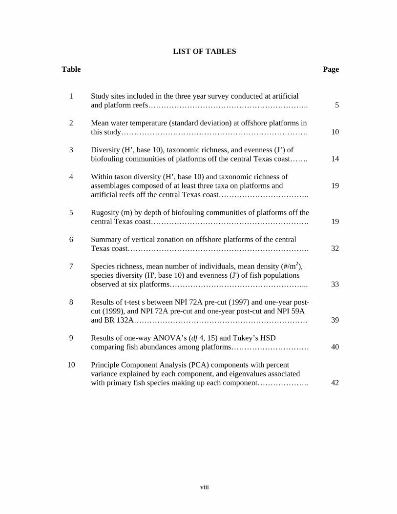
LIST OF TABLES Table Page
1 Study sites included in the three year survey conducted at artificial
and platform reefs…………………………………………………….. 5 2 Mean water temperature (standard deviation) at offshore platforms in
this study……………………………………………………………… 10 3 Diversity (H’, base 10), taxonomic richness, and evenness (J’) of
biofouling communities of platforms off the central Texas coast……. 14 4 Within taxon diversity (H’, base 10) and taxonomic richness of
assemblages composed of at least three taxa on platforms and artificial reefs off the central Texas coast……………………………..
19
5 Rugosity (m) by depth of biofouling communities of platforms off the
central Texas coast……………………………………………………. 19 6 Summary of vertical zonation on offshore platforms of the central
Texas coast……………………………………………………………. 32 7 Species richness, mean number of individuals, mean density (#/m2),
species diversity (H', base 10) and evenness (J') of fish populations observed at six platforms……………………………………………... 33
8 Results of t-test s between NPI 72A pre-cut (1997) and one-year post-
cut (1999), and NPI 72A pre-cut and one-year post-cut and NPI 59A and BR 132A…………………………………………………………. 39
9 Results of one-way ANOVA’s (df 4, 15) and Tukey’s HSD
comparing fish abundances among platforms………………………… 40
10 Principle Component Analysis (PCA) components with percent variance explained by each component, and eigenvalues associated with primary fish species making up each component……………….. 42
viii
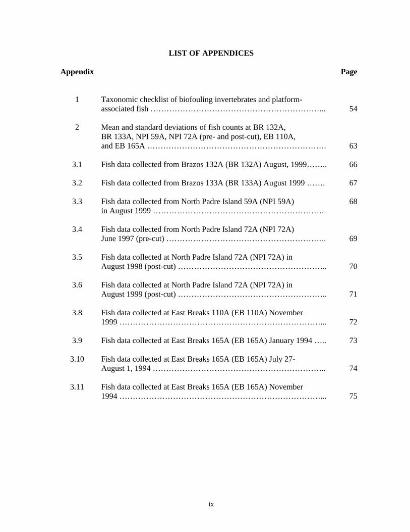
LIST OF APPENDICES
Appendix Page
1 Taxonomic checklist of biofouling invertebrates and platform-
associated fish ………………………………………………………... 54 2 Mean and standard deviations of fish counts at BR 132A,
BR 133A, NPI 59A, NPI 72A (pre- and post-cut), EB 110A, and EB 165A …………………………………………………………. 63
3.1 Fish data collected from Brazos 132A (BR 132A) August, 1999…….. 66
3.2 Fish data collected from Brazos 133A (BR 133A) August 1999 ……. 67
3.3 Fish data collected from North Padre Island 59A (NPI 59A)
in August 1999 ………………………………………………………. 68
3.4 Fish data collected from North Padre Island 72A (NPI 72A)
June 1997 (pre-cut) …………………………………………………... 69
3.5 Fish data collected at North Padre Island 72A (NPI 72A) in August 1998 (post-cut) ……………………………………………….. 70
3.6 Fish data collected at North Padre Island 72A (NPI 72A) in
August 1999 (post-cut) ……………………………………………….. 71
3.8 Fish data collected at East Breaks 110A (EB 110A) November 1999 …………………………………………………………………... 72
3.9 Fish data collected at East Breaks 165A (EB 165A) January 1994 ….. 73
3.10 Fish data collected at East Breaks 165A (EB 165A) July 27-
August 1, 1994 ……………………………………………………….. 74
3.11 Fish data collected at East Breaks 165A (EB 165A) November 1994 …………………………………………………………………... 75
ix
INTRODUCTION As artificial reefs, the approximately 5,000 oil/gas production platforms located in the northern Gulf of México (Fig. 1) support unique marine biological communities by providing solid substrates for attachment of sessile organisms and plants, cover and shelter for cryptic species, substrate for thigmotaxic species, and feeding and nursery areas for pelagic species (Fig. 2). These non-geological reef structures supplement scarce natural reef habitats in the northern Gulf of México. Because of the biological productivity (Galloway and Lewbel 1982; Dokken et al. 1993a, 1995; Dokken 1996) and socioeconomic impact (Dinton et al. 1995) of Texas’ platform reefs, many are converted to dedicated artificial reefs through a nationally recognized “Rigs to Reefs” program (Reggio 1989) after hydrocarbon production ends. Yet, ecological and biological impacts of artificial reef systems on fisheries have not been considered when formulating fishery or ecological management strategies due to lack of qualitative and quantitative data and a limited understanding of population/ecological dynamics of the habitat (Dokken et al. 1993a, 1995; Dokken 1996; Seaman 1997).
Bohnsack et al. (1997), Carr and Hixon (1997), Grossman et al. (1997) and Lindberg (1997) reviewed existing literature and questioned if existing data and knowledge support the hypothesis that artificial reefs increase regional productivity. From a fisheries perspective, it is generally accepted that artificial reefs make targeted fishery species more accessible (Ditton et al. 1995). However, in the Gulf of México, there is insufficient data to conclusively demonstrate artificial reefs enhance stocks of targeted fishery species.
Artificial reefs may benefit local/regional biodiversity, species distribution, and overall ecosystem health and productivity. However, to assess any benefit that may accrue from artificial reefs, ecosystem/habitat structure, dynamics, and linkages must be understood.
Reported herein are analyses and conclusions drawn from original data relating to biological productivity of platform reefs in the northwestern Gulf of México. Data were compiled from 1994 and 1997 to 1999. The purpose of this study was to expand understanding of ecosystem dynamics of platform artificial reefs to support development of the most effective management strategy for Texas’ artificial reef program. It was funded in part by the Texas Parks and Wildlife Department Artificial Reef Program, BP Mobil Exploration and Production, Inc., Panaco, Texas A&M University-Corpus Christi Center for Coastal Studies, and the Gulf of México Foundation.
STUDY AREA Area Description The Gulf coasts of Texas and Louisiana encompass three zoogeographic provinces, the Tamaulipan, Texan, and Austroriparian. Climate ranges from temperate to moist sub-humid in the north and arid to semiarid in the south. Onshore, southeasterly winds predominate in the areas of the Texas coast sampled for nine months of the year (spring, summer, and fall). During the remainder of the year winds fluctuate, coming from the northwest, north, northeast, east and southeast. Longshore currents generally run south to north along the
1
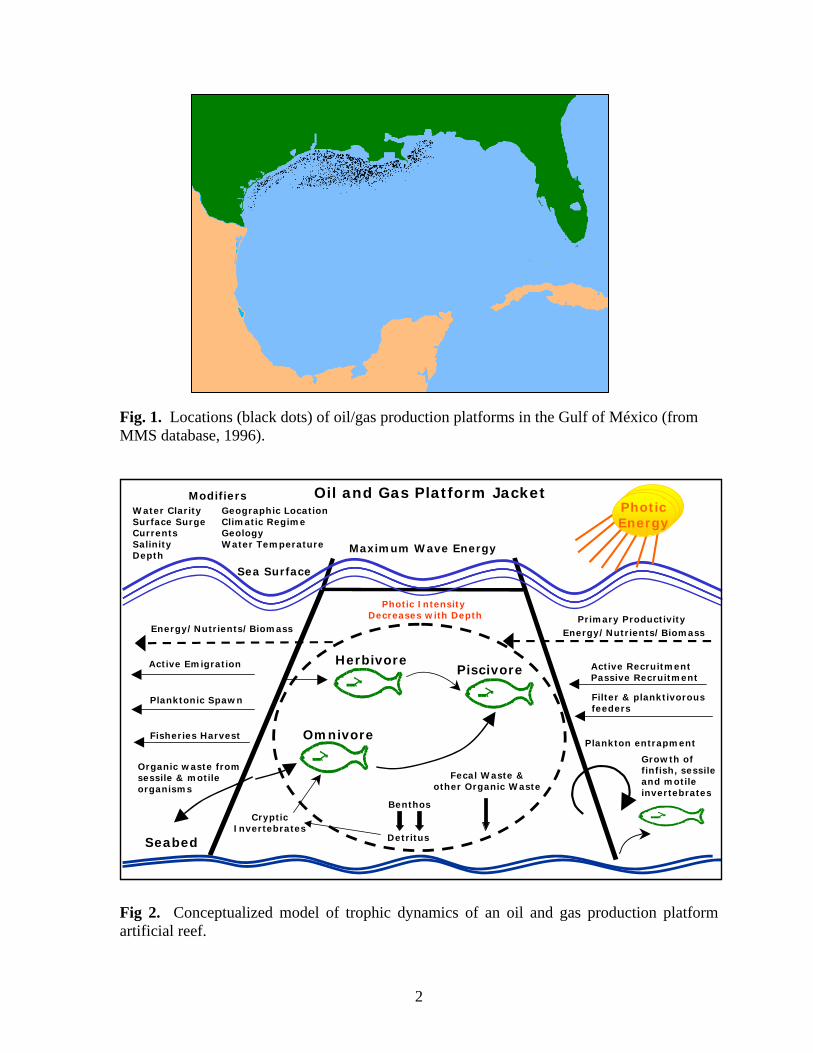
Fig. 1. Locations (black dots) of oil/gas production platforms in the Gulf of México (from MMS database, 1996).
Oil and Gas Platform JacketWater ClaritySurface SurgeCurrentsSalinityDepth
Geographic LocationClimatic RegimeGeologyWater Temperature
Modifiers
Sea Surface
Maximum Wave Energy
PhoticEnergy
Photic Intensity Decreases with Depth
Piscivore
Omnivore
Herbivore
Energy/Nutrients/Biomass
Active RecruitmentPassive Recruitment
Seabed
Benthos
Fecal Waste &other Organic Waste
Growth offinfish, sessileand motileinvertebrates
Energy/Nutrients/Biomass
Fisheries Harvest
Organic waste from sessile & motileorganisms
Filter & planktivorous feeders
Plankton entrapment
CrypticInvertebrates
Detritus
Planktonic Spawn
Active Emigration
Primary Productivity
Fig 2. Conceptualized model of trophic dynamics of an oil and gas production platform artificial reef.
2
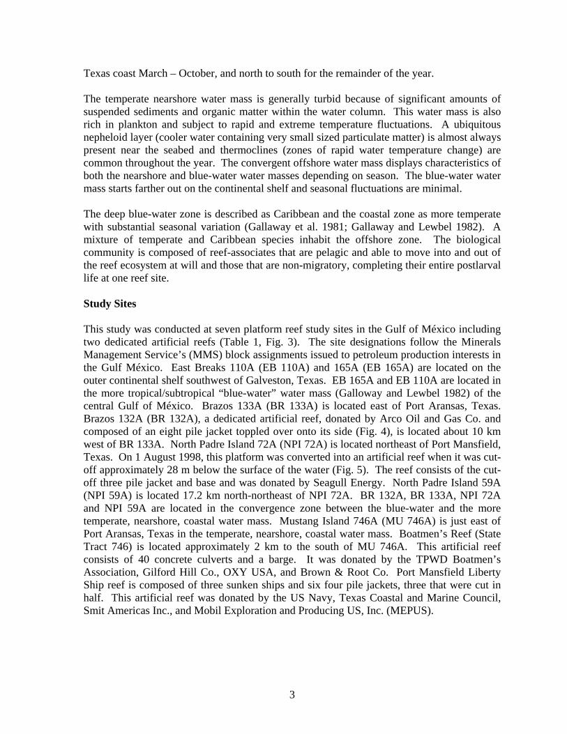
Texas coast March – October, and north to south for the remainder of the year. The temperate nearshore water mass is generally turbid because of significant amounts of suspended sediments and organic matter within the water column. This water mass is also rich in plankton and subject to rapid and extreme temperature fluctuations. A ubiquitous nepheloid layer (cooler water containing very small sized particulate matter) is almost always present near the seabed and thermoclines (zones of rapid water temperature change) are common throughout the year. The convergent offshore water mass displays characteristics of both the nearshore and blue-water water masses depending on season. The blue-water water mass starts farther out on the continental shelf and seasonal fluctuations are minimal. The deep blue-water zone is described as Caribbean and the coastal zone as more temperate with substantial seasonal variation (Gallaway et al. 1981; Gallaway and Lewbel 1982). A mixture of temperate and Caribbean species inhabit the offshore zone. The biological community is composed of reef-associates that are pelagic and able to move into and out of the reef ecosystem at will and those that are non-migratory, completing their entire postlarval life at one reef site. Study Sites This study was conducted at seven platform reef study sites in the Gulf of México including two dedicated artificial reefs (Table 1, Fig. 3). The site designations follow the Minerals Management Service’s (MMS) block assignments issued to petroleum production interests in the Gulf México. East Breaks 110A (EB 110A) and 165A (EB 165A) are located on the outer continental shelf southwest of Galveston, Texas. EB 165A and EB 110A are located in the more tropical/subtropical “blue-water” water mass (Galloway and Lewbel 1982) of the central Gulf of México. Brazos 133A (BR 133A) is located east of Port Aransas, Texas. Brazos 132A (BR 132A), a dedicated artificial reef, donated by Arco Oil and Gas Co. and composed of an eight pile jacket toppled over onto its side (Fig. 4), is located about 10 km west of BR 133A. North Padre Island 72A (NPI 72A) is located northeast of Port Mansfield, Texas. On 1 August 1998, this platform was converted into an artificial reef when it was cut-off approximately 28 m below the surface of the water (Fig. 5). The reef consists of the cut-off three pile jacket and base and was donated by Seagull Energy. North Padre Island 59A (NPI 59A) is located 17.2 km north-northeast of NPI 72A. BR 132A, BR 133A, NPI 72A and NPI 59A are located in the convergence zone between the blue-water and the more temperate, nearshore, coastal water mass. Mustang Island 746A (MU 746A) is just east of Port Aransas, Texas in the temperate, nearshore, coastal water mass. Boatmen’s Reef (State Tract 746) is located approximately 2 km to the south of MU 746A. This artificial reef consists of 40 concrete culverts and a barge. It was donated by the TPWD Boatmen’s Association, Gilford Hill Co., OXY USA, and Brown & Root Co. Port Mansfield Liberty Ship reef is composed of three sunken ships and six four pile jackets, three that were cut in half. This artificial reef was donated by the US Navy, Texas Coastal and Marine Council, Smit Americas Inc., and Mobil Exploration and Producing US, Inc. (MEPUS).
3

NPI 72A
Port MansfieldLiberty Ship
South Padre Island1070L
NPI 59A
MU 746
ST 746LBoatmen’s Reef EB 165A
EB 110A
BR 132ABR 133A
Port AransasTX
Port MansfieldTX
TEXAS
Gulf of Mexico
Brownsville TX
Galveston TX
NPI 72A
Port MansfieldLiberty Ship
South Padre Island1070L
NPI 59A
MU 746
ST 746LBoatmen’s Reef EB 165A
EB 110A
BR 132ABR 133A
Port AransasTX
Port MansfieldTX
TEXAS
Gulf of Mexico
Brownsville TX
Galveston TX
Fig. 3. Locations of study sites off the central Texas coast in the Gulf of México.
4
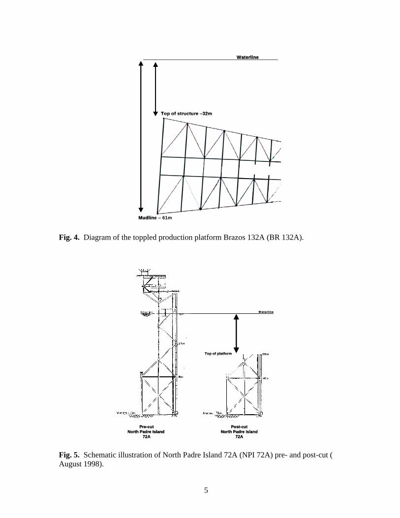
Fig. 4. Diagram of the toppled production platform Brazos 132A (BR 132A).
Waterline
Mudline – 61m
Top of structure –32m
Waterline
Mudline – 61m
Top of structure –32m
28m
Waterline
Pre-cutNorth Padre Island
72A
Post-cutNorth Padre Island
72A
Top of platform 28m28m
Waterline
Pre-cutNorth Padre Island
72A
Post-cutNorth Padre Island
72A
Top of platform
Fig. 5. Schematic illustration of North Padre Island 72A (NPI 72A) pre- and post-cut ( August 1998).
5
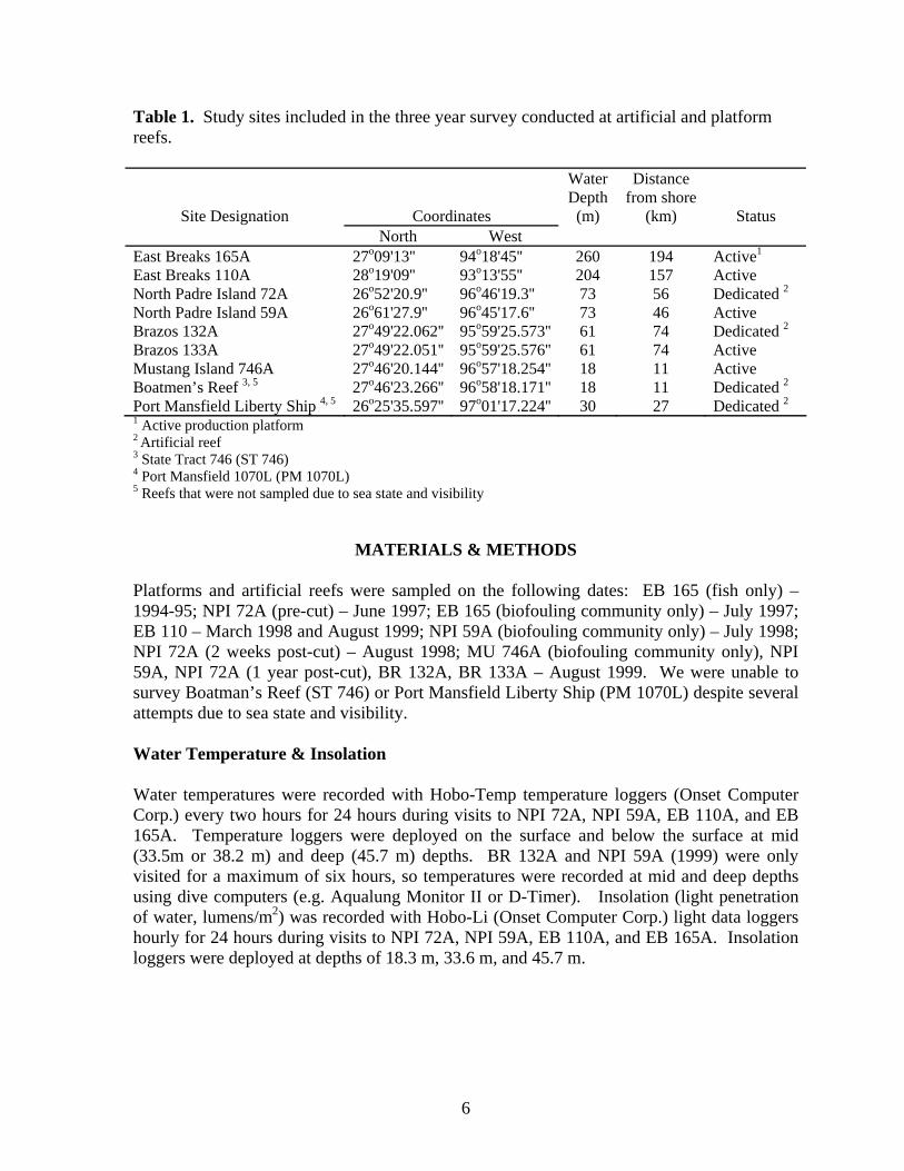
Table 1. Study sites included in the three year survey conducted at artificial and platform reefs.
Site Designation
Coordinates
Water Depth
(m)
Distance from shore
(km)
Status North West East Breaks 165A 27o09'13'' 94o18'45'' 260 194 Active1
East Breaks 110A 28o19'09'' 93o13'55'' 204 157 Active North Padre Island 72A 26o52'20.9'' 96o46'19.3'' 73 56 Dedicated 2
North Padre Island 59A 26o61'27.9'' 96o45'17.6'' 73 46 Active Brazos 132A 27o49'22.062'' 95o59'25.573'' 61 74 Dedicated 2
Brazos 133A 27o49'22.051'' 95o59'25.576'' 61 74 Active Mustang Island 746A 27o46'20.144'' 96o57'18.254'' 18 11 Active Boatmen’s Reef 3, 5 27o46'23.266'' 96o58'18.171'' 18 11 Dedicated 2
Port Mansfield Liberty Ship 4, 5 26o25'35.597'' 97o01'17.224'' 30 27 Dedicated 2
1 Active production platform 2 Artificial reef 3 State Tract 746 (ST 746) 4 Port Mansfield 1070L (PM 1070L) 5 Reefs that were not sampled due to sea state and visibility
MATERIALS & METHODS Platforms and artificial reefs were sampled on the following dates: EB 165 (fish only) – 1994-95; NPI 72A (pre-cut) – June 1997; EB 165 (biofouling community only) – July 1997; EB 110 – March 1998 and August 1999; NPI 59A (biofouling community only) – July 1998; NPI 72A (2 weeks post-cut) – August 1998; MU 746A (biofouling community only), NPI 59A, NPI 72A (1 year post-cut), BR 132A, BR 133A – August 1999. We were unable to survey Boatman’s Reef (ST 746) or Port Mansfield Liberty Ship (PM 1070L) despite several attempts due to sea state and visibility. Water Temperature & Insolation Water temperatures were recorded with Hobo-Temp temperature loggers (Onset Computer Corp.) every two hours for 24 hours during visits to NPI 72A, NPI 59A, EB 110A, and EB 165A. Temperature loggers were deployed on the surface and below the surface at mid (33.5m or 38.2 m) and deep (45.7 m) depths. BR 132A and NPI 59A (1999) were only visited for a maximum of six hours, so temperatures were recorded at mid and deep depths using dive computers (e.g. Aqualung Monitor II or D-Timer). Insolation (light penetration of water, lumens/m2) was recorded with Hobo-Li (Onset Computer Corp.) light data loggers hourly for 24 hours during visits to NPI 72A, NPI 59A, EB 110A, and EB 165A. Insolation loggers were deployed at depths of 18.3 m, 33.6 m, and 45.7 m.
6
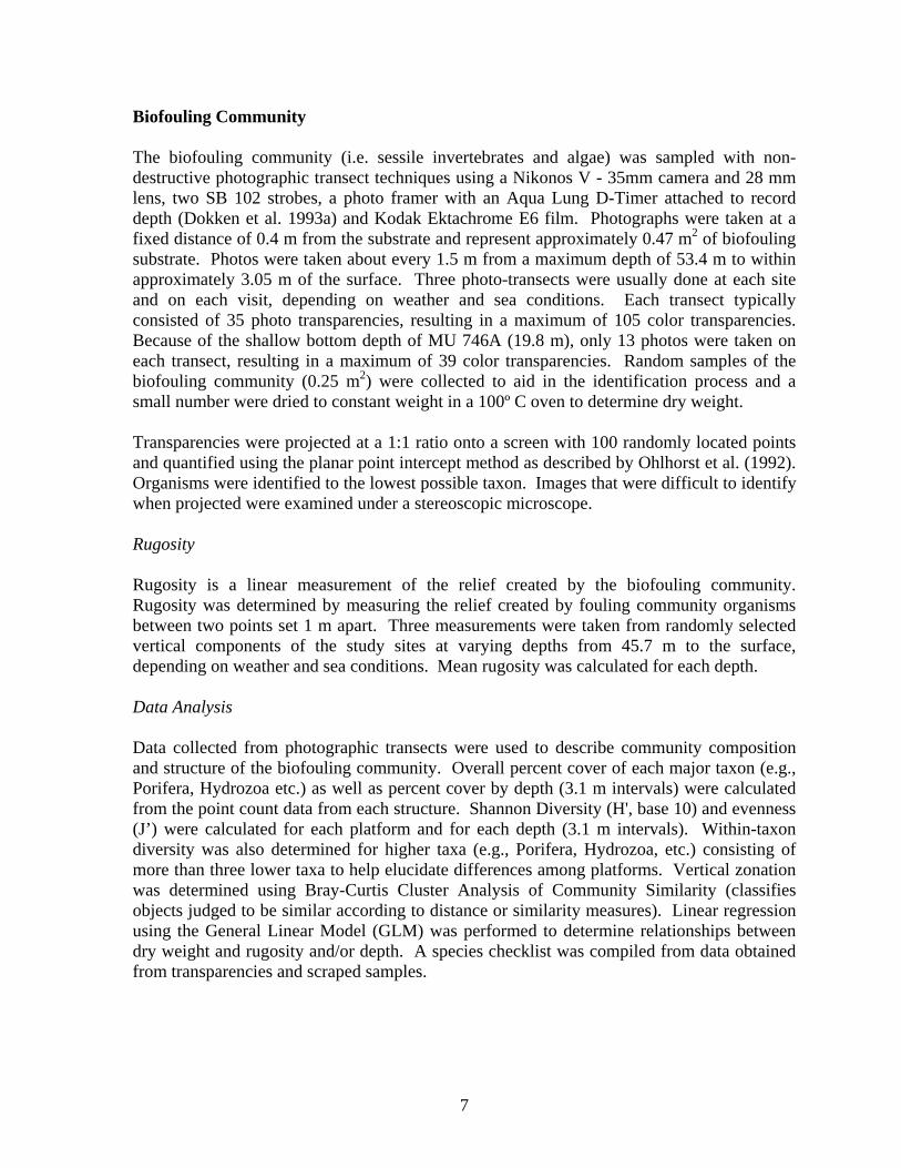
Biofouling Community The biofouling community (i.e. sessile invertebrates and algae) was sampled with non-destructive photographic transect techniques using a Nikonos V - 35mm camera and 28 mm lens, two SB 102 strobes, a photo framer with an Aqua Lung D-Timer attached to record depth (Dokken et al. 1993a) and Kodak Ektachrome E6 film. Photographs were taken at a fixed distance of 0.4 m from the substrate and represent approximately 0.47 m2 of biofouling substrate. Photos were taken about every 1.5 m from a maximum depth of 53.4 m to within approximately 3.05 m of the surface. Three photo-transects were usually done at each site and on each visit, depending on weather and sea conditions. Each transect typically consisted of 35 photo transparencies, resulting in a maximum of 105 color transparencies. Because of the shallow bottom depth of MU 746A (19.8 m), only 13 photos were taken on each transect, resulting in a maximum of 39 color transparencies. Random samples of the biofouling community (0.25 m2) were collected to aid in the identification process and a small number were dried to constant weight in a 100º C oven to determine dry weight. Transparencies were projected at a 1:1 ratio onto a screen with 100 randomly located points and quantified using the planar point intercept method as described by Ohlhorst et al. (1992). Organisms were identified to the lowest possible taxon. Images that were difficult to identify when projected were examined under a stereoscopic microscope. Rugosity Rugosity is a linear measurement of the relief created by the biofouling community. Rugosity was determined by measuring the relief created by fouling community organisms between two points set 1 m apart. Three measurements were taken from randomly selected vertical components of the study sites at varying depths from 45.7 m to the surface, depending on weather and sea conditions. Mean rugosity was calculated for each depth.
Data Analysis Data collected from photographic transects were used to describe community composition and structure of the biofouling community. Overall percent cover of each major taxon (e.g., Porifera, Hydrozoa etc.) as well as percent cover by depth (3.1 m intervals) were calculated from the point count data from each structure. Shannon Diversity (H', base 10) and evenness (J’) were calculated for each platform and for each depth (3.1 m intervals). Within-taxon diversity was also determined for higher taxa (e.g., Porifera, Hydrozoa, etc.) consisting of more than three lower taxa to help elucidate differences among platforms. Vertical zonation was determined using Bray-Curtis Cluster Analysis of Community Similarity (classifies objects judged to be similar according to distance or similarity measures). Linear regression using the General Linear Model (GLM) was performed to determine relationships between dry weight and rugosity and/or depth. A species checklist was compiled from data obtained from transparencies and scraped samples.
7
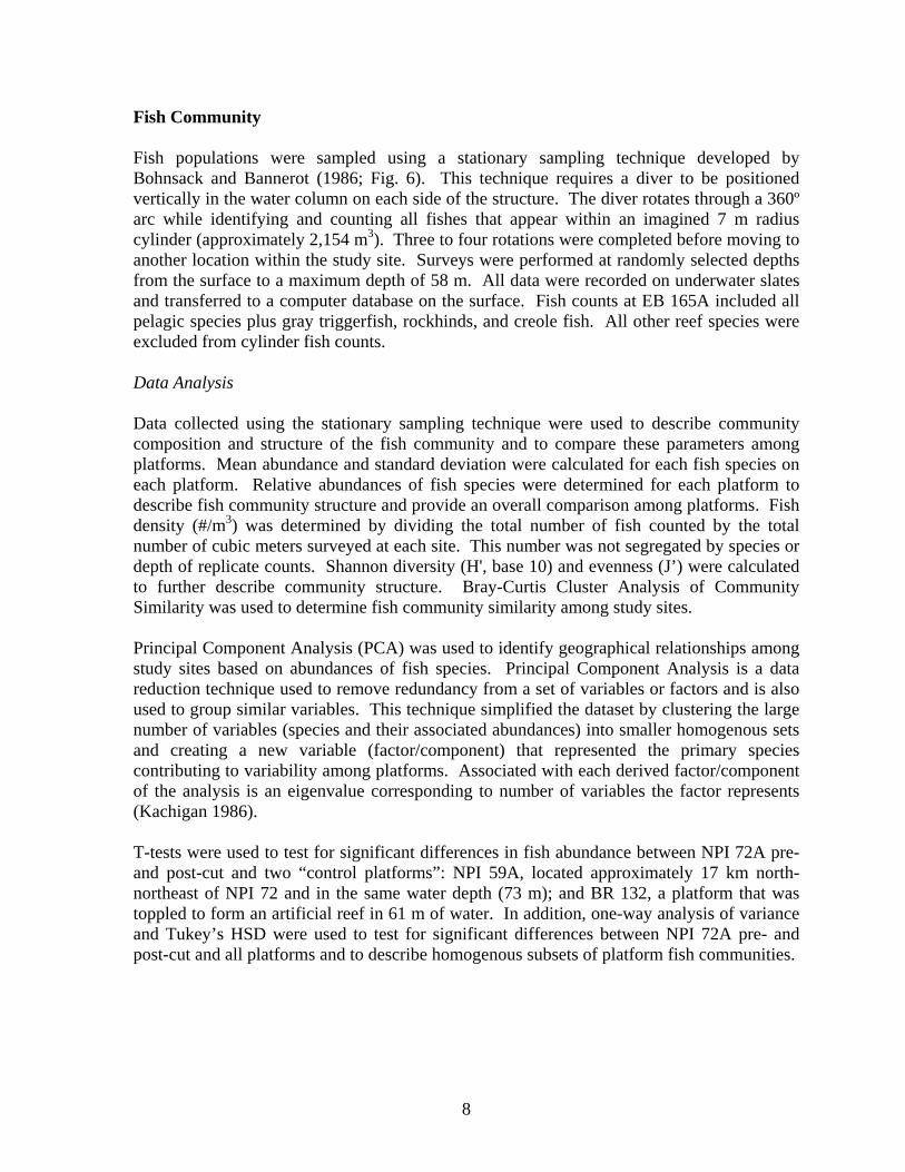
Fish Community Fish populations were sampled using a stationary sampling technique developed by Bohnsack and Bannerot (1986; Fig. 6). This technique requires a diver to be positioned vertically in the water column on each side of the structure. The diver rotates through a 360º arc while identifying and counting all fishes that appear within an imagined 7 m radius cylinder (approximately 2,154 m3). Three to four rotations were completed before moving to another location within the study site. Surveys were performed at randomly selected depths from the surface to a maximum depth of 58 m. All data were recorded on underwater slates and transferred to a computer database on the surface. Fish counts at EB 165A included all pelagic species plus gray triggerfish, rockhinds, and creole fish. All other reef species were excluded from cylinder fish counts. Data Analysis Data collected using the stationary sampling technique were used to describe community composition and structure of the fish community and to compare these parameters among platforms. Mean abundance and standard deviation were calculated for each fish species on each platform. Relative abundances of fish species were determined for each platform to describe fish community structure and provide an overall comparison among platforms. Fish density (#/m3) was determined by dividing the total number of fish counted by the total number of cubic meters surveyed at each site. This number was not segregated by species or depth of replicate counts. Shannon diversity (H', base 10) and evenness (J’) were calculated to further describe community structure. Bray-Curtis Cluster Analysis of Community Similarity was used to determine fish community similarity among study sites. Principal Component Analysis (PCA) was used to identify geographical relationships among study sites based on abundances of fish species. Principal Component Analysis is a data reduction technique used to remove redundancy from a set of variables or factors and is also used to group similar variables. This technique simplified the dataset by clustering the large number of variables (species and their associated abundances) into smaller homogenous sets and creating a new variable (factor/component) that represented the primary species contributing to variability among platforms. Associated with each derived factor/component of the analysis is an eigenvalue corresponding to number of variables the factor represents (Kachigan 1986). T-tests were used to test for significant differences in fish abundance between NPI 72A pre- and post-cut and two “control platforms”: NPI 59A, located approximately 17 km north-northeast of NPI 72 and in the same water depth (73 m); and BR 132, a platform that was toppled to form an artificial reef in 61 m of water. In addition, one-way analysis of variance and Tukey’s HSD were used to test for significant differences between NPI 72A pre- and post-cut and all platforms and to describe homogenous subsets of platform fish communities.
8
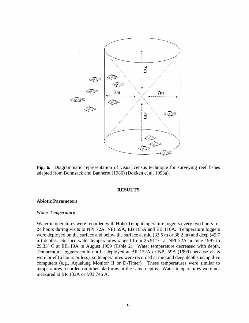
Fig. 6. Diagrammatic representation of visual census technique for surveying reef fishes adapted from Bohnsack and Bannerot (1986) (Dokken et al. 1993a).
RESULTS
Abiotic Parameters Water Temperature Water temperatures were recorded with Hobo Temp temperature loggers every two hours for 24 hours during visits to NPI 72A, NPI 59A, EB 165A and EB 110A. Temperature loggers were deployed on the surface and below the surface at mid (33.5 m or 38.2 m) and deep (45.7 m) depths. Surface water temperatures ranged from 25.91º C at NPI 72A in June 1997 to 29.33º C at EB110A in August 1999 (Table 2). Water temperature decreased with depth. Temperature loggers could not be deployed at BR 132A or NPI 59A (1999) because visits were brief (6 hours or less), so temperatures were recorded at mid and deep depths using dive computers (e.g., Aqualung Monitor II or D-Timer). These temperatures were similar to temperatures recorded on other platforms at the same depths. Water temperatures were not measured at BR 133A or MU 746 A.
9
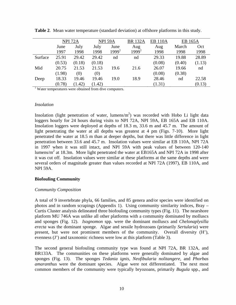
Table 2. Mean water temperature (standard deviation) at offshore platforms in this study.
NPI 72A NPI 59A BR 132A EB 110A EB 165A
June 1997
July 1998
July 1998
June 19991
Aug 19991
Aug 1998
March 1998
Oct 1998
Surface 25.91 (0.53)
29.42 (0.18)
29.42 (0.18)
nd nd 29.33 (0.08)
19.88 (0.40)
28.89 (1.13)
Mid 20.75 (1.98)
21.53 (0)
21.53 (0)
19.6 21.6 26.07 (0.08)
19.66 (0.38)
nd
Deep 18.33 (0.78)
19.46 (1.42)
19.46 (1.42)
19.0 18.9 28.46 (1.31)
nd 22.58 (0.13)
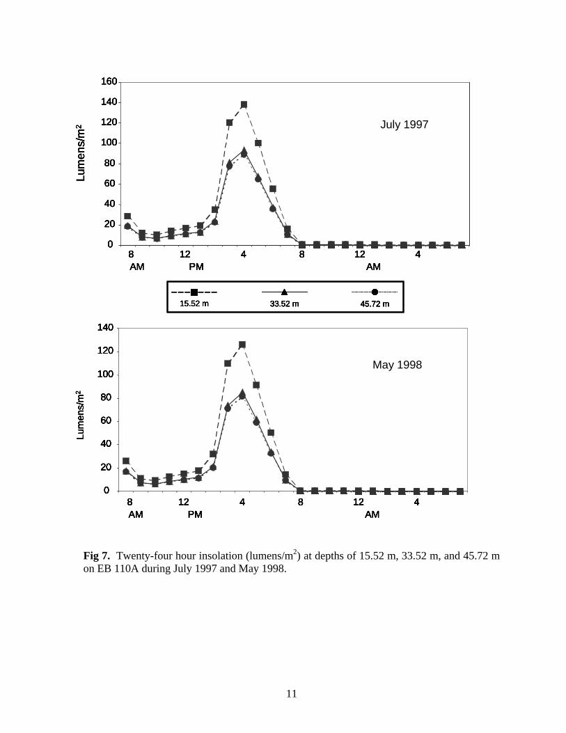
1 Water temperatures were obtained from dive computers. Insolation Insolation (light penetration of water, lumens/m2) was recorded with Hobo Li light data loggers hourly for 24 hours during visits to NPI 72A, NPI 59A, EB 165A and EB 110A. Insolation loggers were deployed at depths of 18.3 m, 33.6 m and 45.7 m. The amount of light penetrating the water at all depths was greatest at 4 pm (Figs. 7-10). More light penetrated the water at 18.5 m than at deeper depths, but there was little difference in light penetration between 33.6 and 45.7 m. Insolation values were similar at EB 110A, NPI 72A in 1997 when it was still intact, and NPI 59A with peak values of between 120-140 lumens/m2 at 18.3m. More light penetrated the water at EB165A and NPI 72A in 1998 after it was cut off. Insolation values were similar at these platforms at the same depths and were several orders of magnitude greater than values recorded at NPI 72A (1997), EB 110A, and NPI 59A. Biofouling Community Community Composition A total of 9 invertebrate phyla, 66 families, and 85 genera and/or species were identified on photos and in random scrapings (Appendix 1). Using community similarity indices, Bray – Curtis Cluster analysis delineated three biofouling community types (Fig. 11). The nearshore platform MU 746A was unlike all other platforms with a community dominated by molluscs and sponges (Fig. 12). Isognomon spp. were the dominant molluscs and Chelonaplysilla erecta was the dominant sponge. Algae and sessile hydrozoans (primarily Sertularia) were present, but were not prominent members of the community. Overall diversity (H’), evenness (J’) and taxonomic richness were low at this platform (Table 3). The second general biofouling community type was found at NPI 72A, BR 132A, and BR133A. The communities on these platforms were generally dominated by algae and sponges (Fig. 13). The sponges Tedania ignis, Neofibularia nolitangere, and Phorbas amaranthus were the dominant species. Algae were not differentiated. The next most common members of the community were typically bryozoans, primarily Bugula spp., and
10
0
20
40
60
80
100
120
140
Lum
ens/
m2
0
20
40
60
80
100
120
140
160Lu
men
s/m
2
8 12 4 8 12 4AM PM AM
8 12 4 8 12 4AM PM AM
July 1997
May 1998
15.52 m 33.52 m 45.72 m
0
20
40
60
80
100
120
140
Lum
ens/
m2
0
20
40
60
80
100
120
140
160Lu
men
s/m
2
8 12 4 8 12 4AM PM AM
8 12 4 8 12 4AM PM AM
July 1997
May 1998
0
20
40
60
80
100
120
140
Lum
ens/
m2
0
20
40
60
80
100
120
140
160Lu
men
s/m
2
8 12 4 8 12 4AM PM AM
8 12 4 8 12 4AM PM AM
0
20
40
60
80
100
120
140
0
20
40
60
80
100
120
140
Lum
ens/
m2
0
20
40
60
80
100
120
140
160
0
20
40
60
80
100
120
140
160Lu
men
s/m
2
8 12 4 8 12 4AM PM AM8 12 4 8 12 4AM PM AM
8 12 4 8 12 4AM PM AM8 12 4 8 12 4AM PM AM
July 1997
May 1998
15.52 m 33.52 m 45.72 m15.52 m15.52 m 33.52 m33.52 m 45.72 m45.72 m
Fig 7. Twenty-four hour insolation (lumens/m2) at depths of 15.52 m, 33.52 m, and 45.72 m on EB 110A during July 1997 and May 1998.
11
15.52 m 33.52 m 45.72 m
8 12 4 8 12 4
AM PM AM
0
200
400
600
800
1000
1200
Lum
ens/
m2 July 1997
15.52 m 33.52 m 45.72 m
8 12 4 8 12 4
AM PM AM
0
200
400
600
800
1000
1200
Lum
ens/
m2
15.52 m 33.52 m 45.72 m15.52 m15.52 m 33.52 m33.52 m 45.72 m45.72 m
8 12 4 8 12 4
AM PM AM
0
200
400
600
800
1000
1200
Lum
ens/
m2
8 12 4 8 12 4
AM PM AM
8 12 4 8 12 4
AM PM AM
0
200
400
600
800
1000
1200
0
200
400
600
800
1000
1200
Lum
ens/
m2 July 1997
Fig. 8. Twenty-four hour insolation (lumens/m2) at depths of 15.52 m, 33.52 m, and 45.72 m on EB 165A during July 1997.
Fig 9. Twenty-four hour insolation (lumens/m2) at depths of 15.52 m, 33.52 m, and 45.72 m on NPI 59A during August 1998.
0
20
40
60
80
100
120
140
August 1998
8 12 4 8 12 4
AM PM AM
Lum
ens/
m2
0
20
40
60
80
100
120
140
0
20
40
60
80
100
120
140
August 1998
8 12 4 8 12 4
AM PM AM
8 12 4 8 12 4
AM PM AM
Lum
ens/
m2
12
0
20
40
60
80
100
120
140
0
100
200
300
400
500
600
700
800
900
15.52 m 33.52 m 45.72 m
Lum
ens/
m2
Lum
ens/
m2
8 12 4 8 12 4
AM PM AM
8 12 4 8 12 4
AM PM AM
June 1997Pre-Cut
August 1998Post-Cut
0
20
40
60
80
100
120
140
0
20
40
60
80
100
120
140
0
100
200
300
400
500
600
700
800
900
0
100
200
300
400
500
600
700
800
900
15.52 m 33.52 m 45.72 m15.52 m15.52 m 33.52 m33.52 m 45.72 m45.72 m
Lum
ens/
m2
Lum
ens/
m2
8 12 4 8 12 4
AM PM AM
8 12 4 8 12 4
AM PM AM
8 12 4 8 12 4
AM PM AM
8 12 4 8 12 4
AM PM AM
June 1997Pre-Cut
August 1998Post-Cut
Fig. 10. Twenty-four hour insolation (lumens/m2) at depths of 15.52 m, 33.52 m, and 45.72 m on NPI 72A during July 1997 (pre-cut) and July 1998 (post-cut). In July 1998, the structure began at 28.1 m.
13
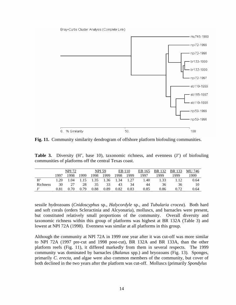
Fig. 11. Community similarity dendrogram of offshore platform biofouling communities. Table 3. Diversity (H’, base 10), taxonomic richness, and evenness (J’) of biofouling communities of platforms off the central Texas coast.
NPI 72 NPI 59 EB 110 EB 165 BR 132 BR 133 MU 746
1997 1998 1999 1998 1999 1998 1999 1997 1999 1999 1999 H’ 1.20 1.04 1.15 1.35 1.36 1.34 1.27 1.40 1.33 1.12 0.64 Richness 30 27 28 35 33 43 34 44 36 36 10 J’ 0.81 0.70 0.79 0.88 0.89 0.82 0.83 0.85 0.86 0.72 0.64
sessile hydrozoans (Cnidoscyphus sp., Halycordyle sp., and Tubularia crocea). Both hard and soft corals (orders Scleractinia and Alcyonaria), molluscs, and barnacles were present, but constituted relatively small proportions of the community. Overall diversity and taxonomic richness within this group of platforms was highest at BR 132A (Table 3) and lowest at NPI 72A (1998). Evenness was similar at all platforms in this group. Although the community at NPI 72A in 1999 one year after it was cut-off was more similar to NPI 72A (1997 pre-cut and 1998 post-cut), BR 132A and BR 133A, than the other platform reefs (Fig. 11), it differed markedly from them in several respects. The 1999 community was dominated by barnacles (Balanus spp.) and bryozoans (Fig. 13). Sponges, primarily C. erecta, and algae were also common members of the community, but cover of both declined in the two years after the platform was cut-off. Molluscs (primarily Spondylus
14
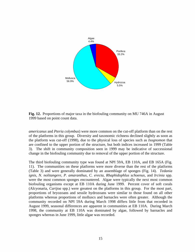
Porifera33.2%
Hydrozoa5.5%
Mollusca56.9%
Algae4.4%
Fig. 12. Proportions of major taxa in the biofouling community on MU 746A in August 1999 based on point count data. americanus and Pteria colymbus) were more common on the cut-off platform than on the rest of the platforms in this group. Diversity and taxonomic richness declined slightly as soon as the platform was cut-off (1998), due to the physical loss of species such as Isognomon that are confined to the upper portion of the structure, but both indices increased in 1999 (Table 3). The shift in community composition seen in 1999 may be indicative of successional change in the biofouling community due to removal of the upper portion of the structure. The third biofouling community type was found at NPI 59A, EB 110A, and EB 165A (Fig. 11). The communities on these platforms were more diverse than the rest of the platforms (Table 3) and were generally dominated by an assemblage of sponges (Fig. 14). Tedania ignis, N. nolitangere, P. amaranthus, C. erecta, Rhaphidophlus schoenus, and Ircinia spp. were the most common sponges encountered. Algae were typically the next most common biofouling organisms except at EB 110A during June 1999. Percent cover of soft corals (Alcyonaria, Carijoa spp.) were greatest on the platforms in this group. For the most part, proportions of bryozoans and sessile hydrozoans were similar to those found on all other platforms whereas proportions of molluscs and barnacles were often greater. Although the community recorded on NPI 59A during March 1998 differs little from that recorded in August 1999, seasonal differences are apparent in communities at EB 110A. During March 1998, the community at EB 110A was dominated by algae, followed by barnacles and sponges whereas in June 1999, little algae was recorded.
15
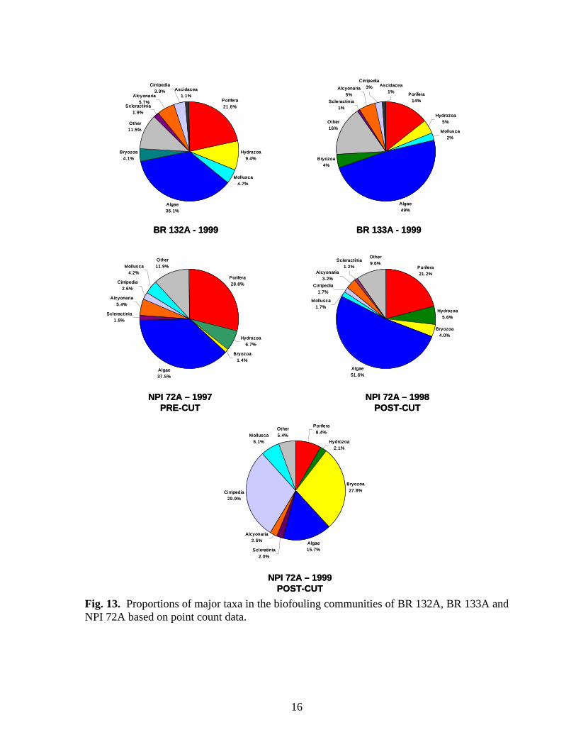
Porifera21.6%
Hydrozoa9.4%
Mollusca4.7%
Algae36.1%
Bryozoa4.1%
Other11.5%
Ascidacea1.1%
Scleractinia1.9%
Alcyonaria5.7%
Cirripedia3.9%
BR 132A - 1999
Porifera14%
Hydrozoa5%
Mollusca2%
Algae49%
Bryozoa4%
Other16%
Scleractinia1%
Alcyonaria5%
Ascidacea1%
Cirripedia3%
BR 133A - 1999
Porifera28.8%
Hydrozoa6.7%
Bryozoa1.4%
Algae37.5%
Scleractinia1.5%
Alcyonaria5.4%
Cirripedia2.6%
Mollusca4.2%
Other11.9%
NPI 72A – 1997PRE-CUT
NPI 72A – 1998POST-CUT
Porifera8.4%
Hydrozoa2.1%
Bryozoa27.8%
Algae15.7%Scleratinia
2.0%
Alcyonaria2.5%
Cirripedia29.9%
Mollusca6.1%
Other5.4%
NPI 72A – 1999POST-CUT
Porifera21.2%
Hydrozoa5.6%
Bryozoa4.0%
Algae51.6%
Alcyonaria3.2%
Scleractinia1.2%
Other9.6%
Cirripedia1.7%
Mollusca1.7%
Fig. 13. Proportions of major taxa in the biofouling communities of BR 132A, BR 133A and NPI 72A based on point count data.
16
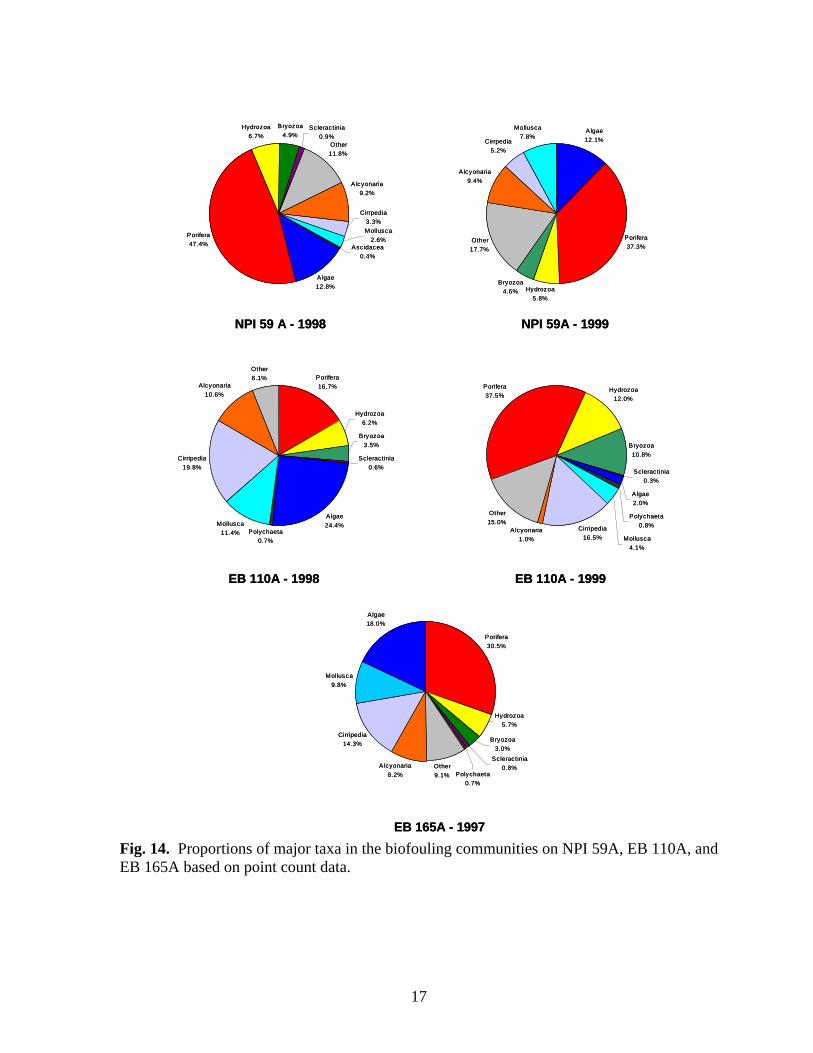
Porifera47.4%
Hydrozoa6.7%
Other11.8%
Bryozoa4.9%
Scleractinia0.9%
Alcyonaria9.2%
Algae12.8%
Ascidacea0.4%
Mollusca2.6%
Cirrpedia3.3%
NPI 59 A - 1998
Algae12.1%
Porifera37.3%
Hydrozoa5.8%
Bryozoa4.6%
Other17.7%
Alcyonaria9.4%
Cirrpedia5.2%
Mollusca7.8%
NPI 59A - 1999
Porifera16.7%
Hydrozoa6.2%
Bryozoa3.5%
Algae24.4%
Polychaeta0.7%
Mollusca11.4%
Cirripedia19.8%
Alcyonaria10.6%
Other6.1%
Scleractinia0.6%
EB 110A - 1998
Porifera37.5%
Hydrozoa12.0%
Bryozoa10.8%
Scleractinia0.3%
Algae2.0%
Polychaeta0.8%
Mollusca4.1%
Cirripedia16.5%
Alcyonaria1.0%
Other15.0%
EB 110A - 1999
EB 165A - 1997
Porifera30.5%
Alcyonaria8.2%
Cirripedia14.3%
Mollusca9.8%
Algae18.0%
Hydrozoa5.7%
Bryozoa3.0%
Other9.1%
Scleractinia0.8%
Polychaeta0.7%
Fig. 14. Proportions of major taxa in the biofouling communities on NPI 59A, EB 110A, and EB 165A based on point count data.
17
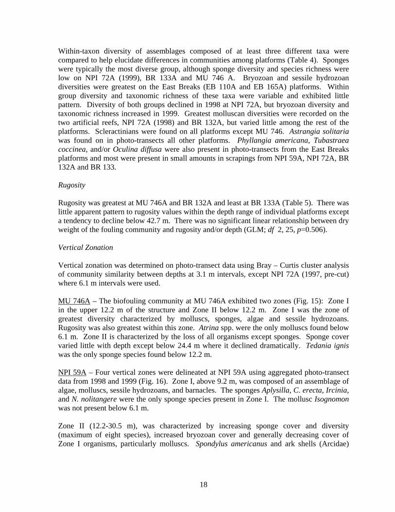
Within-taxon diversity of assemblages composed of at least three different taxa were compared to help elucidate differences in communities among platforms (Table 4). Sponges were typically the most diverse group, although sponge diversity and species richness were low on NPI 72A (1999), BR 133A and MU 746 A. Bryozoan and sessile hydrozoan diversities were greatest on the East Breaks (EB 110A and EB 165A) platforms. Within group diversity and taxonomic richness of these taxa were variable and exhibited little pattern. Diversity of both groups declined in 1998 at NPI 72A, but bryozoan diversity and taxonomic richness increased in 1999. Greatest molluscan diversities were recorded on the two artificial reefs, NPI 72A (1998) and BR 132A, but varied little among the rest of the platforms. Scleractinians were found on all platforms except MU 746. Astrangia solitaria was found on in photo-transects all other platforms. Phyllangia americana, Tubastraea coccinea, and/or Oculina diffusa were also present in photo-transects from the East Breaks platforms and most were present in small amounts in scrapings from NPI 59A, NPI 72A, BR 132A and BR 133. Rugosity
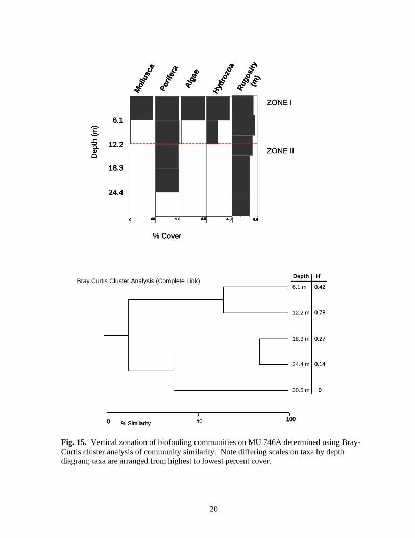
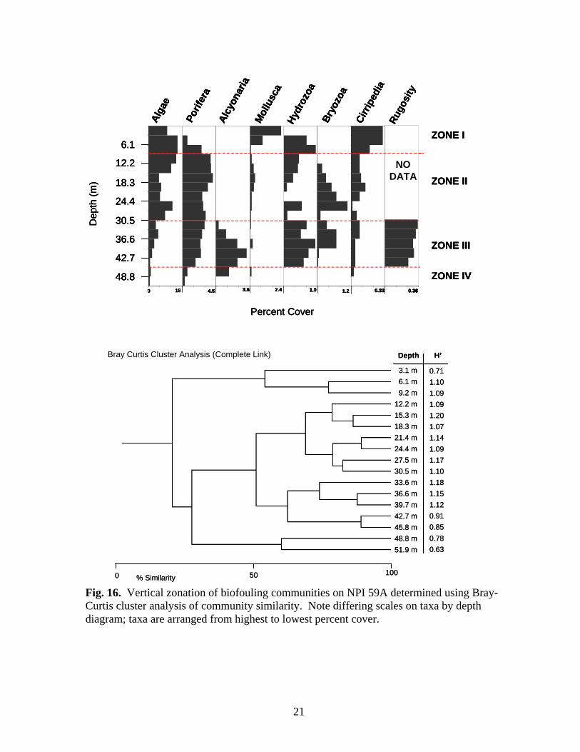
Rugosity was greatest at MU 746A and BR 132A and least at BR 133A (Table 5). There was little apparent pattern to rugosity values within the depth range of individual platforms except a tendency to decline below 42.7 m. There was no significant linear relationship between dry weight of the fouling community and rugosity and/or depth (GLM; df 2, 25, p=0.506). Vertical Zonation Vertical zonation was determined on photo-transect data using Bray – Curtis cluster analysis of community similarity between depths at 3.1 m intervals, except NPI 72A (1997, pre-cut) where 6.1 m intervals were used. MU 746A – The biofouling community at MU 746A exhibited two zones (Fig. 15): Zone I in the upper 12.2 m of the structure and Zone II below 12.2 m. Zone I was the zone of greatest diversity characterized by molluscs, sponges, algae and sessile hydrozoans. Rugosity was also greatest within this zone. Atrina spp. were the only molluscs found below 6.1 m. Zone II is characterized by the loss of all organisms except sponges. Sponge cover varied little with depth except below 24.4 m where it declined dramatically. Tedania ignis was the only sponge species found below 12.2 m. NPI 59A – Four vertical zones were delineated at NPI 59A using aggregated photo-transect data from 1998 and 1999 (Fig. 16). Zone I, above 9.2 m, was composed of an assemblage of algae, molluscs, sessile hydrozoans, and barnacles. The sponges Aplysilla, C. erecta, Ircinia, and N. nolitangere were the only sponge species present in Zone I. The mollusc Isognomon was not present below 6.1 m. Zone II (12.2-30.5 m), was characterized by increasing sponge cover and diversity (maximum of eight species), increased bryozoan cover and generally decreasing cover of Zone I organisms, particularly molluscs. Spondylus americanus and ark shells (Arcidae)
18
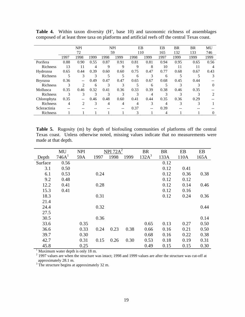
Table 4. Within taxon diversity (H’, base 10) and taxonomic richness of assemblages composed of at least three taxa on platforms and artificial reefs off the central Texas coast. NPI
72 NPI 59
EB 110
EB 165
BR 132
BR 133
MU 746
1997 1998 1999 1998 1999 1998 1999 1997 1999 1999 1999 Porifera 0.88 0.90 0.55 0.87 0.91 0.81 0.81 0.94 0.95 0.65 0.56
Richness 13 11 4 9 9 9 8 10 11 11 4 Hydrozoa 0.65 0.44 0.39 0.60 0.60 0.75 0.47 0.77 0.68 0.67 0.43
Richness 5 3 3 5 5 6 3 6 5 5 3 Bryozoa 0.36 -- 0.49 0.47 0.47 0.65 0.67 0.68 0.45 0.44 --
Richness 3 2 6 3 3 5 6 5 3 3 0 Mollusca 0.35 0.46 0.32 0.41 0.36 0.33 0.39 0.38 0.46 0.35 --
Richness 3 3 3 3 3 3 4 3 3 3 2 Chlorophyta 0.35 -- 0.46 0.48 0.60 0.41 0.44 0.35 0.36 0.29 --
Richness 4 2 3 4 4 4 3 4 3 3 1 Scleractinia -- -- -- -- -- 0.37 -- 0.39 -- -- --
Richness 1 1 1 1 1 3 1 4 1 1 0
Table 5. Rugosity (m) by depth of biofouling communities of platforms off the central Texas coast. Unless otherwise noted, missing values indicate that no measurements were made at that depth.
MU NPI NPI 72A2 BR BR EB EB
Depth 746A1 59A 1997 1998 1999 132A3 133A 110A 165A Surface 0.56 0.12
3.1 0.50 0.12 0.41 6.1 0.53 0.24 0.12 0.36 0.389.2 0.48 0.12 0.12
12.2 0.41 0.28 0.12 0.14 0.4615.3 0.41 0.12 0.16 18.3 0.31 0.12 0.24 0.3621.4 24.4 0.32 0.4427.5 30.5 0.36 0.1433.6 0.35 0.65 0.13 0.27 0.5036.6 0.33 0.24 0.23 0.38 0.66 0.16 0.21 0.5039.7 0.30 0.68 0.16 0.22 0.3842.7 0.31 0.15 0.26 0.30 0.53 0.18 0.19 0.3145.8 0.25 0.49 0.15 0.15 0.30
1 Maximum water depth is only 18 m. 2 1997 values are when the structure was intact; 1998 and 1999 values are after the structure was cut-off at approximately 28.1 m. 3 The structure begins at approximately 32 m.
19
60
Mol
lusc
a
9.0
Porif
era
4.5
Alga
e
4.0Hy
droz
oa0.6
Rugo
sity
(m)
0
6.1
12.2
18.3
24.4
Dep
th (m
)
% Cover
0 50 100% Similarity
Bray Curtis Cluster Analysis (Complete Link)6.1 m
12.2 m
18.3 m
24.4 m
30.5 m
ZONE I
ZONE II
0.42
0.78
0.27
0.14
0
Depth H’
60
Mol
lusc
a
9.0
Porif
era
4.5
Alga
e
4.0Hy
droz
oa0.6
Rugo
sity
(m)
0
6.1
12.2
18.3
24.4
Dep
th (m
)
% Cover
60
Mol
lusc
a
9.0
Porif
era
4.5
Alga
e
4.0Hy
droz
oa0.6
Rugo
sity
(m)
0
6.1
12.2
18.3
24.4
6.1
12.2
18.3
24.4
Dep
th (m
)
% Cover
0 50 100% Similarity0 50 100% Similarity
Bray Curtis Cluster Analysis (Complete Link)6.1 m
12.2 m
18.3 m
24.4 m
30.5 m
ZONE I
ZONE II
0.42
0.78
0.27
0.14
0
0.42
0.78
0.27
0.14
0
Depth H’
Fig. 15. Vertical zonation of biofouling communities on MU 746A determined using Bray-Curtis cluster analysis of community similarity. Note differing scales on taxa by depth diagram; taxa are arranged from highest to lowest percent cover.
20
3.1 m6.1 m9.2 m
12.2 m15.3 m18.3 m21.4 m24.4 m27.5 m30.5 m33.6 m36.6 m39.7 m42.7 m45.8 m48.8 m51.9 m
0.711.101.091.091.201.071.141.091.171.101.181.151.120.910.850.780.63
Depth H’Bray Curtis Cluster Analysis (Complete Link)
0 50 100% Similarity
Porif
era
4.5Hy
droz
oa
1.0
Bryo
zoa
1.2
Alga
e
18
Mol
lusc
a2.4
Cirri
pedi
a
0.33
Alcy
onar
ia
3.6
Rugo
sity
0.36
6.1
12.2
18.3
24.4
30.5
36.6
42.7
48.8
Dep
th (m
)
ZONE I
ZONE II
ZONE III
Percent Cover
NODATA
0
ZONE IV
3.1 m6.1 m9.2 m
12.2 m15.3 m18.3 m21.4 m24.4 m27.5 m30.5 m33.6 m36.6 m39.7 m42.7 m45.8 m48.8 m51.9 m
0.711.101.091.091.201.071.141.091.171.101.181.151.120.910.850.780.63
Depth H’
3.1 m6.1 m9.2 m
12.2 m15.3 m18.3 m21.4 m24.4 m27.5 m30.5 m33.6 m36.6 m39.7 m42.7 m45.8 m48.8 m51.9 m
3.1 m6.1 m9.2 m
12.2 m15.3 m18.3 m21.4 m24.4 m27.5 m30.5 m33.6 m36.6 m39.7 m42.7 m45.8 m48.8 m51.9 m
0.711.101.091.091.201.071.141.091.171.101.181.151.120.910.850.780.63
0.711.101.091.091.201.071.141.091.171.101.181.151.120.910.850.780.63
Depth H’Bray Curtis Cluster Analysis (Complete Link)
0 50 100% Similarity0 50 100% Similarity
Porif
era
4.5Hy
droz
oa
1.0
Bryo
zoa
1.2
Alga
e
18
Mol
lusc
a2.4
Cirri
pedi
a
0.33
Alcy
onar
ia
3.6
Rugo
sity
0.36
6.1
12.2
18.3
24.4
30.5
36.6
42.7
48.8
Dep
th (m
)
ZONE I
ZONE II
ZONE III
Percent Cover
NODATA
0
ZONE IV
Porif
era
4.5
Porif
era
4.5Hy
droz
oa
1.0Hy
droz
oa
1.0
Bryo
zoa
1.2
Bryo
zoa
1.2
Alga
e
18
Alga
e
18
Mol
lusc
a2.4
Mol
lusc
a2.4
Cirri
pedi
a
0.33
Cirri
pedi
a
0.33
Alcy
onar
ia
3.6
Alcy
onar
ia
3.6
Rugo
sity
0.360.36
6.1
12.2
18.3
24.4
30.5
36.6
42.7
48.8
6.1
12.2
18.3
24.4
30.5
36.6
42.7
48.8
Dep
th (m
)
ZONE I
ZONE II
ZONE III
Percent Cover
NODATA
0
ZONE IV
Fig. 16. Vertical zonation of biofouling communities on NPI 59A determined using Bray-Curtis cluster analysis of community similarity. Note differing scales on taxa by depth diagram; taxa are arranged from highest to lowest percent cover.
21
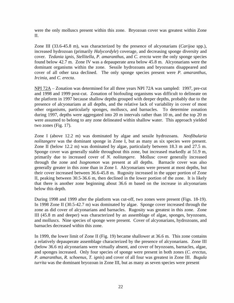
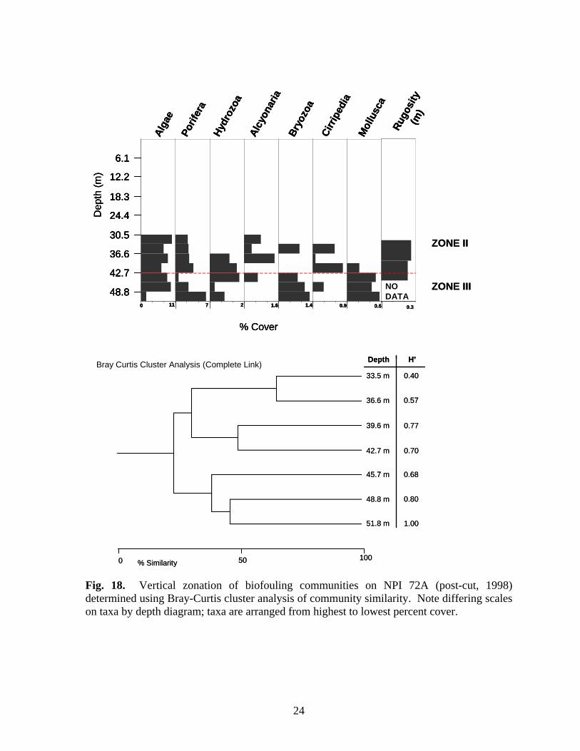
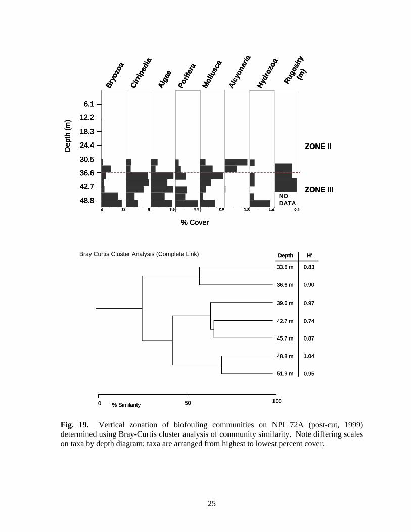
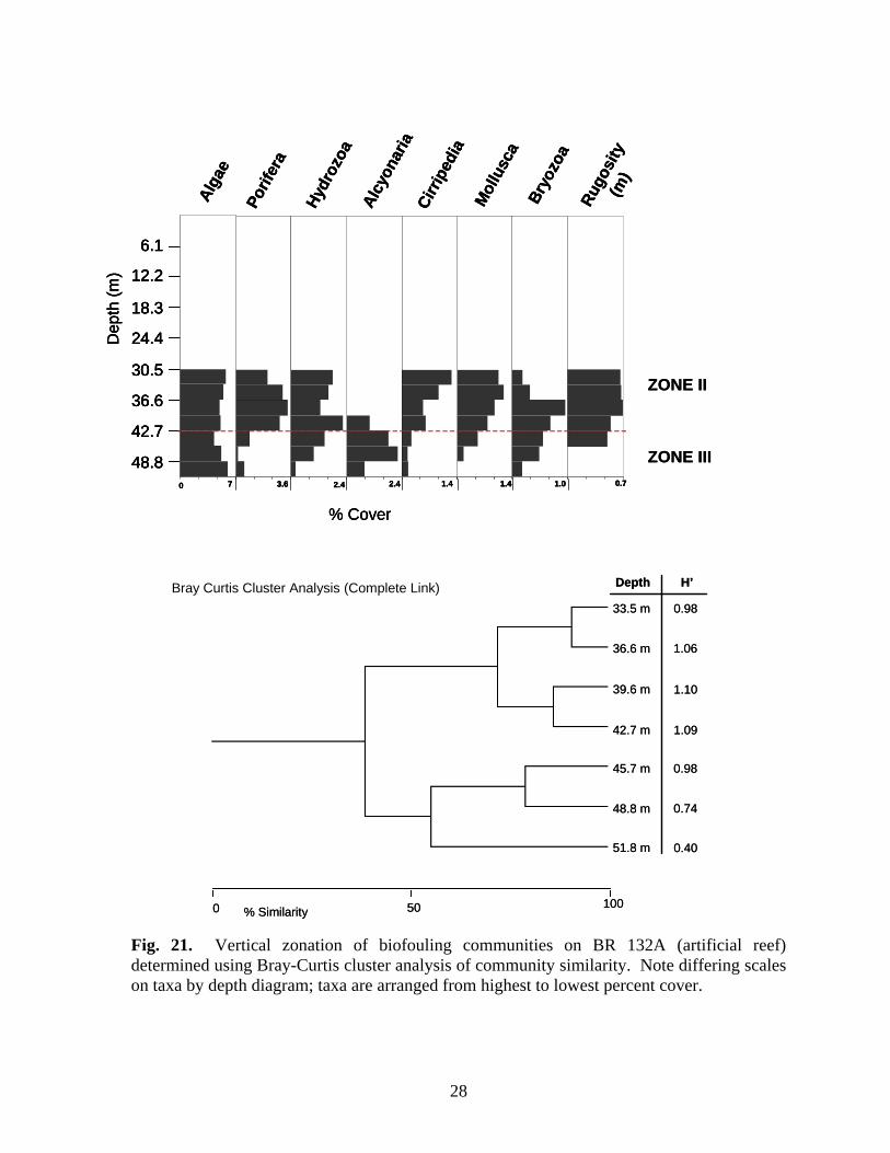
were the only molluscs present within this zone. Bryozoan cover was greatest within Zone II. Zone III (33.6-45.8 m), was characterized by the presence of alcyonarians (Carijoa spp.), increased hydrozoan (primarily Halycordyle) coverage, and decreasing sponge diversity and cover. Tedania ignis, Stellitella, P. amaranthus, and C. erecta were the only sponge species found below 42.7 m. Zone IV was a depauperate area below 45.8 m. Alcyonarians were the dominant organisms within the zone. Sessile hydrozoans and bryozoans disappeared and cover of all other taxa declined. The only sponge species present were P. amaranthus, Ircinia, and C. erecta. NPI 72A – Zonation was determined for all three years NPI 72A was sampled: 1997, pre-cut and 1998 and 1999 post-cut. Zonation of biofouling organisms was difficult to delineate on the platform in 1997 because shallow depths grouped with deeper depths, probably due to the presence of alcyonarians at all depths, and the relative lack of variability in cover of most other organisms, particularly sponges, molluscs, and barnacles. To determine zonation during 1997, depths were aggregated into 20 m intervals rather than 10 m, and the top 20 m were assumed to belong to any zone delineated within shallow water. This approach yielded two zones (Fig. 17). Zone I (above 12.2 m) was dominated by algae and sessile hydrozoans. Neofibularia nolitangere was the dominant sponge in Zone I, but as many as six species were present. Zone II (below 12.2 m) was dominated by algae, particularly between 18.3 m and 27.5 m. Sponge cover was generally stable throughout this zone, but increased markedly at 51.9 m, primarily due to increased cover of N. nolitangere. Mollusc cover generally increased through the zone and Isognomon was present at all depths. Barnacle cover was also generally greater in this zone than in Zone I. Alcyonarians were present at most depths, but their cover increased between 36.6-45.8 m. Rugosity increased in the upper portion of Zone II, peaking between 30.5-36.6 m, then declined in the lower portion of the zone. It is likely that there is another zone beginning about 36.6 m based on the increase in alcyonarians below this depth. During 1998 and 1999 after the platform was cut-off, two zones were present (Figs. 18-19). In 1998 Zone II (30.5-42.7 m) was dominated by algae. Sponge cover increased through the zone as did cover of alcyonarians and barnacles. Rugosity was greatest in this zone. Zone III (45.8 m and deeper) was characterized by an assemblage of algae, sponges, bryozoans, and molluscs. Nine species of sponge were present. Cover of alcyonarians, hydrozoans, and barnacles decreased within this zone. In 1999, the lower limit of Zone II (Fig. 19) became shallower at 36.6 m. This zone contains a relatively depauperate assemblage characterized by the presence of alcyonarians. Zone III (below 36.6 m) alcyonarians were virtually absent, and cover of bryozoans, barnacles, algae, and sponges increased. Only four species of sponge were present in both zones (C. erectus, P. amaranthus, R. schoenus, T. ignis) and cover of all four was greatest in Zone III. Bugula turrita was the dominant bryozoan in Zone III, but as many as seven species were present
22
Rugo
sity
(m)
Hydr
ozoa
Bryo
zoa
Alga
e
Cirri
pedi
a
Alcy
onar
iaM
ollu
sca
Porif
era
6.0 4.5 1.01.2 0.7 0.45 0.3 0.4
6.1
12.2
18.3
24.4
30.5
36.6
42.7
48.8
% Cover
Dep
th (m
)
0 50 100% Similarity
Bray Curtis Cluster Analysis (Complete Link)12.2 m
18.3 m
36.6 m
42.7 m
30.5 m
24.4 m
48.8 m
0.74
0.90
1.02
1.08
0.95
0.75
1.14
Depth H’
ZONE I
ZONE II
Rugo
sity
(m)
Hydr
ozoa
Bryo
zoa
Alga
e
Cirri
pedi
a
Alcy
onar
iaM
ollu
sca
Porif
era
6.0 4.5 1.01.2 0.7 0.45 0.3 0.4
6.1
12.2
18.3
24.4
30.5
36.6
42.7
48.8
% Cover
Dep
th (m
)
Rugo
sity
(m)
Hydr
ozoa
Bryo
zoa
Alga
e
Cirri
pedi
a
Alcy
onar
iaM
ollu
sca
Porif
era
Rugo
sity
(m)
Hydr
ozoa
Bryo
zoa
Alga
e
Cirri
pedi
a
Alcy
onar
iaM
ollu
sca
Porif
era
6.0 4.5 1.01.2 0.7 0.45 0.3 0.4
6.1
12.2
18.3
24.4
30.5
36.6
42.7
48.8
6.1
12.2
18.3
24.4
30.5
36.6
42.7
48.8
% Cover
Dep
th (m
)
0 50 100% Similarity
Bray Curtis Cluster Analysis (Complete Link)12.2 m
18.3 m
36.6 m
42.7 m
30.5 m
24.4 m
48.8 m
0.74
0.90
1.02
1.08
0.95
0.75
1.14
Depth H’
0 50 100% Similarity
Bray Curtis Cluster Analysis (Complete Link)12.2 m
18.3 m
36.6 m
42.7 m
30.5 m
24.4 m
48.8 m
0.74
0.90
1.02
1.08
0.95
0.75
1.14
Depth H’
12.2 m
18.3 m
36.6 m
42.7 m
30.5 m
24.4 m
48.8 m
0.74
0.90
1.02
1.08
0.95
0.75
1.14
Depth H’
ZONE I
ZONE II
Fig. 17. Vertical zonation of biofouling communities on NPI 72A (pre-cut, 1997) determined using Bray-Curtis cluster analysis of community similarity. Note differing scales on taxa by depth diagram; taxa are arranged from highest to lowest percent cover.
23
11 7 2 1.6 1.4 0.9 0.6 0.3
6.1
12.2
18.3
24.4
30.5
36.6
42.7
48.8
Dep
th (m
)
% Cover
Rugo
sity
(m)
Hydr
ozoa
Bryo
zoa
Alga
e
Cirri
pedi
a
Alcy
onar
ia
Mol
lusc
a
Porif
era
0
Bray Curtis Cluster Analysis (Complete Link)
0 50 100% Similarity
33.5 m
36.6 m
39.6 m
42.7 m
45.7 m
48.8 m
51.8 m
0.40
0.57
0.77
0.70
0.68
0.80
1.00
Depth H’
ZONE II
ZONE IIINODATA
11 7 2 1.6 1.4 0.9 0.6 0.3
6.1
12.2
18.3
24.4
30.5
36.6
42.7
48.8
Dep
th (m
)
% Cover
Rugo
sity
(m)
Hydr
ozoa
Bryo
zoa
Alga
e
Cirri
pedi
a
Alcy
onar
ia
Mol
lusc
a
Porif
era
0 11 7 2 1.6 1.4 0.9 0.6 0.3
6.1
12.2
18.3
24.4
30.5
36.6
42.7
48.8
6.1
12.2
18.3
24.4
30.5
36.6
42.7
48.8
Dep
th (m
)
% Cover
Rugo
sity
(m)
Hydr
ozoa
Bryo
zoa
Alga
e
Cirri
pedi
a
Alcy
onar
ia
Mol
lusc
a
Porif
era
0
Bray Curtis Cluster Analysis (Complete Link)
0 50 100% Similarity
33.5 m
36.6 m
39.6 m
42.7 m
45.7 m
48.8 m
51.8 m
0.40
0.57
0.77
0.70
0.68
0.80
1.00
Depth H’Bray Curtis Cluster Analysis (Complete Link)
0 50 100% Similarity0 50 100% Similarity
33.5 m
36.6 m
39.6 m
42.7 m
45.7 m
48.8 m
51.8 m
0.40
0.57
0.77
0.70
0.68
0.80
1.00
Depth H’
33.5 m
36.6 m
39.6 m
42.7 m
45.7 m
48.8 m
51.8 m
0.40
0.57
0.77
0.70
0.68
0.80
1.00
Depth H’
ZONE II
ZONE IIINODATA
Fig. 18. Vertical zonation of biofouling communities on NPI 72A (post-cut, 1998) determined using Bray-Curtis cluster analysis of community similarity. Note differing scales on taxa by depth diagram; taxa are arranged from highest to lowest percent cover.
24
Alcy
onar
ia
0 50 100% Similarity
Bray Curtis Cluster Analysis (Complete Link)
33.5 m
36.6 m
39.6 m
42.7 m
45.7 m
48.8 m
51.9 m
0.83
0.90
0.97
0.74
0.87
1.04
0.95
Depth H’
12 8 3.5 3.3 1.42.0 1.8 0.4
6.1
12.2
18.3
24.4
30.5
36.6
42.7
48.8
Dep
th (m
)
% Cover
Rugo
sity
(m)
Hydr
ozoa
Bryo
zoa
Alga
e
Cirri
pedi
a
Mol
lusc
a
Porif
era
ZONE II
ZONE III
0
NODATA
Alcy
onar
ia
0 50 100% Similarity0 50 100% Similarity
Bray Curtis Cluster Analysis (Complete Link)
33.5 m
36.6 m
39.6 m
42.7 m
45.7 m
48.8 m
51.9 m
0.83
0.90
0.97
0.74
0.87
1.04
0.95
Depth H’
33.5 m
36.6 m
39.6 m
42.7 m
45.7 m
48.8 m
51.9 m
0.83
0.90
0.97
0.74
0.87
1.04
0.95
Depth H’
12 8 3.5 3.3 1.42.0 1.8 0.4
6.1
12.2
18.3
24.4
30.5
36.6
42.7
48.8
Dep
th (m
)
% Cover
Rugo
sity
(m)
Hydr
ozoa
Bryo
zoa
Alga
e
Cirri
pedi
a
Mol
lusc
a
Porif
era
ZONE II
ZONE III
0 12 8 3.5 3.3 1.42.0 1.8 0.4
6.1
12.2
18.3
24.4
30.5
36.6
42.7
48.8
6.1
12.2
18.3
24.4
30.5
36.6
42.7
48.8
Dep
th (m
)
% Cover
Rugo
sity
(m)
Hydr
ozoa
Bryo
zoa
Alga
e
Cirri
pedi
a
Mol
lusc
a
Porif
era
ZONE II
ZONE III
0
NODATA
Fig. 19. Vertical zonation of biofouling communities on NPI 72A (post-cut, 1999) determined using Bray-Curtis cluster analysis of community similarity. Note differing scales on taxa by depth diagram; taxa are arranged from highest to lowest percent cover.
25
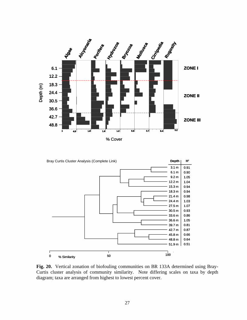
within the zone. The molluscan assemblage was dominated by P. colymbus. Isognomon was not noted in photo-transects on the structure in 1999. BR 133A – Three vertical zones were delineated on BR 133A (Fig. 20). Zone I (above 15.3 m) was dominated by algae. Cover of bryozoans, molluscs, and barnacles was generally greater within this zone. The sponges Pseudocertina sp., and P. amaranthus were found only in this zone, along with T. ignis. Isognomon was the dominant mollusc, and was found only within Zone I. Zone II (18.3-39.7 m) was characterized by generally decreasing algal cover and increasing cover of sponges. Tedania ignis was the dominant sponge species, but as many as six species were found within the zone. Molluscan cover decreased in the upper portion of the zone before disappearing below 33.5 m. Spondylus americanus and ark shells (Arcidae) were the only molluscs present within Zone II. Barnacle cover was relatively stable throughout the zone, and cover of both sessile hydrozoans and bryozoans was variable. A few alcyonarians were present between 27.5-33.6 m. Increased alcyonarian cover characterizes Zone III (below 39.7 m). Algal cover increases slightly within this zone, but most other taxa either decline in coverage or disappear altogether. Rugosity was greatest in Zone III. BR 132A (artificial reef) – Two vertical zones were delineated on this toppled platform (Fig. 21). Zone II (30.5-42.7 m) was characterized algae, a diverse assemblage of sponges (11 species), and sessile hydrozoans. Tedania ignis was the dominant sponge. Molluscan and barnacle cover was greatest in the upper portion of this zone and declined with depth. Rugosity was greatest in this zone. Zone III (45.8 m and below) was characterized by decreased cover or disappearance of most taxa and increased cover of alcyonarians. Tedania ignis was also the dominant sponge in this zone, and the only species found deeper than 48.8 m. Algal cover decreased slightly in the upper portion of this zone then increased in the lower portion. EB 110A – Four zones were characterized at EB 110 (Fig. 22). Zone I (above 6.1 m) was dominated by algae, molluscs, and barnacles. Isognomon was the dominant mollusc in this zone and was only present in this zone and the top 3.1 m of Zone II. Although sponge cover was relatively low in Zone I, the assemblage was diverse with six species. Rugosity was greatest in Zone I. Marked declines in cover of algae, molluscs, and barnacles, and increasing cover of sponges, bryozoans, and sessile hydrozoans characterized Zone II (9.2-21.3 m). A diverse assemblage of sponges (8 species) was present dominated by T. ignis. Bryozoan cover was greatest in this zone, particularly between 9.2-15.3 m. Sponge cover continued to increase through Zone III (24.4-45.8 m) but there was no increase in the number of species present. Tedania ignis, N. notolitangere, and Helisarca sp. were the dominant sponges. Cover of algae, molluscs and barnacles changed little from that seen in
26
Porif
era
1.6 1.2
Hydr
ozoa
Bryo
zoa
0.84.5
Alga
e
0.7
Mol
lusc
a
0.4
Cirri
pedi
a
1.8
Alcy
onar
ia
0.2
Rugo
sity
6.1
12.2
18.3
24.4
30.5
36.6
42.7
48.8
Dep
th (m
)
ZONE I
ZONE II
ZONE III
% Cover
0 50 100% Similarity
Bray Curtis Cluster Analysis (Complete Link)
3.1 m6.1 m9.2 m
12.2 m15.3 m18.3 m21.4 m24.4 m27.5 m30.5 m33.6 m36.6 m39.7 m42.7 m45.8 m48.8 m51.9 m
0.910.901.051.040.940.940.981.031.070.930.861.050.810.870.660.640.51
Depth H’
0 50 100% Similarity
0
Porif
era
1.6 1.2
Hydr
ozoa
Bryo
zoa
0.84.5
Alga
e
0.7
Mol
lusc
a
0.4
Cirri
pedi
a
1.8
Alcy
onar
ia
0.2
Rugo
sity
6.1
12.2
18.3
24.4
30.5
36.6
42.7
48.8
Dep
th (m
)
ZONE I
ZONE II
ZONE III
Porif
era
1.6
Porif
era
1.6 1.2
Hydr
ozoa
1.2
Hydr
ozoa
Bryo
zoa
0.8
Bryo
zoa
0.84.5
Alga
e
4.5
Alga
e
0.7
Mol
lusc
a
0.7
Mol
lusc
a
0.4
Cirri
pedi
a
0.4
Cirri
pedi
a
1.8
Alcy
onar
ia
1.8
Alcy
onar
ia
0.2
Rugo
sity
0.2
Rugo
sity
6.1
12.2
18.3
24.4
30.5
36.6
42.7
48.8
6.1
12.2
18.3
24.4
30.5
36.6
42.7
48.8
Dep
th (m
)
ZONE I
ZONE II
ZONE III
% Cover
0 50 100% Similarity
Bray Curtis Cluster Analysis (Complete Link)
3.1 m6.1 m9.2 m
12.2 m15.3 m18.3 m21.4 m24.4 m27.5 m30.5 m33.6 m36.6 m39.7 m42.7 m45.8 m48.8 m51.9 m
0.910.901.051.040.940.940.981.031.070.930.861.050.810.870.660.640.51
Depth H’
0 50 100% Similarity
0 50 100% Similarity0 50 100% Similarity
Bray Curtis Cluster Analysis (Complete Link)
3.1 m6.1 m9.2 m
12.2 m15.3 m18.3 m21.4 m24.4 m27.5 m30.5 m33.6 m36.6 m39.7 m42.7 m45.8 m48.8 m51.9 m
0.910.901.051.040.940.940.981.031.070.930.861.050.810.870.660.640.51
Depth H’
3.1 m6.1 m9.2 m
12.2 m15.3 m18.3 m21.4 m24.4 m27.5 m30.5 m33.6 m36.6 m39.7 m42.7 m45.8 m48.8 m51.9 m
3.1 m6.1 m9.2 m
12.2 m15.3 m18.3 m21.4 m24.4 m27.5 m30.5 m33.6 m36.6 m39.7 m42.7 m45.8 m48.8 m51.9 m
0.910.901.051.040.940.940.981.031.070.930.861.050.810.870.660.640.51
0.910.901.051.040.940.940.981.031.070.930.861.050.810.870.660.640.51
Depth H’
0 50 100% Similarity0 50 100% Similarity
0
Fig. 20. Vertical zonation of biofouling communities on BR 133A determined using Bray-Curtis cluster analysis of community similarity. Note differing scales on taxa by depth diagram; taxa are arranged from highest to lowest percent cover.
27
Porif
era
3.6 2.4
Hydr
ozoa
2.4
Alcy
onar
ia
Mol
lusc
a0
6.1
12.2
18.3
24.4
30.5
36.6
42.7
48.8
Dep
th (m
)
% Cover
1.4
Cirri
pedi
a1.4
Bryo
zoa
1.0 0.7
Rugo
sity
(m)
7
Alga
e
Bray Curtis Cluster Analysis (Complete Link)
0 50 100% Similarity
33.5 m
36.6 m
39.6 m
42.7 m
45.7 m
48.8 m
51.8 m
0.98
1.06
1.10
1.09
0.98
0.74
0.40
Depth H’
ZONE II
ZONE III
Porif
era
3.6 2.4
Hydr
ozoa
2.4
Alcy
onar
ia
Mol
lusc
a0
6.1
12.2
18.3
24.4
30.5
36.6
42.7
48.8
Dep
th (m
)
% Cover
1.4
Cirri
pedi
a1.4
Bryo
zoa
1.0 0.7
Rugo
sity
(m)
7
Alga
e
Porif
era
3.6 2.4
Hydr
ozoa
2.4
Alcy
onar
ia
Mol
lusc
a0
6.1
12.2
18.3
24.4
30.5
36.6
42.7
48.8
6.1
12.2
18.3
24.4
30.5
36.6
42.7
48.8
Dep
th (m
)
% Cover
1.41.4
Cirri
pedi
a1.4
Bryo
zoa
1.0 0.7
Rugo
sity
(m)
7
Alga
e
Bray Curtis Cluster Analysis (Complete Link)
0 50 100% Similarity
33.5 m
36.6 m
39.6 m
42.7 m
45.7 m
48.8 m
51.8 m
0.98
1.06
1.10
1.09
0.98
0.74
0.40
Depth H’Bray Curtis Cluster Analysis (Complete Link)
0 50 100% Similarity0 50 100% Similarity
33.5 m
36.6 m
39.6 m
42.7 m
45.7 m
48.8 m
51.8 m
0.98
1.06
1.10
1.09
0.98
0.74
0.40
Depth H’
33.5 m
36.6 m
39.6 m
42.7 m
45.7 m
48.8 m
51.8 m
0.98
1.06
1.10
1.09
0.98
0.74
0.40
Depth H’
ZONE II
ZONE III
Fig. 21. Vertical zonation of biofouling communities on BR 132A (artificial reef) determined using Bray-Curtis cluster analysis of community similarity. Note differing scales on taxa by depth diagram; taxa are arranged from highest to lowest percent cover.
28

Alcy
onar
ia3 0.84.24.2 3.5 2 0.9 0.45
NODATA
6.1
12.2
18.3
24.4
30.5
36.6
42.7
48.8
Dep
th (m
)
% Cover
Rugo
sity
(m)
Hydr
ozoa
Bryo
zoa
Alga
e
Cirri
pedi
a
Mol
lusc
a
Porif
era
0
Bray Curtis Cluster Analysis (Complete Link)
0 50 100% Similarity
45.8 m42.7 m39.7 m
30.5 m27.5 m24.4 m21.4 m18.3 m
3.1 m 0.616.1 m 0.969.2 m 1.19
12.2 m 1.2115.3 m 1.20
1.271.281.37
1.2833.6 m 1.2136.6 m 1.30
1.231.26
1.32
1.2548.8 m 1.1651.9 m 1.09
Depth H’
ZONE I
ZONE II
ZONE III
ZONE IV
Alcy
onar
ia3 0.84.24.2 3.5 2 0.9 0.45
NODATA
6.1
12.2
18.3
24.4
30.5
36.6
42.7
48.8
Dep
th (m
)
% Cover
Rugo
sity
(m)
Hydr
ozoa
Bryo
zoa
Alga
e
Cirri
pedi
a
Mol
lusc
a
Porif
era
0 3 0.84.24.2 3.5 2 0.9 0.45
NODATA
6.1
12.2
18.3
24.4
30.5
36.6
42.7
48.8
6.1
12.2
18.3
24.4
30.5
36.6
42.7
48.8
Dep
th (m
)
% Cover
Rugo
sity
(m)
Hydr
ozoa
Bryo
zoa
Alga
e
Cirri
pedi
a
Mol
lusc
a
Porif
era
0
Bray Curtis Cluster Analysis (Complete Link)
0 50 100% Similarity
45.8 m42.7 m39.7 m
30.5 m27.5 m24.4 m21.4 m18.3 m
3.1 m 0.616.1 m 0.969.2 m 1.19
12.2 m 1.2115.3 m 1.20
1.271.281.37
1.2833.6 m 1.2136.6 m 1.30
1.231.26
1.32
1.2548.8 m 1.1651.9 m 1.09
Depth H’Bray Curtis Cluster Analysis (Complete Link)
0 50 100% Similarity0 50 100% Similarity
45.8 m42.7 m39.7 m
30.5 m27.5 m24.4 m21.4 m18.3 m
3.1 m 0.616.1 m 0.969.2 m 1.19
12.2 m 1.2115.3 m 1.20
1.271.281.37
1.2833.6 m 1.2136.6 m 1.30
1.231.26
1.32
1.2548.8 m 1.1651.9 m 1.09
Depth H’
45.8 m42.7 m39.7 m
30.5 m27.5 m24.4 m21.4 m18.3 m
3.1 m 0.613.1 m 0.616.1 m 0.966.1 m 0.969.2 m 1.199.2 m 1.19
12.2 m 1.2112.2 m 1.2115.3 m 1.2015.3 m 1.20
1.271.281.37
1.2833.6 m 1.2133.6 m 1.2136.6 m 1.3036.6 m 1.30
1.231.26
1.32
1.2548.8 m 1.1648.8 m 1.1651.9 m 1.0951.9 m 1.09
Depth H’Depth H’
ZONE I
ZONE II
ZONE III
ZONE IV
Fig. 22. Vertical zonation of biofouling communities on EB 110A determined using Bray-Curtis cluster analysis of community similarity. Note differing scales on taxa by depth diagram; taxa are arranged from highest to lowest percent cover.
29
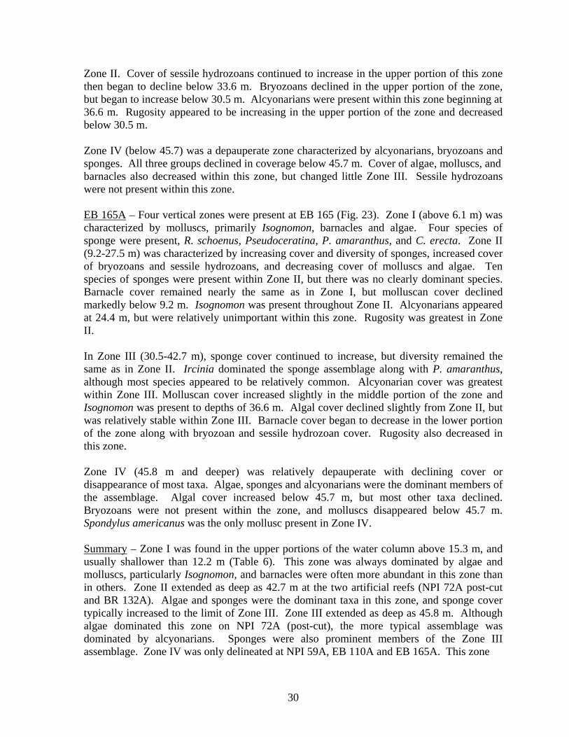
Zone II. Cover of sessile hydrozoans continued to increase in the upper portion of this zone then began to decline below 33.6 m. Bryozoans declined in the upper portion of the zone, but began to increase below 30.5 m. Alcyonarians were present within this zone beginning at 36.6 m. Rugosity appeared to be increasing in the upper portion of the zone and decreased below 30.5 m. Zone IV (below 45.7) was a depauperate zone characterized by alcyonarians, bryozoans and sponges. All three groups declined in coverage below 45.7 m. Cover of algae, molluscs, and barnacles also decreased within this zone, but changed little Zone III. Sessile hydrozoans were not present within this zone. EB 165A – Four vertical zones were present at EB 165 (Fig. 23). Zone I (above 6.1 m) was characterized by molluscs, primarily Isognomon, barnacles and algae. Four species of sponge were present, R. schoenus, Pseudoceratina, P. amaranthus, and C. erecta. Zone II (9.2-27.5 m) was characterized by increasing cover and diversity of sponges, increased cover of bryozoans and sessile hydrozoans, and decreasing cover of molluscs and algae. Ten species of sponges were present within Zone II, but there was no clearly dominant species. Barnacle cover remained nearly the same as in Zone I, but molluscan cover declined markedly below 9.2 m. Isognomon was present throughout Zone II. Alcyonarians appeared at 24.4 m, but were relatively unimportant within this zone. Rugosity was greatest in Zone II. In Zone III (30.5-42.7 m), sponge cover continued to increase, but diversity remained the same as in Zone II. Ircinia dominated the sponge assemblage along with P. amaranthus, although most species appeared to be relatively common. Alcyonarian cover was greatest within Zone III. Molluscan cover increased slightly in the middle portion of the zone and Isognomon was present to depths of 36.6 m. Algal cover declined slightly from Zone II, but was relatively stable within Zone III. Barnacle cover began to decrease in the lower portion of the zone along with bryozoan and sessile hydrozoan cover. Rugosity also decreased in this zone. Zone IV (45.8 m and deeper) was relatively depauperate with declining cover or disappearance of most taxa. Algae, sponges and alcyonarians were the dominant members of the assemblage. Algal cover increased below 45.7 m, but most other taxa declined. Bryozoans were not present within the zone, and molluscs disappeared below 45.7 m. Spondylus americanus was the only mollusc present in Zone IV. Summary – Zone I was found in the upper portions of the water column above 15.3 m, and usually shallower than 12.2 m (Table 6). This zone was always dominated by algae and molluscs, particularly Isognomon, and barnacles were often more abundant in this zone than in others. Zone II extended as deep as 42.7 m at the two artificial reefs (NPI 72A post-cut and BR 132A). Algae and sponges were the dominant taxa in this zone, and sponge cover typically increased to the limit of Zone III. Zone III extended as deep as 45.8 m. Although algae dominated this zone on NPI 72A (post-cut), the more typical assemblage was dominated by alcyonarians. Sponges were also prominent members of the Zone III assemblage. Zone IV was only delineated at NPI 59A, EB 110A and EB 165A. This zone
30
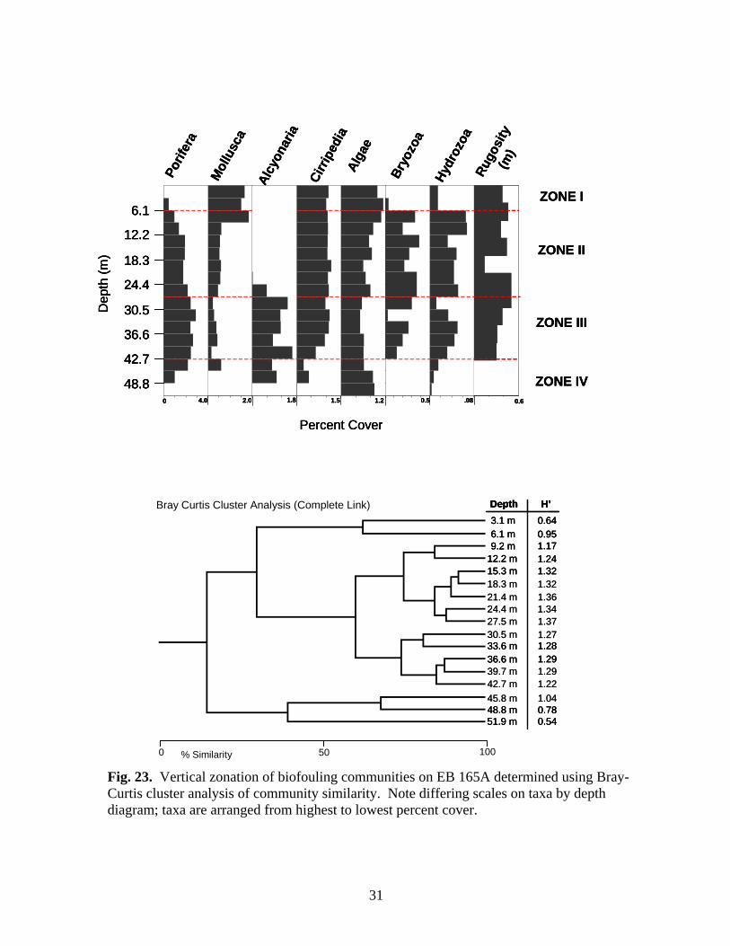
45.8 m42.7 m39.7 m
30.5 m27.5 m24.4 m21.4 m18.3 m
3.1 m 0.646.1 m 0.959.2 m 1.17
12.2 m 1.2415.3 m 1.32
1.321.361.34
1.2733.6 m 1.2836.6 m 1.29
1.221.29
1.37
1.0448.8 m 0.7851.9 m 0.54
Depth H’
0 50 100% Similarity
Bray Curtis Cluster Analysis (Complete Link)
Rugo
sity
(m)
0.60
Cirri
pedi
a
1.52.0
Mol
lusc
a
4.0
Porif
era
Hydr
ozoa
.080.5Br
yozo
a
6.1
12.2
18.3
24.4
30.5
36.6
42.7
48.8
Dep
th (m
)
ZONE I
ZONE II
ZONE III
Alcy
onar
ia
1.8
Alga
e
1.2
ZONE IV
Percent Cover
45.8 m42.7 m39.7 m
30.5 m27.5 m24.4 m21.4 m18.3 m
3.1 m 0.646.1 m 0.959.2 m 1.17
12.2 m 1.2415.3 m 1.32
1.321.361.34
1.2733.6 m 1.2836.6 m 1.29
1.221.29
1.37
1.0448.8 m 0.7851.9 m 0.54
Depth H’
45.8 m42.7 m39.7 m
30.5 m27.5 m24.4 m21.4 m18.3 m
3.1 m 0.646.1 m 0.959.2 m 1.17
12.2 m 1.2415.3 m 1.32
1.321.361.34
1.2733.6 m 1.2836.6 m 1.29
1.221.29
1.37
1.0448.8 m 0.7851.9 m 0.54
Depth H’
45.8 m42.7 m39.7 m
30.5 m27.5 m24.4 m21.4 m18.3 m
3.1 m 0.643.1 m 0.646.1 m 0.956.1 m 0.959.2 m 1.179.2 m 1.17
12.2 m 1.2412.2 m 1.2415.3 m 1.3215.3 m 1.32
1.321.361.34
1.2733.6 m 1.2833.6 m 1.2836.6 m 1.2936.6 m 1.29
1.221.29
1.37
1.0448.8 m 0.7848.8 m 0.7851.9 m 0.5451.9 m 0.54
Depth H’Depth H’
0 50 100% Similarity0 50 100% Similarity
Bray Curtis Cluster Analysis (Complete Link)
Rugo
sity
(m)
0.60
Cirri
pedi
a
1.52.0
Mol
lusc
a
4.0
Porif
era
Hydr
ozoa
.080.5Br
yozo
a
6.1
12.2
18.3
24.4
30.5
36.6
42.7
48.8
Dep
th (m
)
ZONE I
ZONE II
ZONE III
Alcy
onar
ia
1.8
Alga
e
1.2
ZONE IV
Percent Cover
Rugo
sity
(m)
0.60
Cirri
pedi
a
1.52.0
Mol
lusc
a
4.0
Porif
era
Hydr
ozoa
.080.5Br
yozo
a
6.1
12.2
18.3
24.4
30.5
36.6
42.7
48.8
6.1
12.2
18.3
24.4
30.5
36.6
42.7
48.8
Dep
th (m
)
ZONE I
ZONE II
ZONE III
Alcy
onar
ia
1.8
Alga
e
1.2
ZONE IV
Percent Cover
Fig. 23. Vertical zonation of biofouling communities on EB 165A determined using Bray-Curtis cluster analysis of community similarity. Note differing scales on taxa by depth diagram; taxa are arranged from highest to lowest percent cover.
31
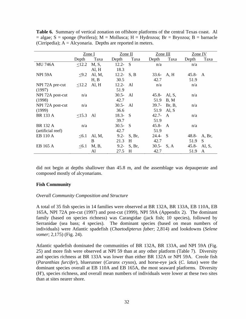
Table 6. Summary of vertical zonation on offshore platforms of the central Texas coast. Al = algae; S = sponge (Porifera); M = Mollusca; H = Hydrozoa; Br = Bryozoa; B = barnacle (Cirripedia); A = Alcyonaria. Depths are reported in meters.
Zone I Zone II Zone III Zone IV
Depth Taxa Depth Taxa Depth Taxa Depth Taxa MU 746A <12.2 M, S,
Al, H 12.2-18.3
S n/a n/a
NPI 59A <9.2 Al, M, H, B
12.2-30.5
S, B 33.6-42.7
A, H 45.8-51.9
A
NPI 72A pre-cut (1997)
<12.2 Al, H 12.2-51.9
Al n/a n/a
NPI 72A post-cut (1998)
n/a 30.5-42.7
Al 45.8-51.9
Al, S, B, M
n/a
NPI 72A post-cut (1999)
n/a 30.5-36.6
Al 39.7-51.9
Br, B, Al, S
n/a
BR 133 A <15.3 Al 18.3-39.7
S 42.7-51.9
A n/a
BR 132 A (artificial reef)
n/a 30.5-42.7
S 45.8-51.9
A n/a
EB 110 A <6.1 Al, M, B
9.2-21.3
S, Br, H
24.4-42.7
S 48.8-51.9
A, Br, S
EB 165 A <6.1 M, B, Al
9.2-27.5
S, Br, H
30.5-42.7
S, A 45.8-51.9
Al, S, A
did not begin at depths shallower than 45.8 m, and the assemblage was depauperate and composed mostly of alcyonarians. Fish Community Overall Community Composition and Structure A total of 35 fish species in 14 families were observed at BR 132A, BR 133A, EB 110A, EB 165A, NPI 72A pre-cut (1997) and post-cut (1999), NPI 59A (Appendix 2). The dominant family (based on species richness) was Carangidae (jack fish; 10 species), followed by Serranidae (sea bass; 4 species). The dominant species (based on mean numbers of individuals) were Atlantic spadefish (Chaetodipterus faber; 2,814) and lookdowns (Selene vomer; 2,175) (Fig. 24). Atlantic spadefish dominated the communities of BR 132A, BR 133A, and NPI 59A (Fig. 25) and more fish were observed at NPI 59 than at any other platform (Table 7). Diversity and species richness at BR 133A was lower than either BR 132A or NPI 59A. Creole fish (Paranthias furcifer), bluerunner (Caranx crysos), and horse-eye jack (C. latus) were the dominant species overall at EB 110A and EB 165A, the most seaward platforms. Diversity (H'), species richness, and overall mean numbers of individuals were lower at these two sites than at sites nearer shore.
32
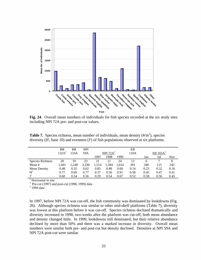
0
500
1000
1500
2000
2500
3000
Mea
n N
o. o
f Ind
ivid
uals
Creole fish
Creole wrasse
Amber jack
Crevalle jack
Gray snapper
Great barracuda
Spanish hogfish
Atlantic spadefish
Blue runner
Sergeant major
Bermuda chub
Vermillion snapper
Horse-eye jack
Rainbow runner
Spotfin hogfish
Lookdown
Atlantic bonito
Other
Fish
Fig. 24. Overall mean numbers of individuals for fish species recorded at the six study sites including NPI 72A pre- and post-cut values. Table 7. Species richness, mean number of individuals, mean density (#/m3), species diversity (H', base 10) and evenness (J') of fish populations observed at six platforms.
BR 132A1
BR 133A
NPI 59A
NPI 72A2
EB 110A
EB 165A3
1 Horizontal in situ
1997 1998 1999 Jan Jul Nov Species Richness 20 19 23 21 11 24 13 6 7 8 Mean # 1,041 1,248 3,336 1,514 1,584 1,614 391 346 115 242 Mean Density 0.48 0.35 0.62 0.83 0.88 0.60 0.14 0.23 0.32 0.16 H’ 0.77 0.69 0.77 0.37 0.56 0.91 0.58 0.45 0.47 0.41 J’ 0.60 0.54 0.56 0.29 0.54 0.67 0.52 0.58 0.56 0.45
2 Pre-cut (1997) and post-cut (1998, 1999) data 3 1994 data In 1997, before NPI 72A was cut-off, the fish community was dominated by lookdowns (Fig. 26). Although species richness was similar to other mid-shelf platforms (Table 7), diversity was lowest at this platform before it was cut-off. Species richness declined dramatically and diversity increased in 1998, two-weeks after the platform was cut-off; both mean abundance and density changed little. In 1999, lookdowns still dominated, but their relative abundance declined by more than 50% and there was a marked increase in diversity. Overall mean numbers were similar both pre- and post-cut but density declined. Densities at NPI 59A and NPI 72A post-cut were similar.
33
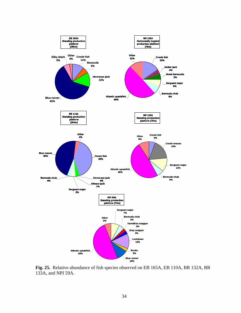
Silky shark5%
Other3%
Creole fish11%
Baracuda6%
Horeseye jack13%
Blue runner62%
EB 165AStanding production
platform(260m)
BR 132AHorizontally toppledproduction platform
(75m)
Atlantic spadefish49%
Bermuda chub8%
Sergeant major6%
Great barracuda5%
Amber jack4%
Creole fish16%
Other12%
Other4%
Creole fish39%
Blue runner46%
Horse-eye jack4%
Almaco jack1%
Sergeant major2%
Bermuda chub4%
EB 110AStanding production
platform(204m)
Atlantic spadefish49%
Bermuda chub6%
Sergeant major12%
Creole wrasse18%
Creole fish6%
Other9%
BR 133AStanding production
platform (75m)
NPI 59AStanding production
platform (74m)
Gray snapper3%
Vermillion snapper3%
Bermuda chub5%
Sergeant major7%
Other6%
Atlantic spadefish50%
Blue runner10%
Bonito3%
Lookdown13%
Silky shark5%
Other3%
Creole fish11%
Baracuda6%
Horeseye jack13%
Blue runner62%
EB 165AStanding production
platform(260m)
EB 165AStanding production
platform(260m)
BR 132AHorizontally toppledproduction platform
(75m)
BR 132AHorizontally toppledproduction platform
(75m)
Atlantic spadefish49%
Bermuda chub8%
Sergeant major6%
Great barracuda5%
Amber jack4%
Creole fish16%
Other12%
Atlantic spadefish49%
Bermuda chub8%
Sergeant major6%
Great barracuda5%
Amber jack4%
Creole fish16%
Other12%
Other4%
Creole fish39%
Blue runner46%
Horse-eye jack4%
Almaco jack1%
Sergeant major2%
Bermuda chub4%
Other4%
Creole fish39%
Blue runner46%
Horse-eye jack4%
Almaco jack1%
Sergeant major2%
Bermuda chub4%
EB 110AStanding production
platform(204m)
EB 110AStanding production
platform(204m)
Atlantic spadefish49%
Bermuda chub6%
Sergeant major12%
Creole wrasse18%
Creole fish6%
Other9%
BR 133AStanding production
platform (75m)
BR 133AStanding production
platform (75m)
NPI 59AStanding production
platform (74m)
NPI 59AStanding production
platform (74m)
Gray snapper3%
Vermillion snapper3%
Bermuda chub5%
Sergeant major7%
Other6%
Atlantic spadefish50%
Blue runner10%
Bonito3%
Lookdown13%
Fig. 25. Relative abundance of fish species observed on EB 165A, EB 110A, BR 132A, BR 133A, and NPI 59A.
34
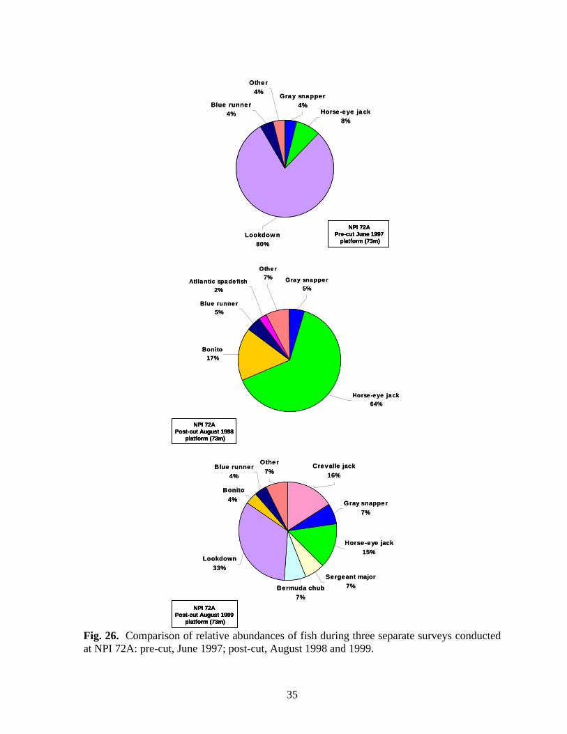
NPI 72APre-cut June 1997
platform (73m)
NPI 72APost-cut August 1998
platform (73m)
Gray snapper5%
Other7%Atllantic spade fish
2%
Blue runner5%
Horse-eye jack64%
Bonito17%
NPI 72APost-cut August 1999
platform (73m)
Lookdow n80%
Horse-eye jack8%
Gray snapper4%
Other4%
Blue runner4%
Bonito4%
Lookdown33%
Other7%
Crevalle jack16%
Gray snapper7%
Horse-eye jack15%
Sergeant major7%Bermuda chub
7%
Blue runner4%
NPI 72APre-cut June 1997
platform (73m)
NPI 72APre-cut June 1997
platform (73m)
NPI 72APost-cut August 1998
platform (73m)
NPI 72APost-cut August 1998
platform (73m)
Gray snapper5%
Other7%Atllantic spade fish
2%
Blue runner5%
Horse-eye jack64%
Bonito17%
NPI 72APost-cut August 1999
platform (73m)
NPI 72APost-cut August 1999
platform (73m)
Lookdow n80%
Horse-eye jack8%
Gray snapper4%
Other4%
Blue runner4%
Bonito4%
Lookdown33%
Other7%
Crevalle jack16%
Gray snapper7%
Horse-eye jack15%
Sergeant major7%Bermuda chub
7%
Blue runner4%
Fig. 26. Comparison of relative abundances of fish during three separate surveys conducted at NPI 72A: pre-cut, June 1997; post-cut, August 1998 and 1999.
35
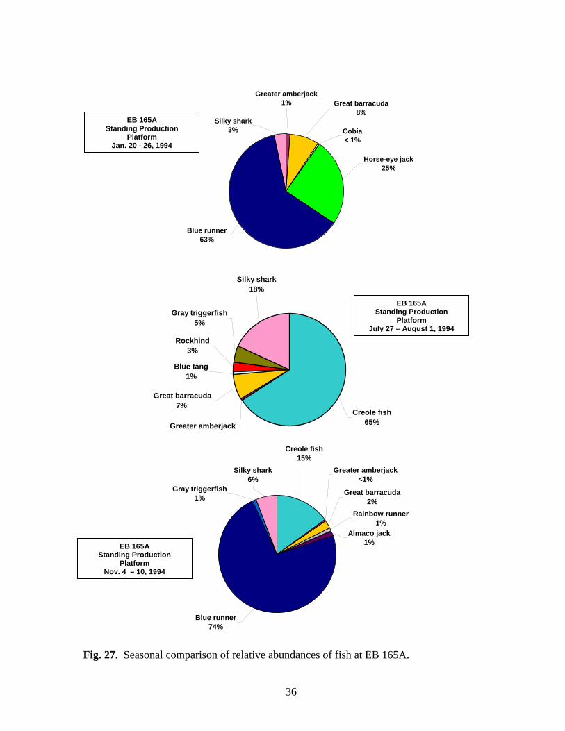
Great barracuda8%
Greater amberjack1%
Cobia< 1%
Silky shark3%
Blue runner63%
Horse-eye jack25%
EB 165A Standing Production
Platform Jan. 20 - 26, 1994
Creole fish65%
Silky shark18%
Gray triggerfish5%
Rockhind3%
Great barracuda7%
Greater amberjack
Blue tang1%
EB 165A Standing Production
Platform July 27 – August 1, 1994
Blue runner74%
Rainbow runner1%
Almaco jack1%
Silky shark6%
Creole fish15%
Great barracuda2%
Greater amberjack <1%
Gray triggerfish1%
EB 165A Standing Production
Platform Nov. 4 – 10, 1994
Fig. 27. Seasonal comparison of relative abundances of fish at EB 165A.
36
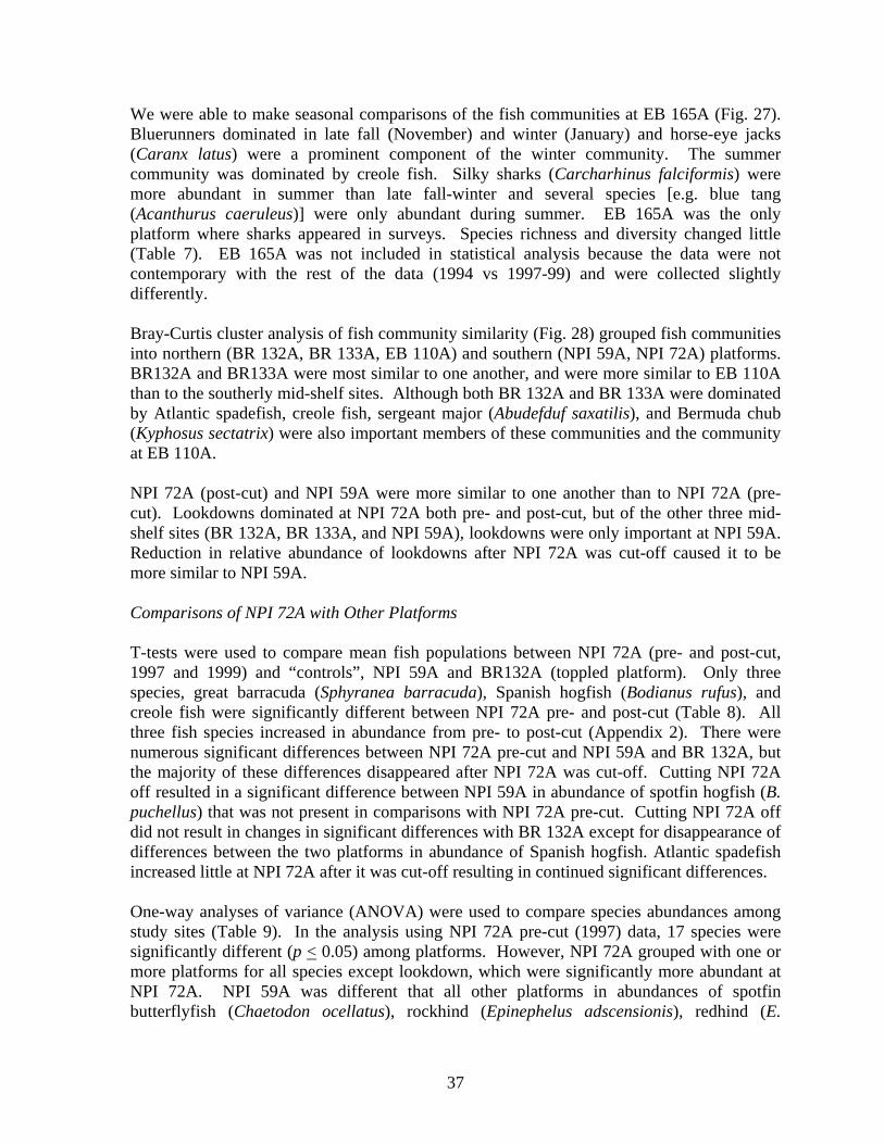
We were able to make seasonal comparisons of the fish communities at EB 165A (Fig. 27). Bluerunners dominated in late fall (November) and winter (January) and horse-eye jacks (Caranx latus) were a prominent component of the winter community. The summer community was dominated by creole fish. Silky sharks (Carcharhinus falciformis) were more abundant in summer than late fall-winter and several species [e.g. blue tang (Acanthurus caeruleus)] were only abundant during summer. EB 165A was the only platform where sharks appeared in surveys. Species richness and diversity changed little (Table 7). EB 165A was not included in statistical analysis because the data were not contemporary with the rest of the data (1994 vs 1997-99) and were collected slightly differently. Bray-Curtis cluster analysis of fish community similarity (Fig. 28) grouped fish communities into northern (BR 132A, BR 133A, EB 110A) and southern (NPI 59A, NPI 72A) platforms. BR132A and BR133A were most similar to one another, and were more similar to EB 110A than to the southerly mid-shelf sites. Although both BR 132A and BR 133A were dominated by Atlantic spadefish, creole fish, sergeant major (Abudefduf saxatilis), and Bermuda chub (Kyphosus sectatrix) were also important members of these communities and the community at EB 110A. NPI 72A (post-cut) and NPI 59A were more similar to one another than to NPI 72A (pre-cut). Lookdowns dominated at NPI 72A both pre- and post-cut, but of the other three mid-shelf sites (BR 132A, BR 133A, and NPI 59A), lookdowns were only important at NPI 59A. Reduction in relative abundance of lookdowns after NPI 72A was cut-off caused it to be more similar to NPI 59A. Comparisons of NPI 72A with Other Platforms
T-tests were used to compare mean fish populations between NPI 72A (pre- and post-cut, 1997 and 1999) and “controls”, NPI 59A and BR132A (toppled platform). Only three species, great barracuda (Sphyranea barracuda), Spanish hogfish (Bodianus rufus), and creole fish were significantly different between NPI 72A pre- and post-cut (Table 8). All three fish species increased in abundance from pre- to post-cut (Appendix 2). There were numerous significant differences between NPI 72A pre-cut and NPI 59A and BR 132A, but the majority of these differences disappeared after NPI 72A was cut-off. Cutting NPI 72A off resulted in a significant difference between NPI 59A in abundance of spotfin hogfish (B. puchellus) that was not present in comparisons with NPI 72A pre-cut. Cutting NPI 72A off did not result in changes in significant differences with BR 132A except for disappearance of differences between the two platforms in abundance of Spanish hogfish. Atlantic spadefish increased little at NPI 72A after it was cut-off resulting in continued significant differences. One-way analyses of variance (ANOVA) were used to compare species abundances among study sites (Table 9). In the analysis using NPI 72A pre-cut (1997) data, 17 species were significantly different (p < 0.05) among platforms. However, NPI 72A grouped with one or more platforms for all species except lookdown, which were significantly more abundant at NPI 72A. NPI 59A was different that all other platforms in abundances of spotfin butterflyfish (Chaetodon ocellatus), rockhind (Epinephelus adscensionis), redhind (E.
37
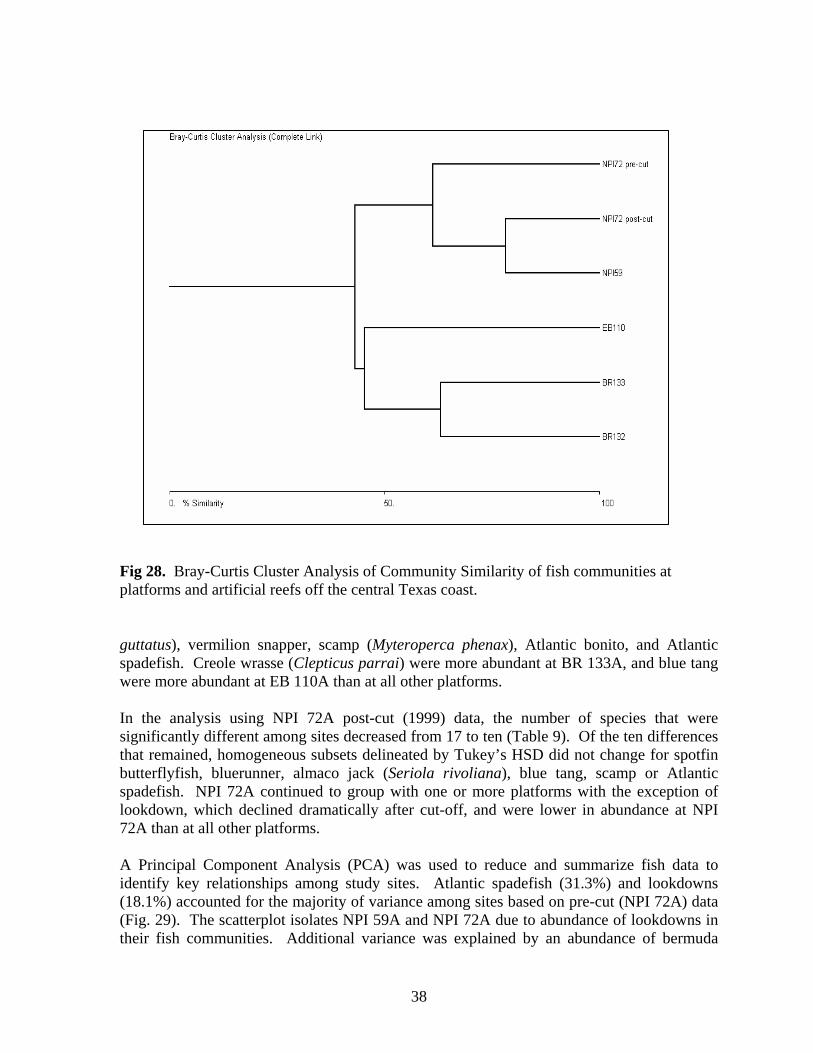
Fig 28. Bray-Curtis Cluster Analysis of Community Similarity of fish communities at platforms and artificial reefs off the central Texas coast. guttatus), vermilion snapper, scamp (Myteroperca phenax), Atlantic bonito, and Atlantic spadefish. Creole wrasse (Clepticus parrai) were more abundant at BR 133A, and blue tang were more abundant at EB 110A than at all other platforms. In the analysis using NPI 72A post-cut (1999) data, the number of species that were significantly different among sites decreased from 17 to ten (Table 9). Of the ten differences that remained, homogeneous subsets delineated by Tukey’s HSD did not change for spotfin butterflyfish, bluerunner, almaco jack (Seriola rivoliana), blue tang, scamp or Atlantic spadefish. NPI 72A continued to group with one or more platforms with the exception of lookdown, which declined dramatically after cut-off, and were lower in abundance at NPI 72A than at all other platforms. A Principal Component Analysis (PCA) was used to reduce and summarize fish data to identify key relationships among study sites. Atlantic spadefish (31.3%) and lookdowns (18.1%) accounted for the majority of variance among sites based on pre-cut (NPI 72A) data (Fig. 29). The scatterplot isolates NPI 59A and NPI 72A due to abundance of lookdowns in their fish communities. Additional variance was explained by an abundance of bermuda
38
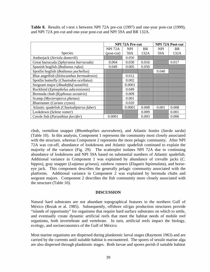
Table 8. Results of t-test s between NPI 72A pre-cut (1997) and one-year post-cut (1999), and NPI 72A pre-cut and one-year post-cut and NPI 59A and BR 132A.
NPI 72A Pre-cut NPI 72A Post-cut
Species NPI 72A (post-cut)
NPI 59A
BR 132A
NPI 59A
BR 132A
Amberjack (Seriola dumerili) 0.050 Great barracuda (Sphyranea barracuda) 0.004 0.030 0.016 0.017 Spanish hogfish (Bodianus rufus) 0.049 0.005 0.050 Spotfin hogfish (Bodianus puchellus) 0.040 Blue angelfish (Holocanthus bermudensis) 0.012 Spotfin butterfly (Chaetodon ocellatus) 0.002 Sergeant major (Abudefduf saxatilis) 0.0001 Rockhind (Epinephelus adscensionis) 0.049 Bermuda chub (Kyphosus sectatrix) 0.009 Scamp (Mycteroperca phenax) 0.001 Bluerunner (Caranx crysos) 0.020 Atlantic spadefish (Chaetodipterus faber) 0.0001 0.008 0.001 0.008 Lookdown (Selene vomer) 0.009 0.001 Creole fish (Paranthias furcifer) 0.0001 0.003 0.006
chub, vermilion snapper (Rhomboplites aurorubens), and Atlantic bonito (Sarda sarda) (Table 10). In this analysis, Component 1 represents the community most closely associated with the structure, whereas Component 2 represents the more pelagic community. After NPI 72A was cut-off, abundance of lookdowns and Atlantic spadefish continued to explain the majority of the variance (Fig. 29). The scatterplot isolates NPI 72A due to continuing abundance of lookdowns and NPI 59A based on substantial numbers of Atlantic spadefish. Additional variance in Component 1 was explained by abundance of crevalle jacks (C. hippos), gray snapper (Lutjanus griseus), rainbow runners (Elagatis bipinnulata), and horse-eye jack. This component describes the generally pelagic community associated with the platforms. Additional variance in Component 2 was explained by bermuda chubs and sergeant majors. Component 2 describes the fish community more closely associated with the structure (Table 10).
DISCUSSION Natural hard substrates are not abundant topographical features in the northern Gulf of México (Rezak et al. 1985). Subsequently, offshore oil/gas production structures provide “islands of opportunity” for organisms that require hard surface substrates on which to settle, and eventually create dynamic artificial reefs that meet the habitat needs of mobile reef organisms, both invertebrate and vertebrate. In turn, artificial reefs impact the biology, ecology, and socioeconomics of the Gulf of México. Most marine organisms are dispersed during planktonic larval stages (Raymont 1963) and are carried by the currents until suitable habitat is encountered. The spores of sessile marine alga are also dispersed through planktonic stages. Both larvae and spores perish if suitable habitat
39
Table 9. Results of one-way ANOVA’s (df 4, 15) and Tukey’s HSD comparing fish abundances among platforms. Analyses were performed separately on data from NPI 72A pre-cut (1997) and one-year post-cut (1999). EB 165A data is not included because it was not contemporary with the rest of the surveys. Sites are arranged from higher to lower abundance in homogenous subsets. 1 = BR 132A; 2 = BR 133A; 3 = NP I59A; 4 = NP-I72A; 5 = EB 110A
p Homogenous Subsets Species Pre-cut Post-cut Pre-cut Pos-tcut
Creole fish (Paranthias furcifer) 0.0001 0.003 1 5 2 3 4
1 5 2 3 4
Creole wrasse (Clepticus parrai) 0.0001 0.0001 2 1 3 4 5 2 5 4 3 1
Great Barracuda (Sphyranea barracuda) 0.008 0.029 1 3 2 5 4
1 2 3 4 5
Spanish hogfish (Bodianus puchellus) 0.047 1 3 2 4 5
Spotfin butterflyfish (Chaetodon ocellatus)
0.001 0.018 3 1 2 4 5 3 1 2 4 5
Rainbow runner (Elagatis bipinnulata) 0.017 1 4 5 3 2
Bluerunner (Caranx crysos) 0.005 0.017 3 5 4 1 2
1 2 4 5 3
Almaco jack (Seriola rivoliana) 0.046 0.045 1 4 2 3 5
1 4 2 3 5
Sergeant major (Abudefduf saxatilis) 0.007 3 2 1 4 5
Blue tang (Acanthurus coeruleus)
0.002 0.006 5 1 2 3 4 5 1 2 3 4
Rockhind (Epinephelus adscensionis) 0.008 3 1 2 4 5
Redhind (Epinephelus guttatus) 0.040 3 1 2 4 5
Vermilion snapper (Rhomboplites aurorubens)
0.037 3 1 2 4 5
Scamp (Myteroperca phenax)
0.0001 0.001 3 1 2 4 5 3 1 2 4 5
Lookdown (Selene vomer)
0.001 0.0001 4 1 2 3 5 3 1 2 5 4
Atlantic bonito (Sarda sarda)
0.037 3 1 2 4 5
Atlantic spadefish (Chaetodipterus faber)
0.0001 0.0001 1 2 3 4 5 1 2 3 4 5
40
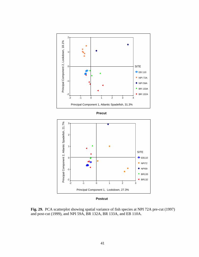
Principal Component 1, Atlantic Spadefish, 31.3%
43210-1-2
Prin
cipa
l Com
pone
nt 2
, Loo
kdow
n, 1
8.1%
2
1
0
-1
-2
SITE
EB 110
NPI 72A
NPI 59A
BR 133A
BR 132A
Precut
Principal Component 1, Lookdown, 27.3%
3210-1-2Prin
cipa
l Com
pone
nt 2
, Atla
ntic
Spa
defis
h, 2
1.7% 3
2
1
0
-1
-2
SITE
EB110
NPI72
NPI59
BR133
BR132
Postcut
Fig. 29. PCA scatterplot showing spatial variance of fish species at NPI 72A pre-cut (1997) and post-cut (1999), and NPI 59A, BR 132A, BR 133A, and EB 110A.
41
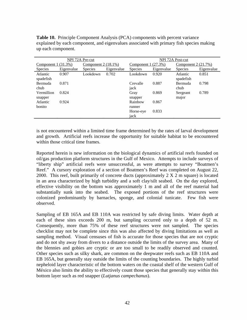
Table 10. Principle Component Analysis (PCA) components with percent variance explained by each component, and eigenvalues associated with primary fish species making up each component.
NPI 72A Pre-cut NPI 72A Post-cut
Component 1 (31.3%) Component 2 (18.1%) Component 1 (27.3%) Component 2 (21.7%)
Species Eigenvalue Species Eigenvalue Species Eigenvalue Species Eigenvalue Atlantic spadefish
0.907 Lookdown 0.702 Lookdown 0.920 Atlantic spadefish
0.851
Bermuda chub
0.871 Crevalle jack
0.887 Bermuda chub
0.798
Vermillion snapper
0.824 Gray snapper
0.869 Sergeant major
0.789
Atlantic bonito
0.924 Rainbow runner
0.867
Horse-eye jack
0.833
is not encountered within a limited time frame determined by the rates of larval development and growth. Artificial reefs increase the opportunity for suitable habitat to be encountered within those critical time frames.
Reported herein is new information on the biological dynamics of artificial reefs founded on oil/gas production platform structures in the Gulf of Mexico. Attempts to include surveys of “liberty ship” artificial reefs were unsuccessful, as were attempts to survey “Boatmen’s Reef.” A cursory exploration of a section of Boatmen’s Reef was completed on August 22, 2000. This reef, built primarily of concrete ducts (approximately 2 X 2 m square) is located in an area characterized by high turbidity and a soft clay/silt seabed. On the day explored, effective visibility on the bottom was approximately 1 m and all of the reef material had substantially sunk into the seabed. The exposed portions of the reef structures were colonized predominantly by barnacles, sponge, and colonial tunicate. Few fish were observed. Sampling of EB 165A and EB 110A was restricted by safe diving limits. Water depth at each of these sites exceeds 200 m, but sampling occurred only to a depth of 52 m. Consequently, more than 75% of these reef structures were not sampled. The species checklist may not be complete since this was also affected by diving limitations as well as sampling method. Visual censuses of fish is accurate for those species that are not cryptic and do not shy away from divers to a distance outside the limits of the survey area. Many of the blennies and gobies are cryptic or are too small to be readily observed and counted. Other species such as silky shark, are common on the deepwater reefs such as EB 110A and EB 165A, but generally stay outside the limits of the counting boundaries. The highly turbid nepheloid layer characteristic of the bottom waters on the coastal shelf of the western Gulf of México also limits the ability to effectively count those species that generally stay within this bottom layer such as red snapper (Lutjanus campechanus).
42
Biofouling Community
Many factors influence the characteristics of biofouling communities on platform structure artificial reefs (Fig. 2). Abiotic factors such as light penetration (Thorson 1964; Gunter and Geyer 1955), temperature, currents (Crisp 1974), depth and season (Odum, 1969), and biotic factors such as competition and predation (Connell, 1961; Paine, 1974; Webster, 1983) affect both abundance and distribution of sessile macroalgae and biofouling invertebrates. Generally, using the sessile fouling community to describe distinct biogenic zones, the results of this study are in agreement with Gallaway and Lewbell (1982) who described an east to west (i.e. shallow to deep water) change in community character. The nearshore to 30 m water depth was described as temperate “coastal.” The “offshore” zone, 30 to 60 m depth, was described as a mixture of the coastal and tropical “blue-water” zone beyond 60 m water depth. MU 746A, the nearest study site to shore in this study, was unique, and represented what we would have predicted for the Boatmen’s Reef and the Port Mansfield Liberty Ship reef. NPI 72A, BR 132A, and BR 133A constituted an offshore group, while EB 110A, EB 165A, and NPI 59A were similar enough in species composition to fit the blue-water group. The one surprise in this grouping is the similarity of NPI 59A to EB 110A and EB 165A. Logically, we would have predicted NPI 59A to be most similar, if not identical, to NPI 72A.
Each reef supports a fouling community of hundreds to thousands of kilograms of biomass. The sessile community, once established, is composed of permanent residents that, for the most part, release planktonic larvae, an export of energy and biomass. The fouling community contributes a steady rain of organic matter to the seabed, establishing greater habitat diversity and energy transport. Rooker et al. (1997) and Beaver (2000) established the importance of the fouling community to the fish community, both for shelter and food. Rooker et al. described diurnal cover seeking behavior of smaller reef fish and Beaver described seasonal shifts in food sources from the planktonic to the cryptic inhabitants of the fouling community. Existing across diverse water masses (i.e. temperate coastal, offshore, and tropical blue-water) within relatively short distance scales (i.e. ~ 145 km from coastal to blue-water environments), platform reefs provide the mechanism to support range extensions of marine organisms, effectively increasing local biodiversity. Rugosity, a linear measure of habitat surface complexity and indirect indication of microhabitat diversity, has been implicated in both the refuge needs of some fish species (Rooker et al. 1997) and the food needs of others (Beaver et al. 1997; Beaver 2000). Light intensity, food availability, mechanical energy, and species composition and morphology influence rugosity. In the upper zones, light increases plankton concentrations that can be exploited by filter-feeding, sessile invertebrates and provides more energy for photosynthesis within the sessile algal biomass. Mechanical energy (waves and currents) restricts the upper high-energy zone to those organisms and algae that have the morphological strength to withstand constant buffeting such as barnacles, tree oysters (Isognomon spp.), and some filamentous green algae. Based on our data and observations, increased rugosity creates more refuges and feeding opportunities for diurnally cryptic invertebrates and fish, juvenile reef fish, and nocturnal shelter-seeking fish. This increases biomass and biodiversity of the reef habitat both locally and regionally.
43
Observations suggest that the ubiquitous nepheloid layer of the northern Gulf of México impacts both the development and composition of the sessile invertebrate and fish communities. Biodiversity, microhabitat diversity, rugosity, and biomass appear to be negatively impacted by high turbidity. Blanketing the seabed (Shideler 1981), the nepheloid layer varies in thickness and concentration. It becomes more prevalent in nearshore, coastal waters, and due to decreasing water depths and incorporates and impacts a greater percentage of the vertical water column and reef structure. In low currents and water turbulence, sediments of the nepheloid layer settle on to exposed reef surfaces, smothering sessile plants and animals (Dokken et al. 1993b). On a hard substrate reef, many species settle within specific habitat zones defined by depth, while others are adapted to a broad range of depths (Dokken et al. 1993a, 1995; Dokken 1996; Adams 1995; Rooker et al. 1997; Riggs et al. 1998a, b). Vertical biogenic zones become more defined and lengthen as systems move into deeper, clearer water. Encrusting organisms become more morphologically varied. Species normally restricted to shallower biogenic zones (Megabalanus antillensis, Enteromorpha, Isognomon bicolor, and Ophiactis savignyi), begin to appear at deeper depths. Concurrently, species typically found in deeper zones coverage (i.e., Spondylus americanus, Helisarca sp., and Sertularia turbinata) expand their range upward into shallower depths with increased numbers and coverage. Fish Community Analysis of fish data grouped BR 132A, BR 133A, and EB 110A as a distinct grouping and NPI 59A and NPI 72A as a second distinct group. EB 165A was not included in the comparative analysis since it was collected before the rest of the data (1994) and not all fish were included in counts (e.g., sergeant major), but in general appeared similar to EB 110A. Fish data for MU 746A were not collected due to underwater visibility of less than 2 m during the sampling trip. Based on past observations at other coastal reefs, it is likely that MU 746A would have constituted a third distinct assemblage of fish just as the fouling community was distinct. These grouping also most strongly reflect an east to west (i.e., shallow to deep-water) transition of community character. Graphic representation of variations in the character of the fish communities at NPI 72A (Fig. 26) and EB 165A (Fig. 27) across multiple sampling periods clearly describe the dynamic nature of the fish communities. For the most part, carangids (Family Carangidae) were the primary agents of variation. This is not surprising since carangids are pelagic, very mobile, and maintain large school formations. Large schools of carangids moving around the Gulf encounter platform reefs by chance, and may take up short or long-term residence. Resident times are not known, but they probably fluctuate with season, food availability, as well as in response to other unknown parameters. Fish communities were dominated by planktivorous omnivores (e.g. Atlantic spadefish, lookdown, bluerunner, creole fish, Bermuda chub, and creole wrasse). This is consistent with reports by Stanley and Wilson (2000) for acoustical surveys of fishes on platform reefs off the Louisiana coast, and is consistent with natural reef communities (Hobson 1974, 1991; Sale 1991). Beaver (2000) described the role of these planktivores in transferring biological
44
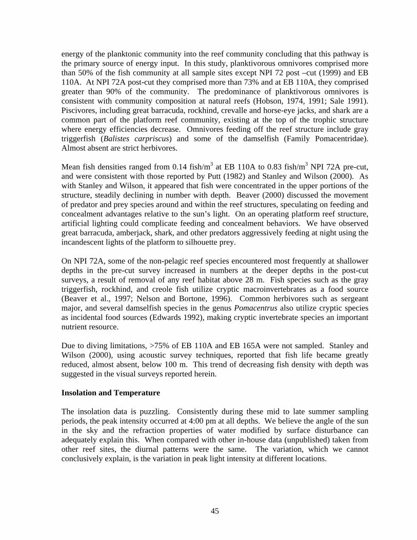
energy of the planktonic community into the reef community concluding that this pathway is the primary source of energy input. In this study, planktivorous omnivores comprised more than 50% of the fish community at all sample sites except NPI 72 post –cut (1999) and EB 110A. At NPI 72A post-cut they comprised more than 73% and at EB 110A, they comprised greater than 90% of the community. The predominance of planktivorous omnivores is consistent with community composition at natural reefs (Hobson, 1974, 1991; Sale 1991). Piscivores, including great barracuda, rockhind, crevalle and horse-eye jacks, and shark are a common part of the platform reef community, existing at the top of the trophic structure where energy efficiencies decrease. Omnivores feeding off the reef structure include gray triggerfish (Balistes carpriscus) and some of the damselfish (Family Pomacentridae). Almost absent are strict herbivores. Mean fish densities ranged from 0.14 fish/m3 at EB 110A to 0.83 fish/m3 NPI 72A pre-cut, and were consistent with those reported by Putt (1982) and Stanley and Wilson (2000). As with Stanley and Wilson, it appeared that fish were concentrated in the upper portions of the structure, steadily declining in number with depth. Beaver (2000) discussed the movement of predator and prey species around and within the reef structures, speculating on feeding and concealment advantages relative to the sun’s light. On an operating platform reef structure, artificial lighting could complicate feeding and concealment behaviors. We have observed great barracuda, amberjack, shark, and other predators aggressively feeding at night using the incandescent lights of the platform to silhouette prey. On NPI 72A, some of the non-pelagic reef species encountered most frequently at shallower depths in the pre-cut survey increased in numbers at the deeper depths in the post-cut surveys, a result of removal of any reef habitat above 28 m. Fish species such as the gray triggerfish, rockhind, and creole fish utilize cryptic macroinvertebrates as a food source (Beaver et al., 1997; Nelson and Bortone, 1996). Common herbivores such as sergeant major, and several damselfish species in the genus Pomacentrus also utilize cryptic species as incidental food sources (Edwards 1992), making cryptic invertebrate species an important nutrient resource. Due to diving limitations, >75% of EB 110A and EB 165A were not sampled. Stanley and Wilson (2000), using acoustic survey techniques, reported that fish life became greatly reduced, almost absent, below 100 m. This trend of decreasing fish density with depth was suggested in the visual surveys reported herein. Insolation and Temperature The insolation data is puzzling. Consistently during these mid to late summer sampling periods, the peak intensity occurred at 4:00 pm at all depths. We believe the angle of the sun in the sky and the refraction properties of water modified by surface disturbance can adequately explain this. When compared with other in-house data (unpublished) taken from other reef sites, the diurnal patterns were the same. The variation, which we cannot conclusively explain, is the variation in peak light intensity at different locations.
45
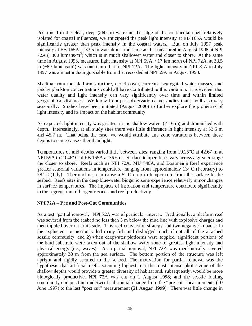
Positioned in the clear, deep (260 m) water on the edge of the continental shelf relatively isolated for coastal influences, we anticipated the peak light intensity at EB 165A would be significantly greater than peak intensity in the coastal waters. But, on July 1997 peak intensity at EB 165A at 33.5 m was almost the same as that measured in August 1998 at NPI 72A (~800 lumens/m2) which is in much shallower water and closer to shore. At the same time in August 1998, measured light intensity at NPI 59A, ~17 km north of NPI 72A, at 33.5 m (~80 lumens/m2) was one-tenth that of NPI 72A. The light intensity at NPI 72A in July 1997 was almost indistinguishable from that recorded at NPI 59A in August 1998.
Shading from the platform structure, cloud cover, currents, segregated water masses, and patchy plankton concentrations could all have contributed to this variation. It is evident that water quality and light intensity can vary significantly over time and within limited geographical distances. We know from past observations and studies that it will also vary seasonally. Studies have been initiated (August 2000) to further explore the properties of light intensity and its impact on the habitat community. As expected, light intensity was greatest in the shallow waters (< 16 m) and diminished with depth. Interestingly, at all study sites there was little difference in light intensity at 33.5 m and 45.7 m. That being the case, we would attribute any zone variations between these depths to some cause other than light. Temperatures of mid depths varied little between sites, ranging from 19.25oC at 42.67 m at NPI 59A to 20.46º C at EB 165A at 36.6 m. Surface temperatures vary across a greater range the closer to shore. Reefs such as NPI 72A, MU 746A, and Boatmen’s Reef experience greater seasonal variations in temperature, ranging from approximately 13º C (February) to 28º C (July). Thermoclines can cause a 5º C drop in temperature from the surface to the seabed. Reefs sites in the deep blue-water biogenic zone experience relatively minor changes in surface temperatures. The impacts of insolation and temperature contribute significantly to the segregation of biogenic zones and reef productivity. NPI 72A – Pre and Post-Cut Communities As a test “partial removal,” NPI 72A was of particular interest. Traditionally, a platform reef was severed from the seabed no less than 5 m below the mud line with explosive charges and then toppled over on to its side. This reef conversion strategy had two negative impacts: 1) the explosive concussion killed many fish and dislodged much if not all of the attached sessile community, and 2) when deepwater platforms were toppled, significant portions of the hard substrate were taken out of the shallow water zone of greatest light intensity and physical energy (i.e., waves). As a partial removal, NPI 72A was mechanically severed approximately 28 m from the sea surface. The bottom portion of the structure was left upright and rigidly secured to the seabed. The motivation for partial removal was the hypothesis that artificial reefs extending highest into the most intense photic zone of the shallow depths would provide a greater diversity of habitat and, subsequently, would be more biologically productive. NPI 72A was cut on 1 August 1998; and the sessile fouling community composition underwent substantial change from the “pre-cut” measurements (10 June 1997) to the last “post cut” measurement (21 August 1999). There was little change in
46
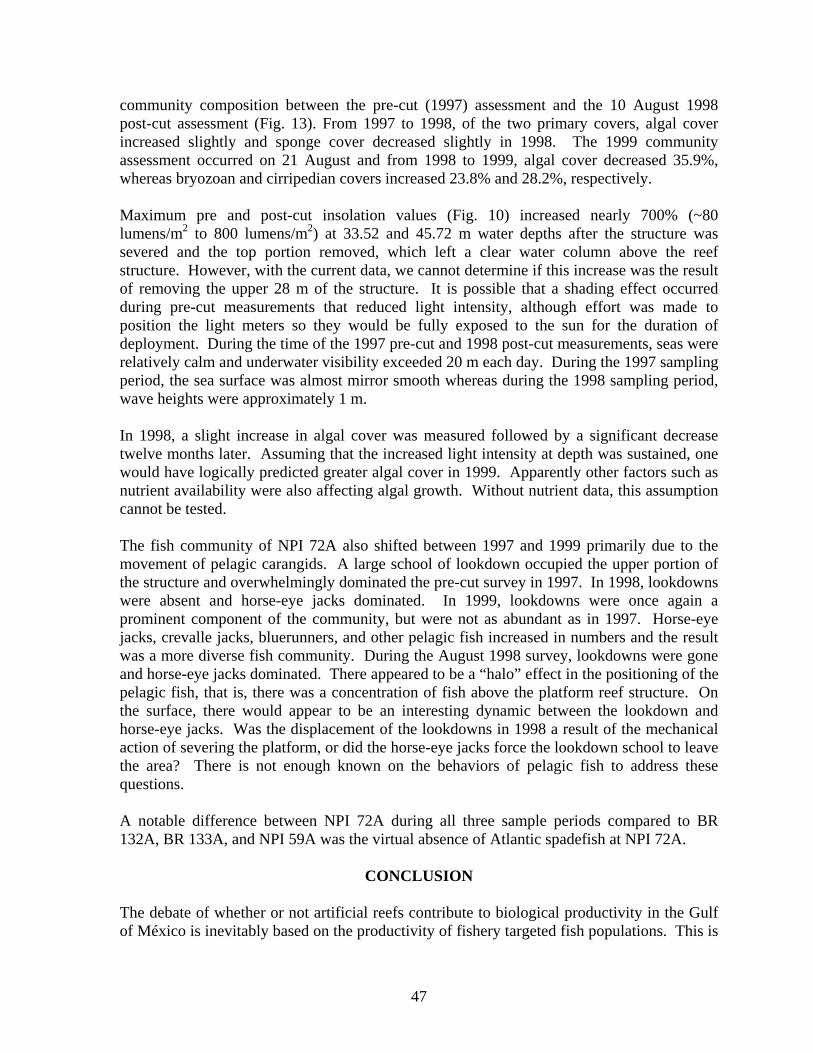
community composition between the pre-cut (1997) assessment and the 10 August 1998 post-cut assessment (Fig. 13). From 1997 to 1998, of the two primary covers, algal cover increased slightly and sponge cover decreased slightly in 1998. The 1999 community assessment occurred on 21 August and from 1998 to 1999, algal cover decreased 35.9%, whereas bryozoan and cirripedian covers increased 23.8% and 28.2%, respectively. Maximum pre and post-cut insolation values (Fig. 10) increased nearly 700% (~80 lumens/m2 to 800 lumens/m2) at 33.52 and 45.72 m water depths after the structure was severed and the top portion removed, which left a clear water column above the reef structure. However, with the current data, we cannot determine if this increase was the result of removing the upper 28 m of the structure. It is possible that a shading effect occurred during pre-cut measurements that reduced light intensity, although effort was made to position the light meters so they would be fully exposed to the sun for the duration of deployment. During the time of the 1997 pre-cut and 1998 post-cut measurements, seas were relatively calm and underwater visibility exceeded 20 m each day. During the 1997 sampling period, the sea surface was almost mirror smooth whereas during the 1998 sampling period, wave heights were approximately 1 m. In 1998, a slight increase in algal cover was measured followed by a significant decrease twelve months later. Assuming that the increased light intensity at depth was sustained, one would have logically predicted greater algal cover in 1999. Apparently other factors such as nutrient availability were also affecting algal growth. Without nutrient data, this assumption cannot be tested.
The fish community of NPI 72A also shifted between 1997 and 1999 primarily due to the movement of pelagic carangids. A large school of lookdown occupied the upper portion of the structure and overwhelmingly dominated the pre-cut survey in 1997. In 1998, lookdowns were absent and horse-eye jacks dominated. In 1999, lookdowns were once again a prominent component of the community, but were not as abundant as in 1997. Horse-eye jacks, crevalle jacks, bluerunners, and other pelagic fish increased in numbers and the result was a more diverse fish community. During the August 1998 survey, lookdowns were gone and horse-eye jacks dominated. There appeared to be a “halo” effect in the positioning of the pelagic fish, that is, there was a concentration of fish above the platform reef structure. On the surface, there would appear to be an interesting dynamic between the lookdown and horse-eye jacks. Was the displacement of the lookdowns in 1998 a result of the mechanical action of severing the platform, or did the horse-eye jacks force the lookdown school to leave the area? There is not enough known on the behaviors of pelagic fish to address these questions.
A notable difference between NPI 72A during all three sample periods compared to BR 132A, BR 133A, and NPI 59A was the virtual absence of Atlantic spadefish at NPI 72A.
CONCLUSION The debate of whether or not artificial reefs contribute to biological productivity in the Gulf of México is inevitably based on the productivity of fishery targeted fish populations. This is
47
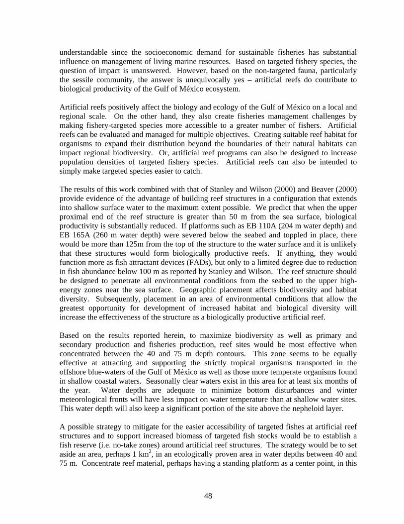
understandable since the socioeconomic demand for sustainable fisheries has substantial influence on management of living marine resources. Based on targeted fishery species, the question of impact is unanswered. However, based on the non-targeted fauna, particularly the sessile community, the answer is unequivocally yes – artificial reefs do contribute to biological productivity of the Gulf of México ecosystem. Artificial reefs positively affect the biology and ecology of the Gulf of México on a local and regional scale. On the other hand, they also create fisheries management challenges by making fishery-targeted species more accessible to a greater number of fishers. Artificial reefs can be evaluated and managed for multiple objectives. Creating suitable reef habitat for organisms to expand their distribution beyond the boundaries of their natural habitats can impact regional biodiversity. Or, artificial reef programs can also be designed to increase population densities of targeted fishery species. Artificial reefs can also be intended to simply make targeted species easier to catch. The results of this work combined with that of Stanley and Wilson (2000) and Beaver (2000) provide evidence of the advantage of building reef structures in a configuration that extends into shallow surface water to the maximum extent possible. We predict that when the upper proximal end of the reef structure is greater than 50 m from the sea surface, biological productivity is substantially reduced. If platforms such as EB 110A (204 m water depth) and EB 165A (260 m water depth) were severed below the seabed and toppled in place, there would be more than 125m from the top of the structure to the water surface and it is unlikely that these structures would form biologically productive reefs. If anything, they would function more as fish attractant devices (FADs), but only to a limited degree due to reduction in fish abundance below 100 m as reported by Stanley and Wilson. The reef structure should be designed to penetrate all environmental conditions from the seabed to the upper high-energy zones near the sea surface. Geographic placement affects biodiversity and habitat diversity. Subsequently, placement in an area of environmental conditions that allow the greatest opportunity for development of increased habitat and biological diversity will increase the effectiveness of the structure as a biologically productive artificial reef. Based on the results reported herein, to maximize biodiversity as well as primary and secondary production and fisheries production, reef sites would be most effective when concentrated between the 40 and 75 m depth contours. This zone seems to be equally effective at attracting and supporting the strictly tropical organisms transported in the offshore blue-waters of the Gulf of México as well as those more temperate organisms found in shallow coastal waters. Seasonally clear waters exist in this area for at least six months of the year. Water depths are adequate to minimize bottom disturbances and winter meteorological fronts will have less impact on water temperature than at shallow water sites. This water depth will also keep a significant portion of the site above the nepheloid layer. A possible strategy to mitigate for the easier accessibility of targeted fishes at artificial reef structures and to support increased biomass of targeted fish stocks would be to establish a fish reserve (i.e. no-take zones) around artificial reef structures. The strategy would be to set aside an area, perhaps 1 km2, in an ecologically proven area in water depths between 40 and 75 m. Concentrate reef material, perhaps having a standing platform as a center point, in this
48
area. Place the reef material in side by side, creating as much reef complexity and vertical relief as possible. Extend the reef structure to the shallowest depth allowable when considering shipping safety. There remains a great deal of research to be done to fully understand the impact of artificial reefs upon the ecology and productivity of the Gulf of México. With thoughtful consideration and planning based upon known facts of the dynamics of artificial reefs, they will contribute to meeting the ever-growing demand for marine resources and recreational opportunities.
49
LITERATURE CITED Adams, C. 1995. Species composition, abundance and depth zonation of sponges (phylum
Porifera) on an outer continental shelf gas production platform, northwestern Gulf of Mexico. M.S. thesis, Texas A&M University-Corpus Christi. Corpus Christi, Texas. 130 pp.
Beaver, C. R. 2000. Fishery productivity and trophodynamics of platform artificial reefs in
the Northwestern Gulf of Mexico (draft). Ph.D. dissertation, Texas A&M University. College Station, Texas. 93 pp.
Beaver, C. R., Q .R. Dokken and T. Riggs. 1997. Utilization of fouling community elements
by reef fishes at a platform artificial reef in the northwestern Gulf of Mexico, pp. 388-394. In Proceedings: Seventeenth Annual Gulf of Mexico Information Transfer Meeting. Minerals Management Service. New Orleans, Louisiana.
Bohnsack, J. A., A. M.Ecklund, and A. M. Szmant. 1997. Essay: Artificial reef research: is
there more than the attraction-production issue? Fisheries 22(4): 14-16. Bohnsack, J. A. and S. P. Bannerot. 1986. A stationary visual census technique for
quantitatively assessing community structure of coral reef fishes. NOAA Technical Report, NMFS 41. Silverspring, Maryland. 15 pp.
Carr, M. H. and M. A. Hixon. 1997. Artificial reefs: the importance of comparisons with
natural reefs. Fisheries 22(4): 28-33. Connell, J. H. 1961. The influence of interspecific competition and other factors on the distribution of the barnacle Chthamalus stellatus. Ecology 42: 710-723. Crisp, D. J. 1974. Factors influencing the settlement of marine invertebrate larvae, pp. 177-265. In P.T. Grant and A.M. Mackie (eds.), Chemoreception in Marine Organisms. Academic Press. New York, New York. Ditton, R., L. Finklestein, and J. Wilson. 1995. Use of offshore artificial reefs by Texas
charter fishing and diving boats. Texas A&M University Department of Wildlife and Fisheries Sciences Technical Report HD-604. College Station, Texas. 50 pp.
Dokken, Q. R. 1996. Platform reef ecological and biological productivity: fact or fiction?,
pp. 12-19. In Proceedings: Sixteenth Annual Gulf of Mexico Information Transfer Meeting. Minerals Management Service MMS96-0038. New Orleans, Louisiana.
Dokken, Q. R., C. Adams and B. Ponwith. 1993a. Preliminary survey of the artificial reef
complex in Mineral Lease Block High Island A298 and development of survey techniques for application to long-term monitoring. Texas A&M University-Corpus Christi, Center for Coastal Studies Technical Report No. TAMUCC-9302-CCS (#14). Corpus Christi, Texas. 44 pp.
50

Dokken, Q R., C. Beaver, S. Cox, C. Adams, J. Rooker, and J. Childs. 1995. Characterization of biofouling communities on oil and gas production platforms: impact on finfish assemblage, pp. 1-16. In Proceedings: Fifteenth Annual Gulf of Mexico Information Transfer Meeting. Minerals Management Service. New Orleans, Louisiana.
Dokken, Q., R. Lehman, J. Prouty, C. Adams, C. Beaver. 1993b. A preliminary survey of
Sebree Bank (Gulf of Mexico, Port Mansfield, Texas August 23-27, 1993). Texas A&M University-Corpus Christi, Center for Coastal Studies Technical Report No. TAMU-CC-9305-CCS. 13 pp.
Gallaway, B. J., M. F. Johnson, L. R. Martin, F. J. Margraf, G. S. Lewbel, R. L .Howard, and
G. S. Boland. 1981. The artificial reef studies, vol. 2. In C. A. Bedinger, Jr., and L. Z. Kirby, (eds.), Ecological Investigations of Petroleum Production Platforms in the Central Gulf of Mexico. Bureau of Land Management SWRI Project 01-5245. New Orleans, Louisiana.
Gallaway, B. J. and G. S. Lewbel. 1982. The ecology of petroleum platforms in the
northwestern Gulf of Mexico: a community profile. US Fish and Wildlife Service, Office of Biological Services FWS/OBS-82/27; Bureau of Land Management, Gulf of Mexico OCS Regional Office Open-File Report 82-03. 92 pp.
Grossman, G. D., G. P. Jones, and W. J. Seaman, Jr. 1997. Do artificial reefs increase regional fish production? A review of existing data. Fisheries 22(4): 17-23.
Gunter, G. and R .H. Geyer. 1955. Studies on fouling organisms of the northwest Gulf of
Mexico. Publications of the Institute of Marine Science, University of Texas 4(1): 37-68.
Hobson, E. S. 1974. Feeding patterns among tropical reef fishes. American Scientist 63:
389-392. Hobson, E. S. 1991. Trophic relationships of fishes specialized to feed on zooplankters
above coral reefs, pp. 69-95. In P. F. Sale (ed.), The Ecology of Fishes on Coral Reefs. Academic Press. New York, New York.
Lindberg, W. J. 1997. Essay: Can science resolve the attraction-production issue?
Fisheries 22(4): 10-13. Nelson, B. D. and S. A. Bortone. 1996. Feeding guilds among artificial-reef fishes in the
northern Gulf of Mexico. Gulf of Mexico Science 2: 66-80. Odum, E. P. 1969. The strategy of ecosystem development. Science 164: 262-270. Paine, R. T. 1974. Intertidal community structure: experimental studies on the relationship
between a dominant competitor and its principal predator. Oecologia 15: 93-120.
51
Putt, R. E., Jr. 1982. A quantitative study of fish populations associated with a platform within Buccaneer oil field, northwestern Gulf of Mexico. M.S. thesis, Texas A&M University. College Station, Texas. 116 pp.
Raymont, J. E .G. 1963. Plankton and Productivity in the Oceans. Pergamon Press. New
York, New York. 660 pp.
Reggio, V. C. Jr. 1989. Petroleum structures as artificial reefs: a compendium. Fourth international conference on artificial habitats for fisheries, rigs-to-reefs special session. OCS Study/MMS 89-0021. New Orleans, Louisiana. 176 pp.
Rezak, R., T. J. Bright and D. W. McGrail. 1985. Reefs and Banks of the Northwestern
Gulf of Mexico: Their Geological, Biological and Physical Dynamics. Wiley and Sons. New York, New York. 259 pp.
Riggs, T. E., C. R. Beaver and Q. R. Dokken. 1998a. Pre and Post –Cut Analysis of Fouling
Community on a Recently Installed Artificial Reef off South Padre Island, Texas, pp. 59-66. In Proceedings: Eighteenth Annual Gulf of Mexico Information Transfer Meeting. Minerals Management Service, OCS Study MMS 2000-030. New Orleans, Louisiana.
Riggs, T. E., C. R. Beaver, L. D.Vitale and Q. R. Dokken. 1998b. Preliminary ecological
survey Seagull Energy, Inc. platform NPI 72A off south Texas coast. Texas A&M University-Corpus Christi, Center for Coastal Studies Technical Report No. TAMU-CC-9803-CCS.
Rooker, J. R., Q. R. Dokken, C. V. Pattengill, and G. J. Holt. 1997. Fish assemblages on
artificial and natural reefs in the Flower Garden Banks National Marine Sanctuary. Coral Reefs 16: 83-92.
Sale, P. F. (ed.). 1991. The Ecology of Fishes on Coral Reefs. Academic Press. New York,
New York. 754 pp. Shideler, G. L. 1981. Development of the benthic nepheloid layer on the South Texas continental shelf, western Gulf of Mexico. Marine Geology 41: 37-61. Stanley, D. R. and C. A. Wilson. 2000. Seasonal and spatial variation in the biomass and
size frequency distribution of fish associated with oil and gas platforms in the northern Gulf of Mexico. Minerals Management Service, OCS Study 2000-005. New Orleans, Louisiana. 252 pp.
Thorson, G. 1964. Light as an ecological factor in the dispersal and settlement of larvae of
marine bottom invertebrates. Ophelia 1: 167- 208.
Webster, J. R. 1983. The role of macroinvertebrates in detritus dynamics of streams: a computer simulation. Ecological Monographs 53: 383-404.
52

APPENDICES
53

54

55

56

57

58

59

60

61

62

63

64

65
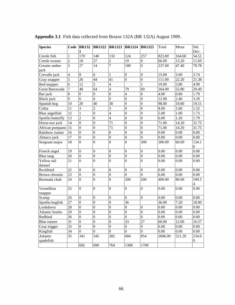
Appendix 3.1 Fish data collected from Brazos 132A (BR 132A) August 1999.
Species Code BR132
1 BR1322 BR1323 BR1324 BR1325 Total Mean Std.
Dev. Creole fish 1 170 140 132 124 257 823.00 164.60 54.51 Creole wrasse 2 18 27 2 19 0 66.00 13.20 11.69 Greater amber jack
3 27 14 7 189 0 237.00 47.40 79.78
Crevalle jack 4 8 6 1 0 0 15.00 3.00 3.74 Gray snapper 5 26 44 41 0 0 111.00 22.20 21.38 Red snapper 6 12 2 4 1 19.00 3.80 4.99 Great Barracuda 7 48 64 4 79 69 264.00 52.80 29.49 Bar jack 8 0 0 0 4 0 4.00 0.80 1.79 Black jack 9 6 6 0 0 0 12.00 2.40 3.29 Spanish hog 10 20 40 38 0 0 98.00 19.60 19.51 Cobia 11 3 2 3 0 0 8.00 1.60 1.52 Blue angelfish 12 1 0 4 0 0 5.00 1.00 1.73 Spotfin butterfly 13 2 0 4 0 0 6.00 1.20 1.79 Horse-eye jack 14 0 0 71 0 0 71.00 14.20 31.75 African pompano 15 0 0 71 0 0 71.00 14.20 31.75 Rainbow runner 16 0 0 0 0 0 0.00 0.00 0.00 Almaco jack 17 0 0 0 0 0 0.00 0.00 0.00 Sergeant major 18 0 0 0 0 300 300.00 60.00 134.1
6 French angel 19 0 0 0 0 0 0.00 0.00 0.00 Blue tang 20 0 0 0 0 0 0.00 0.00 0.00 Yellow tail damsel
21 0 0 0 0 0 0.00 0.00 0.00
Rockhind 22 0 0 0 0 0 0.00 0.00 0.00 Brown chromis 23 0 0 0 0 0 0.00 0.00 0.00 Bermuda chub 24 0 0 0 200 200 400.00 80.00 109.5
4 Vermillion snapper
25 0 0 0 0 0 0.00 0.00 0.00
Scamp 26 0 0 0 0 0 0.00 0.00 0.00 Spotfin hogfish 27 0 0 0 36 36.00 7.20 18.00 Lookdown 28 0 0 0 0 0 0.00 0.00 0.00 Atlantic bonito 29 0 0 0 0 0 0.00 0.00 0.00 Redhind 30 0 0 0 0 0 0.00 0.00 0.00 Blue runner 31 0 0 0 33 27 60.00 12.00 16.57 Gray trigger 33 0 0 0 0 0 0.00 0.00 0.00 Kingfish 34 0 0 0 0 0 0.00 0.00 0.00 Atlantic spadefish
35 341 345 382 684 854 2606.00 521.20 234.60
682 690 764 1368 1708
66
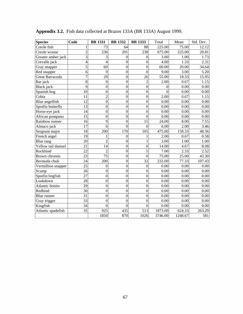
Appendix 3.2. Fish data collected at Brazos 133A (BR 133A) August 1999. Species Code BR 1331 BR 1332 BR 1333 Total Mean Std. Dev. Creole fish 1 73 64 88 225.00 75.00 12.12Creole wrasse 2 236 201 238 675.00 225.00 20.81Greater amber jack 3 3 0 0 3.00 1.00 1.73Crevalle jack 4 4 0 0 4.00 1.33 2.31Gray snapper 5 60 0 0 60.00 20.00 34.64Red snapper 6 9 0 0 9.00 3.00 5.20Great Barracuda 7 29 0 26 55.00 18.33 15.95Bar jack 8 0 0 2 2.00 0.67 1.15Black jack 9 0 0 0 0 0.00 0.00Spanish hog 10 0 0 0 0 0.00 0.00Cobia 11 2 0 0 2.00 0.67 1.15Blue angelfish 12 0 0 0 0.00 0.00 0.00Spotfin butterfly 13 0 0 0 0.00 0.00 0.00Horse-eye jack 14 0 0 0 0.00 0.00 0.00African pompano 15 0 0 0 0.00 0.00 0.00Rainbow runner 16 9 0 15 24.00 8.00 7.55Almaco jack 17 6 0 0 6.00 2.00 3.46Sergeant major 18 200 170 105 475.00 158.33 48.56French angel 19 1 0 1 2.00 0.67 0.58Blue tang 20 2 0 1 3.00 1.00 1.00Yellow tail damsel 21 14 0 0 14.00 4.67 8.08Rockhind 22 2 0 5 7.00 2.33 2.52Brown chromis 23 75 0 0 75.00 25.00 43.30Bermuda chub 24 200 0 32 232.00 77.33 107.43Vermillion snapper 25 0 0 0 0.00 0.00 0.00Scamp 26 0 0 0 0.00 0.00 0.00Spotfin hogfish 27 0 0 0 0.00 0.00 0.00Lookdown 28 0 0 0 0.00 0.00 0.00Atlantic bonito 29 0 0 0 0.00 0.00 0.00Redhind 30 0 0 0 0.00 0.00 0.00Blue runner 31 0 0 0 0.00 0.00 0.00Gray trigger 33 0 0 0 0.00 0.00 0.00Kingfish 34 0 0 0 0.00 0.00 0.00Atlantic spadefish 35 925 435 513 1873.00 624.33 263.29
1850 870 1026 3746.00 1248.67 581
67
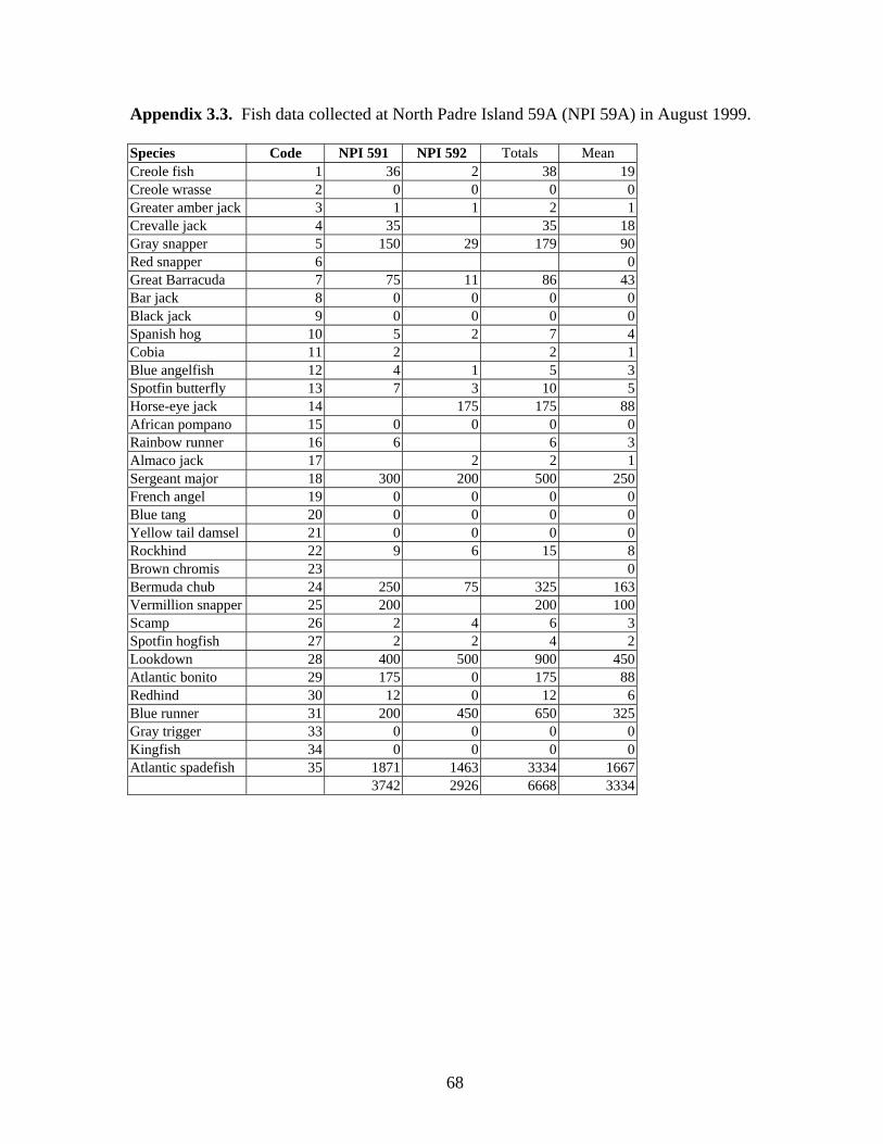
Appendix 3.3. Fish data collected at North Padre Island 59A (NPI 59A) in August 1999. Species Code NPI 591 NPI 592 Totals Mean Creole fish 1 36 2 38 19 Creole wrasse 2 0 0 0 0 Greater amber jack 3 1 1 2 1 Crevalle jack 4 35 35 18 Gray snapper 5 150 29 179 90 Red snapper 6 0 Great Barracuda 7 75 11 86 43 Bar jack 8 0 0 0 0 Black jack 9 0 0 0 0 Spanish hog 10 5 2 7 4 Cobia 11 2 2 1 Blue angelfish 12 4 1 5 3 Spotfin butterfly 13 7 3 10 5 Horse-eye jack 14 175 175 88 African pompano 15 0 0 0 0 Rainbow runner 16 6 6 3 Almaco jack 17 2 2 1 Sergeant major 18 300 200 500 250 French angel 19 0 0 0 0 Blue tang 20 0 0 0 0 Yellow tail damsel 21 0 0 0 0 Rockhind 22 9 6 15 8 Brown chromis 23 0 Bermuda chub 24 250 75 325 163 Vermillion snapper 25 200 200 100 Scamp 26 2 4 6 3 Spotfin hogfish 27 2 2 4 2 Lookdown 28 400 500 900 450 Atlantic bonito 29 175 0 175 88 Redhind 30 12 0 12 6 Blue runner 31 200 450 650 325 Gray trigger 33 0 0 0 0 Kingfish 34 0 0 0 0 Atlantic spadefish 35 1871 1463 3334 1667
3742 2926 6668 3334
68
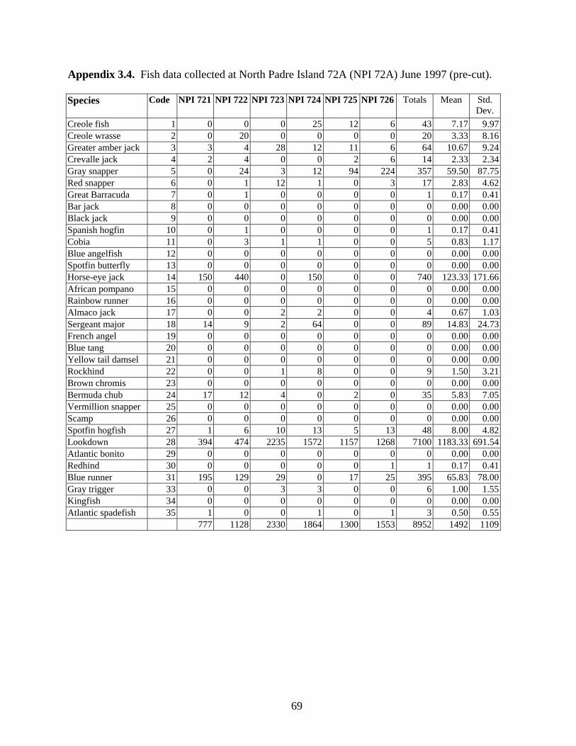
Appendix 3.4. Fish data collected at North Padre Island 72A (NPI 72A) June 1997 (pre-cut).
Species Code NPI 721 NPI 722 NPI 723 NPI 724 NPI 725 NPI 726 Totals Mean Std. Dev.
Creole fish 1 0 0 0 25 12 6 43 7.17 9.97Creole wrasse 2 0 20 0 0 0 0 20 3.33 8.16Greater amber jack 3 3 4 28 12 11 6 64 10.67 9.24Crevalle jack 4 2 4 0 0 2 6 14 2.33 2.34Gray snapper 5 0 24 3 12 94 224 357 59.50 87.75Red snapper 6 0 1 12 1 0 3 17 2.83 4.62Great Barracuda 7 0 1 0 0 0 0 1 0.17 0.41Bar jack 8 0 0 0 0 0 0 0 0.00 0.00Black jack 9 0 0 0 0 0 0 0 0.00 0.00Spanish hogfin 10 0 1 0 0 0 0 1 0.17 0.41Cobia 11 0 3 1 1 0 0 5 0.83 1.17Blue angelfish 12 0 0 0 0 0 0 0 0.00 0.00Spotfin butterfly 13 0 0 0 0 0 0 0 0.00 0.00Horse-eye jack 14 150 440 0 150 0 0 740 123.33 171.66African pompano 15 0 0 0 0 0 0 0 0.00 0.00Rainbow runner 16 0 0 0 0 0 0 0 0.00 0.00Almaco jack 17 0 0 2 2 0 0 4 0.67 1.03Sergeant major 18 14 9 2 64 0 0 89 14.83 24.73French angel 19 0 0 0 0 0 0 0 0.00 0.00Blue tang 20 0 0 0 0 0 0 0 0.00 0.00Yellow tail damsel 21 0 0 0 0 0 0 0 0.00 0.00Rockhind 22 0 0 1 8 0 0 9 1.50 3.21Brown chromis 23 0 0 0 0 0 0 0 0.00 0.00Bermuda chub 24 17 12 4 0 2 0 35 5.83 7.05Vermillion snapper 25 0 0 0 0 0 0 0 0.00 0.00Scamp 26 0 0 0 0 0 0 0 0.00 0.00Spotfin hogfish 27 1 6 10 13 5 13 48 8.00 4.82Lookdown 28 394 474 2235 1572 1157 1268 7100 1183.33 691.54Atlantic bonito 29 0 0 0 0 0 0 0 0.00 0.00Redhind 30 0 0 0 0 0 1 1 0.17 0.41Blue runner 31 195 129 29 0 17 25 395 65.83 78.00Gray trigger 33 0 0 3 3 0 0 6 1.00 1.55Kingfish 34 0 0 0 0 0 0 0 0.00 0.00Atlantic spadefish 35 1 0 0 1 0 1 3 0.50 0.55
777 1128 2330 1864 1300 1553 8952 1492 1109
69
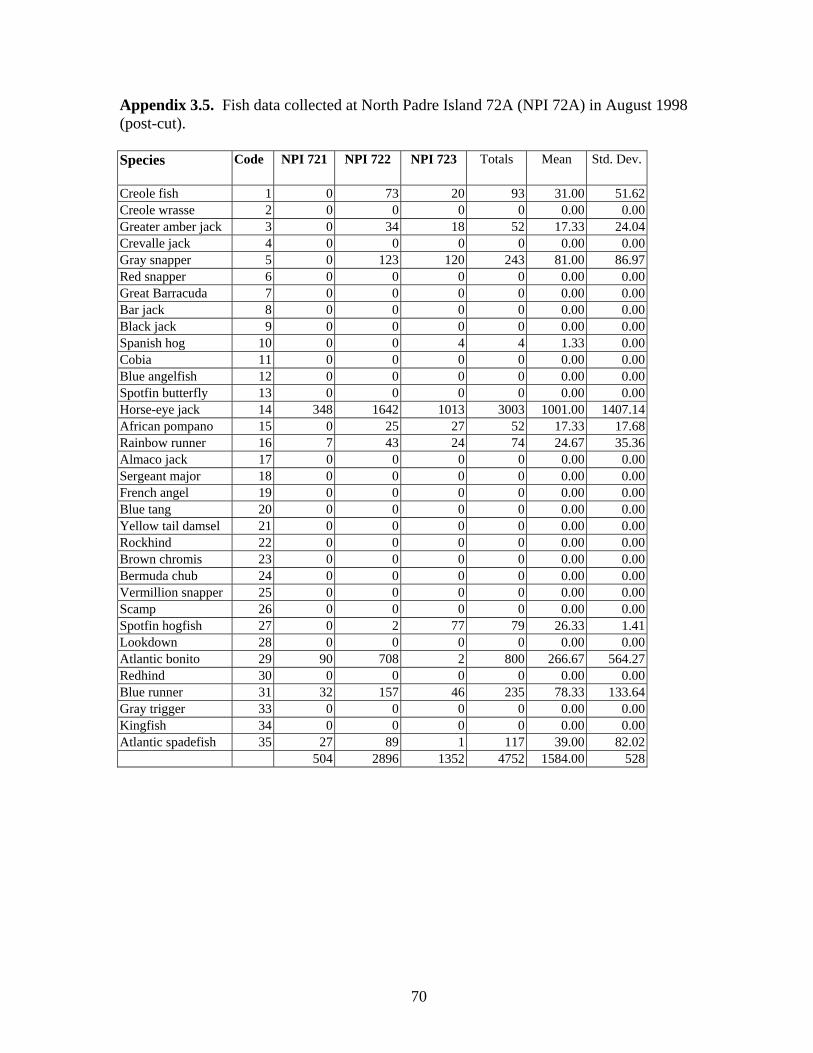
Appendix 3.5. Fish data collected at North Padre Island 72A (NPI 72A) in August 1998 (post-cut). Species Code NPI 721 NPI 722 NPI 723 Totals Mean Std. Dev.
Creole fish 1 0 73 20 93 31.00 51.62 Creole wrasse 2 0 0 0 0 0.00 0.00 Greater amber jack 3 0 34 18 52 17.33 24.04 Crevalle jack 4 0 0 0 0 0.00 0.00 Gray snapper 5 0 123 120 243 81.00 86.97 Red snapper 6 0 0 0 0 0.00 0.00 Great Barracuda 7 0 0 0 0 0.00 0.00 Bar jack 8 0 0 0 0 0.00 0.00 Black jack 9 0 0 0 0 0.00 0.00 Spanish hog 10 0 0 4 4 1.33 0.00 Cobia 11 0 0 0 0 0.00 0.00 Blue angelfish 12 0 0 0 0 0.00 0.00 Spotfin butterfly 13 0 0 0 0 0.00 0.00 Horse-eye jack 14 348 1642 1013 3003 1001.00 1407.14 African pompano 15 0 25 27 52 17.33 17.68 Rainbow runner 16 7 43 24 74 24.67 35.36 Almaco jack 17 0 0 0 0 0.00 0.00 Sergeant major 18 0 0 0 0 0.00 0.00 French angel 19 0 0 0 0 0.00 0.00 Blue tang 20 0 0 0 0 0.00 0.00 Yellow tail damsel 21 0 0 0 0 0.00 0.00 Rockhind 22 0 0 0 0 0.00 0.00 Brown chromis 23 0 0 0 0 0.00 0.00 Bermuda chub 24 0 0 0 0 0.00 0.00 Vermillion snapper 25 0 0 0 0 0.00 0.00 Scamp 26 0 0 0 0 0.00 0.00 Spotfin hogfish 27 0 2 77 79 26.33 1.41 Lookdown 28 0 0 0 0 0.00 0.00 Atlantic bonito 29 90 708 2 800 266.67 564.27 Redhind 30 0 0 0 0 0.00 0.00 Blue runner 31 32 157 46 235 78.33 133.64 Gray trigger 33 0 0 0 0 0.00 0.00 Kingfish 34 0 0 0 0 0.00 0.00 Atlantic spadefish 35 27 89 1 117 39.00 82.02
504 2896 1352 4752 1584.00 528
70
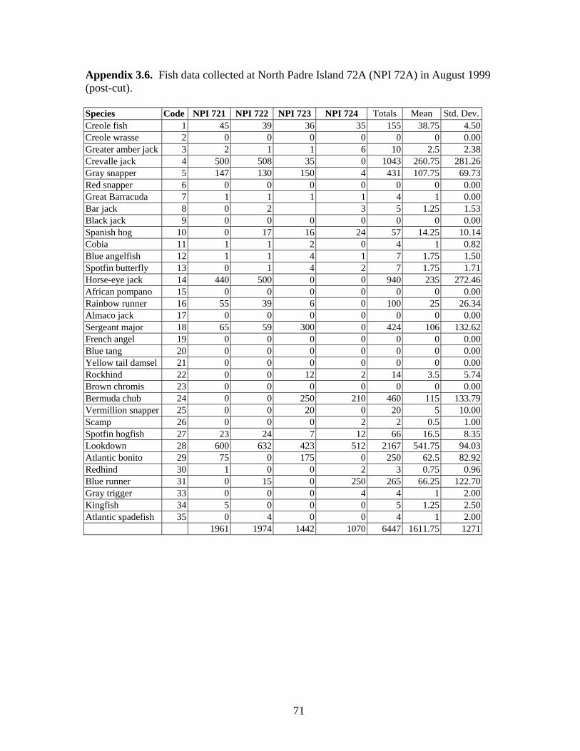
Appendix 3.6. Fish data collected at North Padre Island 72A (NPI 72A) in August 1999 (post-cut).
Species Code NPI 721 NPI 722 NPI 723 NPI 724 Totals Mean Std. Dev.Creole fish 1 45 39 36 35 155 38.75 4.50Creole wrasse 2 0 0 0 0 0 0 0.00Greater amber jack 3 2 1 1 6 10 2.5 2.38Crevalle jack 4 500 508 35 0 1043 260.75 281.26Gray snapper 5 147 130 150 4 431 107.75 69.73Red snapper 6 0 0 0 0 0 0 0.00Great Barracuda 7 1 1 1 1 4 1 0.00Bar jack 8 0 2 3 5 1.25 1.53Black jack 9 0 0 0 0 0 0 0.00Spanish hog 10 0 17 16 24 57 14.25 10.14Cobia 11 1 1 2 0 4 1 0.82Blue angelfish 12 1 1 4 1 7 1.75 1.50Spotfin butterfly 13 0 1 4 2 7 1.75 1.71Horse-eye jack 14 440 500 0 0 940 235 272.46African pompano 15 0 0 0 0 0 0 0.00Rainbow runner 16 55 39 6 0 100 25 26.34Almaco jack 17 0 0 0 0 0 0 0.00Sergeant major 18 65 59 300 0 424 106 132.62French angel 19 0 0 0 0 0 0 0.00Blue tang 20 0 0 0 0 0 0 0.00Yellow tail damsel 21 0 0 0 0 0 0 0.00Rockhind 22 0 0 12 2 14 3.5 5.74Brown chromis 23 0 0 0 0 0 0 0.00Bermuda chub 24 0 0 250 210 460 115 133.79Vermillion snapper 25 0 0 20 0 20 5 10.00Scamp 26 0 0 0 2 2 0.5 1.00Spotfin hogfish 27 23 24 7 12 66 16.5 8.35Lookdown 28 600 632 423 512 2167 541.75 94.03Atlantic bonito 29 75 0 175 0 250 62.5 82.92Redhind 30 1 0 0 2 3 0.75 0.96Blue runner 31 0 15 0 250 265 66.25 122.70Gray trigger 33 0 0 0 4 4 1 2.00Kingfish 34 5 0 0 0 5 1.25 2.50Atlantic spadefish 35 0 4 0 0 4 1 2.00
1961 1974 1442 1070 6447 1611.75 1271
71
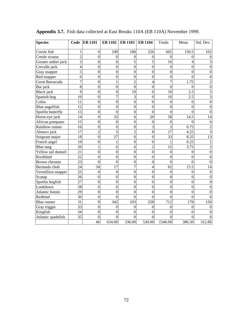
Appendix 3.7. Fish data collected at East Breaks 110A (EB 110A) November 1999.
Species Code EB 1101 EB 1102 EB 1103 EB 1104 Totals Mean Std. Dev.
Creole fish 1 0 190 186 226 602 150.5 102Creole wrasse 2 0 0 0 0 0 0 0Greater amber jack 3 0 6 5 5 16 4 3Crevalle jack 4 0 0 0 0 0 0 0Gray snapper 5 0 0 0 0 0 0 0Red snapper 6 0 0 0 0 0 0 0Great Barracuda 7 0 1 2 4 7 1.75 2Bar jack 8 0 0 0 0 0 0 0Black jack 9 0 0 10 0 10 2.5 5Spanish hog 10 0 7 3 0 10 2.5 3Cobia 11 0 0 0 0 0 0 0Blue angelfish 12 0 0 0 0 0 0 0Spotfin butterfly 13 0 0 0 0 0 0 0Horse-eye jack 14 0 32 6 20 58 14.5 14African pompano 15 0 0 0 0 0 0 0Rainbow runner 16 0 0 0 3 3 0.75 2Almaco jack 17 2 5 2 8 17 4.25 3Sergeant major 18 0 27 6 0 33 8.25 13French angel 19 0 1 0 0 1 0.25 1Blue tang 20 1 6 6 2 15 3.75 3Yellow tail damsel 21 0 0 0 0 0 0 0Rockhind 22 0 0 0 0 0 0 0Brown chromis 23 0 0 0 0 0 0 0Bermuda chub 24 34 17 7 4 62 15.5 14Vermillion snapper 25 0 0 0 0 0 0 0Scamp 26 0 0 0 0 0 0 0Spotfin hogfish 27 0 0 0 0 0 0 0Lookdown 28 0 0 0 0 0 0 0Atlantic bonito 29 0 0 0 0 0 0 0Redhind 30 0 0 0 0 0 0 0Blue runner 31 9 342 103 258 712 178 150Gray trigger 33 0 0 0 0 0 0 0Kingfish 34 0 0 0 0 0 0 0Atlantic spadefish 35 0 0 0 0 0 0 0
46 634.00 336.00 530.00 1546.00 386.50 312.86
72
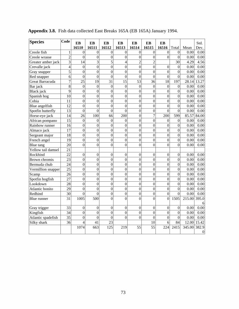
Appendix 3.8. Fish data collected East Breaks 165A (EB 165A) January 1994.
Species Code EB 16510
EB 16511
EB 16512
EB 16513
EB 16514
EB 16515
EB 16516 Total Mean
Std. Dev.
Creole fish 1 0 0 0 0 0 0 0 0 0.00 0.00Creole wrasse 2 0 0 0 0 0 0 0 0 0.00 0.00Greater amber jack 3 14 3 5 4 2 2 30 4.29 4.56Crevalle jack 4 0 0 0 0 0 0 0 0 0.00 0.00Gray snapper 5 0 0 0 0 0 0 0 0 0.00 0.00Red snapper 6 0 0 0 0 0 0 0 0 0.00 0.00Great Barracuda 7 25 19 31 15 53 36 18 197 28.14 13.27Bar jack 8 0 0 0 0 0 0 0 0 0.00 0.00Black jack 9 0 0 0 0 0 0 0 0 0.00 0.00Spanish hog 10 0 0 0 0 0 0 0 0 0.00 0.00Cobia 11 0 0 0 0 0 0 0 0 0.00 0.00Blue angelfish 12 0 0 0 0 0 0 0 0 0.00 0.00Spotfin butterfly 13 0 0 0 0 0 0 0 0 0.00 0.00Horse-eye jack 14 26 100 66 200 0 7 200 599 85.57 84.00African pompano 15 0 0 0 0 0 0 0 0 0.00 0.00Rainbow runner 16 0 0 0 0 0 0 0 0 0.00 0.00Almaco jack 17 0 0 0 0 0 0 0 0 0.00 0.00Sergeant major 18 0 0 0 0 0 0 0 0 0.00 0.00French angel 19 0 0 0 0 0 0 0 0 0.00 0.00Blue tang 20 0 0 0 0 0 0 0 0 0.00 0.00Yellow tail damsel 21 Rockhind 22 0 0 0 0 0 0 0 0 0.00 0.00Brown chromis 23 0 0 0 0 0 0 0 0 0.00 0.00Bermuda chub 24 0 0 0 0 0 0 0 0 0.00 0.00Vermillion snapper 25 0 0 0 0 0 0 0 0 0.00 0.00Scamp 26 0 0 0 0 0 0 0 0 0.00 0.00Spotfin hogfish 27 0 0 0 0 0 0 0 0 0.00 0.00Lookdown 28 0 0 0 0 0 0 0 0 0.00 0.00Atlantic bonito 29 0 0 0 0 0 0 0 0 0.00 0.00Redhind 30 0 0 0 0 0 0 0 0 0.00 0.00Blue runner 31 1005 500 0 0 0 0 0 1505 215.00 395.0
6Gray trigger 33 0 0 0 0 0 0 0 0 0.00 0.00Kingfish 34 0 0 0 0 0 0 0 0 0.00 0.00Atlantic spadefish 35 0 0 0 0 0 0 0 0 0.00 0.00Silky shark 36 4 41 23 10 6 84 12.00 15.42
1074 663 125 219 55 55 224 2415 345.00 382.90
73
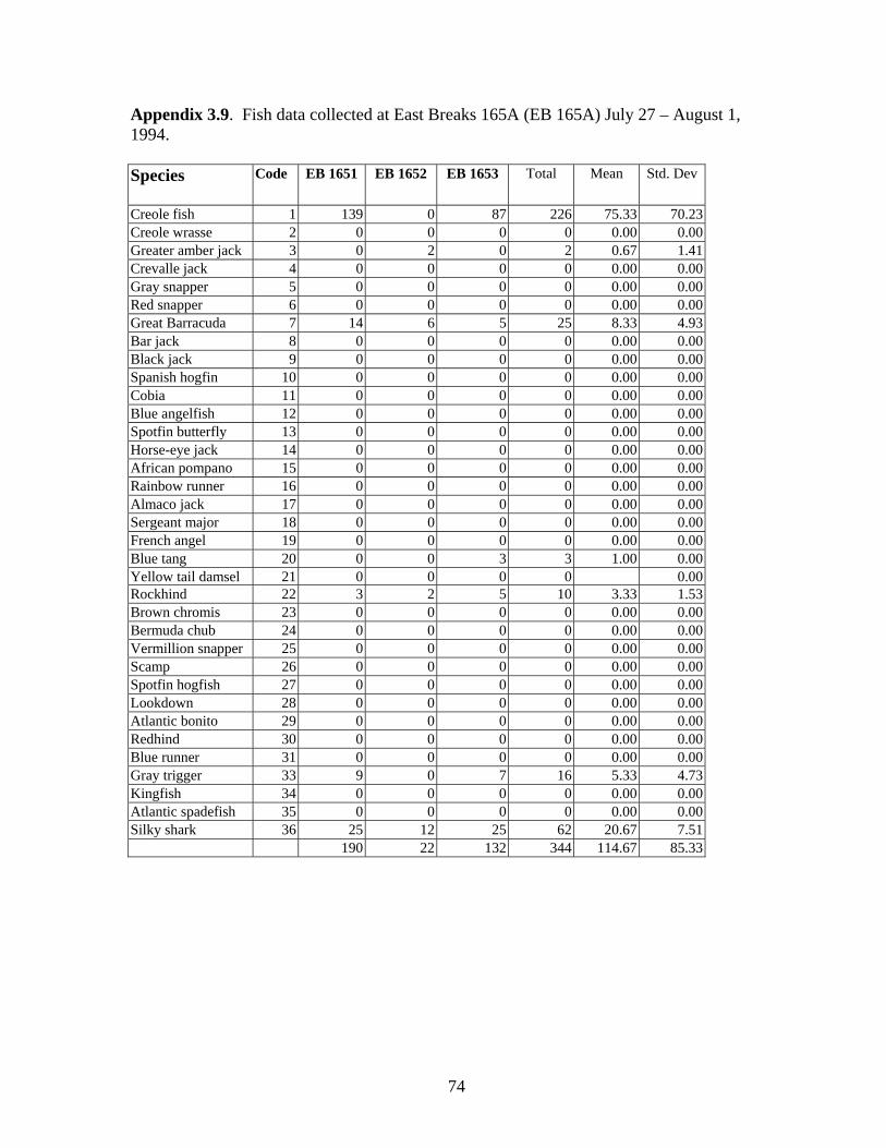
Appendix 3.9. Fish data collected at East Breaks 165A (EB 165A) July 27 – August 1, 1994. Species Code EB 1651 EB 1652 EB 1653 Total Mean Std. Dev
Creole fish 1 139 0 87 226 75.33 70.23 Creole wrasse 2 0 0 0 0 0.00 0.00 Greater amber jack 3 0 2 0 2 0.67 1.41 Crevalle jack 4 0 0 0 0 0.00 0.00 Gray snapper 5 0 0 0 0 0.00 0.00 Red snapper 6 0 0 0 0 0.00 0.00 Great Barracuda 7 14 6 5 25 8.33 4.93 Bar jack 8 0 0 0 0 0.00 0.00 Black jack 9 0 0 0 0 0.00 0.00 Spanish hogfin 10 0 0 0 0 0.00 0.00 Cobia 11 0 0 0 0 0.00 0.00 Blue angelfish 12 0 0 0 0 0.00 0.00 Spotfin butterfly 13 0 0 0 0 0.00 0.00 Horse-eye jack 14 0 0 0 0 0.00 0.00 African pompano 15 0 0 0 0 0.00 0.00 Rainbow runner 16 0 0 0 0 0.00 0.00 Almaco jack 17 0 0 0 0 0.00 0.00 Sergeant major 18 0 0 0 0 0.00 0.00 French angel 19 0 0 0 0 0.00 0.00 Blue tang 20 0 0 3 3 1.00 0.00 Yellow tail damsel 21 0 0 0 0 0.00 Rockhind 22 3 2 5 10 3.33 1.53 Brown chromis 23 0 0 0 0 0.00 0.00 Bermuda chub 24 0 0 0 0 0.00 0.00 Vermillion snapper 25 0 0 0 0 0.00 0.00 Scamp 26 0 0 0 0 0.00 0.00 Spotfin hogfish 27 0 0 0 0 0.00 0.00 Lookdown 28 0 0 0 0 0.00 0.00 Atlantic bonito 29 0 0 0 0 0.00 0.00 Redhind 30 0 0 0 0 0.00 0.00 Blue runner 31 0 0 0 0 0.00 0.00 Gray trigger 33 9 0 7 16 5.33 4.73 Kingfish 34 0 0 0 0 0.00 0.00 Atlantic spadefish 35 0 0 0 0 0.00 0.00 Silky shark 36 25 12 25 62 20.67 7.51
190 22 132 344 114.67 85.33
74
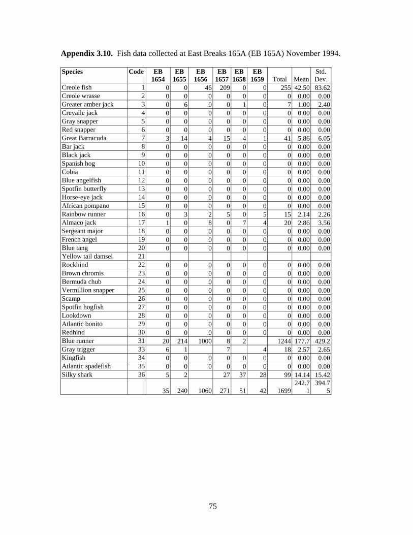
Appendix 3.10. Fish data collected at East Breaks 165A (EB 165A) November 1994.
Species Code EB 1654
EB 1655
EB 1656
EB 1657
EB 1658
EB 1659 Total Mean
Std. Dev.
Creole fish 1 0 0 46 209 0 0 255 42.50 83.62 Creole wrasse 2 0 0 0 0 0 0 0 0.00 0.00 Greater amber jack 3 0 6 0 0 1 0 7 1.00 2.40 Crevalle jack 4 0 0 0 0 0 0 0 0.00 0.00 Gray snapper 5 0 0 0 0 0 0 0 0.00 0.00 Red snapper 6 0 0 0 0 0 0 0 0.00 0.00 Great Barracuda 7 3 14 4 15 4 1 41 5.86 6.05 Bar jack 8 0 0 0 0 0 0 0 0.00 0.00 Black jack 9 0 0 0 0 0 0 0 0.00 0.00 Spanish hog 10 0 0 0 0 0 0 0 0.00 0.00 Cobia 11 0 0 0 0 0 0 0 0.00 0.00 Blue angelfish 12 0 0 0 0 0 0 0 0.00 0.00 Spotfin butterfly 13 0 0 0 0 0 0 0 0.00 0.00 Horse-eye jack 14 0 0 0 0 0 0 0 0.00 0.00 African pompano 15 0 0 0 0 0 0 0 0.00 0.00 Rainbow runner 16 0 3 2 5 0 5 15 2.14 2.26 Almaco jack 17 1 0 8 0 7 4 20 2.86 3.56 Sergeant major 18 0 0 0 0 0 0 0 0.00 0.00 French angel 19 0 0 0 0 0 0 0 0.00 0.00 Blue tang 20 0 0 0 0 0 0 0 0.00 0.00 Yellow tail damsel 21 Rockhind 22 0 0 0 0 0 0 0 0.00 0.00 Brown chromis 23 0 0 0 0 0 0 0 0.00 0.00 Bermuda chub 24 0 0 0 0 0 0 0 0.00 0.00 Vermillion snapper 25 0 0 0 0 0 0 0 0.00 0.00 Scamp 26 0 0 0 0 0 0 0 0.00 0.00 Spotfin hogfish 27 0 0 0 0 0 0 0 0.00 0.00 Lookdown 28 0 0 0 0 0 0 0 0.00 0.00 Atlantic bonito 29 0 0 0 0 0 0 0 0.00 0.00 Redhind 30 0 0 0 0 0 0 0 0.00 0.00 Blue runner 31 20 214 1000 8 2 1244 177.7 429.2 Gray trigger 33 6 1 7 4 18 2.57 2.65 Kingfish 34 0 0 0 0 0 0 0 0.00 0.00 Atlantic spadefish 35 0 0 0 0 0 0 0 0.00 0.00 Silky shark 36 5 2 27 37 28 99 14.14 15.42
35 240 1060 271 51 42 1699
242.71
394.75
75