Characteristic Signatures of Vector Fields during Inflation

Characteristic Signatures of Vector Fields duringInflation

Ryo Namba

School of Physics and AstronomyUniversity of Minnesota

IPMU Seminar: September 6, 2012

N. Barnaby, RN & M. Peloso, Phys. Rev. D 85, 123523 (2012) [arXiv:1202.1469].RN, [arXiv:1207.5547].

Ryo Namba (UMN) Vector Fields IPMU 2012 1 / 29

Outline

1 Introduction

2 Nearly Local Non-gaussianity from Dilaton-like Kinetic Coupling

3 Statistical Anisotropy from Massive Vector Curvaton

4 Conclusion and Future Prospects


Outline

1 Introduction





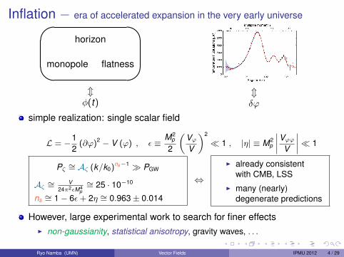
Inflation − era of accelerated expansion in the very early universe�

�

�

�horizon

monopole flatness

mφ(t)

mδϕ

simple realization: single scalar field

L = −12

(∂ϕ)2 − V (ϕ) , ε ≡M2

p

2

(VϕV

)2

� 1 , |η| ≡ M2p

∣∣∣∣VϕϕV

∣∣∣∣� 1

Pζ ∼= Aζ (k/k0)ns−1 � PGW

Aζ ∼= V24π2εM4

p

∼= 25 · 10−10

ns ∼= 1− 6ε+ 2η ∼= 0.963± 0.014

⇔

I already consistentwith CMB, LSS

I many (nearly)degenerate predictions

However, large experimental work to search for finer effectsI non-gaussianity, statistical anisotropy, gravity waves, . . .


Non-gaussianity⇔ Interactions

Claimed: f localNL = 48± 20 (1σ) Xia, Baccigalupi, Matarrese, Verde & Viel ’11

Planck forecast − f localNL ∼ 5− 10

1000500200 2000300 300015007001

2

345

10

20

lmax

Df N

L

Local model

WMAP HT�T+PLPlanck HT�T+PL

CMBPol HT�T+PL

Liguori, Sefusatti, Fergusson & Shellard ’10

Simplest models→ unobservable NG: f localNL ∼ O

(10−2

)Statistical anisotropy⇔ Broken rotational invariance

Claimed: g∗ = 0.29± 0.031 Groeneboom, Ackerman, Wehus & Eriksen ’09

This apparent broken stat. isotropy is most likely systematic.

Planck will probe g∗ ∼ O(10−2

)Pullen & Kamionkowski ’07


Vector fields cansource a very distinctive non-gaussianity

break rotational invariance→ give stat. anisotropy

In this talk,

Dilatonic Coupling

Lint = − I2(ϕ)

4F 2

U(1) gauge field

approximate local NG

quadrupolar sign. of spin 1 origin

Barnaby , RN & Peloso ’12

Massive Vector Curvaton

Lcurv = − f (ϕ)

4F 2 − 1

2m2(ϕ)A2

no gauge symmetry

statistically isotropic spectrum ?

independent of forms of f & m ?

RN ’12


Outline

1 Introduction





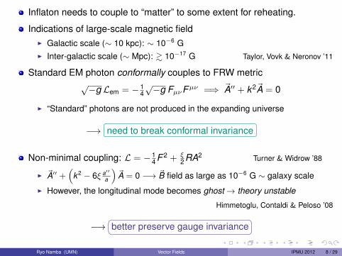
Inflaton needs to couple to “matter” to some extent for reheating.

Indications of large-scale magnetic fieldI Galactic scale (∼ 10 kpc): ∼ 10−6 GI Inter-galactic scale (∼ Mpc): & 10−17 G Taylor, Vovk & Neronov ’11

Standard EM photon conformally couples to FRW metric√−g Lem = − 1

4√−g FµνFµν =⇒ ~A′′ + k2~A = 0

I “Standard” photons are not produced in the expanding universe

−→�� need to break conformal invariance

Non-minimal coupling: L = − 14 F 2 + ξ

2 RA2 Turner & Widrow ’88

I ~A′′ +(

k2 − 6ξ a′′a

)~A = 0 −→ ~B field as large as 10−6 G ∼ galaxy scale

I However, the longitudinal mode becomes ghost→ theory unstable

Himmetoglu, Contaldi & Peloso ’08

−→�� better preserve gauge invariance


Break conformal, preserve gauge invariance

L = − I2(t)4

F 2 , I ∝ an Ratra ’91

Large-scale ~B field⇔ scale-inv. ~B spectra preferable =⇒ n = −3,2n = −3 leads to ρgauge � ρinflaton

I Inflation still continues, but too small ~B field. Kanno, Soda & Watanabe ’09

Let’s take n = 2

“Magnetic” & “electric” spectra:

dd ln k

⟨~B2⟩ ∼ H4 � d

d ln k⟨~E2⟩ ∼ H4

(k

aH

)2

, after hor. cross.

In FT,External function ⇔ Vacuum condensate of field(s)

I(t) ⇔ I [φ(t)]

↪→ inflaton


Model of Dilatonic Coupling

S =

∫d4x√−g[−1

2∂µϕ∂

µϕ− V (ϕ)− I2(ϕ)

4FµνFµν

]Effective “charge”: eeff = e0/I [φ(t)]

�

�

�

�No vector VEV

Isotropic bckgnd

ϕ(x) = φ(t) + δϕ(x)

Time dependence dynamically achieved

V = µ4−rϕr , I = Iend exp(− nϕ2

2 r M2p

), n = 2

However . . .

eeff ∝ I−1 ∝ a−2 =⇒ eend ≤ e120einDemozzi, Mukhanov& Rubinstein ’09

1 eeff = eem at the end⇒ Strong coupling

2 eeff . O(1) initially⇒ Aµ 6= photon

eEM

tendt

eeff


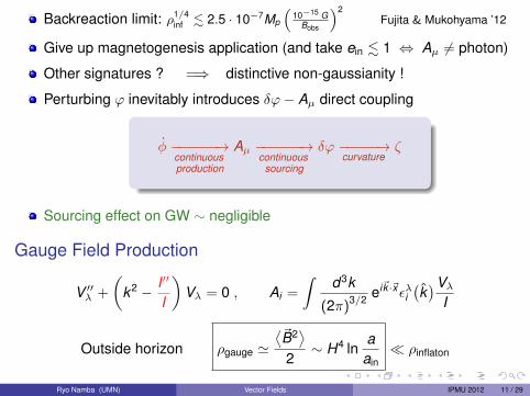
Backreaction limit: ρ1/4inf . 2.5 · 10−7Mp

(10−15 G

Bobs

)2Fujita & Mukohyama ’12

Give up magnetogenesis application (and take ein . 1 ⇔ Aµ 6= photon)

Other signatures ? =⇒ distinctive non-gaussianity !

Perturbing ϕ inevitably introduces δϕ− Aµ direct coupling

φ −−−−−−→continuousproduction

Aµ −−−−−−→continuous

sourcing

δϕ −−−−−→curvature

ζ

Sourcing effect on GW ∼ negligible

Gauge Field Production

V ′′λ +

(k2 − I′′

I

)Vλ = 0 , Ai =

∫d3k

(2π)3/2 ei~k·~xελi(k)Vλ

I

Outside horizon ρgauge '⟨~B2⟩

2∼ H4 ln

aain� ρinflaton


Produced gauge quanta source δϕ[∂2τ + 2

a′

a∂τ −∇2 + a2Vϕϕ

]δϕ =

a2

2I2ϕ

I2

(~E2 − ~B2

)︸︷︷︸

≡Jϕ

+ . . .

Solution consists of 2 uncorrelated parts:

δϕ = δϕvac︸︷︷︸homogeneous

+ δϕsourced︸︷︷︸particular

δϕvac ∼ H/ (2π)→ standard vacuum solution

δϕsourced(τ, ~k)

=∫ τ dτ ′Gk (τ, τ ′)︸︷︷︸

constructedfrom δϕvac

Jϕ(τ ′, ~k

)︸︷︷︸operator

in Fourier space

δϕsourced ∝ (Aµ)2 =⇒ highly NG !


Two-point correlator⟨δϕ(~k1)δϕ(~k2)⟩

=⟨δϕvac

(~k1)δϕvac

(~k2)⟩

+⟨δϕsourced

(~k1)δϕsourced

(~k2)⟩

⟨δϕsourced

(~k1)δϕsourced

(~k2)⟩

=∫ τ dτ1dτ2 Gk1 (τ, τ1)Gk2 (τ, τ2)

⟨Jϕ(τ1, ~k1)Jϕ(τ2, ~k2)

⟩I Two pieces are uncorrelated 〈δϕvacδϕsourced〉 = 0.

Three-point correlator⟨δϕ(~k1)δϕ(~k2)δϕ(~k3)⟩'⟨δϕsourced

(~k1)δϕsourced

(~k2)δϕsourced

(~k3)⟩∼⟨J3ϕ

⟩I Contribution from vacuum is undetectable.

Curvature perturbation : ζ = −Hφδϕ

Power spectrum: Pζ = Pvac + Psourced ∼⟨δϕ2

vac⟩

+⟨δϕ2

sourced

⟩Vacuum term dominates→ Pvac > Psourced → Ntot − NCMB < 580

(60

NCMB

)2


Bispectrum

Bζ (k1, k2, k3) δ(3)(~k1 + ~k2 + ~k3

)=⟨ζ~k1ζ~k2ζ~k3

⟩'(−Hφ

)3 ⟨δϕ3

sourced⟩

~k1 + ~k2 + ~k3 = 0→ forms a triangle

Features in Bζ (k1, k2, k3)

1 Shape: relative shape of the triangleI squeezed, equilateral, flattened

2 Amplitude: magnitude at a given shape⇔ fNL ∼ BζP2ζ

3 Running: dependence on the overall size of the triangle

∗ fNL: deviation from Gaussian statistics Komatsu & Spergel ’00

Local ansatz : Φ = Φg + fNL(Φ2

g −⟨Φ2

g⟩)

, ζ ∼ Φ

−10 < f localNL < 74, −214 < f equil

NL < 266, −410 < f orthNL < 6 95% CL WMAP7


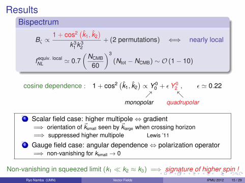
ResultsBispectrum

Bζ ∝1 + cos2

(k1, k2

)k3

1 k32

+ (2 permutations) ⇐⇒ nearly local

f equiv. localNL ' 0.7

(NCMB

60

)3

(Ntot − NCMB) ∼ O (1− 10)

cosine dependence : 1 + cos2 (k1, k2)∝ Y 0

0 + εY 02 , ε ' 0.22

↗ ↖monopolar quadrupolar

1 Scalar field case: higher multipole⇔ gradient=⇒ orientation of ~ksmall seen by ~klarge when crossing horizon=⇒ suppressed higher multipole Lewis ’11

2 Gauge field case: angular dependence⇔ polarization operator=⇒ non-vanishing for ksmall → 0

Non-vanishing in squeezed limit (k1 � k2 ≈ k3) =⇒ signature of higher spin !Ryo Namba (UMN) Vector Fields IPMU 2012 15 / 29

Outline

1 Introduction





Statistical anisotropy

ACW parametrization : Pζ = Piso

[1 + g∗

(n · k

)2]

Assumed: 2D symmetry & parity

g∗ = 0.10± 0.04 g∗ = 0.15± 0.04Groeneboom & Eriksen 2008

Increase of significance with ` Pullen & Kamionkowski 2007


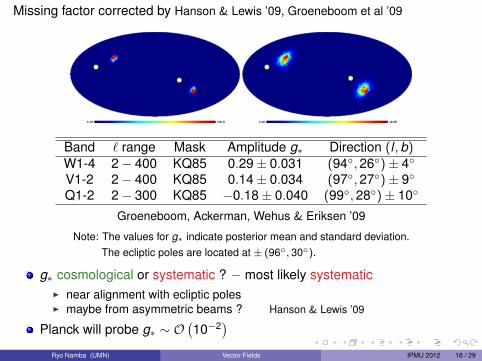
Missing factor corrected by Hanson & Lewis ’09, Groeneboom et al ’09

Band ` range Mask Amplitude g∗ Direction (l ,b)W1-4 2− 400 KQ85 0.29± 0.031 (94◦,26◦)± 4◦

V1-2 2− 400 KQ85 0.14± 0.034 (97◦,27◦)± 9◦

Q1-2 2− 300 KQ85 −0.18± 0.040 (99◦,28◦)± 10◦

Groeneboom, Ackerman, Wehus & Eriksen ’09

Note: The values for g∗ indicate posterior mean and standard deviation.The ecliptic poles are located at ± (96◦, 30◦).

g∗ cosmological or systematic ? − most likely systematicI near alignment with ecliptic polesI maybe from asymmetric beams ? Hanson & Lewis ’09

Planck will probe g∗ ∼ O(10−2

)Ryo Namba (UMN) Vector Fields IPMU 2012 18 / 29

Anisotropic inflationVector curvaton

}−→ g∗

Rapid isotropization for Bianchi spaces with Λ + Tµν satisfying thedominant and strong energy conditions Wald ’83

Counterexamples − breaking the premises of above theorem1 Kalb-Ramond axion (Kaloper ’91)

2 higher curvature terms (Barrow & Hervik ’05)

3 Non-minimal vector fieldsF Potential term: V

(A2) Ford ’89

F Fixed norm: λ(A2 − v2) ACW ’07

F Non-minimal coupling: R A2 Golovnev, Mukhanov & Vanchurin ’08

⇓All these suffer ghost instabilities Himmetoglu, Contaldi & Peloso ’08

Prolonged anisotropy: f 2 F 2 with suitable f Watanabe, Kanno & Soda ’09


Vector CurvatonVector curvaton: L = − f (t)

4 F 2 − 12 m2(t)A2 Dimopoulos, Karciauskas & Wagstaff ’09

No ghosts for f ,m2 > 0Scale-inv. & stat. isotropic spectrum in curvaton mechanism if

I f ∝ a−4, m ∝ aI Vector is light initially & heavy at the end of inflationI Equipartition between initial vector kinetic & potential energy

under the simplifying assumptions of . . .External functions f (t) & m(t)Isotropic de Sitter background

However . . . RN ’12

Time dependence⇔ vacuum condensate of some field

Min. implementation: f (t),m(t)→ f (ϕ),m(ϕ)

I ϕ: inflaton↔ physical clock

f ,m nontrivial evolution→ field cannot be integrated out(i.e. its fluctuations cannot be ignored)


Model of Massive Vector Curvaton Dimopoulos, Karciauskas & Wagstaff ’09RN ’12

S =

∫d4x√−g[−1

2∂µϕ∂

µϕ− V (ϕ)− f (ϕ)

4FµνFµν − 1

2m2(ϕ)AµAµ

]↗ ↖

inflaton sector vector curvaton sector

VEV: A(0)µ = (0,A,0,0) − background orientation

Perturbation: δAµ − no gauge freedom

Only δAµ in Dimopoulos, Karciauskas & Wagstaff ’09, here also δϕ included

1 φ(t)→ Expansion mostly driven by V [φ(t)]

2 A(0)µ (t)→ breaks the background isotropy

ds2 = −dt2 + a2(t) dx2 + b2(t)(dy2 + dz2) , a = eα−2σ, b = eα+σ

3 Suitable choice dynamically achieves f ∝ a−4, m ∝ a by φ(t) motion

V (ϕ) =12

m2ϕϕ

2 =⇒ f (ϕ) = exp(

c ϕ2

M2p

), m(ϕ) = m0 exp

(− c ϕ2

4M2p

)−→ inevitably introduces δϕ− δAµ interaction at linearized level


Background Dynamics & AttractorThree physical scales:

1 Physical momentum: k/a

2 “Overall” Hubble parameter: H ≡ α3 “Physical” vector mass: M ≡ m/

√f

Attractor solution − valid for c > 1

I achieves the desired f ∝ a−4 and m ∝ a

I fixes φ, ρA/ρφ, σ/α = ∆H/H

heavybecomes

vector

horizoncrossing

Mk � a

H

t

-60 -40 -20 0

-4

-2

0

Α

f �f

Α vector ® heavy

-60 -40 -20 010-3

10-2

10-1

1

Α

ΡA

�ΡΦ

end of inf .analyticalnumerical

-60 -40 -20 010-6

10-4

10-2

Α

Σ �Α

vector ® heavyanalyticalnumerical


Perturbations

Residual 2D symmetry→ ~k = (kL, kT ,0)

d.o.f: δAµ + δϕ+ (no δgµν) = total 5 d.o.f2D vector: δAz −→ no contribution to ζ at linearized levell decoupled

2D scalar: δA0+�� δAx + δAy + δϕ −(non dynamical δA0) = 3 d.o.f

Quantization − in matrix form1 Diagonalize Hamiltonian: ψi = Rij δj , δi = (δϕ, δAx , δAy )i

H = 12

∫d3k

[π†π + ψ†ω2ψ

], ω2 : diagonal

2 Quantize:

ψi(t , ~k)

= hij(t , ~k)

aj(~k)

+ h.c. , πi(t , ~k)

= hij(t , ~k)

aj(~k)

+ h.c.

3 Bogolyubov: h = 1√2ω

(α + β) , h = −i ω√2ω

(α− β)

4 Adiabatic initial no-particle state → αin = e−i∫ tin dt ω , βin = 0


Curvaton Mechanism1 ρA ∼ constant during inflation.2 Inflaton decays into rad. after inflation.3 Then δρA︸︷︷︸

∝a−3

� δρr︸︷︷︸∝a−4

4 Isocurvature→ curvature conversionheavy

Vectorbecomes

End of inf

Inflaton decay

∆ΡA

∆Ρr

∆ΡΦ

time

ζ = −Hδρ

ρ' r

4 + 3r︸︷︷︸magnitude

δρA

ρA, r ≡ ρA

ρr Lyth & Wands ’02

∗ r “only” determines the normalization∗ Features (scale dependence, stat. (an)isotropy) in spectrum⇔ δρA

ρA≡ δ

∗ At late times, gradient is negligible

δρlateA ' f

a2

[A δAx + M2A δAx

]Power spec. :

⟨δ(~x)δ(~y)⟩

=

∫dkk

∫ 1

0dξ cos (k ξ rL) J0

(k√

1− ξ2 rT

)Pδ(k , ξ)


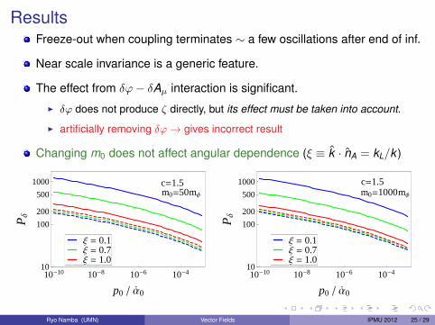
ResultsFreeze-out when coupling terminates ∼ a few oscillations after end of inf.

Near scale invariance is a generic feature.

The effect from δϕ− δAµ interaction is significant.

I δϕ does not produce ζ directly, but its effect must be taken into account.

I artificially removing δϕ→ gives incorrect result

Changing m0 does not affect angular dependence (ξ ≡ k · nA = kL/k )

10-10 10-8 10-6 10-410

100

200

500

1000

p0 � Α 0

P∆

Ξ = 1.0Ξ = 0.7Ξ = 0.1

m0=50mΦ

c=1.5

10-10 10-8 10-6 10-410

100

200

500

1000

p0 � Α 0

P∆

Ξ = 1.0Ξ = 0.7Ξ = 0.1

m0=1000mΦ

c=1.5


Instead, changing c makes significant impact (recall: f ,m ∼ ec ϕ2)

I g∗ = g∗ (c)

m0=1000mΦ

1.05 1.1 1.2 1.3 1.4-0.8-0.6-0.4-0.2

00.20.4

c

g *

∗ Anisotropy is produced & encoded when λ ∼ M−1

∗ g∗ . 0.1 can be achieved, but requires fine-tuning

∗ The level of stat. anisotropy is a function of the functional forms of f & m,not only on their time dependence.


Outline

1 Introduction





Concluding Remarks

Vector fields←→ Distinctive phenomenology

Non-gaussianity

Model: dilaton-like kinetic coupling Lint = − 14 I2F 2

Aµ production→ source ζ ∼ highly NG

Bζ ∝ 1+cos2(k1·k2)

k31 k3

2, f equiv.local

NL ∼ O (1− 10)

Difficult realization of primordial magnetogenesis

Statistical anisotropy

Model: Massive vector curvaton Lcurv = − 14 f F 2 − 1

2 m2A2

No ghost instabilities with appropriate kinetic & mass functions

Anisotropy encoded in the spectrum in the early stage of inflation

g∗ . 0.1 is possible but requires fine-tuning.


Future ProspectOngoing work:

Running non-gaussianity when I ∝ an in the dilatonic coupling model

n = 2 −→ fNL ∝ N3CMB (Ntot − NCMB)

N3CMB →

3∏i=1

[(aH/ki )

2(n−2) − 1n − 2

], Ntot − NCMB →

(K/ainH)2(n−2) − 1n − 2

Chiral GW at interferometersI Axioninc coupling b/w ϕ & Aµ

Lint = − α4fϕFµν Fµν

I Parity violating Lint → chiral GW, PGWR � PGW

L

I ∆χ ≡ PGWR −PGW

LPGW

R +PGWL

?? Magnetogenesis from inflation ??Ryo Namba (UMN) Vector Fields IPMU 2012 29 / 29

Characteristic Signatures of Vector Fields during Inflation

Documents

Transcript of Characteristic Signatures of Vector Fields during Inflation