Chapters 5-7 Correlation/Linear Regression
47
1 Chapters 5-7 Correlation/Linear Regression • Linear Relationships: If the explanatory and response variables show a straight-line pattern, then we say they follow a linear relationship. • Curved relationships and clusters are other forms to watch for.
description
Chapters 5-7 Correlation/Linear Regression. Linear Relationships: If the explanatory and response variables show a straight-line pattern, then we say they follow a linear relationship. Curved relationships and clusters are other forms to watch for. Chapters 5-7 Correlation/Linear Regression. - PowerPoint PPT Presentation
Transcript of Chapters 5-7 Correlation/Linear Regression

1
Chapters 5-7 Correlation/Linear Regression
• Linear Relationships: If the explanatory and response variables show a straight-line pattern, then we say they follow a linear relationship.
• Curved relationships and clusters are other forms to watch for.
2
Chapters 5-7 Correlation/Linear Regression
• Linear Relationships: If the explanatory and response variables show a straight-line pattern, then we say they follow a linear relationship.
• Curved relationships and clusters are other forms to watch for.
3
Chapters 5-7 Correlation/Linear Regression
• Direction: If the relationship has a clear direction, we speak of either positive association or negative association.
• Positive association: high values of the two variables tend to occur together
• Negative association: high values of one variable tend to occur with low values of the other variable.
4
Chapters 5-7 Correlation/Linear Regression
• Correlation is a number that determines the strength of a linear relationship between two quantitative variables.
• Correlation is always between -1 and 1 inclusive
• The sign of a correlation coefficient determines positive/negative association between the variables
5
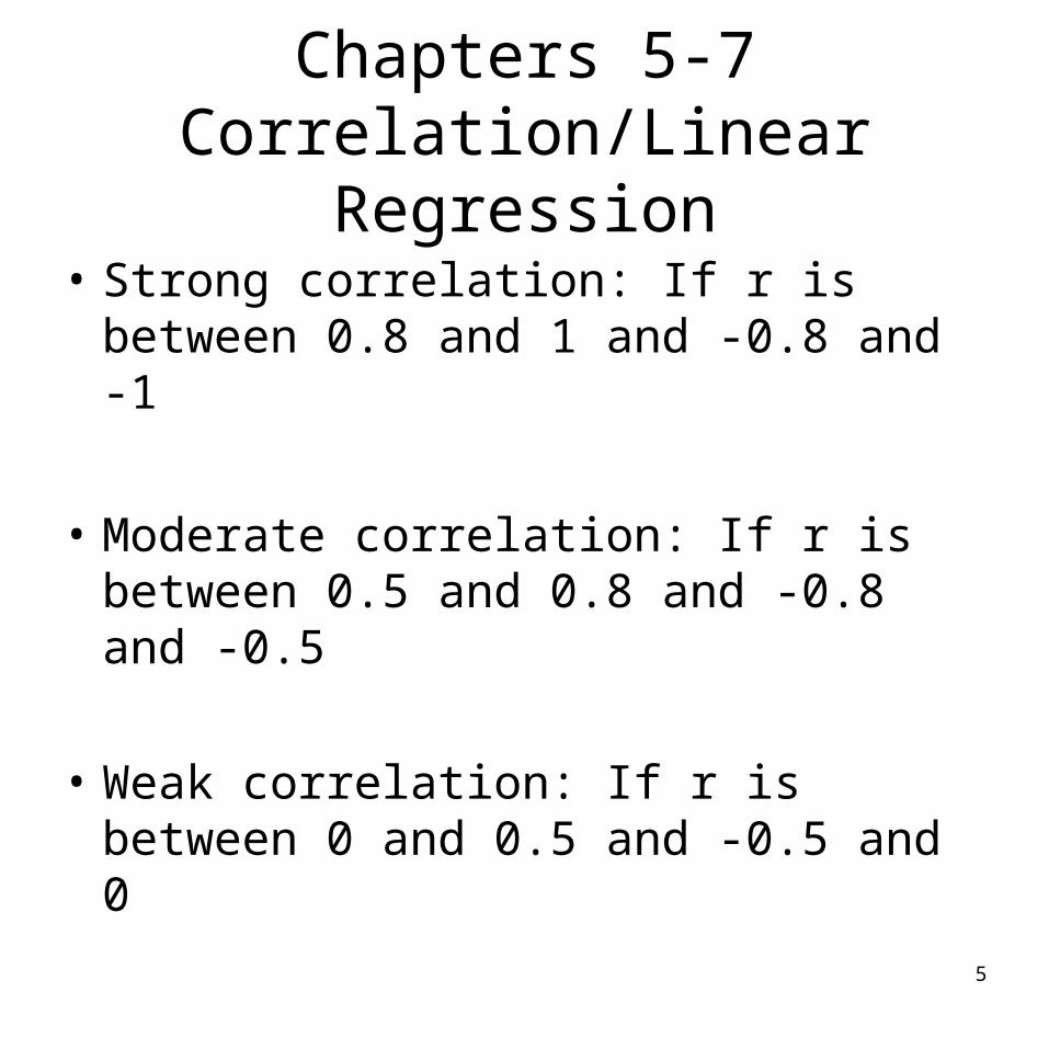
Chapters 5-7 Correlation/Linear Regression
• Strong correlation: If r is between 0.8 and 1 and -0.8 and -1
• Moderate correlation: If r is between 0.5 and 0.8 and -0.8 and -0.5
• Weak correlation: If r is between 0 and 0.5 and -0.5 and 0
6
Chapters 5-7 Correlation/Linear Regression
• Correlation does not distinguish between X and Y
• Correlation is unitless
• Correlation measures the strength of linear relationship between two quantitative variables
7
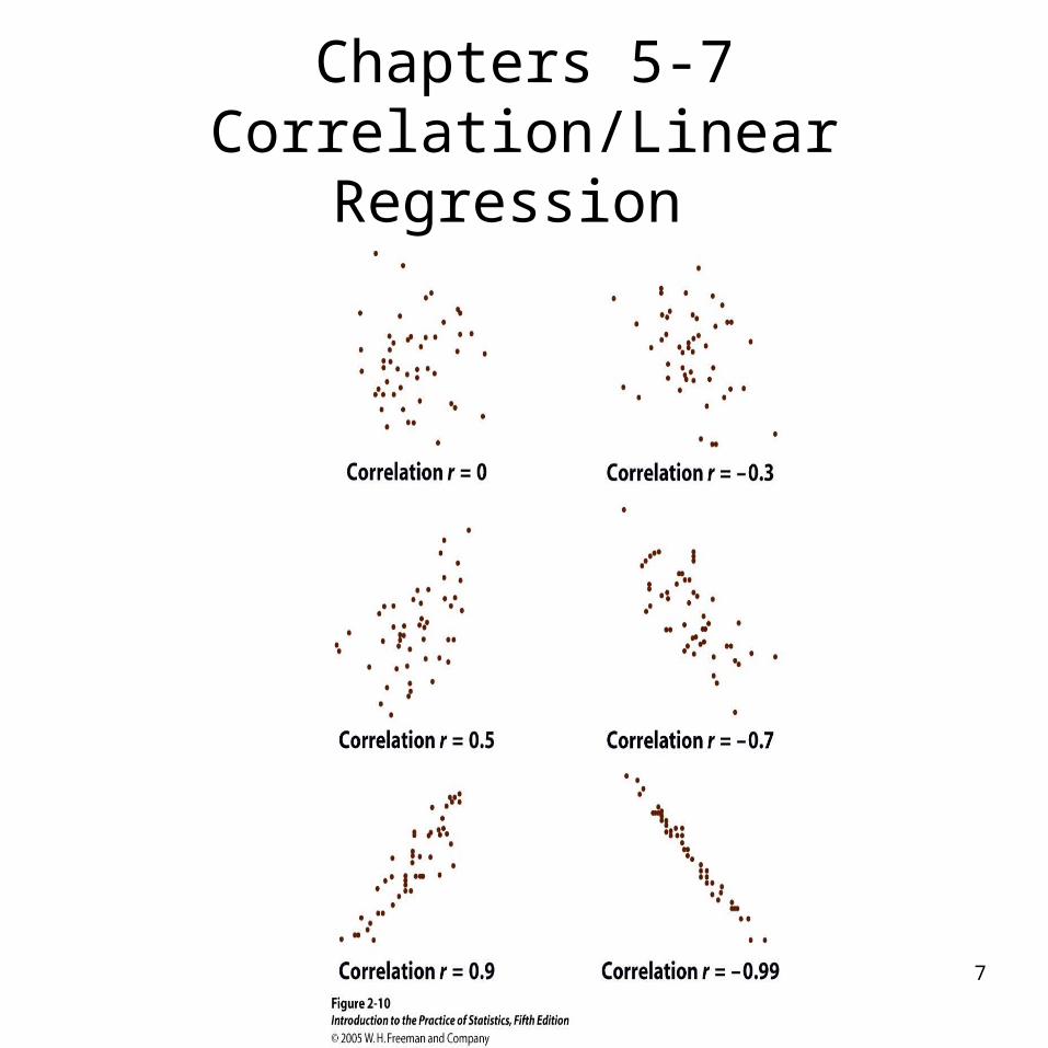
Chapters 5-7 Correlation/Linear Regression
8
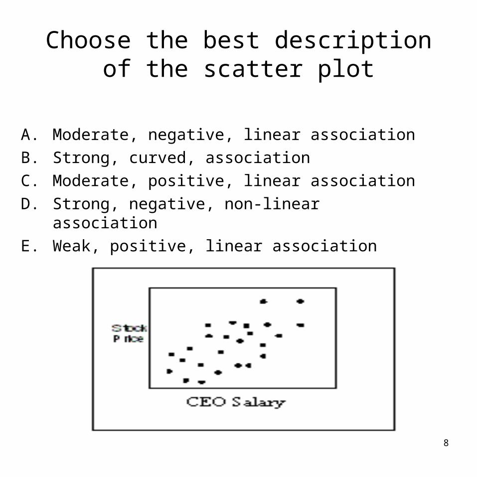
Choose the best description of the scatter plot
A. Moderate, negative, linear association
B. Strong, curved, association
C. Moderate, positive, linear association
D. Strong, negative, non-linear association
E. Weak, positive, linear association
9
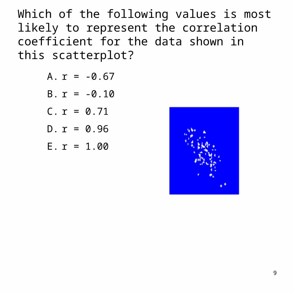
Which of the following values is most likely to represent the correlation coefficient for the data shown in this scatterplot?
A. r = -0.67
B. r = -0.10
C. r = 0.71
D. r = 0.96
E. r = 1.00
10
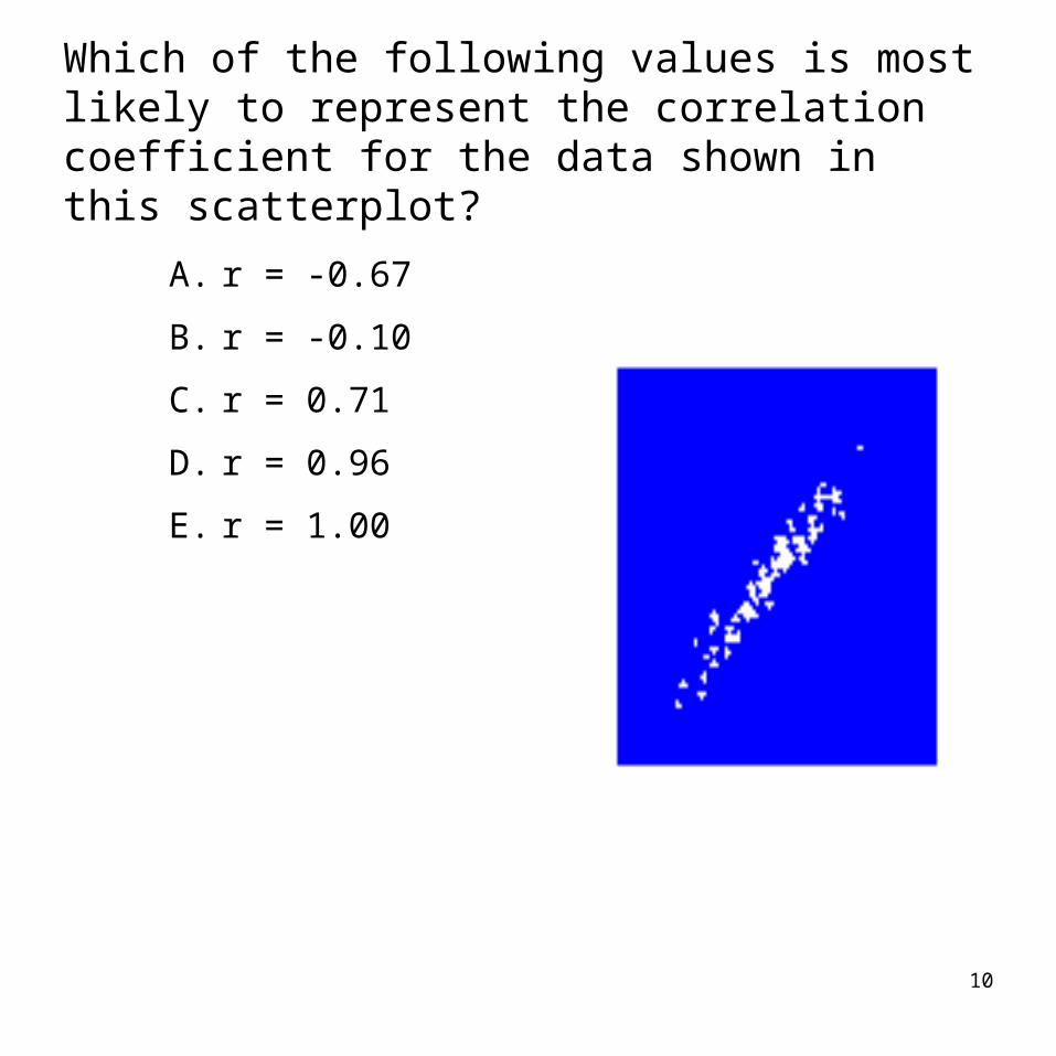
Which of the following values is most likely to represent the correlation coefficient for the data shown in this scatterplot?
A. r = -0.67
B. r = -0.10
C. r = 0.71
D. r = 0.96
E. r = 1.00
11
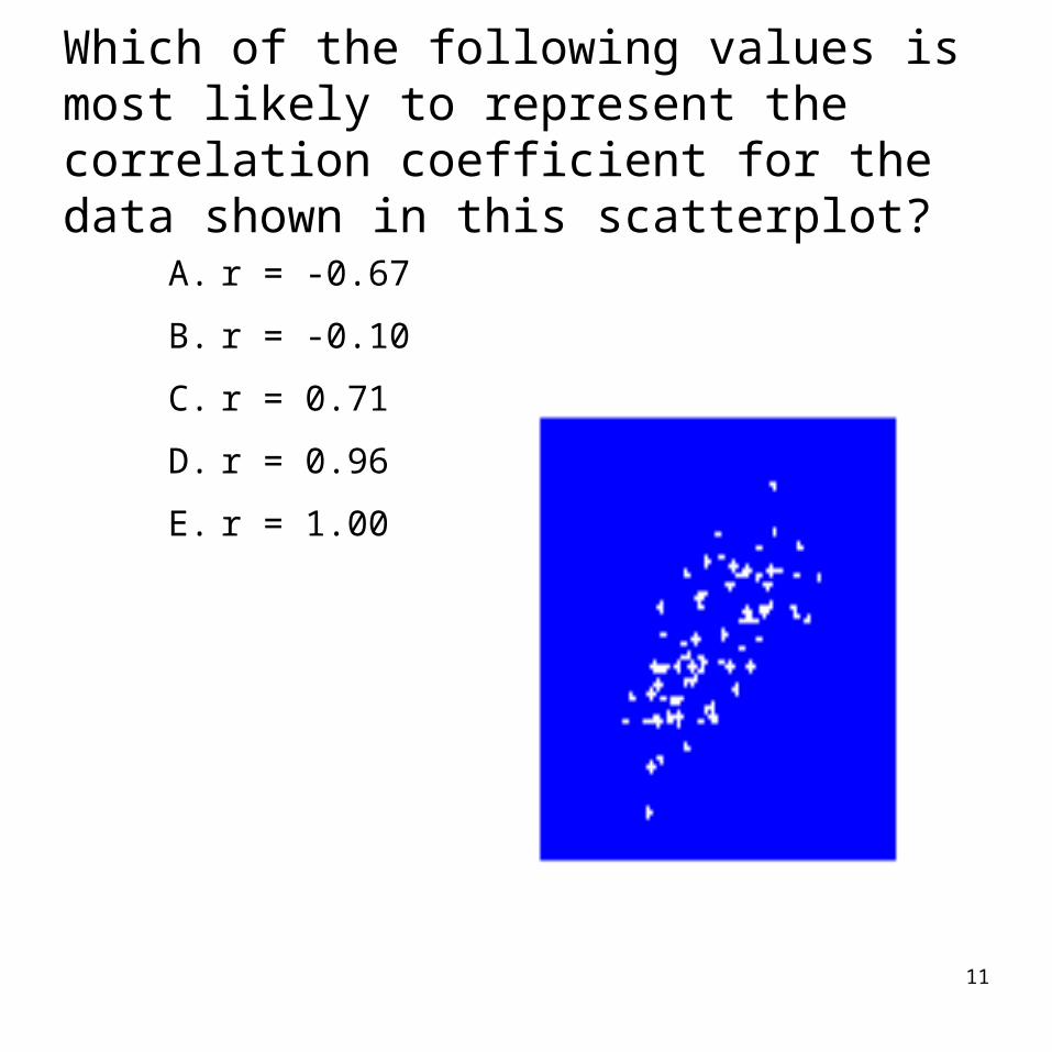
Which of the following values is most likely to represent the correlation coefficient for the data shown in this scatterplot?
A. r = -0.67
B. r = -0.10
C. r = 0.71
D. r = 0.96
E. r = 1.00
12
Cautions about Correlation
• It should only be used– To describe the relationship between 2
QUANTITATIVE variables– When the association is “linear enough”– When there are no outliers
• Correlation does NOT imply causation
13
A teacher at an elementary school measures theheights of children on the playground and then makes ascatter plot of the children’s heights and reading testscores. The data meet the conditions for correlation soshe calculates r = .79. Which conclusion is mostaccurate?
A. Being taller causes students to read betterB. Being shorter causes students to read betterC. Taller students tend to have better reading
scoresD. Shorter students tend to have better reading
scores
14
Chapters 5-7 Correlation/Linear Regression
• Easiest to understand and analyze
• Relationships are often linear
• Variables with non-linear relationship can often be transformed into linear relationship through an appropriate transformation
• Even when a relationship is non-linear, a linear model may provide an accurate approximation for a limited range of values.
• Strength: The strength of a linear relationship is determined by how close the points in the scatterplot lie to a straight line
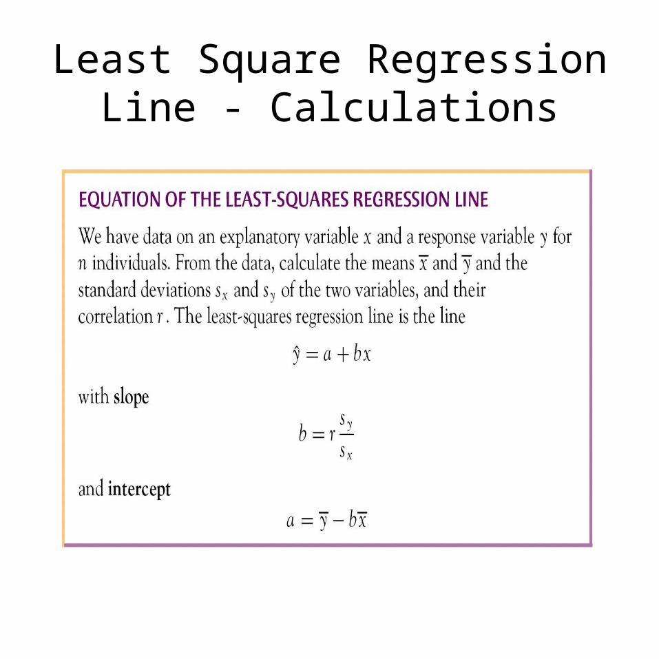
Least Square Regression Line - Calculations
16
Chapters 5-7 Correlation/Linear Regression
• Not all data fall on a straight line!
• Residual = Data – Model or
• Residual = Observed Y – Predicted y
17
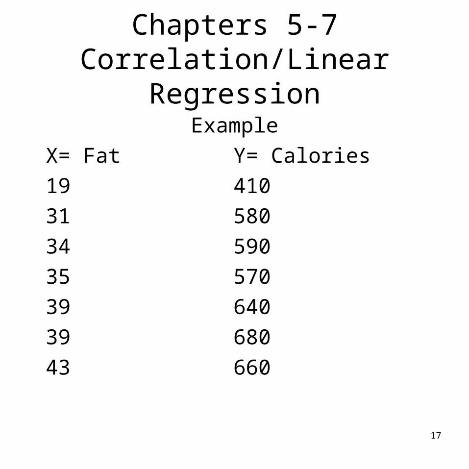
Chapters 5-7 Correlation/Linear Regression
Example
X= Fat Y= Calories
19 410
31 580
34 590
35 570
39 640
39 680
43 660
18
Chapters 5-7 Correlation/Linear Regression
454035302520
700
650
600
550
500
450
400
C1
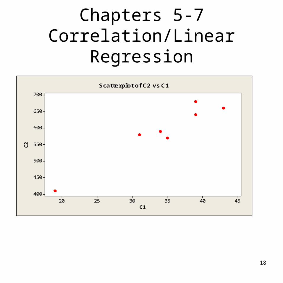
C2
Scatterplot of C2 vs C1
19
Chapters 5-7 Correlation/Linear Regression
454035302520
700
650
600
550
500
450
400
C1
C2
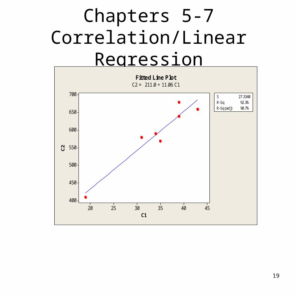
S 27.3340R-Sq 92.3%R-Sq(adj) 90.7%
Fitted Line PlotC2 = 211.0 + 11.06 C1
20
Chapters 5-7 Correlation/Linear Regression
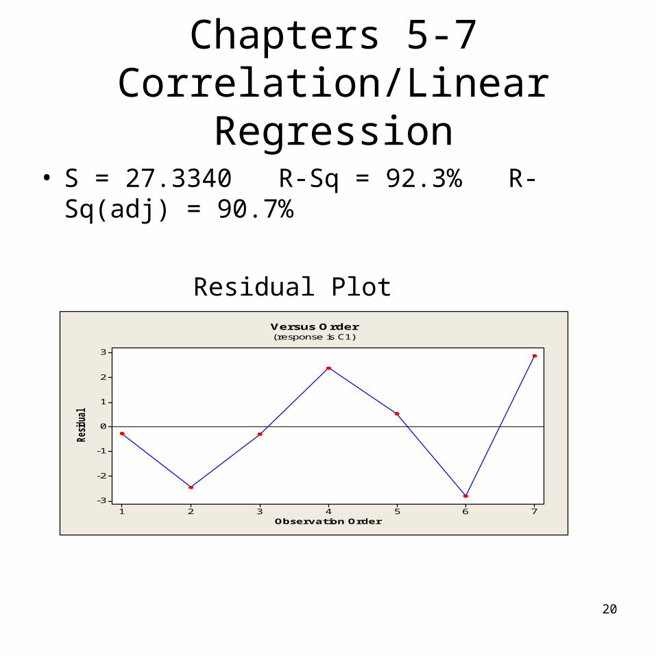
• S = 27.3340 R-Sq = 92.3% R-Sq(adj) = 90.7%
Residual Plot
7654321
3
2
1
0
-1
-2
-3
Observation Order
Residual
Versus Order(response is C1)

21
Chapters 5-7 Correlation/Linear Regression
• Extrapolation: Reaching beyond the data
• Outliers: Regression models are sensitive to outliers
• Leverage: An unusual data point whose x value is far from the mean of the x values
• A point with high leverage has the potential to change the regression line.
22
Chapters 5-7 Correlation/Linear Regression
• Influential: A point is influential if omitting it from the analysis gives a very different model.
• Influence depends on leverage and residual
• Lurking variables: A variable that is not included in the construction of the linear model/study.
23
Chapters 5-7 Correlation/Linear Regression
• Lurking variables may influence correlation and regression models.
• Association is not causations!!
24
Summary
• r is a number between -1 and 1• r = 1 or r = -1 indicates a perfect
correlation case where all data points lie on a straight line
• r > 0 indicates positive association• r < 0 indicates negative association• r value does not change when units of
measurement are changed (correlation has no units!)
• Correlation treats X and Y symmetrically. The correlation of X with Y is the same as the correlation of Y with X
25
Summary
• Quantitative variable condition: Do not apply correlation to categorical variables
• Correlation can be misleading if the relationship is not linear
• Outliers distort correlation dramatically. Report correlation with/without outliers.
26
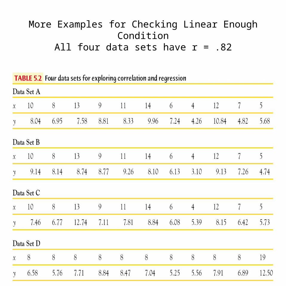
More Examples for Checking Linear Enough ConditionAll four data sets have r = .82
27
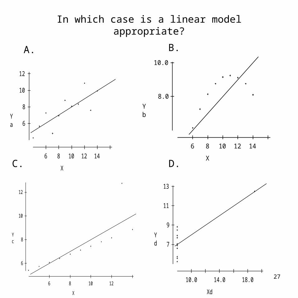
In which case is a linear model appropriate?
6
8
10
12
6 8 10 12 14
X
Ya
8.0
10.0
6 8 10 12 14
X
Yb
6
8
10
12
6 8 10 12
X
Yc 7
9
11
13
10.0 14.0 18.0
Xd
Yd
A. B.
C. D.
28
6
8
10
12
6 8 10 12 14
X
Ya -1
0
1
6 8 10 12 14
X
residuals(Y/X)
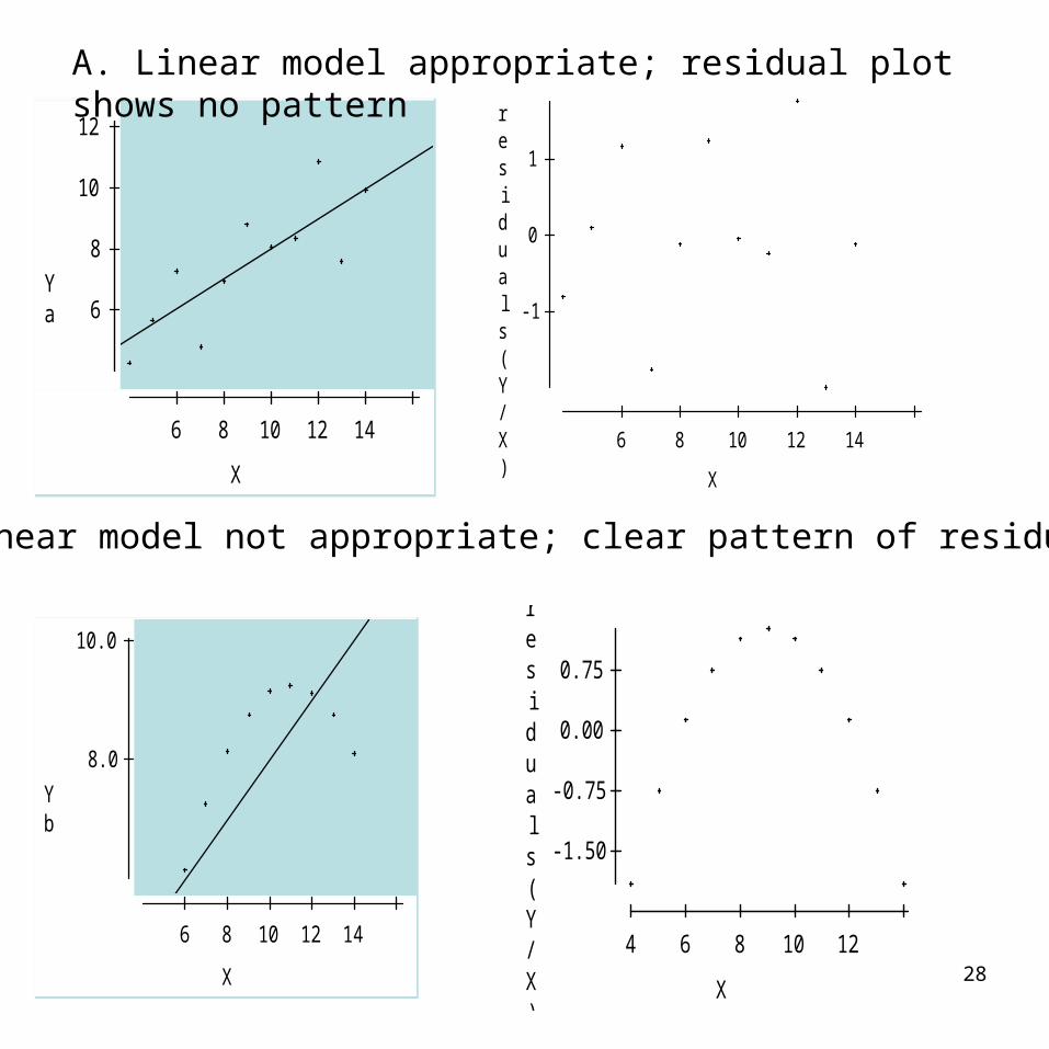
A. Linear model appropriate; residual plot shows no pattern
8.0
10.0
6 8 10 12 14
X
Yb
-1.50
-0.75
0.00
0.75
4 6 8 10 12
X
residuals(Y/X)
B. Linear model not appropriate; clear pattern of residuals
29
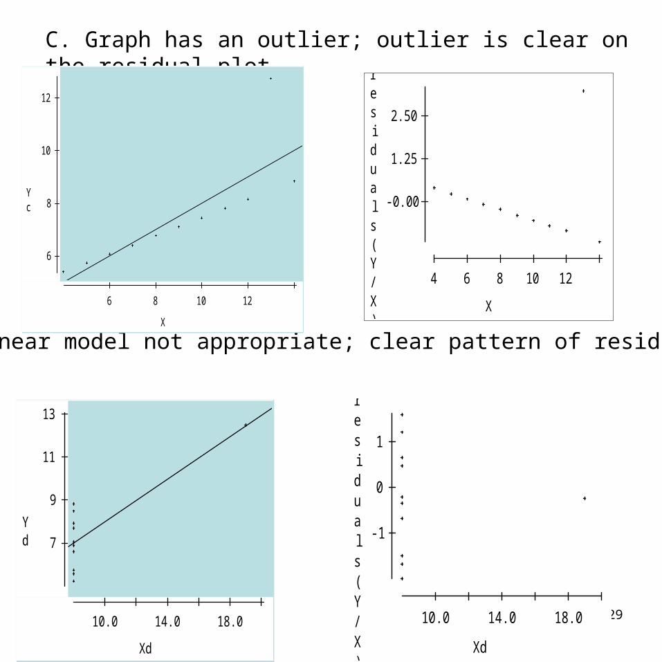
C. Graph has an outlier; outlier is clear on the residual plot
D. Linear model not appropriate; clear pattern of residuals
6
8
10
12
6 8 10 12
X
Yc -0.00
1.25
2.50
4 6 8 10 12
X
residuals(Y/X)
7
9
11
13
10.0 14.0 18.0
Xd
Yd -1
0
1
10.0 14.0 18.0
Xd
residuals(Y/X)
30
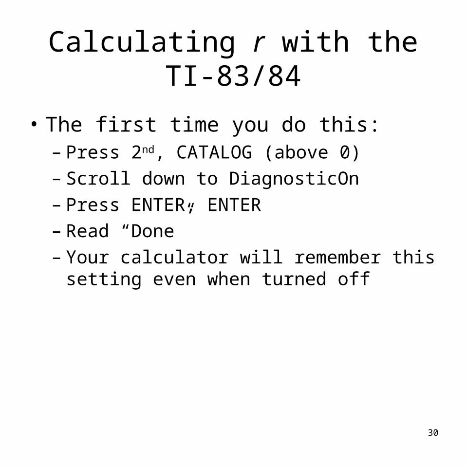
Calculating r with the TI-83/84
• The first time you do this:– Press 2nd, CATALOG (above 0)– Scroll down to DiagnosticOn– Press ENTER, ENTER– Read “Done”– Your calculator will remember this setting
even when turned off
31
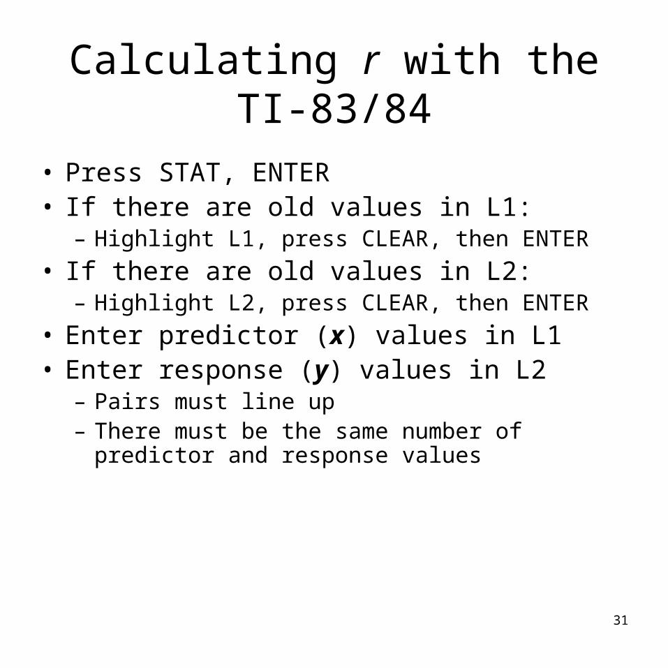
Calculating r with the TI-83/84
• Press STAT, ENTER• If there are old values in L1:
– Highlight L1, press CLEAR, then ENTER
• If there are old values in L2:– Highlight L2, press CLEAR, then ENTER
• Enter predictor (x) values in L1• Enter response (y) values in L2
– Pairs must line up– There must be the same number of predictor and
response values
32
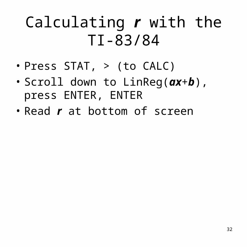
Calculating r with the TI-83/84
• Press STAT, > (to CALC)
• Scroll down to LinReg(ax+b), press ENTER, ENTER
• Read r at bottom of screen
33
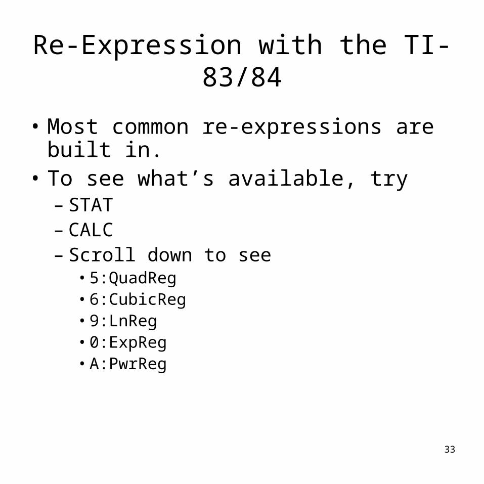
Re-Expression with the TI-83/84
• Most common re-expressions are built in.• To see what’s available, try
– STAT– CALC– Scroll down to see
• 5:QuadReg• 6:CubicReg• 9:LnReg• 0:ExpReg• A:PwrReg
34
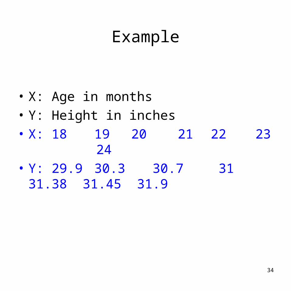
Example
• X: Age in months
• Y: Height in inches
• X: 18 19 20 21 22 23 24
• Y: 29.9 30.3 30.7 31 31.38 31.45 31.9
35
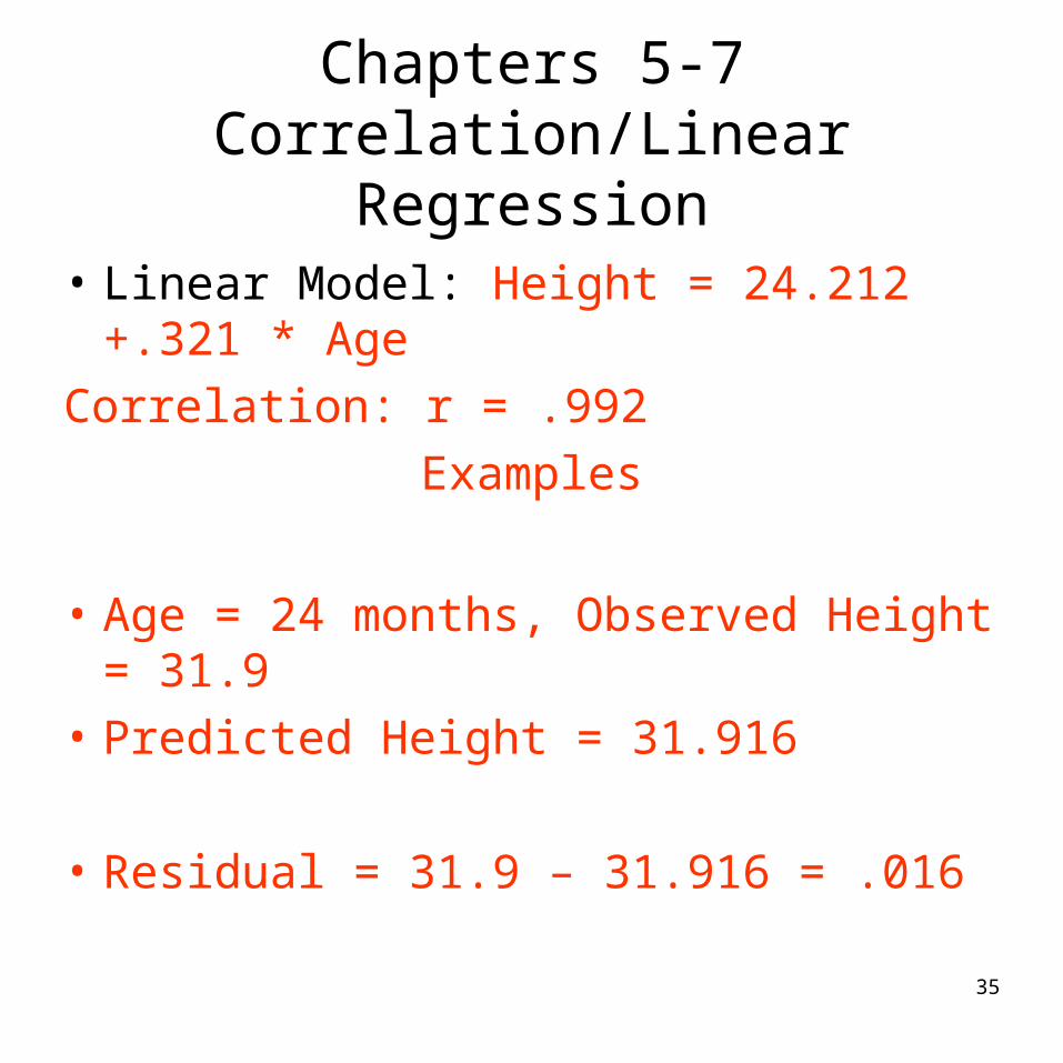
Chapters 5-7 Correlation/Linear Regression
• Linear Model: Height = 24.212 +.321 * Age
Correlation: r = .992
Examples
• Age = 24 months, Observed Height = 31.9
• Predicted Height = 31.916
• Residual = 31.9 – 31.916 = .016
36
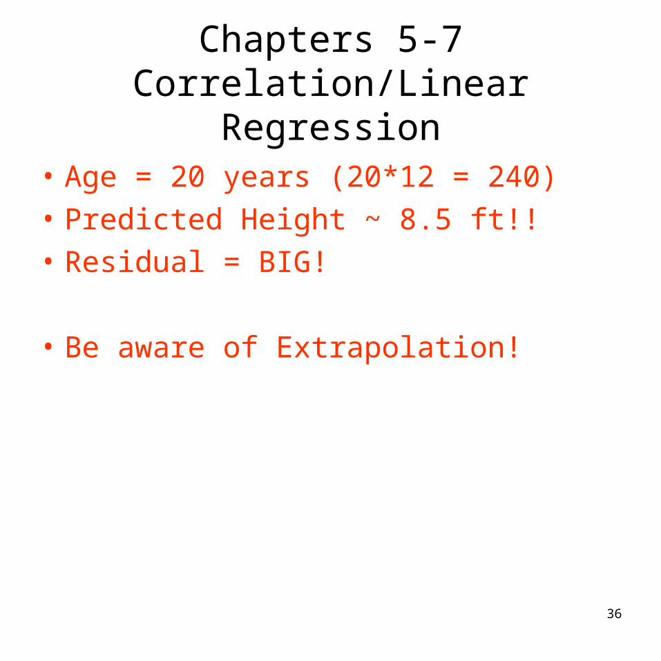
Chapters 5-7 Correlation/Linear Regression
• Age = 20 years (20*12 = 240)
• Predicted Height ~ 8.5 ft!!
• Residual = BIG!
• Be aware of Extrapolation!
37
Example
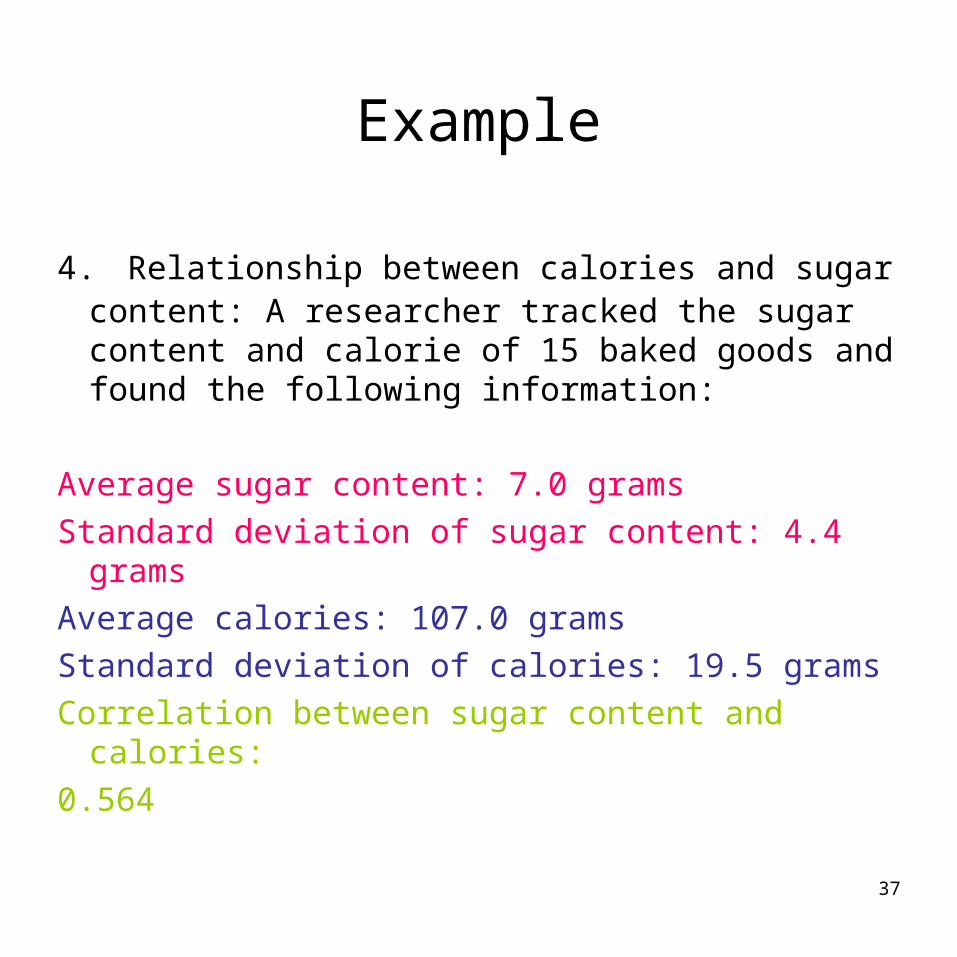
4. Relationship between calories and sugar content: A researcher tracked the sugar content and calorie of 15 baked goods and found the following information:
Average sugar content: 7.0 grams
Standard deviation of sugar content: 4.4 grams
Average calories: 107.0 grams
Standard deviation of calories: 19.5 grams
Correlation between sugar content and calories:
0.564
38
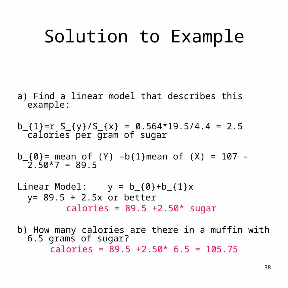
Solution to Example
a) Find a linear model that describes this example:
b_{1}=r S_{y}/S_{x} = 0.564*19.5/4.4 = 2.5 calories per gram of sugar
b_{0}= mean of (Y) –b{1}mean of (X) = 107 -2.50*7 = 89.5
Linear Model: y = b_{0}+b_{1}x y= 89.5 + 2.5x or better
calories = 89.5 +2.50* sugar
b) How many calories are there in a muffin with 6.5 grams of sugar?
calories = 89.5 +2.50* 6.5 = 105.75
39
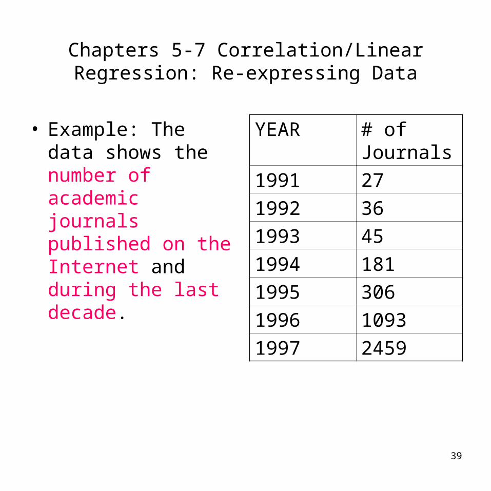
Chapters 5-7 Correlation/Linear Regression: Re-expressing Data
• Example: The data shows the number of academic journals published on the Internet and during the last decade.
YEAR # of Journals
1991 27
1992 36
1993 45
1994 181
1995 306
1996 1093
1997 2459
40
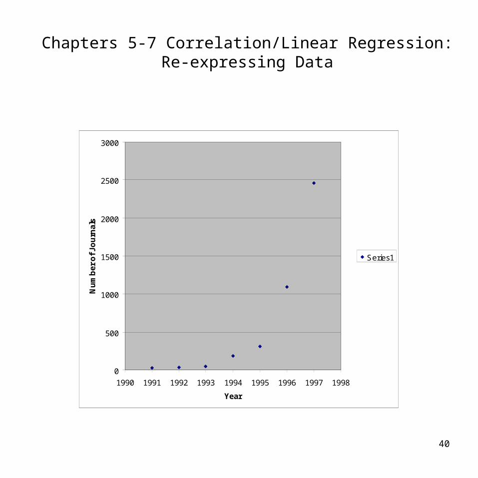
Chapters 5-7 Correlation/Linear Regression: Re-expressing Data
0
500
1000
1500
2000
2500
3000
1990 1991 1992 1993 1994 1995 1996 1997 1998
Year
Nu
mb
er
of
Jo
urn
als
Series1
41
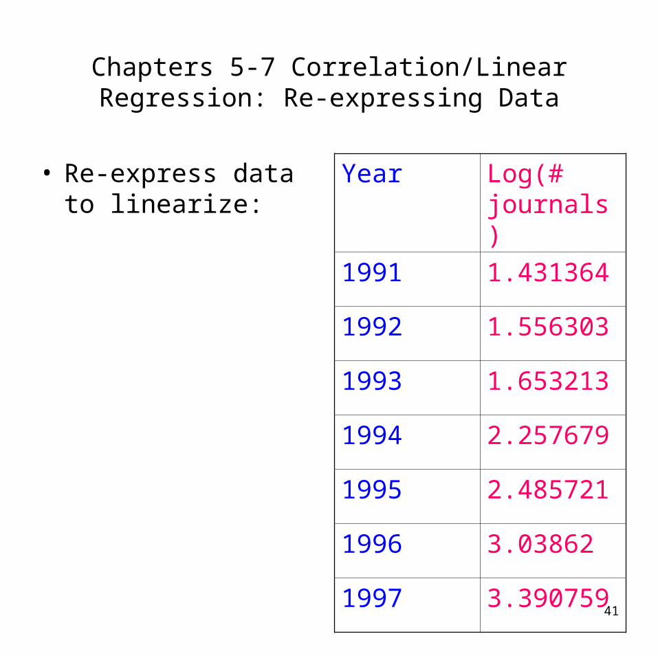
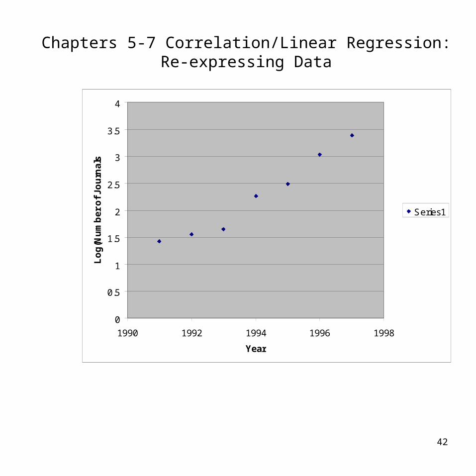
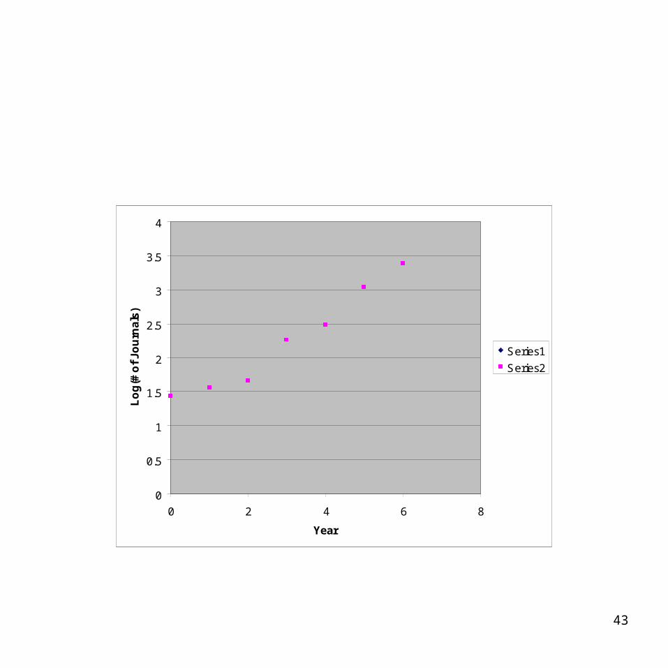
Chapters 5-7 Correlation/Linear Regression: Re-expressing Data
• Re-express data to linearize:
Year Log(# journals)
1991 1.431364
1992 1.556303
1993 1.653213
1994 2.257679
1995 2.485721
1996 3.03862
1997 3.390759
42
Chapters 5-7 Correlation/Linear Regression: Re-expressing Data
0
0.5
1
1.5
2
2.5
3
3.5
4
1990 1992 1994 1996 1998
Year
Lo
g(N
um
be
r o
f J
ou
rna
ls
Series1
43
0
0.5
1
1.5
2
2.5
3
3.5
4
0 2 4 6 8
Year
Lo
g(#
of
Jo
urn
als
)
Series1
Series2
44
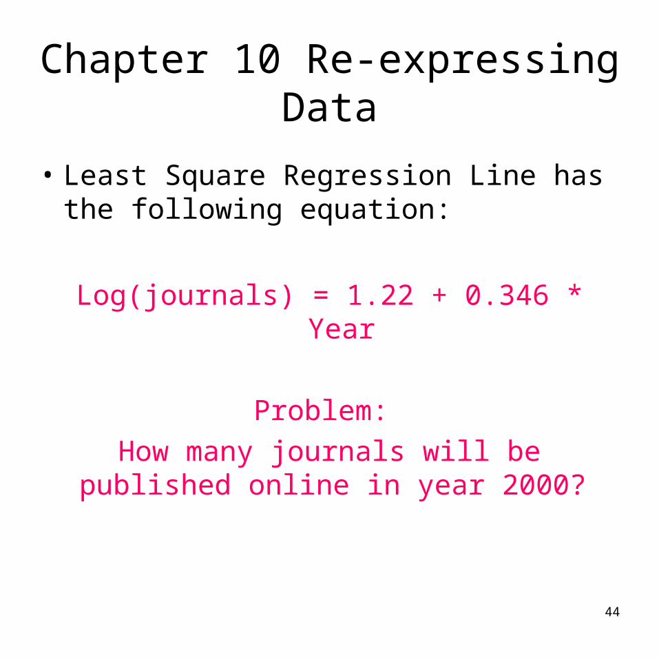
Chapter 10 Re-expressing Data
• Least Square Regression Line has the following equation:
Log(journals) = 1.22 + 0.346 * Year
Problem:
How many journals will be published online in year 2000?
45
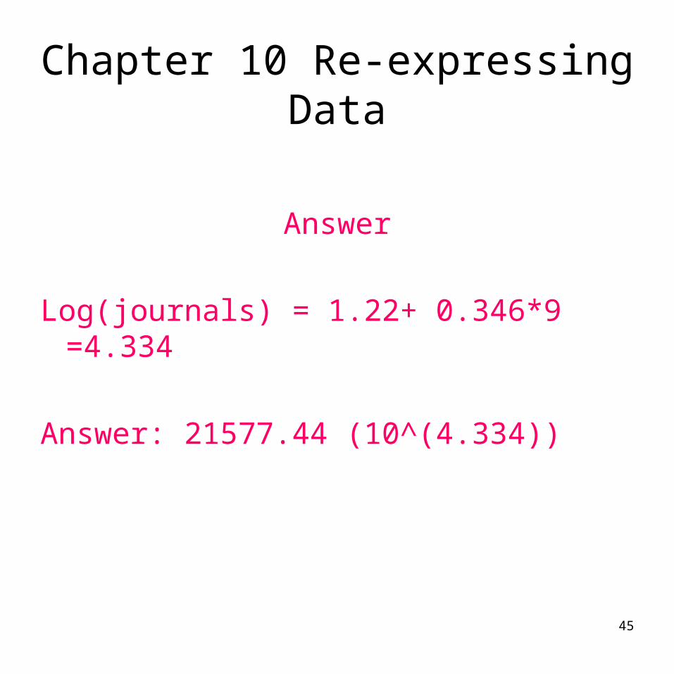
Chapter 10 Re-expressing Data
Answer
Log(journals) = 1.22+ 0.346*9 =4.334
Answer: 21577.44 (10^(4.334))
46
Chapter 10 Re-expressing Data
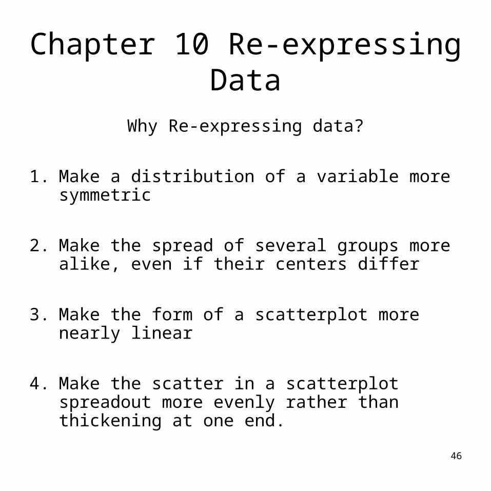
Why Re-expressing data?
1. Make a distribution of a variable more symmetric
2. Make the spread of several groups more alike, even if their centers differ
3. Make the form of a scatterplot more nearly linear
4. Make the scatter in a scatterplot spreadout more evenly rather than thickening at one end.
47
Chapter 10 Re-expressing Data
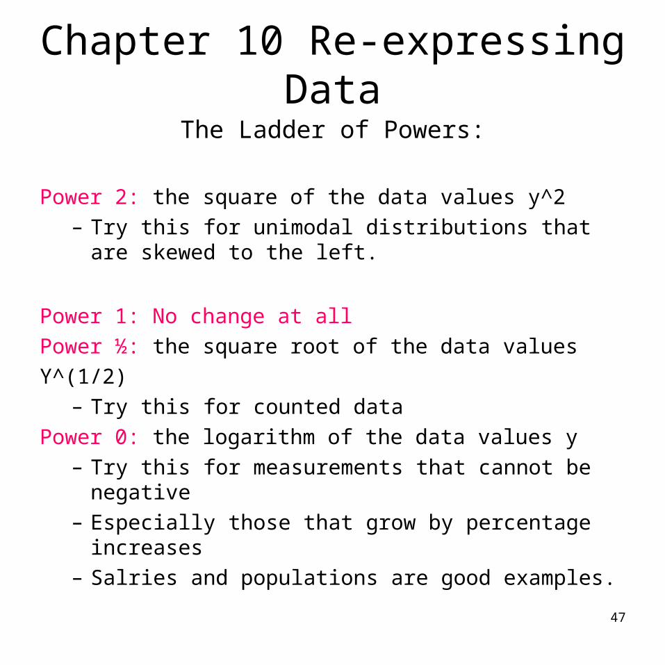
The Ladder of Powers:
Power 2: the square of the data values y^2– Try this for unimodal distributions that are skewed to
the left.
Power 1: No change at all
Power ½: the square root of the data values
Y^(1/2)– Try this for counted data
Power 0: the logarithm of the data values y– Try this for measurements that cannot be negative– Especially those that grow by percentage increases– Salries and populations are good examples.