Chapters 13-15

Net value and marginal analysis• Decision rules• Example

Present value analysis• Reconciling present and future cash flows• Discounting

Figures of merit• Weighted sum• Delivered system capability

Multiple Goal Decision Analysis I

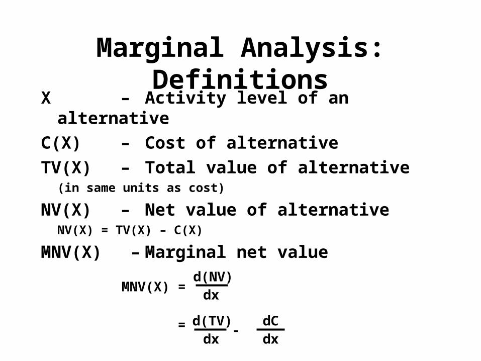
Marginal Analysis: DefinitionsX – Activity level of an alternative

C(X) – Cost of alternative

TV(X) – Total value of alternative (in same units as cost)

NV(X) – Net value of alternativeNV(X) = TV(X) – C(X)

MNV(X) – Marginal net value

MNV(X) =

= -dx

d(NV)

dC

dx

d(TV)dx

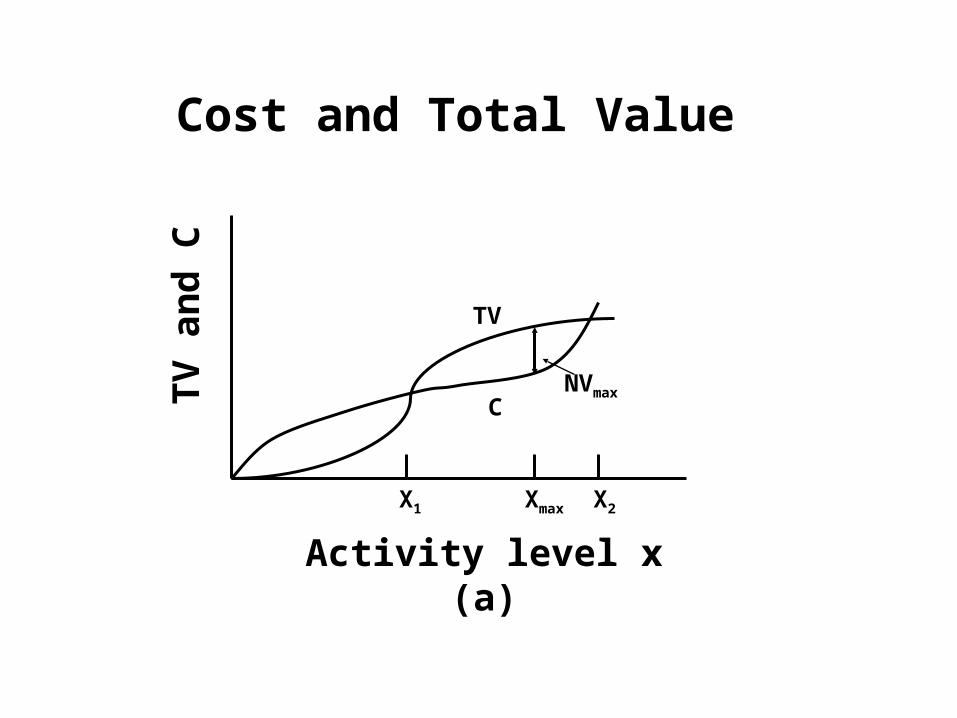
CNVmax

Xmax X2

Activity level x(a)

TV

an

d C

Cost and Total Value

TV

X1

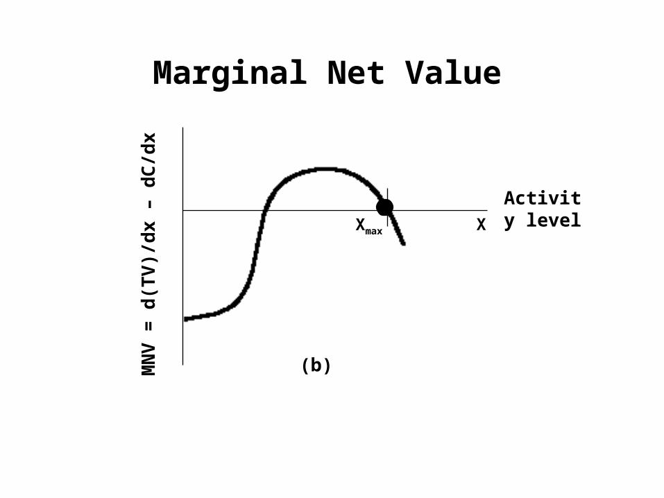
(b)

MN

V =

d(T

V)/

dx

– d

C/d

x

Marginal Net Value

Xmax X

Activity level

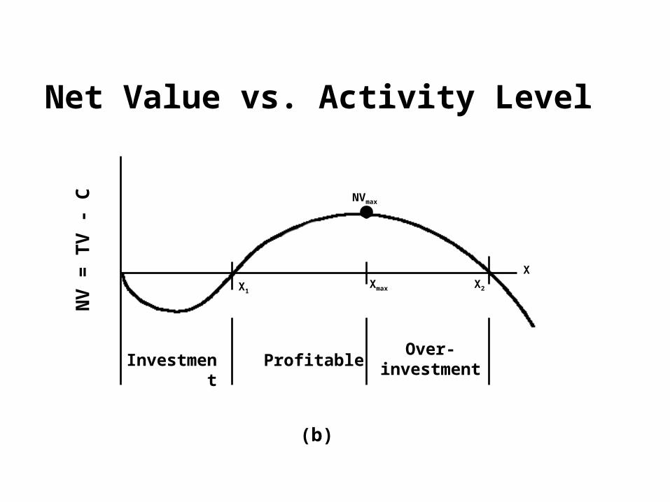
X1Xmax X2

Over-investment

(b)

NV

= T

V -

C

X

NVmax

Net Value vs. Activity Level

Investment Profitable

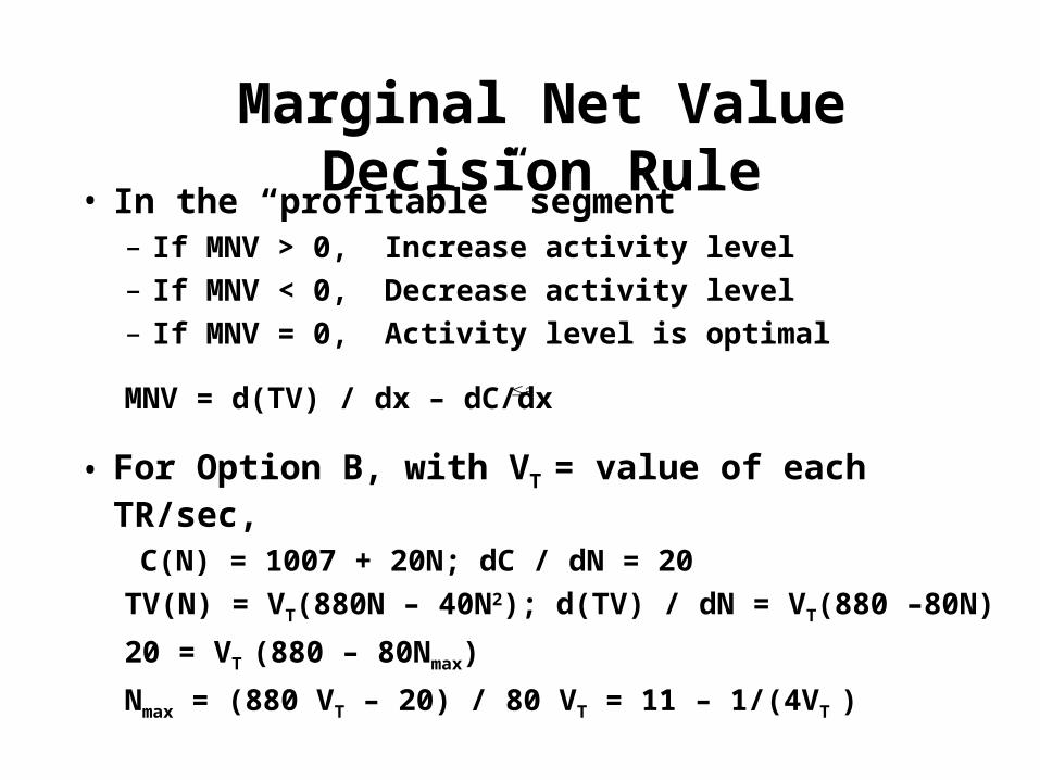
Marginal Net Value Decision Rule• In the “profitable” segment

– If MNV > 0, Increase activity level– If MNV < 0, Decrease activity level– If MNV = 0, Activity level is optimal

MNV = d(TV) / dx – dC/dx

• For Option B, with VT = value of each TR/sec,

C(N) = 1007 + 20N; dC / dN = 20

TV(N) = VT(880N – 40N2); d(TV) / dN = VT(880 –80N)

20 = VT (880 – 80Nmax)

Nmax = (880 VT – 20) / 80 VT = 11 – 1/(4VT )

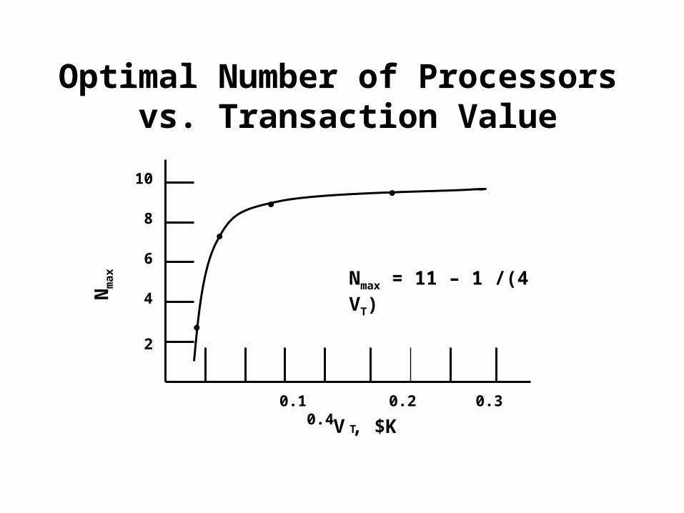
Optimal Number of Processors vs. Transaction Value

0.1 0.2 0.3 0.4

2

4

6

8

10

Nm

ax

V T, $K

Nmax = 11 – 1 /(4 VT)

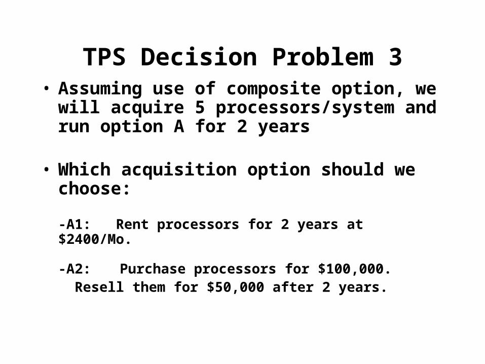
TPS Decision Problem 3• Assuming use of composite option, we

will acquire 5 processors/system and run option A for 2 years

• Which acquisition option should we choose:

-A1: Rent processors for 2 years at $2400/Mo.

-A2: Purchase processors for $100,000. Resell them for $50,000 after 2 years.

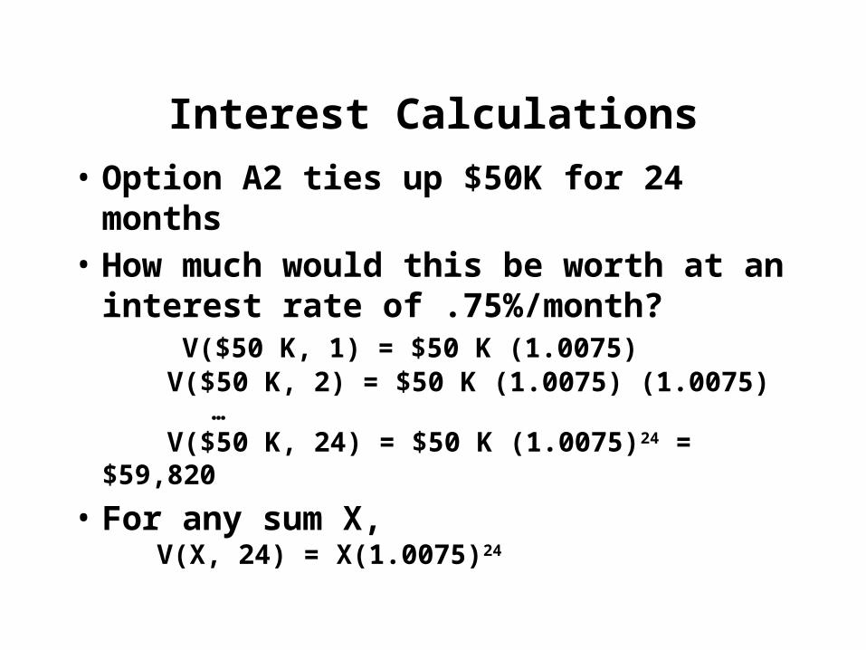
Interest Calculations

• Option A2 ties up $50K for 24 months• How much would this be worth at an

interest rate of .75%/month? V($50 K, 1) = $50 K (1.0075) V($50 K, 2) = $50 K (1.0075) (1.0075) … V($50 K, 24) = $50 K (1.0075)24 = $59,820

• For any sum X, V(X, 24) = X(1.0075)24

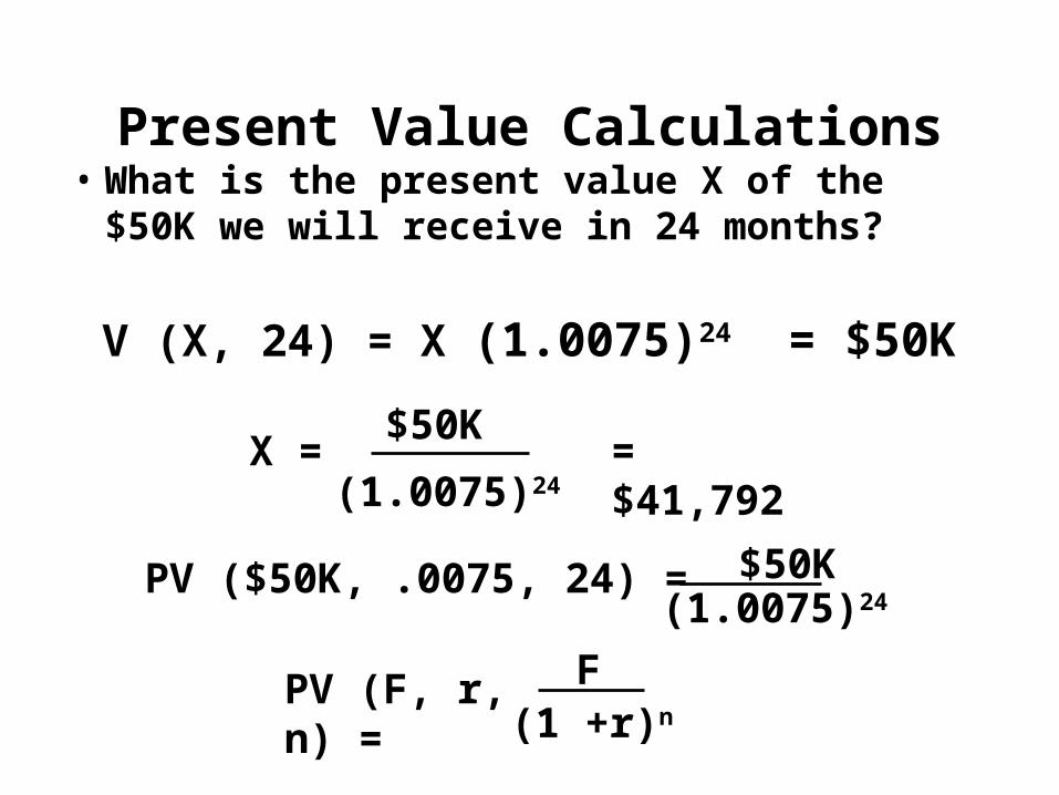
Present Value Calculations• What is the present value X of the

$50K we will receive in 24 months?

X = = $41,792

$50K

PV (F, r, n) =

(1.0075)24

$50K

V (X, 24) = X (1.0075)24 = $50K

PV ($50K, .0075, 24) =

F(1 +r)n

(1.0075)24

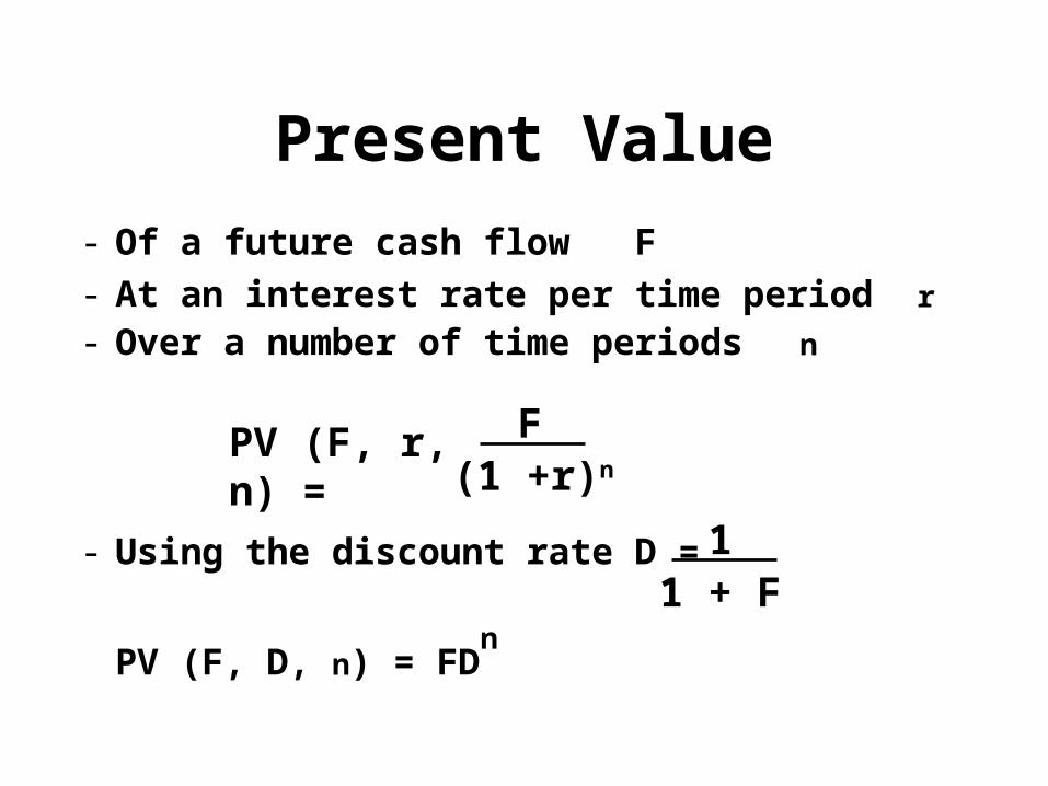
- Of a future cash flow F- At an interest rate per time period r- Over a number of time periods n

- Using the discount rate D =

PV (F, D, n) = FDn

Present Value

PV (F, r, n) = F(1 +r)n

11 + F

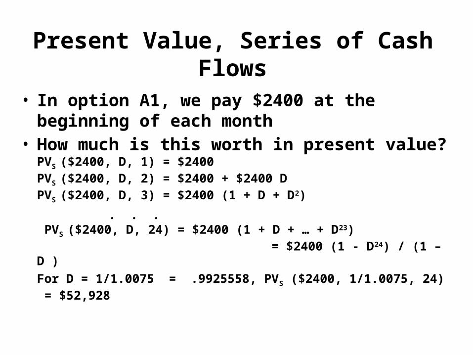
Present Value, Series of Cash Flows

• In option A1, we pay $2400 at the beginning of each month

• How much is this worth in present value?PVS ($2400, D, 1) = $2400PVS ($2400, D, 2) = $2400 + $2400 DPVS ($2400, D, 3) = $2400 (1 + D + D2)

. . . PVS ($2400, D, 24) = $2400 (1 + D + … + D23) = $2400 (1 - D24) / (1 – D )

For D = 1/1.0075 = .9925558, PVS ($2400, 1/1.0075, 24) = $52,928

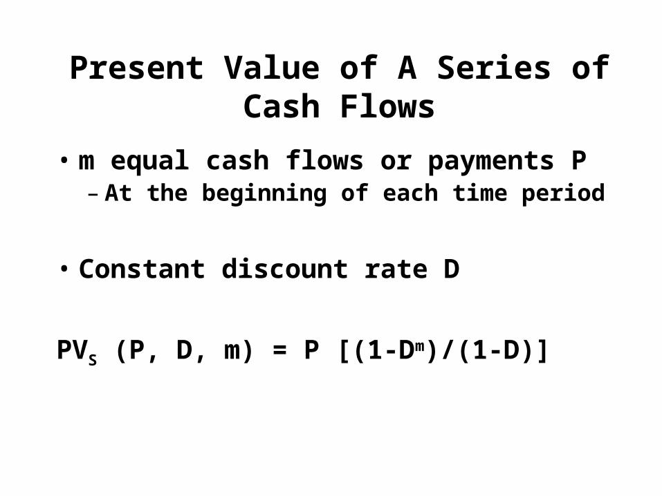
Present Value of A Series of Cash Flows

• m equal cash flows or payments P– At the beginning of each time period

• Constant discount rate D

PVS (P, D, m) = P [(1-Dm)/(1-D)]

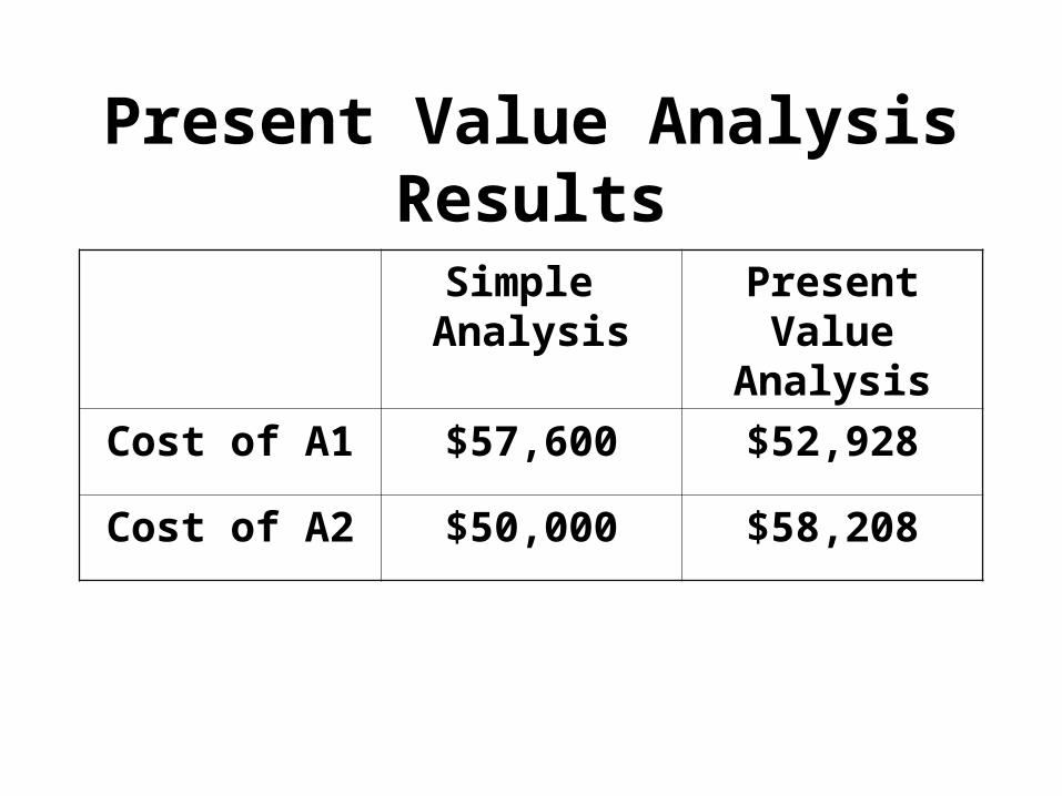
Present Value Analysis Results

Simple Analysis

Present Value Analysis

Cost of A1 $57,600 $52,928

Cost of A2 $50,000 $58,208

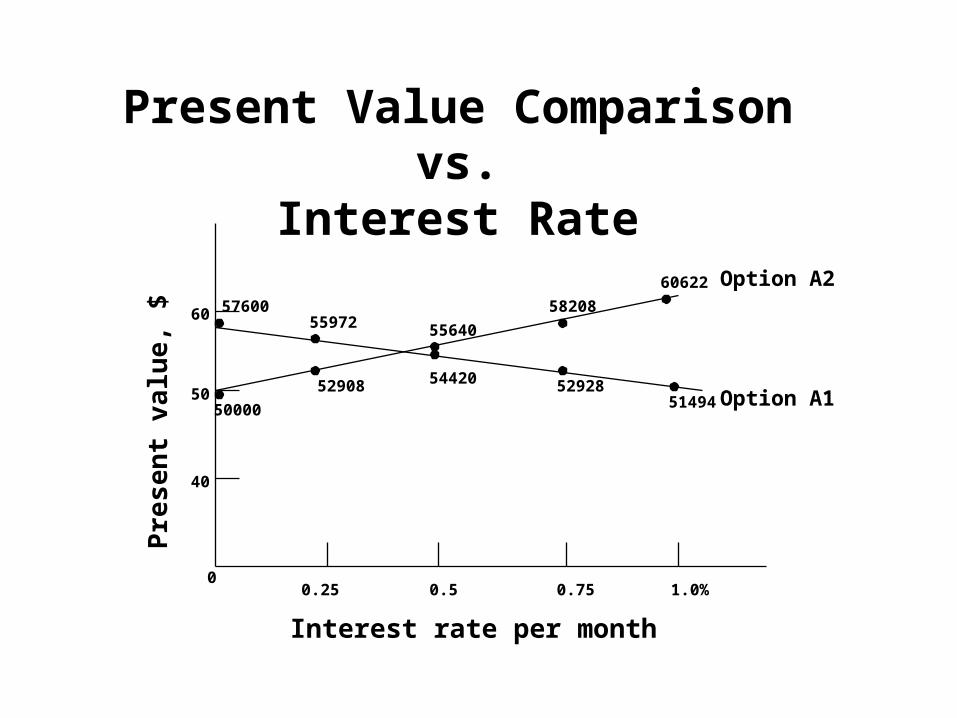
5760055972 55640

58208

60622

50000

52908 54420 5292851494

60

50

40

00.25 0.5 0.75 1.0%

Interest rate per month

Pre

sen

t va

lue,

$

Present Value Comparisonvs.

Interest RateOption A2

Option A1

TPS Decision Problem 4• Choose best vendor operating system

– System A – Standard OS

– System A Plus• Better diagnostics, maintenance features• $40K added cost

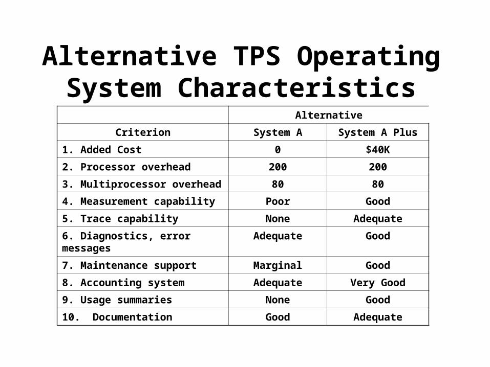
Alternative TPS Operating System Characteristics

Alternative

Criterion System A System A Plus

1. Added Cost 0 $40K

2. Processor overhead 200 200

3. Multiprocessor overhead 80 80

4. Measurement capability Poor Good

5. Trace capability None Adequate

6. Diagnostics, error messages Adequate Good

7. Maintenance support Marginal Good

8. Accounting system Adequate Very Good

9. Usage summaries None Good

10. Documentation Good Adequate

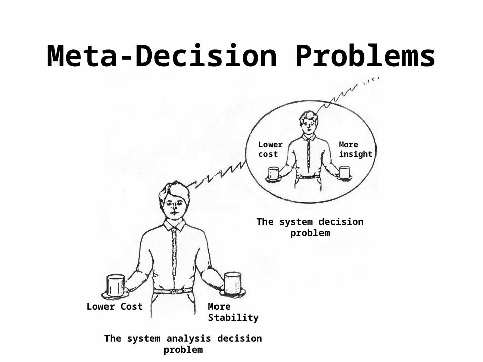
Meta-Decision Problems

Lower Cost More Stability

Lowercost

More insight

The system decision problem

The system analysis decision problem

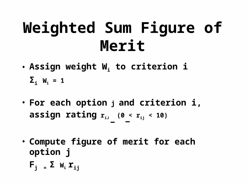
Weighted Sum Figure of Merit

• Assign weight Wi to criterion i

Σi Wi = 1

• For each option j and criterion i, assign rating riJ (0 < rij < 10)

• Compute figure of merit for each option j

Fj = Σ Wi rij

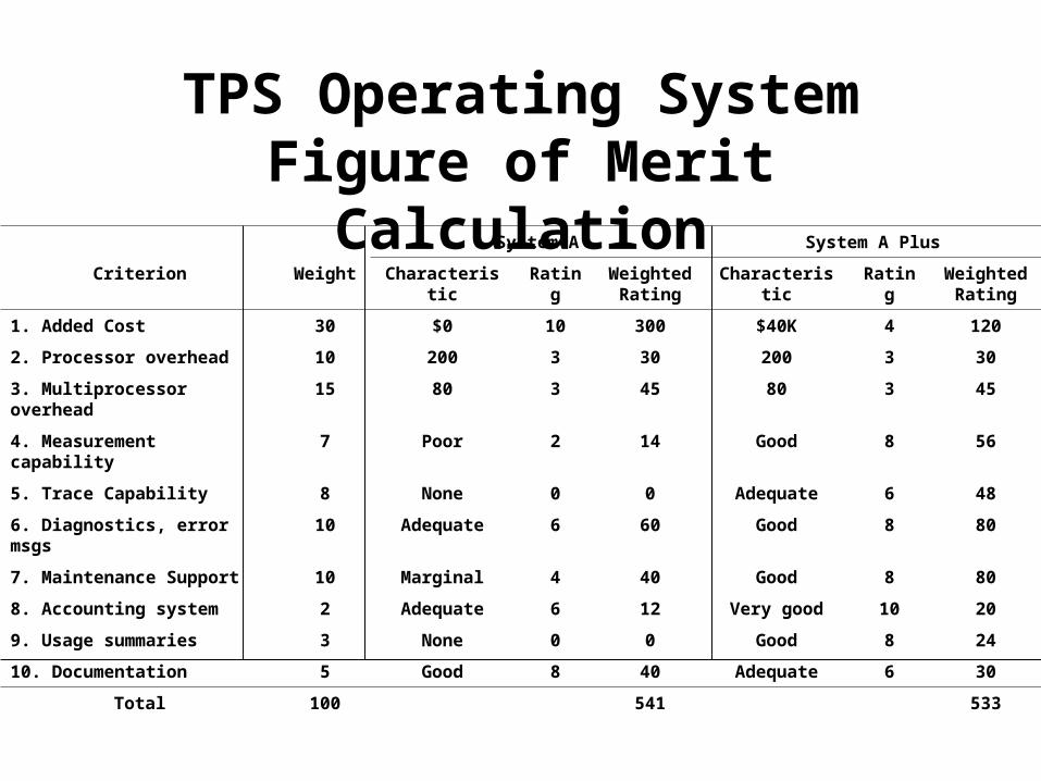
TPS Operating System Figure of Merit Calculation

System A System A Plus

Criterion Weight Characteristic Rating Weighted Rating

Characteristic Rating Weighted Rating

1. Added Cost 30 $0 10 300 $40K 4 120

2. Processor overhead 10 200 3 30 200 3 30

3. Multiprocessor overhead 15 80 3 45 80 3 45

4. Measurement capability 7 Poor 2 14 Good 8 56

5. Trace Capability 8 None 0 0 Adequate 6 48

6. Diagnostics, error msgs 10 Adequate 6 60 Good 8 80

7. Maintenance Support 10 Marginal 4 40 Good 8 80

8. Accounting system 2 Adequate 6 12 Very good 10 20

9. Usage summaries 3 None 0 0 Good 8 24

10. Documentation 5 Good 8 40 Adequate 6 30

Total 100 541 533

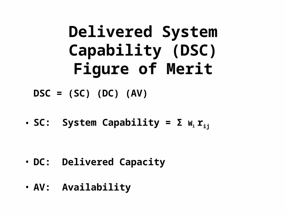
Delivered System Capability (DSC)

Figure of Merit

DSC = (SC) (DC) (AV)

• SC: System Capability = Σ Wi rij

• DC: Delivered Capacity

• AV: Availability

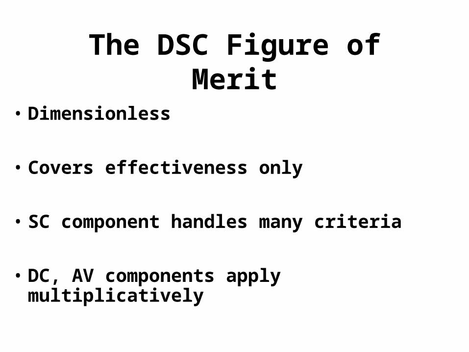
The DSC Figure of Merit

• Dimensionless

• Covers effectiveness only

• SC component handles many criteria

• DC, AV components apply multiplicatively

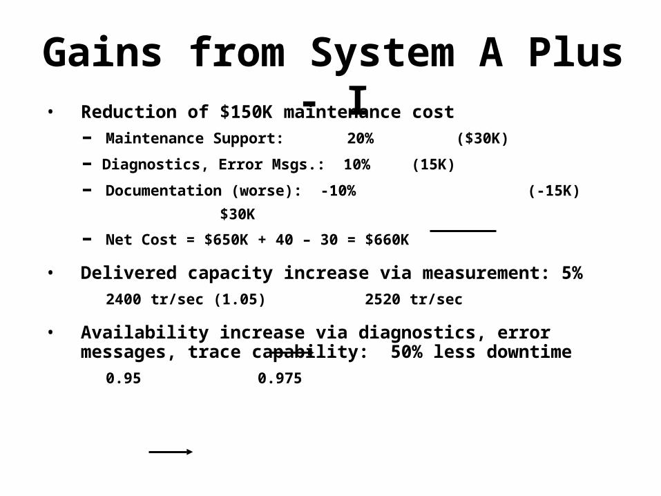
• Reduction of $150K maintenance cost

– Maintenance Support: 20% ($30K)

– Diagnostics, Error Msgs.: 10% (15K)

– Documentation (worse): -10% (-15K)

$30K

– Net Cost = $650K + 40 – 30 = $660K

• Delivered capacity increase via measurement: 5%

2400 tr/sec (1.05) 2520 tr/sec

• Availability increase via diagnostics, error messages, trace capability: 50% less downtime

0.95 0.975

Gains from System A Plus - I

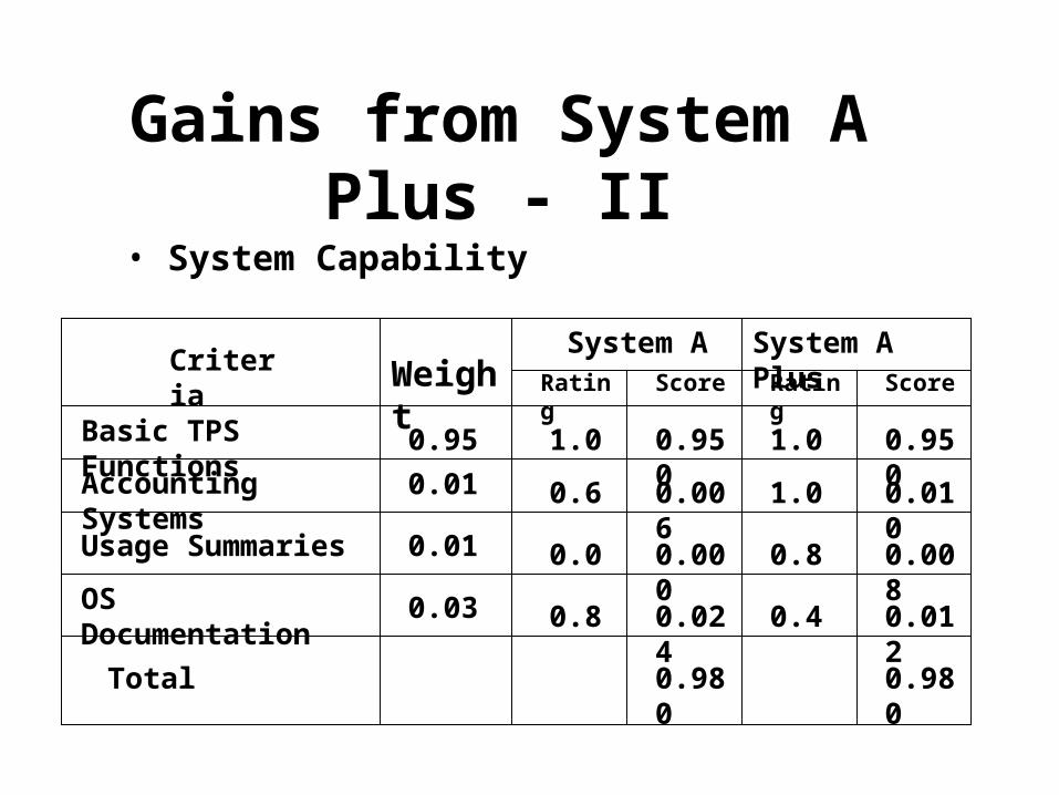
Gains from System A Plus - II• System Capability

WeightSystem A

Rating Score

System A PlusRating Score

Criteria

Total

Basic TPS Functions

Accounting Systems

Usage Summaries

OS Documentation

0.95

0.01

0.01

0.03

1.0

0.6

0.0

0.8

0.950

0.006

0.000

0.024

1.0

1.0

0.8

0.4

0.950

0.010

0.008

0.012

0.980 0.980

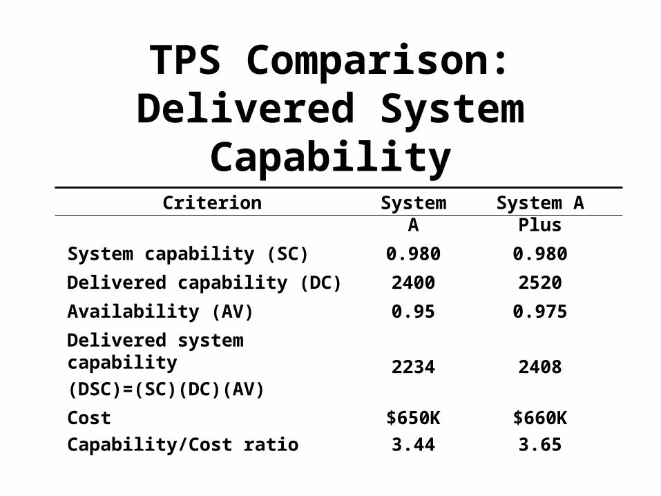
TPS Comparison: Delivered System Capability

Criterion System A System A Plus

System capability (SC) 0.980 0.980

Delivered capability (DC) 2400 2520

Availability (AV) 0.95 0.975

Delivered system capability

(DSC)=(SC)(DC)(AV) 2234 2408

Cost

Capability/Cost ratio

$650K

3.44

$660K

3.65

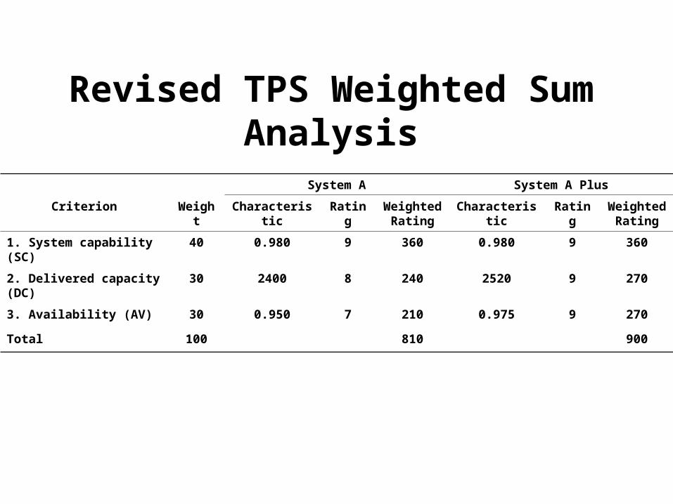
Revised TPS Weighted Sum Analysis

System A System A Plus

Criterion Weight Characteristic Rating Weighted Rating

Characteristic Rating Weighted Rating

1. System capability (SC) 40 0.980 9 360 0.980 9 360

2. Delivered capacity (DC) 30 2400 8 240 2520 9 270

3. Availability (AV) 30 0.950 7 210 0.975 9 270

Total 100 810 900

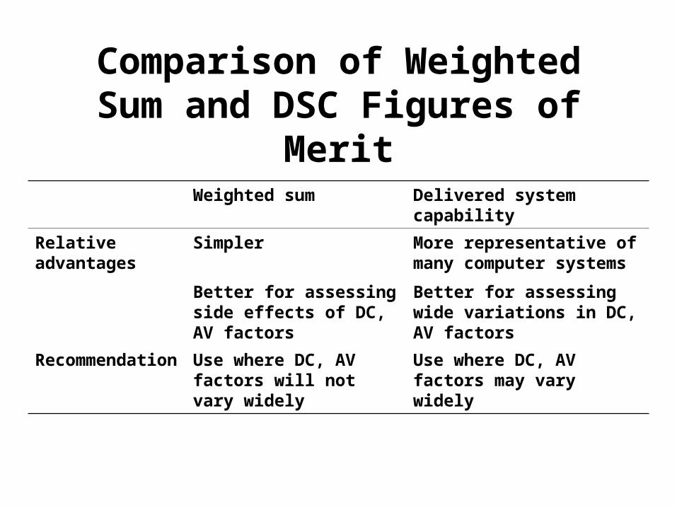
Comparison of Weighted Sum and DSC Figures of Merit

Weighted sum Delivered system capability

Relative advantages

Simpler More representative of many computer systems

Better for assessing side effects of DC, AV factors

Better for assessing wide variations in DC, AV factors

Recommendation Use where DC, AV factors will not vary widely

Use where DC, AV factors may vary widely