Chapter15 Approximations for Probability Distributions and ...€¦ · Chapter15 Approximations for...

Chapter 15Approximations for Probability Distributionsand Stochastic Optimization Problems

Georg Ch. Pflug and Alois Pichler

Abstract In this chapter, an overview of the scenario generation problem is given.After an introduction, the basic problem of measuring the distance between twosingle-period probability models is described in Section 15.2. Section 15.3 dealswith finding good single-period scenarios based on the results of the first section.The distance concepts are extended to the multi-period situation in Section 15.4.Finally, Section 15.5 deals with the construction and reduction of scenario trees.

Keywords Scenario generation · Probability distances · Optimal discretizations ·Scenario trees · Nested distributions

15.1 Introduction

Decision making under uncertainty is based upon

(i) a probability model for the uncertain values,(ii) a cost or profit function depending on the decision variables and the uncertain-

ties, and(iii) a probability functional, like expectation, median, etc., to summarize the ran-

dom costs or profits in a real-valued objective.

We describe the decision model under uncertainty by

(Opt) max{F(x) = AP [H(x, ξ)] : x ∈ X}, (15.1)

where H(·, ·) denotes the profit function, with x the decision and ξ the randomvariable or random vector modeling uncertainty. Both – the uncertain data ξ andthe decision x – may be stochastic processes adapted to some filtration FF . A isthe probability functional and X is the set of constraints. P denotes the underlyingprobability measure.

G. Ch. Pflug (B)Department of Statistics and Operations Research, University of Vienna A-1010,Wien – Vienna, Austriae-mail: [email protected]

M. Bertocchi et al. (eds.), Stochastic Optimization Methods in Finance and Energy,International Series in Operations Research & Management Science 163,DOI 10.1007/978-1-4419-9586-5_15, C© Springer Science+Business Media, LLC 2011

343

344 G. Ch. Pflug and A. Pichler

The most difficult part in establishing a formalized decision model of type (15.1)for a real decision situation is to find the probability model P . Typically, there isa sample of past data available, but not more. It needs two steps to come from thesample of observations to the scenario model:

(1) In the first step a probability model is identified, i.e., the description of theuncertainties as random variables or random processes by identifying the prob-ability distribution. This step is based on statistical methods of model selectionand parameter estimation. If several probability measures represent the dataequally well, one speaks of ambiguity. In the non-ambiguous situation, one andonly one probability model is selected and this model is the basis for the nextstep.

(2) In the following scenario generation step, a scenario model is found, whichis an approximation of (15.1) by a finite model of lower complexity than theprobability model.

The scenario model differs from the original model (15.1) insofar as P is replacedby P , but – especially in multi-period problems – also the feasible set X is replacedby a smaller, feasible set X:

(Opt) max{F(x) = AP [H(x, ξ)] : x ∈ X}. (15.2)

It is essential that the scenario model is finite (i.e., only finitely many valuesof the uncertainties are possible), but a good approximation to the original modelas well. The finiteness is essential to keep the computational complexity low, andthe approximative character is needed to allow the results to be carried over to theoriginal model. In some cases, which do not need to be treated further here, finitelymany scenarios are given right from the beginning (e.g., Switzerland will join theEU in 2015 – yes or no, or UK will adopt the EURO in 2020 and so on). The sameis true, if the scenarios are just taken as the historic data without further transforma-tion or information reduction. However, the justification of using just the empiricalsample as the scenario model lies in the fact that these samples converge to thetrue underlying distribution if the sample size increases. For a quantification of thisstatement see Section 15.3.3 on Monte Carlo approximation below.

When stressing the approximative character of a scenario model we have to thinkabout the consequences of this approximation and to estimate the error committedby replacing the probability model by the scenario model. Consider the diagrambelow: It is typically impossible to solve problem (15.1) directly due to its complex-ity. Therefore, one has to go around this problem and solve the simplified problem(15.2). Especially for multi-period problems, the solution of the approximate prob-lem is not directly applicable to the original problem, but an extension function isneeded, which extends the solution of the approximate problem to a solution of

15 Approximations for Probability Distributions and Stochastic Optimization . . . 345

the original problem. Of course, the extended solution of the approximate problemis typically suboptimal for the original problem. The respective gap is called theapproximation error. It is the important goal of scenario generation to make this gapacceptably small.

The quality of a scenario approximation depends on the distance between the orig-inal probability P and the scenario probability P . Well-known quantitative stabil-ity theorems (see, e.g., Dupacova (1990), Heitsch et al. (2006), and Rachev andRoemisch (2002)) establish the relation between distances of probability models onone side and distances between optimal values or solutions on the other side (see,e.g., cite stability). For this reason, distance concepts for probability distributionson R

M are crucial.

15.2 Distances Between Probability Distributions

Let P be a set of probability measures on RM .

Definition 1.1 A semi-distance on P is a function d(·, ·) on P × P , which satisfies(i) and (ii) as follows:

(i) Nonnegativity: For all P1, P2 ∈ P

d(P1, P2) ≥ 0.

(ii) Triangle inequality: For all P1, P2, P3 ∈ P

d(P1, P2) ≤ d(P1, P3)+ d(P3, P2).

If a semi-distance satisfies the strictness property

(iii) Strictness: If d(P1, P2) = 0, then P1 = P2,it is called a distance.


A general principle for defining semi-distances and distances consists in choos-ing a family of integrable functions H (i.e., a family of functions such that theintegral

∫h(w) d P(w) exists for all P ∈ P) and defining

dH(P1, P2) = sup

{|∫

h(w) dP1(w)−∫

h(w) dP2(w)| : h ∈ H}.

We call dH the (semi-)distance generated by H.In general, dH is only a semi-distance. If H is separating, i.e., if for every pair

P1, P2 ∈ P there is a function h ∈ H such that∫

h dP1 �=∫

h dP2, then dH is adistance.

15.2.1 The Moment-Matching Semi-Distance

Let Pq be the set of all probability measures on R1 which possess the qth moment,

i.e., for which∫

max(1, |w|q) d P(w) < ∞. The moment-matching semi-distanceon Pq is

dMq (P1, P2) = sup

{|∫ws dP1(w)−

∫ws dP2(w)| : s ∈ {1, 2, . . . , q}

}.

(15.3)The moment-matching semi-distance is not a distance, even if q is chosen to be largeor even infinity. In fact, there are examples of two different probability measures onR

1, which have the same moments of all orders. For instance, there are probabilitymeasures, which have all moments equal to those of the lognormal distribution, butare not lognormal (see, e.g., Heyde (1963)).

A widespread method is to match the first four moments (Hoyland and Wallace2001), i.e., to work with dM4 . The following example shows that two densities coin-ciding in their first four moments may exhibit very different properties.

Example Let P1 and P2 be the two probability measures with densities g1 and g2where

g1(x) = 0.39876 [ exp(−|x + 0.2297|3)1l{x≤−1.2297}+ exp(−|x + 0.2297|)1l{−1.2297<x≤−0.2297}+ exp(−0.4024 · (x + 0.2297))1l{−0.2297<x≤2.2552}+ 1.09848 · (0.4024x + 0.29245)−61l{2.2552<x}],

g2(x) = 0.5962 1l{|x |≤0.81628} + 0.005948 1l{0.81628<|x |≤3.05876}.

Both densities are unimodal and coincide in the first four moments, which arem1 = 0, m2 = 0.3275, m3 = 0, m4 = 0.72299 (mq(P) =

∫wq d P(w)). The

fifth moments, however, could not differ more: While P1 has infinite fifth moment,the fifth moment of P2 is zero. Density g1 is asymmetric, has a sharp cusp at the


point −0.2297 and unbounded support. In contrast, g2 is symmetric around 0, hasa flat density there, has finite support, and possesses all moments. The distributionfunctions and quantiles differ drastically: We have that G P1(0.81) = 0.6257 andG P1(−0.81) = 0.1098, while G P2(0.81) = 0.9807 and G P2(−0.81) = 0.0133.Thus the probability of the interval [−0.81, 0.81] is only 51% under P1, while it is96% under P2.

−4 −3 −2 −1 0 1 2 3 40

0.1

0.2

0.3

0.4

0.5

0.6

0.7

Two densities g1 and g2 with identical first four moments.

−5 0 50

0.1

0.2

0.3

0.4

0.5

0.6

0.7

0.8

0.9

1

The two pertaining distribution functions G1 and G2.

Summarizing, the moment matching semi-distance is not well suited for scenarioapproximation, since it is not fine enough to capture the relevant quality of approx-imation.


The other extreme would be to choose as the generating class H all measurablefunctions h such that |h| ≤ 1. This class generates a distance, which is called thevariational distance (more precisely twice the variational distance). It is easy to seethat if P1 resp. P2 have densities g1 resp. g2 w.r.t. λ, then

sup

{∫h dP1 −

∫h dP2 : |h| ≤ 1, h measurable

}

=∫|g1(x)− g2(x)| dλ(x)

= 2 sup{|P1(A)− P2(A) : A measurable set}.

We call

dV (P1, P2) = sup{|P1(A)− P2(A)| : A measurable set} (15.4)

the variational distance between P1 and P2.The variational distance is a very fine distance, too fine for our applications: If P1

has a density and P2 sits on at most countably many points, then dV (P1, P2) = 1,independently on the number of mass points of P2. Thus there is no hope to approx-imate any continuous distribution by a discrete one w.r.t. the variational distance.

One may, however, restrict the class of sets in (15.4) to a certain subclass. Ifone takes the class of half-unbounded rectangles in R

M of the form (−∞, t1] ×(−∞, t2] × · · · × (−∞, tM ] one gets the uniform distance, also called Kolmogorovdistance

dU (P1, P2) = sup{|G P1(x)− G P2(x)| : x ∈ RM }, (15.5)

where G P (t) is the distribution function of P ,

G P (t) = P{(−∞, t1] × · · · × (−∞, tM ]}.

The uniform distance appears in the Hlawka–Koksma inequality:

∫h(u) dP1(u)−

∫h(u) dP2(u) ≤ dU (P1, P2) · V (h), (15.6)

where V (h) is the Hardy–Krause variation of h. In dimension M = 1, V is the usualtotal variation

V (h) = sup

{∑i

|h(zi )− h(zi−1)| : z1 < z2 < · · · < zn, n arbitrary

}.

In higher dimensions, let V (M)(h) = sup∑

J1,...,Jn is a partition by rectangles Ji|�Ji (h)|, where

�J (h) is the sum of values of h at the vertices of J , where adjacent vertices get


opposing signs. The Hardy–Krause variation of h is defined as∑M

m=1 V (m)(h). dU

is invariant w.r.t. monotone transformations, i.e., if T is a monotone transformation,then the image measures PT

i = Pi ◦ T−1 satisfy

dU (PT1 , PT

2 ) = dU (P1, P2).

Notice that a unit mass at point 0 and at point 1/n are at a distance 1 both in thedU distance, for any even large n. Thus it may be felt that also this distance is toofine for good approximation results. A minimal requirement of closedness is thatintegrals of bounded, continuous functions are close and this leads to the notion ofweak convergence.

Definition 1.2 (Weak convergence) A sequence of probability measures Pn on RM

converges weakly to P (in symbol Pn ⇒ P), if

∫h dPn →

∫h dP

as n → ∞, for all bounded, continuous functions h. Weak convergence is themost important notion for scenario approximation: We typically aim at constructingscenario models which, for increasing complexity, finally converge weakly to theunderlying continuous model.

If a distance d has the property that

d(Pn, P)→ 0 if and only if Pn ⇒ P

we say that d metricizes weak convergence.The following three distances metricize the weak convergence on some subsets

of all probability measures on RM :

(i) The bounded Lipschitz metric: If H is the class of bounded functions withLipschitz constant 1, the following distance is obtained:

dBL(P1, P2) = sup

{∫h dP1 −

∫hdP2 : |h(u)| ≤ 1, L1(h) ≤ 1

}, (15.7)

where

L1(h) = inf{L : |h(u)− h(v)| ≤ L‖u − v‖}.

This distance metricizes weak convergence for all probability measures on RM .

(ii) The Kantorovich distance: If one drops the requirement of boundedness of h,one gets the Kantorovich distance


dKA(P1, P2) = sup

{∫h dP1 −

∫h dP2 : L1(h) ≤ 1

}. (15.8)

This distance metricizes weak convergence on sets of probability measureswhich possess uniformly a first moment. (A set P of probability measureshas uniformly a first moment, if for every ε there is a constant Cε such that∫‖x‖>Cε

‖x‖ dP(x) < ε for all P ∈ P .) See the review of Gibbs and Su (2002).On the real line, the Kantorovich metric may also be written as

dKA(P, P) =∫|G P (u)− G P (u)| du =

∫|G−1

P (u)− G−1P(u)| du,

where G−1P (u) = sup{v : G P (v) ≤ u} (see Vallander (1973)).

(iii) The Fortet–Mourier metric: If H is the class of Lipschitz functions of order q,the Fortet–Mourier distance is obtained:

dFMq (P1, P2) = sup

{∫h dP1 −

∫hdP2 : Lq(h) ≤ 1

}, (15.9)

where the Lipschitz constant of order q is defined as

Lq(h) = inf{L : |h(u)− h(v)| ≤ L||u − v||max(1, ||u||q−1, ||v||q−1)}.(15.10)

Notice that Lq(h) ≤ Lq ′(h) for q ′ ≤ q. In particular, Lq(h) ≤ L1(h) for all q ≥ 1and therefore

dFMq (P1, P2) ≥ dFMq′ (P1, P2) ≥ dKA(P1, P2).

The Fortet–Mourier distance metricizes weak convergence on sets of probabilitymeasures possessing uniformly a qth moment. Notice that the function u �→ ‖u‖qis q-Lipschitz with Lipschitz constant Lq = q. On R

1, the Fortet–Mourier distancemay be equivalently written as

dFMq (P1, P2) =∫

max(1, |u|q−1)|G P1(u)− G P2(u)| du

(see Rachev (1991), p. 93). If q = 1, the Fortet–Mourier distance coincides with theKantorovich distance.

The Kantorovich distance is related to the mass transportation problem (Monge’sproblem – Monge (1781), see also Rachev (1991), p. 89) through the followingtheorem.


Theorem 1.3 (Kantorovich–Rubinstein)

dKA(P1, P2) = inf{E(|X1 − X2|) : s.t. the joint distribution (X1, X2)

is arbitrary, but the marginal distributions are fixed

such thatX1 ∼ P1, X2 ∼ P2} (15.11)

(see Rachev (1991), theorems 5.3.2 and 6.1.1).

The infimum in (15.11) is attained. The optimal joint distribution (X1, X2) describeshow masses with distribution P should be transported with minimal effort to yieldthe new mass distribution P . The analogue of the Hlawka–Koksma inequality ishere

∫|h(u) dP1(u)−

∫h(u) dP2(u)| ≤ dKA(P1, P2) · L1(h). (15.12)

The Kantorovich metric can be defined on arbitrary metric spaces R with metric d:If P1 and P2 are probabilities on this space, then dKA(P1, P2; d) is defined by

dKA(P1, P2; d) = sup

{∫h dP1 −

∫h dP2 : |h(u)− h(v)| ≤ d(u, v)

}.

(15.13)Notice that the metric d(·, ·; d) is compatible with the metric d in the followingsense: If δu resp. δv are unit point masses at u resp. v, then

dKA(δu, δv; d) = d(u, v).

The theorem of Kantorovich–Rubinstein extends to the general case:

dKA(P1, P2; d) = inf{E[d(X1, X2)] : where the joint distribution (X1, X2)

is arbitrary, but the marginal distributions are fixed

such that X1 ∼ P1, X2 ∼ P2}. (15.14)

A variety of Kantorovich metrics may be defined, if RM is endowed with differ-

ent metrics than the Euclidean one.

15.2.2 Alternative Metrics on RM

By (15.13), to every metric d on RM , there corresponds a distance of the Kan-

torovich type. For instance, let d0 be the discrete metric

d0(u, v) ={

1 if u �= v,0 if u = v.


The set of all Lipschitz functions w.r.t. the discrete metric coincides with the setof all measurable functions h such that 0 ≤ h ≤ 1 or its translates. Consequentlythe pertaining Kantorovich distance coincides with the variational distance

dKA(P1, P2; d0) = dV (P1, P2).

Alternative metrics on R1 can, for instance, be generated by nonlinear transform

of the axis. Let χ be any bijective monotone transformation, which maps R1 into

R1. Then d(u, v) := |χ(u) − χ(v)| defines a new metric on R

1. Notice that thefamily functions which are Lipschitz w.r.t the distance d and the Euclidean distance|u − v| may be quite different.

In particular, let us look at the bijective transformations (for q > 0)

χq(u) ={

u |u| ≤ 1

|u|q sgn(u) |u| ≥ 1.

Notice that χ−1q (u) = χ1/q(u). Introduce the metric dχq (u, v) = |χq(u)−χq(v)|.

We remark that dχ1(u, v) = |u − v|. Denote by dKA(·, ·; dχq ) the Kantorovich dis-tance which is based on the distance dχq ,

dKA(P1, P2; dχq ) = sup

{∫h dP1 −

∫h dP2 : ‖h(u)− h(v)‖ ≤ dχq (u, v)

}.

Let Pχq be the image measure of P under χq , that is Pχq assigns to a set A thevalue P{χ1/q(A)}. Notice that Pχq has distribution function

G Pχq (x) = G P (χ1/q(x)).

This leads to the following identity:

dKA(P1, P2; dχq ) = dKA(Pχq1 , P

χq2 ; | · |).

It is possible to relate the Fortet–Mourier distance dMq to the distance dKA(·, ·; dχq ).To this end, we show first that

Lq(h ◦ χq) ≤ q · L1(h) (15.15)

and

L1(h ◦ χ1/q) ≤ Lq(h). (15.16)

If L1(h) <∞, then

|h(χq(u))− h(χq(v))| ≤ L1(h)|χq(u)− χq(v)|≤ L1(h) · q ·max(1, |u|q−1, |v|q−1)|u − v|


which implies (15.15). On the other hand, if Lq(h) <∞, then

|h(χ1/q(u))− h(χ1/q(v))|≤ Lq(h)max(1, |χ1/q(u)|q−1, |χ1/q(v)|q−1)|χ1/q(u)− χ1/q(v)|≤ Lq(h)max(1,max(|u|, |v|)q−1)max(1,max(|u|, |v|)(1−q)/q |u − v|≤ Lq(h)|u − v|

and therefore (15.16) holds. As a consequence, we get the following relations:

1

qdKA(P1, P2; dχq ) =

1

qdKA(G P1 ◦ χ1/q ,G P2 ◦ χ1/q)

≤ dFMq (P1, P2)

≤ dKA(G P1 ◦ χ1/q ,G P2 ◦ χ1/q) = dKA(P1, P2; dχq ). (15.17)

Thus one sees that it is practically equivalent to measure the distance by the Fortet–Mourier distance of order q or by the Kantorovich distance (i.e., the Fortet–Mourierdistance of order 1) but with the real line endowed with the metric dχq .

15.2.3 Extending the Kantorovich Distance to the WassersteinDistance

By the Kantorovich–Rubinstein Theorem, the Kantorovich metric is the optimalcost of a transportation problem. If the cost function is not the distance d itself, buta power dr of it, we are led to the Wasserstein metric dW,r .

dW,r (P1, P2; d)r = inf

{∫d(x1, x2)

rπ(dx1, dx2); s.t. the joint probability

measure π has marginals such that

π(A × RM ) = P1(A) and π(RM × B) = P2(B)

}. (15.18)

This is a metric for r ≥ 1. For r < 1, the Wasserstein distance is defined as

dW,r (P1, P2; d) = inf

{∫d(x1, x2)

rπ(dx1, dx2); where the joint probability



}(15.19)

(see Villani (2008)).


15.2.4 Notational Convention

When there is no doubt about the underlying distance d, we simply write

dr (P1, P2) instead of dW,r (P1, P2; d).

Recall that in this notation, the Kantorovich distance is dKA(P1, P2) = d1(P1, P2).

15.2.5 Wasserstein Distance and Kantorovich Distanceas Linear Program

To compute the Wasserstein distance for discrete probability distributions amountsto solving a linear program, as we shall outline here:

Consider the discrete measures P :=∑s psδzs and Q :=∑

t qtδz′t and – withinthis setting – the problem

Minimize(in π)

∑s,tπs,t cs,t

subject to∑

tπs,t = ps,

∑sπs,t = qt and

πs,t ≥ 0,

(15.20)

where cs,t := d(zs, z′t

)r is a matrix derived from the general distance function d.This matrix c represents the weighted costs related to the transportation of massesfrom zs to z′t .

Notice that (15.20) is a general linear program, which is already well defined byspecifying the cost matrix cs,t and the probability masses ps and qt . So in particularthe mass points zs are not essential to formulate the problem; they may representabstract objects.

Observe further that

∑s,t

πs,t =∑

s

ps =∑

t

qt = 1,

thus π is a probability measure, representing – due to the constraints – a transportplan from P to Q. The linear program (15.20) thus returns the minimal distancebetween those measures, and as a minimizing argument the optimal transport planin particular for transporting masses from object zs to z′t .

The linear program (15.20) has a dual with vanishing duality gap. The theoremof Kantorovich–Rubinstein allows to further characterize (in the situation r = 1) thedual program; it amounts to just finding a Lipschitz-1 function h which maximizesthe respective expectation:


Maximize(in h)

∑s pshs −∑

t qt ht ,

subject to hs − ht ≤ d (zs, zt ) .

Due to the vanishing duality gap the relation

∑s

psh∗s −∑

t

qt h∗t =

∑s,t

π∗s,t cs,t

holds true, where h∗ is the optimal Lipschitz-1 function and π∗ the optimal jointmeasure.

15.2.6 Bibliographical Remarks

The distance dKA was introduced by Kantorovich in 1942 as a distance in gen-eral spaces. In 1948, he established the relation of this distance (in R

n) to themass transportation problem formulated by Gaspard Monge in 1781. In 1969,L. N. Wasserstein – unaware of the work of Kantorovich – reinvented this dis-tance for using it for convergence results of Markov processes and 1 year laterR. L. Dobrushin used and generalized this distance and initiated the name Wasser-stein distance. S. S. Vallander studied the special case of measures in R

1 in 1974and this paper made the name Wasserstein metric popular. The distance dU wasintroduced by Kolmogorov in 1933. It is often called Kolmogorov distance.

15.3 Single-Period Discretizations

In this section, we study the discrete approximation problem:Let a probability measure P on R

M be given. We want to find a probabilitymeasure sitting on at most S points, such that some distance d(P, P) is small.

We say “small” and not “minimal”, since it may be computationally intractableto really find the minimum. Formally, define PS as the family of all probabilitymeasures

P =S∑

s=1

psδzs

on RM sitting on at most S points. Here δz denotes the point mass at point z. We try

to find a P ∈ PS such that

d(P, P) is close to min{d(P, Q) : Q ∈ PS}.

There are several methods to attack the problem, which we order in decreasing orderof computational effort and as well in decreasing order of approximation quality (seeFig. 15.1):


Fig. 15.1 Methods of scenario generation

While the probability measure P may have a density or may be discrete, the mea-sure P is always characterized by the list of probability masses ps, s = 1, . . . , S andthe list of mass points zs, s = 1, . . . , S. The discrete measure P is represented by

P =[

p1 p2 · · · pS

z1 z2 · · · zS .

].

The approximation problem depends heavily on the chosen distance d, as will beseen. We treat the optimal quantization problem in Section 15.3.1, the quasi-MonteCarlo technique in Section 15.3.2 and the Monte Carlo technique in Section 15.3.3.Some quantization heuristics are contained in Chapter 3.

15.3.1 Optimal and Asymptotically Optimal Quantizers

The basic approximation problem, i.e., to approximate a distribution on RM by a

distribution sitting on at most S points leads to a non-convex optimization prob-lem. To find its global solution is computationally hard. Moreover, no closed-formsolution is known, even for the simplest distributions.

Recall the basic problem: Let d be some distance for probability measures andlet PS be the family of probability distributions sitting on at most S points. For agiven probability P ∈ PS , the main question is to find the quantization error

qS,d(P) = inf{d(P, Q) : Q ∈ PS} (15.21)

and the optimal quantization set

QS,d(P) = argmin {d(P, Q) : Q ∈ PS} (15.22)

(if it exists).


15.3.1.1 Optimal Quantizers for Wasserstein Distances dr

Since all elements P of PS are of the form P = ∑Ss=1 psδzs , the quantization

problem consists essentially of two steps:

(1) Find the optimal supporting points zs .(2) Given the supporting points zs , find the probabilities ps , which minimize

dr

(P,

S∑s=1

psδzs

)(15.23)

for the Wasserstein distance.

Recall the Wasserstein dr distances contain the Kantorovich distance as the specialcase for r = 1.

We show that the second problem has an easy solution for the chosen distance:Let z = (z1, . . . , zS) be the vector of supporting points and suppose that they are alldistinct. Introduce the family of Voronoi diagrams V(z) as the family of all partitions(A1, . . . , AS), where As are pairwise disjoint and R

M =⋃Ss=1 As , such that

As ⊆ {y : d(y, zs) = mink

d(y, zk)}.

Then the possible optimal probability weights ps for minimizing

dr

(P,

∑Ss=1 psδzs

)can be found by

p = (p1, . . . , pS), where ps = P(As); (A1, . . . , AS) ∈ V(z).

The optimal probability weights are unique, iff

P{y : d(y, zs) = d(y, zk), for some s �= k} = 0.

One may also reformulate (15.23) in terms of random variables: Let X ∼ P andlet X be a random variable which takes only finitely many values X ∈ {z1, . . . , zS},then

Ddr (z) := inf{E[d(X, X)r ] : X ∼ P, X ∈ {z1, . . . , zS}}= inf{dr (P, P)r : supp(P) ⊆ {z1, . . . , zS}}=

∫min

sd(x, zs)

r dP(x).

Unfortunately, the function z �→ Ddr (z) is non-convex and typically has multiplelocal minima. Notice that the quantization error defined in (15.21) satisfies

qS,dr (P) = min{[Ddr (z)]1/r : z = (z1, . . . , zS)}.


Lemma 2.1 The mapping P �→ qS,dr (P) is concave.

Proof Let P =∑Ii=1wi Pi for some positive weights with

∑Ii=1wi = 1. Then

qS,dr (P) =I∑

i=1

wi

∫min

s[d(x, zs)]r dPi (x) ≥

I∑i=1

wi qS,dr (Pi ).

!"Lemma 2.2 Let

∑Ii=1 Si ≤ S and the weights wi as above. Then

qS,dr

(I∑

i=1

wi Pi

)≤

I∑i=1

wi qSi ,dr (Pi ).

Proof Let Pi such that dr (Pi , Pi ) = qSi ,dr (P). Then

qS,dr

(I∑

i=1

wi Pi

)≤ dr

(I∑

i=1

wi Pi ,

I∑i=1

wi Pi

)≤

I∑i=1

wi qSi ,dr (Pi ).

!"For the next lemma, it is necessary to specify the distance d to

dr (x, y) =[

M∑m=1

|xrm − yr

m |]1/r

.

Lemma (Product quantizers) Let∏I

i=1 Si ≤ S. Then

qS,dr (⊗Ii=1 Pi ) ≤

I∑i=1

qS,dr (Pi ).

Proof Let Pi ∈ PS such that dr (Pi , Pi ) = qSi ,dr (P). Then

qS,dr (⊗Ii=1 Pi ) ≤ dr (⊗I

i=1 Pi ,⊗Ii=1 Pi ) =

I∑i=1

qSi ,dr (Pi ).

!"

15.3.1.2 Interpretation as Facility Location Problems on R

On R1 one may w.l.o.g. assume that the points zs are in ascending order

z1 ≤ z2 ≤ · · · ≤ zS . The pertaining Voronoi tessellation then is

Vs = (bs−1, bs], s = 1, . . . S,


with b0 = −∞, bS = +∞ and for 1 ≤ s ≤ S; the points bs are chosen such thatd(bs, zs) = d(bs, zs+1), and the optimal masses are then ps = G(bs) − G(bs−1).For the Euclidean distance on R, the bs’s are just the midpoints

zs = 1

2(bs−1 + bs), s = 1, . . . , S.

In this case, the Wasserstein distance is

dr (P, P)r =S∑

s=1

∫ zs+zs+12

zs−1+zs2

|u − zs |r dG(u), (15.24)

with z0 = −∞ and zS+1 = +∞.While step (2) of (15.23) is easy, step (1) is more involved: Let, for z1 ≤ z2

≤ · · · ≤ zS ,

D(z1, . . . , zS) =∫

mins

d(x, zs)r dG(x) (15.25)

The global minimum of this function is sought for. Notice that D is non-convex,i.e., the global minimization of D is a hard problem. The function D can be viewedas the travel mean costs of customers distributed along the real line with d.f. G totravel to the nearest location of one of the facilities, placed at z1, . . . , zS , if the travelcosts from u to v are d(u, v)r .

Facility Location The problem of minimizing the function D in (15.25) is aninstance of the classical Weber location problem, which was introduced by A. Weberin 1909 (English translation published 1929 (Weber 1929)). A recent state-of-the-artoverview of the theory and applications was published by Drezner and Hamacher(2002).

Explicit Optimal Solutions Only in exceptional cases explicit solutions of theoptimal quantization problems (15.21) resp. (15.22) are known. Here are someexamples; for more details, see Graf and Luschgy (2000).

Example (The Laplace distribution in R1) For the Euclidean distance on R and

the Laplace distribution with density f (x) = 12 exp(−|x |), the optimal supporting

points for even S = 2k are

zs =

⎧⎪⎪⎪⎪⎨⎪⎪⎪⎪⎩

2 log

(s√

k2+k

), 1 ≤ s ≤ k,

2 log

(√k2+k

S+1−s

), k + 1 ≤ s ≤ S.

The quantization error is


qS,d1(P) ={

log(

1+ 2S

), S even ,

2S+1 , S odd.

Example (The Exponential distribution in R1) For the Euclidean distance on R

and the Exponential distribution with density f (x) = exp(−x)1lx≥0, the optimalsupporting points are

zs = 2 log

( √S2 + S

S + 1− s

); s = 1, . . . , S.

The quantization error is

qS,d1(P) = log

(1+ 1

S

).

Example (The uniform distribution in RM ) To discuss the uniform distribution in

higher dimension, it is necessary to further specify the distance on the sample space:

As distances on RM we consider the p-norms dp(u, v) =

[∑Mm=1 |um − vm |p

]1/p

for 1 ≤ p <∞ resp. d∞(u, v) = max1≤m≤M |um − vm |.Based on dp, we consider the Wasserstein distances dp,r

dp,r (P1, P2)r = inf

{∫dp(x1, x2)

rπ(dx1, dx2); where the joint probability



}. (15.26)

Let q(M)S,dp,r:= qS,dp,r (U[0, 1]M ) be the minimal error of approximation to the

uniform distribution on the M-dimensional unit cube [0, 1]M . The exact values areonly known for

q(M)1,dp,r=

⎧⎪⎨⎪⎩

M(1+r)2r , 1 ≤ p <∞,

M(M+r)2r , p = ∞

and

q(M)1,d∞,r =M

(M + r)2r.

15.3.1.3 Asymptotically Optimal Quantizers

In most cases, the solutions of (15.21) and (15.22) are unknown and cannot beexpressed in an analytic way. Therefore one may ask the simpler “asymptotic”questions:


• What is the rate in which qS,dr (P) converges to zero as S tends to infinity?• Is there a constructive way to find a sequence being asymptotically optimal, i.e.,

a sequence (P+S ) such that

d(P, P+S )qS,dr (P)

→ 1

as S→∞?

To investigate these questions introduce the quantities

q(M)dp,r:= inf

SSr/M qS,dp,r (U[0, 1]M ), (15.27)

qdp,r (P) := infS

Sr/M qS,dp,r (P),

where U[0, 1]M is the uniform distribution on the M-dimensional unit cube [0, 1]M .It deduces from the concavity of P �→ qS,dr,p (P) that the mappings P �→

qdp,r (P) are concave as well.

The quantities q(M)dp,rare found to be universal constants; however, they are known

in special cases only:

• q(1)dp,r= 1(1+r)2r ,

• q(M)d∞,r = M(M+r)2r .

The next theorem links a general distribution P with the uniform distribution, pro-viding a relation between qdp,r (P) and q(M)dp,r

. As for a proof we refer the reader toGraf and Luschgy (2000), theorem 6.2. or Na and Neuhoff (1995).

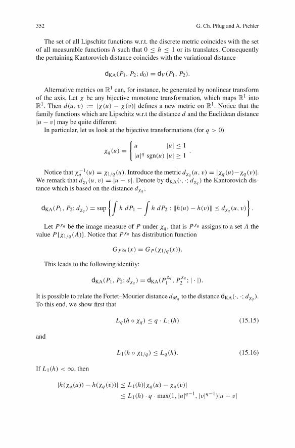
Theorem (Zador–Gersho formula) Suppose that P has a density g with∫ |u|r+δg(u) du <∞ for some δ > 0. Then

qdp,r (P) = infS

Sr/M qS,dp,r (P) = q(M)dp,r·[∫

RMg(x)

MM+r dx

] M+rM

, (15.28)

where q(M)dp,ris given by (15.27).

For the real line, this specializes to

qdp,r (P) =1

(1+ r)2r

(∫R

g(u)1

1+r du

)1+r

for all p, since all distances dp are equal for M = 1. Specializing further to r = 1,one gets


qdp,1(P) =1

4

(∫R

√g(u) du

)2

.

Heuristics The Zador–Gersho formula (15.28), together with identity (15.24) give

rise that the optimal, asymptotic point density for zs is proportional to gM

M+r . In R1

again this translates to solving the quantile equations

∫ zs

−∞g

11+r (x) dx = 2s − 1

2S·∫ ∞−∞

g1

1+r (x) dx

for s = 1, 2, . . . S and then to put

ps :=∫ zs+zs+1

2

zs−1+zs2

g(x) dx

as above. It can be proved that the points zs specified accordingly are indeed asymp-totically optimal and in practice this has proven to be a very powerful setting.

Example If P is the univariate normal distribution N (μ, σ 2), then qdp,1(N (μ, σ ) =σ√π2 . For the M-dimensional multivariate normal distribution N (μ,�) one finds

that

qdp,r (N (μ,�) = q(M)dp,r(2π)r/2

(M + r

M

)(M+r)/2

(det�)r/(2M).

15.3.1.4 Optimal Quantizers for the Uniform (Kolmogorov) Distance

In dimension M = 1, the solution of the uniform discrete approximation problem iseasy: Notice that the uniform distance is invariant w.r.t. monotone transformations,which means that the problem can be mapped to the uniform distribution via thequantile transform and then mapped back.

The uniform distribution U[0, 1] is optimally approximated by

P =[

1/S 1/S 1/S · · · 1/S1

2S3

2S5

2S · · · 2S−12S

]

and the distance is

dU (U[0, 1], P) = 1/S.

For an arbitrary P with distribution function G, the optimal approximation is given(by virtue of the quantile transform) by


zs = G−1(

2s − 1

2S

), s = 1, . . . , S,

ps = 1/S, s = 1, . . . , S.

The distance is bounded by 1/S. If G is continuous, then the distance is exactlyequal to 1/S. In this case, the uniform distance approximation problem leads alwaysto approximating distributions, which put the same mass 1/S at all mass points.This implies that the tails of P are not well represented by P . This drawback is notpresent when minimizing the Kantorovich distance.

15.3.1.5 Heavy Tail Control

Minimizing the Kantorovich distance minimizes the difference in expectation for allLipschitz functions. However, it may not lead to a good approximation for highermoments or even the variance. If a good approximation of higher moments is alsorequired, the Fortet–Mourier distance may be used.

Another possibility, which seems to be even more adapted to control tails, isto choose the Wasserstein r -distance instead of the Kantorovich distance for someappropriately chosen r > 1.

To approximate tails and higher moments are necessary for many real-worldapplications especially in the area of financial management.

Example Suppose we want to approximate the t-Student distribution P with 2degrees of freedom, i.e., density (2+ x2)−3/2 by a discrete distribution sitting on 5points. The optimal approximation with the uniform distance is

P1 =[

0.2 0.2 0.2 0.2 0.2−1.8856 −0.6172 0 0.6172 1.8856

],

while minimizing the Kantorovich distance, the approximated distribution is

P2 =[

0.0446 0.2601 0.3906 0.2601 0.0446−4.58 −1.56 0 1.56 4.58

].

These results can be compared visually in Fig. 15.2 where one can see clearly thatthe minimization of the Kantorovich distance leads to a much better approximationof the tails.

But even this approximation can be improved by heavy tail control: Applyingthe stretching function χ2 to the t-distribution, one gets the distribution with density(Fig. 15.3)

{(2+ x2)−3/2 if |x | ≤ 1,

12√

x(2+ |x |)−3/2 if |x | > 1.


−6 −4 −2 0 2 4 60

0.05

0.1

0.15

0.2

0.25

0.3

0.35

0.4

−6 −4 −2 0 2 4 60

0.05

0.1

0.15

0.2

0.25

0.3

0.35

0.4

Fig. 15.2 Approximation of the t (2)-distribution: uniform (left) and Kantorovich (right)

−6 −4 −2 0 2 4 60

0.05

0.1

0.15

0.2

0.25

0.3

0.35

0.4

−6 −4 −2 0 2 4 60

0.05

0.1

0.15

0.2

0.25

0.3

0.35

0.4

Fig. 15.3 Approximation of the t (2)-distribution: Kantorovich with Euclidean distance (left) andKantorovich with distorted distance dχ2 (right)

This distribution has heavier tails than the original t-distribution. Weapproximate this distribution w.r.t the Kantorovich distance by a 5-point distributionand transform back the obtained mass points using the transformation χ1/2 to get

P =[

0.05 0.2 0.5 0.2 0.05−4.8216 −1.6416 0 1.6416 4.8216

].

Compared to the previous ones, this approximation has a better coverage of thetails. The second moment is better approximated as well.

15.3.2 Quasi-Monte Carlo

As above, let U[0, 1]M be the uniform distribution on [0, 1]M and let PS =1S

∑Ss=1 δzs . Then the uniform distance dU (U[0, 1]M , PS) is called the star discrep-

ancy D∗S(z1, . . . , zS) of (z1, . . . , zS)


D∗S(z1, . . . , zS) = sup

{1

S

S∑s=1

1l{[0,a1]×···×[0,aM ]}(zs)−M∏

m=1

am : 0 < am ≤ 1

}.

(15.29)

A sequence z = (z1, z2, . . . ) in [0, 1]M is called a low-discrepancy sequence, if

lim supS→∞

S

log(S)MD∗S(z1, . . . , zS) <∞,

i.e., if there is a constant C such that for all S,

D∗S(z) = D∗S(z1, . . . , zS) ≤ Clog(S)M

S.

A low-discrepancy sequence allows the approximation of the uniform distribu-tion in such a way that

dU (U[0, 1]M , PS) ≤ Clog(S)M

S.

Low-discrepancy sequences exist. The most prominent ones are as follows:

• The van der Corput sequence (for M = 1):Fix a prime number p and let, for every s

s =L∑

k=0

dk(s)pk

be the representation of n in the p-adic system. The sequence zn is defined as

z(p)n =L∑

k=0

dk(s)p−k−1.

• The Halton sequence (for M > 1):Let p1, . . . , pM be different prime numbers. The sequence is

(z(1)s , . . . , z(M)s ),

where z(pm )s are van der Corput sequences.

• The Hammersley sequence:For a given Halton sequence (z(1)s , . . . , z(M)s ), the Hammersley sequence enlargesit to R

M+1 by

(z(1)s , . . . , z(M)s , s/S).


• The Faure sequence.• The Sobol sequence.• The Niederreiter sequence.

(For a thorough treatment of QMC sequences, see Niederreiter (1992).) Thequasi-Monte Carlo method was used in stochastic programming by Pennanen(2009). It is especially good if the objective is the expectation, but less advisable iftail or rare event properties of the distribution enter the objective or the constraints.

15.3.2.1 Comparing Different Quantizations

We1 have implemented the following portfolio optimization problem: Maximize theexpected average value at risk (AV@R, CVaR) of the portfolio return under the con-straint that the expected return exceeds some threshold and a budget constraint. Weused historic data of 13 assets. The “true distribution” is their weekly performancefor 10 consecutive years. The original data matrix of size 520 × 13 was reducedby scenario generation (scenario approximation) to a data matrix of size 50 × 13.We calculated the optimal asset allocation for the original problem (1) and for thescenario methods: (2) minimal Kantorovich distance, (3) moment matching, and (4)quasi-Monte Carlo with a Sobol sequence. The Kantorovich distance was superiorto all others, see Fig. 15.4.

15.3.3 Monte Carlo

The Monte Carlo approximation is a random approximation, i.e., P is a randommeasure and the distance d(P, P) is a random variable. This distinguishes theMonte Carlo method from the other methods.

aolcscoc

disemchpqge

motnt

pfe

sunw

wmt

xom

aolccscodisemcgehpqmotnt

pfe

sunw

wmt

xom

csco

emcdisge

hpq

motntpfesunw

wmt

xomaolc aol

c

csco

dis

emc ge hpqmot

nt

pfe

sunw

wmtxom

Fig. 15.4 Asset allocation using different scenario approximation methods. The pie charts showthe optimal asset mix

1 The programming of these examples was done by R. Hochreiter.


Let X1, X2, . . . , X S be an i.i.d. sequence distributed according to P . Then theMonte Carlo approximation is

PS = 1

S

S∑s=1

δXs .

15.3.3.1 The Uniform Distance of the MC Approximation

Let X1, X2, . . . be an i.i.d. sequence from a uniform [0,1] distribution. Then by thefamous Kolmogorov–Smirnov theorem

limS→∞ P{√SD∗S(X1, . . . , X S) > t} = 2

∞∑k=1

(−1)k−1 exp(−2k2t2).

15.3.3.2 The Kantorovich Distance of the MC Approximation

Let X1, X2, . . . be an i.i.d. sequence from a distribution with density g. Then

limS→∞ P{S1/M dKA(P, PS) ≤ t} =

∫[1− exp(−t M bM g(x))]g(x) dx,

where bM = 2πM/2

M!(M/2) is the volume of the M-dimensional Euclidean ball (see Grafand Luschgy (2000), theorem 9.1).

15.4 Distances Between Multi-period Probability Measures

Let P be a distribution on

RMT = R

M × RM × · · · × R

M︸︷︷︸T times

.

We interpret the parameter t = 1, . . . T as time and the parameter m = 1, . . .M asthe multivariate dimension of the data.

While the multivariate dimension M does not add to much complexity, themulti-period dimension T is of fundamentally different nature. Time is the mostimportant source of uncertainty and the time evolution gives increasing informa-tion. We consider the conditional distributions given the past and formulate scenarioapproximations in terms of the conditional distributions.

15.4.1 Distances Between Transition Probabilities

Any probability measure P on RMT can be dissected into the chain of transition

probabilities


P = P1 ◦ P2 ◦ · · · ◦ PT ,

where P1 is the unconditional probability on RM for time 1 and Pt is the conditional

probability for time t , given the past. We do not assume that P is Markovian, butbear in mind that for Markovian processes, the past reduces to the value one periodbefore.

We will use the following notation: If u = (u1, . . . , uT ) ∈ RMT , with ut ∈ R

M ,then ut = (u1, . . . , ut ) denotes the history of u up to time t .

The chain of transition probabilities are defined by the following relation: P =P1 ◦ P2 ◦ · · · ◦ PT , if and only if for all sequence of Borel sets A1, A2, · · · , AT ,

P(A1 × · · · × AT )

=∫

A1

· · ·∫

AT

PT (duT |uT−1) · · · P3(du3|u2)P2(du2|u1)P1(du1).

We assume that d makes RM a complete separable metric space, which implies

that the existence of regular conditional probabilities is ensured (see, e.g., Durrett(1996), ch. 4, theorem 1.6): Recall that if R1 and R2 are metric spaces and F2 isa σ -algebra in R2, then a family of regular conditional probabilities is a mapping(u, A) �→ P(A|u), where u ∈ R1, A ∈ F2, which satisfies

• u �→ P(A|u) is (Borel) measurable for all A ∈ F2, and• A �→ P(A|u) is a probability measure on F2 for each u ∈ R1.

We call regular conditional probabilities P(A|u) also transition probabilities.The notion of probability distances may be extended to transition probabilities:

Let P and Q be two transition probabilities on R1×F2 and let d be some probabilitydistance. Define

d(P, Q) := supu

d(P(·|u), Q(·|u)). (15.30)

In this way, all probability distances like dU , dKA, dFM may be extended to tran-sition probabilities in a natural way.

The next result compares the Wasserstein distance dr (P, Q) with the distancesof the components dr (Pt , Qt ). To this end, introduce the following notation. Let dbe some distance on R

M . For a vector w = (w1, . . . , wT ) of nonnegative weightswe introduce the distance dt (ut , vt )r :=∑t

s=1ws · d(us, vs)r on R

t M for all t .Then the following theorem holds true:

Theorem 3.1 Assume that P and Q are probability measures on RT M , such that for

all conditional measures Pt resp. Qt we have that

dr (Pt+1[.|ut ],Qt+1[.|vt ]) ≤ τt+1 + Kt+1 · dt (ut , vt ) (15.31)

for t = 1, . . . , T − 1. Then


dr (Pt+1, Qt+1)r ≤ wt+1τt+1 + (1+ wt+1 Kt+1)dr (P

t , Qt )r (15.32)

and therefore

dr (P, Q)r ≤ dr (P1, Q1)r

T∏s=1

(1+ ws Ks)+T∑

s=1

τsws

s∏j=1

(1+ w j K j ). (15.33)

Proof Let π t denote the optimal joint measure (optimal transportation plan)for dr (Pt , Qt ) and let πt+1[.|u, v] denote the optimal joint measure fordr (Pt+1[.|u], Qt+1[.|v]) and define the combined measure

π t+1 [At × Bt ,Ct × Dt] :=∫

At×Ct

πt+1[Bt × Dt |ut , vt ]π t [dut , dvt ] .

Then

dr (Pt+1, Qt+1)r ≤

∫dt+1(ut+1, vt+1)r π t+1

[dut+1, dvt+1

]

=∫ [

dt (ut , vt )r + wt+1dt+1(ut+1, vt+1)r ]

πt[dut+1, dvt+1|ut , vt ]π t [dut , dvt ]

=∫

dt (ut , vt )rπ t [dut , dvt ]+

+wt+1

∫dt+1 (ut+1, vt+1)

r πt[dut+1, dvt+1|ut , vt ]π t[dut , dvt ]

=∫


+wt+1

∫dr

(Pt+1

[.|ut ] , Qt+1

[.|vt ])r

π t [dut , dvt ]

≤∫


+wt+1

∫τt+1 + Kt+1dt (ut , vt )r

π t [dut , dvt ]= dr

(Pt , Qt )r + wt+1

(τt+1 + Kt+1dr

(Pt , Qt )r )

= wt+1τt+1 + (1+ wt+1 Kt+1) dr(Pt , Qt)r

.

This demonstrates (15.32). Applying this recursion for all t leads to (15.33). !"Definition 3.2 Let P be a probability on R

MT , dissected into transition probabilitiesP1, . . . , PT . We say that P has the (K2, . . . , KT )-Lipschitz property, if for t =2, . . . , T ,

dr (Pt (·|u), Pt (·|v)) ≤ Kt d(u, v).


Example (The normal distribution has the Lipschitz property) Consider a normaldistribution P on R

m1+m2 , i.e.,

P = N((μ1μ2

),

(�11 �12�12 �22

)).

The conditional distribution, given u ∈ Rm1 , is

P2(·|u) = N(μ1 −�12�

−111 (u − μ1),�22 −�12�11�

−112

).

We claim that

dKA(P2(·|u), P2(·|v)) ≤ ‖�12�−111 (u − v)‖. (15.34)

Let Y ∼ N (0, �) and let Y1 = a1 + Y and Y2 = a2 + Y . Then Y1 ∼ N (a1, �),Y2 ∼ N (a2, �) and therefore

dKA(N (a1, �),N (a2, �)) ≤ E(‖Y1 − Y2‖) = ‖a1 − a2‖.

Setting a1 = μ1 − �12�−111 (u − μ1), a2 = μ1 − �12�

−111 (v − μ1) and � =

�22 −�12�11�−112 , the result (15.34) follows.

Corollary 3.3 Condition (15.31) is fulfilled, if the following two conditions are met:

(i) P has the (K2, . . . , KT )-Lipschitz property in the sense of Definition 3.2(ii) Closeness of all Pt and Qt in the following sense:

dr (Pt , Qt ) = supu

dr (Pt (·|u), Qt (·|u) ≤ τt

The Lipschitz assumption for P is crucial. Without this condition, no relationbetween dr (P, Q) and the dr (Pt , Qt )’s holds. In particular, the following exampleshows that d1(Pt , Qt ) may be arbitrarily small and yet d1(Q, P) is far away fromzero.

Example Let P = P1 ◦ P2 be the measure on R2, such that

P1 = U[0, 1],P2(·|u) =

{U[0, 1] if u ∈ Q,

U[1, 2] if u ∈ R \Q,

where U[a, b] denotes the uniform distribution on [a, b]. Obviously, P is the uni-form distribution on [0, 1] × [1, 2]. (P1, P2) has no Lipschitz property. Now, letQ(n) = Q(n)1 ◦ Q(n)2 , where


Q(n)1 =n∑

k=1

1

nδk/n,

Q(n)2 (·|u) =

⎧⎪⎪⎨⎪⎪⎩

n∑k=1

1n δk/n if u ∈ Q,

n∑k=1

1n δ1+k/n if u ∈ R \Q.

Note that Q(n) = Q(n)1 ◦ Q(n)2 converges weakly to the uniform distributionon [0, 1] × [0, 1]. In particular, it does not converge to P and the distance isd1(P, Q(n)) = 1. However,

d1(P1, Q(n)1 ) = 1/n; d1(P2, Q(n)2 ) = 1/n.

15.4.2 Filtrations and Tree Processes

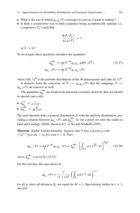
In many stochastic decision problems, a distinction has to be made between thescenario process (which contains decision-relevant values, such as prices, demands,and supplies) and the information which is available. Here is a simple example dueto Philippe Artzner.

Example A fair coin is tossed three times. Situation A: The payoff process ξ (A) is

ξ(A)1 = 0; ξ

(A)2 = 0;

ξ(A)3 =

{1 if heads is shown at least two times,0 otherwise.

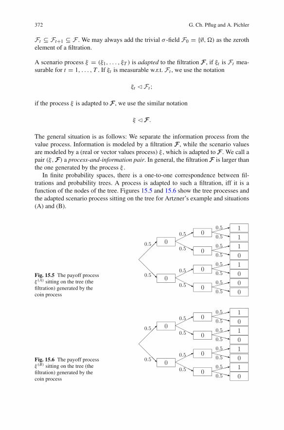
We compare this process to another payoff process (situation B)

ξ(B)1 = 0, ξ

(B)2 = 0,

ξ(B)3 =

{1 if heads is shown at least the last throw,0 otherwise.

The available information is relevant: It makes a difference, whether we mayobserve the coin tossing process or not. Suppose that the process is observable.Then, after the second throw, we know the final payoff, if two times the same sideappeared. Thus our information is complete although the experiment has not endedyet. Only in case that two different sides appeared, we have to wait until the lastthrow to get the final information.

Mathematically, the information process is described by a filtration.

Definition 3.4 Let (Ω,F , P) be probability space. A filtration FF on this probabilityspace is an increasing sequence of σ -fields FF = (F1, . . . ,FT ) where for all t ,


Ft ⊆ Ft+1 ⊆ F . We may always add the trivial σ -field F0 = {∅,�) as the zerothelement of a filtration.

A scenario process ξ = (ξ1, . . . , ξT ) is adapted to the filtration FF , if ξt is Ft mea-surable for t = 1, . . . , T . If ξt is measurable w.r.t. Ft , we use the notation

ξt � Ft ;

if the process ξ is adapted to FF , we use the similar notation

ξ � FF .

The general situation is as follows: We separate the information process from thevalue process. Information is modeled by a filtration FF , while the scenario valuesare modeled by a (real or vector values process) ξ , which is adapted to FF . We call apair (ξ,FF) a process-and-information pair. In general, the filtration FF is larger thanthe one generated by the process ξ .

In finite probability spaces, there is a one-to-one correspondence between fil-trations and probability trees. A process is adapted to such a filtration, iff it is afunction of the nodes of the tree. Figures 15.5 and 15.6 show the tree processes andthe adapted scenario process sitting on the tree for Artzner’s example and situations(A) and (B).

Fig. 15.5 The payoff processξ (A) sitting on the tree (thefiltration) generated by thecoin process

Fig. 15.6 The payoff processξ (B) sitting on the tree (thefiltration) generated by thecoin process


15.4.2.1 Tree Processes

Definition 3.5 A stochastic process ν = (ν1, . . . , νT ) is called a tree process, ifσ(ν1), σ(ν2), . . . , σ(νT ) is a filtration. A tree process is characterized by the prop-erty that the conditional distribution of ν1, . . . , νt given νt+1 is degenerated, i.e.,concentrated on a point. Notice that any stochastic process η = (η1, . . . , ηT ) can betransformed into a tree process by considering its history process

ν1 = η1,

ν2 = (η1, η2),

...

νT = (η1, . . . , ηT ).

Let (νt ) be a tree process and let FF = σ(ν). It is well known that any process ξadapted to FF can be written as ξt = ft (νt ) for some measurable function ft . Thus astochastic program may be formulated using the tree process ν and the functions ft .

Let ν be a tree process according to Definition 3.5. We assume throughout thatthe state spaces of all tree processes are Polish. In this case, the joint distribution Pof ν1, . . . , νT can be factorized into the chain of conditional distributions, which aregiven as transition kernels, that is

P1(A) = P{ν1 ∈ A},P2(A|u) = P{ν2 ∈ A|ν1 = u},

...

Pt (A|u1, . . . , ut−1) = P{νt ∈ A|ν1 = u1, . . . , νt−1 = ut−1}.

Definition 3.6 (Equivalence of tree processes) Let ν resp. ν two tree processes,which are defined on possibly different probability spaces (�,F , P) resp.(Ω, F , P). Let P1, P2, . . . , PT resp. P1, P2, . . . , PT be the pertaining chain ofconditional distributions. The two tree processes are equivalent, if the follow-ing properties hold: There are bijective functions k1, . . . , kT mapping the statespaces of ν to the state spaces of ν, such that the two processes ν1, . . . , νT andk−1

1 (ν1), . . . , k−1T (νT ) coincide in distribution.

Notice that for tree processes defined on the same probability space, one coulddefine equivalence simply as νt = kt (νt ) a.s. The value of Definition 3.6 is that itextends to tree processes on different probability spaces.

Definition 3.7 (Equivalence of scenario process-and-information pairs) Let (ξ, ν)be a scenario process-and-information pair, consisting of a scenario process ξ and atree process, such that ξ � σ(ν). Since ξ � σ(ν), there are measurable functions ft

such that

ξt = ft (νt ), t = 1, . . . T .


Two pairs (ξ, ν) and (ξ , ν) are called equivalent, if ν and ν are equivalent in thesense of Definition 3.6 with equivalence mappings kt such that

ξt = ft (k−1t (ξt )) a.s.

We agree that equivalent process-and-information pairs will be treated as equal.Notice that by drawing a finite tree with some values sitting on its nodes we auto-matically mean an equivalence class of process-and-information pairs.

If two stochastic optimization problems are defined in the same way, but usingequivalent process-and-information pairs, then they have equivalent solutions. It iseasy to see that an optimal solution of the first problem can be transformed into anoptimal solution of the second problem via the equivalence functions kt .

Figures 15.7 and 15.8 illustrate the concept of equivalence. The reader is invitedto find the equivalence functions kt in this example.

15.4.2.2 Distances Between Filtrations

In order to measure the distances between two discretizations on the same proba-bility space one could first measure the distance of the respective filtrations. This

Fig. 15.7 Artzner’s example: The tree process is coded by the history of the coin throws (H =head,T = tail), the payoffs are functions of the tree process

Fig. 15.8 A process-and-information pair which is equivalent to Artzner’s example in Fig. 15.4.The coding of the tree process is just by subsequent letters


concept of filtration distance for scenario generation has been developed by Heitschand Roemisch (2003) and Heitsch et al. (2006).

Let (Ω, F , P) be a probability space and let F and F be two sub-sigma algebrasof F . Then the Kudo distance between F and F is defined as

D(F , F) = max(sup{‖1lA−E(1lA|F)‖p : A ∈ F}, sup{‖1lB−E(1lB |F)‖p : A ∈ F}).(15.35)

The most important case is the distance between a sigma algebra and a sub-sigmaalgebra of it: If F ⊆ F , then (15.35) reduces to

D(F , F) = sup{‖1lA − E(1lA|F)‖p : A ∈ F}. (15.36)

If FF = (F1,F2, . . . ) is an infinite filtration, one may ask, whether this filtrationconverges to a limit, i.e., whether there is a F∞, such that

D(Ft ,F∞)→ 0 for t →∞.

If F∞ is the smallest σ -field, which contains all Ft , then D(Ft ,F∞) → 0.However, the following example shows that not every discrete increasing filtrationconverges to the Borel σ -field.

Example Let F be the Borel-sigma algebra on [0,1) and let Fn be the sigma alge-

bra generated by the sets[

k2n ,

k+12n

), k = 0, . . . , 2n − 1. Moreover, let An =⋃2n−1

k=0

[k2n ,

2k+12n+1

). Then E(1lAn |Fn) = 1

2 and ‖1lAn − E(1lAn |Fn)‖p = 1/2 for

all n. While one has the intuitive feeling that Fn approaches F , the distance isalways 1/2.

15.4.3 Nested Distributions

We define a nested distribution as the distribution of a process-and-information pair,which is invariant w.r.t. to equivalence. In the finite case, the nested distribution isthe distribution of the scenario tree or better of the class of equivalent scenario trees.

Let d be a metric on RM , which makes it a complete separable metric space and let

P1(RM , d) be the family of all Borel probability measures P on (RM , d) such that

∫d(u, u0) dP(u) <∞ (15.37)

for some u0 ∈ RM .

For defining the nested distribution of a scenario process (ξ1, . . . , ξT )with valuesin R

M , we define the following spaces in a recursive way:

�1 := RM ,


with distance dl1(u, v) = d(u, v):

�2 := RM × P1(�1)

with distance dl2((u, P), (u, Q)) := d(u, v)+ dKA(P, Q; dl1):

�3 := RM × P1(�2) = (RM × P1(R

M × P1(RM )))

with distance dl3((u,P), (v,Q)) := d(u, v) + dKA(P,Q; dl2). This construction isiterated until

�T = RM × P1(�T−1)

with distance dlT ((u,P), (v,Q)) := d(u, v)+ dKA(P,Q; dlT−1).

Definition 3.8 (Nested distribution) A Borel probability distribution P with finitefirst moments on �T is called a nested distribution of depth T ; the distance dlT iscalled the nested distance (Pflug 2009).

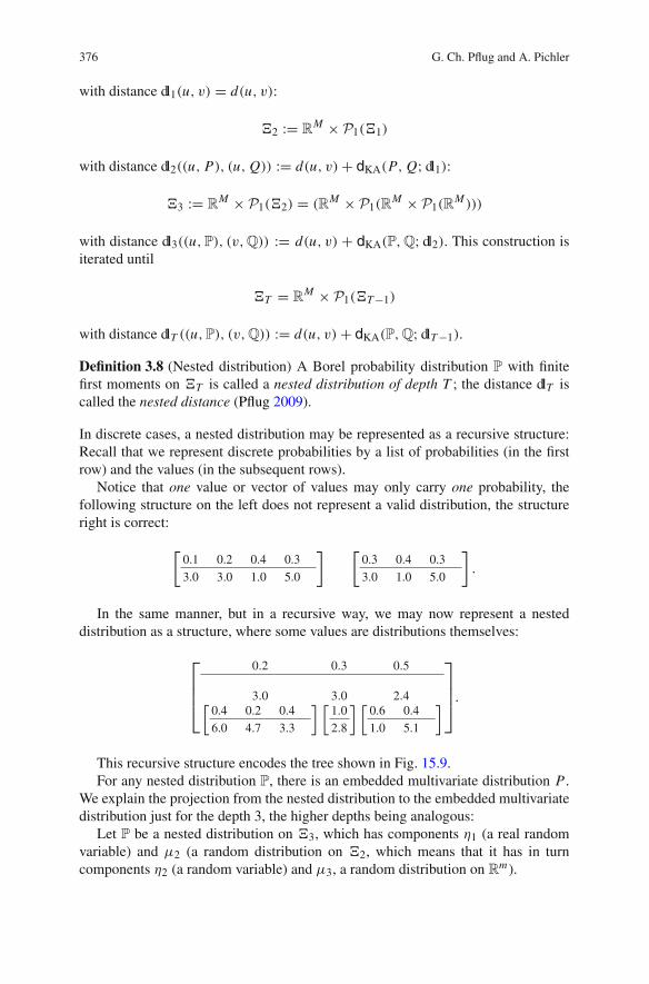
In discrete cases, a nested distribution may be represented as a recursive structure:Recall that we represent discrete probabilities by a list of probabilities (in the firstrow) and the values (in the subsequent rows).

Notice that one value or vector of values may only carry one probability, thefollowing structure on the left does not represent a valid distribution, the structureright is correct:

[0.1 0.2 0.4 0.3

3.0 3.0 1.0 5.0

] [0.3 0.4 0.3

3.0 1.0 5.0

].

In the same manner, but in a recursive way, we may now represent a nesteddistribution as a structure, where some values are distributions themselves:

⎡⎢⎢⎣

0.2 0.3 0.5

3.0 3.0 2.4[0.4 0.2 0.4

6.0 4.7 3.3

] [1.0

2.8

] [0.6 0.4

1.0 5.1

]

⎤⎥⎥⎦.

This recursive structure encodes the tree shown in Fig. 15.9.For any nested distribution P, there is an embedded multivariate distribution P .

We explain the projection from the nested distribution to the embedded multivariatedistribution just for the depth 3, the higher depths being analogous:

Let P be a nested distribution on �3, which has components η1 (a real randomvariable) and μ2 (a random distribution on �2, which means that it has in turncomponents η2 (a random variable) and μ3, a random distribution on R

m).


Fig. 15.9 Example tree

Then the pertaining multivariate distribution on Rm × R

m × Rm is given by

P(A1 × A2 × A3) = EP[1l{η1∈A1}Eμ2(1l{η2∈A2}μ2(A3))]

for A1, A2, A2 Borel sets in Rm .

The mapping from the nested distribution to the embedded distribution is notinjective: There may be many different nested distributions which all have the sameembedded distribution, see Artzner’s example: ξ (A) and ξ (B) in Figs. 15.5 and 15.6have different nested distributions, but the same embedded distributions. Here isanother example:

Example Consider again the process-and-information pair (the tree) of Fig. 15.9.The embedded multivariate but non-nested distribution of the scenario process is

⎡⎣0.08 0.04 0.08 0.3 0.3 0.2

3.0 3.0 3.0 3.0 2.4 2.46.0 4.7 3.3 2.8 1.0 5.1

⎤⎦ .

Evidently, this multivariate distribution has lost the information about the nestedstructure. If one considers the filtration generated by the scenario process itself andforms the pertaining nested distribution, one gets

⎡⎢⎢⎢⎣

0.5 0.5

3.0 2.4[0.16 0.08 0.16 0.6

6.0 4.7 3.3 2.8

] [0.6 0.4

1.0 5.1

]⎤⎥⎥⎥⎦

since in this case the two nodes with value 3.0 have to be identified.

Lemma 3.9 Let (ξ, ν) be equivalent to (ξ , ν) in the sense of Definition 3.7. Thenboth pairs generate the same nested distribution.

For a proof see Pflug (2009).


15.4.3.1 Computing the Nested Distance

Recall that a nested distribution is the distribution of a process-and-information pair,which is invariant w.r.t. equivalence. In the finite case, the nested distribution is thedistribution of the scenario tree (or better of the class of equivalent scenario trees),which was defined in a recursive way.

To compute the nested distance of two discrete nested distributions, P and P say,corresponds to computing the distance of two tree processes ν and ν. We furtherelaborate the algorithmic approach here, which is inherent is the recursive definitionof nested distributions and the nested distance.

To this end recall first that the linear program (15.20) was defined so general,allowing to compute the distance of general objects whenever probabilities ps , pt ,and the cost matrix cs,t were specified – no further specifications of the samples zare needed. We shall exploit this fact; in the situation we describe here the sampleszs and zt represent nested distributions with finitely many states, or equivalentlyentire trees.

Consider the nodes in the corresponding tree: Any node is either a terminal node,or a node with children, or the root node of the respective tree. The following recur-sive treatment is in line with this structure:

• Recursion start (discrete nested distribution of depth 1) In this situation thenested distributions themselves are elements of the underlying space, P ∈ �T

(P ∈ �T resp.), for which we have that

dlT (P, P) = d(P, P)

according to the definition.In the notion of trees this situation corresponds to trees which consist of a singlenode only, which are terminal nodes (leaf nodes).

• Recursive step (discrete nested distribution of depth t > 1) In this situation thenested distribution may be dissected in

Pt =(

nt ,∑

s

ptsδzt+1

s

)and Pt =

(nt ,

∑s

ptsδzt+1

s

),

where zt+1s ∈ �t+1 and zt+1

s ∈ �t+1.We shall assume that dlt+1 is recursively available, thus define the matrix

cs,s := d(nt , nt )+ dlt+1

(zt+1

s , zt+1s

)

and apply the linear program (15.20) together with the probabilities p = (ps)sand p = ( ps)s , resulting with the distance dlt (Pt , Pt ).

In the notion of trees, again, nt and nt represent nodes with children. The chil-dren are given by the first components of zt+1

s (zt+1s , resp.); further notice that


(zt+1s )s are just all subtrees of nt , all this information is encoded in the nested

distribution Pt .• Recursive end (nested distribution of depth t = T ) The computation of the

distance has already been established in the recursion step.

Note, that the corresponding trees in this situation represent the entire tree processhere.

15.4.3.2 The Canonical Construction

Suppose that P and P are nested distributions of depth T . One may construct thepertaining tree processes in a canonical way: The canonical name of each node isthe nested distribution pertaining of the subtree, for which this node is the root. Twovaluated trees are equivalent, iff the respective canonical constructions are identical.

Example 3.10 Consider the following nested distribution:

Pε =

⎡⎢⎢⎢⎣

0.5 0.5

2 2+ E[1.0

3

] [1.0

1

]⎤⎥⎥⎥⎦ .

We construct a tree process such that the names of the nodes are the correspondingnested distributions of the subtrees:

The nested distance generates a much finer topology than the distance of the multi-variate distributions.

Example (see Heitsch et al. (2006)) Consider the nested distributions of Example3.10 and

P0 =

⎡⎢⎢⎢⎣

1.0

2[0.5 0.5

3 1

]⎤⎥⎥⎥⎦ .


Note that the pertaining multivariate distribution of Pε on R2 converges weakly to

the one of P0, if ε → 0. However, the nested distributions do not converge: Thenested distance is dl(Pε,P0) = 1+ ε for all ε.

Lemma 3.11 Let P be a nested distribution, P its multivariate distribution, which isdissected into the chain P = P1 ◦ P2 ◦ · · · ◦ PT of conditional distributions. If P hasthe (K2, . . . , KT )-Lipschitz property (see Definition 3.2), then

dl(P, P) ≤T∑

t=1

d1(Pt , Pt )

T+1∏s=t+1

(Ks + 1).

For a proof see Pflug (2009).

Theorem 3.12 Let P resp. P be two nested distributions and let P resp. P be thepertaining multi-period distributions. Then

d1(P, P) ≤ dl(P, P).

Thus the mapping, which maps the nested distribution to the embedded multi-perioddistribution, is Lipschitz(1). The topologies generated by the two distances are notthe same: The two trees in Figs. 15.5 resp. 15.6 are at multivariate Kantorovichdistance 0, but their nested distance is dl = 0.25.

Proof To find the Kantorovich distance between P and P one has to find a jointdistribution for two random vectors ξ and ξ such that the marginals are P resp. P .Among all these joint distributions, the minimum of d(ξ1, ξt ) + · · · + d(ξT , ξT )

equals d(P, P). The nested distance appears in a similar manner; the only differ-ence is that for the joint distribution also the conditional marginals should be equalto those of P resp. P. Therefore, the admissible joint distributions for the nesteddistance are subsets of the admissible joint distributions for the distance between Pand P and this implies the assertion. !"Remark The advantage of the nested distance is that topologically different sce-nario trees with completely different values can be compared and their distance canbe calculated. Consider the example of Fig. 15.10. The conditional probabilitiesP(·|u) and Q(·|v) are incomparable, since no values of u coincide with values ofv. Moreover, the Lipschitz condition of Definition 3.2 does not make sense for treesand therefore Theorem 3.1 is not applicable. However, the nested distance is welldefined for two trees.

By calculation, we find the nested distance dl = 1.217.

Example Here is an example of the nested distance between a continuous processand a scenario tree process. Let P be the following continuous nested distribution:ξ1 ∼ N (0, 1) and ξ2|ξ1 ∼ N (ξ1, 1). Let P be the discrete nested distribution

⎡⎢⎣

0.30345 0.3931 0.30345

−1.029 0.0 1.029[0.30345 0.3931 0.30345

−2.058 −1.029 0.0

] [0.30345 0.3931 0.30345

−1.029 0.0 1.029

] [0.30345 0.3931 0.30345

0.0 1.029 2.058

]⎤⎥⎦


Fig. 15.10 Two valuated trees

Then the nested distance is d(P, P) = 0.8215, which we found by numerical dis-tance calculation.

15.5 Scenario Tree Construction and Reduction

Suppose that a scenario process (ξt ) has been estimated. In this section, we describehow to construct a scenario tree out of it. We begin with considering the case, wherethe information is the one which is generated by the scenario process and the methodis based on the conditional probabilities. Later, we present the case where a tree pro-cess representing the information and a scenario process sitting on the tree processhas been estimated.

15.5.1 Methods Based on the Conditional Distance

The most widespread method to construct scenario trees is to construct them recur-sively from root to leaves. The discretization for the first stage is done as describedin Section 15.2. Suppose a chosen value for the first stage is x . Then the referenceprocess ξt is conditioned to the set {ω : |ξ1 − x | ≤ ε}, where ε is chosen in such away that enough trajectories are contained in this set. The successor nodes of x arethen chosen as if x were the root and the conditional process were the total process.

The original distributions may either be continuous (e.g., estimated distributions)or more commonly discrete (e.g., simulated with some random generation mecha-nism which provides some advantages for practical usage). Different solution tech-niques for continuous as well as discrete approximation have been outlined in Pflug(2001) and Hochreiter and Pflug (2007).


Example The typical algorithm for finding scenario trees based on the Kantorovichdistance can be illustrated by the following pictures.

Step 1. Estimate the probability model and simulate future trajectories

t = 0 t = 1 t = 2 t = 340

60

80

100

120

140

160

180

Step 2. Approximate the data in the first stage by minimal Kantorovich distance

t = 0 t = 1 t = 2 t = 340

60

80

100

120

140

160

180


Step 3. For the subsequent stages, use the paths which are close to itspredecessor ...

t = 0 t = 1 t = 2 t = 340

60

80

100

120

140

160

180

Step 4. .. and iterate this step through the whole tree.

t = 0 t = 1 t = 2 t = 360

70

80

90

100

110

120

130

140

15.5.2 Methods Based on the Nested Distance

The general scenario tree problem is as follows:

15.5.2.1 The Scenario Tree Problem

Given a nested distribution P of depth T , find a valuated tree (with nested distance P)with at most S nodes such that the distance dl(P, P) is minimal.


Unfortunately, this problem is such complex, that is, it is impossible to be solvedfor medium tree sizes. Therefore, some heuristic approximations are needed. Apossible method is a stepwise and greedy reduction of a given tree. Two subtreesof the tree may be collapsed, if they are close in terms of the nested distance. Hereis an example:

Example The three subtrees of level 2 of the tree in Fig. 15.9. We calculated theirnested distances as follows:

dl

⎛⎜⎝⎡⎢⎣

1.0

2.4[0.4 0.6

5.1 1.0

]⎤⎥⎦ ,

⎡⎢⎣

1.0

3.0[1.0

2.8

]⎤⎥⎦⎞⎟⎠ = 2.6,

dl

⎛⎜⎝⎡⎢⎣

1.0

2.4[0.4 0.6

5.1 1.0

]⎤⎥⎦ ,

⎡⎢⎣

1.0

3.0[0.4 0.2 0.4

3.3 4.7 6.0

]⎤⎥⎦⎞⎟⎠ = 2.62,

dl

⎛⎜⎝⎡⎢⎣

1.0

2.4[0.4 0.6

5.1 1.0

]⎤⎥⎦ ,

⎡⎢⎣

1.0

3.0[0.4 0.2 0.4

3.3 4.7 6.0

]⎤⎥⎦⎞⎟⎠ = 1.86.

To calculate a nested distance, we have to solve∑T

t=1 #(Nt ) ·#(Nt ) linear optimiza-tion problems, where #(Nt ) is the number of nodes at stage t .

Example For the valued trees of Fig. 15.11we get the following distances:

dl(P(1),P(2)) = 3.90; d(P(1), P(2)) = 3.48,

dl(P(1),P(3)) = 2.52; d(P(1), P(3)) = 1.77,

dl(P(2),P(3)) = 3.79; d(P(2), P(3)) = 3.44.

0 1 2 3−4−3−2−1

012345

0 1 2 3−4

−3

−2

−1

0

1

2

3

0 1 2 3−4−3−2−1

0123456

Fig. 15.11 Distances between nested distributions


Example Let P be the (nested) probability distribution of the pair ξ = (ξ1, ξ2) bedistributed according to a bivariate normal distribution

(ξ1ξ2

)= N

((00

),

(1 11 2

)).

Note that the distribution of (ξ1, ξ2) is the same as the distribution of (ζ1, ζ1 + ζ2),where ζi are independently standard normally distributed.

We know that the optimal approximation of a N (μ, σ 2) distribution in theKantorovich sense by a three-point distribution is

[0.30345 0.3931 0.30345

μ− 1.029σ μ μ+ 1.029σ

].

The distance is 0.3397 σ . Thus the optimal approximation to ξ1 is

[0.30345 0.3931 0.30345

−1.029 0.0 1.029

]

and the conditional distributions given these values are N (−1.029, 1), N (0, 1), andN (1.029, 1). Thus the optimal two-stage approximation is

P(1)=

⎡⎢⎢⎢⎢⎢⎣

0.30345 0.3931 0.30345

−1.029 0.0 1.029⎡⎣ 0.30345 0.3931 0.30345

−2.058 −1.029 0.0

⎤⎦

⎡⎣ 0.30345 0.3931 0.30345

−1.029 0.0 1.029

⎤⎦

⎡⎣ 0.30345 0.3931 0.30345

0.0 1.029 2.058

⎤⎦

⎤⎥⎥⎥⎥⎥⎦.

The nested distance is dl(P, P(1)) = 0.76.Figure 15.12 shows on the left the density of the considered normal model P and

on the right the discrete model P(1).

−2−1

01

23

−3−2

−10

12

3

0

0.05

0.1

0.15

−2−1

01

23

−3−2

−10

12

30

0.05

0.1

0.15

Fig. 15.12 Optimal two stage approximation


−2−1

01

23

−3

−2

−1

0

1

2

3

0

0.05

0.1

0.15

−2−1

01

23

−3

−2

−1

0

1

2

3

0

0.05

0.1

Fig. 15.13 Randomly sampled approximation

For comparison, we have also sampled nine random points from P. Let P(2) be the

empirical distribution of these nine points. Figure 15.13 shows on the right side therandomly sampled discrete model P

(2). The nested distance is dl(P, P(2)) = 1.12.

15.6 Summary

In this contribution we have outlined some funding components to get stochasticoptimization available for computational treatment. At first stage the quantizationof probability measures is studied, which is essential to capture the initial prob-lem from a computational perspective. Various distance concepts are available ingeneral, however, only a few of them insure that the quality of the solution of theapproximated problem is in line with the initial problem.

This concept then is extended to processes and trees. To quantify the qualityof an approximating process, the concept of a nested distance is introduced. Someexamples are given to illustrate this promising concept.

The collected ingredients give a directive, how to handle a stochastic optimiza-tion problem in general. Moreover – and this is at least as important – they allowto qualify solution statements of any optimization problem, which have stochasticelements incorporated.

References

Z. Drezner and H.W. Hamacher. Facility Location: Applications and Theory. Springer, New York,NY, 2002.

J. Dupacova. Stability and sensitivity analysis for stochastic programming. Annals of OperationsResearch, 27:115–142, 1990.

Richard Durrett. Probability: Theory and Examples. Duxbury Press, Belmont, CA, second edition,1996.

A. Gibbs and F.E. Su. On choosing and bounding probability metrics. International StatisticalReview, 70(3):419–435, 2002.

S. Graf and H. Luschgy. Foundations of Quantization for Probability Distributions. Lecture Notesin Math. 1730. Springer, Berlin, 2000.


H. Heitsch and W. Roemisch. Scenario reduction algorithms in stochastic programming. Compu-tational Optimization and Applications, 24:187–206, 2003.

H. Heitsch, W. Roemisch, and C. Strugarek. Stability of multistage stochastic programs. SIAMJournal on Optimization, 17:511–525, 2006.

C.C. Heyde. On a property of the lognormal distribution. Journal of Royal Statistical SocietySeries B, 25(2):392–393, 1963.

R. Hochreiter and G. Ch. Pflug. Financial scenario generation for stochastic multi-stage decisionprocesses as facility location problems. Annals of Operation Research, 152(1):257–272, 2007.

K. Hoyland and S.W. Wallace. Generating scenario trees for multistage decision problems. Man-agement Science, 47:295–307, 2001.

S. Na and D. Neuhoff. Bennett’s integral for vector quantizers. IEEE Transactions on InformationTheory, 41(4):886–900, 1995.

H. Niederreiter. Random Number Generation and Quasi-Monte Carlo Methods, volume 23.CBMS-NSF Regional Conference Series in Applied Math., Soc. Industr. Applied Math.,Philadelphia, PA, 1992.

T. Pennanen. Epi-convergent discretizations of multistage stochastic programs via integrationquadratures. Mathematical Programming, 116:461–479, 2009.

G. Ch. Pflug. Scenario tree generation for multiperiod financial optimization by optimal discretiza-tion. Mathematical Programming, Series B, 89:251–257, 2001.

G. Ch. Pflug. Version-independence and nested distributions in multistage stochastic optimization.SIAM Journal on Optimization, 20(3):1406–1420, 2009.

S.T. Rachev and W. Roemisch. Quantitative stability in stochastic programming: The method ofprobability metrics. Mathematics of Operations Research, 27(4):792–818, 2002.

S.T. Rachev. Probability Metrics and the Stability of Stochastic Models. Wiley, New York, NY,1991.

S.S. Vallander. Calculation of the Wasserstein distance between probability distributions on theline. Theor. Prob. Appl., 18:784–786, 1973.

C. Villani. Optimal Transport. Springer, Berlin, Heidelberg, 2008.A. Weber. Theory of the Location of Industries. The University of Chicago Press, Chicago, IL

1929.

Chapter15 Approximations for Probability Distributions and ...€¦ · Chapter15 Approximations for...

Documents

Transcript of Chapter15 Approximations for Probability Distributions and ...€¦ · Chapter15 Approximations for...