Chapter XI A Method of Estimation for Magnetic Resonance...

��

Chapter XIA Method of Estimation for

Magnetic Resonance Spectroscopy Using

Complex-Valued Neural Networks

Naoyuki MoritaKochi Gakuen College, Japan

Copyright © 2009, IGI Global, distributing in print or electronic forms without written permission of IGI Global is prohibited.

INTrODUCTION

Magnetic resonance spectroscopy (MRS) is used to determine the quantity of metabolites, such as creatine phosphate (PCr) and adenocine triphosphate (ATP), in the living body by collecting their nuclear magnetic resonance (NMR) spectra. In the field of MRS, the frequency spectrum of metabolites is usually obtained by applying the fast Fourier transform (FFT) (Cooley & Tukey, 1965) to the NMR signal collected from the living

ABSTrACT The author proposes an automatic estimation method for nuclear magnetic resonance (NMR) spectra of the metabolites in the living body by magnetic resonance spectroscopy (MRS) without human intervention or complicated calculations. In the method, the problem of NMR spectrum estimation is transformed into the estimation of the parameters of a mathematical model of the NMR signal. To estimate these parameters, Morita designed a com-plex-valued Hopfield neural network, noting that NMR signals are essentially complex-valued. In addition, we devised a technique called “sequential extension of section (SES)” that takes into account the decay state of the NMR signal. Morita evaluated the performance of his method using simulations and shows that the estimation precision on the spectrum improves when SES is used in combination the neural network, and that SES has an ability to avoid the local minimum solution on Hopfield neural networks.

��

A Method of Estimation for Magnetic Resonance Spectroscopy Using Complex-Valued Neural Networks

body. Then, quantification of the metabolites is carried out by estimating the area under each spectral peak using a curve fitting procedure (Maddams, 1980; Mierisová & Ala-Korpel, 2001; Sijens et al., 1998), as described in the BACKGROUND section. However, this method is not suitable for processing large quantities of data because human intervention is necessary. In this chapter, an automatic spectral estimation method, which we developed in order to process large quantities of data without human intervention, is presented.

This chapter is organized as follows: BACKGROUND reviews MRS and some conventional estimation methods of NMR spectra, and briefly outlines our method. MATHEMATICAL MODEL OF THE NMR SIGNAL AND ESTIMATION OF SPECTRA first, gives an overview of NMR phenomenon and NMR signal, next, presents a mathematical model of the NMR signal; and finally, describes our approach to spectral estimation. DESIGN OF A COMPLEX-VALUED HOPFIELD NEURAL NETWORK AS A SPECTRAL ESTIMATIOR describes the design of our complex-valued Hopfield neural network. SEQUENTIAL EXTENSION OF SECTION (SES) explains the concept of SES. For performance evaluation of our method, simulations were carried out using sample signals that imitate an actual NMR signal, and the results of those simulations are given in SIMULATIONS. The results are evaluated and discussed in DISCUSSION. Finally, we give some conclusions and future research directions.

BACKGrOUND

Magnetic resonance imaging (MRI) systems, which produce medical images using the nuclear magnetic resonance (NMR) phenomenon, have recently become popular. Additional technological innovations, such as high-speed imaging technologies (Feinberg & Oshio, 1991; Henning, Nauerth, & Fnedburg, 1986; Mansfield, 1977; Melki, Mulkern, Panych, & Joles, 1991; Meyer, Hu, Nishimura, & Macovski, 1992) and imaging of brain function using functional MRI (Belliveau et al., 1991; Kwong et al., 1992; Ogawa, Lee, Nayak, & Glynn, 1990), are also rapidly progressing. Currently, the above-mentioned imaging technologies mainly take advantage of the NMR phenomena of protons. The atomic nuclei used for analyzing metabolism in the living body include proton, phosphorus-31, carbon-13, fluorine-19 and sodium-22. Phosphorus-31 NMR spectroscopy has been widely used for measurement of the living body, because it is able to track the metabolism of energy.

NMR was originally developed and used in the field of analytical chemistry. In that field, NMR spectra are used to analyze the chemical structure of various materials. This is called NMR spectroscopy. In medical imaging, it is also possible to obtain NMR spectra. In this case, the technique is called magnetic resonance spectroscopy (MRS), and it can be used to collect the spectra of metabolites in organs such as the brain, heart, liver and muscle. The difference between NMR spectroscopy and MRS is that in MRS, we collect spectra from the living body in a relatively low magnetic field (usually, about 1.5 Tesla); in NMR spectroscopy, small chemical samples are measured in a high magnetic field.

In MRI systems, the Fourier transform is widely used as a standard tool to produce an image from the measured data and to obtain NMR spectra. In NMR spectroscopy, we can obtain a frequency spectrum by applying the fast Fourier transform (FFT) to the free induction decay (FID) that is observed as a result of the magnetic relaxation phenomenon (Derome, 1987). Here the FID is an NMR signal in the time domain and it is a time series, that is, it can be modeled as a set of sinusoids exponentially damping with time. When the FFT is applied to such a signal, the spectral peaks obtained are of the form called a Lorentz curve (Derome, 1987). If the signal is damped rapidly, the height of the spectral peaks will be decreased and the width of the peaks will increase. This is an inevitable result of applying FFT to FIDs. In addition, the resolution of the spectrum collected in a low magnetic field is much lower than a typical spectrum obtained by NMR spectroscopy. Thus, the spectra by MRS are quite different from those by NMR spectroscopy. That is, the spectral peaks obtained by MRS are spread out and the spectral distribution obtained is very different from the original distribution as shown in Figure 1. Thus, we can-not use a peak height to quantify a metabolite. Instead, we estimate the area under each peak using curve-fitting procedures (Figure 1(d): non-linear least square methods) (Maddams, 1980; Mierisová & Ala-Korpela, 2001; Sijens et al., 1998). However, existing curve-fitting procedures are inadequate for processing large quantities of data because they require human intervention. The aim of us is to devise a method that does not require such a human intervention.

��


We can consider two approaches to this problem: (1) automating the description of spectral peaks and the determination of the peak areas, and (2) using methods of estimation and quantification other than the Fourier transform. In the first approach, attempts at automatic quantification of NMR spectra using hierarchical neural networks have been reported (Ala-Korpela et al., 1997; Kaartinen et al., 1998). In this research, a three-layered network based on back propagation (Rumelhart, Hinton, & Williams, 1986) was employed to estimate spectra in the frequency domain. The fully-trained network had the ability to quantify unknown spectra automatically, and curve fitting procedures were not necessary. However, large amounts of training data were necessary to increase the precision of quantification. These methods quantify the spectra instead of performing the curve fitting procedures. In the second approach, the maximum entropy method (MEM), derived from the autoregressive (AR) model and the linear prediction (LP) method, and other similar methods have been studied widely (Haselgrove, Subramanian, Christen, & Leigh, 1988; van Huffel, Chen, Decanniere, & Hecke, 1994). These are parametric methods, that is, in these methods, a mathematical model of the signal is assumed and the parameters of that model are estimated from observed data. The spectrum can then be estimated from the model parameters. However, methods based on AR modeling require large amounts of calculation.

Our objective is to develop a method to estimate NMR spectra without human intervention or complicated calculations. For this, we took a parametric approach in which a neural network is used (Han & Biswas, 1997), and used Hopfield neural network (Hopfield, 1982, 1984), which does not have a learning process. It is possible

Figure 1. The effect of the Fourier transform for the spectral estimation in MRS:(a) The spectrum corresponding to the FID shown in Figure 1(b), (c) The spectrum obtained by applying the Fourier transform to Figure 1(b), (d) The curve-fitting procedure using the Lorentz function. The area of each Lorentz curve approximates the area of each spectral peak

(a) Original spectrum (b) FID

(c) Fourier Transform Spectrum (d) Curve-fitting procedure

��


to estimate the parameters using the ability of the neural network to find a local minimum solution or a minimum solution. In addition, we noted that NMR signals are essentially complex-valued and developed a method to estimate the spectrum using complex-valued Hopfield networks (Hirose, 1992a, 1992b; Zhou & Liu, 1993), in which the weights and thresholds for conventional networks are expanded to accommodate complex numbers. Both a hierarchical type (Benvenuto & Piazza, 1992; Georgiou & Koutsougeras, 1992; Nitta, 1991, 1997) and a recurrent type (Jankowski, Lozowski, & Zurada,1996; Nemoto & Kono, 1991) have been proposed as complex-valued neural networks. Furthermore, we have devised a technique that takes into account the decay state of the NMR signal, which we call “sequential extension of section” (SES), and have used it with the above-mentioned method.

MATHEMATICAL MODEL OF THE NMr SIGNAL AND ESTIMATION OF SPECTrA

NMR Background

If the number of neutrons plus the number of protons is odd, or if the number of neutrons and the number of the protons are both odd, nuclei possess a property called spin. In quantum mechanics, spin is represented by a spin magnetic quantum number. Spin can be visualized as a rotating motion of the nucleus. Since a nucleus is a charged particle, the spinning motion causes a magnetic moment in the direction of the spin axis as shown in Figure 2. Quantum mechanics tells us that a nucleus of spin I will have 2I+1 possible orientations. Considering a nucleus of spin ½, it will have two possible orientations.

We now consider a nucleus of spin ½ (such as proton, carbon-13 and phosphorus-31). In the absence of an externally applied magnetic field, the magnetic moments are randomly oriented, but when a field B0 is applied, they are constrained to adopt one of two orientations, denoted parallel and anti-parallel with respect to B0 (Figure 3). These two orientations correspond to the two energy levels: the lower and the higher, respectively. Nuclei with higher spin magnetic quantum number will adopt more than two orientations. The spin axes cannot be oriented exactly parallel (or anti-parallel) with the direction of B0, hence, they precess around B0 with a characteristic frequency as shown in Figure 4. The Larmor equation expresses the relationship between the strength of a magnetic field B0 and the precessional frequency (Larmor frequency) ω0 of an individual spin:

0 0B= ( : the gyromagnetic ratio of the nucleus). (1) When the nucleus is in a static magnetic field B0, the initial populations of the energy levels are determined

by thermodynamics, as described by the Boltzmann distribution. It means that the lower energy level will contain slightly more nuclei than the higher level. That is, let the numbers of spins adopting the parallel and anti-parallel be P1 and P2 respectively, we have P1 > P2.

At any given instant, the magnetic moments of nuclei can be represented as vectors, as shown in Figure 5(b). Every vector can be described by its components perpendicular to and parallel to B0. For a large enough number

Figure 2. A charged, spinning nucleus creates a magnetic moment which acts like a bar magnet (dipole)

��0


of spins, all the opposing components will cancel each other out. That is, individual components perpendicular to B0 will cancel, and a bulk magnetization vector (called the net magnetization M) will create in the direction of the B0 field, because of P1 > P2 (Figure 5(c)).

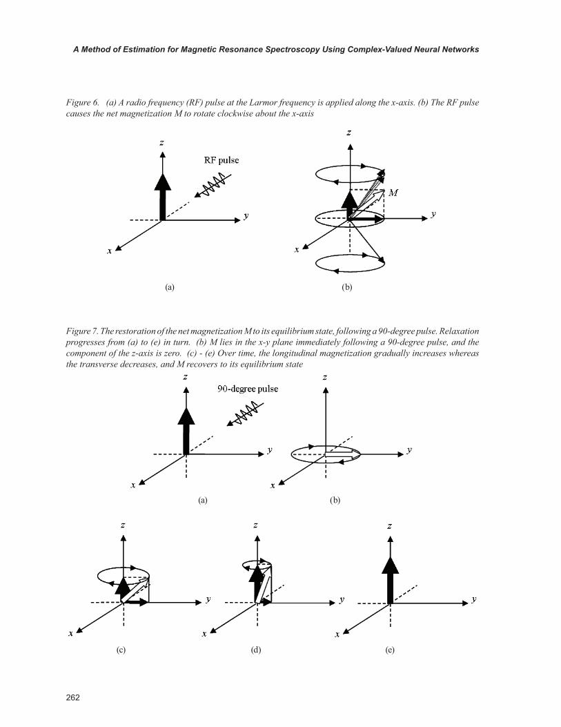
Suppose the direction of B0 is aligned with the z-axis of three-dimensional Euclidean space. The plane perpendicular to B0 contains the x and y-axes. In order to observe an NMR signal from nuclei, we must apply a radio frequency (RF) pulse at the Larmor frequency (the resonance frequency) of the nuclei. When the RF pulse is irradiated along the x-axis as shown in Figure 6(a), this pulse causes nuclear spins to swap between parallel

Figure 3. (a) Nuclei in the absence of an externally applied magnetic field. (b) An external magnetic field B0 is applied which cause the nuclei to align themselves in one of two orientations with respect to B0 (denoted parallel and anti-parallel)

(a) (b)

Figure 4. (a) In the presence of an externally applied magnetic field B0, nuclei are constrained to adopt one of two orientations with respect to B0. Since the nuclei possess spin, these orientations are not exactly at 0 and 180 degrees to B0. θ is the angle between of the applied field and the axis of nuclear rotation. (b) A magnetic moment precessing around B0

(a) (b)

��


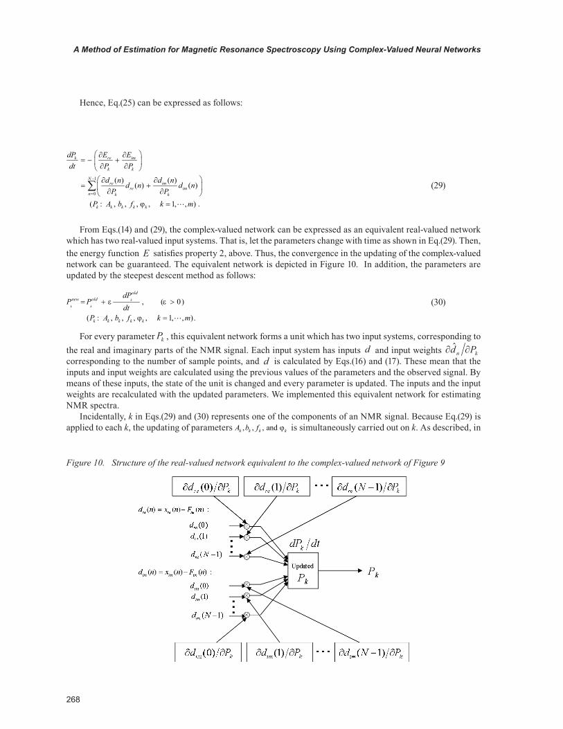
an anti-parallel states, and every phase of spins becomes in-phase along the direction of y-axis. As a result, the population of spins will change, and the net magnetization M will rotate clockwise about the x-axis (Figure 6(b)). Especially, the RF pulse that rotates M into the x-y plane is called “90-degree pulse” (Figure 7(a)(b)).

Following termination of an RF pulse, the restoration of M to its equilibrium state (the direction of the z-axis) known as relaxation begins. Figure 7(a-e) describes the relaxation following a 90-degree pulse.

Let M0 be the amount of magnetization of equilibrium state before an RF pulse is irradiated. Let Mz be the z component of M at time t, following a 90-degree pulse at time t = 0. It can be shown that the process of equilibrium restoration is described by the equation:

1/0 (1 )t T

zM M e−= − . (2)

Where T1 is the longitudinal relaxation time. Let M0xy be the amount of transverse magnetization immediately following a 90-degree pulse.

Let Mxy be the amount of transverse magnetization at time t, following a 90-degree pulse at time t = 0. Following the RF pulse, the magnetic moments interact with each other causing a decrease in the transverse magnetization. It can be shown that

*2/

0t T

xy xyM M e−= ⋅ . (3)

Where *2T characterizes the dephasing due to both B0 inhomogeneity and true transverse relaxation, and it

is called the apparent transverse relaxation time. In order to obtain a true transverse relaxation time T2, we must use a pulse sequence such as the spin-echo method (Denome, 1987).

Every magnetization vector is precessing about the applied magnetic field B0. Therefore, the component in the x-y plane is inevitably precessing about the B0 axis. In addition, as described above, the magnetization in the x-y plane decays with time. Accordingly, the magnetization in the x-y plane rotates about the z-axis, and decays over time. If we place a receiver coil in the x-y plane, this rotating magnetization will induce an electromotive force in it. The signal induced in the receiver coil is termed a free induction decay (FID). An FID is an NMR signal. Figure 8 shows the phenomenon described here.

Figure 5. (a) A precessing nucleus. (b) Vector representations of the magnetic moments at any given instant. (c) A small net magnetization M is detectable in the direction of the B0

(a) (b) (c)

��


Figure 6. (a) A radio frequency (RF) pulse at the Larmor frequency is applied along the x-axis. (b) The RF pulse causes the net magnetization M to rotate clockwise about the x-axis

(a) (b)

Figure 7. The restoration of the net magnetization M to its equilibrium state, following a 90-degree pulse. Relaxation progresses from (a) to (e) in turn. (b) M lies in the x-y plane immediately following a 90-degree pulse, and the component of the z-axis is zero. (c) - (e) Over time, the longitudinal magnetization gradually increases whereas the transverse decreases, and M recovers to its equilibrium state

(c) (d) (e)

(a) (b)

��


Mathematical Model of the NMR Signal

An NMR signal (FID) with m components is modeled as follows:

1

ˆ exp( )exp[ (2 )], 0,1, , 1m

n k k k kk

x A b n j f n n N=

= − + = −∑ , (4)

where )1,,1,0(ˆ −= Nnxn denotes the observed signal, which is complex-valued, n denotes the sample point

on the time axis and the sample period T is taken for T=1 to simplify the expression of Eq. (4). , , , andk k k kA b f are real number and denote the spectral composition, damping factor, rotation frequency and phase in the rotation,

respectively, of each metabolite. m is the number of the metabolites composing a spectrum, and 1−=j .

NMR Spectra

The position of each peak appearing in a NMR spectrum depends on its offset frequencies (chemical shifts) from the resonance frequency of a target nucleus under a specified static magnetic field (Derome, 1987). These offset frequencies are fk (k=1,…,m).

In a common pulse method, each peak possesses the offset phase expressed by a linear function of its offset frequencies f , as follows (Derome, 1987):

( )f f= + ⋅ . (5)

Where, α is called the zero-dimensional term of phase correction, and is a common phase error influencing every peak. β is called the one-dimensional term of phase correction, and is a phase error that is dependent on the offset frequencies, or more specifically, the positions of each peak.

Thus, in NMR spectra, the position of each peak and the scale of their offset phase are determined by the measurement condition used. Because of this fact, it is possible to make a rough prediction of the position of each peak of a NMR spectrum under specified measurement conditions. This positional can be used as a constrained condition when estimating unknown parameters using our neural network. In addition, because the relationship between a specified static magnetic field and the apparent transverse relaxation time T2

* of a target nucleus are known in MRS (Haselgrove, Subramanian, Christen, & Leigh, 1988), it is possible to determine the rough scale

Figure 8. (a) The transverse magnetization in the x-y plane rotates about the z-axis. The measurement of the component of the transverse magnetization in the x-y plane decays over time. An alternating signal shown in Figure (b) is induced in the receiver coil

(a) (b)

��


of T2* for a target nucleus when the strength of the static magnetic field is known. This information regarding T2

*

can also be used as a constraint condition. That is, it can be used for the estimation of bk.

Estimation of NMR Spectra

The following approach is used in our method of parametric spectral estimation.

1. A mathematical model of the NMR signal is given, as described above.2. Adequate values are supplied as initial values of the parameters , , , andk k k kA b f , and an NMR signal is

simulated. 3. The sum of the squares of the difference, at each sample point, between the simulated signal and the actual

observed signal is calculated.4. The parameters are varied to give optimum estimates for the observed signal by minimizing the error sum

of squares.

DESIGN OF A COMPLEX-VALUED HOPFIELD NEUrAL NETWOrK AS A SPECTrAL ESTIMATOr

Energy Function on the Complex-Valued Neural Network

For the estimation of NMR spectra, the error sum of squares of the parameter estimation problem is defined as the energy function of a Hopfield network. This means that the parameter estimation problem is converted to an optimization problem for the Hopfield network. The energy function is defined as

21

0 1

1 ˆ exp( )exp{ (2 )}2

N m

n k k k kn k

E x A b n j f n−

= =

= − − − +∑ ∑ , (6)

where, as in Eq.(4), n denotes the sample point on the time axis and nx̂ denotes the complex-valued observed signal at n .

The energy function E of complex-valued neural networks should have the following properties (Hashimoto, Kuroe, & Mori, 1999; Kuroe, Hashimoto, & Mori, 2002):

1. A function that relates the state nx̂ denoted by a complex number to a real-valued number.2. To converge on the optimum solution, it is always necessary to satisfy the following condition in the dynamic

updating of the Hopfield network:

( ) 0dEdt

⋅≤ , (7)

where t means the time on updating the network.

The energy function defined by Eq.(6) satisfies property 1. In Eq.(6), if

1

ˆ ˆ exp( )exp{ (2 )}m

n n k k k kk

d x A b n j f n=

= − − +∑ , (8)

then the energy function can be expressed as

1 12*

0 0

1 1ˆ ˆ ˆ2 2

(* : denotes the complex conjugate) .

N N

n n nn n

E d d d− −

= =

= − = −∑ ∑ (9)

��


From Eq.(6), when the parameters , , , andk k k kA b f in Eq.(4) are replaced by kP , the time variation of the above energy function can be expressed as

1, ( : , , , , 1, , ).

k

mk

k k k k kk P k

dPdE E P A b f k mdt P dt=

∂= =

∂∑∑

(10)

Here, suppose that

k

k

dP Edt P ⋅

∂= −

∂ (11)

Then,

2

10

k

m

k P k

dE Edt P=

∂= − ≤ ∂

∑∑ (12)

will hold, and property 2 is satisfied. Hence, the convergence in the dynamic updating of the complex-valued neural network is guaranteed.

Design of the Network

From Eq.(9), the variation of the energy function with respect to the variation of the parameters is as follows:

*1*

0

ˆ ˆ1 ˆ ˆ .2

Nn n

n nnk k k

d dE d dP P P

−

=

∂ ∂∂= − + ∂ ∂ ∂

∑ (13)

Then, by Eq.(11), we have

*1*

0

ˆ ˆ1 ˆ ˆ .2

k

k

Nn n

n nn k k

dP Edt P

d dd d

P P

−

=

∂= −

∂

∂ ∂= + ∂ ∂

∑

(14)

Eq. (14) expresses the time variation of the parameters kP , that is, the updating of the parameters. If we sup-

pose that *ˆnd and nd̂ on the right-hand side of the equation are the inputs to the complex-valued Hopfield neural

network and kn Pd ∂∂ ˆ and kn Pd ∂∂ *ˆ are the input weights in the network, a complex-valued network can be designed. The inputs and the input weights are then calculated by Eq.(8). In this network, two complex-valued input systems conjugated to each other are input to the network. The updating of the parameters is then carried out by complex calculation. However, because the two terms on the right-hand side of Eq.(14) are complex conjugates to each other, the left-hand side is a real number. The structure of the complex-valued network is depicted in Figure 9, where the coefficient 1/2 in Eq.(14) is omitted. Two complex-valued input systems conjugated to each other are input to one unit, and the updating of the parameters is carried out by complex-valued calculation.

Here, Eq. (8) can be decomposed into a real part )(ndre and an imaginary part )(ndim :

ˆ ( ) ( )n re imd d n jd n= + . (15)

��


Suppose that the real and imaginary parts of nx̂ are denoted as xre(n) and xim(n), respectively. We then have

1

( ) ( ) exp( )cos(2 ) ,m

re re k k k kk

d n x n A b n f n=

= − − +∑ (16)

1( ) ( ) exp( )sin(2 ) .

m

im im k k k kk

d n x n A b n f n=

= − − +∑ (17)

From these,

{ }{ }{ } { }

2*

2 2

ˆ ˆ ˆ (* : complex conjugate)

( ) ( ) ( ) ( )

( ) ( ) .

n n n

re im re im

re im

d d d

d n jd n d n jd n

d n d n

=

= + −

= + (18)

Then, Eq.(9) can be developed as follows:

1 2

0

1 ˆ ,2

N

n re imn

E d E E−

=

= − = +∑ (19)

{ }1

2

0

1 ( ) ,2

N

re ren

E d n−

=

= − ∑ (20)

{ }1

2

0

1 ( ) .2

N

im imn

E d n−

=

= − ∑ (21)

Figure 9. Structure of the complex-valued Hopfield network

��


From Eqs.(10) and (19), we obtain

1

1,

k

k

mk

k P k

re im

mre im k

k P k k

dPdE Edt P dt

dE dEdt dt

E E dPP P dt

=

=

∂=

∂

= +

∂ ∂= + ∂ ∂

∑∑

∑∑ (22)

where,

1,

mre re k

k k

dE E dPdt P dt=

∂=

∂∑ (23)

1

( : , , , ) .

mim im k

k k

k k k k k

dE E dPdt P dt

P A b f=

∂=

∂∑ (24)

Here, if we assume that

( : , , , , 1, , ) ,

k re im

k k

k k k k k

dP E Edt P P

P A b f k m

∂ ∂= − + ∂ ∂

=

(25)

we obtain the following:

2

10 .

k

mre im

k P k k

E EdEdt P P=

∂ ∂= − + ≤ ∂ ∂

∑∑

(26)

From Eqs.(20) and (21), we obtain

1

0

( )( ) ,

Nre re

renk k

E d nd n

P P

−

=

∂ ∂= −

∂ ∂∑ (27)

1

0

( )( ) .

Nim im

imnk k

E d nd n

P P

−

=

∂ ∂= −

∂ ∂∑ (28)

��


Hence, Eq.(25) can be expressed as follows:

1

0

( ) ( )( ) ( )

( : , , , , 1, , ) .

k re im

k k

Nre im

re imn k k

k k k k k

dP E Edt P P

d n d nd n d n

P PP A b f k m

−

=

∂ ∂= − + ∂ ∂

∂ ∂= + ∂ ∂

=

∑

(29)

From Eqs.(14) and (29), the complex-valued network can be expressed as an equivalent real-valued network which has two real-valued input systems. That is, let the parameters change with time as shown in Eq.(29). Then, the energy function E satisfies property 2, above. Thus, the convergence in the updating of the complex-valued network can be guaranteed. The equivalent network is depicted in Figure 10. In addition, the parameters are updated by the steepest descent method as follows:

, ( 0)

( : , , , , 1, , ).

k

k k

oldnew old

k k k k k

dPP P

dtP A b f k m

= + >

=

(30)

For every parameter kP , this equivalent network forms a unit which has two input systems, corresponding to the real and imaginary parts of the NMR signal. Each input system has inputs d and input weights kn Pd ∂∂ ˆ corresponding to the number of sample points, and d is calculated by Eqs.(16) and (17). These mean that the inputs and input weights are calculated using the previous values of the parameters and the observed signal. By means of these inputs, the state of the unit is changed and every parameter is updated. The inputs and the input weights are recalculated with the updated parameters. We implemented this equivalent network for estimating NMR spectra.

Incidentally, k in Eqs.(29) and (30) represents one of the components of an NMR signal. Because Eq.(29) is applied to each k, the updating of parameters , , , andk k k kA b f is simultaneously carried out on k. As described, in

Figure 10. Structure of the real-valued network equivalent to the complex-valued network of Figure 9

��


the network used in this chapter, the sequential updating of each unit, which is a feature of the Hopfield network, is transformed to sequential updating of every unit group , , , andk k k kA b f on k.

SEQUENTIAL EXTENSION OF SECTION (SES)

As expressed in Eq. (4), the NMR signal is a set of sinusoidal waves in which the spectral components Ak are exponentially damped with time n. We introduced the operation shown in Figure 11 so that our network would recognize the decay state more accurately. In the figure, the horizontal axis shows the sample points at time n, and the vertical axis shows the NMR signal. In this operation, first, appropriate values are assigned as initial values for each of the parameters. Then, our network operates on section A from time 0 (n = 0) to an adequate time )( 11 knk = . The parameter estimates are obtained when the network has equilibrated. Next, the network operates on section B from time 0 to an adequate time )( 212 kkk < , and the equilibrium values in section A are used as the initial values in section B. Thereafter, we extend the section in the same way, and finally, the network operates on the entire time interval corresponding to all sample points. This operation is equivalent to recogniz-ing the shape of the signal by gradually extending the observation section while taking into account the detailed aspects of the signal during its rapid variation.

For operating the SES, the length and number of above-mentioned sections naturally depend on the decay state of a target signal, and those values should be properly determined in objective and quantitative ways. However, because we did not find such a way, we applied the other one, as mentioned in “Sections Used for Sequential Extension of Section (SES) Method” of “SIMULATIONS”.

SIMULATIONS

Sample Signals

We simulated sample signals equivalent to NMR signals that consisted of 1024 data points on a spectrum with a bandwidth of 2000 Hz, which is equivalent to the range of about 58ppm on chemical shift, in order to deal with

Figure 11. Illustration of the sequential extension of section (SES) method

��0


every spectral peak of the atomic nucleus of phosphorus-31 in a static magnetic field of 2 Tesla. The three signals shown in Table 1 and Figs. 12-14 were used.

In Table 1, peaks 1 through 7 represent phosphomonoester (PME), inorganic phosphate (Pi), phosphodiester (PDE), creatine phosphate (PCr), γ-adenocine triphosphate (γ-ATP), α-ATP, and β-ATP, respectively.

Signals 1 and 3 are equivalent to the spectra of healthy cells with a normal energy metabolism. Pi is one of relatively-small spectral components in their signals. Signal 2 is equivalent to the spectrum of a cell that is approaching necrosis. In such cells, the metabolism of energy is decreased and Pi is large in comparison with other components, as shown in Table 1. This signal is analogous to a single-component spectral signal (a mono-tonic damped signal) compared with signal 1 and 3. Among these signals, only the spectral component Ak is different.

Implementation of the Network

We introduced some auxiliary operations that are necessary for stable implementation of our network.

Initial Values of the Parameters

The settings of the initial values of the parameters are shown in Table 2. For the amplitude Ak, the amplitudes of the real part and the imaginary part were compared; the larger was divided by 7, the number of signal compo-nents; and the result was used as the initial value for all seven components. For the initial values of the frequency fk and the damping coefficient bk of each metabolite, rough values are known for fk and bk under observation conditions, as described in “NMR Spectra” above. Therefore, the initial values were set close to their rough values. In addition, all of the initial phases were set to zero.

Updating of Units

In the steepest descent method in Eq.(30), two values, 10-5 and 10-6 were used as learning rate ε. By setting the upper limit of the number of the parameter updates to 50,000, we ensure that the units continue to be renewed until the energy function decreases. Then, the parameters can be updated while the energy function is decreasing and the number of renewals does not exceed the upper limit. By using these procedures, it is possible to operate the network in a stable condition. In addition, the following two conditions for stopping the network are set.

1. The updates of all parameters are terminated2. The energy function reaches an equilibrium point

Table 1. Parameters of sample signals

* : Relative values corresponding to the range from 1000 Hz to –1000 Hz around the resonance frequency. 0.0 is 1000 Hz, and 1.0 is –1000 Hz. ** : Values normalized to π.

Peak Metabolite fk* bk φ k**Ak

(1) (2) (3)

1 Phosphomonoester (PME) 0.368 0.05395 0.4774 0.726 0.7 0.996

2 Inorganic phosphate (Pi) 0.397 0.03379 0.3699 1.02 6.246 0.5

3 Phosphodiester (PDE) 0.435 0.05918 0.2296 2.1 1.8 2.1

4 Creatine phosphate (PCr) 0.485 0.03785 0.051 2.37 1.2 3.6

5 γ-adenocine triphosphate (γ-ATP) 0.526 0.04858 -0.1002 1.89 0.5 1.15

6 α-adenocine triphosphate (α-ATP) 0.616 0.05744 -0.4264 2.04 0.5 2.2

7 β-adenocine triphosphate (β-ATP) 0.763 0.04035 -0.9657 1.1 0.3 0.7

��


Figure 12. Signal 1 Figure 13. Signal 2

Figure 14. Signal 3

Table 2. Initial values of parameters

Peak Metabolite fk bk φk

Ak

(1) (2) (3)

1 Phosphomonoester (PME) 0.35 0.1 0.0 1.481595 1.502836 1.505209

2 Inorganic phosphate (Pi) 0.4 0.1 0.0 1.481595 1.502836 1.505209

3 Phosphodiester (PDE) 0.45 0.1 0.0 1.481595 1.502836 1.505209

4 Creatine phosphate (PCr) 0.5 0.1 0.0 1.481595 1.502836 1.505209

5 γ-adenocine triphosphate(γ-ATP) 0.55 0.1 0.0 1.481595 1.502836 1.505209

6 α-adenocine triphosphate(α-ATP) 0.6 0.1 0.0 1.481595 1.502836 1.505209

7 β-adenocine triphosphate (β-ATP) 0.75 0.1 0.0 1.481595 1.502836 1.505209

��


The criterion for condition 1 is a limit on the time variation of the parameter Pk: if0.01kdP dt ≤ , we set 0kdP dt = and terminate the updating of the parameter.

Regarding condition 2, we judge that the energy function has reached an equilibrium point when the energy function increases, or when the number of the updates exceeds the upper limit mentioned above. Theoretically, the network stops and an optimum solution is obtained when the above two conditions are satisfied simultaneously. However, because a monotonic decrease of the energy function is produced by the above-described operations, in practice, we forced the network to stop when either of the two conditions occurs.

In each renewal of the unit, we also adjusted the network so that the updated values do not depart greatly from the actual values by using the prior knowledge of the spectrum outlined in “Initial Values of the Parameters” above. For the frequency kf , we adopted only values within a range of 0.05 around the values indicated in Table 1. A similar procedure was also carried out for the phase k : the range is ±1.0. For the damping coefficient kb , we adopted only values below 0.1.

Sections Used for Sequential Extension of Section (SES) Method

As shown in Figs. 12-14, the sample signals have decayed to near-zero amplitude after 255 points on the time axis (each full data set has 1024 points). Therefore, only the section of [0-1023] was adopted, as one of exceeding [0-255]. In addition, because those signals seem to be oscillating before 125 points, we mechanically performed the following processes in the section before 255 point: the section of [0-255] was divided into halves, which resulted in the section of [0-127]. The [0-127] was also divided into halves, as resulting in the section of [0-63]. In the same way, the sections of [0-31] and [0-15] was set. When performing the SES, those sections are incorporated sequentially for more accurately recognizing the decay state of the target signal. We performed the SES method for the following three sets of sections: a. Four sections: [0-63], [0-127], [0-255], [0-1023]b. Five sections: [0-31], [0-63], [0-127], [0-255], [0-1023]c. Six sections: [0-15], [0-31], [0-63], [0-127], [0-255], [0-1023]

Estimation with the Complex-Valued Hopfield Neural Network

We first performed parameter estimations of the sample signals using the complex-valued Hopfield neural network without the SES technique. The results are shown in Table 3(a-f). For signal 1, the result of the estimation using ε= 10-6 was better than for ε= 10-5. In the case using ε= 10-6, the spectral composition Ak and the frequency fk were more accurately estimated than the damping coefficient bk and the phase k . Except for peaks 1 and 2, the errors in Ak were less than 20% in relative terms, and all of the errors in fk were less than 10%. For signals 2 and 3, the same tendency was also shown, although the effects of the difference of ε became quite small for signal 2. However, even using ε= 10-6, the estimations of signals 2 and 3 were not as good as the estimation of signal 1. In these results, all of the errors in fk are less than 10%, but the only peaks with errors of less than 20% of Akwere peak 3 (about 11%) in signal 2 (Table 3d), and peaks 3 (19.7%) and 6 (4.38%) in signal 3 (Table 3f).

In summary, the estimation of signal 1 using ε = 10-6 was the best result.

Estimation with the Network in Combining Sequential Extension of Section (SES)

The effects of the SES are shown in Table 4(a-d). For signal 1, when we applied four- and five-section extension method using ε= 10-6, the accuracies of estimations of the damping coefficient bk and the phase k were improved overall compared to Table 3b. The accuracy of estimation of the frequency fk , however, was only slightly improved overall. Compared to Table 3b, the accuracy of the spectral composition Akfor the four-section was improved at peaks 2 and 4, but degraded at peaks 1 and 3, whereas that for the five-section was degraded overall. Eventually,

��


for signal 1, it appears that when the four-section extension method is applied using ε= 10-6, we can obtain the best result (Table 4a).

For signal 2, when we applied the six-section extension method using ε= 10-5, the errors were improved overall compared to the complex-valued network alone, but we were not able to obtain an estimation at the same level as signal 1 (Table 4d). For signal 3, we were not able to improve the accuracies of estimations of the parameters effectively, especially for the spectral composition Ak , in any combination on the choices for ε and the number of sections.

Table 3a. Estimation error (%) of signal 1 with the com-plex-valued neural network (ε = 10-5)

Peak f k bk φk Ak

1 8.69 -2.25 -110.1 86.3

2 9.21 195.9 55.9 46.5

3 -0.41 58.6 158.3 -24.2

4 0.11 -6.12 -100.4 -25.1

5 0.32 -20.3 -100.2 -29.6

6 0.24 24.6 68.8 19.3

7 -0.10 11.4 -10.1 5.86

f k bk φk Ak

SAEP 19.1 319.2 603.9 236.7

TAE 1178.9

Table 3b. Estimation error (%) of signal 1 with the com-plex-valued neural network ((ε = 10-6)

Peak f k bk φk Ak

1 7.82 -20.9 -83.4 58.9

2 9.65 195.9 -25.4 37.5

3 0.16 57.5 22.9 -14.6

4 0.47 -32.9 -100.4 -19.9

5 0.08 -29.3 -213.1 -2.1

6 -0.28 -2.92 -49.3 -3.97

7 0.05 0.77 -0.58 0.45

f k bk φk Ak

SAEP 18.5 340.3 495.1 137.4

TAE 991.3

SAEP: Sum of the absolute error (%) of each parameter. TAE: Total absolute error (%) of parameters.

Table 3c. Estimation error (%) of signal 2 with the com-plex-valued neural network (ε = 10-5)

Peak f k bk φk Ak

1 6.23 0.95 109.5 658.2

2 2.32 23.1 -348.9 -48.8

3 0.64 33.0 -195.9 48.6

4 0.83 164.2 -343.6 28.4

5 -4.94 105.8 64.1 85.0

6 -1.49 74.1 -154.2 117.3

7 -2.20 147.8 -138.2 -74.8

f k bk φk Ak

SAEP 18.7 549.0 1354.3 1061.1

TAE 2983.1

Table 3d. Estimation error (%) of signal 2 with the com-plex-valued neural network ((ε = 10-6)

Peak f k bk φk Ak

1 7.80 -61.4 -109.5 258.4

2 0.29 3.04 47.0 -66.7

3 -8.05 -53.2 -421.0 11.1

4 -0.78 164.2 -625.1 38.0

5 -4.94 105.8 180.5 206.4

6 -0.75 74.0 -55.9 97.4

7 -1.68 147.8 -111.1 98.2

f k bk φk Ak

SAEP 24.3 609.6 1550.0 776.2

TAE 2960.1

��


Estimation for the Signal with Noise

Real NMR signals always include noise. Therefore, we need to verify the ability of our method, that is, the com-plex-valued Hopfield neural network combined with SES, to estimate parameters for NMR signals that include noise. For that purpose, we used sample signals in which three levels of white Gaussian noise with signal to noise ratios (SNRs) of 10, 5, or 2 were added to signal 1, which was well-estimated compared to other two signals. The SNR was defined as follows:

12 2

0| ( ) | .

n

kk

SNR F t n−

=

= ∑ (31)

Where, )( ktF is the signal composition at sampling time tk, σ2 is the variance of the noise, and n is the total

number of sample points (in this case, 1024). The sample signal with SNR = 2 is shown in Figure 15, and the results of the estimation of signals with each SNR are shown in Tables 5(a-c). For these results, we used ε= 10-6 and the SES method with four sections.

Comparing these results to those obtained from the sample data with no noise indicated in Table 4a, there was almost no change in estimation error for the frequency fk, and the estimation error exceeds 10% only at peak 2 (11.9%) for SNR = 2. For the spectral composition Ak, peaks 4, 5, 6, and 7 that had less than 10% error in Table 4a maintained the same error level for SNR=10 and 5. In the case of SNR = 2, peaks 4 and 6 were estimated with better than 10% error, but -16.3% was obtained at peak 5 and -21.9% was obtained at peak 7. For the damping coefficient bk, the peaks with small estimation errors in Table 4a maintained relatively-small error levels in the presence of noise. Thus, we conclude that the estimates of fk , Ak and bk were not so much influenced by the deg-radation of SNR, whereas the estimate of phase φk was more influenced.

DISCUSSION

The results of the simulations indicated that our complex-valued neural network has the ability to estimate four different parameters of the NMR signal. It was also shown that in our method, the frequency composition fk and the spectral composition Ak can be estimated with less error than the damping coefficient bk and the phase φk .

Table 3e. Estimation error (%) of signal 3 with the complex-valued neural network (ε = 10-5)

Table 3f. Estimation error (%) of signal 3 with the complex-valued neural network ((ε = 10-6)

Peak f k bk φk Ak

1 1.11 85.4 -11.1 70.0

2 9.02 195.9 77.4 190.6

3 -0.50 69.0 186.1 -30.9

4 0.51 15.5 -788.7 -48.6

5 -4.94 104.5 -98.9 66.2

6 0.99 -8.51 -0.83 -12.2

7 -0.23 147.8 -17.0 60.9

f k bk φk Ak

SAEP 17.3 626.6 1180.2 479.6

TAE 2303.7

Peak f k bk φk Ak

1 1.41 85.4 -30.3 35.2

2 8.86 195.9 38.4 185.2

3 -0.63 69.0 137.0 -19.7

4 0.34 -46.5 -46.6 -45.5

5 -4.94 105.8 -98.1 55.7

6 0.30 -2.53 44.4 -4.38

7 -0.26 147.8 -23.4 62.2

f k bk φk Ak

SAEP 16.7 653.0 418.1 407.8

TAE 1495.7

��


Table 4a. Estimation error (%) of signal 1, case of four-section (ε = 10-6)

Peak f k bk φk Ak

1 8.67 -20.8 -163.2 78.9

2 5.26 195.9 6.84 28.4

3 -0.11 -15.1 123.4 -18.8

4 0.04 -3.9 55.9 -4.3

5 0.08 -0.5 3.4 -1.2

6 0.02 -1.83 -2.1 -1.96

7 0.09 -2.03 -0.99 -2.1

f k bk φk Ak

SAEP 14.3 240.0 355.9 135.6

TAE 745.8

Table 4b. Estimation error (%) of signal 1, case of five-section (ε = 10-6)

Peak f k bk φk Ak

1 8.55 -7.63 -115.4 100.8

2 8.70 195.90 68.6 17.9

3 0.27 -6.67 -48.6 -30.6

4 0.04 -1.39 64.4 -1.19

5 0.03 0.44 -32.0 0.15

6 0.0 -3.25 -5.45 -3.32

7 0.10 -2.31 0.98 -2.35

f k bk φk Ak

SAEP 17.7 217.6 335.4 156.3

TAE 727.0


Table 4c. Estimation error (%) of signal 1, case of six-section (ε = 10-6)

Peak f k bk φk Ak

1 8.49 -6.32 -103.8 98.9

2 9.70 80.9 -43.8 123.8

3 11.5 -50.0 -44.1 -31.6

4 -0.28 115.2 114.8 -39.3

5 -0.06 -8.07 -120.2 -8.61

6 0.01 -5.76 -5.34 -6.05

7 0.11 -4.01 2.48 -4.06

f k bk φk Ak

SAEP 30.2 270.3 434.5 312.2

TAE 1047.1

Table 4d. Estimation error (%) of signal 2, case of six-section (ε = 10-5)

Peak f k bk φk Ak

1 -0.33 85.4 -220.8 205.7

2 -2.14 96.2 170.3 29.1

3 3.59 68.8 -535.5 26.7

4 0.39 43.7 55.2 38.2

5 0.87 39.9 365.1 50.2

6 -0.10 15.7 -21.3 19.3

7 -0.30 5.84 -45.5 2.40

f k bk φk Ak

SAEP 7.7 355.5 1413.7 371.7

TAE 2148.6

When SES was applied to this neural network method, it was found that the estimation precisions of bk and φk were improved. In addition, it was shown that this combined method experiences no rapid decline in accuracy when applied to noisy signals. However, the estimation error levels were very different among parameters.

In our estimation method, preliminary knowledge about the targeted spectrum is indispensable when determin-ing the initial value of the parameters and updating them during the estimation process. If there is no preliminary knowledge, the network must search for the solution in an unlimited solution space, and the probability of reaching an optimum solution in a reasonable time period becomes very small. In addition, because the steepest descent method is used to update the parameters, it is difficult for the network to reach the optimum solution if it begins to operate from inappropriate initial values.

��


Figure 15. Noisy NMR signal with SNR = 2

Table 5a. Estimation error (%) of signal 1 with noise, case of SNR = 10

Peak f k bk φk Ak

1 8.69 -13.7 -135.6 91.7

2 6.78 195.9 -0.53 15.3

3 0.14 -26.7 82.7 -31.4

4 -0.04 2.01 144.7 0.97

5 0.13 -1.59 -24.1 0.26

6 0.03 4.14 4.92 -0.34

7 0.16 -4.83 -3.54 -5.45

f k bk φk Ak

SAEP 16.0 248.9 396.1 145.4

TAE 806.4

Table 5b. Estimation error (%) of signal 1 with noise, case of SNR = 5

Peak f k bk φk Ak

1 8.67 -31.5 -111.1 81.8

2 7.68 195.9 -16.40 15.9

3 0.16 -31.2 49.2 -34.6

4 0.04 -11.0 38.2 -8.31

5 0.27 -1.34 -115.5 0.11

6 -0.16 1.83 18.6 4.75

7 0.08 11.4 -3.55 5.0

f k bk φk Ak

SAEP 17.1 284.2 352.6 150.5

TAE 804.3

Table 5c Estimation error (%) of signal 1 with noise, case of SNR = 2

Peak f k bk φk Ak

1 8.39 -60.4 -121.8 26.7

2 11.9 195.9 -60.4 72.6

3 0.29 -18.9 -216.4 -24.8

4 -0.29 9.33 420.4 7.97

5 0.17 -22.2 -53.7 -16.30

6 -0.52 -1.49 49.4 -5.54

7 0.07 -3.84 -1.44 -21.9

f k bk φk Ak

SAEP 21.6 312.1 923.5 175.8

TAE 1433.0


��


SES uses the equilibrium values of the parameters calculated in one section as the initial values for the fol-lowing section in a sequence. In other words, every time a section is extended, the neural network operates to minimize a new energy function with new initial values and with a new group of data. Thus, when calculation on the new section begins, the direction in which a minimum solution has previously been sought is reset, and the network is free to search in another direction. Such a behavior probably reduces the danger of falling into a local minimum solution.

As the results of simulations, the optimal section on which to apply SES and the optimal step size of ε were different for every simulated NMR signal, and it was verified that those have a direct effect to the estimation accuracy. In addition, when the damping of the target signal is monotonic like signal 2 in “SIMULATIONS”, it appears the search direction may no longer be effectively reset and that the network cannot escape from a local minimum solution.

The signal in Figure15, which contains noise, maintains the characteristics of the initial damping for the noise-free version of the same signal in Figure12. It seems that this fact was advantageous in SES. Also, it is reasonable to conclude that relatively-stable estimation accuracy in the presence of noise results from using the preliminary knowledge of the parameters, and the SES method.

Usually, a Hopfield network cannot reach the optimum solution from a local solution without restarting from different initial values (Dayhoff, 1989). SES carries out this operation automatically. A Boltzmann machine (Da-vid, Hinton, & Sejnowski, 1985; Geman & Geman, 1984; Hinton & Sejnowski, 1986) can be used to avoid local solutions and approach the optimum solution. However, in that method, the state of the network is updated, not determinately but stochastically. Thus, stability of the decrease in energy with state transitions is not guaranteed. Compared to the avoidance of the local solution by the Boltzmann machine, SES seems to be more elegant because it is free of the uncertainty associated with the stochastic operation. However, the reliable operation of SES to the optimal solution is influenced by the decay state of the targeted signal, and we must overcome this problem.

In the avoidance of local solutions, consideration of the use of a natural gradient approach (Amari, 1998) is also necessary instead of the steepest descent method. Does the natural gradient approach provide a more stable estimation when applying it? Does SES become unnecessary when applying the natural gradient approach? Verifications of these questions must be necessary. Also, comparison of the estimation ability between our method and existing approaches for noisy signals must be necessary.

CONCLUSION

As an application of the complex-valued neural networks, this chapter described the development of an automatic estimation method for NMR spectra in which human intervention or complicated matrix calculations are not necessary. For that purpose, we devised an NMR spectrum estimation method using a complex-valued Hopfield neural network, which does not required a learning process, unlike the conventional quantitative methods of NMR spectrum estimation using hierarchical neural networks. In addition, the SES method that takes into account the decay state of the NMR signal was devised, and was used in combination with above-mentioned neural network. For performance evaluation of our estimation method, simulations were carried out using sample signals composed of seven different metabolites to simulate in vivo Phosphorus-31 NMR spectra, with and without added noise.

The results of the simulations indicated that our complex-valued neural network has the ability to estimate the modeling parameters of the NMR signal. However, the estimation error levels were very different among parameters, and we found that its ability is affected to the decay state of the signals.

Our investigation has indicated that SES probably reduces the danger of falling into a local minimum in the search for the optimum solution using a Hopfield neural network. Although we can employ a Boltzmann machine to avoid local solutions, it is stochastic and requires much futile searching before it reaches the optimum solu-tion. Compared to the avoidance of the local solution by the Boltzmann machine, SES seems to be more elegant because it is free of the uncertainty associated with the stochastic operation. However, for the reliable operation of it, we found that it is indispensable to find the optimal sections and learning rate ε for the target signal.

Since NMR signals are essentially complex signals, we believe that those can be a candidate for the applica-tion of the complex-valued neural networks. The approach presented in this chapter is an example of applying

��


the complex-valued networks to NMR signals. It is still inadequate for a practical application at present, because there are some problems to be solved. Solving them and/or finding the more adequate approaches are our future work.

FUTUrE rESEArCH DIrECTIONS

Applications of magnetic resonance imaging were started in MRI which is a technique imaging the human anatomy, and they include various specialized technique such as diffusion-weighted imaging (DWI), perfusion-weighted imaging (PWI), magnetic resonance angiography (MRA) and magnetic resonance cholangio-pancreatography (MRCP). Functional MRI (fMRI) that is an innovative tool for functional measurement of human brain and that is a technique imaging brain functions, also became practical and has been widely using in recent years. In contrast with MRI and fMRI, magnetic resonance spectroscopy (MRS) is a technique that measures the spectra of the metabolites in a single region, and magnetic resonance spectroscopic imaging (MRSI), which obtains the spectra from many regions by applying imaging techniques to MRS, has also been developed. Although 31P-MRS was widely performed in MRS before, recently, proton MRS is mostly performed. 13C-MRS using heteronuclear single-quantum coherence (HSQC) method has also been developed (Watanabe et al., 2000). However, MRS and MRSI compared to MRI have remained underutilized together due to their technical complexities.

At present, MRS is technically evolved and its operability has remarkably improved. Also the measurement of MRS has started to be automatically analyzed and be indicated.

In addition, MRSI has the big feature that is not in MRI and fMRI, that is, it can detect internal metabolite non-invasively, track the metabolic process and perform the imaging. Thus, the importance of it is huge. MRSI is also expected as an imaging technique realizing the molecular imaging.

For commonly performing the MRSI, quantifying NMR spectra automatically is an indispensable technique, and progressing the techniques for the automatic analysis of them is also important. At present, there are some representative analysis software introduced in the Internet, LCModel: an automatic software packages for in-vivo proton NMR spectra including the curve-fitting procedure (Provencher, 2001), and MRUI: Magnetic Resonance User Interface including the time-domain analysis of in-vivo MR data (Naressi, Couturier, Castang, de. Beer, & Graveron-Demilly, 2001; van den Boogaart et al., 1996).

As described in the conclusion, our method is still inadequate for a practical application at present. Since MRUI includes algorithms executing in the time-domain, they may be useful to improve our proposed technique. Finding the more adequate approaches is our future work.

It is necessary to develop a novel method introducing neural network techniques including our proposing approach, as well as existing analysis software, and it is important to proceed with the investigation of this ter-ritory.

rEFErENCES

Ala-Korpela, M., Changani, K. K., Hiltunen, Y., Bell, J. D., Fuller, B.J., Bryant, D.J., Taylor-Robinson, S. D., & Davidson, B. R. (1997). Assessment of quantitative artificial neural network analysis in a metabolically dynamic ex vivo 31P NMR pig liver study. Magnetic Resonace in Medicine, 38, 840-844.

Amari, S. (1998). Natural Gradient Works Efficiently in Learning. Neural Computation, 10, 251-276.

Belliveau, J. W., Kennedy Jr, D. N., McKinstry, R. C., Buchbinder, B. R., Weisskoff, R. M., Cohen, M. S., Vevea, J. M., Brandy, T. J., & Rosen, B. R. (1991). Functional mapping of the human visual cortex by magnetic resonance imaging. Science, 254 (5032), 716-719.

Benvenuto, N., & Piazza, F. (1992). On the complex backpropagation algorithm. Institute of Electrical and Elec-tronic Engineers (IEEE) Transaction on Signal Processing, 40(4), 967-969.

��


Cooley, J. W., & Tukey, J. W. (1965). An algorithm for machine calculation of complex Fourier series. Mathemat-ics and Computation, 19(90), 297-301.

David, H. A., Hinton, G. E., & Sejnowski, T. J. (1985). A Learning Algorithm for Boltzmann Machines. Cognitive Science: A Multidisciplinary Journal, 9(1), 149-169.

Dayhoff, J. E. (1989). Neural Network Architectures: An Introduction. New York: Van Nostrand Reinhold.

Derome, A. E. (1987). Modern NMR Techniques for Chemistry Research (Organic Chemistry Series, Vol 6). Oxford, United Kingdom: Pergamon Press.

Feinberg, D. A., & Oshio, K. (1991). GRASE (gradient and spin echo) MR imaging: A new fast clinical imaging technique. Radiology, 181, 597-602.

Geman, S., & Geman, D. (1984). Stochastic Relaxation, Gibbs Distribution and the Bayesian Restoration of Im-ages. Institute of Electrical and Electronic Engineers (IEEE) Transactions on Pattern Analysis and Machine Intelligence, 6, 721-741.

Georgiou, G. M., & Koutsougeras, C. (1992). Complex domain backpropagation. Institute of Electrical and Electronic Engineers (IEEE) Transactions on Circuits and System: Analog and Digital Signal Processing, 39(5), 330-334.

Han, L., & Biswas, S. K. (1997). Neural networks for sinusoidal frequency estimation. Journal of The Franklin Institute, 334B(1), 1-18.

Haselgrove, J. C., Subramanian, V. H., Christen, R., & Leigh, J. S. (1988). Analysis of in-vivo NMR spectra. Reviews of Magnetic Resonance in Medicine, 2, 167-222.

Hashimoto, N., Kuroe, Y., & Mori, T. (1999). On Energy Function for Complex-valued Neural Networks. The Institute of Electronics, Information and Communication Engineers (IEICE) Technical report Neurocomputing, 98(673), 121-128 (in Japanese).

Henning, J., Nauerth, A., & Fnedburg, H. (1986). RARE imaging: A first imaging method for clinical MR. Mag-netic Resonance in Medicine, 3(6), 823-833.

Hinton, G. E., & Sejnowski, T. J. (1986). Learning and Relearning in Boltzmann Machines. Parallel distributed processing: explorations in the microstructure of cognition, vol. 1: foundations (pp. 282-317). Cambridge, MA: MIT press.

Hirose, A. (1992a). Dynamics of fully complex-valued neural networks. Electrronics Letters, 28(16), 1492-1494.

Hirose, A. (1992b). Proposal of fully complex-valued neural networks. Proceedings of International Joint Confer-ence on Neural Networks, 4, 152-157. Baltimore, MD.

Hopfield, J. J. (1982). Neural networks and physical systems with emergent collective computational abilities. Proceeding of National Academic of Science in USA, 79, 2554-2558.

Hopfield, J. J. (1984). Neurons with graded response have collective computational properties like those of two-state neurons. Proceeding of National Academic of Science in USA, 81, 3088-3092.

Jankowski, S., Lozowski, A. & Zurada, J. M. (1996). Complex-valued multistate neural associative memory. Proceedings of the Institute of Electrical and Electronic Engineers (IEEE) Transactions on Neural Networks, 7(6), 1491-1496.

Kaartinen, J., Mierisova, S., Oja, J. M. E., Usenius, J. P., Kauppinen, R. A., & Hiltunen, Y. (1998). Automated quantification of human brain metabolites by artificial neural network analysis from in vivo single-voxel 1H NMR spectra. Journal of Magnetic Resonance, 134, 176-179.

��0


Kuroe, Y., Hashimoto, N., & Mori, T. (2002). On energy function for complex-valued neural networks and its applications. Neural information proceeding. Proceedings of the 9th International Conference on Neural Informa-tion Processing. Computational Intelligence for the E-Age, 3, 1079-1083.

Kwong, K., Belliveau, J. W., Chesler, D. A., Goldberg, I. E., Weisskoff, R. M., Poncelet, B. P., Kennedy, D. N., Hoppel, B. E., Cohen, M. S., Turner, R., Cheng, H., Brady, T. J., & Rosen, B. R. (1992). Dynamic magnetic resonance imaging of human brain activity during primary sensory stimulation. Proceedings of the National Academy of Sciences, 89(12), 5675-5679.

Maddams, W. F. (1980). The scope and Limitations of Curve Fitting. Applied Spectroscopy, 34(3), 245-267.

Mansfield, P. (1977). Multi-planar image formation using NMR spin echoes. Journal of Physical C: Solid State Physics, 10, L55-L58.

Melki, P. S., Mulkern, R. V., Panych, L. S., & Jolesz, F. A. (1991). Comparing the FAISE method with conventional dual-echo sequences. Journal of Magnetic Resonance Imaging, 1, 319-326.

Meyer, C. H., Hu, B. S., Nishimura, D. G., & Macovski, A. (1992). Fast Spiral Coronary Artery Imaging. Magnetic Resonance in Medicine, 28(2), 202-213.

Mierisová, S., & Ala-Korpela, M. (2001). MR spectroscopy quantification: a review of frequency domain methods. NMR in Biomedicine, 14, 247-259.

Naressi, A., Couturier, C., Castang, I., de. Beer, R., & Graveron-Demilly, D. (2001). Java-based graphical user interface for MRUI, a software package for quantitation of in vivo medical magnetic resonance spectroscopy signals. Computers in Biology and Medicine, 31, 269-286.

Nemoto, I., & Kono, T. (1991). Complex-Valued Neural Networks. The Institute of Electronics, Information and Com-munication Engineers (IEICE) Transaction on Information and Systems, 74-D-(9), 1282-1288 (in Japanese).

Nitta, T. (1991). A Complex Back-propagation Learning, Transactions of Information Processing Society of Japan, 32(10), 1319-1329 (in Japanese).

Nitta, T. (1997). An Extention of the Back-Propagation Algorithm to Complex Numbers. Neural Networks, 10(8), 1392-1415.

Ogawa, S., Lee, T. M., Nayak, A. S., & Glynn, P. (1990). Oxygenation-sensitive contrast in magnetic resonance image of rodent brain at high magnetic fields. Magnetic Resonance in Medicine, 14(1), 68-78.

Provencher, S. W. (2001). Automatic quantification of localized in vivo 1H spectra with LCModel. NMR in Bio-medicine, 14(4), 260-264.

Rumelhart, D. E, Hinton, G. E., & Williams, R. J. (1986). Learning internal representations by error propagation. In D. E. Rumelhart & J. L. McClelland (Eds.), Parallel Distributed Processing: Volume 1: Foundations (pp.318-362). Cambridge, MA, USA: MIT press.

Sijens, P. E., Dagnelie, P. C., Halfwrk, S., van Dijk, P., Wicklow, K., & Oudkerk, M. (1998). Understanding the discrepancies between 31P MR spectroscopy assessed liver metabolite concentrations from different institutions. Magnetic Resonance Imaging, 16(2), 205-211.

van den Boogaart, A., Van Hecke, P., Van Hulfel, S., Graveron-Dermilly, D., van Ormondt, D., & de Beer, R. (1996). MRUI: a graphical user interface for accurate routine MRS data analysis. Proceeding of the European Society for Magnetic Resonance in Medicine and Biology 13th Annual Meeting (p. 318). Prague.

van Huffel, S., Chen, H., Decanniere, C., & Hecke, P. V. (1994). Algorithm for time-domain NMR data fitting based on total least squares. Journal of Magnetic Resonance A, 110, 228-237.

��


Watanabe, H., Ishihara, Y., Okamoto, K., Oshio, K., Kanamatsu, T., & Tsukada, Y. (2000). 3D localized 1H-13C heteronuclear single-qunantum coherence correlation spectroscopy in vivo. Magnetic Resonance in Medicine, 43(2), 200-210.

Zhou, C., & Liu, L. (1993). Complex Hopfield model. Optics Communications, 103(1-2), 29-32.

ADDITIONAL rEADING

NMr and MrS

Brandao, L. A., & Domingues, R. C. (2003). MR Spectroscopy of the Brain. Philadelphia, USA: Lippincott Wil-liams & Wilkins.

Damon, B. M., & Price, T. B. Frequency Asked Questions about Magnetic Resonance Spectroscopy (MRS), from http://vuiis.vanderbilt.edu/~nins/MRS_FAQ.htm

De Graaf, R. A. (1999). In Vivo NMR Spectroscopy: Principles and Techniques. New York, USA: John Wiley & Sons.

De Graaf, R. A. (2007). In Vivo NMR Spectroscopy: Principles and Techniques, 2nd Edition. New York, USA: John Wiley & Sons.

Gadian, D. G. (1995). NMR and its applications to living systems, second edition (Oxford Science Publications). New York: Oxford University Press.

Hoch, J. C., & Stern, A. S. (1996). NMR Data Processing. New York: Wiley-Liss.

Mukherji, S. K. (Ed.) (1998). Clinical Applications of MR Spectroscopy. New York: Wiley-Liss.

Rudin, M. (Ed.) (1992). In Vivo Magnetic Resonance Spectroscopy I: Probeheads and Radiofrequency Pulses Spectrum Analysis. Berlin Heidelberg, Germany: Springer-Verlag.

Rudin, M. (Ed.) (1992). In Vivo Magnetic Resonance Spectroscopy II: Localization and Spectral. Berlin Heidel-berg, Germany: Springer-Verlag.

Rudin, M. (Ed.) (1992). In Vivo Magnetic Resonance Spectroscopy III: In-Vivo MR Spectroscopy: Potential and Limitations. Berlin Heidelberg, Germany: Springer-Verlag.

Salibi, N. M., & Brown, M. A. (1997). Clinical MR Spectroscopy: First Principles. New York, USA: Wiley-Liss.

Young, I. R., & Charles, H. C. (Ed.) (1996). MR Spectroscopy: Clinical Application and Techniques. London: Taylor & Francis Group.

Complex-Valued Neural Networks

Aizenber, I., Myasnikova, E. & Samsonova, M. (2001). Classification of the Images of Gene Expression Pat-terns Using Neural Networks Based on Multi-valued Neurons. Bio-Inspired Applications of Connectionism: 6th International Work-Conference on Artificial and Natural Neural Networks, IWANN 2001 Granada, Spain, June 13-15, 2001, Proceedings, Part II, Vol.2085. (pp. 219-226).

Aizenber, I., Myasnikova, E., Samsonova, M. & Reinitz, J. (2001). Application of the Neural Networks Based on Multi-valued Neurons to Classification of the Images of Gene Expression Patterns. Computational Intelligence. Theory and Applications : International Conference, 7th Fuzzy Days Dortmund, Germany, October 1-3, 2001, Proceedings, Vol. 2206. (pp.291-304).

��


Aoki, H., Azimi-Sadjadi, M.R. & Kosugi, Y. (2000). Image Association Using a Complex-Valued Associative Memory Model. The Institute of Electronics, Information and Communication Engineers (IEICE) Transaction on Fundamentals of Electronics, Communications and Computer Sciences, E83-A(9), 1824-1832.

Ceylan, M., Özbay, Y. & Pektatlý, R. (2003). Complex-valued neural network for pattern classification, Proceedings of the International Journal of Computational Intelligence (IJCI) Proceedings of the International XII, Turkish Symposium on Artificial Intelligence and Neural Networks, vol. 1, (pp. 344-347).

Ceylan, M., Ceylan, R., Dirgenali, F., Kara, S. & Özbay, Y. (2007). Classification of carotid artery Doppler signals in the early phase of atherosclerosis using complex-valued artificial neural network. Computers in Biology and Medicine, 37 (1), 28-36.

De Castro, M.C.F., De Castro, F.C.C., Amaral, J.N. & Franco, F.R.G. (1998). A complex valued Hebbian learning algorithm. Institute of Electrical and Electronic Engineers (IEEE) International Joint Conference On Neural Networks Processing, Vol.2, (pp. 1235-1238).

Hirose, A. (Ed.). (2003). Complex-Valued Neural Networks: Theories and Applications. Singapore: World Sci-entific Publishing Co. Pre. Ltd..

Hirose, A. (Ed.). (2006). Complex-Valued Neural Networks (Studies Computational Intelligence 32). New York, USA: Springer-Verlag.

Hui, Y. & Smith, M.R. (1995). MRI reconstruction from truncated data using a complex domainbackpropagation neural network. Proceedings of the Institute of Electrical and Electronic Engineers (IEEE) Pacific Rim Confer-ence on Communications, Computers, and Signal Processing. (pp.513-516).

Kataoka, M., Kinouchi, M. & Hagiwara, M. (1998). Music information retrieval system using complex-valued recurrentneural networks. Proceedings of the Institute of Electrical and Electronic Engineers (IEEE) Interna-tional Conference on Systems, Man, and Cybernetics. Vol.5. (pp.4290-4295).

Kinouchi, M. & Hagiwara, M. (1996). Memorization of melodies by complex-valued recurrent network. Pro-ceedings of the Institute of Electrical and Electronic Engineers (IEEE) International Conference on Neural Networks. Vol. 2. (pp. 1324-1328).

Kondo, K., Iguchi, M., Ishigaki, H., Konishi, Y. & Mabuchi, K. (2001). Design of complex-valued CNN filters for medical image enhancement. Proceedings of the Joint 9th International Fuzzy Systems Association (IFSA) World Congress and 20th North American Fuzzy Information Processing Society (NAFIPS) International Conference. Vol.3. (pp.1642-1646).

Morita, N. & Konishi, O. (2004). A Method of Estimation of Magnetic Resonance Spectroscopy Using Complex-Valued Neural Networks, Transactions of the Institute of Electronics, Information and Comunication engineering D-2, 86(10), 1460-1467 (in Japanese).

Nitta, T. (2000). An Analysis of the Fundamental Structure of Complex-Valued Neurons. Neural Processing Letters, 12 (3), 239-246.

Nitta, T. (2002). Redundancy of the Parameters of the Complex-valued Neural Networks. Neurocomputing, 49(1-4), 423-428.

Nitta, T. (2003). On the Inherent Property of the Decision Boundary in Complex-valued Neural Networks, Neu-rocomputing, 50(c), 291-303.

Nitta, T. (2003). Solving the XOR Problem and the Detection of Symmetry Using a Single Complex-valued Neu-ron, Neural Networks, 16,(8), 1101-1105.

��


Nitta, T. (2003). The Uniqueness Theorem for Complex-valued Neural Networks and the Redundancy of the Parameters, Systems and Computers in Japan, 34(14), 54-62.

Nitta, T. (2004). Orthogonality of Decision Boundaries in Complex-Valued Neural Networks, Neural Computa-tion, 16(1), 73-97.

Nitta, T. (2004). Reducibility of the Complex-valued Neural Network, Neural Information Processing - Letters and Reviews, 2(3), 53-56.

Chapter XI A Method of Estimation for Magnetic Resonance...

Documents

Transcript of Chapter XI A Method of Estimation for Magnetic Resonance...